physics of fluids in microgravity - upmwebserver.dmt.upm.es/~isidoro/lc1/c2/chapter2.docx · web...

MECHANICAL BEHAVIOUR OF LIQUID BRIDGES IN MICROGRAVITY

ISIDORO MARTÍNEZ AND JOSÉ M. PERALES

[email protected] “Ignacio Da Riva”, Universidad Politécnica de Madrid

11Equation Section 1 (in Physics of Fluids in Microgravity, R. Monti, Ed., Taylor & Francis, 2001)

ABSTRACT

The mechanical behaviour of liquid bridges is revisited with the emphasis in experimental work under microgravity conditions. A liquid bridge is a liquid mass spanning between two solid supports and held together by surface tension and wetting (i.e. capillary) forces, provided the other mechanical loads (due to gravity, vibration, rotation) are smaller. Apart of its own interest on ground for natural capillary systems, it offers some unique characteristics that makes it interesting for fluid physics research under microgravity. On the one side, the liquid bridge is the simplest mechanical model of the floating zone technique of crystal growth, a key process in material sciences for purification. On the other side, a particular instance of liquid bridges (the cylindrical shape) is one of the simpler free interfaces one can establish in space; the other (simplest) cases, the flat surface and the sphere are much more difficult to handle. Consequently, the liquid bridge configuration has been extensively used to study a number of difficult problems like Marangoni convection among others.

Keywords: liquid bridge, capillarity, microgravity, stability, g-jitter, floating zone, SPACELAB, TEXUS.

Mechanical behaviour of liquid bridges in microgravity 1

INTRODUCTION

Research in low-gravity fluid physics has gone hand by hand with space exploration due to the need to solve new technological problems like liquid gauging and sloshing in spacecraft tanks, and to better understand old technological problems on ground like wetting and spreading, breaking of drops, jets and liquid bridges, etc. It started in Europe with the space era in the sixties, but only reached critical size in the seventies after the Call-for-Ideas for Spacelab experiments (ESRO-1974), that matured around ESA’s Fluid Physics Module (FPM) flown in the first Spacelab payload in 1983.

Fluid physics in microgravity distinguishes from terrestrial fluid physics in two main respects: a) weight and buoyancy forces, driven by gravity, are hindered, and b) small capillary forces, independent of gravity, become dominant.

Capillarity is synonym of surface tension in fluid interfaces, an old-known phenomenon that already interested Leonardo da Vinci (capillary rise), Young (1805, wetting), Laplace (1806, mathematics), Gauss (1830, geometry), Kelvin (1858, drop instability), Plateau (1873, isodense liquids), Gibbs (1877, thermodynamics), Langmuir (1916, solutes) and many others.

What renders capillary systems cumbersome to analyse is the non-linear character of the interface forces, being dependent on the local curvature and thus requiring differential geometry for its description. Although the single capillary geometry is a meniscus, from the overall geometry it is customary to classify microgravity systems in: drops, jets and liquid bridges; leaving aside liquid films and foams.

Drops, jets and liquid bridges

A single-connected blob of liquid is called a drop if it is completely surrounded by another fluid (isolated drop) or touching just one solid surface in a single-connected solid-liquid interface (a captive drop). If the liquid is touching more solid boundaries (unconnected solid-liquid interface) it is called a liquid bridge, the common case being a liquid bridge spanning between two solid surfaces, although more complex bridges appear in porous media. If the liquid mass is issuing through a hole in a solid (towards an ambient fluid) and the liquid detaches from the solid, it is called a jet. Of course, these simple geometries might be combined and thus consider compound geometries like a drop inside a drop, a liquid bridge inside another liquid bridge, and so on.

Drops, jets and liquid bridges are subjected to the same capillary effects in microgravity, and all of them are of great theoretical and practical interest, but we only consider here the special case of a liquid bridge (axisymmetric or not) anchored to the sharp edges of two circular coaxial solid discs. The pinning condition of the liquid at the ends is crucial to avoid the intricate problem (both experimental and analytical) of having a free-moving contact line, with its associated phenomena of wetting and spreading (there has been recently some interest in the study of un-pinned liquid bridges [Concus & Finn, 1998]).


The standard liquid bridge

The simplest liquid bridge (the standard liquid bridge, LB) is a cylindrical liquid mass spanning between two solid discs. It is assumed that the solid supports are planar, circular and coaxial, that the liquid gets anchored to the edges of the discs, that it is surrounded by a fluid ambient (either a gas or an immiscible liquid), and that its volume is kept constant (other constraints could be imposed, as liquid filling through at a prescribed pressure instead of at a prescribed volume, solid supports free to float in a force field instead of being mechanically fixed, etc.).

In microgravity, the liquid bridge must be established once in flight (large liquid bridges cannot withstand either normal gravity or launch accelerations), usually by feeding liquid from a syringe-like device through a centre hole in one of the support discs while separating the discs proportionally, to avoid spillage by overflow or rupture (similar procedures are followed for experiments on ground). Provided that other loads are smaller, be them mechanical (gravity, vibration, rotation), electrical, magnetical, thermal, etc., the liquid bridge is held together by surface tension forces (i.e. capillary forces) at the interfaces (liquid/fluid, liquid/solid and fluid/solid), and usually adopts an axisymmetric shape like in Fig. 1, where a typical liquid bridge under microgravity is shown.

Fig. 1. A typical quasi-cylindrical liquid bridge in microgravity [Martínez, Perales & Meseguer, 1995]. It corresponds to experiment STACO aboard Spacelab-D2 (GMT-time tagged) A background raster with squares of 10 mm was used to enhance the image analysis. The liquid is a silicone-oil 10 times more viscous than water. Because of its transparency and refractive index jump, the distorted image of the regular background ruling in the central axis gives an idea of the non-cylindricity of the interface. The two solid supports are made of aluminium, of 30 mm in diameter, with a sharp cut-back (30º edge) to prevent liquid spreading over the edges, and they are 85 mm apart (note that more than 9 background-centimetres can be measured because of parallax).

A large effort has been made by many authors to model theoretically the mechanics of liquid bridges: the static behaviour (equilibrium shapes and its stability) and the dynamic behaviour (disc vibration, rotation, stretching), particularly for quasi-cylindrical configurations. Of course, many other articles have been published that deal with other physical aspects of liquid bridges: thermal, electrical, magnetical, solutal, etc.

The theoretical analysis of the mechanical behaviour of axisymmetric liquid bridges anchored to the sharp edges of the supporting discs may be centred in the study of equilibrium shapes and their stability limits, frequency response and resonances, rotation of the bridge, breakage, and so on. Just in the simple axisymmetric case, equilibrium shapes are characterised by their meridian curve (outer shape) as a function of the geometrical


and material configurations and the stimuli applied, namely: the radius of the supporting discs (may not be equal), disc separation, liquid volume, residual acceleration in the axial direction of the column, and solid-body rotation.

These theoretical models have been corroborated by extensive experiments on ground (using a surrounding media of matched density and modifying the models to account for the surrounding bath effect) and by not so many microgravity experiments because of the very scarce flight opportunities in the past (only a few points of the models have been checked up to now). Diagnostics also have been rather crude in the past (mainly outer shape visualisation). However, it is expected that flight opportunities will be clearly better in the new Space Station era, due to much more ample experimental time available, and also better diagnostics that are being developed e.g. for the Fluid Science Laboratory (FSL), contributed by ESA, what justifies the need to compile this updated review of the theoretical models, experimental results (on ground and in microgravity platforms), and lessons learnt from these pioneering experiments in space, as well as to advance some guidelines to help prepare future experimental work aboard the FSL in the International Space Station.

Problems of interest in liquid bridge research and microgravity relevance

Apart of its own interest on ground for natural capillary systems, the liquid bridge configuration offers some unique characteristics that makes it interesting for fluid physics research under microgravity. On the one side, the liquid bridge is the simplest mechanical model of the floating zone technique of crystal growth, a key process in material sciences for purification in a crucible-free configuration. On the other side, a particular instance of liquid bridges (the cylindrical shape) is one of the simpler free interfaces one can establish in space; the other (simplest) cases, the flat surface and the sphere are much more difficult to handle. Consequently, the liquid bridge configuration has been extensively used to study a number of difficult problems, like Marangoni convection among others, and may be expected to be used in many other areas of research that could be grouped as follows:

Statics: shapes and stability of large controllable curved interfaces Dynamics without thermal effects: natural and forced response Convection induced by temperature gradients: Marangoni flows Diffusion of species, usually combined with interfacial convection Phase change processes: unidirectional solidification Electric and magnetic effects: shape stabilisation, convection suppression Reactive processes: e.g. cylindrical flames.

And not only applications of the simplest liquid bridges, i.e. a cylindrical liquid column, should be considered, but also the extension to liquid bridges with free-moving liquid edges, where all the problems of wetting and spreading show up, the extension to compound (e.g. coaxial) liquid bridges, and so on.

Liquid bridges are found naturally on Earth (e.g. by trapping a drop of water between your thumb and index), so why going to space to study them? The answer is size: in a micro-scale set-up, under the microscope, the effect of gravity is as negligible as in an orbiting laboratory, but on ground you have to reduce the size 3 orders


of magnitude to simulate the 6 orders of magnitude reduction in effective gravity achieved in any orbital facility.

Another very clever way-out was pioneered by the blind physicist Plateau already in the XIX century: the isodense tank (Plateau tank) with an immiscible liquid to balance the (high) hydrostatic gradient. But on both cases (millimetric-size liquid bridges and Plateau simulation) the mechanical behaviour (statics and dynamics) of liquid bridges is difficult to investigate under ground conditions because both techniques make experimentation difficult, imprecise and can mask effects only measurable under reduced gravity conditions. That explains why so many experiments with liquid bridges have been performed under microgravity since the pioneering demonstrations in Skylab in 1974, and how different the real behaviour of liquid bridges in space has been found.

The liquid bridge as a mechanical model for the floating zone process

A liquid bridge is a fluid configuration of interest in material science processing as a model of the molten bridge in the floating-zone technique of crystal growth and high melting-point refining, although other containerless processes using the liquid bridge configuration have also been suggested (e.g. electrophoresis).

The key characteristic of this method of float zoning is that the molten zone does not need to be in contact with a foreign solid (crucible) that, besides being awkward to realise in the practice (the working temperature of the crucible must be well above the 1690 K of the melting temperature of silicon, e.g.), would introduce impurities unacceptable for the applications envisaged (molten silicon is a most reactive material).

Although it is a very crude simplification, one may distinguish between material-science-oriented research and fluid-science-oriented research, according to whether the interest is centred in the microstructure of the final product (grown silicon crystal, e.g.) or on understanding the molten zone behaviour during the processing. Both the floating zone and the liquid bridge are held by surface tension forces (capillarity), spanning between two sharply-edged coaxial solids against the natural tendency of liquids to adopt a spherical shape in absence of other forces, and the tendency to creep down the rod in a gravity field or to spill out due to shocks, vibration or rotation of the supporting rods or of the atmosphere surrounding the bridge if not in vacuum (it is customary to work in an inert-gas atmosphere or saturated with one of the melt species if it has a high vapour pressure, as when AsGa is processed). To endorse the relevance of liquid bridge models to real floating zones, one may consider the behaviour of the melt near the triple line solid-melt-ambient gas during solidification; is the pinned-edge assumption used for liquid bridges valid for molten zones, or will the molten edge retracts or advance if suddenly disturbed (Fig. 2)?


Fig. 2. A prove of the pinning of the liquid edge to the solidification front edge (Texus-18 experiment [Martínez et al, 1988]). An initially cylindrical liquid column of water (30 mm in diameter and 86 mm long) was unidirectionally cooled by putting the right disc to some –60 ºC. During the 5 minutes of microgravity 13 mm of ice were grown, as predicted, and when the rocket re-entry pushed the freezing liquid axially, it deformed in an amphora-like shape, anchoraged to both, the sharp edges of the dove-tailed left disc and to the freezing front edge.

The real floating zone process is not a static state but a dynamic process governed by temperature gradients that force the tip of the feeding rod to melt, the tip of the grown material to freeze, and some unwanted internal stirring in the molten bridge due to a high thermocapillary (Marangoni) convection. But the mechanical model of a quasi-steady series of liquid bridges has already shown to be worth to analyse some key aspects of the process Martínez & Eyer, 1986], in spite of the fact that real floating zone experiments are much more awkward to analyse in real time than liquid bridges because of the multiple uncontrolled radiation sources in the field of view, as can be appreciated in Fig. 3.


Fig. 3. Selected video-frames from a Texus experiment on floating-zone crystal growth of a silicon rod 8 mm in diameter inside a mirror furnace [Martínez & Cröll, 1992], to give an idea of the difficulties in visualisation. The first one shows the silicon rod still being heated to melt; on the second one a short molten zone has formed; on the third one a long floating zone (more than twice its diameter) is (hardly) seen; on the forth one the whole geometry is better seen just after switching off the furnace


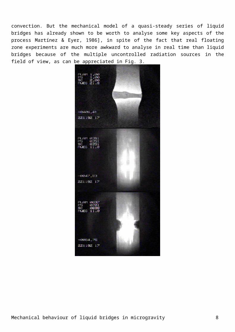
power (less than a second between both images); the last one shows a small liquid gap (perhaps only superficial) before all the silicon solidifies.

THEORETICAL RESULTS IN THE MECHANICAL BEHAVIOUR OF LIQUID BRIDGESFor the theoretical analysis of the mechanics of liquid bridges, one usually takes the general Navier-Stokes equations, introduces some drastic assumptions (e.g. zero velocity for static shapes, sinusoidal motion for periodic vibrations), adds some well-defined loads (boundary conditions, as perfect anchorage of the interface to the edges of the discs, a precise residual acceleration, perfectly known liquid volume, etc., and runs the computer to find by symbolic computation a few analytical approximations, and by numerical computation a lot of particular numerical approximations that are collected in a graphical image showing the loci of results along selected parametric families.

Although the theoretical foundations of these studies are well known (Young-Laplace capillarity equation at the interface and Navier-Stokes equations in the bulk), because of their non-linear behaviour, the solutions are difficult to obtain, what, added to the great variety of boundary conditions of interest, makes the analysis too cumbersome (one must resort to a multiparametric bunch of numerical computations difficult to grasp).

Some reviews of the mathematical formulation for the statics and dynamics of liquid bridges, as well as some experimental results, can be found in [Alexander, 1997] (where the problem of the modelling of contact lines is also presented), [Meseguer, Slobozhanin & Perales, 1995] and [Martínez,, Haynes & Langbein, 1987], to name a few, but it seems appropriate here to summarise the general equations used to analyse liquid bridges, and not only from the mechanical point of view but within a wider perspective, in order to pinpoint where the main difficulties in the modelling lay, both on ground (e.g. non-linear effects due to the curvature of the interface) and on space (e.g. g-jitter).

The most general equations, with the main restriction of assuming incompressible fluids except for the buoyancy term (Boussinesq model), can be grouped in: Internal conservation equations (applicable to fluid particles inside the liquid bridge as well as to those in

the surrounding fluid):

-continuity: 22\* MERGEFORMAT ()

-momentum: 33\* MERGEFORMAT ()

-species: 44\* MERGEFORMAT ()

-energy: 55\* MERGEFORMAT ()where , is the kinematic viscosity, g is a constant gravity field (used to model ground conditions), is the thermal expansion coefficient (this is the Boussinesq term to model natural convection on Earth), and is a generic g-jitter term, i.e. a time and direction varying function that accounts for the acceleration of the reference frame (the foundations of test-rigs in a space platform


cannot be as rigid as on ground). Di is the diffusion coefficient for species i in the mixture, yi is the mass fraction of species i, cS is related to the thermo-diffusion coefficient (the Soret effect; the Dufour effect is not included in (3) being negligible in liquids far from the critical state), wi stands for a possible generation of species i in reactive processes, is the thermal diffusivity, is the standard enthalpy of formation of species i, cp is the specific thermal capacity, and e stands for a possible generation of energy per unit volume by any heat release process.

Interfacial compatibility equations , that, together with the conditions at the solids bounding the liquid bridge and the external fluid (where the usual assumption is of equilibrium between fluid and solid), constitute the boundary conditions for the internal equations. Let 0=F(r,,z,t)=r-F(,z,t)=r-R0-f(,z,t) be three usual forms of the equation describing the evolving 3D-surface in cylindrical coordinates; the first is a generic surface, the second an explicit form in the radial coordinate, and the third a radial explicit form of the departure of the surface relative to the cylinder r=R0. The unit normal vector is , and its curvature

. If []=outer-inner represents the jump in the value of a function across the interface, the boundary conditions read:

- continuity: , or , 66\* MERGEFORMAT ()

-momentum: , or 77\* MERGEFORMAT ()

-energy: 88\* MERGEFORMAT ()where is the mechanical stress tensor ( is the viscous stress tensor), is the unit tensor, is the unit vector in the radial direction, is the interface tension between the inner and outer fluids, k is the thermal conductivity and eF stands for a possible external thermal energy source per unit area at the interface (e.g. absorption of radiation in a mirror furnace). All -operators refer to the corresponding space variables (some are 3D and others 2D).

Initial conditions (quite easy to postulate in the analysis, but quite difficult to control in a real microgravity experiment).

Sometimes, for low viscous fluids and outside boundary layers, the assumption of irrotational flow is plausible, , what implies also a potential flow, , changing the continuity equation to 2=0, and reducing

the momentum equation to Bernoulli equation:


-in the two bulk phases: =constant along a streamline,99\* MERGEFORMAT()

-at the fluid interface: , 1010\* MERGEFORMAT ()

and , 1111\*MERGEFORMAT ()

greatly simplifying the analysis; e.g. for normal mode analysis in the axisymmetric case, one tries solutions of the form =0exp[i(kz-t)] and f=f0exp[i(kz-t)] in the above equations to find the relation between eigenfrequencies and eigenmodes, i.e. the dispersion relation, =(k).

Additionally, in the presence of electric fields, the absence of free charges in normal fluids means that the Laplace equation, 2=0, applies to the electrical potential in the bulk phases, without any interaction with the flow equations above, but an electrical pressure, pE, to be added to the capillary pressure above, appears at the interface, that depends on the distribution of the electrical potential, the permitivities of the fluids and the geometry of the interface, pE(,inner,outer,F(,z,t))

In order to give a more structured idea of the several available theoretical models and results, the instantaneous states of a liquid bridge can be classified in the two following types to be subsequently examined:

Statics: equilibrium states and stability limits Dynamics: steady states, periodic states (oscillations), transient states (breakages).

Statics

This is the simplest case, and if only constant mechanical forces are acting, shapes can be easily computed as explained above, as well as the limit of stability along some direction in parameter space. Perhaps the best single parameter to distinguish shapes among themselves is the radius at a quarter of the bridge span, at least for axisymmetric shapes, because although the radius at the middle of the bridge seems sounder, it is unsuitable in the case of natural or forced oscillations in the first eigenmode, what is of paramount importance because of the omnipresent g-jitter in space. The following parameters have been investigated analytically and numerically, and the main results obtained are presented.

Geometry . Nominal geometry consists of a cylindrical liquid bridge anchored to the edges of two equal circular, planar, coaxial discs of radius R0 a distance L apart. Additional geometries studied are non-equal discs, non-planar discs (not considered), or non-coaxial discs (eccentric). Taking the disc radius (or the mean value) as unit length, the non-dimensional parameters that appear are:

=L/(2R 0), the slenderness of the bridge. Most experiments on statics of liquid bridges are for of order 3. The bridge span is always the main characteristic of a bridge, and for unloaded cylindrical bridges, is the only non-dimensional parameter. The bridge is stable for <, the Plateau-Rayleigh limit and unstable for > (Rayleigh in 1900 deduced this limit). Experimentally, Plateau in 1873 found max,cyl=3.13 in a neutral buoyancy tank (named Plateau


tank in his memory), Mason in 1970 found max,cyl=3.140 in a Plateau tank with discs of 6 mm in diameter, and in microgravity, the maximum value found seems to be max,cyl=2.92 with a 35 mm in diameter liquid column aboard Spacelab-D1 in 1985.

V=V/(R02L), the ratio of actual liquid volume to the cylindrical one. For unloaded bridges

between equal coaxial discs, the stability region in the (V,)-diagram is shown in Fig. 4. Equilibrium shapes of liquid bridges can be axisymmetric or non-axisymmetric (the latter only for very small or very large volumes), but practical interest is on axisymmetric liquid bridges with a volume not far from that corresponding to the cylindrical shape, V=1, and thus a lot of effort has been devoted to the analysis in the case v=V-1<<1. To characterise the shape in a single parameter one may use the extreme radius, i.e. the radius at the centre plane between discs, where the bulge or neck appears, but it is better to use the radius at a quarter of the length, R¼, because this is also applicable to amphora-like deformations appearing with other loads. Thus, there is interest to have analytical or numerical expressions for R¼(V,) and for the limit-of-stability values R¼(Vmin,) and R¼(V,max). To characterise the stability limits one looks for Vmin() and max(V). A handy approximation in this respect may be the tangent at the point (,1) in Fig. 4:

1212\* MERGEFORMAT ()

Fig. 4. Stability diagram for unloaded liquid bridges of volume V between equal discs of radii R a distance L apart [Da Riva & Martínez, 1979]. Transitions to non-axisymmetric shapes may be quasi-static or dynamic [Slobozhanin, Alexander & Resnick, 1997].


KR1/R2, the ratio of disc diameters, smaller/larger. Now for unequal coaxial discs, a three-dimensional (V,,K)-space should be considered. Again, bridges can be axisymmetric or non-axisymmetric (but never cylindrical), and if the radius at one quarter is chosen to identify the shape, analytical or numerical expressions are needed for R¼(V,,K) and for the limit-of-stability values R¼min(Vmin,,K), R¼min(V,max,K) and R¼min(V,,Kmin). To characterise the stability limits one looks for Vmin(,K), max(V,K) and Kmin(,V). If a value of K is fixed, the stability diagram is similar to the one in Fig. 4 but with a smaller stability region [Martínez, 1983, Martínez & Perales, 1986, Slobozhanin, Gómez & Perales, 1995]. This parameter, K, is of importance in the application to crystal growth by the floating zone process, because there the radii at the ends of the molten zone change during the initial and final phase of the processing (see Fig. 3).

eRE/R0, the non-dimensional separation between the (parallel) axes of the two non-coaxial discs being at a distance of 2E. Now shapes are always non-axisymmetric. The stability region also shortens [Laverón & Perales, 1995]. At present, no application has been envisaged for this configuration.

Liquid properties . Nominal liquid properties are assumed similar to those of water in the following sense: densities of liquids used, like silicone-oils, are nearly that of water (mercury e.g. has not been used); surface tension of liquids used are typically a few tenths of that of water; viscosity of liquids used is the more variable parameter, ranging from a few tenths of that of water to several order of magnitude larger, what has a proportional impact on transient phenomena like breaking time. Other liquid properties like the Prandtl number, Pr=cp/k, and the capillary number, Ca=T(T-T0)/0 where T is the derivative of surface tension with temperature and 0 a reference value, do not appear in isothermal liquid bridge behaviour. The only non-dimensional number sometimes introduced is:

ratioouter/inner, the density ratio of outer to inner fluids, what is neglected for liquid bridges surrounded by a gas, or the ratio between the difference in densities and a mean value, what is neglected for liquid bridges surrounded by an isodense immiscible liquid, as in a Plateau tank.

Loads . The nominal microgravity load in theoretical analyses is assumed to be nil (against what experimenters have painfully learnt in actual flights with the uncontrollable g-jitter). Usually the following static loads are additionally considered in the analysis:

BoAgR2/, the axial Bond number, the ratio of a residual axial body force (due to a constant axial acceleration) to surface tension forces (be aware of our using length R instead of L to define the axial Bond number, contrary to other authors). The combined effect of an axial Bond number and disc inequality for different volumes and slenderness of liquid bridges has been much studied [Slobozhanin, Gómez & Perales, 1995] because, each one of them reduces the stable region, but because the two effects are non-symmetric with respect to the middle plane between the discs, when both effects are in opposition they can compensate to a certain extent (this happens when axial gravity is directed towards the smaller disc).

BoLgR2/, the lateral Bond number, the ratio of a residual lateral body force to surface tension forces. This load always yields non-axisymmetric deformations.


We2R3/, the Weber number, the ratio of a centrifugal to surface tension forces. Since the pioneering analysis on the centrifugal stability of a cylindrical liquid bridge [Martínez, 1978], many contributions have extended the work: the effect of eccentric rotation was studied both theoretical [Perales, Sanz & Rivas, 1990] and experimentally, and the effect of an axial Bond number on the maximum stable Weber number Wemax(,Bo) has been recently computed [Slobozhanin & Alexander, 1997 & 1998].

In summary, leaving apart electric and magnetic effects, the hydrostatics of liquid bridges ( =0 above) is completely defined by the set of parameters , V, K, e, BoA, BoL and We, that is, the equilibrium shapes are described by the Young-Laplace equation, which in dimensionless variables reads [Meseguer et al., 1995]:

1313\* MERGEFORMAT ()

and the boundary conditions:

, 1414\* MERGEFORMAT ()

, 1515\* MERGEFORMAT ()

. 1616\* MERGEFORMAT ()

To write down the above expressions all lengths have been made dimensionless with R0=(R1+R2)/2; F=F(z,) stands for the shape of the interface, M for its curvature (a non-linear function of the arguments shown), P is a constant related to the difference between the outer pressure and the inner pressure at the origin of z (midway between discs) and made dimensionless with /R0. The subscripts z and indicate partial derivatives with respect to the axial and azimuthal coordinates.

A handy general approximation for the lower stability limit may be given for small values of the distorting parameters relative to the cylindrical shape (with h=(1-K)/(1+K)<<1) [Laverón & Perales, 1995]:

1717\*MERGEFORMAT ()

where is the azimuthal angle between the plane of the non-coaxial axes of the discs and the direction of the lateral acceleration. Observe the possible compensation amongst antisymmetric effects already explained.

Although in real microgravity experiments there is a time-varying load (g-jitter) seldom considered in theoretical analysis, the later may give clues such as whether the liquid bridge is more sensitive to axial or lateral accelerations of the same magnitude, both concerning shape deformation and the stability criteria, as can be deduced from Meseguer et al. 1995a and is presented in Fig. 5.


Fig. 5. Comparison of the sensitivity of an initially-cylindrical liquid bridge of slenderness L/(2R) to axial and lateral static accelerations measured by their respectives Bond numbers BoA and BoL [after Meseguer et al, 1995]; a) Maximum stable Bond number, b) deformation of the shape per unit Bond number (gain). An axial load causes an amphora-like radial axisymmetric deformation, and a lateral load causes a C-mode deformation of the line of centres (the initial axis of symmetry).

Dynamics

In this case, time is the most important variable. Besides all the transient problems encountered during the formation of a long liquid column (emerging capillary flows, detachment, spreading, anchoring, filling liquid, separating the discs, removing liquid, etc), some transient problems with already established cylindrical liquid columns are of interest. Particular attention has been paid to the evolution during the breakage of the column beyond the stability limit [Meseguer, 1983] and to the cylindrical liquid injection (injection and separation to keep a cylindrical volume) [Martínez & Sanz, 1985]. Transient problems require such a strict control of the initial conditions, and demand such a comprehensive diagnosis (with variables changing their ranges and relative importance through the evolution) that no attempt to have detailed quantitative measurements has yet been exercised in a microgravity platform.

A lot of work has been devoted to periodic or steady problems. Here, the time variable can be taken out of the problem because it does not appear (steady states) or because it enters as a separate harmonic term (periodic states) that modulates in a simple manner the spatial response (the period is well defined). Typical problems in this field are the periodic oscillations of the column when one (or both) of the end supports is forced to oscillate axially or laterally, the steady state reached when one of the discs is forced to rotate at a constant rate (or both, at equal or different speeds), the flow induced inside the liquid bridge by a uniform shear outer flow, etc. In these cases, besides the outer shape of the bridge, the relative motion inside the fluids is also of great interest. Steady state theories are less developed, and a lot remains to be done (e.g. how is the flow structure in a counter-rotating liquid column).

Other degrees of freedom appear on dynamical problems, as the transport coefficients: viscosities of working liquid and outer fluid, and the ratio of viscous to capillary forces. The new dimensionless parameters are:


ratioouter/inner, the viscosity ratio of outer to inner fluids, what is neglected for liquid bridges surrounded by a gas, but may be dominant for liquid bridges surrounded by an isodense immiscible liquid, as in a Plateau tank.

Oh , the Ohnesorge number, the ratio of viscous to capillary forces, a kind of inverse Reynolds number.

Besides, the forcing parameters introduce other non-dimensional parameters like:

(2R3/)1/2, the non-dimensional forcing frequency, also interpreted as a kind of Weber number that compares inertia forces to capillary forces.

The techniques used to simplify the analysis of the dynamics of liquid bridges have been: One-dimensional models [Perales & Meseguer, 1992], borrowed from jet theory, and only

applicable to the most interesting case of long liquid bridges. Axisymmetric potential models [Sanz, 1985]. Linearised or weakly non-linear models around a basic cylindrical shape [Nicolas & Vega, 1996]. Averaged models, where the first order vibrations are averaged to analyse the secondary flow

(streaming) [Nicolas, Rivas & Vega, 1997, Nicolas, Rivas & Vega, 1998].

The resonant frequencies have been calculated in the past by using three-dimensional models (which allow a precise consideration of inertial terms) in the inviscid case and considering a small viscosity for cylindrical liquid bridges. If the volume is not cylindrical or the discs are not of equal diameter and concentrical, the analytical solutions based on three-dimensional models are no longer possible and numerical schemes based in one-dimensional models are to be used. As an example of the many results on the eigenfrequencies of cylindrical liquid columns, Fig. 6 shows the first eigenfrequencies of a cylindrical volume liquid bridge [Sanz, 1985]. The effect of the viscosity has also been studied, see e.g. [Nicolás & Vega, 1996].

Fig. 6. Non-dimensional eigenfrequencies (2R3/)1/2, vs. slenderness L/(2R), for the inviscid axisymmetric motion of cylindrical liquid bridges. Results from a three-dimensional model.


Concerning the forced response of a liquid bridge when one (or both) of the supporting discs are oscillated, or when the gravity field changes with time, mainly one-dimensional models have been used up to now [Perales & Meseguer, 1992]. These models, although easily allow the consideration of the viscous effects, introduce uncertainties in the consideration of inertial effects. In effect, they are based in averaging the velocity field and assuming a given radial variation of it. This hypotheses can be justified as far as the bridge is slender enough but precludes the application of the model for short liquid bridges or large excitation frequencies. As an example of the response of a cylindrical liquid column to forced oscillations imposed to the liquid column by vibrating the supporting discs (with particular attention to the in phase or in counter-phase cases), Fig. 7 presents some theoretical results using a linear three-dimensional model in which viscosity effects are not considered.

Fig. 7. Transfer function (maximum interface deformation of the liquid bridge divided by the amplitude of the forcing perturbation, F=R/Zdisc), vs. non-dimensional forcing frequency (2R3/)1/2, for an inviscid cylindrical liquid bridge of slenderness =3, for the case of antisymmetric excitation (a, both discs in counterphase, deformation even for =0), and symmetric excitation (b, both discs in phase). If a sinusoidal variation of gravity level were considered, the transfer function could be deduced from plot b by simply plotting instead the ordinate divided by 2. Results from a three-dimensional model (bold lines) and from a Cosserat one-dimensional model (dashed).

EXPERIMENTAL RESULTS IN THE MECHANICAL BEHAVIOUR OF LIQUID BRIDGES

The need and objectives of experiments

All theories encompass some hypotheses and simplifications that must be checked if they are applicable or not, and in practice, unthought-of effects always appear. Thus, the general purpose of experiments with liquid bridges (applicable to many other problems) may be stated as follows: 1. To check that the response of the system to the applied stimuli is as predicted by theory. To this purpose,

clear-cut check points are proposed for measurement (e.g. minimum volume of liquid for a stable bridge), with well controlled applied stimuli (precision control of disc separation, rotation and vibration) and little sensitivity to uncontrolled forces (e.g. working temperature, g-jitter, liquid contamination). Thus, a set of non-dimensional parameters (,V,h,e,BoA,BoL,We) is applied and the actual shape is recorded (the actual experiment); later, from those shapes, by digitisation and convolution aided by previous theory, the best matching set of experimental values is obtained (data analysis); finally, by comparing both sets of parameters, and, after the uncertainties due to experimental error have been accounted for, one tries to explain the differences found (conclusions).


2. To check if the assumed hypothesis hold. When the response of the system is not as expected (what happens most of the times at the beginnings), the consistency of the theoretical development must be reviewed, and thence the applicability of the hypothesis introduced to simplify the analysis or to model the system (e.g. is evaporation of no effect?).

3. To see if new phenomena appear, and to quantify them. For instance, if a theory to account for the effect of the residual acceleration is available, and in this case it is, the experiment may allow to estimate the actual value.

Large liquid bridges can only be established under microgravity; on ground, quiescent fluid interfaces are always flat except at the corners and other small-scale regions (of a few millimetres). The shortest time to create a large liquid column (35 mm in diameter and 100 mm long) is nearly one minute, what precludes experimentation in short-time microgravity platforms as drop towers and parabolic flights with airplanes. The 6 minutes of microgravity time provided by the TEXUS sounding rocket has already been proved adequate for single experiments in the mechanical behaviour of the liquid, but are too short for more detailed redundant and multiparametric experiments.

During experiment execution in Spacelab-D1 the ambient mechanical noise (so called g-jitter) forced the liquid to be in a permanent state of motion, although fortunately of small amplitude. Instead of just concluding that Spacelab was found to be a noisy environment not suitable to delicate experiments with liquid bridges at equilibrium, a deep analysis of the consequences has been performed, trying to extract the maximum of information from the available (rare, unique and costly) data.

The aim of mechanical experiments with liquid bridges under microgravity has been mainly twofold: a) Measuring the static deformation of the outer shape near their stability limit, caused by some controlled

mechanical disturbances (change of geometry, change of volume, rotation and vibration), or by a residual acceleration. An experiment on equilibrium shapes consists of procuring a well-defined configuration (geometry and liquid) and constant stimuli, to measure the shape of the bridge and changing the parameters quasi-steadily to find the stability limits.

b) Measuring the dynamic response (analysing also the outer shape deformation) when applying a controlled vibration of one or the two solid supports, or by natural g-jitter due to the spacecraft. An experiment on vibration consists of procuring a well-defined configuration (geometry and liquid), initiating a periodic stimuli, and waiting to the periodic response to measure the oscillation in shape of the bridge, changing the parameters quasi-steadily to find the eigenfrequencies.

Past experiments

Experiments with liquid bridges were initiated on ground by Plateau in the XIX century, using the isodense-bath technique he discovered. Little work on liquid bridges followed, both experimental or theoretical, until the space era in the late 1960s, where the need to know better about capillary systems, and the opportunity to experiment with them in a much better environment than on ground, arose.


Experiments in microgravity conditions have the main advantage that hydrostatic forces and buoyancy forces nearly disappear and one may work with large fluid samples. On the other hand, the loss of the perfectly defined and constant gravity field on ground has its own disadvantages: the constancy is also lost, and the residual microgravity field is unknown, uncontrolled, and varying with time, direction and intensity, what is a severe handicap for any kind of experiment.

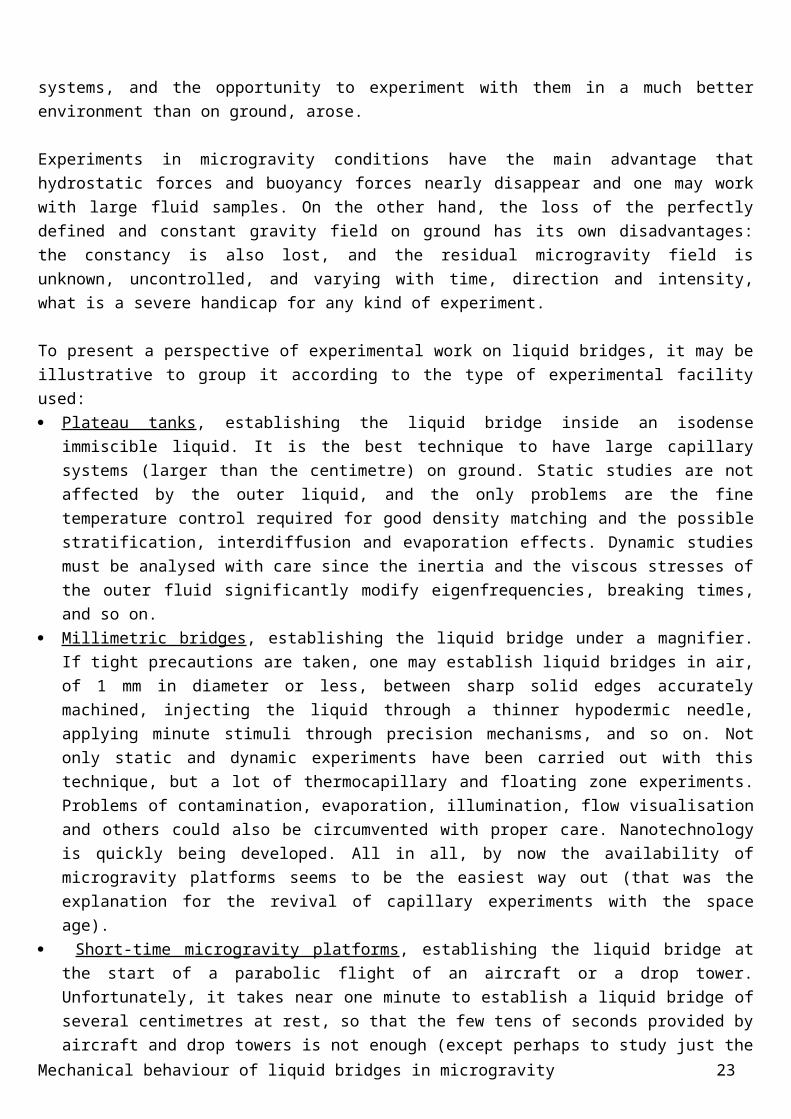
To present a perspective of experimental work on liquid bridges, it may be illustrative to group it according to the type of experimental facility used: Plateau tanks , establishing the liquid bridge inside an isodense immiscible liquid. It is the best technique to

have large capillary systems (larger than the centimetre) on ground. Static studies are not affected by the outer liquid, and the only problems are the fine temperature control required for good density matching and the possible stratification, interdiffusion and evaporation effects. Dynamic studies must be analysed with care since the inertia and the viscous stresses of the outer fluid significantly modify eigenfrequencies, breaking times, and so on.

Millimetric bridges , establishing the liquid bridge under a magnifier. If tight precautions are taken, one may establish liquid bridges in air, of 1 mm in diameter or less, between sharp solid edges accurately machined, injecting the liquid through a thinner hypodermic needle, applying minute stimuli through precision mechanisms, and so on. Not only static and dynamic experiments have been carried out with this technique, but a lot of thermocapillary and floating zone experiments. Problems of contamination, evaporation, illumination, flow visualisation and others could also be circumvented with proper care. Nanotechnology is quickly being developed. All in all, by now the availability of microgravity platforms seems to be the easiest way out (that was the explanation for the revival of capillary experiments with the space age).

Short-time microgravity platforms , establishing the liquid bridge at the start of a parabolic flight of an aircraft or a drop tower. Unfortunately, it takes near one minute to establish a liquid bridge of several centimetres at rest, so that the few tens of seconds provided by aircraft and drop towers is not enough (except perhaps to study just the g-jump in a partially balanced Plateau tank). In spite of this handicap, the many experiments carried out by Padday aboard parabolic flights should be mentioned, particularly those related to the effect of viscosity on breakage, where it is shown that a low viscosity liquid bridge yields a satellite drop when breaking, but a very high viscous one yields an evanescent liquid thread (Padday et al, 1997).

Sounding rockets of 6 to 15 minutes of microgravity. This is a most valuable platform to perform single mechanical experiments with liquid bridges. Very good results have been obtained, e.g. concerning the deformation and breakage of a cylindrical liquid column when subjected to eccentric centrifugation [Sanz, Perales & Rivas, 1992], and the controlled forcing of a quasi-steady axial load [Martínez, Perales & Meseguer, 1996]. Several versions of ESA’s Liquid Column Cell, where a cylindrical liquid bridge is established in a single stroke by separating a hollow disc from the other (Fig. 8) have been flown. However, the handicap of being a one-shot trial without repetitivity, renders orbiting platforms more convenient.

Orbiting platforms , mainly the Spacelab, where a series of trials with the same liquid bridge in the same set-up, formation of several new bridges and controlled breakages, were performed using different versions of ESA’s Fluid Physics Module.


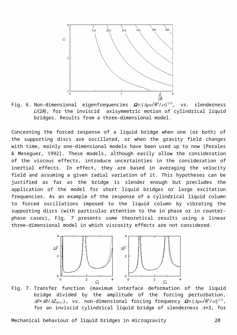
Fig. 8. Experiment on a quasi-static calibrated microgravity acceleration (100 1 g), well above the uncontrolled g-jitter of the platform, of a liquid bridge on Texus-33 [Martínez, Perales & Meseguer, 1996]. A silicone oil 10-times more viscous than water was used. First the liquid bridge is established between discs of 30 mm in diameter, initially touching (first frame), then displacing one up to 85 mm (second frame), and then forcing a gentle oscillation of the whole experimental cell up and down (100 mm peak-to-peak with a 45 s period) as evidenced by the parallel solid bar seen on


the field-of-view but that was kept fixed to the rocket and not to the cell (frames 3 and 4). The final two frames show the liquid bridge breakage at the uncontrolled reentry of the capsule (observe how different it is respect to Fig. 2 also taken in another Texus flight).

Most of the reported results refer to quasi-static experiments. Dynamics is harder to analyse. Notwithstanding the fact that the dimension of the problem has grown (still confining oneself to axisymmetric motions), a major experimental handicap appears concerning the diagnosis of the motion inside the liquid column, what is very difficult because its curved interface (particularly if it is not nearly-cylindrical) renders the optical diagnosis cumbersome. Small tracer particles added to the liquid are normally used for qualitative visualisation (as was done in these experiments) making them visible with a meridian light sheet, but quantitative analysis has always somehow resisted.

In the whole, the achievements from so many experiments on the mechanics of liquid bridges might look meagre, but it must be agreed that liquid management with free boundaries under microgravity is not an easy task. For instance, the sophisticated liquid-injection system developed for the Fluid Physics Module (FPM) in 1977, was of little use in the first Spacelab flight in 1983, due to infancy operating problems during real microgravity conditions. On the one hand, the 0.5 mm protrusion on the solid supports proved to be insufficient to anchor the liquid edge (perhaps due to precursor film spreading); on the other hand the FPM was cumbersome to operate by the astronauts and, after a few initial trials, air bubbles were ingested while trying to recover liquid from spillages, and the liquid supply became useless. For the second FPM flight (1985) an add-on manually-driven liquid injection system was provided, but then it proved unrealistic to expect that an astronaut stressed to the limit (working in a multitask, multi-surveyed, round-the-clock, heavy demanding environment) would waste precious time of pioneering experiments just reading a counter and writing sets of numbers in a piece of paper. In spite of great progress and some quantitative results, Fig. 9 gives a good idea of the difficulties faced during past experiments in microgravity.


Fig. 9. Some lessons learnt from past liquid bridge experiments [Martínez, Perales & Meseguer, 1995]. A) Difficulties in liquid bridge visualisation on experiment Spacelab-D1-FLIZ due to usage of a mirror box. B) Presence of an air bubble inside a good cylindrical liquid column in experiment Spacelab-D2-STACO run 2. C) An instant after an intentional breakage of a liquid bridge in Spacelab-D2-STACO run 2, where an imminent overflow of the big drop beyond the sharp edge of the solid disc


can be seen, contrary to several other intentional breakages perfectly recovered during Spacelab-D1-FLIZ.

PROSPECTIVE Capillary experiments were difficult to perform on ground before the advent of microgravity platforms and this may explain the blooming up of trials in the last 30 years. The second wave of this blossoming could be expected to come with the availability of plenty of microgravity time in the International Space Station.

Easily accessible data bases as ESA MGDB (http://www.esrin.esa.it/htdocs/mgdb/) and NASA MICREX (http://mgravity.itsc.uah.edu/microgravity/micrex/) have been major efforts to compile exhaustive references to past microgravity experiments, including not only the flight experiment details but the publications directly related to the preparation and those of postflight analysis. They allow to find entries by subject matter, keywords, authors, date, mission, facility, etc. In spite of the handicap of the old documentation technology used (scarce, if any, equations, drawings, graphics, images, and so on), they help very much to disseminate very costly findings and must be fostered in the future.

The importance of liquid bridge research and the microgravity relevance have been justified above, and the fact that it was pioneering and has 20 years of experience does not mean that the subject has been harvested and is ended. If one considers that there is still great controversy on how to quantify the microgravity environment it is clear that we are at the beginnings. To support this with a last example, we present in Fig. 10 a still unexplained behaviour of a liquid bridge in microgravity.


Fig. 10. Unexplained breakage of a liquid bridge in Spacelab-D2-STACO run 3 [Martínez, Perales & Meseguer, 1995]. In this run, a similar cylindrical liquid column as in Fig. 1 was established a week later, but this time the astronaut reported much observed ‘g-jitter’ in the liquid (the recordings of the solid-state accelerometers didn’t explained that) and, notwithstanding the fact that everything was left idle to avoid perturbations, in a few seconds (see time-tagged frames) a neck developed


(first frame), then it changed to the other side of the liquid bridge (middle frame) and finally broke down (last frame).

Future experimental opportunities

Several major infrastructures to support experiments in the International Space Station are being developed, particularly the Fluid Science Laboratory for what concerns liquid bridge research, but the details of the fluid volume configuration and stimuli have been left open. In this scenario, an FSL Experiment Container to study liquid bridges should be developed, presumably to serve a variety of objectives, as it was in the past. To this aim, operations in a fluid science laboratory in space must be considered from the beginning, and, since the design cannot be tailored to a single trial, a trade off study would be required on :

what kind of liquid bridges experiments under microgravity may be expected what kind of equipment is needed in support of these experiments how operations are envisaged to achieve those goals with these means.

This philosophy of common multi-user facilities is the only affordable approach to experiments in space, but posses some constraints on candidate experiments, thence, it is expected that in the future there will be more off-the shelf equipment and processes, with well-advertised characteristics, and the experimenter will devote more time to assemble this flow of information in the most appropriate way, instead of the old style of designing unique pieces of equipment, unique pieces of software and unique procedures. The several hours of past experience on liquid bridges research aboard Spacelab and other minor microgravity platforms have taught many lessons to both the investigators and the operations teams, and this must not be forgotten.

First, and above all, the major handicap that fluid science investigators have suffered in the past is the scarcity of microgravity time. Sporadic opportunities can only give as a return sporadic scientific achievements. The availability of microgravity time at a reduced cost is a requirement for the build up of a mastery in fluid science in space. Although it is a broader policy issue and not a scientific one, it must be realised that microgravity experiments cannot be charged with the costs of space infrastructure and general operations, and only with direct additional costs as energy, crewtime, fluid science equipment, fluid science operations, and so on.

Last but not least, another ingredient genuine to microgravity research, but that has shown particularly clear with liquid bridge experiments is the proper characterisation of g-jitter.

REFERENCES

1. Alexander, J.I.D., 1997, “Drops, jets and bubbles”, in “Free surface flows”, Kuhlmann, H.C. & Rath, H.J. (eds.), Springer-Verlag.

2. Concus, P. & Finn, R., 1998, “Discontinuous behaviour of liquids between parallel and tilted plates”, Phys. Fluids vol 10, pp.39-43.

3. Da Riva, I. & Martínez, I., 1979, “Floating Zone Stability”, ESA SP-142, pp. 67-73.


4. Laverón, A. & Perales, J.M., 1995, “Equilibrium shapes of non-axisymmetric liquid bridges of arbitrary volume in gravitational fields and their potential energy”, Phys. Fluids, vol. 7, pp. 1204-1213.

5. Martínez, I. & Cröll, A., 1992, “Liquid bridges and floating zones”, ESA SP-333, París, pp. 135-142.

6. Martínez, I. & Eyer, A., 1986, “Liquid bridge analysis of silicon crystal growth experiments under microgravity”, J. Crystal Growth 75, pp. 535-544.

7. Martínez, I. & Perales, J., 1986, “Liquid Bridge Stability Data”, J. Crystal Growth, vol. 78, pp. 369- 378.

8. Martínez, I. & Sanz, A., 1985, “Long liquid bridges aboard sounding rockets”, ESA Journal, 9, pp 323-328.

9. Martínez, I., 1978, “Floating Zone. Equilibrium Shapes and Stability Criteria”, Space Research XVIII, pp. 519-522.

10. Martínez, I., 1983, “Stability of Axisymmetric Liquid Bridges”, in “Materials Sciences under Microgravity”, ESA SP-191, pp. 267-273.

11. Martínez, I., Haynes, J.M. & Langbein, D., 1987, “Fluid Statics and Capillarity”, in “Fluid Sciences and Materials Sciences in Space”, H.U. Walter (ed.), Springer-Verlag.

12. Martínez, I., Perales, J.M. & Meseguer, J. 1996, “Response of a Liquid Bridge to an Acceleration Varying Sinusoidally with Time”, Lecture Notes in Physics, vol.464, pp. 271-282.

13. Martínez, I., Perales, J.M., Meseguer, J. 1995, Stability of long liquid columns (SL-D2- FPM-STACO), in Scientific Results of the German Spacelab Mission D-2, Ed. Sahm, P.R., Keller, M.H., Schiewe, B, WPF, pp. 220-231.

14. Martínez, I., Sanz, A., Perales, J.M. & Meseguer, J., 1988, “Freezing of a long liquid column on the Texus-18 sounding-rocket flight”. ESA Journal 12, pp. 483-489.

15. Meseguer, J., 1983, “The breaking of axisymmetric slender liquid bridges.”, J. Fluid Mechanics 130, pp. 123-152.

16. Meseguer, J., Bezdenejnykh, N.A., Perales, J.M. & Rodríguez de Francisco, P., 1995, Theoretical and Experimental Analysis of Stability Limits of Non-Axisymmetric Liquid Bridges, Microgravity Science and Technology, vol. 8, pp.2-9.

17. Meseguer, J., Slobozhanin, L.A., & Perales, J.M., 1995, “A review on the stability of liquid bridges”, Advances-in-Space-Research. vol.16, pp.5-14.

18. Nicolas, J.A. & Vega. J.M., 1996, “Weakly nonlinear oscillations of nearly inviscid axisymmetric liquid bridges”, Journal of Fluid Mechanics, 328, pp.95-128.

19. Nicolas, J.A., Rivas, D. & Vega. J.M., 1997, The interaction of thermocapillary convection and low-frequency vibration in nearly-inviscid liquid bridges, Zeitschrift-fur-Angewandte-Mathematik-und-Physik, 48, pp.389-423.

20. Nicolas, J.A., Rivas, D. & Vega. J.M., 1998, “On the steady streaming flow due to high-frequency vibration in nearly inviscid liquid bridges”, Journal of Fluid Mechanics, 354, pp.147-74.

21. Padday, J.F., Petre, G., Rusu, C.G. Gamero, J. Wozniak, G., 1997, "The shape, stability and breakage of pendant liquid bridges", Journal of Fluid Mechanics 352, p.177-204.

22. Perales, J.M. & Meseguer, J., 1992, Theoretical and Experimental Study of the Vibration of Axisymmetric Viscous Liquid Bridges, Physics of Fluids A, vol. 4, pp. 1110-1130.


23. Perales, J.M., Sanz, A. & Rivas, D., 1990, “Eccentric Rotation of a Liquid Bridge”, Appl. Microgravity Tech., Vol. 2, pp. 193-197.

24. Sanz, A., 1985, “The influence of the outer bath in the dynamics of axisymmetric liquid bridges”, Journal of Fluid Mechanics, 156, pp. 101-140.

25. Sanz, A., Perales, J.M. & Rivas, D., 1992, “Rotational Instability of a Long Liquid Column”, in Final Reports of Sounding Rocket Experiments in Fluid Science and Materials Sciences ESA SP-1132 (Vol. 2), pp 8-21.

26. Slobozhanin, L.A. & Alexander, J.I.D.,1998, “Combined effect of disc inequality and axial gravity on axisymmetric liquid bridge stability”, Phys. Fluids, vol. 10, pp. 2473-2488.

27. Slobozhanin, L.A., Alexander, J.I.D. & Resnick, A.H., 1997, “Bifurcation of the equilibrium states of a weightless liquid bridge”, Phys. Fluids, vol. 9, pp. 1893-1905.

28. Slobozhanin, L.A., Alexander, J.I.D.,1997, “Stability of an isorotating liquid bridge in an axial gravity field”, Phys. Fluids, vol. 9, pp. 1882-1892.

29. Slobozhanin, L.A., Gómez, M. & Perales, J.M., 1995, Stability of Liquid Bridges between Unequal Disks under Zero-Gravity Conditions, Microgravity Science and Technology, vol. 8, pp.23-34.


physics of fluids in microgravity - upmwebserver.dmt.upm.es/~isidoro/lc1/c2/chapter2.docx · web...

Documents