PID Controller tuning and implementation aspects for building thermal control

KAFETZIS G. *, PATELIS P. *, TRIPOLITAKIS E.J. *, STAVRAKAKIS G.S. *,

KOLOKOTSA D. **, KALAITZAKIS K. ** Department of Electronic & Computer Engineering

Technical University of Crete Technical University of Crete, Kounoupidiana Campus, 73100, Chania, Crete

Greece ** Department of Natural Resources and Environment Laboratory of Renewable Energy

Resources Engineering Technological Educational Institute of Crete

3, Romanou Str, 73100, Chania, Crete Greece

http://www.elci.tuc.gr

Abstract: - The control of the indoor environmental parameters of buildings is an open problem with many practical difficulties which stem from the non-linear, multivariable nature of the building models. This paper presents the tuning process of a conventional PID controller for the thermal comfort control application, in buildings utilizing fieldbus systems. The PID controller has been chosen taking into account its widespread deployment and its attractive features like low computational cost and simplicity of implementation. On the contrary, there is no standard methodology for the extraction of its parameters. Therefore, empirical methods should be utilized along with trial and error techniques on the target application. The design procedure is illustrated and there is special focus regarding the practical aspects of the implementation on a laboratory installation. Finally, the results of the monitored and computed variables of the experimental procedure are presented along with relevant conclusions and discussion.

Key-Words: - PID controller tuning, process reaction curve method, thermal controller

1. Introduction One of the key design goals for building energy management systems (BEMS) is the reduction and minimization of the energy consumption. Moreover, along with the power saving goals, the indoor environmental parameters should be adjusted properly in order to ensure comfort conditions. Therefore, a control algorithm is necessary to provide a balance between comfort and low energy consumption.

Despite the scientific progress on the areas of building energy management systems and building networking applications, the design of an optimal control algorithm presents increased difficulty. This is due to the nonlinear characteristics of the building model. Moreover, it is difficult to efficiently use a set of linear state-space equations to describe this family of systems, as the existing ones present poor performance and lack generalization.

Several approaches have been proposed in order to overcome the nonlinearity of the building’s model. These include classic control approaches and intelligent system applications. Qu and Zaheeruddin

[1] proposed the transformation of H∞ loop-shaping tuning rules, to discrete-time tuning rules, in order to implement an adaptive PI controller for HVAC (Heating Ventilation and Air Conditioning Systems). Wang, Lee, Fung, Bi and Zhang [2] suggested a PID controller that presents high performance for a range of linear self-regulating processes, along with laboratory experimental results. Regarding intelligent control, Tripolitakis, Kolokotsa et al [3] suggested a Fuzzy PD controller for thermal comfort in buildings and Moshiri and Rashidi [4] proposed an adaptive self-tuning fuzzy PID controller for the control of nonlinear HVAC systems. Kolokotsa et al [5] introduced a genetic algorithms optimized fuzzy controller for the indoor environmental management of buildings. Huang and Lam [6], illustrated a genetic controller approach for the tuning of a conventional PID controller rules.

This paper describes the design, tuning and application of a digital PID controller for the adjustment of indoor conditions in the laboratory of Electric Circuits and Renewable Energy Sources at the Technical University of Crete. The PID

Proceedings of the 10th WSEAS International Conference on CIRCUITS, Vouliagmeni, Athens, Greece, July 10-12, 2006 (pp308-313)

controller is chosen due to its simplicity, low computational overhead and exceptional behaviour to a wide range of applications. The controller developed in this work, is implemented on a personal computer which communicated with the sensors and actuators using the European Installation Bus (EIB) infrastructure. The system inputs are received from a set of sensors which monitor the indoor and outdoor conditions. Such sensors are indoor and outdoor temperature, relative humidity, mean radiant temperature (MRT) and air speed. The output of the system controls two air-conditioning units of 36,000 btu each, used for both heating and cooling. The design objective is to adjust the indoor temperature to a desired set value, on the presence of external disturbances. Moreover, the resulting system should be able to compensate for the sensor inaccuracies, present fast convergence to the set point, minimum oscillation amplitude and minimum overshoot or undershoot.

Section 2 presents a brief introduction to the classic PID controller. Section 3 deals with the description of the Ziegler–Nichols methodology for the controller’s parameters tuning. On section 4, the tuning process along with the experimental results of the laboratory application of the controller, are presented. Finally, on the fifth section there is a short discussion about the contribution of this work.

2. Conventional PID Controller The conventional PID controller is the most popular controller in industry. Its wide deployment is justified due to its effectiveness along with simplicity of design and implementation. Despite its advantages, the design of such a controller is not described by a general methodology and focuses on empirical methods.

2.1 Analysis of the controller The PID controller consists of three parts: the Proportional gain (P), the integral gain (I) and the differential gain (D). Their general transfer function is given by:

)(sGc = + pKs

Ki + or dsKs

KsKsK ipd ++2

(1)

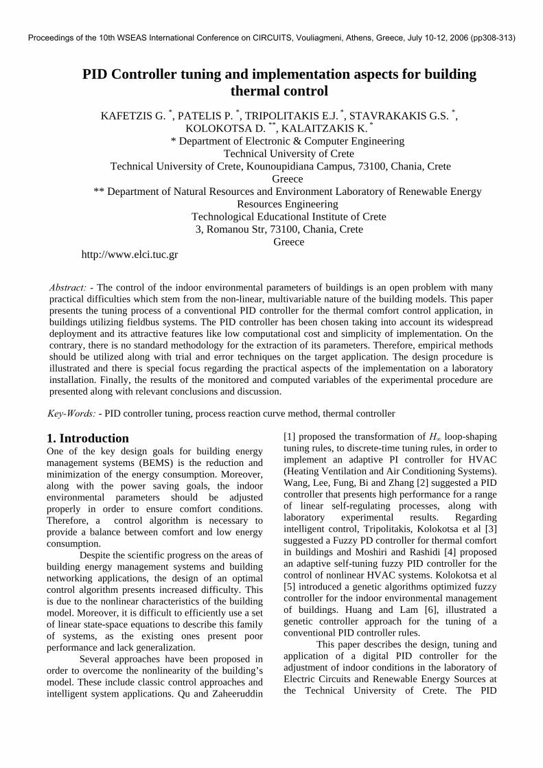
where the gains , and are the gains for proportional, integral and derivative part respectively. The general block diagram of a plant with a PID controller attached to it, is given on the following figure:

pK iK dK

Fig. 1, Block diagram of plant with a PID controller

An equivalent transfer function is given below:

⎥⎦⎤

⎢⎣⎡ ++==

sTsTK

sEsUsG i

dcc 1)()()( (2)

where = iTi

p

KK

is the integral constant, = dTp

d

KK

is the derivative constant and . The above transfer function can be transformed on the continuous-time domain giving the following equation:

cK pK≈

)( +)(1)()(0

⎥⎦

⎤⎢⎣

⎡+= ∫ dt

tdeTdeT

teKtu d

t

ic ττ (3)

If the sampling time has low value this equation can be transformed to a discrete-time differential equation. The differential term (D) is replaced by a first order expression of difference and the integral term (I) by a sum giving the equation on the discrete-time domain:

oT

⎥⎦

⎤⎢⎣

⎡−−++= ∑

−

=

1

))1()(()()()(k

oi o

d

i

oc keke

TTie

TTteKtu (4)

2.2 Characteristics of the PID controller 2.2.1 P controller The P part gain, is proportional to the input error value. It offers limited performance as it is unable to eliminate the steady state error. It is common to use the expression, Proportional Band (PB), to describe the action of the proportional gain. The

equivalent equation is given by: PB[%] = pK

100%

(5). 2.2.2 I controller The output of the integral part is proportional to the calculated sum of errors and demonstrates a way of slow reaction control. Moreover, it manages to eliminate the steady state error by generating respective actuation outputs and at the same time works against the oscillatory behaviour of the plant.

Proceedings of the 10th WSEAS International Conference on CIRCUITS, Vouliagmeni, Athens, Greece, July 10-12, 2006 (pp308-313)

2.2.3 D controller The derivative part gain is proportional to the rate of change of the control error. It leads to fast response stable systems at the cost of steady state error introduction and oscillatory behaviour.

3. PID Parameters Extraction The PID controller design objective is to determine a set of gains (or gains along with time constants) ( , , ) or ( , , ), pK iK dK cK dT iT in order to fulfill the performance requirements. These gains are to be calculated in such a way that the transient response, tolerance to disturbances and steady error specifications are met. In practice, it is not possible to achieve all of these requirements. Many researchers have tried to overcome these difficulties and obtain a global design method of PID controllers. As a result many methods for tuning single-loop and multi-loop PID controllers have been proposed. Some of these are: Ziegler-Nichols, Cohen and Coon, Ho-Hang-Cao and Internal model control. In this paper Ziegler-Nichols method is reviewed and used to calculate the PID controller’s parameters. 3.1 Ziegler-Nichols method In 1943 Ziegler and Nichols [7] proposed a method known as process reaction curve method. In this method, the open loop unit step response of the plant (the controller is disconnected from the system) is measured and approximated by small straight lines usually given a form as shown in figure 2.

Fig. 2, Plant unit step response

The tangent, in the point of the curve where the first derivative receives its maximum value is drawn (point of inflection). The dτ , T and K parameters are calculated below: Delay time 01 ttd −=τ (6) response time (7) 12 ttT −=

and gain0

0

uuyyK

−−

=∞

∞ (8)

The rules of Ziegler- Nichols method for the extraction of PID parameters are as shown in Table 1.

Parameters Controller

cK iT dT P

dKTτ

PI

dKTτ9.0

3.0dτ

PID

dKTτ2.1

dτ2 0.5 dτ

Table 1 – Controllers’ Parameters by Ziegler-Nichols method

It has to be noted that a major disadvantage of the Ziegler-Nichols method, is the undesired effect of oscillatory behaviour on a set of systems.

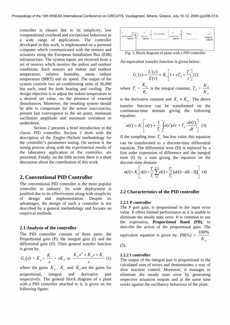
4. Experimental Procedure 4.1 General The PID controller used, is applied for the control of laboratory’s temperature and it has the basic characteristics of PID controllers, as they were given in the section 2. Figure 3 shows the block diagram of PID controller and its transfer function is given by eq. (4)

Fig. 3, PID block diagram

The inputs of the controller are three: the current temperature error, the sum of all past temperature errors and the temperature error difference, . The error is defined as the difference of the set-point, which is the desirable achieved temperature, from the present measured temperature, = set point - measured temp. The set point was selected at 28 °C as it was considered to be a suitable temperature for the summer season. The sum of errors is defined as the sum of all past temperature errors plus the current error. The error difference is defined as the difference between the current error and the previous error,

)(kce

)(ke

)1()()( −−= kekekce .

Process Reaction Curve

Tangent

Proceedings of the 10th WSEAS International Conference on CIRCUITS, Vouliagmeni, Athens, Greece, July 10-12, 2006 (pp308-313)

4.2 Extraction of the PID parameters The Ziegler-Nichols method was used as described in section 2, for the extraction of the , and

parameters. At first, while the controller was disconnected from the system (open loop), a unit step input was applied by setting the two air conditions to operate constantly at full power for an amount of time sufficient for the system to reach a steady state. Moreover, no other sort of HVAC control was performed on the installation. The period in which the measurements were taken was, at the end of July 2005.

cK iT

dT

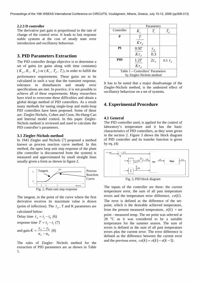
At the same time, temperature measurements were received every 2 minutes. The time of 2 minutes was chosen so as to yield dense measurements and provide good approximation of the temperature curve. The curve export procedure was applied for a number of days in order have a large set of measurements. As it can be deducted from figure 3, the laboratory temperature stabilizes slightly above 22 °C after 120 minutes. This happens because of the constant contribution of cooling to the laboratory space without any significant loss due to external disturbances.

0 20 40 60 80 100 120 14022

23

24

25

26

27

28

29

30

31

Measurements (every 2 minutes)

Tem

pera

ture

oC

Fig. 4, Temperature curve as function of time

(each sample on x axis corresponds to a two minutes interval)

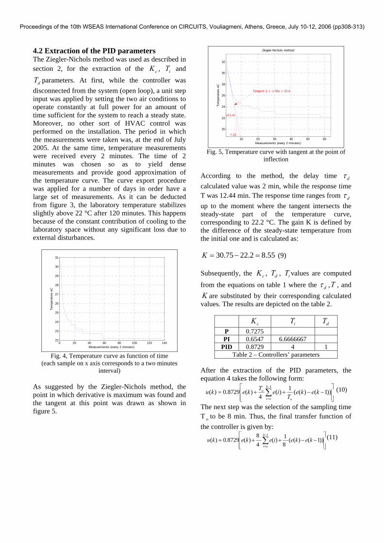
As suggested by the Ziegler-Nichols method, the point in which derivative is maximum was found and the tangent at this point was drawn as shown in figure 5.

10 20 30 40 50 60

20

22

24

26

28

30

32

Measurements (every 2 minutes)

Tem

pera

ture

oC

Ziegler-Nichols method

Tangent: y = -1.55x + 33.4

22.2 oC

7.22

Fig. 5, Temperature curve with tangent at the point of

inflection

According to the method, the delay time dτ calculated value was 2 min, while the response time T was 12.44 min. The response time ranges from dτ up to the moment where the tangent intersects the steady-state part of the temperature curve, corresponding to 22.2 °C. The gain K is defined by the difference of the steady-state temperature from the initial one and is calculated as:

55.82.2275.30 =−=K (9) Subsequently, the , , values are computed from the equations on table 1 where the

cK dT iT

dτ ,T , and are substituted by their corresponding calculated

values. The results are depicted on the table 2. K

cK iT dT P 0.7275 PI 0.6547 6.6666667

PID 0.8729 4 1 Table 2 – Controllers’ parameters

After the extraction of the PID parameters, the equation 4 takes the following form:

⎥⎥⎦

⎤

⎢⎢⎣

⎡−−++= ∑

−

=

1

))1()((1)(4

)(8729.0)(k

oi o

o kekeT

ieTkeku (10)

The next step was the selection of the sampling time T to be 8 min. Thus, the final transfer function of the controller is given by:

o

⎥⎥⎦

⎤

⎢⎢⎣

⎡−−++= ∑

−

=

1

))1()((81)(

48

)(8729.0)(k

oikekeiekeku (11)

Proceedings of the 10th WSEAS International Conference on CIRCUITS, Vouliagmeni, Athens, Greece, July 10-12, 2006 (pp308-313)

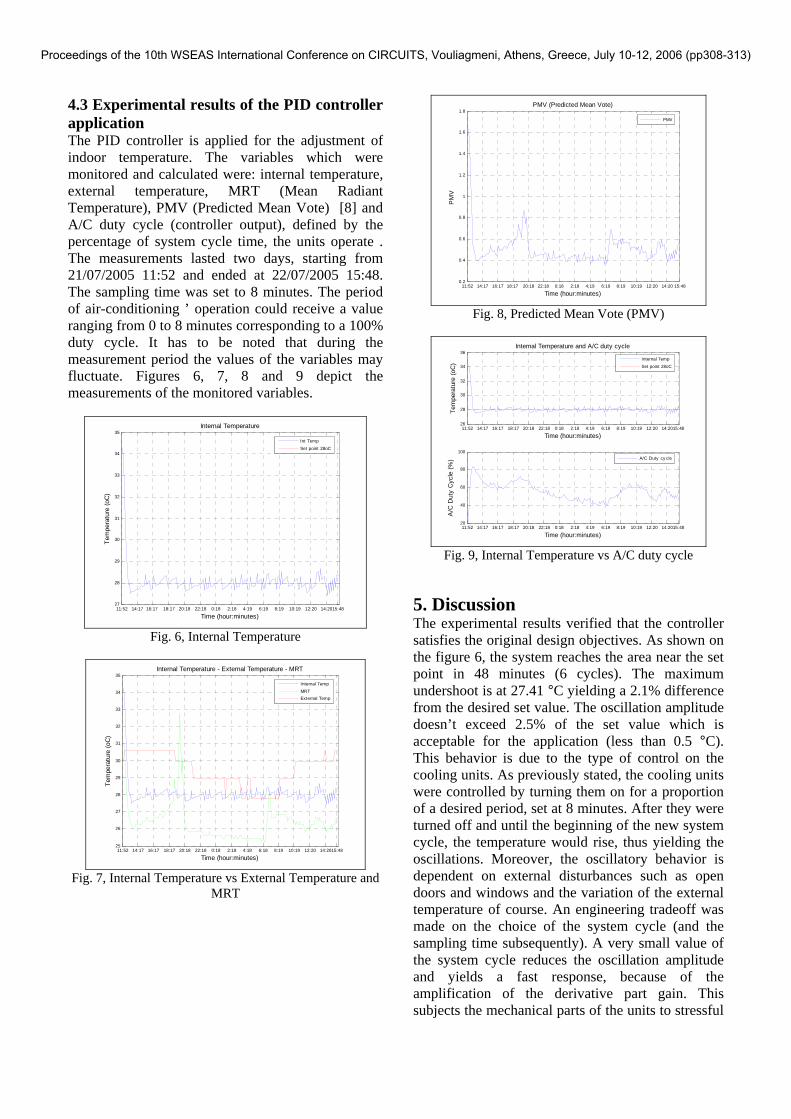
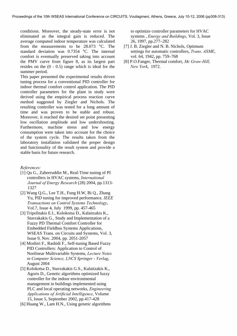
4.3 Experimental results of the PID controller application The PID controller is applied for the adjustment of indoor temperature. The variables which were monitored and calculated were: internal temperature, external temperature, MRT (Mean Radiant Temperature), PMV (Predicted Mean Vote) [8] and A/C duty cycle (controller output), defined by the percentage of system cycle time, the units operate . The measurements lasted two days, starting from 21/07/2005 11:52 and ended at 22/07/2005 15:48. The sampling time was set to 8 minutes. The period of air-conditioning ’ operation could receive a value ranging from 0 to 8 minutes corresponding to a 100% duty cycle. It has to be noted that during the measurement period the values of the variables may fluctuate. Figures 6, 7, 8 and 9 depict the measurements of the monitored variables.

11:52 14:17 16:17 18:17 20:18 22:18 0:18 2:18 4:19 6:19 8:19 10:19 12:20 14:2015:4827

28

29

30

31

32

33

34

35

Time (hour:minutes)

Tem

pera

ture

(oC

)

Internal Temperature

Int TempSet point 28oC

Fig. 6, Internal Temperature

11:52 14:17 16:17 18:17 20:18 22:18 0:18 2:18 4:18 6:18 8:19 10:19 12:20 14:2015:4825

26

27

28

29

30

31

32

33

34

35

Time (hour:minutes)

Tem

pera

ture

(oC

)

Internal Temperature - External Temperature - MRT

Internal TempMRTExternal Temp

Fig. 7, Internal Temperature vs External Temperature and

MRT

11:52 14:17 16:17 18:17 20:18 22:18 0:18 2:18 4;19 6:19 8:19 10:19 12:20 14:20 15:480.2

0.4

0.6

0.8

1

1.2

1.4

1.6

1.8

Time (hour:minutes)

PM

V

PMV (Predicted Mean Vote)

PMV

Fig. 8, Predicted Mean Vote (PMV)

11:52 14:17 16:17 18:17 20:18 22:18 0:18 2:18 4:19 6:19 8:19 10:19 12:20 14:2015:4826

28

30

32

34

36

Time (hour:minutes)

Tem

pera

ture

(oC

)

Internal Temperature and A/C duty cycle

11:52 14:17 16:17 18:17 20:18 22:18 0:18 2:18 4:19 6:19 8:19 10:19 12:20 14:2015:4820

40

60

80

100

Time (hour:minutes)

A/C

Dut

y C

ycle

(%)

Internal TempSet point 28oC

A/C Duty cy cle

Fig. 9, Internal Temperature vs A/C duty cycle

5. Discussion The experimental results verified that the controller satisfies the original design objectives. As shown on the figure 6, the system reaches the area near the set point in 48 minutes (6 cycles). The maximum undershoot is at 27.41 °C yielding a 2.1% difference from the desired set value. The oscillation amplitude doesn’t exceed 2.5% of the set value which is acceptable for the application (less than 0.5 °C). This behavior is due to the type of control on the cooling units. As previously stated, the cooling units were controlled by turning them on for a proportion of a desired period, set at 8 minutes. After they were turned off and until the beginning of the new system cycle, the temperature would rise, thus yielding the oscillations. Moreover, the oscillatory behavior is dependent on external disturbances such as open doors and windows and the variation of the external temperature of course. An engineering tradeoff was made on the choice of the system cycle (and the sampling time subsequently). A very small value of the system cycle reduces the oscillation amplitude and yields a fast response, because of the amplification of the derivative part gain. This subjects the mechanical parts of the units to stressful

Proceedings of the 10th WSEAS International Conference on CIRCUITS, Vouliagmeni, Athens, Greece, July 10-12, 2006 (pp308-313)

conditions. Moreover, the steady-state error is not eliminated as the integral gain is reduced. The average computed indoor temperature was calculated from the measurements to be 28.073 °C. The standard deviation was 0.7354 °C. The internal comfort is eventually preserved taking into account the PMV curve from figure 8, as its largest part resides on the (0 - 0.5) range which is ideal for the summer period. This paper presented the experimental results driven tuning process for a conventional PID controller for indoor thermal comfort control application. The PID controller parameters for the plant in study were derived using the empirical process reaction curve method suggested by Ziegler and Nichols. The resulting controller was tested for a long amount of time and was proven to be stable and robust. Moreover, it reached the desired set point presenting low oscillation amplitude and low undershooting. Furthermore, machine stress and low energy consumption were taken into account for the choice of the system cycle. The results taken from the laboratory installation validated the proper design and functionality of the result system and provide a stable basis for future research. References: [1] Qu G., Zaheeruddin M., Real-Time tuning of PI controllers in HVAC systems, International

Journal of Energy Research (28) 2004, pp.1313-1327

[2] Wang Q.G., Lee T.H., Fung H.W, Bi Q., Zhang Yu, PID tuning for improved performance, IEEE Transactions on Control Systems Technology, Vol.7, Issue 4, July 1999, pp. 457-465

[3] Tripolitakis E.I., Kolokotsa D., Kalaitzakis K., Stavrakakis G., Study and Implementation of a Fuzzy PD Thermal Comfort Controller for Embedded Fieldbus Systems Applications, WSEAS Trans. on Circuits and Systems, Vol. 3, Issue 9, Nov. 2004, pp. 2051-2057

[4] Moshiri F., Rashidi F., Self-tuning Based Fuzzy PID Controllers: Application to Control of Nonlinear Multivariable Systems, Lecture Notes in Computer Science, LNCS Springer - Verlag, August 2004

[5] Kolokotsa D., Stavrakakis G.S., Kalaitzakis K., Agoris D., Genetic algorithms optimized fuzzy controller for the indoor environmental management in buildings implemented using PLC and local operating networks, Engineering Applications of Artificial Intelligence, Volume 15, Issue 5, September 2002, pp.417-428

[6] Huang W., Lam H.N., Using genetic algorithms

to optimize controller parameters for HVAC systems , Energy and Buildings, Vol. 3, Issue 26, 1997, pp.277–282

[7] J. B. Ziegler and N. B. Nichols, Optimum settings for automatic controllers, Trans. ASME, vol. 64, 1942, pp. 759–768

[8] P.O.Fanger, Thermal comfort, Mc Graw-Hill, New York, 1972.

Proceedings of the 10th WSEAS International Conference on CIRCUITS, Vouliagmeni, Athens, Greece, July 10-12, 2006 (pp308-313)