pid controller tuning using bode’s...
TRANSCRIPT
PID Controller Tuning Using Bode’s Integrals ∗
Alireza Karimi, Daniel Garcia and Roland Longchamp †
Abstract
A new method for PID controller tuning based on Bode’s integrals is proposed. It is shown that the
derivatives of amplitude and phase of a plant model with respect to frequency can be approximated
by Bode’s integrals without any model of the plant. This information can be used to design a PID
controller for slope adjustment of the Nyquist diagram and improve the closed-loop performance.
Besides, the derivatives can be also employed to estimate the gradient and the Hessian of a frequency
criterion in an iterative PID controller tuning method. The frequency criterion is defined as the sum of
squared errors between the desired and measured gain margin, phase margin and crossover frequency.
The method benefits from specific feedback relay tests to determine the gain margin, the phase margin
and the crossover frequency of the closed-loop system. Simulation examples and experimental results
illustrate the effectiveness and the simplicity of the proposed method to design and tune the PID
controllers.
Keywords: PID controller, relay feedback test, phase margin, gain margin, autotuning
1 Introduction
PID controllers are widely used in industrial plants and different methods for the design or the tuning of
these controllers have been proposed in the literature [8, 16, 3]. The available methods are normally based
on a first or a second-order model with time delay obtained from the time response or the measurement of
multiple points on the frequency response of the process. The specifications are often expressed in terms
of phase and/or gain margins [7, 12, 6], because they are the classical measures of robustness and together
with the crossover frequency, they represent the time domain performance of the closed-loop system as well.
This problem, in general, even if the plant model is perfectly known, leads to a set of nonlinear equations for
which no analytic solution is available. The traditional methods are the graphical algorithms using Bode
plots which are not very suitable for autotuning of the PID controllers. More advanced methods try either
to find a solution by numerical methods [12] or to simplify the equations using some approximations to
∗This research work is financially supported by the Swiss National Science Foundation under grant No. 2100-064931.01†The authors are with the Laboratoire d’Automatique, Ecole Polytechnique Federale de Lausanne (EPFL), 1015 Lausanne,
Switzerland. (email: [email protected])
1

find an analytic solution [6]. The main drawback of these approaches is that the desired specifications are
not necessarily achieved on the real system because of the approximations in modeling and/or equations.
In addition, they do not lead to on-line tuning methods in order to meet the specifications for the real
plant.
In 1984, Astrom and Hagglund [7] proposed an automatic tuning method based on a simple relay
feedback test which gives, using the describing function analysis, the critical gain and the critical frequency
of the system. Other points on the Nyquist curve can be identified using a relay with hysteresis [7] or by
introducing an adjustable time delay in the closed-loop system [10, 1]. A closed-loop relay test scheme
was proposed in [15] which identifies directly the crossover frequency (the frequency at which the loop
gain is equal to 1). After identifying a point on the frequency response of the plant, the so-called modified
Ziegler-Nichols method can be used to move this point to another position in the complex plane [8]. Two
equations for phase and amplitude assignment are obtained which can be solved to find the parameters of
a PI or PD controller. For a PID controller, however, an additional equation should be introduced. In the
modified Ziegler-Nichols method, the ratio between integral time Ti and derivative time Td is chosen to be
constant (Ti = 4Td) in order to have a unique solution. In a recent paper [9], it is shown that Ti = 2.5Td
gives better results than the classical choice for a certain number of plant models. In [8], it was proposed
finding the relation between Ti and Td assuring a desired slope for the Nyquist curve of the loop transfer
function at a given frequency. However, this relation depends inevitably on the derivatives of the plant
transfer function with respect to frequency which are not known a priori.
The main contribution of this paper is in the use of Bode’s integrals for PID controller tuning. The
Bode’s integrals [2] show the relation between the phase and the amplitude of minimum phase stable
systems. It will be shown how these integrals can be used to approximate the derivatives of the amplitude
and the phase of a system with respect to frequency at a given frequency. It is interesting to notice that
the approximation is made only with the knowledge of the amplitude and the phase of the system at the
given frequency and the system static gain. As a result, with a simple relay test, not only are the phase
margin and the crossover frequency identified, but also the derivatives of the plant transfer function at
crossover frequency are approximated with no parametric model of the plant. The derivatives can be used
in the modified Ziegler-Nichols method to adjust the slope of the Nyquist curve at the crossover frequency.
They can also be employed in an autotuning scheme for computing the gradient and the Hessian of a
frequency criterion which is minimized iteratively. The frequency criterion can be defined as the sum of
squared normalized errors between the desired and measured gain margin, phase margin and crossover
frequency. An advantage compared with the autotuning methods based on a time criterion is that in each
iteration a robustness margin is measured which can be used to make a stability test before applying the
new controller to the system.
An iterative procedure for gain and phase margin adjustment for a PI controller was presented in [4].
The approach uses similar relay tests, but the gradient of the criterion is not calculated and an ad hoc
2

algorithm is used, instead. As a result the algorithm converges much slower than the proposed method.
The paper is organized as follows: In Section 2 several relay feedback tests will be briefly reviewed. Sec-
tion 3 shows how the Bode’s integrals can be employed for slope adjustment in the modified Ziegler-Nichols
method. An iterative tuning method for gain and phase margin adjustment together with simulation ex-
amples are presented in Section 4. An application of the proposed method to a three-tank system in
Section 5 shows the effectiveness and fast convergence of the iterative method. Finally, Section 6 gives
some concluding remarks.
2 Relay feedback test
The relay method is a well-known technique to identify useful points on the Nyquist curve by generating
an appropriate oscillation with a relay feedback. In the standard relay method the controller is replaced
by an on-off relay in closed-loop. For many systems there will be an oscillation when the control signal is
a square wave and the process output is close to a sinusoid. The amplitude and the frequency of the limit
cycle obtained give, respectively, the point where the Nyquist curve intersects the negative real axis and
its corresponding frequency.
Relay feedback can also be applied to closed-loop systems including a linear controller. Fig. 1 shows an
experiment where the output of the relay is the reference signal for the closed-loop system with an existing
controller K(s) and the output of the closed-loop system is fed back to the relay input. The identified
0
_ _
d
-dK(s)G(s)
Figure 1: Relay experiment for gain margin measurement
point, obtained from the amplitude of the limit cycle, is on the intersection of the open-loop Nyquist curve
with the segment (−1, 0). The gain margin is defined as the inverse of the amplitude of the identified
point.
The experiment proposed in [15] and shown in Fig. 2 generates a limit cycle at the crossover frequency
of the open-loop transfer function K(jω)G(jω). The phase margin can be approximated by the amplitude
and frequency of the generated limit cycle [11]. Let ωc be the measured limit cycle frequency (equal to
the crossover frequency), ac the relay input amplitude and d the relay output amplitude. Then the phase
of the identified point can be computed as follows:
� K(jωc)G(jωc) = −2 arctan(πacωc
4d)
3

0
__
_
2
1s
d
-dK(s)G(s)
Figure 2: Relay experiment for phase margin measurement
The phase margin Ψ is then given by
Ψ = π − 2 arctan(πacωc
4d).
The proposed methods for measuring the gain and phase margins by the relay method have the draw-
back that the method of the describing function must be used for the identification of the frequencies and
the points on the Nyquist curve of interest. This approach is approximative. Several methods are proposed
to improve the precision of the approximations [16]. In this paper, an adaptive identification method to
the critical gain proposed in [14] is used in all of the simulation examples and experiments. In this method
the relay is replaced by a saturation nonlinearity and a time varying gain.
3 Loop slope adjustment using Bode’s integrals
The slope of the Nyquist curve at the crossover frequency affects drastically the performance and robustness
of the closed-loop system. In this section, first a formula is derived which gives the relation between Ti and
Td for obtaining the desired slope of the Nyquist curve of the loop transfer function at a given frequency.
Then the Bode’s integrals are used to approximate the derivatives of the plant transfer function. Finally, the
parameters of a PID controller for the desired phase margin and slope at a given frequency are determined.
3.1 Loop slope adjustment
Consider the loop transfer function L(jω) = G(jω)K(jω) where
K(jω) = Kp(1 +1
jωTi+ jωTd) (1)
is the PID controller. The slope of the Nyquist curve of the loop transfer function L(jω) at ω0 defined by
ψ is equal to the phase of the derivative of L(jω) at ω0. The derivative of the loop transfer function with
respect to ω is computed as follows:
dL(jω)dω
= G(jω)dK(jω)dω
+K(jω)dG(jω)dω
(2)
Furthermore one has:
lnG(jω) = ln |G(jω)|+ j � G(jω) (3)
4

Differentiating this equation gives:
d lnG(jω)dω
=1
G(jω)dG(jω)dω
=d ln |G(jω)|
dω+ j
d � G(jω)dω
(4)
On the other hand, the derivative of the controller with respect to ω is:
dK(jω)dω
= jKp(Td +1
ω2Ti) (5)
Substituting Eqs (1), (4) and (5) into Eq. (2), one obtains:
dL(jω)dω
= KpG(jω)[j(Td +
1ω2Ti
) +(
1 + j(Tdω −1ωTi
)) (
d ln |G(jω)|dω
+ jd � G(jω)
dω
)](6)
Hence, the slope of the Nyquist curve at ω0 is given by:
ψ = � dL(jω)dω
∣∣∣∣ω0
= ϕ0 + arctan(TdTiω2
0 + 1) + (TdTiω20 − 1)sa(ω0) + sp(ω0)Tiω0
sa(ω0)Tiω0 − (TdTiω20 − 1)sp(ω0)
(7)
where ϕ0 = � G(jω0) and sa(ω0) and sp(ω0) are defined as follows:
sa(ω0) = ω0d ln |G(jω)|
dω
∣∣∣∣ω0
(8)
sp(ω0) = ω0d � G(jω)
dω
∣∣∣∣ω0
(9)
It is desired to adjust the slope of the Nyquist curve of the loop transfer function L(jω) to a specified
value ψ. Then straightforward calculation gives:
Td =sa(ω0)− 1 + sp(ω0) tan(ψ − ϕ0)− Tiω0(sp(ω0)− sa(ω0) tan(ψ − ϕ0))
ω20Ti(1 + sa(ω0) + sp(ω0) tan(ψ − ϕ0))
(10)
In the next part, sa(ω0) and sp(ω0) are directly approximated using the Bode’s integrals.
3.2 Bode’s integrals
The relations between the phase and the amplitude of a stable minimum-phase system have been inves-
tigated for the first time by Bode [2]. The results are based on Cauchy’s residue theorem and have been
extensively used in network analysis. Two integrals are presented in this section. The first one, which
is well known in the control engineering field, shows the relationship between the phase of the system at
each frequency as a function of the derivative of its amplitude. But the second integral, to the best of the
authors’ knowledge, has been never used in the control design. The integral shows how the amplitude of
the system at each frequency is related to the derivative of the phase and the static gain of the system.
3.2.1 Derivative of amplitude
Bode has shown in [2] that for a stable minimum-phase transfer function G(jω), the phase of the system
at ω0 is given by:
� G(jω0) =1π
∫ +∞
−∞
d ln |G(jω)|dν
ln coth|ν|2dν (11)
5

where ν = ln ωω0
. Since ln coth |ν|2 decreases rapidly as ω deviates from ω0, the integral depends mostly ond ln |G(jω)|
dν (the slope of the Bode plot) near ω0. Therefore, assuming that the slope of the Bode plot is
almost constant in the neighborhood of ω0, � G(jω0) can be approximated by:
� G(jω0) ≈1π
d ln |G(jω)|dν
∣∣∣∣ω0
∫ +∞
−∞ln coth
|ν|2dν =
π
2d ln |G(jω)|
dν
∣∣∣∣ω0
(12)
This property is often used in loop shaping where the slope of the amplitude Bode plot at the crossover
frequency is limited to -20dB/decade in order to obtain approximately a phase margin of 90◦. Here the
measured phase of the system at ω0 is used to determine approximately the slope of the amplitude Bode
plot (sa):
sa(ω0) =d ln |G(jω)|
dν
∣∣∣∣ω0
= ω0d ln |G(jω)|
dω
∣∣∣∣ω0
≈ 2π� G(jω0) (13)
3.2.2 Derivative of phase
The second Bode’s integral shows that the amplitude of a stable minimum-phase system can be determined
uniquely from its phase and its static gain. More precisely, the logarithm of the system amplitude at ω0
is given by [2]:
ln |G(jω0)| = ln |Kg| −ω0
π
∫ +∞
−∞
d(� G(jω)/ω)dν
ln coth|ν|2dν (14)
where Kg is the static gain of the plant. In the same way, assuming that � G(jω)/ω is linear (in a
logarithmic scale) in the neighborhood of ω0, one has:
ln |G(jω0)| ≈ ln |Kg| −ω0
π
d(� G(jω)/ω)dν
∣∣∣∣ω0
π2
2(15)
ln |G(jω0)| ≈ ln |Kg| −πω2
0
2
[1ω0
d � G(jω)dω
∣∣∣∣ω0
−� G(jω0)
ω20
](16)
which gives:
sp(ω0) = ω0d � G(jω)
dω
∣∣∣∣ω0
≈ � G(jω0) +2π
[ln |Kg| − ln |G(jω0)|] (17)
Note that for the systems containing an integrator, the static gain cannot be computed. For such
systems, the static gain of the system without the integrator should be estimated and used in the above
formula (note that the phase of the integrator is constant and its derivative is zero).
3.2.3 Precision of the estimates
The precision of the estimates of the derivatives of amplitude and phase depends on the system dynamics
and on the frequency at which the experiments are performed. However, extensive simulations on the
typical models of industrial plants have shown that the absolute normalized error of the estimates is in
an acceptable range. In order to give an idea about the precision of the estimates, let us consider the
following system:
G(s) =1
(s+ 1)n(18)
6

where n is a positive integer. The true values of sa(ω) and sp(ω)/ω computed on the basis of the model
for different frequencies, are compared with the estimated ones based on the Bode’s integrals in Fig. 3
and Fig. 4, respectively. It can be observed that the maximum of the absolute normalized error does not
exceed 0.1 for this system.
10-2
10-1
100
101
102
-n
-n/2
0
Frequency [rad/s]
sa(ω)
Figure 3: Comparison of true sa(ω) and the estimated one based on Bode’s integral (solid line: true values,
dashed line: estimates )
10-2
10-1
100
101
102
-n
-n/2
0
Frequency [rad/s]
sp(ω)/ω
Figure 4: Comparison of true sp(ω)/ω and the estimated one based on Bode’s integral (solid line: true
values, dashed line: estimates )
Similar results can be obtained for the systems presented by several first-order models in cascade. For
oscillatory systems, the estimation may be poor in certain frequencies, but in general the results remain
satisfactory. For non-minimum-phase systems the Bode’s integrals are no longer valid and the proposed
formulas give incorrect results. However, it will be shown next that the pure time delay has no effect on
the estimation of sp and its effect on the estimation of sa can be neglected if it is small with respect to
7

the dominant time constant of the system.
3.2.4 Effect of pure time delay
Consider the following system with a pure time delay τ :
Gτ (jω) = G(jω)e−jτω (19)
where G(jω) is a stable minimum-phase system. Differentiating the amplitude and phase of Gτ (jω) with
respect to ω gives:
d ln |Gτ (jω)|dω
=d ln |G(jω)|
dω,
d � Gτ (jω)dω
=d � G(jω)
dω− τ
Now using the Bode’s integral from Eq. (12), the phase of Gτ (jω) at ω0 is approximated by:
� Gτ (jω0) = � G(jω0)− τω0 ≈π
2d ln |G(jω)|
dω
∣∣∣∣ω0
− τω0 (20)
Then sa(ω0) and sp(ω0) for a system including a pure time delay are computed as follows:
sa(ω0) = ω0d ln |Gτ (jω)|
dω
∣∣∣∣ω0
≈ 2π
(� Gτ (jω0) + τω0) (21)
sp(ω0) = ω0d � Gτ (jω)
dω
∣∣∣∣ω0
= ω0d � G(jω)
dω
∣∣∣∣ω0
− τω0 ≈ � G(jω0) +2π
[ln |Kg| − ln |G(jω0)|]− τω0
≈ � Gτ (jω0) +2π
[ln |Kg| − ln |Gτ (jω0)|] (22)
The above relations show that the pure time delay should be known for the calculation of sa(ω0) but it
has no effect on the calculation of sp(ω0). It should be remembered that τ represents the pure time delay
of the system which is usually related to the mass transport delay and is often negligible or can be easily
measured. This value should not be confounded with the time delay that is used to model a high-order
system as a first- or second-order system with delay. For example, G(s) = 1/(s + 1)5 has no pure time
delay whereas it can be approximated by a first-order model with a large time delay.
3.3 PID design
Suppose that the amplitude and the phase of a plant at the crossover frequency ωc are known. These
values may be obtained using the existing controller and by the method mentioned in Section 2. Suppose
also that the static gain of the process is measured. The objective is to improve the controller performance
by adjusting the phase margin and the slope of the Nyquist curve at the crossover frequency. The modified
Ziegler-Nichols method is used but the derivatives are approximated by the Bode’s integrals, so no model
for the system is required. To obtain a desired phase margin Φd at the crossover frequency ωc we have the
following equations to solve:
� G(jωc) + � K(jωc) = Φd − π (23)
|G(jωc)K(jωc)| = 1 (24)
8

Solving these equations one obtains:
Kp =cos(Φd − ϕc − π)|G(jωc)|
(25)
Tdωc −1
Tiωc= tan(Φd − ϕc) (26)
where ϕc is the phase of G(jωc). Now we exploit Eq. (10) in order to obtain the desired slope ψ at
the crossover frequency. Combining Eqs (10) and (26), we obtain after straightforward calculations the
parameters Ti and Td as follows:
Ti =1
ωc(Tdωc − tan(Φd − ϕc))(27)
Td =1
2ωc[(sa(ωc)− sp(ωc) tan(Φd − ϕc)) tan(ψ − ϕc) + (1− sa(ωc)) tan(Φd − ϕc)− sp(ωc)] (28)
The improved PID controller is now defined by (25), (27) and (28).
3.4 Example
The PID design method presented above will be illustrated by the following simulation model:
G(s) =1
(s+ 1)5(29)
The specifications are set at 0.4 rad/s for the crossover frequency and 50◦ for the phase margin. First, the
control parameters are obtained using the modified Ziegler-Nichols method. The resulting PID controller
is
K(s) = 1.35 (1 +1
3.44s+ 0.86s) (30)
This controller moves the point G(0.4 j) of the Nyquist curve to a point of K(jω)G(jω) on the unit circle
having a phase of 130◦. This conforms to the closed-loop system with the specifications mentioned above.
In order to improve the closed-loop performance, let us calculate now a controller that provides the
closed-loop system the same crossover frequency and phase margin, but with the desired slope of the open-
loop Nyquist curve at the crossover frequency of 65◦. This reduces the current slope of the Nyquist curve
by 25◦ and ensures a greater distance of the Nyquist curve from the critical point in high frequencies.
The controller parameters are obtained from Eqs (25), (28) and (27), where sa(0.4 j) and sp(0.4 j) are
approximated using Eqs (13) and (17):
K(s) = 1.35 (1 +1
2.81s+ 1.27s) (31)
Although the approximation error for sa and sp leads to a resultant slope of 74◦ (about 13% error), a
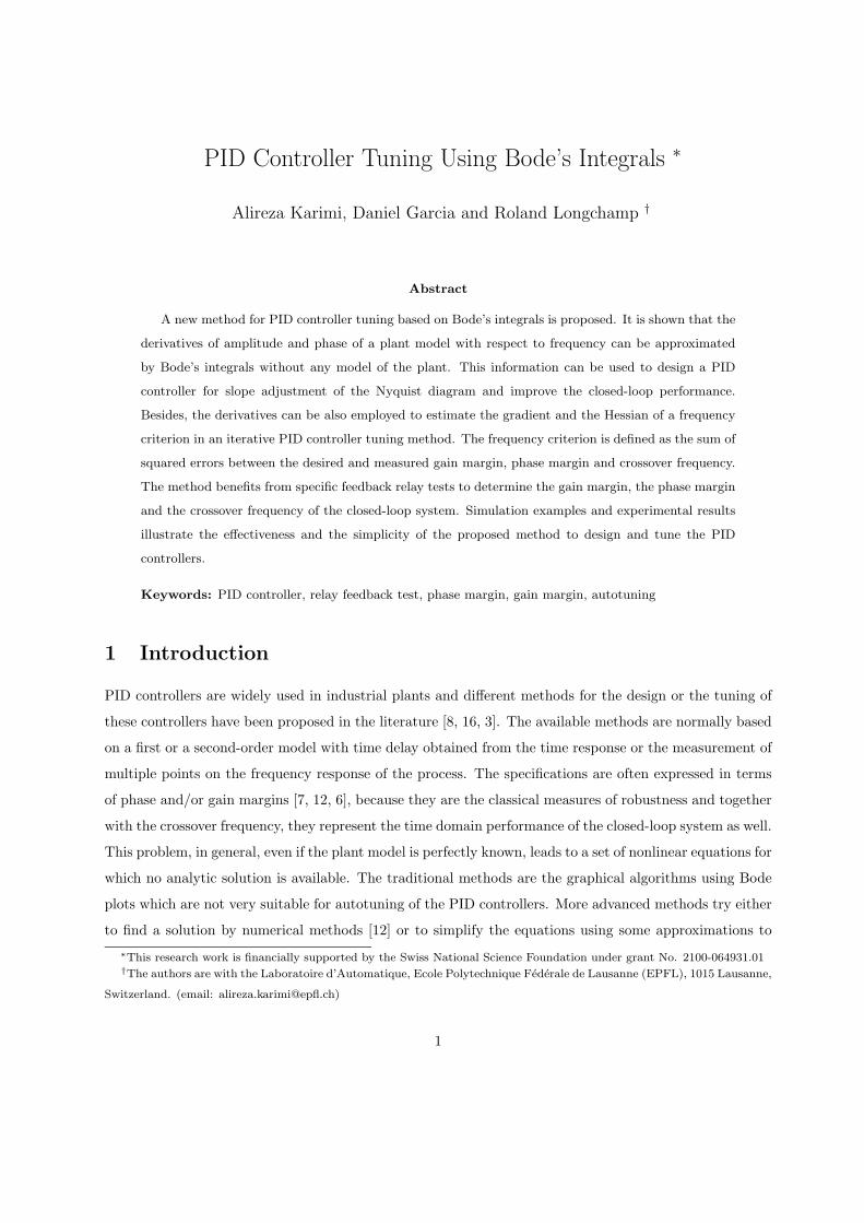
comparison of the closed-loop performance for the two controllers shown in Fig. 5 illustrates a significant
improvement of the closed-loop performance. The overshoot is about the same but the settling time is
44 % smaller with the proposed method. it should be mentioned that, in the simulation, the derivative
9
part of the ideal PID controller is replaced by a causal derivator Tds1+Td/20s
and no saturation is considered
for the control signal. The Nyquist diagrams (Fig. 6) further show that the proposed controller modifies
the slope of the Nyquist curve and as a result improves the gain margin as well as the modulus margin
(the minimum distance between L(jω) and the critical point) of the system.
0 5 10 15 20 250
0.2
0.4
0.6
0.8
1
1.2
Time [s]
Step response
0 5 10 15 20 250.5
1
1.5
2
2.5
3
Time [s]
Control signal
Figure 5: Step response of the closed-loop system (dashed line: modified Ziegler-Nichols, solid line: pro-
posed)
4 Iterative PID tuning in closed-loop
In the previous section, it was assumed that the amplitude and the phase of the plant at the crossover
frequency are known or they are measured by a relay feedback experiment with an existing controller.
However, if the desired crossover frequency is different from the measured one, an analytic solution as
presented in the previous section cannot be obtained. Therefore it is not possible, for example, to improve
the performance of the closed-loop system by increasing the crossover frequency which is closely related
to closed-loop bandwidth. In addition, although the Nyquist curve of the loop transfer function passes
10

-1 -0.5 0 0.5-1.5
-1
-0.5
0
Real axis
Imag
inar
y ax
is
Nyquist diagram
Figure 6: Nyquist diagram (dashed line: modified Ziegler-Nichols, solid line: proposed)
through a point with the desired phase, it is not guaranteed that this point gives the phase margin (it is
possible that the Nyquist curve intersects several times the unit circle). So an extra relay feedback test
using the new controller should be carried out in order to validate the desired performance on the real
system.
In this section an iterative tuning method in the frequency domain is proposed. The method is based
on the measurement of the phase margin and the crossover frequency by the closed-loop relay test of
Section 2 improved by an adaptive gain adjustment proposed in [14]. In this method, a frequency criterion
is minimized iteratively using the Gauss-Newton algorithm. The particularity of this method is that the
gradient of the criterion is approximated using the Bode’s integrals and no model of the plant is required.
4.1 Iterative procedure for phase margin adjustment
First of all, a performance criterion in the frequency domain is defined as follows:
J(ρ) =12[(ωc − ωdωd
)2 + (Φm − Φd
Φd)2] (32)
where ρ is the vector of the controller parameters, ωc and ωd are respectively the measured and desired
crossover frequencies, and Φm and Φd are the measured and desired phase margins. The error between
the measured and the desired values are normalized in order that the same weighting for each variable in
the criterion to be obtained. This avoids the numerical problems in the iterative algorithm. In the next
step, the controller parameters minimizing the criterion are obtained by the iterative Newton formula:
ρi+1 = ρi − γiR−1J ′(ρi) (33)
11
where i is the iteration number, γi is a positive scalar representing the step size, R is a square positive
definite matrix of dimension ρ and J ′(ρ) is the gradient of the criterion with respect to ρ. This algorithm
converges to the vector of parameters minimizing the criterion, provided that the step size is properly
chosen [5]. The matrix R can be chosen equal to the identity matrix or to the Hessian of the criterion to
obtain faster convergence (Gauss-Newton method).
It should be mentioned that the slope of the loop Nyquist curve can also be adjusted simultaneously
in the iterative approach. In fact, in this case, the vector of parameters contains only Kp and Ti and Eq.
(10) is used at each iteration to compute Td.
The gradient of the criterion is given by:
J ′(ρ) =1ω2d
(ωc − ωd)∂ωc∂ρ
+1
Φ2d
(Φm − Φd)Φ′m (34)
where Φ′m is the derivative of the phase margin with respect to ρ computed through the chain rule (note
that Φm is a function of ρ and ωc):
Φ′m =∂Φm∂ρ
+∂Φm∂ω
∣∣∣∣ωc
∂ωc∂ρ
(35)
Now replacing Φm in the above equation by � L(jωc) + π gives:
Φ′m =∂ � L(jωc)
∂ρ+∂ � L(jω)∂ω
∣∣∣∣ωc
∂ωc∂ρ
(36)
The first term in the above equation is equal to ∂ � K(jωc)/∂ρ which is completely known at each iteration.
Furthermore one has:
∂ � L(jω)∂ω
∣∣∣∣ωc
=∂ � K(jω)
∂ω
∣∣∣∣ωc
+∂ � G(jω)
∂ω
∣∣∣∣ωc
=∂ � K(jω)
∂ω
∣∣∣∣ωc
+sp(ωc)ωc
(37)
Again, the first term is completely known and sp(ωc) can be approximated using Eq. (17). Now, it only
remains to compute ∂ωc/∂ρ. For this purpose, we use the fact that the loop gain at ωc in each iteration
is equal to 1, therefore its derivative (or derivative of its logarithm) with respect to ρ will be zero. Then
one has:∂ ln |L(jωc)|
∂ρ+∂ ln |L(jω)|
∂ω
∣∣∣∣ωc
∂ωc∂ρ
= 0 (38)
but from the Bode’s integral (see Eq. (13)) one has:
∂ ln |L(jω)|∂ω
∣∣∣∣ωc
≈ 2 � L(jωc)πωc
=2(Φm − π)
πωc(39)
Thus ∂ωc/∂ρ can be approximated as follows (note that ∂ ln |L(jω)|/∂ρ = ∂ ln |K(jω)|/∂ρ):
∂ωc∂ρ≈ − πωc
2(Φm − π)∂ ln |K(jωc)|
∂ρ(40)
Notice that the gradient of the criterion is computed using only the measured crossover frequency ωc and
the measured amplitude and phase of the plant. In the same way, the Hessian of the criterion can be
12

approximated without any additional information as follows:
H = J ′′(ρ) =1ω2d
∂ωc∂ρ
(∂ωc∂ρ
)T +1
Φ2d
Φ′m(Φ′m)T +1ω2d
(ωc − ωd)∂2ωc∂ρ2
+1
Φ2d
(Φm − Φd)Φ′′m (41)
The last two terms can be neglected because they are small especially in the neighborhood of the final
solution. In addition, this simplification makes the Hessian always positive which fixes the numerical
problems normally encountered in the iterative Newton algorithm. The use of the Hessian matrix in the
iterative formula (Eq. 33) instead of R significantly improves the convergence speed.
R = H ≈ 1ω2d
∂ωc∂ρ
(∂ωc∂ρ
)T +1
Φ2d
Φ′m(Φ′m)T (42)
4.2 Iterative procedure for phase and gain margins adjustment
In phase margin and slope adjustment, the controller is designed using only the information on one fre-
quency point of the plant. Although this approach is very fast and simple and works well for the majority
of the industrial processes, it may not work appropriately for some complex high-order systems. This
means that the specifications may be satisfied just locally at the crossover frequency and it is possible that
the behavior of the system changes drastically elsewhere, leading for example to a very small gain margin.
For such systems, it may be preferable to tune the phase and gain margins at the same time. However,
this necessitates two relay experiments in each iteration: one relay test to measure the gain margin and
the other for the phase margin. A frequency criterion can be defined as follows:
J(ρ) =12[(ωc − ωdωd
)2 + (Φm − Φd
Φd)2 + (
Ku −Kd
Kd)2] (43)
where Ku = |L(jωu)| is the amplitude of the loop transfer function where it intersects the negative real
axis (� L(jωu) = −π). ωu is the critical loop frequency, Kd is the inverse of the desired gain margin. The
gradient of the criterion is given by:
J ′(ρ) =1ω2d
(ωc − ωd)∂ωc∂ρ
+1
Φ2d
(Φm − Φd)Φ′m +1K2d
(Ku −Kd)K ′u (44)
where K ′u is the derivative of the critical loop gain with respect to ρ computed as follows:
K ′u =∂|L(jωu)|
∂ρ+∂|L(jω)|∂ω
∣∣∣∣ωu
∂ωu∂ρ
(45)
The first term is equal to |G(jωu)| · ∂|K(jωu)|/∂ρ which can be easily computed at each iteration. The
second term can be approximated using the Bode’s integrals in a similar way as is done for the phase
margin. First the derivative of the amplitude of the loop gain is computed using Eq. (13) as follows:
∂|L(jω)|∂ω
∣∣∣∣ωu
= |L(jωu)|∂ ln |L(jω)|
∂ω
∣∣∣∣ωu
≈ Ku2� L(jωu)πωu
= −2Ku
ωu(46)
Then ∂ωu/∂ρ is computed using the fact that in each iteration � L(jωu) = −π and consequently its
derivative with respect to ρ will be zero, which gives:
∂ � L(jωu)∂ρ
+∂ � L(jω)∂ω
∣∣∣∣ωu
∂ωu∂ρ
= 0 (47)
13
The first term in the above equation is equal to ∂ � K(jωu)/∂ρ which can be computed knowing the
controller at each iteration. Furthermore one has:
∂ � L(jω)∂ω
∣∣∣∣ωu
=∂ � K(jω)
∂ω
∣∣∣∣ωu
+∂ � G(jω)
∂ω
∣∣∣∣ωu
(48)
Again, knowing the controller at each iteration, the first term in the right hand side can be computed
while the second term is approximated using the Bode’s integral of Eq. (17). Therefore ∂ωu/∂ρ is given
by:
∂ωu∂ρ
= −(∂ � K(jω)
∂ω
∣∣∣∣ωu
+sp(ωu)ωu
)−1∂ � K(jωu)
∂ρ(49)
In a similar way an approximation of the Hessian can also be computed as follows:
R = H ≈ 1ω2d
∂ωc∂ρ
(∂ωc∂ρ
)T +1
Φ2d
Φ′m(Φ′m)T +1K2d
K ′u(K′u)T (50)
4.3 Simulation example
Now let us consider a complex plant model including a time delay as follows:
G(s) =e−0.3s
(s2 + 2s+ 3)3(s+ 3)(51)
This model was proposed in [13] and represents a difficult problem to be solved using a PID controller. It
should be noted that neither the traditional Ziegler-Nichols method nor a more advanced method based
on a first-order plant model [6] can give a stabilizing controller for this plant. Contrary to the simulation
example presented in Section 3.4, it is very difficult here to tune a controller using the slope adjustment
method, because a little change in the slope of the Nyquist curve at the crossover frequency may even make
the closed-loop system unstable. In the following, it is shown that a controller which confers appropriate
specifications on the closed-loop system can be tuned with the iterative phase and gain margins adjustment
method. This method requires two experiments per iteration and is more convenient for high-order complex
systems. However, one should note that the experimental time for the gain margin measurement can be
chosen to be smaller than that of the phase margin, because the critical frequency is appreciably larger
than the crossover frequency.
The specifications are set for this example at ωd = 0.2 rad/s for the crossover frequency, and Φd = 70◦
and Kd = 13 for the phase and for the inverse of the gain margin, respectively. The initial controller is
designed using the Kappa-Tau tuning rule proposed in [8] which gives the following stabilizing controller:
K(s) = 4.5 (1 +1
0.41s+ 0.033s) (52)
The performance criterion of Eq. (43) is considered. Two closed-loop experiments are performed to
measure a crossover frequency of 0.139 rad/s, a phase margin of 78.5◦ and a gain margin of 4.39, which
14

give a performance criterion of 0.104. With these values, the gradient and Hessian are calculated, and a
new controller is obtained. After one other iteration the following controller is obtained:
K(s) = 4.93 (1 +1
0.316s+ 0.125s) (53)
with a performance criterion of 0.0017. This controller gives 0.1997 rad/s for the crossover frequency, 66.0◦
for the phase margin and 2.97 for the gain margin. It should be noted that no significant improvement
can be achieved with further iterations. A comparison of the closed-loop performance between the initial
controller and the final one in Fig. 7 shows that a much smaller settling time is achieved with an overshoot
of only 0.7 %. In the simulation example, Tds is replaced by a causal derivator Tds1+Td/20s
.
0 10 20 30 400
0.2
0.4
0.6
0.8
1
Time [s]
Step response
0 10 20 30 400
20
40
60
80
Time [s]
Control signal
Figure 7: Step response of the closed-loop system (dashed line: Kappa-Tau, solid line: proposed)
It is worth mentioning that even if the estimation errors of sa might be large due to the presence of an
unknown pure time delay in the plant model, the criterion converges rapidly enough. The reason is that
in the Gauss-Newton algorithm the quadratic criterion will converge to its minimum value even with an
approximative gradient.
15
5 Real-time experiment
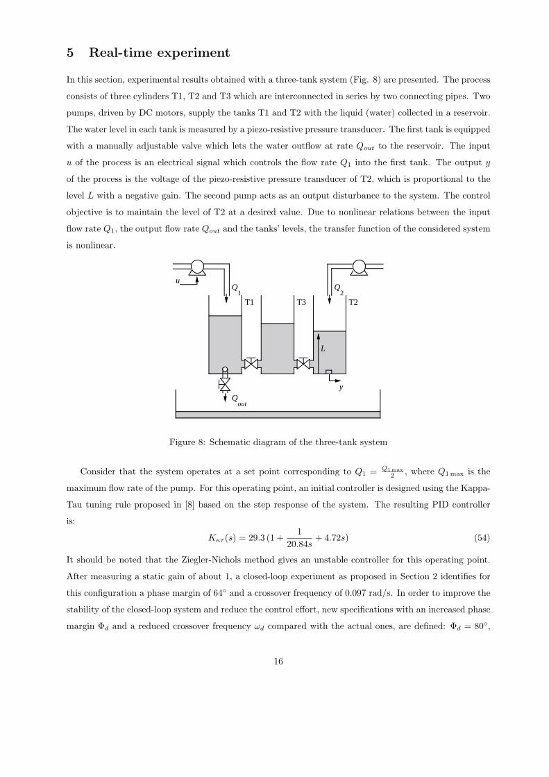
In this section, experimental results obtained with a three-tank system (Fig. 8) are presented. The process
consists of three cylinders T1, T2 and T3 which are interconnected in series by two connecting pipes. Two
pumps, driven by DC motors, supply the tanks T1 and T2 with the liquid (water) collected in a reservoir.
The water level in each tank is measured by a piezo-resistive pressure transducer. The first tank is equipped
with a manually adjustable valve which lets the water outflow at rate Qout to the reservoir. The input
u of the process is an electrical signal which controls the flow rate Q1 into the first tank. The output y
of the process is the voltage of the piezo-resistive pressure transducer of T2, which is proportional to the
level L with a negative gain. The second pump acts as an output disturbance to the system. The control
objective is to maintain the level of T2 at a desired value. Due to nonlinear relations between the input
flow rate Q1, the output flow rate Qout and the tanks’ levels, the transfer function of the considered system
is nonlinear.
Q1
Q2
Qout
T3 T2T1
u
y
L
Figure 8: Schematic diagram of the three-tank system
Consider that the system operates at a set point corresponding to Q1 = Q1 max2 , where Q1 max is the
maximum flow rate of the pump. For this operating point, an initial controller is designed using the Kappa-
Tau tuning rule proposed in [8] based on the step response of the system. The resulting PID controller
is:
Kκτ (s) = 29.3 (1 +1
20.84s+ 4.72s) (54)
It should be noted that the Ziegler-Nichols method gives an unstable controller for this operating point.
After measuring a static gain of about 1, a closed-loop experiment as proposed in Section 2 identifies for
this configuration a phase margin of 64◦ and a crossover frequency of 0.097 rad/s. In order to improve the
stability of the closed-loop system and reduce the control effort, new specifications with an increased phase
margin Φd and a reduced crossover frequency ωd compared with the actual ones, are defined: Φd = 80◦,
16

ωd = 0.08 rad/s. As another specification, a desired value for the slope of the Nyquist curve at crossover
frequency or a constant ratio between the integral time and the derivative time should be considered. In
this experiment, like in the classical Ziegler-Nichols, Ti = 4Td is considered and the derivative part of the
controller is replaced by a causal derivator Tds1+Td/20s
. In the next step the gradient and the Hessian are
calculated and a new controller is obtained after the first iteration:
K(s) = 20.4 (1 +1
31.5s+ 7.88s) (55)
The closed-loop test applied to the system with the controller in Eq.(55) gives the following estimates:
Φm = 86.2◦ ωm = 0.085rad/s
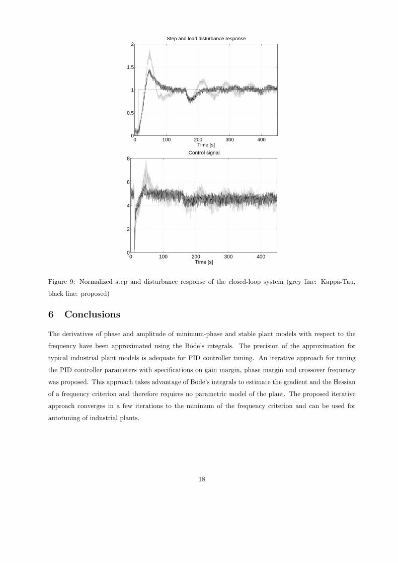
As the estimated values are close to the desired ones, there is no need for further iterations. A comparison
between the time response of the closed-loop system with the Kappa-Tau controller and the proposed one
is shown in Fig. 9. The step response is normalized and the output disturbance concerns a constant flow
rate Q2 for the pump 2 applied at t = 160s. It can be seen that the proposed controller gives a much better
performance for the closed-loop system in terms of disturbance rejection, overshoot and settling time.
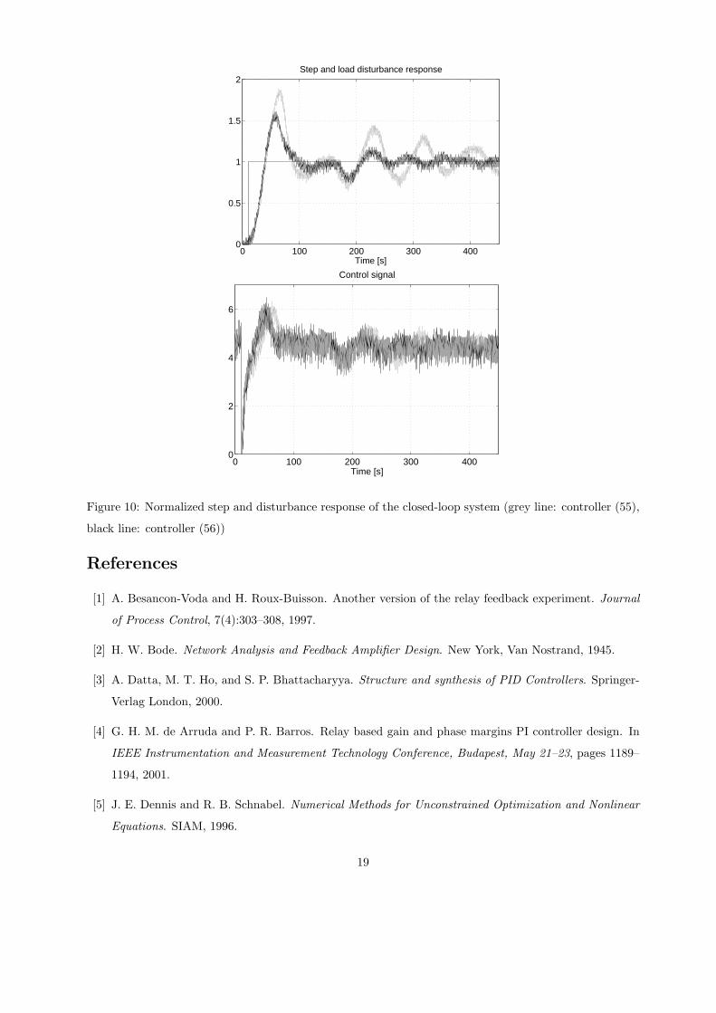
Now, consider that the operating point of the system is changed and, due to the system nonlinearity,
the closed-loop performance deteriorates. Consequently, the same controller at the new operating point
does not meet the specification (a phase margin Φm of = 55◦ and a crossover frequency ωm of 0.066 rad/s
are obtained) and the controller should be retuned. After one iteration, using the proposed tuning method,
the following controller is obtained:
K(s) = 23 (1 +1
42.3s+ 10.6s) (56)
The closed-loop system with this controller gives the following performance which is very close to the
desired one:
Φm = 73.7◦ ωm = 0.0791rad/s
A comparison of the normalized step response and disturbance response of the closed-loop system with
the two controllers is shown in Fig. 10. The effectiveness and rapidity of the proposed algorithm is shown
in Fig. 11 for an autotuning experiment. During the first 500 seconds the initial controller is implemented
on the real system and measurements are performed. Then the controller is updated and a new test is
carried out for measuring the phase margin as well as the crossover frequency.
As shown in this section, the proposed iterative tuning algorithm is fast enough to be used for the
autotuning of real processes, and is particularly appropriate for readjusting the controller parameters of
systems whose operating point changes slowly.
17
0 100 200 300 4000
0.5
1
1.5
2
Time [s]
Step and load disturbance response
0 100 200 300 4000
2
4
6
8Control signal
Time [s]
Figure 9: Normalized step and disturbance response of the closed-loop system (grey line: Kappa-Tau,
black line: proposed)
6 Conclusions
The derivatives of phase and amplitude of minimum-phase and stable plant models with respect to the
frequency have been approximated using the Bode’s integrals. The precision of the approximation for
typical industrial plant models is adequate for PID controller tuning. An iterative approach for tuning
the PID controller parameters with specifications on gain margin, phase margin and crossover frequency
was proposed. This approach takes advantage of Bode’s integrals to estimate the gradient and the Hessian
of a frequency criterion and therefore requires no parametric model of the plant. The proposed iterative
approach converges in a few iterations to the minimum of the frequency criterion and can be used for
autotuning of industrial plants.
18
0 100 200 300 4000
0.5
1
1.5
2
Time [s]
Step and load disturbance response
0 100 200 300 4000
2
4
6
Time [s]
Control signal
Figure 10: Normalized step and disturbance response of the closed-loop system (grey line: controller (55),
black line: controller (56))
References
[1] A. Besancon-Voda and H. Roux-Buisson. Another version of the relay feedback experiment. Journal
of Process Control, 7(4):303–308, 1997.
[2] H. W. Bode. Network Analysis and Feedback Amplifier Design. New York, Van Nostrand, 1945.
[3] A. Datta, M. T. Ho, and S. P. Bhattacharyya. Structure and synthesis of PID Controllers. Springer-
Verlag London, 2000.
[4] G. H. M. de Arruda and P. R. Barros. Relay based gain and phase margins PI controller design. In
IEEE Instrumentation and Measurement Technology Conference, Budapest, May 21–23, pages 1189–
1194, 2001.
[5] J. E. Dennis and R. B. Schnabel. Numerical Methods for Unconstrained Optimization and Nonlinear
Equations. SIAM, 1996.
19

0 200 400 600 800 1000-0.04
-0.02
0
0.02
0.04
Time [s]
Figure 11: Autotuning experiment (dashed: generated reference signal of the closed-loop system, solid:
output of the closed-loop system)
[6] W. K. Ho, C. C. Hang, and L. S. Cao. Tuning of PID controllers based on gain and phase margin
specifications. Automatica, 31(3):497–502, 1995.
[7] K. J. Astrom and T. Hagglund. Automatic tuning of simple regulators with specifications on phase
and amplitude margins. Automatica, 20(5):645–651, 1984.
[8] K. J. Astrom and T. Hagglund. PID Controllers: Theory, Design and Tuning. Instrument Society of
America, 2nd edition, 1995.
[9] B. Kristiansson, B. Lennartson, and C. M. Fransson. From PI to H∞ control in a unified framework.
In 39th IEEE-CDC, Sydney, Australia, pages 2740–2745, 2000.
[10] A. Leva. PID autotuning algorithm based on relay feedback. IEE Proceedings-D, 140(5):328–338,
September 1993.
[11] R. Longchamp and Y. Piguet. Closed-loop estimation of robustness margins by the relay method.
IEEE ACC, pages 2687–2691, 1995.
[12] Q. G. Wang, H. W. Fung, and Y. Zhang. PID tuning with exact gain and phase margins. ISA
Transactions, (38):243–249, 1999.
[13] Q. G. Wang, T. H. Lee, H. W. Fung, Q. Bi, and Y. Zhang. PID tuning for improved performance.
IEEE Transactions on CST, 7(4):3984–3989, 1999.
[14] M. Saeki. A new adaptive identification method of critical loop gain for multi-input multi-output
plants. 37th IEEE CDC, 4:3984–3989, 1998.
[15] T. S. Schei. Closed-loop tuning of PID controllers. In ACC, FA12, pages 2971–2975, 1992.
[16] C. C. Yu. Autotuning of PID Controllers: Relay Feedback Approach. Springer-Verlag London, 1999.
20