piecewise log-normal approximation of size distributions

HAL Id: hal-00295888https://hal.archives-ouvertes.fr/hal-00295888

Submitted on 27 Apr 2006

HAL is a multi-disciplinary open accessarchive for the deposit and dissemination of sci-entific research documents, whether they are pub-lished or not. The documents may come fromteaching and research institutions in France orabroad, or from public or private research centers.

L’archive ouverte pluridisciplinaire HAL, estdestinée au dépôt et à la diffusion de documentsscientifiques de niveau recherche, publiés ou non,émanant des établissements d’enseignement et derecherche français ou étrangers, des laboratoirespublics ou privés.

Piecewise log-normal approximation of size distributionsfor aerosol modelling

K. von Salzen

To cite this version:K. von Salzen. Piecewise log-normal approximation of size distributions for aerosol modelling. At-mospheric Chemistry and Physics, European Geosciences Union, 2006, 6 (5), pp.1351-1372. �hal-00295888�

https://hal.archives-ouvertes.fr/hal-00295888

https://hal.archives-ouvertes.fr

Atmos. Chem. Phys., 6, 1351–1372, 2006www.atmos-chem-phys.net/6/1351/2006/© Author(s) 2006. This work is licensedunder a Creative Commons License.

AtmosphericChemistry

and Physics

Piecewise log-normal approximation of size distributions for aerosolmodelling

K. von Salzen

Canadian Centre for Climate Modelling and Analysis, Science and Technology Branch, Environment Canada, Victoria,British Columbia, Canada

Received: 7 April 2005 – Published in Atmos. Chem. Phys. Discuss.: 14 June 2005Revised: 14 December 2005 – Accepted: 21 February 2006 – Published: 27 April 2006

Abstract. An efficient and accurate method for the represen-tation of particle size distributions in atmospheric models isproposed. The method can be applied, but is not necessar-ily restricted, to aerosol mass and number size distributions.A piecewise log-normal approximation of the number sizedistribution within sections of the particle size spectrum isused. Two of the free parameters of the log-normal approx-imation are obtained from the integrated number and massconcentration in each section. The remaining free parameteris prescribed. The method is efficient in a sense that only rel-atively few calculations are required for applications of themethod in atmospheric models.

Applications of the method in simulations of particlegrowth by condensation and simulations with a single col-umn model for nucleation, condensation, gravitational set-tling, wet deposition, and mixing are described. The resultsare compared to results from simulations employing single-and double-moment bin methods that are frequently used inaerosol modelling. According to these comparisons, the ac-curacy of the method is noticeably higher than the accuracyof the other methods.

1 Introduction

Models such as atmospheric general circulation models(AGCMs) and air quality models often lack the ability topredict aerosol size distributions mainly because of the largecomputational costs that are associated with a prognostictreatment of aerosol dynamical processes. Instead, param-eterizations of aerosol chemical and physical processes arecommonly based on highly idealized size distributions, forexample, with constant size parameters. However, aerosolsize distributions are considerably variable over a wide range

Correspondence to:K. von Salzen([email protected])

of spatial and temporal scales in the atmosphere (Gillianiet al., 1995; von Salzen et al., 2000; Birmili et al., 2001). Un-accounted variability in size distributions is a primary sourceof uncertainty in studies of aerosol effects on clouds and cli-mate (e.g.Feingold, 2003).

Consequently, accurate and computationally efficient nu-merical methods are required for the representation ofaerosol size distributions in aerosol models.

Observed aerosol number size distributions can often bewell approximated by a series of overlapping modes, withthe size distribution for each mode represented by the log-normal distribution, i.e.,

n(Rp) =dN

d ln(Rp/R0

)=

N√

2π ln σexp

{−

[ln(Rp/R0

)− ln

(Rg/R0

)]22 ln2 σ

},

with particle radiusRp, mode mean particle radiusRg, totalnumber of particles per unit volume (or mass)N , and geo-metric standard deviationσ (e.g.Whitby, 1978; Seinfeld andPandis, 1998; Remer et al., 1999). R0 is an arbitrary refer-ence radius (e.g. 1µm) that is required for a dimensionallycorrect formulation.

The so-called modal approach in aerosol modelling isbased on the idea that aerosol size distributions can be ap-proximated using statistical moments with idealized prop-erties (Whitby, 1981, 1997; Binkowski and Shankar, 1995;Wilck and Stratmann, 1997; Ackermann et al., 1998; Har-rington and Kreidenweis, 1998; Wilson et al., 2001). Typ-ically, a number of overlapping log-normally distributedmodes (e.g. for nucleation, accumulation and coarse mode)are assumed to account for different types of aerosols andprocesses in the atmosphere. An important variant ofthe modal approach is the quadrature method of moments,QMOM (McGraw, 1997; Wright et al., 2001; Yu et al.,

Published by Copernicus GmbH on behalf of the European Geosciences Union.

1352 K. von Salzen: Piecewise log-normal approximation

2003), which is not necessarily constrained to log-normallydistributed modes.

In practice, the log-normal distribution often yields goodapproximations of size distributions with clearly distinctmodes under ideal conditions. However, it has been rec-ognized that transport and non-linear dynamical processes,such as aerosol activation, condensation, and chemical pro-duction can lead to substantially skewed or even discontin-uous size distributions (e.g.Kerminen and Wexler, 1995;Gilliani et al., 1995; von Salzen and Schlunzen, 1999b;Zhang et al., 2002). Skewed size distributions are often re-lated to cloud processes so that an incomplete accounting ofskewness in aerosol size distributions is a substantial concernfor studies of the indirect effects of aerosols on climate.

Size distributions with non-ideal features can be well ap-proximated with the bin approach, also often called “sec-tional” or “discrete” approach (Gelbard and Seinfeld, 1980;Warren and Seinfeld, 1985; Gelbard, 1990; Seigneur, 1982;Jacobson, 1997; Lurmann et al., 1997; Russell and Seinfeld,1998; Meng et al., 1998; von Salzen and Schlunzen, 1999a;Pilinis et al., 2000; Gong et al., 2003). According to the binapproach, a range of particle sizes is subdivided into a num-ber of bins, or sections, with discrete values of the size dis-tribution in each bin.

It can be generally distinguished between single- andmulti-moment bin schemes, depending on the number of sta-tistical moments of the size distribution that are predicted.

In its original form with size-independent sub-bin parti-cle size distributions (e.g.Gelbard and Seinfeld, 1980), thesingle-moment approach is subject to significant numericaldiffusion when applied to simulations of aerosol dynamicalprocesses (e.g.Seigneur et al., 1986). However, an even moresubstantial disadvantage of the method is that the applicationof the method to the continuity equation for a single moment(e.g. particle mass) is not sufficient to ensure conservationof other moments (e.g. particle number). Other moments ofthe size distribution can be obtained from diagnostic relation-ships that are based on the predicted mass size distribution.Owing to the lack of a prognostic treatment, the diagnosedquantities can violate fundamental mathematical constraints,such as inequality relations and positive definiteness (Feller,1971). These can be significant problems if an insufficientnumber of bins is used. Despite these limitations, single-moment schemes are still widely used in aerosol models.

Numerous multi-moment schemes have been suggested asimprovements of the basic single-moment bin approach. Forexample,Tzivion et al. (1987) used bin-integrated aerosolnumber and mass concentrations to obtain sub-bin aerosolnumber and size distributions as linear functions of particlemass. In another example,Jacobson(1997) assigned the bin-integrated aerosol number and mass concentrations to a sin-gle particle size in each bin. According to this approach, pa-rameterizations of aerosol dynamical processes are appliedto the single-particle representation of the size distributionin each bin. Transfer of particles between different bins is

accomplished by combining particles with different sizes toproduce a new distribution for a single particle size in eachbin.

Several studies compared results of the modal and bin ap-proaches based on a limited number of simulations of aerosoldynamical processes (e.g.Seigneur et al., 1986; Zhang et al.,1999, 2002; Wilson et al., 2001; Korhonen et al., 2003). Ac-cording to the studies, the modal approach performed well interms of computationally efficiency and is able to reproduceimportant features of the size distributions. However, resultswith this approach were noticeably biased in simulations ofcoagulation and condensational growth in some of the stud-ies. On the other hand, the bin approach produced acceptableresults for a relatively large number of bins. Computationalefficiencies were generally lower for this approach in com-parison to the modal approach.

Both approaches have certain constraints that are problem-atic for the development of parameterizations in models.

For the bin method, the need to use a relatively largenumber of bins for sufficiently accurate solutions potentiallyleads to considerable computational costs. For example, sim-ulations of advection and horizontal diffusion cause an over-head of about 4% in CPU time for each additional prognostictracer in the current operational version of the Canadian Cen-tre for Climate Modelling and Analysis (CCCma) AGCM3(McFarlane et al., 2006). Parameterizations of aerosol dy-namical processes may lead to further and disproportionalincreases in CPU time.

A disadvantage for application of the modal approach ingeneral atmospheric models is the need to account for vary-ing degrees of overlap between different modes. As alreadypointed out, transport and aerosol dynamical processes oftenlead to changes in overlap and shape of modes. Relativelycomplicated treatments of aerosol dynamical processes havebeen proposed to allow distinct modes to merge into a singlemode, for example (e.g.Harrington and Kreidenweis, 1998;Whitby et al., 2002).

It is argued here that certain advantages offered by themodal approach (e.g. observed aerosols are often nearly log-normally distributed in parts of the size spectrum) and thesingle-moment bin approach (e.g. flexibility and simplicity)can be exploited for the development of a hybrid method withconsiderably improved performance.

The mathematical framework of a new method that isbased on a combination of the bin and the modal approachis described in Sect.2. An application of the method to ob-served size distributions and in simulations with a single col-umn model of the atmosphere are described in Sects.3 and5.

Atmos. Chem. Phys., 6, 1351–1372, 2006 www.atmos-chem-phys.net/6/1351/2006/

K. von Salzen: Piecewise log-normal approximation 1353

2 Formulation of the approximation method

2.1 Approximation of the aerosol number distribution

Without any loss of generality, an approximation of anaerosol number distribution may be expressed as a series oforthogonal functions, i.e.,

n(ϕ) =

∑i

ni(ϕ) , (1)

for the dimensionless size parameterϕ≡ ln(Rp/R0).The following set of functions in Eq. (1) is proposed:

ni(ϕ) = n0,i exp[−ψi

(ϕ − ϕ0,i

)2]H(ϕ − ϕi−1/2

)H(ϕi+1/2 − ϕ

), (2)

wheren0,i , ψi , andϕ0,i are fitting parameters that determinethe magnitude, width, respectively mean of the distribution(Sect.2.2). H(x) denotes the Heaviside step function, i.e.

H(x) =

0 if x < 0 ,12 if x = 0 ,

1 if x > 0 .

so thatni=0 outside each sectioni with the size rangeϕi−1/2≤ϕ≤ϕi+1/2. Log-normal distributions with varyingproperties between sections are used as basis functions ineach section (Eq.2). Hence, Eqs. (1) and (2) define a piece-wise log-normal approximation (PLA) of the aerosol numberdistribution.

As will be demonstrated in the following sections, Eqs. (1)and (2) can be directly used for the approximation of ob-served size distributions and development of parameteriza-tions in models.

Note that similar to the single-moment bin approach (e.g.,which can be obtained forψi=0), the approach in Eq. (2)ensures thatn (ϕ)≥0 for any given value ofϕ. This is notnecessarily the case for other potential prescriptions, e.g. arepresentation of the basis functions in terms of polynomials.Additionally, the PLA method presented here has the advan-tages that the method is exact for strictly log-normally dis-tributed aerosol number concentrations and that it is straight-forward to calculate any higher moment of the approximatedsize distribution. The latter is particularly important forpotential applications of the method to the development ofparameterizations. Finally, approximated size distributionsgenerally converge to the exact solution for a sufficientlylarge number of sections for appropriate choices of the fit-ting parameters.

2.2 Determination of the fitting parameters

The fitting parametersn0,i , ψi , andϕ0,i in Eq. (2) can be ob-tained in various ways. Here it is proposed to prescribe oneof these parameters and to calculate the other two parameters

for given integrated number (Ni) and mass (Mi) concentra-tions in each section. This approach leads to a self-consistentrepresentation of these quantities in numerical models andalso leads to expressions that are relatively straightforwardto evaluate.

First, it is useful to introduce thekth momentµki of thesize distribution in sectioni, i.e.

µki ≡

∫ ϕi+1/2

ϕi−1/2

Rkpn (ϕ) dϕ .

Using Eqs. (1) and (2) it follows that

µki = Rk0 n0,i Iki ,

with

Iki =1

2

√π

|ψi |fki exp

(kϕ0,i +

k2

4|ψi |

),

and

fki =

{erf(aki+1/2

)− erf

(aki−1/2

)if ψi > 0 ,

erfi(aki+1/2

)− erfi

(aki−1/2

)if ψi < 0 .

The arguments of the error function erf(x) and imaginary er-ror function erfi(x) in fki are given by:

aki+1/2 = −√

|ψi | (1ϕi −1ϕ?)−k sgn(ψi)

2√

|ψi |,

aki−1/2 = −√

|ψi |1ϕi −k sgn(ψi)

2√

|ψi |,

with sgn(x)=2H(x)−1,

1ϕi ≡ ϕ0,i − ϕi−1/2 , (3)

and section size1ϕ?≡ϕi+1/2−ϕi−1/2.Consequently, the integrated number (k=0) and mass

(k=3) concentrations in each section are:

Ni = n0,i I0i , (4)

Mi =4π

3ρp,iR

30 n0,i I3i , (5)

whereρp,i is the particle density,As shall be seen, it is useful for the calculation of the fitting

parameters to also introduce the dimensionless size ratio

ri ≡ϕi − ϕi−1/2

1ϕ?, (6)

where

ϕi ≡ ln

[1

R0

(3

4πρp,i

Mi

Ni

)1/3].

is an effective particle size.ri (Eq.6) characterizes the skewness of the approximated

size distribution within each section. For example, considertwo populations of aerosol particles that have the same total

www.atmos-chem-phys.net/6/1351/2006/ Atmos. Chem. Phys., 6, 1351–1372, 2006



for minimum and maximum particle sizes in the given sizerange (i.e. corresponding to the section boundaries).

Combination of an expression forMi/Ni from Eqs. (4)and (5) with Eq. (6) conveniently eliminatesn0,i, i.e.

f3i

f0i= exp

[

3 (ri∆ϕ⋆ −∆ϕi)−9

4|ψi|

]

. (7)

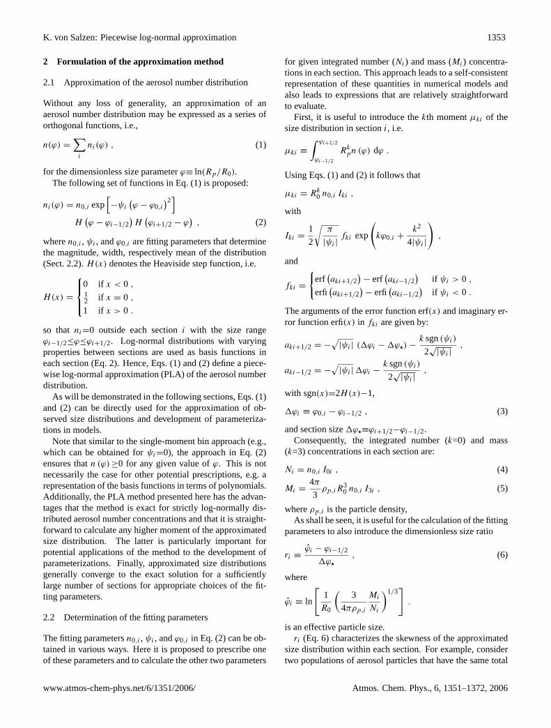
The only unknown parameters in this equation are∆ϕi andψi if Ni andMi and the section boundaries are given. It issuggested to prescribeψi so that this equation can be used todetermine∆ϕi. Subsequently, Eq. (3) can be used to deter-mine the value of the fitting parameterϕ0,i.

An example for∆ϕi from the solution of Eq. (7) is shownin Fig. 1 for a section size∆ϕ⋆ = 1

3 [ln(1.75) − ln(0.05)](i.e. similar to the application in Section 3). Note that Eq.(7)

r i

ψi

Fig. 1. ∆ϕi [Eq. (3)] according to Eq. (7). No solution exists in theshaded area.

does not have any solution for∆ϕi within a certain range ofvalues ofψi andri. Therefore,ψi is selected such thatψi isequal to an arbitrarily prescribed valueψm,i inside the regionfor which a solution of Eq. (7) exists. Outside that region, adifferent value than that is selected in order to ensure thatasolution exists. In that case,ψi should be as close as possibleto ψm,i. Therefore,

ψi =

{

min (ψm,i, ψl) if ψm,i < 0 ,

max (ψm,i, ψl) if ψm,i > 0 ,(8)

where ψl represents a threshold for which a solution ofEq. (7) can be found (i.e. as indicated by the green line inFig. 1). This algorithm can be applied to0 ≤ ri ≤ 1 and−∞ ≤ ψm,i ≤ ∞ for

limri→0,1

ψl =

{

+∞ if ψi > 0 ,

−∞ if ψi < 0 .

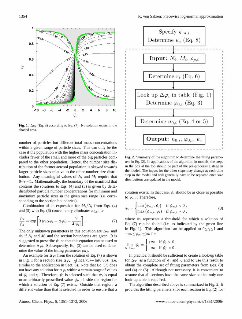
In practice, it should be sufficient to create a look-up tablefor ∆ϕi as a function ofψi andri and to use this result toobtain the complete set of fitting parameters from Eqs. (3)and (4) or (5). Although not necessary, it is convenient toassume that all sections have the same size so that only onelook-up table is required.

The algorithm described above is summarized in Fig. 2. Itprovides the fitting parameters for each section in Eq. (2) forgiven values of the number and mass concentrations in thesame section.

Specifyψm,i

Determineψi [Eq. (8)]

?

Input: Ni,Mi, ρp,i

?

Determineri [Eq. (6)]

?

Look up∆ϕi in table (Fig. 1)

Determineϕ0,i [Eq. (3)]

?

Determinen0,i [Eq. (4) or (5)]

?

Output: n0,i, ϕ0,i, ψi

Fig. 2. Summary of the algorithm to determine the fitting parame-ters in Eq. (2). In applications of the algorithm in models, the stepsin the box at the top should be part of the pre-processing stage inthe model. The inputs for the other steps may change at each timestep in the model and will generally have to be repeated once sizedistributions are updated in the model.

While the accuracy of the approximation of a size distri-bution in terms of log-normal size distributions accordingtoEq. (2) depends on the values ofψm,i, no attempt is madehere to calculateψm,i as part of the algorithm. Tests withthe method under various conditions give evidence for a rel-atively weak dependency of the errors of the method onψm,i

within a substantial range for this parameter (e.g., Sections 3and 5).

The accuracy of the transformations fromNi and Mi

to log-normal size distributions according to the algorithm(Fig. 2) and vice versa [Eqs. (4) and (5)] depends on the ac-curacy of the tabulated data for∆ϕi. However, for typicalapplications, (e.g. in the examples presented in the followingsections) sufficient accuracy can usually be achieved for rea-sonably small table sizes. If necessary, the accuracy can beadditionally increased by directly solving Eq. (7) insteadof(or in addition to) the table look-up step.

It should be noted here that similar to the approach pro-posed here, Zender et al. (2003) proposed a piecewise-

Fig. 1. 1ϕi (Eq. 3) according to Eq. (7). No solution exists in theshaded area.

number of particles but different total mass concentrationswithin a given range of particle sizes. This can only be thecase if the population with the higher mass concentration in-cludes fewer of the small and more of the big particles com-pared to the other population. Hence, the number size dis-tribution of the former aerosol population is skewed towardslarger particle sizes relative to the other number size distri-bution. Any meaningful values ofNi andMi require that0≤ri≤1. Mathematically, the boundary of the manifold thatcontains the solutions to Eqs. (4) and (5) is given by delta-distributed particle number concentrations for minimum andmaximum particle sizes in the given size range (i.e. corre-sponding to the section boundaries).

Combination of an expression forMi/Ni from Eqs. (4)and (5) with Eq. (6) conveniently eliminatesn0,i , i.e.

f3i

f0i= exp

[3(ri1ϕ? −1ϕi)−

9

4|ψi |

]. (7)

The only unknown parameters in this equation are1ϕi andψi if Ni andMi and the section boundaries are given. It issuggested to prescribeψi so that this equation can be used todetermine1ϕi . Subsequently, Eq. (3) can be used to deter-mine the value of the fitting parameterϕ0,i .

An example for1ϕi from the solution of Eq. (7) is shownin Fig. 1 for a section size1ϕ?=1

3[ln(1.75)− ln(0.05)] (i.e.similar to the application in Sect.3). Note that Eq. (7) doesnot have any solution for1ϕi within a certain range of valuesof ψi andri . Therefore,ψi is selected such thatψi is equalto an arbitrarily prescribed valueψm,i inside the region forwhich a solution of Eq. (7) exists. Outside that region, adifferent value than that is selected in order to ensure that a

Specify ψm,i

Determine ψi (Eq. 8)

?

Input: Ni, Mi, ρp,i

?

Determine ri (Eq. 6)

?

Look up ∆ϕi in table (Fig. 1)

Determine ϕ0,i (Eq. 3)

?

Determine n0,i (Eq. 4 or 5)

?

Output: n0,i, ϕ0,i, ψi

Fig. 2. Summary of the algorithm to determine the fitting parame-ters in Eq. (2). In applications of the algorithm in models, the stepsin the box at the top should be part of the pre-processing stage inthe model. The inputs for the other steps may change at each timestep in the model and will generally have to be repeated once sizedistributions are updated in the model.

solution exists. In that case,ψi should be as close as possibletoψm,i . Therefore,

ψi =

{min

(ψm,i, ψl

)if ψm,i < 0 ,

max(ψm,i, ψl

)if ψm,i > 0 ,

(8)

whereψl represents a threshold for which a solution ofEq. (7) can be found (i.e. as indicated by the green linein Fig. 1). This algorithm can be applied to 0≤ri≤1 and−∞≤ψm,i≤∞ for

limri→0,1

ψl =

{+∞ if ψi > 0 ,

−∞ if ψi < 0 .

In practice, it should be sufficient to create a look-up tablefor 1ϕi as a function ofψi andri and to use this result toobtain the complete set of fitting parameters from Eqs. (3)and (4) or (5). Although not necessary, it is convenient toassume that all sections have the same size so that only onelook-up table is required.

The algorithm described above is summarized in Fig.2. Itprovides the fitting parameters for each section in Eq. (2) for



given values of the number and mass concentrations in thesame section.

While the accuracy of the approximation of a size distri-bution in terms of log-normal size distributions according toEq. (2) depends on the values ofψm,i , no attempt is madehere to calculateψm,i as part of the algorithm. Tests withthe method under various conditions give evidence for a rel-atively weak dependency of the errors of the method onψm,iwithin a substantial range for this parameter (e.g., Sects.3and5).

The accuracy of the transformations fromNi and Mi

to log-normal size distributions according to the algorithm(Fig. 2) and vice versa (Eqs.4 and 5) depends on the ac-curacy of the tabulated data for1ϕi . However, for typicalapplications, (e.g. in the examples presented in the followingsections) sufficient accuracy can usually be achieved for rea-sonably small table sizes. If necessary, the accuracy can beadditionally increased by directly solving Eq. (7) instead of(or in addition to) the table look-up step.

It should be noted here that similar to the approach pro-posed here,Zender et al.(2003) proposed a piecewise-analytical representation of the aerosol size distribution.Specifically, they assumed that the aerosol mass is log-normally distributed in each section. However, their ap-proach is quite similar to the single-moment sectional ap-proach. In particular, the assumption of time-invariant sizedistributions within each section, with the mass being theonly predicted variable, clearly distinguishes their approachfrom the PLA method. Consequently, aerosol number (orany other moment) will generally not be conserved in sim-ulations with Zender et al.’s approach. Additionally, the as-sumption of a time-invariant size distribution could be quiteproblematic at small to moderate numbers of sections. Forexample, this assumption cannot be expected to not workwell for gravitational settling of mineral dust particles whichtypically causes large variations in the particle size distribu-tion with height. In contrast to Zender et al.’s approach, thePLA method can be used to account for changes in the sizedistribution at any given particle size scale.

2.3 Computational costs of the method

For applications of the PLA method in numerical models itis useful to consider the computational costs that are poten-tially associated with the method. In a model, the calcula-tions of ri andn0,i in Fig. 2 would likely be the most ex-pensive steps because of the need to evaluate the functionsln(x) and erf(x) [respectively erfi(x)] for each section ac-cording to Eqs. (6) and (4). In comparison, the costs associ-ated with the table look-up are relatively minor for a typicalFortran 90-implementation on an IBM pSeries 390 systemwith POWER4 microprocessor architecture at the CanadianMeteorological Centre (i.e.≈1/3 of the total costs of themethod). These costs are considerably smaller than the costs

that would typically be associated with parameterizations ofbulk aerosol processes in atmospheric models.

3 Application to observed size distributions

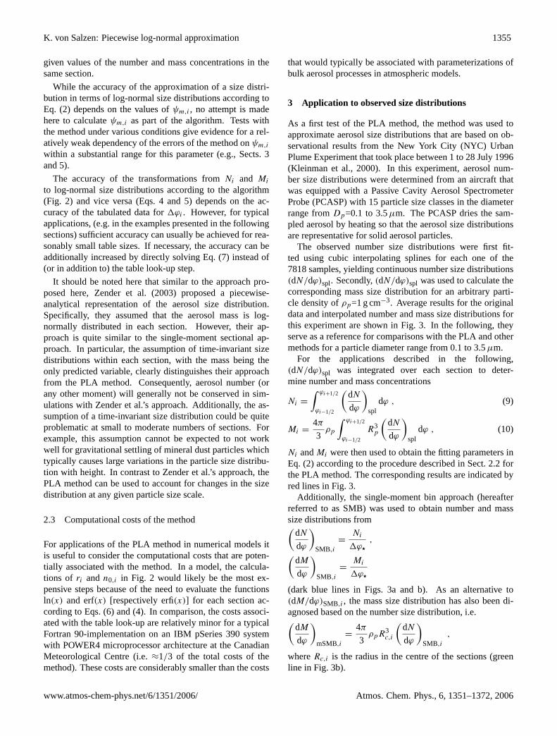
As a first test of the PLA method, the method was used toapproximate aerosol size distributions that are based on ob-servational results from the New York City (NYC) UrbanPlume Experiment that took place between 1 to 28 July 1996(Kleinman et al., 2000). In this experiment, aerosol num-ber size distributions were determined from an aircraft thatwas equipped with a Passive Cavity Aerosol SpectrometerProbe (PCASP) with 15 particle size classes in the diameterrange fromDp=0.1 to 3.5µm. The PCASP dries the sam-pled aerosol by heating so that the aerosol size distributionsare representative for solid aerosol particles.

The observed number size distributions were first fit-ted using cubic interpolating splines for each one of the7818 samples, yielding continuous number size distributions(dN/dϕ)spl. Secondly,(dN/dϕ)spl was used to calculate thecorresponding mass size distribution for an arbitrary parti-cle density ofρp=1 g cm−3. Average results for the originaldata and interpolated number and mass size distributions forthis experiment are shown in Fig.3. In the following, theyserve as a reference for comparisons with the PLA and othermethods for a particle diameter range from 0.1 to 3.5µm.

For the applications described in the following,(dN/dϕ)spl was integrated over each section to deter-mine number and mass concentrations

Ni =

∫ ϕi+1/2

ϕi−1/2

(dN

dϕ

)spl

dϕ , (9)

Mi =4π

3ρp

∫ ϕi+1/2

ϕi−1/2

R3p

(dN

dϕ

)spl

dϕ , (10)

Ni andMi were then used to obtain the fitting parameters inEq. (2) according to the procedure described in Sect.2.2 forthe PLA method. The corresponding results are indicated byred lines in Fig.3.

Additionally, the single-moment bin approach (hereafterreferred to as SMB) was used to obtain number and masssize distributions from(

dN

dϕ

)SMB,i

=Ni

1ϕ?,(

dM

dϕ

)SMB,i

=Mi

1ϕ?

(dark blue lines in Figs.3a and b). As an alternative to(dM/dϕ)SMB,i , the mass size distribution has also been di-agnosed based on the number size distribution, i.e.(

dM

dϕ

)mSMB,i

=4π

3ρpR

3c,i

(dN

dϕ

)SMB,i

,

whereRc,i is the radius in the centre of the sections (greenline in Fig.3b).


1356 K. von Salzen: Piecewise log-normal approximation6 K. von Salzen: Piecewise log-normal approximation(a)

dN dln(R p=R 0)( m�3 )

Dp (�m)

(b)

Dp (�m)dM dln(R p=R 0)(�gm�3 )

Fig. 3. Average observed (dashed line) and interpolated size distributions (full black lines) for aerosol number (left column) and mass (rightcolumn) for all samples during the NYC Urban Plume Experiment. Red lines refer to the corresponding results of the PLA method for 3sections. Similar, dark blue lines in (a) and (b) refer to results of the single-moment bin (SMB) approach. The green linein (b) is for adiagnosed size distribution based on results of the bin method in (a) as described in the text.

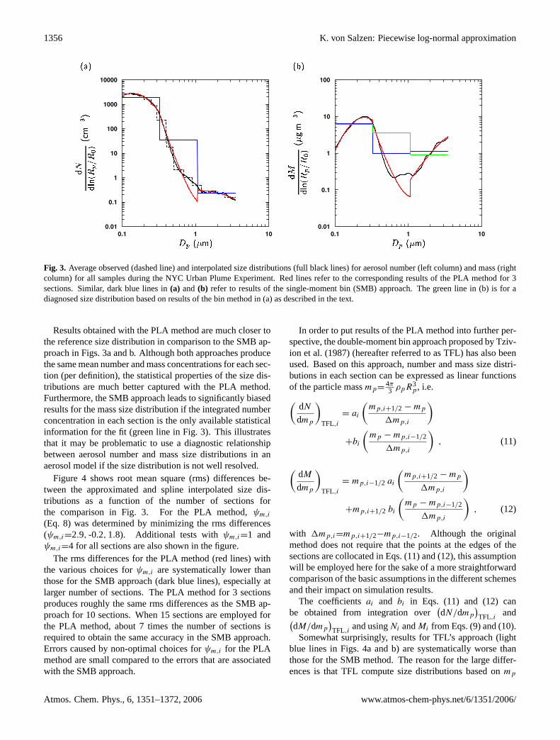
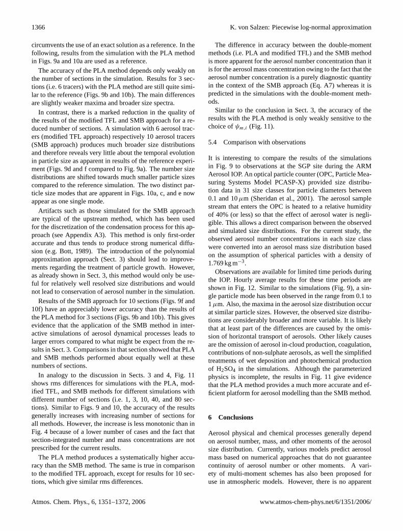
larger number of sections. The PLA method for 3 sectionsproduces roughly the same rms differences as the SMB ap-proach for 10 sections. When 15 sections are employed forthe PLA method, about 7 times the number of sections isrequired to obtain the same accuracy in the SMB approach.Errors caused by non-optimal choices forψm,i for the PLAmethod are small compared to the errors that are associatedwith the SMB approach.

In order to put results of the PLA method into further per-spective, the double-moment bin approach proposed by Tziv-ion et al. (1987) (hereafter referred to as TFL) has also beenused. Based on this approach, number and mass size distri-butions in each section can be expressed as linear functionsof the particle massmp = 4π

3 ρpR3p, i.e.

(

dN

dmp

)

TFL,i

= ai

(

mp,i+1/2 −mp

∆mp,i

)

+bi

(

mp −mp,i−1/2

∆mp,i

)

,

(11)

(

dM

dmp

)

TFL,i

= mp,i−1/2 ai

(

mp,i+1/2 −mp

∆mp,i

)

+mp,i+1/2 bi

(

mp −mp,i−1/2

∆mp,i

)

,

(12)

with ∆mp,i = mp,i+1/2 −mp,i−1/2. Although the originalmethod does not require that the points at the edges of thesections are collocated in Eqs. (11) and (12), this assumptionwill be employed here for the sake of a more straightforwardcomparison of the basic assumptions in the different schemesand their impact on simulation results.

The coefficientsai and bi in Eqs. (11) and (12) canbe obtained from integration over(dN/dmp)TFL,i and

(dM/dmp)TFL,i and usingNi andMi from Eqs. (9) and(10).

Somewhat surprisingly, results for TFL’s approach (lightblue lines in Fig. 4 a and b) are systematically worse thanthose for the SMB method. The reason for the large differ-ences is that TFL compute size distributions based onmp

rather than onϕ. This approach is problematic in the con-text of the observed size distributions from the NYC UrbanPlume Experiment because(dN/dmp)spl is much steeperthan(dN/dϕ)spl. It can be analytically shown that for anygiven linear number distributiondN/dmp, the piecewise-linear approximation ofdN/dmp according to TFL’s ap-proach systematically produces smaller absolute values forthe slopes of the distribution in each section.

The results for TFL’s approach demonstrate that it is im-portant to consider the same particle size variable when com-paring results for different approximation methods. For afairer comparison, TFL’s approach has been modified in or-der to express the approximated number and mass size dis-tributions as linear functions ofϕ instead, i.e.

(

dN

dϕ

)

mTFL,i

= am,i

(

ϕi+1/2 − ϕ

∆ϕ⋆

)

+bm,i

(

ϕ− ϕi−1/2

∆ϕ⋆

)

,

(13)

(

dM

dϕ

)

mTFL,i

= mp,i−1/2 am,i

(

ϕi+1/2 − ϕ

∆ϕ⋆

)

+mp,i+1/2 bm,i

(

ϕ− ϕi−1/2

∆ϕ⋆

)

,

(14)

where, in analogy to the original approach, coefficientsam,i

andbm,i can be obtained from integration.

Fig. 3. Average observed (dashed line) and interpolated size distributions (full black lines) for aerosol number (left column) and mass (rightcolumn) for all samples during the NYC Urban Plume Experiment. Red lines refer to the corresponding results of the PLA method for 3sections. Similar, dark blue lines in(a) and(b) refer to results of the single-moment bin (SMB) approach. The green line in (b) is for adiagnosed size distribution based on results of the bin method in (a) as described in the text.

Results obtained with the PLA method are much closer tothe reference size distribution in comparison to the SMB ap-proach in Figs.3a and b. Although both approaches producethe same mean number and mass concentrations for each sec-tion (per definition), the statistical properties of the size dis-tributions are much better captured with the PLA method.Furthermore, the SMB approach leads to significantly biasedresults for the mass size distribution if the integrated numberconcentration in each section is the only available statisticalinformation for the fit (green line in Fig.3). This illustratesthat it may be problematic to use a diagnostic relationshipbetween aerosol number and mass size distributions in anaerosol model if the size distribution is not well resolved.

Figure 4 shows root mean square (rms) differences be-tween the approximated and spline interpolated size dis-tributions as a function of the number of sections forthe comparison in Fig.3. For the PLA method,ψm,i(Eq. 8) was determined by minimizing the rms differences(ψm,i=2.9, -0.2,1.8). Additional tests withψm,i=1 andψm,i=4 for all sections are also shown in the figure.

The rms differences for the PLA method (red lines) withthe various choices forψm,i are systematically lower thanthose for the SMB approach (dark blue lines), especially atlarger number of sections. The PLA method for 3 sectionsproduces roughly the same rms differences as the SMB ap-proach for 10 sections. When 15 sections are employed forthe PLA method, about 7 times the number of sections isrequired to obtain the same accuracy in the SMB approach.Errors caused by non-optimal choices forψm,i for the PLAmethod are small compared to the errors that are associatedwith the SMB approach.

In order to put results of the PLA method into further per-spective, the double-moment bin approach proposed byTziv-ion et al.(1987) (hereafter referred to as TFL) has also beenused. Based on this approach, number and mass size distri-butions in each section can be expressed as linear functionsof the particle massmp=4π

3 ρpR3p, i.e.(

dN

dmp

)TFL,i

= ai

(mp,i+1/2 −mp

1mp,i

)+bi

(mp −mp,i−1/2

1mp,i

), (11)

(dM

dmp

)TFL,i

= mp,i−1/2 ai

(mp,i+1/2 −mp

1mp,i

)+mp,i+1/2 bi

(mp −mp,i−1/2

1mp,i

), (12)

with 1mp,i=mp,i+1/2−mp,i−1/2. Although the originalmethod does not require that the points at the edges of thesections are collocated in Eqs. (11) and (12), this assumptionwill be employed here for the sake of a more straightforwardcomparison of the basic assumptions in the different schemesand their impact on simulation results.

The coefficientsai and bi in Eqs. (11) and (12) canbe obtained from integration over

(dN/dmp

)TFL,i and(

dM/dmp)TFL,i and usingNi andMi from Eqs. (9) and (10).

Somewhat surprisingly, results for TFL’s approach (lightblue lines in Figs.4a and b) are systematically worse thanthose for the SMB method. The reason for the large differ-ences is that TFL compute size distributions based onmp


K. von Salzen: Piecewise log-normal approximation 1357K. von Salzen: Piecewise log-normal approximation 7

( )rmsdi�eren e( m�3 )

number of se tions

(d)

number of se tionsrmsdi�eren e(�gm�3 )

(a)rmsdi�eren e( m�3 )

number of se tions

(b)


Fig. 4. Mean rms differences between the approximated and spline interpolated size distributions for aerosol number (a and c) and mass (band d) for all samples from the NYC experiment. Dark blue lines refer to the single-moment bin approach and red lines to thePLA methodfor optimal choice ofψm,i (full line), ψm,i = 1 (long dashed line), andψm,i = 4 (short dashed line). In a and b, light blue lines referto the approach by Tzivion et al. (1987) and pink lines to the modified version of this approach. c and d show results for the polynomialapproximations based on the number (yellow lines) and mass (orange lines) size distributions. Only results for less than doubling of massbetween section boundaries are considered for the other methods because these methods are typically not employed for broader sections.

The modified version of this approach (pink lines) yieldssystematically better performance than the SMB approachaccording to Fig. 4 a and b. However, neither the originalnor the modified version of TFL’s approach outperform thePLA method at any given number of sections.

Finally, it is also interesting to compare the PLA methodwith a representation of the aerosol size distribution in termsof polynomials. For example, Dhaniyala and Wexler (1996)and von Salzen and Schlunzen (1999a) have used second-order polynomials to represent aerosol mass size distribu-tions following the approach that was originally proposedby Bott (1989). An interesting feature of Bott’s approach is

that it ensures conservation from renormalization of the fittedsize distribution. However, similar to other single-momentschemes, other moments of the size distribution can only beobtained from diagnostic relationships.

Fig. 4 c and d shows results from applications of the poly-nomial approach to the number (yellow lines) and mass (or-ange lines) size distributions from the NYC Urban Plume Ex-periment based on second-order polynomials. For simplicityand lack of a better approach, the corresponding mass (yel-low line in Fig. 4 d) and number (orange line in Fig. 4 c) sizedistributions have been diagnosed by scaling of the approx-imated size distributions withmp, respectively1/mp. Note

Fig. 4. Mean rms differences between the approximated and spline interpolated size distributions for aerosol number (a andc) and mass (bandd) for all samples from the NYC experiment. Dark blue lines refer to the single-moment bin approach and red lines to the PLA methodfor optimal choice ofψm,i (full line), ψm,i=1 (long dashed line), andψm,i=4 (short dashed line). In (a) and (b), light blue lines refer tothe approach byTzivion et al.(1987) and pink lines to the modified version of this approach. (c) and (d) show results for the polynomialapproximations based on the number (yellow lines) and mass (orange lines) size distributions. Only results for less than doubling of massbetween section boundaries are considered for the other methods because these methods are typically not employed for broader sections.

rather than onϕ. This approach is problematic in the con-text of the observed size distributions from the NYC UrbanPlume Experiment because

(dN/dmp

)spl is much steeper

than (dN/dϕ)spl. It can be analytically shown that for anygiven linear number distribution dN/dmp, the piecewise-linear approximation of dN/dmp according to TFL’s ap-proach systematically produces smaller absolute values forthe slopes of the distribution in each section.

The results for TFL’s approach demonstrate that it is im-portant to consider the same particle size variable when com-

paring results for different approximation methods. For afairer comparison, TFL’s approach has been modified in or-der to express the approximated number and mass size dis-tributions as linear functions ofϕ instead, i.e.

(dN

dϕ

)mTFL,i

= am,i

(ϕi+1/2 − ϕ

1ϕ?

)+bm,i

(ϕ − ϕi−1/2

1ϕ?

), (13)


1358 K. von Salzen: Piecewise log-normal approximation(dM

dϕ

)mTFL,i

= mp,i−1/2 am,i

(ϕi+1/2 − ϕ

1ϕ?

)+mp,i+1/2 bm,i

(ϕ − ϕi−1/2

1ϕ?

), (14)

where, in analogy to the original approach, coefficientsam,iandbm,i can be obtained from integration.

The modified version of this approach (pink lines) yieldssystematically better performance than the SMB approachaccording to Figs.4a and b. However, neither the originalnor the modified version of TFL’s approach outperform thePLA method at any given number of sections.

Finally, it is also interesting to compare the PLA methodwith a representation of the aerosol size distribution in termsof polynomials. For example,Dhaniyala and Wexler(1996)and von Salzen and Schlunzen(1999a) have used second-order polynomials to represent aerosol mass size distribu-tions following the approach that was originally proposedby Bott (1989). An interesting feature of Bott’s approach isthat it ensures conservation from renormalization of the fittedsize distribution. However, similar to other single-momentschemes, other moments of the size distribution can only beobtained from diagnostic relationships.

Figures4c and d show results from applications of thepolynomial approach to the number (yellow lines) and mass(orange lines) size distributions from the NYC Urban PlumeExperiment based on second-order polynomials. For sim-plicity and lack of a better approach, the corresponding mass(yellow line in Fig.4d) and number (orange line in Fig.4c)size distributions have been diagnosed by scaling of the ap-proximated size distributions withmp, respectively 1/mp.Note that this approach does not ensure conservation for thediagnosed quantities.

The polynomial approach gives very good results whenapplied to the observed size distributions for 20 or more sec-tions for both versions of this approach and the diagnosedquantities. However, the rms differences are considerable forthe diagnosed number size distribution at smaller number ofsections if the method is applied to the mass size distribution(and vice versa).

A more substantial problem with the polynomial approachis that it produced negative values of the size distribution forsome of the sections in the simulations. Although there aretechniques that can be used to prevent negative results in ap-plications of the method to tracer advection (Bott, 1989) andcoagulation (Bott, 1998), it does not seem straightforward tocome up with a general correction method.

Note that the polynomial approach will no longer be con-sidered in the following owing to the lack of a general correc-tion method for negative values which would be required forthe development of parameterizations for gravitational set-tling and other aerosol dynamical processes.

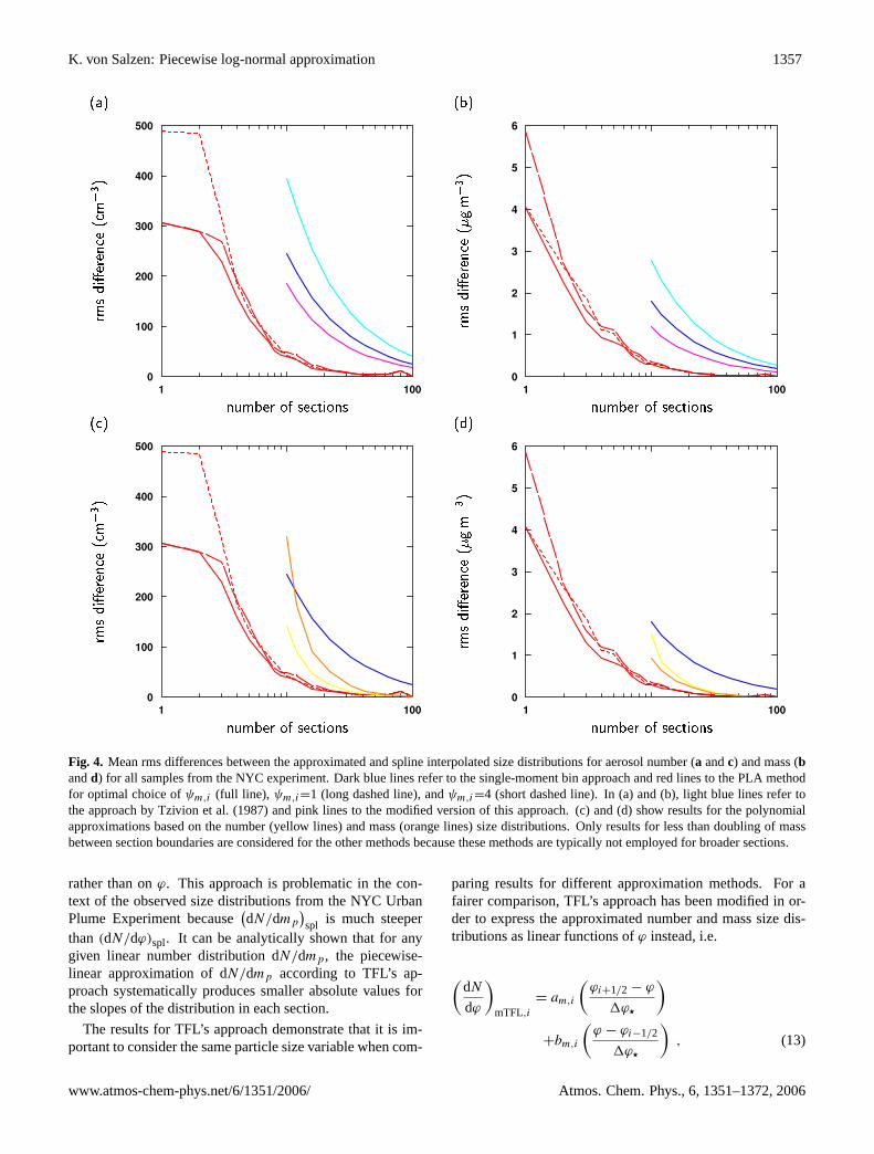
4 Application to particle growth by condensation

The results from the previous section give evidence that thePLA method can be used to accurately approximate atmo-spheric aerosol size distributions. However, a more impor-tant question from a practical point of view is whether themethod is also appropriate for modelling individual aerosoldynamical processes. Owing to the considerable number ofrelevant aerosol dynamical processes and the wide range ofatmospheric conditions that influence aerosols size distribu-tions in the atmosphere, an impractically large number oftests would be required to address this question in a suffi-ciently general way. A detailed study on the performanceof the scheme in the context of different aerosol dynamicalprocesses is outside the scope of this paper. Instead, a sin-gle application of the method to the simulation of particlegrowth by condensation is discussed in the following. Sev-eral other authors have studied solutions of the condensationequation in the past to test the performance of different nu-merical schemes. The advantage of this approach is that rel-atively simple analytical solutions of the condensation equa-tion are available for comparisons with numerical solutionsunder certain idealized circumstances.

A simple analytical solution of the condensation equationunder the assumption of continuum regime growth, unity ac-commodation coefficient, and constant gas-phase supersatu-ration was presented bySeinfeld and Pandis(1998). Underthese assumptions, the time evolution of the aerosol particlediameter is given by

dDpdt

=Ag

Dp, (15)

with

Ag =

(4DC

ρp

),

the concentrationC of the gas (in kg m−3), and its diffusivityD (in m2 s−1).

Application of Eq. (15) to an initial size distribution,

dN

dϕ(t = 0) = Dp

N0√

2π ln σexp

[−

ln2 (Dp/Dpg)2 ln2 σ

],

for constantN0, σ , andDpg yields the solution

dN

dϕ(t) =

D2p(

D2p − 2Agt

) 12

N√

2π ln σ

exp

−

ln2[(D2p − 2Agt

) 12/Dpg

]2 ln2 σ

. (16)

Results for Eq. (16) are shown in Fig.5 for the case thatwas studied bySeinfeld and Pandis(1998)(black lines).


K. von Salzen: Piecewise log-normal approximation 1359K. von Salzen: Piecewise log-normal approximation 9(a)dN dln(R p=R 0)( m�3 )

Dp (�m)

(b) ( )

Fig. 5. Size distributions for analytical and numerical solutionsof the condensation equation at timest = 0 (a),t = 2 min (b), andt = 10 min(c). Results are shown for the analytical solution (black),PLA (red), SMB (blue), and modified TFL (pink) methods, forC = 4.09µg m−3

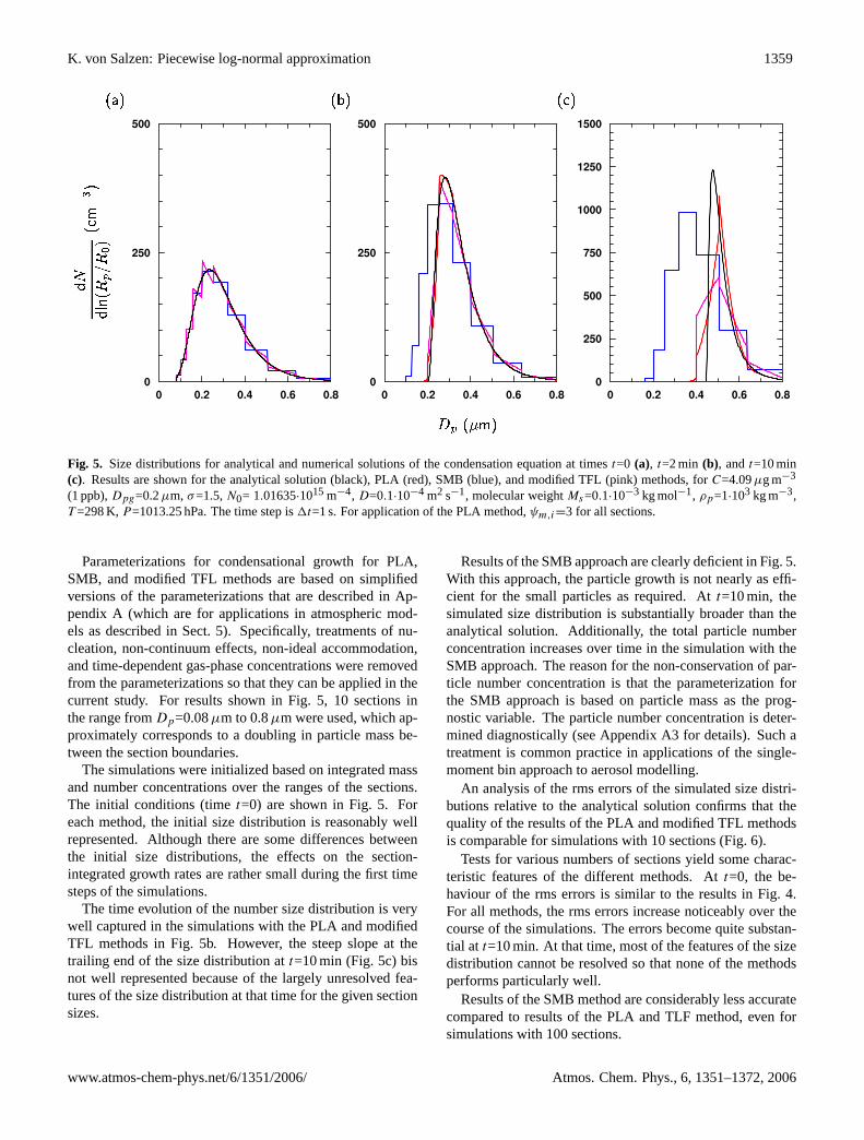
(1 ppb),Dpg = 0.2µm, σ = 1.5,N0 = 1.01635 · 1015 m−4, D = 0.1 · 10−4 m2 s−1, molecular weightMs = 0.1 · 10−3 kg mol−1, ρp =1 · 103 kg m−3, T = 298 K,P = 1013.25 hPa. The time step is∆t = 1 s. For application of the PLA method,ψm,i = 3 for all sections.

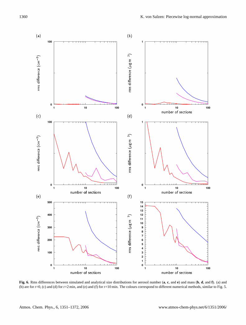
An analysis of the rms errors of the simulated size distri-butions relative to the analytical solution confirms that thequality of the results of the PLA and modified TFL methodsis comparable for simulations with 10 sections (Fig. 6).

Tests for various numbers of sections yield some charac-teristic features of the different methods. Att = 0, the be-haviour of the rms errors is similar to the results in Fig. 4.For all methods, the rms errors increase noticeably over thecourse of the simulations. The errors become quite substan-tial att = 10 min. At that time, most of the features of the sizedistribution cannot be resolved so that none of the methodsperforms particularly well.

Results of the SMB method are considerably less accuratecompared to results of the PLA and TLF method, even forsimulations with 100 sections.

At t = 1 min, the PLA method produces noticeably lowerrms errors than the SMB or modified TFL approaches formost of the simulations. However, the rms errors vary sub-stantially for different number of sections for the PLA andTLF methods. The fact that no simple relationship exists be-tween the rms errors and size resolution makes it difficult todraw firm conclusions on the relative accuracy of the meth-ods with respect to each other. However, from the results inFig. 6, results for 4 or 5 sections with the PLA method canprobably be expected to be not much less accurate than re-sults for 10 or more sections with the modified TFL methodin applications of the method to the condensation equation.

A time step of∆t = 1 sec was used to generate the resultsin Fig. 6. This choice ensures that the maximum Courantnumbers for the increases in particle size per time step do

not exceed a critical threshold at high size resolutions in thesimulations. However, the maximum Courant numbers areapproximately proportional to the number of sections in thesimulations so that simulations with lower number of sec-tions do not require time steps as low as∆t = 1 sec forsufficiently accurate results. For example, the maximumCourant number isCr = 0.044 in the simulation with thePLA method for 4 sections in Fig. 6. The corresponding rmserrors att = 2 min are 23cm−3 and 0.22µg m−3 for the num-ber and mass size distributions, respectively. An additionalsimulation for the same case but with a time step of∆t =30 sec yields a maximum Courant number ofCr = 0.99 andrms errors of 27cm−3 and 0.24µg m−3 for the number andmass size distributions, respectively. Hence, the combinedbenefits of a low number of sections and large time steps canpotentially lead to much more efficient simulations with thePLA method compared to the other methods.

5 Single-column model simulations

In the literature, parameterizations of aerosol dynamicalpro-cesses are often tested on an individual basis and only forvery specific cases. There is no agreed protocol that wouldallow to put results of these studies into the context of gen-eral situations that occur in the atmosphere. On the otherhand, interactions between different processes can be studiedwith coupled atmosphere/aerosol models under more realis-tic conditions.

In the following, parameterizations for nucleation (i.e. theformation of new particles from the gas-phase), condensa-

Fig. 5. Size distributions for analytical and numerical solutions of the condensation equation at timest=0 (a), t=2 min (b), andt=10 min(c). Results are shown for the analytical solution (black), PLA (red), SMB (blue), and modified TFL (pink) methods, forC=4.09µg m−3

(1 ppb),Dpg=0.2µm, σ=1.5,N0= 1.01635·1015 m−4, D=0.1·10−4 m2 s−1, molecular weightMs=0.1·10−3 kg mol−1, ρp=1·103 kg m−3,T =298 K,P=1013.25 hPa. The time step is1t=1 s. For application of the PLA method,ψm,i=3 for all sections.

Parameterizations for condensational growth for PLA,SMB, and modified TFL methods are based on simplifiedversions of the parameterizations that are described in Ap-pendix A (which are for applications in atmospheric mod-els as described in Sect.5). Specifically, treatments of nu-cleation, non-continuum effects, non-ideal accommodation,and time-dependent gas-phase concentrations were removedfrom the parameterizations so that they can be applied in thecurrent study. For results shown in Fig.5, 10 sections inthe range fromDp=0.08µm to 0.8µm were used, which ap-proximately corresponds to a doubling in particle mass be-tween the section boundaries.

The simulations were initialized based on integrated massand number concentrations over the ranges of the sections.The initial conditions (timet=0) are shown in Fig.5. Foreach method, the initial size distribution is reasonably wellrepresented. Although there are some differences betweenthe initial size distributions, the effects on the section-integrated growth rates are rather small during the first timesteps of the simulations.

The time evolution of the number size distribution is verywell captured in the simulations with the PLA and modifiedTFL methods in Fig.5b. However, the steep slope at thetrailing end of the size distribution att=10 min (Fig.5c) bisnot well represented because of the largely unresolved fea-tures of the size distribution at that time for the given sectionsizes.

Results of the SMB approach are clearly deficient in Fig.5.With this approach, the particle growth is not nearly as effi-cient for the small particles as required. Att=10 min, thesimulated size distribution is substantially broader than theanalytical solution. Additionally, the total particle numberconcentration increases over time in the simulation with theSMB approach. The reason for the non-conservation of par-ticle number concentration is that the parameterization forthe SMB approach is based on particle mass as the prog-nostic variable. The particle number concentration is deter-mined diagnostically (see Appendix A3 for details). Such atreatment is common practice in applications of the single-moment bin approach to aerosol modelling.

An analysis of the rms errors of the simulated size distri-butions relative to the analytical solution confirms that thequality of the results of the PLA and modified TFL methodsis comparable for simulations with 10 sections (Fig.6).

Tests for various numbers of sections yield some charac-teristic features of the different methods. Att=0, the be-haviour of the rms errors is similar to the results in Fig.4.For all methods, the rms errors increase noticeably over thecourse of the simulations. The errors become quite substan-tial at t=10 min. At that time, most of the features of the sizedistribution cannot be resolved so that none of the methodsperforms particularly well.

Results of the SMB method are considerably less accuratecompared to results of the PLA and TLF method, even forsimulations with 100 sections.




(e)rmsdi�eren e( m�3 )

number of se tions

(f)


( )rmsdi�eren e( m�3 )

number of se tions

(d)


(a)rmsdi�eren e( m�3 )

number of se tions

(b)


Fig. 6. Rms differences between simulated and analytical size distributions for aerosol number (a, c, and e) and mass (b, d, and f). a and bare fort = 0, c and d fort = 2 min, and e and f fort = 10 min. The colours correspond to different numerical methods, similar to Fig. 5.

Fig. 6. Rms differences between simulated and analytical size distributions for aerosol number (a, c, ande) and mass (b, d, andf). (a) and(b) are fort=0, (c) and (d) fort=2 min, and (e) and (f) fort=10 min. The colours correspond to different numerical methods, similar to Fig.5.



At t=2 min, the PLA method produces noticeably lowerrms errors than the SMB or modified TFL approaches formost of the simulations. However, the rms errors vary sub-stantially for different number of sections for the PLA andTLF methods. The fact that no simple relationship exists be-tween the rms errors and size resolution makes it difficult todraw firm conclusions on the relative accuracy of the meth-ods with respect to each other. However, from the results inFig. 6, results for 4 or 5 sections with the PLA method canprobably be expected to be not much less accurate than re-sults for 10 or more sections with the modified TFL methodin applications of the method to the condensation equation.

A time step of1t=1 s was used to generate the results inFig. 6. This choice ensures that the maximum Courant num-bers for the increases in particle size per time step do not ex-ceed a critical threshold at high size resolutions in the simula-tions. However, the maximum Courant numbers are approx-imately proportional to the number of sections in the simu-lations so that simulations with lower number of sections donot require time steps as low as1t=1 s for sufficiently ac-curate results. For example, the maximum Courant numberis Cr=0.044 in the simulation with the PLA method for 4sections in Fig.6. The corresponding rms errors att=2 minare 23 cm−3 and 0.22µg m−3 for the number and mass sizedistributions, respectively. An additional simulation for thesame case but with a time step of1t=30 s yields a maximumCourant number ofCr=0.99 and rms errors of 27 cm−3 and0.24µg m−3 for the number and mass size distributions, re-spectively. Hence, the combined benefits of a low numberof sections and large time steps can potentially lead to muchmore efficient simulations with the PLA method comparedto the other methods.

5 Single-column model simulations

In the literature, parameterizations of aerosol dynamical pro-cesses are often tested on an individual basis and only forvery specific cases. There is no agreed protocol that wouldallow to put results of these studies into the context of gen-eral situations that occur in the atmosphere. On the otherhand, interactions between different processes can be studiedwith coupled atmosphere/aerosol models under more realis-tic conditions.

In the following, parameterizations for nucleation (i.e. theformation of new particles from the gas-phase), condensa-tion of sulphuric acid (H2SO4), and gravitational settling aretested in the context of the CCCma atmospheric single col-umn model (SCM). These processes are strongly dependentupon particle size so that simulations of these processes aresensitive to the numerical representation of the particle sizedistribution. The application of a numerical approach to nu-cleation and condensation constitutes a strong test of the ap-proach owing to the considerable degree of non-linearity thatarises from the competing effects of nucleation and conden-

sation for the gas-to-particle transfer of mass. Among oth-ers, the accuracy of solutions for these processes dependsstrongly on the ability of the algorithm to faithfully representthe condensation driven transport of particle properties overa wide range of sizes in the particle spectrum.

The parameterizations for nucleation, condensation, andgravitational settling are described in the Appendix. The ba-sic physical and chemical equations have been discretized us-ing the PLA, SMB, and modified TFL methods (as describedin the previous sections). Different numerical techniques areused for the methods depending on the different informationthat is available about the aerosol size distribution from eachmethod.

5.1 Model description

The aerosol parameterizations have been implemented in thelatest version of the CCCma single column model (SCM4).This model uses the same physics and chemistry parameteri-zations as in CCCma’s fourth generation AGCM (von Salzenet al., 2005). The aerosol concentrations, i.e.Mi (for thePLA, modified TFL, and SMB methods) andNi (for the PLAand modified TFL methods), are carried as fully prognostictracers in SCM4.

The model domain extends from the surface up to thestratopause region (1 hPa, approximately 50 km above thesurface). This region is spanned by 35 layers. The mid pointof the lowest layer is approximately 50 m above the surfaceat sea level. Layer depths increase monotonically with heightfrom approximately 100 m at the surface to 3 km in the lowerstratosphere. The vertical discretization is in terms of rect-angular finite elements defined for a hybrid vertical coordi-nate as described byLaprise and Girard(1990). Althoughthe SCM does not resolve any processes that occur in thehorizontal direction, results are meant to represent the meansituation in an area similar in size to a typical AGCM gridcell, e.g. for horizontal grid sizes on the order of hundreds ofkilometers.

The model time step in SCM4 is 20 min. The discretiza-tion in time is based on the leapfrog time stepping method.The subroutines for aerosol dynamical processes use thesame time step and are therefore called once per model timestep. For the PLA method, the conversion ofNi andMi tothe fitting parametersn0,i , ψi , andϕ0,i according to the pro-cedure as outlined in Fig.2 is done before each subroutinethat requires the fitting parameters as input (i.e. twice permodel time step). Similar, fitting parametersam,i andbm,i inEqs. (13) and (14) are obtained with the same frequency insimulations with the modified TFL approach.

In addition to the newly introduced aerosol dynamical pro-cesses, the aerosol tracers are subject to vertical transportand wet deposition in the model. For simplicity, wet depo-sition is treated as a size-independent process based on theparameterizations that are available for bulk sulphate aerosolin SCM4 (Lohmann et al., 1999; von Salzen et al., 2000).


1362 K. von Salzen: Piecewise log-normal approximation12 K. von Salzen: Piecewise log-normal approximation

(a)

time (days)

( 109

m3 )

model

leve

l

(b)

time (days)

(µg

m3 )

model

leve

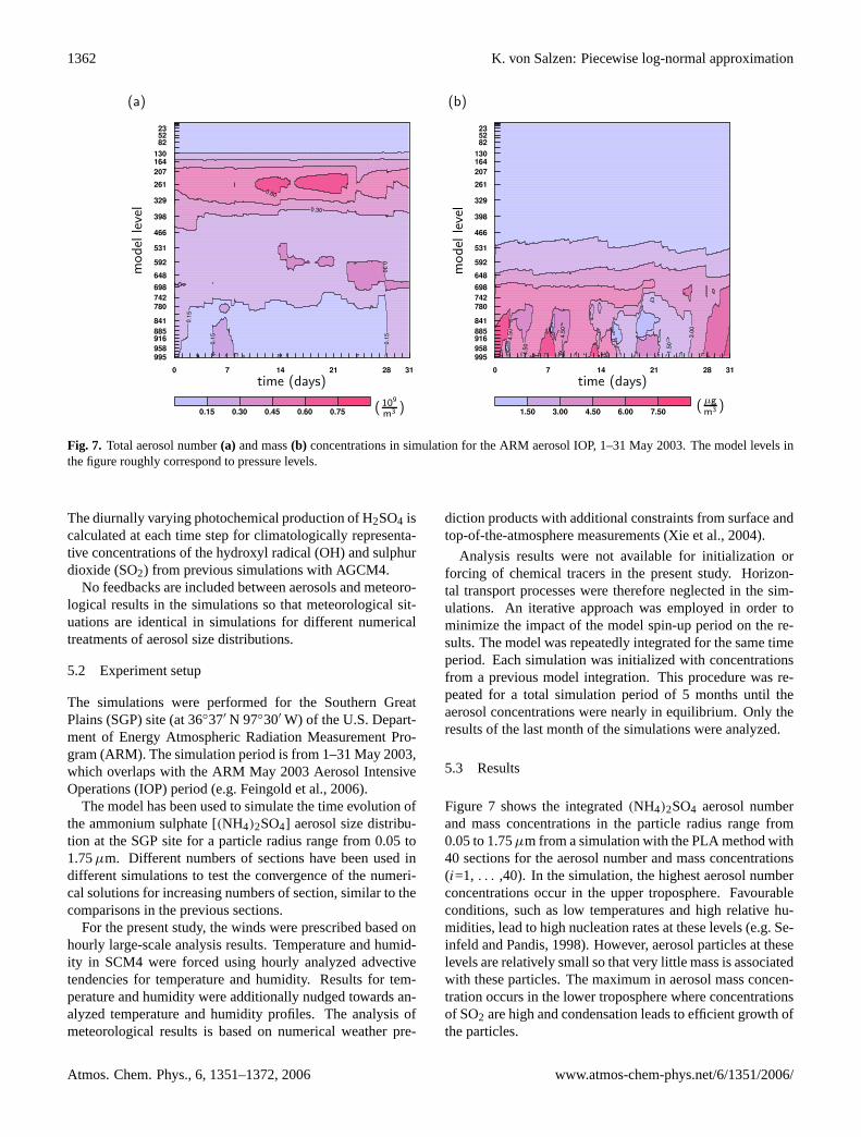
lFig. 7. Total aerosol number (a) and mass (b) concentrations in simulation for the ARM aerosol IOP, May 1-31, 2003. The model levels inthe figure roughly correspond to pressure levels.

to 1.75µm from a simulation with the PLA method with40 sections for the aerosol number and mass concentrations(i=1,. . . ,40). In the simulation, the highest aerosol numberconcentrations occur in the upper troposphere. Favourableconditions, such as low temperatures and high relative hu-midities, lead to high nucleation rates at these levels (e.g. Se-infeld and Pandis, 1998). However, aerosol particles at theselevels are relatively small so that very little mass is associatedwith these particles. The maximum in aerosol mass concen-tration occurs in the lower troposphere where concentrationsof SO2 are high and condensation leads to efficient growthof the particles.

The simulated concentrations are quite variable in time.Most of the variability in the concentrations arises from in-termittent wet deposition events. Simulated wet depositionrates are particularly high during the time period May 14 -24 (Fig. 8). A large fraction of the precipitation results fromdeep convection in the simulation.

Variations in the magnitudes of the sources and sinks ofaerosols are also connected to variations in the sizes of theaerosol particles (Fig. 9 a). A single size mode is simulatedfor the aerosol mass, corresponding to the particle accumu-lation mode in the atmosphere. The deposition of aerosolsdoes not directly lead to any noticeable changes in particlesize. However, the model typically predicts increases in par-ticle size during the time periods following large wet depo-sition events. This is presumably partly caused by a reducedtotal aerosol surface area. Consequently, the condensationof H2SO4 onto the aerosol particles that have not been re-moved by wet deposition is more efficient compared to thetime period before the event. Additionally, the reduction intotal surface area leads to increased nucleation rates duringthe time period following large wet deposition events [see

Eq. (A3)] which eventually leads to the re-establishment ofan accumulation mode that more or less resembles the modethat existed prior the wet deposition event.

There is also some evidence for increased production ofsmall particles after wet deposition events from the resultsfor the aerosol number size distribution in Fig. 10 a. An ad-ditional mode occurs between aboutDp = 0.1 and 0.2µm inthe simulations during these time periods.

As already mentioned, the primary purpose of the simu-lations is to test the performance of the PLA method and tocompare results from this method with results from the mod-ified TFL and SMB approaches. Results in Figs. 9 and 10serve as an illustration of the approach in this study.

The most accurate simulations of the aerosol processeswere obtained from control simulations with a total of 80aerosol tracers for the PLA (e.g. Fig. 9 a), the modified TFL(e.g. Fig. 9 c), and SMB (e.g. Fig. 9 e) methods, correspond-ing to 40 sections for the PLA and modified TFL methodsand 80 sections for the SMB approach. Results of the con-trol simulations agree very well with each other in terms ofconcentrations and sizes of the particles and their timing.

However, results of the comparison in Sections 3 and 4indicate that the accuracy of the SMB approach is systemat-ically lower than the accuracy of the PLA method, even atthese relatively large number of sections (e.g. Fig. 4). Thisexplains why results using the SMB approach are character-ized by slightly weaker maxima of the aerosol mass size dis-tribution compared to the results of the PLA and modifiedTFL methods. Also note that, in contrast to the other results,results for the aerosol number size distribution for the SMBapproach in Fig. 10 e are diagnostic results (as previouslydescribed).

Results displayed in Figs. 9 and 10, a, c, and e give evi-

Fig. 7. Total aerosol number(a) and mass(b) concentrations in simulation for the ARM aerosol IOP, 1–31 May 2003. The model levels inthe figure roughly correspond to pressure levels.

The diurnally varying photochemical production of H2SO4 iscalculated at each time step for climatologically representa-tive concentrations of the hydroxyl radical (OH) and sulphurdioxide (SO2) from previous simulations with AGCM4.

No feedbacks are included between aerosols and meteoro-logical results in the simulations so that meteorological sit-uations are identical in simulations for different numericaltreatments of aerosol size distributions.

5.2 Experiment setup

The simulations were performed for the Southern GreatPlains (SGP) site (at 36◦37′ N 97◦30′ W) of the U.S. Depart-ment of Energy Atmospheric Radiation Measurement Pro-gram (ARM). The simulation period is from 1–31 May 2003,which overlaps with the ARM May 2003 Aerosol IntensiveOperations (IOP) period (e.g.Feingold et al., 2006).

The model has been used to simulate the time evolution ofthe ammonium sulphate [(NH4)2SO4] aerosol size distribu-tion at the SGP site for a particle radius range from 0.05 to1.75µm. Different numbers of sections have been used indifferent simulations to test the convergence of the numeri-cal solutions for increasing numbers of section, similar to thecomparisons in the previous sections.

For the present study, the winds were prescribed based onhourly large-scale analysis results. Temperature and humid-ity in SCM4 were forced using hourly analyzed advectivetendencies for temperature and humidity. Results for tem-perature and humidity were additionally nudged towards an-alyzed temperature and humidity profiles. The analysis ofmeteorological results is based on numerical weather pre-

diction products with additional constraints from surface andtop-of-the-atmosphere measurements (Xie et al., 2004).

Analysis results were not available for initialization orforcing of chemical tracers in the present study. Horizon-tal transport processes were therefore neglected in the sim-ulations. An iterative approach was employed in order tominimize the impact of the model spin-up period on the re-sults. The model was repeatedly integrated for the same timeperiod. Each simulation was initialized with concentrationsfrom a previous model integration. This procedure was re-peated for a total simulation period of 5 months until theaerosol concentrations were nearly in equilibrium. Only theresults of the last month of the simulations were analyzed.

5.3 Results

Figure 7 shows the integrated(NH4)2SO4 aerosol numberand mass concentrations in the particle radius range from0.05 to 1.75µm from a simulation with the PLA method with40 sections for the aerosol number and mass concentrations(i=1, . . . ,40). In the simulation, the highest aerosol numberconcentrations occur in the upper troposphere. Favourableconditions, such as low temperatures and high relative hu-midities, lead to high nucleation rates at these levels (e.g.Se-infeld and Pandis, 1998). However, aerosol particles at theselevels are relatively small so that very little mass is associatedwith these particles. The maximum in aerosol mass concen-tration occurs in the lower troposphere where concentrationsof SO2 are high and condensation leads to efficient growth ofthe particles.


K. von Salzen: Piecewise log-normal approximation 1363K. von Salzen: Piecewise log-normal approximation 13

(a)

num

ber

sourc

eflux

(10

9

m2h)

time (days)

(b)

time (days)

mas

sso

urc

eflux

(µg

m2h)

Fig. 8. Sources and sinks of column-integrated aerosol number (a) and mass (b) concentrations during the simulation. Sources are nucleation(pink lines), condensation (red line). Sinks are wet deposition (blue lines) and gravitational settling (green lines).

dence that the solutions from the different methods have con-verged to very nearly the same solution. It therefore appearsto be appropriate to select results from one of the differentmethods at a large number of sections and to use these re-sults as a reference in comparisons with simulations at lownumber of sections. This allows quantitative comparisonsof the performance of each method for different number ofsections, similar to the comparisons to an exact solution inSections 3 and 4. However, in contrast to previous sections,this approach circumvents the use of an exact solution as areference. In the following, results from the simulation withthe PLA method in Figs. 9 and 10 a are used as a reference.

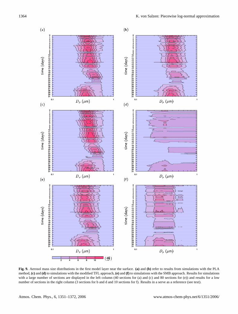
The accuracy of the PLA method depends only weakly onthe number of sections in the simulation. Results for 3 sec-tions (i.e. 6 tracers) with the PLA method are still quite sim-ilar to the reference (Figs. 9 and 10 b). The main differencesare slightly weaker maxima and broader size spectra.

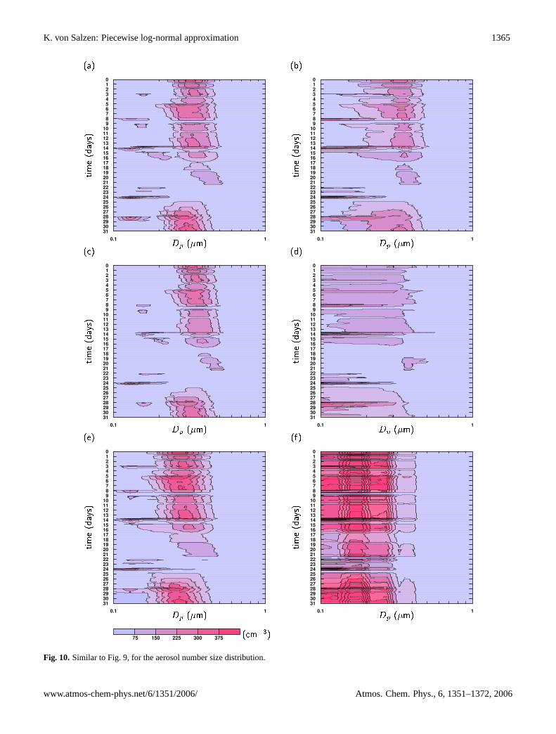
In contrast, there is a marked reduction in the quality ofthe results of the modified TFL and SMB approach for a re-duced number of sections. A simulation with 6 aerosol trac-ers (modified TFL approach) respectively 10 aerosol tracers(SMB approach) produces much broader size distributionsand therefore reveals very little about the temporal evolutionin particle size as apparent in results of the reference experi-ment (Fig. 9 d and f compared to Fig. 9 a). The number sizedistributions are shifted towards much smaller particle sizescompared to the reference simulation. The two distinct par-ticle size modes that are apparent in Fig. 10 a, c, and e nowappear as one single mode.

Artifacts such as those simulated for the SMB approachare typical of the upstream method, which has been usedfor the discretization of the condensation process for thisap-proach (see Appendix A.3). This method is only first-orderaccurate and thus tends to produce strong numerical diffusion(e.g. Bott, 1989). The introduction of the polynomial approx-

imation approach (Section 3) should lead to improvementsregarding the treatment of particle growth. However, as al-ready shown in Section 3, this method would only be usefulfor relatively well resolved size distributions and would notlead to conservation of aerosol number in the simulation.

Results of the SMB approach for 10 sections (Figs. 9 and10 f) have an appreciably lower accuracy than the results ofthe PLA method for 3 sections (Figs. 9 and 10 b). This givesevidence that the application of the SMB method in inter-active simulations of aerosol dynamical processes leads tolarger errors compared to what might be expect from theresults in Section 3. Comparisons in that section showedthat PLA and SMB methods performed about equally wellat these numbers of sections.

In analogy to the discussion in Sections 3 and 4, Fig. 11shows rms differences for simulations with the PLA, modi-fied TFL, and SMB methods for different simulations withdifferent number of sections (i.e. 1, 3, 10, 40, and 80 sec-tions). Similar to Figs. 9 and 10, the accuracy of the resultsgenerally increases with increasing number of sections forall methods. However, the increase is less monotonic than inFig. 4 because of a lower number of cases and the fact thatsection-integrated number and mass concentrations are notprescribed for the current results.

The PLA method produces a systematically higher accu-racy than the SMB method. The same is true in comparisonto the modified TFL approach, except for results for 10 sec-tions, which give similar rms differences.

The difference in accuracy between the double-momentmethods (i.e. PLA and modified TFL) and the SMB methodis more apparent for the aerosol number concentration than itis for the aerosol mass concentration owing to the fact that theaerosol number concentration is a purely diagnostic quantityin the context of the SMB approach [Eq. (A7)] whereas it is

Fig. 8. Sources and sinks of column-integrated aerosol number(a) and mass(b) concentrations during the simulation. Sources are nucleation(pink lines), condensation (red line). Sinks are wet deposition (blue lines) and gravitational settling (green lines).

The simulated concentrations are quite variable in time.Most of the variability in the concentrations arises from in-termittent wet deposition events. Simulated wet depositionrates are particularly high during the time period 14–24 May(Fig. 8). A large fraction of the precipitation results fromdeep convection in the simulation.

Variations in the magnitudes of the sources and sinks ofaerosols are also connected to variations in the sizes of theaerosol particles (Fig.9a). A single size mode is simulatedfor the aerosol mass, corresponding to the particle accumu-lation mode in the atmosphere. The deposition of aerosolsdoes not directly lead to any noticeable changes in particlesize. However, the model typically predicts increases in par-ticle size during the time periods following large wet depo-sition events. This is presumably partly caused by a reducedtotal aerosol surface area. Consequently, the condensationof H2SO4 onto the aerosol particles that have not been re-moved by wet deposition is more efficient compared to thetime period before the event. Additionally, the reduction intotal surface area leads to increased nucleation rates duringthe time period following large wet deposition events (seeEq.A3) which eventually leads to the re-establishment of anaccumulation mode that more or less resembles the mode thatexisted prior the wet deposition event.

There is also some evidence for increased production ofsmall particles after wet deposition events from the resultsfor the aerosol number size distribution in Fig.10a. An addi-tional mode occurs between aboutDp=0.1 and 0.2µm in thesimulations during these time periods.

As already mentioned, the primary purpose of the simu-lations is to test the performance of the PLA method and to

compare results from this method with results from the mod-ified TFL and SMB approaches. Results in Figs.9 and10serve as an illustration of the approach in this study.

The most accurate simulations of the aerosol processeswere obtained from control simulations with a total of 80aerosol tracers for the PLA (e.g. Fig.9a), the modified TFL(e.g. Fig.9c), and SMB (e.g. Fig.9e) methods, correspond-ing to 40 sections for the PLA and modified TFL methodsand 80 sections for the SMB approach. Results of the con-trol simulations agree very well with each other in terms ofconcentrations and sizes of the particles and their timing.

However, results of the comparison in Sects.3 and4 indi-cate that the accuracy of the SMB approach is systematicallylower than the accuracy of the PLA method, even at these rel-atively large number of sections (e.g. Fig.4). This explainswhy results using the SMB approach are characterized byslightly weaker maxima of the aerosol mass size distributioncompared to the results of the PLA and modified TFL meth-ods. Also note that, in contrast to the other results, results forthe aerosol number size distribution for the SMB approach inFig. 10e are diagnostic results (as previously described).

Results displayed in Figs.9 and10a, c, and e give evidencethat the solutions from the different methods have convergedto very nearly the same solution. It therefore appears to beappropriate to select results from one of the different meth-ods at a large number of sections and to use these results as areference in comparisons with simulations at low number ofsections. This allows quantitative comparisons of the perfor-mance of each method for different number of sections, sim-ilar to the comparisons to an exact solution in Sects.3 and4. However, in contrast to previous sections, this approach


1364 K. von Salzen: Piecewise log-normal approximation14 K. von Salzen: Piecewise log-normal approximation(a)

Dp (�m)time(days)

(b)

Dp (�m)time(days)

( )

Dp (�m)time(days)

(d)

Dp (�m)time(days)

(e)

Dp (�m)time(days)

(f)

Dp (�m)time(days)

(�gm3 )Fig. 9. Aerosol mass size distributions in the first model layer nearthe surface. a and b refer to results from simulations with the PLAmethod, c and d to simulations with the modified TFL approach,e and f to simulations with the SMB approach. Results for simulations witha large number of sections are displayed in the left column (40 sections for a and c and 80 sections for e) and results for a low number ofsections in the right column (3 sections for b and d and 10 sections for f). Results in a serve as a reference (see text).

Fig. 9. Aerosol mass size distributions in the first model layer near the surface.(a) and(b) refer to results from simulations with the PLAmethod,(c) and(d) to simulations with the modified TFL approach,(e)and(f) to simulations with the SMB approach. Results for simulationswith a large number of sections are displayed in the left column (40 sections for (a) and (c) and 80 sections for (e)) and results for a lownumber of sections in the right column (3 sections for b and d and 10 sections for f). Results in a serve as a reference (see text).


K. von Salzen: Piecewise log-normal approximation 1365K. von Salzen: Piecewise log-normal approximation 15(a)

Dp (�m)time(days)

(b)

Dp (�m)time(days)

( )

Dp (�m)time(days)

(d)

Dp (�m)time(days)

(e)

Dp (�m)time(days)

(f)

Dp (�m)time(days)

( m�3)Fig. 10. Similar to Fig. 9, for the aerosol number size distribution.Fig. 10. Similar to Fig.9, for the aerosol number size distribution.



circumvents the use of an exact solution as a reference. In thefollowing, results from the simulation with the PLA methodin Figs.9a and10a are used as a reference.

The accuracy of the PLA method depends only weakly onthe number of sections in the simulation. Results for 3 sec-tions (i.e. 6 tracers) with the PLA method are still quite simi-lar to the reference (Figs.9b and10b). The main differencesare slightly weaker maxima and broader size spectra.

In contrast, there is a marked reduction in the quality ofthe results of the modified TFL and SMB approach for a re-duced number of sections. A simulation with 6 aerosol trac-ers (modified TFL approach) respectively 10 aerosol tracers(SMB approach) produces much broader size distributionsand therefore reveals very little about the temporal evolutionin particle size as apparent in results of the reference experi-ment (Figs.9d and f compared to Fig.9a). The number sizedistributions are shifted towards much smaller particle sizescompared to the reference simulation. The two distinct par-ticle size modes that are apparent in Figs.10a, c, and e nowappear as one single mode.

Artifacts such as those simulated for the SMB approachare typical of the upstream method, which has been usedfor the discretization of the condensation process for this ap-proach (see Appendix A3). This method is only first-orderaccurate and thus tends to produce strong numerical diffu-sion (e.g.Bott, 1989). The introduction of the polynomialapproximation approach (Sect.3) should lead to improve-ments regarding the treatment of particle growth. However,as already shown in Sect.3, this method would only be use-ful for relatively well resolved size distributions and wouldnot lead to conservation of aerosol number in the simulation.

Results of the SMB approach for 10 sections (Figs.9f and10f) have an appreciably lower accuracy than the results ofthe PLA method for 3 sections (Figs.9b and10b). This givesevidence that the application of the SMB method in inter-active simulations of aerosol dynamical processes leads tolarger errors compared to what might be expect from the re-sults in Sect.3. Comparisons in that section showed that PLAand SMB methods performed about equally well at thesenumbers of sections.

In analogy to the discussion in Sects.3 and 4, Fig. 11shows rms differences for simulations with the PLA, mod-ified TFL, and SMB methods for different simulations withdifferent number of sections (i.e. 1, 3, 10, 40, and 80 sec-tions). Similar to Figs.9 and10, the accuracy of the resultsgenerally increases with increasing number of sections forall methods. However, the increase is less monotonic than inFig. 4 because of a lower number of cases and the fact thatsection-integrated number and mass concentrations are notprescribed for the current results.

The PLA method produces a systematically higher accu-racy than the SMB method. The same is true in comparisonto the modified TFL approach, except for results for 10 sec-tions, which give similar rms differences.

The difference in accuracy between the double-momentmethods (i.e. PLA and modified TFL) and the SMB methodis more apparent for the aerosol number concentration than itis for the aerosol mass concentration owing to the fact that theaerosol number concentration is a purely diagnostic quantityin the context of the SMB approach (Eq.A7) whereas it ispredicted in the simulations with the double-moment meth-ods.

Similar to the conclusion in Sect.3, the accuracy of theresults with the PLA method is only weakly sensitive to thechoice ofψm,i (Fig. 11).

5.4 Comparison with observations

It is interesting to compare the results of the simulationsin Fig. 9 to observations at the SGP site during the ARMAerosol IOP. An optical particle counter (OPC, Particle Mea-suring Systems Model PCASP-X) provided size distribu-tion data in 31 size classes for particle diameters between0.1 and 10µm (Sheridan et al., 2001). The aerosol samplestream that enters the OPC is heated to a relative humidityof 40% (or less) so that the effect of aerosol water is negli-gible. This allows a direct comparison between the observedand simulated size distributions. For the current study, theobserved aerosol number concentrations in each size classwere converted into an aerosol mass size distribution basedon the assumption of spherical particles with a density of1.769 kg m−3.

Observations are available for limited time periods duringthe IOP. Hourly average results for these time periods areshown in Fig.12. Similar to the simulations (Fig.9), a sin-gle particle mode has been observed in the range from 0.1 to1µm. Also, the maxima in the aerosol size distribution occurat similar particle sizes. However, the observed size distribu-tions are considerably broader and more variable. It is likelythat at least part of the differences are caused by the omis-sion of horizontal transport of aerosols. Other likely causesare the omission of aerosol in-cloud production, coagulation,contributions of non-sulphate aerosols, as well the simplifiedtreatments of wet deposition and photochemical productionof H2SO4 in the simulations. Although the parameterizedphysics is incomplete, the results in Fig.11 give evidencethat the PLA method provides a much more accurate and ef-ficient platform for aerosol modelling than the SMB method.

6 Conclusions

Aerosol physical and chemical processes generally dependon aerosol number, mass, and other moments of the aerosolsize distribution. Currently, various models predict aerosolmass based on numerical approaches that do not guaranteecontinuity of aerosol number or other moments. A vari-ety of multi-moment schemes has also been proposed foruse in atmospheric models. However, there is no apparent


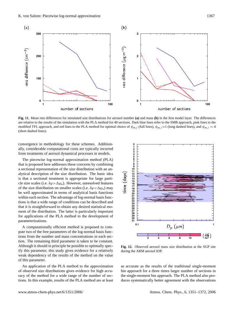
K. von Salzen: Piecewise log-normal approximation 136716 K. von Salzen: Piecewise log-normal approximation(a)

rmsdi�eren e( m�3 )

number of se tions

(b)


Fig. 11. Mean rms differences for simulated size distributions for aerosol number (a) and mass (b) in the first model layer. The differencesare relative to the results of the simulation with the PLA method for 40 sections. Dark blue lines refer to the SMB approach, pink lines tothe modified TFL approach, and red lines to the PLA method for optimal choice ofψm,i (full lines), ψm,i = 1 (long dashed lines), andψm,i = 4 (short dashed lines).

predicted in the simulations with the double-moment meth-ods.

Similar to the conclusion in Section 3, the accuracy of theresults with the PLA method is only weakly sensitive to thechoice ofψm,i (Fig. 11).


It is interesting to compare the results of the simulations in(Fig. 9) to observations at the SGP site during the ARMAerosol IOP. An optical particle counter (OPC, Particle Mea-suring Systems Model PCASP-X) provided size distributiondata in 31 size classes for particle diameters between 0.1and 10µm (Sheridan et al., 2001). The aerosol samplestream that enters the OPC is heated to a relative humidityof 40% (or less) so that the effect of aerosol water is negli-gible. This allows a direct comparison between the observedand simulated size distributions. For the current study, theobserved aerosol number concentrations in each size classwere converted into an aerosol mass size distribution basedon the assumption of spherical particles with a density of1.769kg m−3.

Observations are available for limited time periods duringthe IOP. Hourly average results for these time periods areshown in Fig. 12. Similar to the simulations (Fig. 9), a sin-gle particle mode has been observed in the range from 0.1 to1µm. Also, the maxima in the aerosol size distribution occurat similar particle sizes. However, the observed size distribu-tions are considerably broader and more variable. It is likelythat at least part of the differences are caused by the omis-sion of horizontal transport of aerosols. Other likely causesare the omission of aerosol in-cloud production, coagulation,

Dp (�m) (�gm3 )time(days)

Fig. 12. Observed aerosol mass size distribution at the SGP siteduring the ARM aerosol IOP.

contributions of non-sulphate aerosols, as well the simplifiedtreatments of wet deposition and photochemical productionof H2SO4 in the simulations. Although the parameterizedphysics is incomplete, the results in Fig. 11 give evidencethat the PLA method provides a much more accurate and ef-ficient platform for aerosol modelling than the SMB method.

Fig. 11. Mean rms differences for simulated size distributions for aerosol number(a) and mass(b) in the first model layer. The differencesare relative to the results of the simulation with the PLA method for 40 sections. Dark blue lines refer to the SMB approach, pink lines to themodified TFL approach, and red lines to the PLA method for optimal choice ofψm,i (full lines),ψm,i=1 (long dashed lines), andψm,i = 4(short dashed lines).

convergence in methodology for these schemes. Addition-ally, considerable computational costs are typically incurredfrom treatments of aerosol dynamical processes in models.

The piecewise log-normal approximation method (PLA)that is proposed here addresses these concerns by combininga sectional representation of the size distribution with an an-alytical description of the size distribution. The basic ideais that a sectional treatment is appropriate for large parti-cle size scales (i.e.δϕ>1ϕ?). However, unresolved featuresof the size distribution on smaller scales (i.e.δϕ<1ϕ?) maybe well approximated in terms of analytical basis functionswithin each section. The advantage of log-normal basis func-tions is that a wide range of conditions can be described andthat it is straightforward to obtain any desired statistical mo-ment of the distribution. The latter is particularly importantfor applications of the PLA method to the development ofparameterizations.

A computationally efficient method is proposed to com-pute two of the free parameters of the log-normal basis func-tions from the number and mass concentrations in each sec-tion. The remaining third parameter is taken to be constant.Although it should in principle be possible to optimally spec-ify this parameter, this study gives evidence for a relativelyweak dependency of the results of the method on the valueof this parameter.

An application of the PLA method to the approximationof observed size distributions gives evidence for high accu-racy of the method for a wide range of the number of sec-tions. In this example, results of the PLA method are at least

16 K. von Salzen: Piecewise log-normal approximation(a)rmsdi�eren e( m�3 )

number of se tions

(b)


Fig. 11. Mean rms differences for simulated size distributions for aerosol number (a) and mass (b) in the first model layer. The differencesare relative to the results of the simulation with the PLA method for 40 sections. Dark blue lines refer to the SMB approach, pink lines tothe modified TFL approach, and red lines to the PLA method for optimal choice ofψm,i (full lines), ψm,i = 1 (long dashed lines), andψm,i = 4 (short dashed lines).

predicted in the simulations with the double-moment meth-ods.

Similar to the conclusion in Section 3, the accuracy of theresults with the PLA method is only weakly sensitive to thechoice ofψm,i (Fig. 11).


It is interesting to compare the results of the simulations in(Fig. 9) to observations at the SGP site during the ARMAerosol IOP. An optical particle counter (OPC, Particle Mea-suring Systems Model PCASP-X) provided size distributiondata in 31 size classes for particle diameters between 0.1and 10µm (Sheridan et al., 2001). The aerosol samplestream that enters the OPC is heated to a relative humidityof 40% (or less) so that the effect of aerosol water is negli-gible. This allows a direct comparison between the observedand simulated size distributions. For the current study, theobserved aerosol number concentrations in each size classwere converted into an aerosol mass size distribution basedon the assumption of spherical particles with a density of1.769kg m−3.

Observations are available for limited time periods duringthe IOP. Hourly average results for these time periods areshown in Fig. 12. Similar to the simulations (Fig. 9), a sin-gle particle mode has been observed in the range from 0.1 to1µm. Also, the maxima in the aerosol size distribution occurat similar particle sizes. However, the observed size distribu-tions are considerably broader and more variable. It is likelythat at least part of the differences are caused by the omis-sion of horizontal transport of aerosols. Other likely causesare the omission of aerosol in-cloud production, coagulation,

Dp (�m) ( �gm3 )time(days)


contributions of non-sulphate aerosols, as well the simplifiedtreatments of wet deposition and photochemical productionof H2SO4 in the simulations. Although the parameterizedphysics is incomplete, the results in Fig. 11 give evidencethat the PLA method provides a much more accurate and ef-ficient platform for aerosol modelling than the SMB method.


as accurate as the results of the traditional single-momentbin approach for a three times larger number of sections inthe single-moment bin approach. The PLA method also pro-duces systematically better agreement with the observations



than double-moment bin schemes based on the work byTziv-ion et al.(1987) or approximations in terms of polynomials.

The superior performance of the PLA method comparedto the single- and double-moment bin methods is even moreapparent from applications of the methods to prognostic sim-ulations with a single column model. The processes includedin these simulations are vertical transport, nucleation, con-densation, gravitational settling, and wet deposition for am-monium sulphate aerosol.

Although the PLA method performs very well in applica-tions to observed size distributions, the condensation equa-tion, and single column model simulations in this study, itclearly is not possible to prove the efficiency of the methodbased on these tests alone. It will be necessary to study theperformance of the method in additional applications to ac-tivation and chemical modifications in clouds, coagulation,etc. for more general conclusions. These tests will be donein the future. Despite the limited number of applications ofthe PLA method in the current study, the results appear tobe useful tests of the method owing to the importance of thestudied processes in the atmosphere and the difficulties toefficiently model these processes based on commonly con-sidered single- and double-moment methods.

Results from additional tests of the method and imple-mentations in the CCCma Atmospheric General CirculationModel will be reported in subsequent publications.

Appendix A

Parameterization of nucleation and condensation

The growth of aerosol particles due to condensation of sul-phuric acid (H2SO4) and ammonia (NH3) can be expressedusing Fick’s law (e.g.Seinfeld and Pandis, 1998). NH3 istypically highly abundant in the troposphere (e.g.Dentenerand Crutzen, 1994). Hence, it can be safely assumed thatcondensation of NH3 leads to nearly immediate and completereaction of H2SO4 to (NH4)2SO4 in the particles. Further-more, the concentration of H2SO4 is approximately nil at thesurface of the particles. This appears to be a good approx-imation owing to the very low volatility of H2SO4. Underthese assumptions, the time evolution of the particle radiusRpd for dry (i.e. solid) aerosol can be expressed by

dRpd

dt=cgC

Rpd, (A1)

with the concentrationC of H2SO4 (in kg m−3) and

cg =

(M(NH4)2SO4

MH2SO4

)DF Ae1ϕw

ρpd.

M(NH4)2SO4 andMH2SO4 refer to the molecular weights of(NH4)2SO4 and H2SO4 (in kg mol−1). ρpd denotes the den-sity of the dry aerosol (in kg m−3). D represents the diffusiv-ity of H2SO4 in air (in m2 s−1). F andA are dimensionless

and size-dependent factors which account for non-continuumeffects and imperfect surface accommodation (von Salzenet al., 2000). Note that unity is used for the mass accom-modation coefficient inA in this study. This value appears tobe in qualitatively good agreement with results of recent the-oretical and laboratory studies (Kulmala and Wagner, 2001).Finally, 1ϕw refers to the difference between wet and dryparticle size owing to the aerosol water content, i.e.

1ϕw = ln

(Rpw

Rpd

), (A2)

for dry and wet particle radii,Rpd andRpw. In this study,1ϕw has been determined from thermodynamic equilibriumfor mean concentrations in each section (Gong et al., 2003).

The time evolution of the H2SO4 concentration due to gas-phase production, nucleation, and condensation can be de-scribed by:

dC

dt= P − kCs

−4π C D∑i

∫ ϕi+1/2

ϕi−1/2

F ARpw n (ϕ) dϕ . (A3)

In Eq. (A3), P represents the production of H2SO4 from oxi-dation of sulphur dioxide by the hydroxyl radical (Stockwelland Calvert, 1983). The following term represents the lossesfrom binary homogeneous nucleation for H2SO4 and watervapour, with temperature and humidity dependent parame-tersk ands (e.g.von Salzen et al., 2000).

The last term in Eq. (A3) represents the condensation ofH2SO4. It follows from Eq. (A1) from integration over thesize distribution.Rpw is calculated from1ϕw and the dryparticle sizeRpd=R0 exp(ϕ) (Eq.A2). Note that the numbersize distribution in the integral in Eq. (A3) is a function ofthe dry particle size with constant section boundariesϕi±1/2.This approach is sometimes used in aerosol models to in-crease the numerical accuracy of simulations with varyingaerosol water contents. With this approach, the concentra-tions of the total aerosol (including water) can be easily di-agnosed based on the results for the size distribution for dryparticles and Eq. (A2).

Sensitivity tests give evidence for rapid adjustment ofC

toward equilibrium for a wide range of atmospheric condi-tions that exist in large-scale atmospheric models. On theother hand, changes ofP , k, s, D, F , A, 1ϕw, andn(ϕ)are typically much smaller compared to changes inC over amodel time step (1t≈30 min). Hence, Eq. (A3) is integratedunder the assumption of a constant aerosol size distributionduring the time step.

A1 Application of PLA method

In order to simplify the numerical approach for the PLAmethod, the size-dependence of the termFA in Eqs. (A3)



and (A1) is approximated by

F A ≈ (F A)i−1/2

+(F A)i+1/2 − (F A)i−1/2

eϕi+1/2 − eϕi−1/2

(eϕ − eϕi−1/2

)(A4)

for ϕi−1/2≤ϕ≤ϕi+1/2.Equation (A1) is used to obtain a linearized expression for

the change in dry particle radius during a single model timestep, i.e.

Rpd(t0 +1t) = Rpd(t0)+cg(t0)

Rpd(t0)

∫ t0+1t

t0

C dt , (A5)

where the integral results from integration of Eq. (A3) asdescribed in the previous section. This procedure ensuresthat the change in particle mass from condensation of H2SO4matches the change in H2SO4 concentration from integrationof Eq. (A3).

Calculations for each section according to Eq. (A5) are fol-lowed by a remapping procedure so that the section bound-aries for dry particles remain unchanged at each time step inthe model. The remapping procedure is a straightforward in-tegration over the size distribution for the particle radii aftercondensation (Eq.A5), based on Eqs. (4) and (5).

For the treatment of nucleation it is assumed that thesize distribution of the freshly produced particles is a delta-function for a particle size corresponding to the size of thesmallest particles in the first sectioni=1. The amount ofthose particles is determined from integration of the nucle-ation term in Eq. (A3) over1t .

A2 Application of modified TFL approach

In analogy to Eq. (14), size distributions can be defined forany required moment of the distribution, i.e.(

dµkdϕ

)mTFL,i

= Rkp,i−1/2 am,i

(ϕi+1/2 − ϕ

1ϕ?

)+ Rkp,i+1/2 bm,i

(ϕ − ϕi−1/2

1ϕ?

), (A6)

for the same coefficientsam,i andbm,i as in Eq. (14).Equation (A6) is used to solve Eq. (A3). Similar to

the PLA method, Eq. (A4) is used to account for the size-dependence of the termFA in Eq. (A3).

The approximated number and mass size distributions ac-cording to Eqs. (13) and (14), violate the fundamental rela-tionship

dM

dϕ= mp

dN

dϕ

for ϕi−1/2<ϕ<ϕi+1/2. However, the approximated numberand mass size distributions satisfy this relationship for parti-cle sizesϕ=ϕi−1/2 andϕi+1/2 for each section (although theresults may differ for adjacent sections). It is therefore desir-able to apply Eq. (A5) to particles with sizes corresponding

to the boundaries of the sections. This leads to new num-ber and mass size distributions for these particles after con-densation. By using the simplifying assumption that particlegrowth does not cause the size distributions to become non-linear, these results can then be linearly interpolated to givenew size distributions for all other particles. Similar to theprocedure outlined in Sect. A1, remapping of the size distri-butions onto the original sections and integration yields newaerosol number and mass concentrations for each aerosoltracer.

A3 Application of SMB approach

For the application of the single-moment bin approach, it isassumed that the number size distribution within each sectioncan be approximated by

n (ϕ) ≈Ni

1ϕ?,

for ϕi−1/2≤ϕ≤ϕi+1/2, with

Ni ≈Mi

4π3 ρpd R

30 exp

(3ϕc,i

) , (A7)

and

ϕc,i = ϕi−1/2 +1

21ϕ? . (A8)

It is further assumed that

F ARpw ≈(F ARpw

)i−1/2

+

(F ARpw

)i+1/2 −

(F ARpw

)i−1/2

eϕi+1/2 − eϕi−1/2

(eϕ − eϕi−1/2

)for ϕi−1/2≤ϕ≤ϕi+1/2.

Similar to the application of the PLA method, Eq. (A3)is integrated to obtain the change1C in H2SO4 concentra-tion over1t . Let1Ccnd be the contribution of condensation(i.e. from last term in Eq.A3) to1C. Mass continuity thenimplies that the aerosol mass changes according to

1Mi = −

(M(NH4)2SO4

MH2SO4

)1Ccnd .

for particles withϕi−1/2≤ϕ≤ϕi+1/2 at the beginning of thetime step. A change in aerosol mass from condensationis accompanied by a change in particle size1ϕc,i . 1ϕc,ican be obtained from Eq. (A7) under the assumption thatNi=const.:

1ϕc,i =1

3ln

(1 +

1Mi

Mi

).

On the other hand, section boundaries are not allowed tochange between time steps, similar to the application of thePLA method. This requires a redistribution of mass between



different sections. Hence, the mass concentration at timet=t0+1t is calculated from

M (t0 +1t) = T [M (t0)+1M] ,

whereM and1M are vectors with elementsMi , respec-tively 1Mi . T is a matrix with elements

tij = H(1ϕ−

(i−1/2)j

)H(1ϕ+

(i−1/2)j

)1ϕ+

(i−1/2)j1ϕ?

+ H(1ϕ−

(i+1/2)j

)H(1ϕ+

(i+1/2)j

)1ϕ−

(i+1/2)j1ϕ?

,

with

1ϕ−

(i±1/2)j = ϕt,(i±1/2)j − ϕj−1/2 ,

1ϕ+

(i±1/2)j = ϕj+1/2 − ϕt,(i±1/2)j ,

and

ϕt,(i±1/2)j = ϕi±1/2 −1ϕc,j .

Aerosol mass resulting from nucleation is inserted into thefirst section according the change in H2SO4 concentrationfrom nucleation over1t (Eq.A3).

Appendix B

Parameterization of gravitational settling

The terminal settling velocity of a spherical aerosol particleis

vt =2

9

R2pw ρpw g Cc

µ, (B1)

with the gravitational accelerationg, density of the wetaerosolρpw, and slip correction factor

Cc = 1 +λ

Rpw

[1.257+ 0.4 exp

(−

1.1Rpwλ

)], (B2)

and mean free path of airλ (Seinfeld and Pandis, 1998).In order to simplify the discretization and increase the ef-

ficiency of the numerical solution, the approximation

exp

(−

1.1Rpwλ

)≈ exp

(−

1.1R0 eϕc,i+1ϕw

λ

)is used forϕi−1/2≤ϕ≤ϕi+1/2 in Eq. (B2), with ϕc,i fromEq. (A8).

B1 Application of PLA method

Equation (B1) is used to calculate effective terminal settlingvelocities for particle number (vtn,i) and mass (vtm,i) in eachsectioni from integration over the section, i.e.

vtn,i =1

Ni

∫ ϕw,i+1/2

ϕw,i−1/2

vt n(ϕ −1ϕw) dϕ , (B3)

vtm,i =1

Mi

4π

3ρp,iR

30

∫ ϕw,i+1/2

ϕw,i−1/2

vt e3ϕn(ϕ −1ϕw)dϕ ,(B4)

with ϕw,i±1/2=ϕi±1/2+1ϕw.

B2 Application of modified TFL approach

Equations (B3) and (B4) are also used for the TFL approachfor linearRkpn(ϕ − 1ϕw) according to Eqs. (13), (14), and(A6).

B3 Application of SMB approach

Effective terminal settling velocities are obtained forMi

from Eq. (B1) for Rpw=R0 exp(ϕc,i+1ϕw

).

Acknowledgements.I would like to thank S. Ghan and two otheranonymous reviewers for their very helpful comments. The authorfurther thanks S. Xie for providing the single column modelforcing data and G. Feingold, N. McFarlane, W. Merryfield, andJ. Scinocca for discussions. This research was partially supportedby the Climate Change Action Fund (CCAF) and EnvironmentCanada.

Edited by: G. Feingold

References

Ackermann, I. J., Hass, H., Memmesheimer, M., Ebel, A.,Binkowski, F. S., and Shankar, U.: Modal aerosol dynamicsmodel for Europe: Development and first applications, Atmos.Environ., 32, 2981–2999, 1998.

Binkowski, F. S. and Shankar, U.: The regional particulate mattermodel 1. Model description and preliminary results, J. Geophys.Res., 100, 21 191–21 209, 1995.

Birmili, W., Wiedensohler, A., Heintzenberg, J., and Lehmann, K.:Atmospheric particle number size distribution in central Europe:Statistical relations to air masses and meteorology, J. Geophys.Res., 106, 32 005–32 018, 2001.

Bott, A.: A positive definite advection scheme obtained by nonlin-ear renormalization of the advective fluxes, Mon. Wea. Rev., 117,1006–1015, 1989.

Bott, A.: A flux method for the numerical solution of the stochasticcollection equation, J. Atmos. Sci., 55, 2284–2293, 1998.

Dentener, F. and Crutzen, P. J.: A 3-dimensional model of the globalammonia cycle, J. Atmos. Chem., 19, 331–369, 1994.

Dhaniyala, S. and Wexler, A. S.: Numerical schemes to model con-densation and evaporation of aerosols, Atmos. Environ., 30, 919–928, 1996.

Feingold, G.: Modeling of the first indirect effect: Analysisof measurement requirements, Geophys. Res. Lett., 30, 1997,doi:10.1029/2003GL017967, 2003.

Feingold, G., Furrer, R., Pilewski, P., Remer, L. A., Min, Q., andJonsson, H.: Aerosol indirect effect studies at Southern GreatPlains during the May 2003 intensive operations period, J. Geo-phys. Res., 111, D05514, doi:10.1029/2004JD005648, 2006.

Feller, W.: An introduction to probability theory and its applica-tions, Whiley, New York, 1971.

Gelbard, F.: Modeling multicomponent aerosol particle growth byvapor condensation, Aerosol Sci. Technol., 12, 399–412, 1990.

Gelbard, F. and Seinfeld, J. H.: Simulation of multicomponentaerosol dynamics, J. Colloid Interface Sci., 78, 485–501, 1980.

Gilliani, N. V., Schwartz, S. E., Leaitch, W. R., Strapp, J. W., andIsaac, G. A.: Field observations in continental stratiform clouds:



Partitioning of cloud particles between droplets and unactivatedinterstitial aerosols, J. Geophys. Res., 100, 18 687–18 706, 1995.

Gong, S. L., Barrie, L. A., Blanchet, J.-P., von Salzen, K., Lohmann,U., Lesins, G., Spacek, L., Zhang, L. M., Girard, E., Lin,H., Leaitch, R., Leighton, H., Chylek, P., and Huang, P.:Canadian Aerosol Module: A size-segregated simulation of at-mospheric aerosol processes for climate and air quality mod-els – 1. Module development, J. Geophys. Res., 108, 4007,doi:10.1029/2001JD002002, 2003.

Harrington, D. Y. and Kreidenweis, S. M.: Simulations of sulfateaerosol dynamics – Part II. Model intercomparison, Atmos. En-viron., 32, 1701–1709, 1998.

Jacobson, M. Z.: Development and application of a new air pollu-tion modeling system – II. Aerosol module structure and design,Atmos. Environ., 31, 131–144, 1997.

Kerminen, V.-M. and Wexler, A. S.: Growth laws for atmosphericaerosol particles: An examination of the bimodality of the accu-mulation mode, Atmos. Environ., 29, 3263–3275, 1995.

Kleinman, L. I., Daum, P. H., Imre, D. G., Lee, J. H., Lee, Y.-N., Nunnermacker, L. J., Springston, S. R., Weinstein-Lloyd, J.,and Newman, L.: Ozone production in the New York city urbanplume, J. Geophys. Res., 105, 14 495–14 511, 2000.

Korhonen, H., Lehtinen, K. E. J., Pirjola, L., Napari, I.,and Vehkamaki, H.: Simulation of atmospheric nucle-ation mode: A comparison of nucleation models and sizedistribution representations, J. Geophys. Res., 108, 4471,doi:10.1029/2002JD003305, 2003.

Kulmala, M. and Wagner, P. E.: Mass accommodation and uptakecoefficients - a quantitative comparison, J. Aerosol Sci., 32, 833–841, 2001.

Laprise, R. and Girard, E.: A spectral general circulation modelusing a piecewise-constant finite element representation on a hy-brid vertical coordinate system, J. Climate, 3, 32–52, 1990.

Lohmann, U., von Salzen, N., McFarlane, K., Leighton, H. G., andFeichter, J.: Tropospheric sulphur cycle in the Canadian generalcirculation model, J. Geophys. Res., 104, 26 833–26 858, 1999.

Lurmann, F. W., Wexler, A. S., Pandis, S. N., Musarra, S., Kumar,N., and Seinfeld, J. H.: Modelling urban and regional aerosols– II. Application to California’s south coast air basin, Atmos.Environ., 31, 2695–2715, 1997.

McFarlane, N. A., Scinocca, J. F., Lazare, M., Harvey, R., Verseghy,D., and Li, J.: The CCCma third generation atmospheric generalcirculation model (AGCM3), Internal report, Canadian Centrefor Climate Modelling and Analysis, pp. 23, 2006.

McGraw, R.: Description of aerosol dynamics by the quadraturemethod of moments, Aerosol Sci. Technol., 27, 255–265, 1997.

Meng, Z. Y., Dabdub, D., and Seinfeld, J. H.: Size-resolved andchemically resolved model of atmospheric aerosol dynamics, J.Geophys. Res., 103, 3419–3435, 1998.

Pilinis, C., Capaldo, K. P., Nenes, A., and Pandis, S. N.: MADM– A new multicomponent aerosol dynamics model, Aerosol Sci.Technol., 32, 482–502, 2000.

Remer, L. A., Kaufman, Y. J., and Holben, B. N.: Interannual vari-ation of ambient aerosol characteristics on the east coast of theUnited States, J. Geophys. Res., 104, 2223–2231, 1999.

Russell, L. M. and Seinfeld, J. H.: Size- and composition-resolvedexternally mixed aerosol model, Aerosol Sci. Technol., 28, 403–416, 1998.

Seigneur, C.: A model of sulfate aerosol dynamics in atmospheric

plumes, Atmos. Environ., 16, 2207–2228, 1982.Seigneur, C., Hudischewskyi, A. B., Seinfeld, J. H., Whitby, K. T.,

Whitby, E. R., Brock, J. R., and Barnes, H. M.: Simulation ofaerosol dynamics: A comparative review of mathematical mod-els, Aerosol Sci. Technol., 5, 205–222, 1986.

Seinfeld, J. H. and Pandis, S. N.: Atmospheric chemistry andphysics: From air pollution to climate change, Whiley, NewYork, 1998.

Sheridan, P. J., Delene, D. J., and Ogren, J. A.: Four years of con-tinuous surface aerosol measurements from the Department ofEnergy’s Atmospheric Radiation Measurement Program South-ern Great Plains Cloud and Radiation Testbed site, J. Geophys.Res., 106, 20 735–20 747, 2001.

Stockwell, W. R. and Calvert, J. G.: The mechanism of HO-SO2reaction, Atmos. Environ., 17, 2231–2235, 1983.

Tzivion, S., Feingold, G., and Levin, Z.: An efficient numericalsolution to the stochastic collection equation, J. Atmos. Sci., 44,3139–3149, 1987.

von Salzen, K. and Schlunzen, K. H.: A prognostic physico-chemical model of secondary and marine inorganic multicom-ponent aerosols I. Model description, Atmos. Environ., 33, 767–576, 1999a.

von Salzen, K. and Schlunzen, K. H.: A prognostic physico-chemical model of secondary and marine inorganic multicompo-nent aerosols II. Model tests, Atmos. Environ., 33, 1543–1552,1999b.

von Salzen, K., Leighton, H. G., Ariya, P. A., Barrie, L. A., Gong,S. L., Blanchet, J.-P., Spacek, L., Lohmann, U., and Kleinman,L. I.: Sensitivity of sulphate aerosol size distributions and CCNconcentrations over North America to SOx emissions and H2O2concentrations, J. Geophys. Res., 105, 9741–9765, 2000.

von Salzen, K., McFarlane, N. A., and Lazare, M.: The role ofshallow convection in the water and energy cycles of the atmo-sphere, Climate Dyn., 25, 671–688, doi:10.1007/s00382-005—51-2, 2005.

Warren, D. R. and Seinfeld, J. H.: Simulation of aerosol size distri-bution evolution in systems with simultaneous nucleation, con-densation, and coagulation, Aerosol Sci. Technol., 4, 31–43,1985.

Whitby, E., Stratmann, F., and Wilck, M.: Merging and remappingmodes in modal aerosol dynamics models: A “Dynamic ModeManager”, J. Aerosol Sci., 33, 623–645, 2002.

Whitby, E. R.: Modal aerosol dynamics modeling, Aerosol Sci.Technol., 27, 673–688, 1997.

Whitby, K. T.: The physical characteristics of sulfur aerosols, At-mos. Environ., 12, 135–159, 1978.

Whitby, K. T.: Determination of aerosol growth rates in the atmo-sphere using lumped aerosol dynamics, J. Aerosol Sci., 12, 174–178, 1981.

Wilck, M. and Stratmann, F.: A 2-D multicomponent modal aerosolmodel and its application to laminar flow reactors, J. AerosolSci., 28, 959–972, 1997.

Wilson, J., Cuvelier, C., and Raes, F.: A modeling study of globalmixed aerosol fields, J. Geophys. Res., 106, 34 081–34 108,2001.

Wright, D. L., Kasibhatla, P. S., McGraw, R., and Schwartz, S. E.:Description and evaluation of a six-moment aerosol microphysi-cal module for use in atmospheric chemical transport models, J.Geophys. Res., 106, 20 275–20 291, 2001.



Xie, S., Cederwall, R. T., and Zhang, M.: Developing long-termsingle-column model/cloud system-resolving model forcing datausing numerical weather prediction products constrained by sur-face and top of the atmosphere observations, J. Geophys. Res.,109, D01104, doi:10.1029/2003JD004045, 2004.

Yu, S., Kasibhatla, P. S., Wright, D. L., Schwartz, S. E., and Mc-Graw, R.: Moment-based simulation of microphysical propertiesof sulfate aerosols in the eastern United States: Model descrip-tion, evaluation, and regional analysis, J. Geophys. Res., 108,4353, doi:10.1029/2002JD002890, 2003.

Zender, C. S., Bian, H., and Newman, D.: Mineral dustentrainment and deposition (DEAD) model: Descriptionand 1990s dust climatology, J. Geophys. Res., 108, 4416,doi:10.1029/2002JD002775, 2003.

Zhang, Y., Seigneur, C., Seinfeld, J. H., Jacobson, M. Z., andBinkowski, F. S.: Simulation of aerosol dynamics: A compar-ative review of algorithms used in air quality models, AerosolSci. Technol., 31, 487–514, 1999.

Zhang, Y., Easter, R. C., Ghan, S. J., and Abdul-Razzak,H.: Impact of aerosol size representations on modelingaerosol-cloud interactions, J. Geophys. Res., 107, 4558,doi:10.1029/2001JD001549, 2002.


piecewise log-normal approximation of size distributions

Documents