1

PIER Summer Course on Bayesian Models in Education Research

Review and Overview Howard Seltman July 12+15 2016

I. Some Context and Motivation

a. The Efficacy of the Hedges Correction for Unmodeled Clustering, and Its Generalizations

in Practical Settings by Nathan VanHoudnos, CMU PhD Dissertation, 2014

(http://www.stat.cmu.edu/~nmv/wp-content/uploads/2014/05/vanhoudnos-

dissertation-5-5-2014.pdf).

“The aim of the evidence based education movement is two-fold: (i) to determine the

best practices from scientifically rigorous studies and (ii) to apply those best practices to

educational decision making. To assist the adoption of evidence based practices by US

educators and policy makers, Congress created the What Works Clearinghouse (WWC)

with a mission to evaluate evidence about educational interventions and to disseminate

information about best practices. The WWC synthesizes the results of education

research and publishes these recommendations for use by educators and policy makers.

Throughout its history, however, the evidence based education movement has struggled

with the low quality of education research. For example, a common analytic error made

by education researchers is that an experiment will be designed to randomize entire

schools to treatment and control conditions, but then the experiment will be analyzed

ignoring the grouped nature of the randomization. This error is well known to lead to

invalid conclusions because it overstates the statistical significance of the treatment

effect. The WWC chose to address this common error by attempting to remove the

anti-conservative bias of these misspecified analyses by calculating a correction to the

test statistic.”

b. Revisiting higher education data analysis: A Bayesian perspective by M. Subbiah, M. R.

Srinivasan and S. Shanthi, International Journal of Science and Technology Education

Research, 1(2), 32-38 (2011),

(http://www.academicjournals.org/article/article1379514827_Subbiah%20et%20al.pdf)

Although the English usage is poor, this paper is a nice example of the “Bayesian

Perspective” in practice.

2

II. Review of Principles of Experimental Design

a. IV vs. DV

b. Variable types

c. Causality, confounding, randomization, and internal validity

d. External Validity / Generalizability (not related to sample size!)

e. Construct validity

f. Power and precision (high with high sample size, low variability, and strong treatment

effects)

g. Means models, including interaction

h. Error models to match DV type and correlation pattern

3

III. Background Common to Classical and Bayesian Inference

a. Intuitive definitions of probability

i. Long run frequency

ii. Subjective chance of occurrence

b. Set theory

i. A set is a list of items with no duplicates

ii. If A and B are sets, their union, 𝐴 ∪ 𝐵 is the set of all elements in A, B or both.

It is at least as big as the larger of the two.

iii. If A and B are sets, their intersection, 𝐴 ∩ 𝐵 is the set of all elements in both A

and B. It is no bigger than the smaller of the two.

iv. 𝐴 ⊆ 𝐵 means that A is the same set at B or is only a subset of B.

v. Disjoint sets have no elements in common.

vi. The complement of set A, Ac, is all elements except those in A.

c. Probability axioms and notation

i. Consider a situation with an unknown outcome.

ii. Let the sample space, represent all possible outcomes.

iii. Let represent each specific possible (discrete) elementary outcome.

iv. Let E, an event, represent a specific collection of possible outcomes.

v. Birthday example

vi. 0 ≤ Pr() ≤ 1

vii. Pr()=1

viii. If E1 and E2 are disjoint, then Pr(E1 ᴜ E2) = Pr(E1) + Pr(E2)

4

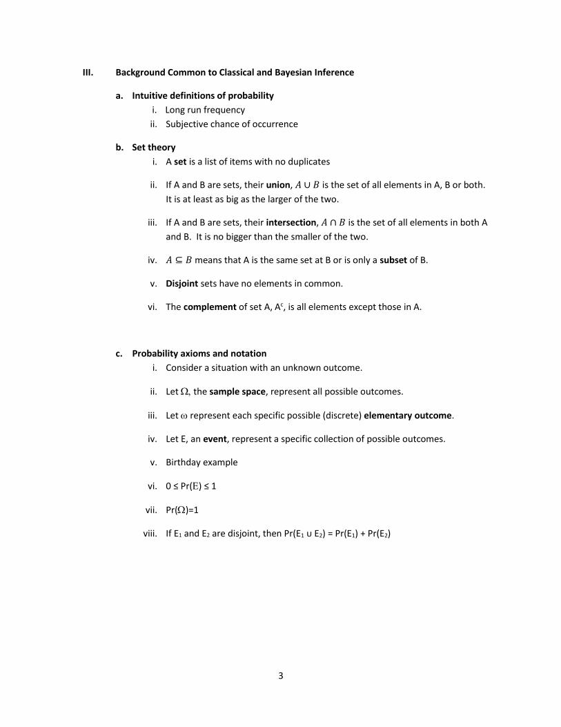
d. Conditional probability

i. The probability that event B will occur given that we know that event A did

occur is called the conditional probability of B given A and is written Pr(B|A).

ii. As a trivial example, if𝐵 ⊆ 𝐴, it is obvious that Pr(A|B)=1.

iii. In general, Pr(𝐵|𝐴) = Pr (𝐴∩𝐵)

Pr (𝐴). This is best thought of as a reduction of the

sample space from to A.

iv. Useful alternative version: Pr(B|A) Pr(A) = Pr(A ∩ B)

v. Partition rule: If sets A1 through Ak partition then

Pr(B) = Pr(B|A1)Pr(A1)+…+Pr(B|Ak) Pr(Ak)

vi. Bayes’ rule (also true and useful for Classical Statistics):

Pr(𝐴|𝐵) = Pr (𝐴 ∩ 𝐵)

Pr (𝐵)=

Pr(𝐵|𝐴) Pr (𝐴)

Pr(𝐵|𝐴) Pr(𝐴) + Pr(𝐵|𝐴𝑐) Pr (𝐴𝑐)

From the above example:

Pr(𝐴|𝐵) = 0.02

0.05=

0.10 ∙0.20

0.10 ∙0.20+ 0.0375 ∙0.80 = 0.40

vii. Statistical models are based on the idea of conditional distributions: we model

the distribution of the DV given each specific combination of IVs.

5

e. A random variable, usually represented by a capital Roman letter such as X or Y, is a

“mapping” from all events to the set of real numbers, ℝ.

i. The population mean or expected value of Y is the weighted average where the

weights are the probabilities of each Y value. This is written E(Y), or often as .

The corresponding quantity in a sample of Y values is the sample mean, �̅�.

ii. The population variance of Y is the weighted average of the squared distances

of the Y values from the population mean. It is a measure of the spread of the Y

values around the mean Y value. It may be written as var(Y) or Y2. The

notation var(Y) can also refer to the sample variance.

iii. Standard deviation is another measure of spread defined as the square root of

the variance of Y. For any distribution no more than 1/k2 of the distribution is

more than k s.d. from E(Y) according to Chebyshev's inequality.

f. Independence: If knowing that event A happened does not change your estimate of the

chance that event B will happen, then A and B are independent (which is very different

from “disjoint”; disjoint events are always dependent).

i. Notation: A B can be read A and B are independent

ii. A B implies Pr(B|A) = Pr(B) and Pr(A|B) = Pr(A)

iii. A B impliesPr(𝐴 ∩ 𝐵) = Pr(𝐴) Pr(𝐵)

iv. Practically, random variables X and Y are independent if knowing one result tells

us nothing about the other: Pr(Y|X=x)=Pr(Y) and Pr(X|Y=y)=Pr(X).

v. The covariance and correlation between two random variables tells how

information about one provides information about the other.

cov(𝑋, 𝑌) = 𝐸[(𝑋 − 𝐸(𝑋))(𝑌 − 𝐸(𝑌)]

cor(𝑋, 𝑌) =cov(𝑋, 𝑌)

sd(𝑋) sd(𝑌)

vi. Correlation is between -1 and 1. Independent variables always have zero

correlation. Correlations of 1 or -1 mean Y can be perfectly predicted from X.

vii. Technical note: The only general case where uncorrelated implies independent

is when X and Y are bivariate Gaussian.

6

g. Properties of combinations of random variables

i. Let X and Y be random variables, and a, b, and c be constants

ii. E(aX + bY + c) = aE(X) + bE(Y) + c

iii. var(aX + bY +c) = a2 var(X) + b2 var(Y) + 2ab cov(X, Y)

iv. E.g., Xi=weight of apple i, Yi = weight of cereal box j. Assume all Xis and Yis are

independent, E(Xi)=100 g, E(Yi)=300 g, var(Xi)=10 g2, var(Yi)=5 g2.

Boxes are packed with a=4 apples and b=2 oranges and each box weighs c=100

g. The mean weight of a box is 4(100) + 2(300) + 100 = 1100 g. The variance of

the weights is 16*10 + 4*5 + 0 = 180 g2, and the s.d. is √180 = 13.4 g. If the

distributions are Gaussian, then 95% of the boxes weigh in the range 1100 +/-

(1.96)13.4 = [1073.7, 1126.3] g.

v. E.g., Xi is the number of opera tickets student i buys, and Yi is the number of

Pirates tickets. Assume E(Xi)=0.5, var(Xi)=0.6, E(Yi) =1.5, var(Yi)=0.8, and

cov(Xi,Yi)=-0.45.

s.d.(Xi) = √0.6 = 0.77, s.d.(Yi) = √0.8 = 0.89, cor(Xi,Yi) = -0.45 / (0.77 * 0.89)

= -0.66. Let Zi = the total number of opera +Pirates tickets as student buys. E(Zi)

= 0.5 + 1.5 = 2, var(Zi) = 0.6 + 0.8 + 2*(-0.45) = 0.5. s.d.(Zi)=0.71.

ii. Specifying probability distributions

i. For discrete outcomes

a. Distribution is defined with a probability mass function (pmf)

b. All possible values are listed, a probability is given for each value, and

these probabilities add to 1.

c. Bernoulli “coin flipping” distribution: Yϵ {0,1}, Pr(Y=1)=,

Pr(Y=0)=1-, ϵ[0,1]

d. The Bernoulli distribution, like most, is actually a family of

distributions, one for each parameter value, .

e. For Bernoulli() we can compute E(Y)= and var(Y)=(1-).

f. The binomial distribution (independent flips of a given coin): The

outcome, Y, is the number of “heads” for n independent flips of a coin

with chance of heads for each flip. E(X)=n, Var(Y)= n The

pmf is Pr(Y = y) = n!

y! (n−y)! 𝜋𝑦 (1 − 𝜋)𝑛−𝑦, where “!” mean

factorial.

7

g. The Poisson distribution: The outcome Y can be thought of as the

count of independent events in a fixed time period. Y can be 0, 1, 2,

…. The family is indexed by the parameter . E(Y)=, var(Y)=. The

pmf is Pr(Y = Y) = λ𝑦𝑒−𝜆

y! where e is Euler’s constant, 2.71828….

h. Other discrete distributions include discrete uniform, negative

binomial, hypergeometic, etc.

ii. For continuous outcomes

a. The distribution is defined with a probability density function (pdf).

b. The probability is defined for any subset of the real line, ℝ.

c. A Gaussian distribution is defined by its mean parameter, , and its

variance parameter 2.

The pdf is 𝑓(𝑦) =1

√2𝜋𝜎2 𝑒

−(𝑦−𝜇)2

2𝜎2 .

d. Given the pdf of any continuous distribution, we can compute the probability of an event consisting of all Y values between, say, the numbers a and b:

Pr(𝑎 < 𝑌 < 𝑏) = ∫ 𝑓(𝑦)𝑑𝑦𝑏

𝑎

e. For a Gaussian distribution +/- 1.96 hold 95% of the values.

f. Other continuous distributions with support (possible values of Y) on

the real line are the t-distribution, the Laplace distribution, etc.

g. Continuous distributions with support on the positive half of the real

line include gamma, chi-square, F, Gompertz, etc.

h. Continuous distributions with support over a defined interval include

beta (0≤Y≤1), continuous uniform (a≤Y≤b), etc.

-2 -1 0 1 2 3 4

0.00.1

0.20.3

0.4

Measurement "Y"

Dens

ity

Area=Pr(-0.5<Y<0.5)=0.242

Normal(mean=1, sd=1)

8

h. A bit on likelihood

i. Both Classical and Bayesian statistics rely on the probability model of the observed DVs

given specific parameter values and the observed IVs. Most generally, the model is a

specification of Pr(Y|x,). When this specification is thought of in reverse, i.e., taking

the observed data as fixed and the parameters as the “variable” of the equation, the

term likelihood is used, often in the form ℒ(|x,y).

i. For discrete outcomes, the probability model is literally the probability. For

continuous outcomes the probability of exactly observing the any specific data

set is technically zero; instead the probability model comes from the pdf and is

not a probability but does define the relative chances of different sets of DVs.

ii. E.g., a coin has heads probability of . With n independent flips, the probability

of y=n heads is y. In general the probability of y heads is Pr(y|n,) = 𝑦!(𝑛−𝑦)!

𝑛!𝜋𝑦(1 − 𝜋)𝑛−𝑦, so the likelihood is ℒ(|n,y) =

𝑦!(𝑛−𝑦)!

𝑛!𝜋𝑦(1 − 𝜋)𝑛−𝑦.

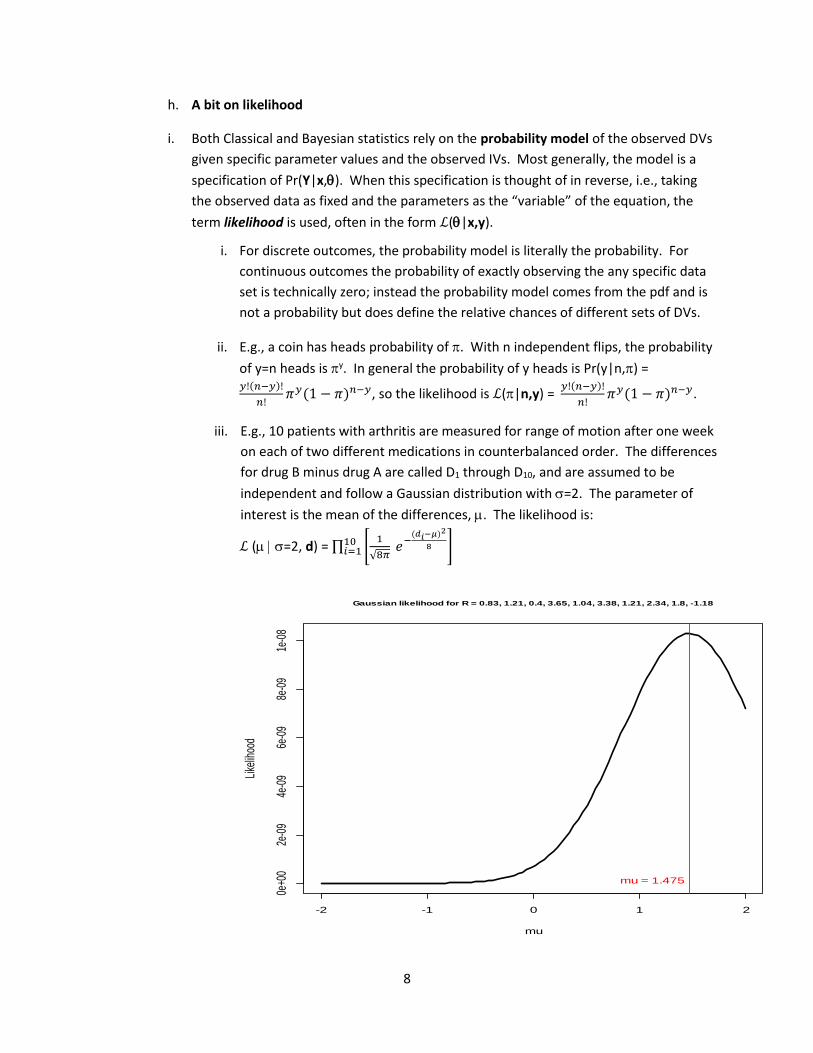
iii. E.g., 10 patients with arthritis are measured for range of motion after one week

on each of two different medications in counterbalanced order. The differences

for drug B minus drug A are called D1 through D10, and are assumed to be

independent and follow a Gaussian distribution with =2. The parameter of

interest is the mean of the differences, . The likelihood is:

ℒ (=2, d) = ∏ [1

√8𝜋 𝑒−

(𝑑𝑖−𝜇)2

8 ]10𝑖=1

-2 -1 0 1 2

0e+0

02e

-09

4e-0

96e

-09

8e-0

91e

-08

mu

Like

lihoo

d

Gaussian likelihood for R = 0.83, 1.21, 0.4, 3.65, 1.04, 3.38, 1.21, 2.34, 1.8, -1.18

mu = 1.475

9

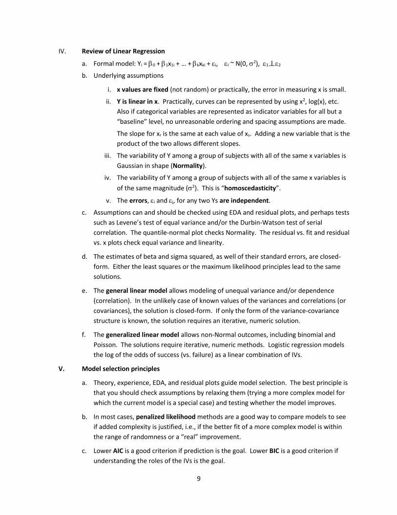
IV. Review of Linear Regression

a. Formal model: Yi = 0 + 1x1i + … + kxki + i, I ~ N(0, 2), 1 2

b. Underlying assumptions

i. x values are fixed (not random) or practically, the error in measuring x is small.

ii. Y is linear in x. Practically, curves can be represented by using x2, log(x), etc.

Also if categorical variables are represented as indicator variables for all but a

“baseline” level, no unreasonable ordering and spacing assumptions are made.

The slope for xr is the same at each value of xs. Adding a new variable that is the

product of the two allows different slopes.

iii. The variability of Y among a group of subjects with all of the same x variables is

Gaussian in shape (Normality).

iv. The variability of Y among a group of subjects with all of the same x variables is

of the same magnitude (2). This is “homoscedasticity”.

v. The errors, i and j, for any two Ys are independent.

c. Assumptions can and should be checked using EDA and residual plots, and perhaps tests

such as Levene’s test of equal variance and/or the Durbin-Watson test of serial

correlation. The quantile-normal plot checks Normality. The residual vs. fit and residual

vs. x plots check equal variance and linearity.

d. The estimates of beta and sigma squared, as well of their standard errors, are closed-

form. Either the least squares or the maximum likelihood principles lead to the same

solutions.

e. The general linear model allows modeling of unequal variance and/or dependence

(correlation). In the unlikely case of known values of the variances and correlations (or

covariances), the solution is closed-form. If only the form of the variance-covariance

structure is known, the solution requires an iterative, numeric solution.

f. The generalized linear model allows non-Normal outcomes, including binomial and

Poisson. The solutions require iterative, numeric methods. Logistic regression models

the log of the odds of success (vs. failure) as a linear combination of IVs.

V. Model selection principles

a. Theory, experience, EDA, and residual plots guide model selection. The best principle is

that you should check assumptions by relaxing them (trying a more complex model for

which the current model is a special case) and testing whether the model improves.

b. In most cases, penalized likelihood methods are a good way to compare models to see

if added complexity is justified, i.e., if the better fit of a more complex model is within

the range of randomness or a “real” improvement.

c. Lower AIC is a good criterion if prediction is the goal. Lower BIC is a good criterion if

understanding the roles of the IVs is the goal.

10

VI. Classical vs. Bayesian Inference

a. Fundamentals of classical inference

i. Parameters are considered to be fixed, unknown values.

ii. Inference is indirect: Consider the possible outcomes for a particular parameter

value and compare these to the observed outcomes.

iii. Real-life data is a subset (ideally random) from a population of outcomes.

Interest is in the population parameters, not the sample.

iv. Definition: a statistic is any quantity calculable from collected data (and known

constants) without using the (unknown) values of the parameters.

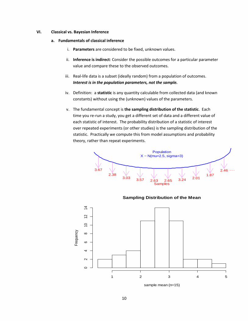
v. The fundamental concept is the sampling distribution of the statistic. Each

time you re-run a study, you get a different set of data and a different value of

each statistic of interest. The probability distribution of a statistic of interest

over repeated experiments (or other studies) is the sampling distribution of the

statistic. Practically we compute this from model assumptions and probability

theory, rather than repeat experiments.

Sampling Distribution of the Mean

sample mean (n=15)

Fre

qu

en

cy

1 2 3 4 5

02

46

81

01

21

4

Population

X ~ N(mu=2.5, sigma=3)

3.67

2.383.03

3.57 2.63 2.65 3.242.01

1.87

2.46 . . .

Samples

11

vi. The p-value for a given null hypothesis, e.g., H0: =0, is the probability of

obtaining the observed value of a given statistic or one less supportive of the

null hypothesis, based on the sampling distribution of that statistic under (i.e.,

assuming) that null hypothesis. A “small” p-value (less than , often using

=0.05) indirectly supports rejection of the null hypothesis because it says that

the observed data are unlikely given that the null hypothesis is true and that the

sampling distribution assumptions are true.

vii. Read carefully: Given that the null hypothesis is true and an appropriate

statistic and sampling distribution are used, the probability of the event

“p≤0.05” is 0.05 (5%). This is the type-1 (false positive) error rate. Because it is

not generally true that Pr(A|B)=Pr(B|A), we cannot make any probability

statement about the chance that H0 is true or false given p≤0.05!!!

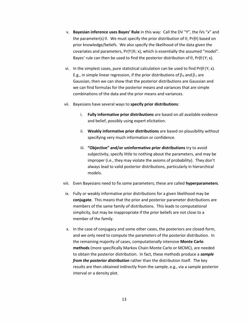
viii. Power is a key issue because when H0 is false, the observed statistic may not be

unlikely under H0. If the power of an experiment is high, then even under

“small” alternative hypotheses, the overlap between the null sampling

distribution of the test statistic and the alternative sampling distribution is

small, and only then do large p-values correspond to “the null hypothesis is

unlikely” (and the confidence intervals for the parameter are narrow).

ix. A 95% confidence interval (or other %) is a random interval for which we

expect over repeated studies the true parameter value will be contained inside

the interval 95% of the time. Again, this is a statement about the distribution of

the interval given a particular value of the parameter, and we cannot compute

the reverse; in fact, in classical statistics, the distribution of the parameter given

the interval does not make sense because the parameter is a fixed constant.

-2 0 2 4 6 8

0.0

0.2

0.4

0.6

0.8

1.0

Power: Null vs. Alternatives

Test Statistic

Dens

ity

p 0.05Null Sampling Distribution

Low Power Alternative

High Power Alternative

Null 0.05 Cutoff

12

x. The Multiple Comparison Problem: If multiple null hypotheses are true and you

do standard testing, the chance of a false positive (p≤0.05) grows very rapidly

with the number of tests. E.g., for 20 outcomes not related to treatment, the

chance of all p values being >0.05 is 1 – 0.9520 = 0.64, so there is a 36% chance

of at least one false positive. You have lost the protection of “only” 5% false

positives. Several good methods can be used to restore the type 1 error rate,

but all reduce power by a substantial degree. There is no free lunch!

b. Fundamentals of Bayesian inference

i. Bayesians consider parameters to have distributions which reflect our (perhaps

subjective) view as to what values are most likely.

ii. Bayesians are required to specify prior parameter distributions which reflect

their beliefs about the parameter values before observing their data.

iii. The main outcomes of a Bayesian analysis are posterior parameter

distributions which reflect what a rational observer should believe about the

parameter values after observing the data based on the standard laws of

probability adhered to by all statisticians and on the prior distributions.

Posterior probability intervals for parameters, the Bayesian parallel to Classical

confidence intervals, do behave like most naïve users incorrectly think

confidence intervals behave: if we compute a 95% posterior interval for , there

is a 95% chance that is inside the interval.

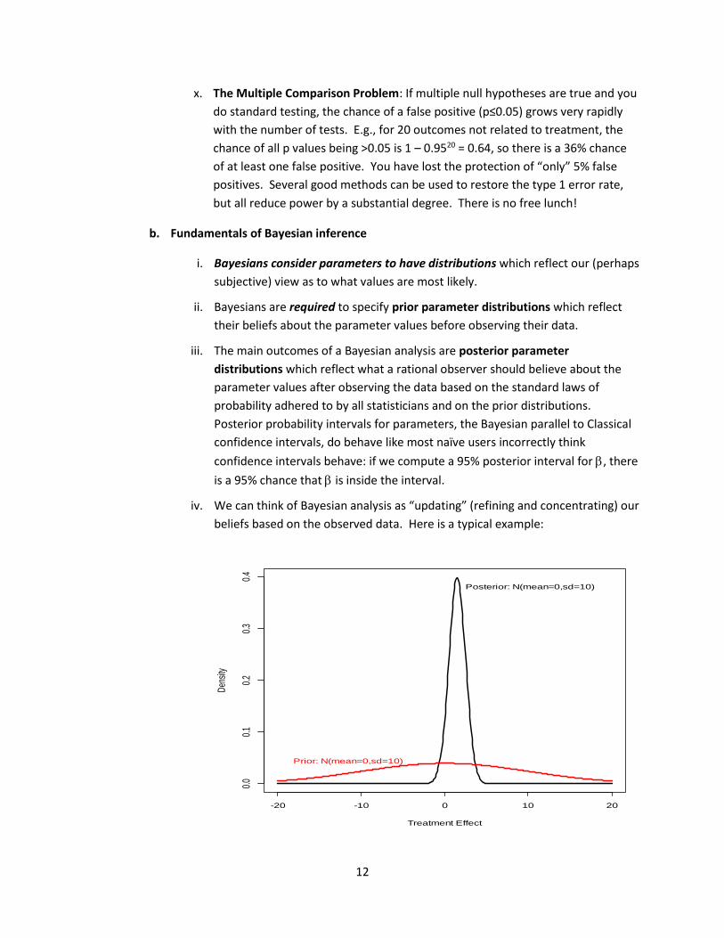
iv. We can think of Bayesian analysis as “updating” (refining and concentrating) our

beliefs based on the observed data. Here is a typical example:

-20 -10 0 10 20

0.0

0.1

0.2

0.3

0.4

Treatment Effect

Den

sity

Prior: N(mean=0,sd=10)

Posterior: N(mean=0,sd=10)

13

v. Bayesian inference uses Bayes’ Rule in this way: Call the DV “Y”, the IVs “x” and

the parameter(s) . We must specify the prior distribution of , Pr() based on

prior knowledge/beliefs. We also specify the likelihood of the data given the

covariates and parameters, Pr(Y|; x), which is essentially the assumed “model”.

Bayes’ rule can then be used to find the posterior distribution of , Pr(|Y; x).

vi. In the simplest cases, pure statistical calculation can be used to find Pr(|Y; x).

E.g., in simple linear regression, if the prior distributions of 0 and 1 are

Gaussian, then we can show that the posterior distributions are Gaussian and

we can find formulas for the posterior means and variances that are simple

combinations of the data and the prior means and variances.

vii. Bayesians have several ways to specify prior distributions:

i. Fully informative prior distributions are based on all available evidence

and belief, possibly using expert elicitation.

ii. Weakly informative prior distributions are based on plausibility without

specifying very much information or confidence.

iii. “Objective” and/or uninformative prior distributions try to avoid

subjectivity, specify little to nothing about the parameters, and may be

improper (i.e., they may violate the axioms of probability). They don’t

always lead to valid posterior distributions, particularly in hierarchical

models.

viii. Even Bayesians need to fix some parameters; these are called hyperparameters.

ix. Fully or weakly informative prior distributions for a given likelihood may be

conjugate. This means that the prior and posterior parameter distributions are

members of the same family of distributions. This leads to computational

simplicity, but may be inappropriate if the prior beliefs are not close to a

member of the family.

x. In the case of conjugacy and some other cases, the posteriors are closed-form,

and we only need to compute the parameters of the posterior distribution. In

the remaining majority of cases, computationally intensive Monte Carlo

methods (more specifically Markov Chain Monte Carlo or MCMC), are needed

to obtain the posterior distribution. In fact, these methods produce a sample

from the posterior distribution rather than the distribution itself. The key

results are then obtained indirectly from the sample, e.g., via a sample posterior

interval or a density plot.

14

xi. ҉ One of the beauties of Bayesian analysis is that it is relatively easy to

construct a computer algorithm to produce a sample of all of the parameters

from a complex model, even one that has never before been specified.

i. The Gibbs Sampling method allows one to compute each parameter in

turn rather than “jointly”.

ii. The Metropolis-Hastings algorithm is a general purpose method to

sample non-conjugate posterior distributions

xii. Available general purpose Bayesian software includes WinBUGS and jags. Both

may be run from within R. I use my R package, rube, to make the process

easier, safer, and more productive.

xiii. The information needed (by WinBUGS, jags, or for writing your own MCMC) is

the prior distributions and parameters and the directed acyclic graph (DAG). A

DAG is an intuitive method for specifying statistical models. Directed arrows

represent dependence relationships.

xiv. E.g., we think that our outcomes, Yi, are normally distributed with population

means, 0 + 1 *xi and with variance 2. We specify weakly informative prior

distributions as 0 ~ N(=0, =10), 1 ~ N(=0, =10), 2 ~ Gamma(=1,

=0.2). Here is the DAG:

15

VII. Single Level vs. Hierarchical Models

a. In studies with independent errors (deviations of the DVs from their mean given the IVs)

the likelihood for all of the DVs is the likelihood of each DV multiplied together. If the

errors are correlated, more complex models and corresponding likelihoods are needed,

which include correlation parameters rather than assuming zero correlation.

b. The means model states the population mean of the DV values for each

subject/treatment combination given the IVs and the parameter. The error model

specifies how the DV varies around that mean for different subject/treatment

combinations. If knowing the error (deviation from the mean) for one DV value changes

your knowledge about the error for another DV value, then these errors are correlated

and a model ignoring the correlation will result in using the wrong null sampling

distribution. Then everything based on the null sampling distribution will be wrong, e.g.

i. The p-value no longer tells the probability of obtaining the observed test

statistic or one more like the alternative under the null hypothesis. Specifically,

over repeated null studies p≤0.05 happens more frequently (anti-conservative)

or less frequently (conservative) than 5 % of the time.

ii. Confidence intervals are two wide or narrow.

iii. Power calculations are incorrect.

Similar problems occur in Bayesian analysis for other reasons.

c. The main sources of correlated DVs are

i. adjacency effects (temporal or spatial), e.g., stock prices or social networks

ii. hidden grouping where a part of the deviation from the mean for a group is due

to common, effective, unmeasured factors or covariates.

d. Hierarchies often lead to important hidden groupings

i. Students in the same classroom perform better or worse due to teacher (and

other classroom effects).

ii. Students in the same school perform better or worse due to administrative,

fiscal, cultural (and other school effects).

iii. Etc.

e. Appropriate modeling of correlation due to these hidden factors results in correct p-

values, confidence intervals, posterior distributions, etc. The common effects within a

group may be modeled directly as shared mean shifts or indirectly as correlations.

16

f. When a level of a hierarchy has many groups it often makes sense to estimate only the

variance of the shared group effects rather than estimating each individual effect,

because

i. future effects may be different (e.g., regress towards the mean)

ii. interest often centers on other groups than those studied, e.g., teachers in

general rather than the specific teachers of our study

iii. more “information” is available to more efficiently estimate other parameters of

interest if it is not “wasted” estimating the individual group effects

This idea of estimating only the variance (and subsequent induced correlation) for

effects whose levels are randomly chosen from a large population of effects is the main

idea behind random effects. In combination with the usual fixed effects, this gives

mixed effects models, a key tool in modeling hierarchical data.