pixel-based image classification
TRANSCRIPT
Pixel-based image classification
Lecture 7March 4, 2005

What is image classification or pattern recognition
Is a process of classifying multispectral (hyperspectral) images into patterns of varying gray or assigned colors that represent either
clusters of statistically different sets of multiband data, some of which can be correlated with separable classes/features/materials. This is the result of Unsupervised Classification, or numerical discriminators composed of these sets of data that have been grouped and specified by associating each with a particular class, etc. whose identity is known independently and which has representative areas (training sites) within the image where that class is located. This is the result of Supervised Classification.
Spectral classesSpectral classes are those that are inherent in the remote sensor data and are those that are inherent in the remote sensor data and must be identified and then labeled by the analyst.must be identified and then labeled by the analyst.
Information classesInformation classes are those that human beings define. are those that human beings define.

unsupervised classification, The computer or algorithm automatically group pixels with similar spectral characteristics (means, standard deviations, covariance matrices, correlation matrices, etc.) into unique clusters according to some statistically determined criteria. The analyst then re-labels and combines the spectral clusters into information classes.
supervised classification. Identify known a priori through a combination of fieldwork, map analysis, and personal experience as training sites; the spectral characteristics of these sites are used to train the classification algorithm for eventual land-cover mapping of the remainder of the image. Every pixel both within and outside the training sites is then evaluated and assigned to the class of which it has the highest likelihood of being a member.
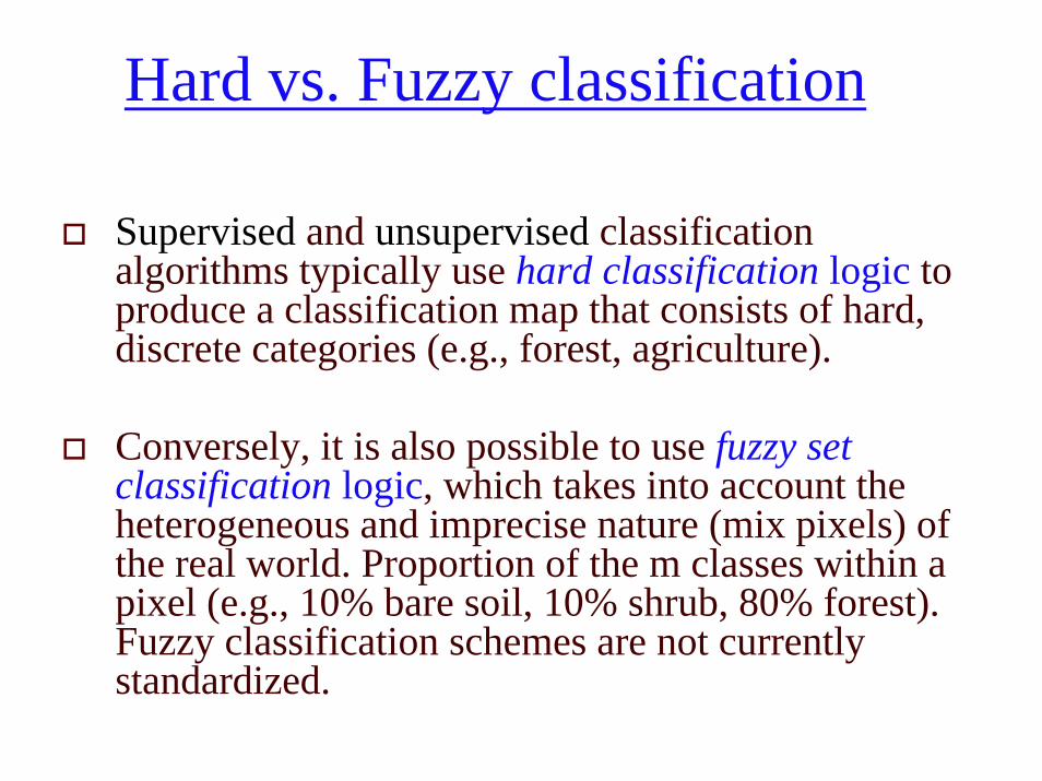
Hard vs. Fuzzy classification
Supervised and unsupervised classification algorithms typically use hard classification logic to produce a classification map that consists of hard, discrete categories (e.g., forest, agriculture).
Conversely, it is also possible to use fuzzy set classification logic, which takes into account the heterogeneous and imprecise nature (mix pixels) of the real world. Proportion of the m classes within a pixel (e.g., 10% bare soil, 10% shrub, 80% forest). Fuzzy classification schemes are not currently standardized.


Pixel-based vs. Object-oriented classification
In the past, most digital image classification was based on processing the entire scene pixel by pixel. This is commonly referred to as per-pixel (pixel-based) classification.
Object-oriented classification techniques allow the analyst to decompose the scene into many relatively homogenous image objects (referred to as patches or segments) using a multi-resolution image segmentation process. The various statistical characteristics of these homogeneous image objects in the scene are then subjected to traditional statistical or fuzzy logic classification. Object-oriented classification based on image segmentation is often used for the analysis of high-spatial-resolution imagery (e.g., 1 × 1 m Space Imaging IKONOS and 0.61 × 0.61 m Digital Globe QuickBird).

Knowledge-based information extraction: Artificial Intelligence
Neural networkDecision treeSupport vector machine (SVM)…

Purposes of classification
Land use and land cover (LULC)Vegetation typesGeologic terrainsMineral explorationAlteration mapping…….
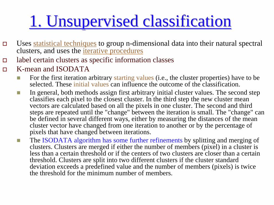
1. Unsupervised classification1. Unsupervised classificationUses statistical techniques to group n-dimensional data into their natural spectral clusters, and uses the iterative procedureslabel certain clusters as specific information classesK-mean and ISODATA
For the first iteration arbitrary starting values (i.e., the cluster properties) have to be selected. These initial values can influence the outcome of the classification.In general, both methods assign first arbitrary initial cluster values. The second step classifies each pixel to the closest cluster. In the third step the new cluster mean vectors are calculated based on all the pixels in one cluster. The second and third steps are repeated until the "change" between the iteration is small. The "change" can be defined in several different ways, either by measuring the distances of the mean cluster vector have changed from one iteration to another or by the percentage of pixels that have changed between iterations. The ISODATA algorithm has some further refinements by splitting and merging of clusters. Clusters are merged if either the number of members (pixel) in a cluster is less than a certain threshold or if the centers of two clusters are closer than a certain threshold. Clusters are split into two different clusters if the cluster standard deviation exceeds a predefined value and the number of members (pixels) is twice the threshold for the minimum number of members.


ISODATA: Initial Cluster Values (properties)
number of classes maximum iterationspixel change threshold (0 - 100%) (The change threshold is used to end the iterative process when the number of pixels in each class changes by less than the threshold. The classification will end when either this threshold is met or themaximum number of iterations has been reached)
initializing from statistics (Erdas) or from input (ENVI) (the initial values to put in for ENVI are minimum # pixel in class, maximum class stdv, minimum class distance, maximum # merge pairs)

5-10 classes, 8 iterations, 5 for change threshold, (MP 5, MSD 1, MD 5, MMP 2)


1-5 classes, 11 iterations, 5 for change threshold, (MP 5, MSD 1, MD 5, MMP 2)
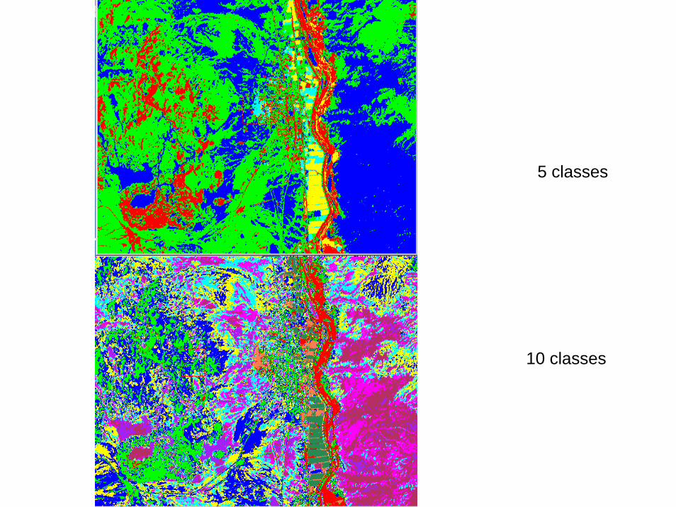
5 classes
10 classes

2. Supervised classification:training sites selection
Based on known a priori through a combination of fieldwork, map analysis, and personal experience
on-screen selection of polygonal training data (ROI), and/or
on-screen seeding of training data (ENVI does not have this, ErdasImagine does).
The seed program begins at a single x, y location and evaluates neighboring pixel values in all bands of interest. Using criteria specified by the analyst, the seed algorithm expands outward like an amoeba as long as it finds pixels with spectral characteristics similar to the original seed pixel. This is a very effective way of collecting homogeneous training information.
From spectral library of field measurements
Statistic extraction of each training site
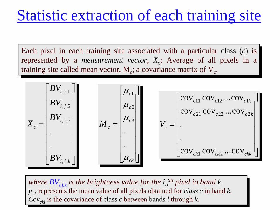
Each pixel in each training site associated with a particular class (c) is represented by a measurement vector, Xc; Average of all pixels in a training site called mean vector, Mc; a covariance matrix of Vc.
Each pixel in each training site associated with a particular class (c) is represented by a measurement vector, Xc; Average of all pixels in a training site called mean vector, Mc; a covariance matrix of Vc.
⎥⎥⎥⎥⎥⎥⎥⎥
⎦
⎤
⎢⎢⎢⎢⎢⎢⎢⎢
⎣
⎡
=
kji
ji
ji
ji
c
BV
BV
BV
BV
X
,,
3,,
2,,
1,,
.
.
⎥⎥⎥⎥⎥⎥⎥⎥
⎦
⎤
⎢⎢⎢⎢⎢⎢⎢⎢
⎣
⎡
=
ck
c
c
c
cM
µ
µµµ
.
.3
2
1
⎥⎥⎥⎥⎥⎥
⎦
⎤
⎢⎢⎢⎢⎢⎢
⎣
⎡
=
ckkckck
kccc
kccc
cV
cov...covcov..
cov...covcovcov...covcov
21
22221
11211
where BVi,j,k is the brightness value for the i,jth pixel in band k.µck represents the mean value of all pixels obtained for class c in band k. Covckl is the covariance of class c between bands l through k.
where BVi,j,k is the brightness value for the i,jth pixel in band k.µck represents the mean value of all pixels obtained for class c in band k. Covckl is the covariance of class c between bands l through k.

SelectingSelectingROIsROIs
Alfalfa
Cotton
Grass
Fallow

Spectra of ROIs from ETM+ image

Spectra from library
Resampled to matchTM/ETM+, 6 bands

Supervised classification methodsVarious supervised classification algorithms may be used to assign an unknown pixel to one of mpossible classes. The choice of a particular classifier or decision rule depends on the nature of the input data and the desired output. Parametric classification algorithms assumes that the observed measurement vectors Xc obtained for each class in each spectral band during the training phase of the supervised classification are Gaussian; that is, they are normally distributed. Nonparametricclassification algorithms make no such assumption.
Several widely adopted nonparametric classification algorithms include:one-dimensional density slicingparallepiped,minimum distance, nearest-neighbor, and neural network and expert system analysis.
The most widely adopted parametric classification algorithms is the:maximum likelihood.
Hyperspectral classification methodsBinary EncodingSpectral Angle MapperMatched FilteringSpectral Feature FittingLinear Spectral Unmixing

2.1 ParallepipedThis is a widely used digital image classification decision rule based on simple Boolean “and/or” logic.
ckckijkckck BV σµσµ +≤≤−
ckijkck HBVL ≤≤
If a pixel value lies above the low threshold and below the high threshold for all n bands being classified, it is assigned to that class. If the pixel value falls in multiple classes, ENVI assigns the pixel to the last class matched. Areas that do not fall within any of the parallelepipeds are designated as unclassified. In ENVI, you can use 1-3σ
Scann a table here p372
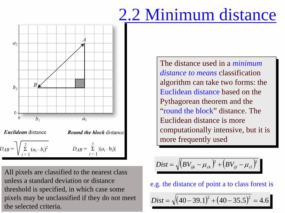
2.2 Minimum distance
( ) ( )22clijlckijk BVBVDist µµ −+−=
( ) ( )22clijlckijk BVBVDist µµ −+−=
The distance used in a minimum distance to means classification algorithm can take two forms: the Euclidean distance based on the Pythagorean theorem and the “round the block” distance. The Euclidean distance is more computationally intensive, but it is more frequently used
The distance used in a minimum distance to means classification algorithm can take two forms: the Euclidean distance based on the Pythagorean theorem and the “round the block” distance. The Euclidean distance is more computationally intensive, but it is more frequently used
( ) ( ) 6.45.35401.3940 22 =−+−=Dist
( ) ( )22clijlckijk BVBVDist µµ −+−=
All pixels are classified to the nearest class unless a standard deviation or distance threshold is specified, in which case some pixels may be unclassified if they do not meet the selected criteria.
e.g. the distance of point a to class forest is

2.3 Maximum likelihood
Instead based on training class multispectral distancemeasurements, the maximum likelihood decision rule is based on probability.The maximum likelihood procedure assumes that each training class in each band are normally distributed (Gaussian). Training data with bi- or n-modal histograms in a single band are not ideal. In such cases the individual modes probably represent unique classes that should be trained upon individually and labeled as separate training classes.the probability of a pixel belonging to each of a predefined set of m classes is calculated, and the pixel is then assigned to the class for which the probability is the highest. probability

The estimated probability density function for class wi (e.g., forest) is computed using the equation:
where exp [ ] is e (the base of the natural logarithms) raised to the computed power, xis one of the brightness values on the x-axis, is the estimated mean of all the values in the forest training class, and is the estimated variance of all the measurements in this class. Therefore, we need to store only the mean and variance of each training class (e.g., forest) to compute the probability function associated with any of the individual brightness values in it.
The estimated The estimated probability density functionprobability density function for class for class wwii (e.g., forest) is computed using (e.g., forest) is computed using the equation:the equation:
where where expexp [ ][ ] is is ee (the base of the natural logarithms) raised to the computed pow(the base of the natural logarithms) raised to the computed power, er, xxis one of the brightness values on the is one of the brightness values on the xx--axis, is the estimated mean of all the values axis, is the estimated mean of all the values in the forest training class, and is the estimated variancin the forest training class, and is the estimated variance of all the measurements in e of all the measurements in this class. this class. Therefore, we need to store only the mean and variance of each tTherefore, we need to store only the mean and variance of each training raining class (e.g., forest) to compute the probability function associaclass (e.g., forest) to compute the probability function associated with any of the ted with any of the individual brightness values in it.individual brightness values in it.
( )( )
( )⎥⎦
⎤⎢⎣
⎡ −−= 2
2
21 ˆ
ˆ21exp
ˆ2
1|ˆi
i
i
ixwxpσµ
σπ
iµ̂2ˆ iσ
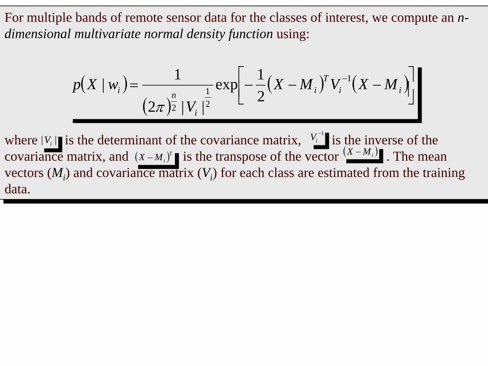
For multiple bands of remote sensor data for the classes of interest, we compute an n-dimensional multivariate normal density function using:
where is the determinant of the covariance matrix, is the inverse of the covariance matrix, and is the transpose of the vector . The mean vectors (Mi) and covariance matrix (Vi) for each class are estimated from the training data.
( )TiMX −
|| iV1−
iV( )iMX −
( )( )
( ) ( )⎥⎦⎤
⎢⎣⎡ −−−= −
iiT
i
i
ni MXVMXV
wXp 1
21
221exp
||2
1|π

If we assume that there are m classes, then p(X/wi) is the probability density function associated with the unknown measurement vector X, given that X is from a pattern in class wi. In this case the maximum likelihood decision rule becomes:Decide if, and only if,
for all i and j out of 1, 2, ... m possible classes.
Therefore, to classify a pixel in the multispectral remote sensing dataset with an unknown measurement vector X, a maximum likelihood decision rule computes the product for each class and assigns the pattern to the class having the largest product. This assumes that we have some useful information about the prior probabilities of each class i (i.e., p(wi)).
iwX ∈
( ) ( ) ( ) ( )jjii wpwXpwpwXp ⋅≥⋅ ||
Without Prior Probability InformationWithout Prior Probability Information::Decide unknown measurement vector Decide unknown measurement vector XX is in is in class class ii if, and only if,if, and only if,ppii >> ppjjfor allfor all ii andand j j out of 1, 2, ...out of 1, 2, ... mm possible classespossible classesandand
( ) ( )⎥⎦⎤
⎢⎣⎡ −−−= −
iiT
iiei MXVMXVp 1
21||log
21
Unless you select a probability threshold (0-1), all pixels are classified. Each pixel is assigned to the class that has the highest probability

2.4 Mahalanobis Distance
M-distance is similar to the Euclidian distance
( ) ( )iiT
i MXVMXDist −••−= −1
It is similar to the Maximum Likelihood classification but assumes all class covariances are equal and therefore is a faster method. All pixels are classified to the closest ROI class unless you specify a distance threshold, in which case some pixels may be unclassified if they do not meet the threshold (in DN number)

2.5 Spectral Angle Mapper

2.6 Spectral Feature Fitting
compare the fit of image spectra to selected reference spectra using a leastleast--squares techniquesquares technique. SFF is an absorption-feature-based methodology. The reference spectra are scaled to match the image spectra after continuum removal from both data sets. A scale image is output for each reference spectrum and is a measure of absorption feature depth which is related to material abundance. The image and reference spectra are compared at each selected wavelength in a least-squares sense and the root mean square (rms) error is determined for each reference spectrum.

Supervisedclassificationmethod:
Spectral FeatureFitting
Source: http://popo.jpl.nasa.gov/html/data.html

3. Application: LULC classification
Land cover refers to the type of material present on the landscape (e.g., water, sand, crops, forest, wetland, human-made materials such as asphalt).
Land use refers to what people do on the land surface (e.g., agriculture, commerce, settlement).
The pace, magnitude, and scale of human alterations of the Earth’s land surface are unprecedented in human history. Therefore, land-cover and land-use data are central to such United Nations’ Agenda 21 issues as combating deforestation, managing sustainable settlement growth, and protecting the quality and supply of water resources.

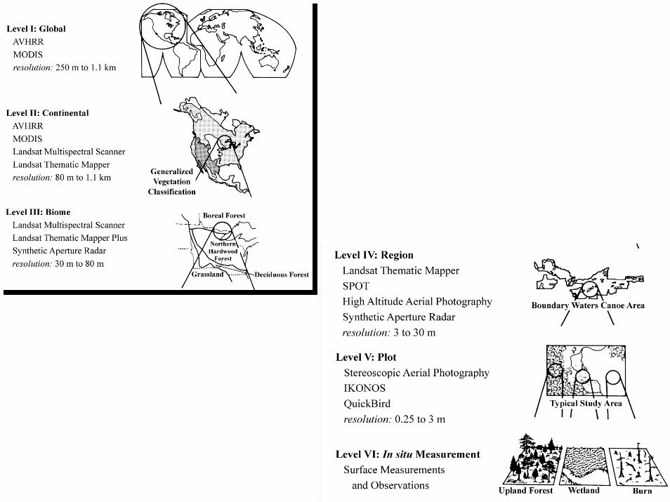
USGS LULC levels
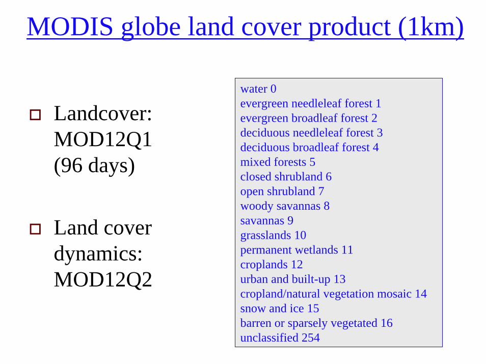
MODIS globe land cover product (1km)
water 0 evergreen needleleaf forest 1 evergreen broadleaf forest 2 deciduous needleleaf forest 3 deciduous broadleaf forest 4 mixed forests 5 closed shrubland 6 open shrubland 7 woody savannas 8 savannas 9 grasslands 10 permanent wetlands 11 croplands 12 urban and built-up 13 cropland/natural vegetation mosaic 14 snow and ice 15 barren or sparsely vegetated 16 unclassified 254
Landcover: MOD12Q1 (96 days)
Land cover dynamics: MOD12Q2