place-based preferential effects: evidence from · pdf filefor attribution, translations,...
TRANSCRIPT

ASIAN DEVELOPMENT BANK
AsiAn Development BAnk6 ADB Avenue, Mandaluyong City1550 Metro Manila, Philippineswww.adb.org
Place-Based Preferential Tax Policy and Its Spatial Effects: Evidence from India’s Program on Industrially Backward Districts
Place-based policies aimed at enhancing economic performance of certain areas within a country or region have been popular in developed and developing countries. These policies often involve tax exemptions, subsidies, discretionary grants, special economic zones, and/or infrastructure support. This paper studies a typical preferential tax program that the Government of India initiated in 1994 which targeted 123 industrially backward districts in 14 states.
Using a regression discontinuity design to evaluate the program’s impacts, the study finds that the program led to a significant increase in firm entry and employment among light manufacturing industries in betteroff backward districts. However, the program also resulted in considerable negative spillovers in adjacent districts that were weaker in economic activity.
About the Asian Development Bank
ADB’s vision is an Asia and Pacific region free of poverty. Its mission is to help its developing member countries reduce poverty and improve the quality of life of their people. Despite the region’s many successes, it remains home to a large share of the world’s poor. ADB is committed to reducing poverty through inclusive economic growth, environmentally sustainable growth, and regional integration.
Based in Manila, ADB is owned by 67 members, including 48 from the region. Its main instruments for helping its developing member countries are policy dialogue, loans, equity investments, guarantees, grants, and technical assistance.
adb economicsworking paper series
NO. 524
november 2017
PlAcE-BASED PrEfErENTIAl TAx POlIcy AND ITS SPATIAl EffEcTS: EvIDENcE frOm INDIA’S PrOgrAm ON INDuSTrIAlly BAckwArD DISTrIcTSRana Hasan, Yi Jiang, and Radine Michelle Rafols

ADB Economics Working Paper Series
Place-Based Preferential Tax Policy and Its Spatial Effects: Evidence from India’s Program on Industrially Backward Districts Rana Hasan, Yi Jiang, and Radine Michelle Rafols
No. 524 | November 2017
Rana Hasan ([email protected]) is a director, Yi Jiang ([email protected]) is a senior economist, Radine Michelle Rafols ([email protected]) is a consultant at the Economic Research and Regional Cooperation Department, Asian Development Bank. The authors are grateful to Giles Duranton for very useful suggestions.

Creative Commons Attribution 3.0 IGO license (CC BY 3.0 IGO)
© 2017 Asian Development Bank6 ADB Avenue, Mandaluyong City, 1550 Metro Manila, PhilippinesTel +63 2 632 4444; Fax +63 2 636 2444www.adb.org
Some rights reserved. Published in 2017.
ISSN 2313-6537 (Print), 2313-6545 (electronic)Publication Stock No. WPS179107-2DOI: http://dx.doi.org/10.22617/ WPS179107-2
The views expressed in this publication are those of the authors and do not necessarily reflect the views and policies of the Asian Development Bank (ADB) or its Board of Governors or the governments they represent.
ADB does not guarantee the accuracy of the data included in this publication and accepts no responsibility for any consequence of their use. The mention of specific companies or products of manufacturers does not imply that they are endorsed or recommended by ADB in preference to others of a similar nature that are not mentioned.
By making any designation of or reference to a particular territory or geographic area, or by using the term “country” in this document, ADB does not intend to make any judgments as to the legal or other status of any territory or area.
This work is available under the Creative Commons Attribution 3.0 IGO license (CC BY 3.0 IGO) https://creativecommons.org/licenses/by/3.0/igo/. By using the content of this publication, you agree to be bound by the terms of this license. For attribution, translations, adaptations, and permissions, please read the provisions and terms of use at https://www.adb.org/terms-use#openaccess
This CC license does not apply to non-ADB copyright materials in this publication. If the material is attributed to another source, please contact the copyright owner or publisher of that source for permission to reproduce it. ADB cannot be held liable for any claims that arise as a result of your use of the material.
Please contact [email protected] if you have questions or comments with respect to content, or if you wish to obtain copyright permission for your intended use that does not fall within these terms, or for permission to use the ADB logo.
Notes:1. In this publication, “$” refers to US dollars.2. Corrigenda to ADB publications may be found at http://www.adb.org/publications/corrigenda

CONTENTS TABLES AND FIGURE iv ABSTRACT v I. INTRODUCTION 1 II. POLICY BACKGROUND 4 III. EMPIRICAL STRATEGY 7 IV. DATA 11 V. RESULTS 13 A. Program Impacts on the Backward Districts 13 B. Spatial Effects of the Program 21 C. Robustness Checks 26 VI. CONCLUSION 26 APPENDIXES 29 REFERENCES 35

TABLES AND FIGURE TABLES 1 State-Wise Distribution of Backward and Nonbackward Districts 6 2a T-tests of Pretreatment District Variables in 1991 8 2b T-tests of District Pretreatment Variables in 1991 After Controlling for 3rd Order Polynomial of Gradation Scores 9 3 Summary Statistics of Number of Firms and Employment by District Groups and Industrial Category 13 4a Program Impacts on Number of Firms at 2-Digit Industry by District Level 16 4b Program Impacts on Employment at 2-Digit Industry by District Level 17 5 Program Impacts at 2-Digit Industry–District Level: Distinguishing Light versus Heavy
Manufacturing 20 6 Number and Average Gradation Scores by Neighboring Districts 22 7 Spatial Effects of the Program 24 A1 Indicators Used to Construct Gradation Scores to Identify Backward Districts 29 A2 Program Impacts on Firm Count At 2-Digit Industry–District Level (Dependent Variable Log-Transformed) 30 A3 Program Impacts on Employment at 2-Digit Industry–District Level (Dependent Variable Log-Transformed) 31 A4 Program Impacts at 2-Digit Industry–District Level: Distinguishing Light versus Heavy
Manufacturing (Dependent Variables Log-Transformed) 32 A5 Spatial Effects of the Program (Dependent Variables Log-Transformed) 33 FIGURE 1 Mean Counts of Firms and Employment of 2-Digit Industry by District Relative to the Gradation Scores 14

ABSTRACT The Government of India initiated a program in 1994 to promote manufacturing in districts designated as backward. The way the backward districts were identified enables us to employ a regression discontinuity design to evaluate the impacts of the program. We find that the program’s 5-year tax exemption to manufacturers led to a significant increase in firm entry and employment in relatively better-off backward districts, particularly in light manufacturing industries. However, the program also resulted in negative spillover effects in districts which were neighboring these backward districts and relatively weaker in economic activity. The findings emphasize that the spatial effects of place-based policies deserve greater attention from policy makers. Keywords: backward districts, place-based policy, preferential tax, sharp regression discontinuity, spatial spillovers JEL codes: H32, O14, R12
I. INTRODUCTION Place-based policies aimed at enhancing economic performance of certain areas within a country or region have been popular in both developed and developing countries. Examples of large-scale, place-based policies include the federal Empowerment Zone Program in the United States established in 1993, various initiatives of the European Union supported under its structural funds targeted at disadvantaged areas and countries within the European Union, and the special economic zones of the People’s Republic of China (PRC) that were started in the late 1970s, to name a few (see Neumark and Simpson 2015 for a detailed review).
A common goal of place-based policies is to create jobs and spur economic activity by attracting
new firms and/or promoting local firm growth in the selected underdeveloped areas. The policies usually take one or a combination of the following forms: tax exemptions and subsidies, discretionary grants, special economic zones or industrial parks, and infrastructure support. The policy studied in this paper is a typical preferential tax program the Government of India adopted in 1994 that targeted 123 backward districts in the country’s 14 major states.
Place-based policies are often designed in connection with another category of public policies
used by governments: industrial policies. For instance, special economic zones or industrial parks are often set up to promote certain industries such as high technology manufacturing. In the preferential tax program that we examined, the service sector as well as some manufacturing industries are not covered by the policy even if firms in these sectors are located in the backward districts.
Placed-based policies are likely to bear more economic and political significance in developing
countries as compared to developed countries. First, for a country at the early stage of development, placed-based policies could be used to enhance economic performance of the selected areas, which are then anticipated to lead the development of the whole country. One such case is the PRC’s experiment with special economic zones. Second, geographic disparities are arguably larger in developing countries. The weaker-performing areas of a developing country are often characterized by large populations and/or greater poverty incidence. Placed-based policies targeting these areas often have dual objectives of promoting economic development and reducing inequality. Third, the underdeveloped areas often account for a larger share of the population in a developing country. Policies favoring these areas are likely to win political support and considered important by politicians.
The interest in the impacts of a place-based policy is often twofold. First, does the policy benefit
the targeted areas as the policy makers expect? For a firm to locate in a particular place, it is possible that some basic conditions such as availability of basic infrastructure or human capital need to be met. Among several candidate places, the firm is likely to choose the optimal one based on an array of criteria while government policy may improve just one or some. Therefore, a preferential policy may not change the relative competitiveness of the targeted areas in attracting firms as much as expected. Second, what kind of spatial effects does the policy generate? On the one hand, a place-based policy may result in positive spillovers to areas neighboring the policy-treated areas. This can happen, for example, when increasing production and employment in the latter create more demand for inputs and services across geographic borders. On the other hand, given the mobility of labor and capital, the policy may produce considerable displacement effects in untreated neighboring areas, especially when treated and untreated areas are otherwise similar.
This paper attempts to address three interrelated questions regarding the backward districts
program. First, did the program lead to an increase in manufacturing firms and jobs in the targeted
2 | ADB Economics Working Paper Series No. 524
districts? Related to this, we also explore whether the program had different effects on light and heavy manufacturing industries and had any positive spillovers to other untreated sectors through production linkages and agglomeration effects. Second, did the program have any differential impacts on the targeted districts? As discussed above, the program that essentially lowers the production costs through offering tax exemptions may not boost the attractiveness of all targeted districts to new firms. If so, it is important to understand who actually benefits from such policies. Third, what are the net spatial effects generated by the program? How do they compare with the effects of the program on treated districts?
There are two challenges in addressing these questions. First, a key challenge of evaluating the
impact of placed-based policies lies in the fact that the targeted areas are not randomly selected in most cases. The untreated areas do not necessarily constitute good counterfactuals for the treated areas. The approach that the Government of India used to identify backward districts, however, offers us a unique opportunity to assess the program’s impact more credibly. In short, the government assigned a gradation score to each district from India’s 14 major states based on their historical indicators. The districts with scores below a cutoff point were designated backward districts and treated with the tax exemption policy (see next section for more detailed description). This setting allows us to use a (sharp) regression discontinuity design in estimating the causal effects of the program. Upon checking the pretreatment district covariates, we show that the score is a good proxy for districts’ demographic and development characteristics. Hence, the untreated districts with scores right above the cutoff point are a sound control group for the treated districts right below the cutoff. Regressions with samples of districts near the cutoff point should yield plausible estimates of the program’s effects. For estimating spatial effects, we again use the gradation scores. We compare districts from the same score group with and without any treated districts in their neighborhood while controlling for score groups of other neighboring districts.
Second, while the ideal data for capturing the effects of place-based policies are panel data that
capture the number of firms and employment levels by location and industry, such data are quite rare, especially for geographically focused locations such as a district.1 We get around this difficulty by using the extensive coverage of firms within and across districts captured by India’s 1998 economic census and use the regression discontinuity design noted above to infer the effects of the backward district program from the cross-sectional variation in firm and employee counts across districts.
Our main findings are as follows. First, by 1998 about one-third of the backward districts with
the gradation scores nearest to the cutoff had significantly more firms and employment (both more than 50%) in the light manufacturing industries. Firm and employment counts were also higher in heavy manufacturing industries, but insignificantly so. The policy also seems to have generated some agglomeration effects, possibly through input–output linkages, as reflected in moderately higher firm and employment counts in the untreated sectors including construction, mining, and services in these districts.
Second, when we expand the estimation samples from those near the cutoff to all districts, the
point estimates are weakened or change signs, implying that the above positive effects were concentrated in the treated districts with relatively higher gradation scores. This suggests that preferential tax treatment alone is unlikely to be a sufficient condition for firm entry and employment
1 Thus, while the Annual Survey of Industry and National Sample Survey Organization’s surveys of unregistered enterprises
are one potential source of information on the number of enterprises and employment by industry, they are sample surveys for the most part and may not capture accurately the number of firms and employment levels at the district level.
Place-Based Preferential Tax Policy and Its Spatial Effects | 3
growth in the more challenged areas. Basic infrastructure, human capital, and access to credit may be necessary for agglomerations to take effect in those areas.
With respect to the spatial effects of the program, our findings strongly suggest that the
characteristics of both treated districts and their neighbors matter. For districts from the lower-ranked treated groups or from the untreated group right above the cutoff point, those with at least one neighboring district from the treated group right below the cutoff point had considerably fewer firms and smaller employment as opposed to those without any neighboring district from that group. However, for districts far above the cutoff, there is no difference in whether or not they have such a neighboring district. Furthermore, a neighboring district from a lower-ranked treated group or from any untreated group does not have much impact on its neighbors. The results suggest that the program generated acute spatial competition mainly between relatively better-off program-targeted districts and their neighbors with weak capacity. The latter, even if also favored by the program, seem to have lost employment to the former due to firm relocation. The displacement effects are quite significant and largely offset the positive impacts of the program on the treated districts. It is hard, however, for the better-off treated districts to attract firms from those districts which are economically stronger. It is also difficult for the worse-off treated districts to lure firms from their neighbors.
This paper contributes to a growing literature on place-based policies in the following ways.2
Evidence on the effects of economic and/or enterprise zones in creating jobs, mainly from the developed countries so far, are generally mixed. For instance, Neumark and Kolko (2010) found that the California Enterprise Zones program had no significant effects in generating employment while Hanson (2009) noted the same with the Federal Empowerment Zones program, whereas Freedman (2013) found positive effects for the Texas Enterprise Zones program as did Busso, Gregory, and Kline (2013) for the Federal Empowerment Zones program. As far as spillovers are concerned, Givord, Rathelot, and Sillard (2013) found strong displacement effects of the French Zones Franches Urbaines (ZFUs) program on the nearby non-ZFU areas, which were of comparable magnitude to the positive effects the program generated inside the ZFUs. However, the results for the United States programs are mixed again. We add to this literature by showing that the tax exemption policy has differential impacts depending on the characteristics of the receiving areas with positive effects on firm entry and employment growth concentrated in the relatively well-performing targeted areas. We also show that strong displacement effects exist mainly between the better-off treated areas and their relatively weak neighbors which are either treated or not.
Although place-based policies have been adopted prominently by developing country
governments, evidence about their impacts is still limited. Studying the impact of the special economic zones program in the PRC, Wang (2013) found that these zones increased the level of foreign direct investment and exports as well as average wages of workers in the host municipalities and generated a moderate displacement effect in the adjacent municipalities. Closer to our paper is Chaurey (2016), which examines the New Industrial Policy of India’s federal government that offered tax exemptions and capital subsidies for firms in two states, Uttarakhand and Himachal Pradesh, since 2003. Applying a difference-in-differences approach, the author showed that the policy resulted in large increases in outcomes such as employment, number of firms, and total output in the treatment states relative to the control states. In addition, he did not find relocation of firms underlying the impact of the policy.
Apart from similarities in policy content, the backward district program studied here differs from
the New Industrial Policy along several dimensions. For instance, the program covered 14 major states 2 See Neumark and Simpson (2015) for a comprehensive survey of the literature.
4 | ADB Economics Working Paper Series No. 524
of India, which are more populated and many of which are economically advanced as compared to Uttarakhand and Himachal Pradesh. The program was administered at the district level with selection of the treated areas based on some predetermined scores. These unique features enable us to implement a distinctive identification strategy and examine the program’s impact at a finer geographic level. Moreover, our findings about the differential impacts on the treated districts and the conditional displacement effects could offer an explanation of the distinct results of the two studies with respect to the spatial effects.
This paper is also connected with the literature on the location and growth of firms in response
to local taxation. The available evidence is somewhat mixed. Some studies, e.g., Rathelot and Sillard (2008) find a weak response of firms’ location choice to higher taxes, while others, e.g., Bartik (1991) and Guimaraes, Figueiredo, and Woodward (2004), find a negative relationship. After correcting potential endogeneity issues, Duranton, Gobillon, and Overman (2011) find that local taxation has a negative impact on firm employment but no effect on firm entry in the United Kingdom. Our results suggest that the taxation impacts may depend on the local characteristics, which enter firms’ decision functions as well.
The rest of the paper is organized as follows. Section II introduces the background and key
aspects of the backward district program. Section III discusses the empirical strategy for estimating the effects of the program, and section IV describes the data. Section V presents the results, and section VI concludes with some discussions on the policy implications.
II. POLICY BACKGROUND Like many developing countries, the spatial pattern of economic activity in India is characterized by a concentration of industrial development around large cities and development skewed toward a few states. Analysis shows the coefficient of variation of per state domestic product had risen from 25% in 1950–1951 to 35% in 1993–1994 (Ghosh et al. 1998). In response, the Government of India has implemented various policies and programs to reduce regional imbalance and inequality since India’s independence in 1947. We provide a brief review of the evolution of these policies before introducing the program evaluated in this paper.
India’s approach to balancing regional development can be distinguished into three phases: a
first phase spanning 1948–1980, then a period of nascent market-oriented reforms in the 1980s, and finally a postreform era commencing right after the dramatic trade and industrial policy reforms of 1991. The initial years of planning were characterized by heavy public sector involvement and direct central intervention to minimize spatial divergence (Singhi 2012). Several policy tools pursued in this period included (i) industrial licensing, (ii) direct investment in public sector units, and (iii) price controls and distribution policies to equalize access to production inputs and negate locational advantages. While investment and transport subsidies were awarded to industries set up in backward areas, restrictions were imposed on private enterprises to discourage concentration in well-developed states.3 In the mid-1960s and 1970s, the scope of such policies were further widened to include infrastructure support, fiscal incentives, and concessions (Planning Commission 1961, 1966). However, despite these sustained efforts, regional disparities continued to persist and industrial development remained concentrated around large cities (Ghosh et al. 1998; MCI 1977).
3 Depending on the policy intervention, backward areas may refer to underperformed states, districts, zones, or rural areas.
Place-Based Preferential Tax Policy and Its Spatial Effects | 5
At the onset of the early reform period, several studies and policy makers expressed concern about the interventionist strategy pursued. Programs were criticized for having little understanding of the needs and weaknesses of local areas (Planning Commission 1981a; Aggarwal and Archa 2013). In 1981, the National Committee on the Development of Backward Areas found subsidies and concessional finance to be insignificant factors in motivating firms to locate their industrial units in disadvantaged areas (Planning Commission 1981b). Against the backdrop of political decentralization and a liberalizing global economy, the government eliminated many of the controls earlier exercised by the central government. The Industrial Policy Statement of 1991 announced major changes to the government’s role, reducing industrial licensing, relaxing industrial location policy, and allowing entry of large enterprises into small-scale industry sector (e.g., see Martin, Nataraj, and Harrison 2017; MCI 1991). Focus shifted from a centrally planned top–down strategy toward nationwide fiscal discipline and sustainable incentive structures that encouraged private-sector-driven growth (Saikia 2009).
Despite the paradigm shift toward local planning in the postreform era, a study conducted by
the National Institute of Public Finance and Policy in 1987 suggested enlargement of central government tax incentives in the Income Tax Act to encourage entrepreneurship and industrial dispersal. Following this, the Finance Act of 1993 introduced a tax holiday scheme for new industrial undertakings4 located in backward states and union territories.5
Immediately after the introduction of the 1993 Act, the Ministry of Finance commissioned a
review to assess industrially challenged districts located in the remaining 14 states which were not designated backward. The Study Group on Fiscal Incentives adopted an index-based approach to select districts and proposed similar fiscal support to boost investment, industrialization, and job creation in these districts. Specifically, they developed a composite index based on eight financial, infrastructural, and industrial indicators to approximate a district’s degree of development. The individual scores on the indicators for each district are calculated as a percentage relative to India’s nationwide average. The overall score is the weighted sum of the eight individual scores with weights equal to 1, 2, or 3 (see Table A1 for details). We refer to the overall scores as “gradation scores” hereafter in that they were published in the “All India Gradation List” developed through the Finance Act of 1994 as Appendix III of the Income Tax Act.
Districts that had failed to score above 500 were accorded backward status, which qualified
them for the preferential tax treatment enacted by the Finance Act of 1994. Out of the total 360 districts from the 14 states, 120 had gradation scores below 500 and were designated industrially backward districts. Three additional districts were tagged as backward districts despite scoring above 500 due to nonscore-based characteristics including the district falling under the category of a "no industry" 6 district, or an inaccessible hill area district as indicated in the Eighth Plan Document, or if the district did not have a “railhead” as on 1 April 1994.7
4 Per section 3d of the Industries (Development and Regulation) Act of 1951, “industrial undertaking” pertains to a scheduled
industry carried on in one or more factories by any person or authority including the government. 5 These are states and union territories located in the northeastern and northwestern parts of India and on the islands. 6 The Government of India introduced the concept of “no industry” districts in March 1982. The Government of India also
introduced a scheme of assistance (basically to subsidize infrastructural development of the area) in April 1983. The “no industry” district is one where there is no industry requiring a capital investment in plant and machinery equal to or exceeding ₹10 million. In such a district, the “nucleus plant” or the “mother industry” attempts to create ancillary industries over a widely dispersed area, and thereby tries to create employment opportunities for local people.
7 The three districts are Idukki (618) and Wayanad (583) in Kerala and Jalapaiguri (728) in West Bengal. We do not include the three exceptions in our baseline analysis and show they have no influence on the results in our robustness checks.

6 | ADB Economics Working Paper Series No. 524
In our analysis, we divide all the districts into six groups from the most challenged to the most advanced based on the gradation scores and label them from 1 to 6, which are Group 1: <250, Group 2: 251–350, Group 3: 351–500, Group 4: 501–650, Group 5: 651–850, and Group 6: >850. As such, Groups 1–3 were the treated districts and 4–6 were not treated. Groups 3 and 4 are nearest the cutoff point, Groups 2 and 5 farther away, and so forth. Table 1 presents the state-wise distribution of backward and nonbackward districts by groups. Each group except the most advanced one has approximately the same number of districts. Eleven out of 14 states have both backward and nonbackward districts. Most districts in the three states, Haryana, Punjab, and Tamil Nadu, which do not have any backward districts, are in Group 6. Two states, Bihar and Uttar Pradesh, each host over a quarter of the backward districts, while another quarter were located in states Madhya Pradesh and Rajasthan.
Table 1: State-Wise Distribution of Backward and Nonbackward Districts
Backward Nonbackward
State Name Group
1 Group
2 Group
3 Total Group
4 Group
5 Group
6 Total Andhra Pradesh – – 2 2 – 9 12 21 Bihar 19 10 4 33 3 1 5 9 Gujarat – 2 1 3 – 1 15 16 Haryana – – – – – 1 15 16 Karnataka – – 1 1 3 4 12 19 Kerala 2 – – 2 1 2 9 12 Madhya Pradesh 3 7 8 18 10 5 12 27 Maharashtra 1 – 1 2 7 6 15 28 Orissa 2 2 2 6 3 1 3 7 Punjab – – – – – – 12 12 Rajasthan 2 6 4 12 4 3 8 15 Tamil Nadu – – – – 2 3 16 21 Uttar Pradesh 6 16 13 35 5 5 18 28 West Bengal 6 2 1 9 1 – 5 6 Total 41 44 38 123 39 41 157 237
Notes: Samples were subdivided into groups per gradation scores. Group 1 contains districts with scores equal or below 250; Group 2 from 251 to 350; Group 3 from 351 to 500; Group 4 from 501 to 650; Group 5 from 651 to 850; Group 6 850 and above. Groups 1–3 were treated and Groups 4–6 were untreated. Three districts with gradation scores exceeding 500 while tagged as category A backward districts, i.e., Idukki (618) and Wayanad (583) from Kerala and Jalapaiguri (728) from West Bengal, are included as Group 1 since category A is districts scoring 250 or lower. Source: Authors’ estimates.
The program, as stipulated in Section 80-IA of the Income Tax Act, offered new industrial
undertakings in the backward districts a tax holiday in which firms are granted tax deductions of 100% of profits and gains for the first 5 assessment years. After the initial 5 assessment years, deduction from the profits would be allowed at the normal rate of 30% in the case of companies and 25% in the case of noncorporate assessees. The deduction, at the enhanced rate and the normal rate together, was limited to 12 assessment years in the case of cooperative societies and 10 assessment years in the case of other assessees. To be eligible for the benefits, the industrial undertaking had to “begin to manufacture or produce articles or things or to operate its cold storage plant or plants at any time during the period beginning on the 1st day of October, 1994 and ending on the 31st day of March, 2000.” The program

Place-Based Preferential Tax Policy and Its Spatial Effects | 7
excluded a few industries or economic activities from receiving tax exemption such as manufacture of products of tobacco, alcohol spirits, confectionery, and aerated waters.8
The government further classified backward districts into categories A and B in September 1997.
Those belonging to category A had scores of 250 or lower, or had scores between 251 and 500 and one of the nonscore-based characteristics as noted above. The full tax deduction was extended for another 5 years for category A districts and 3 years for category B districts.
III. EMPIRICAL STRATEGY We evaluate the effects of the backward district program undertaken by the Government of India since October 1994 using the 1998 Economic Census to generate information on the number of firms and employment at the two-digit industry level and across districts. While the backward districts could be substantially different from the nonbackward districts on observables and nonobservables, the way the government used to identify the backward districts allows us to apply the (sharp) regression discontinuity design to estimating the program’s causal impact on the economic activity in the backward districts.
As described in the previous section, the districts were assigned a composite score in 1993 which
was computed based on 1991 census data. The treatment status was determined strictly on whether the score is above the cutoff point (500) or not. It is hard to conceive of any way through which a district could manipulate its score to make itself eligible for the program. Therefore, the variation in treatment status could be considered as good as randomized for districts in the neighborhood around the cutoff (Lee and Lemieuxa 2010). Thus, the regression discontinuity design offers an appropriate identification strategy to estimate the program’s impact.
To verify this assumption, we compare the pretreatment variables between the treated and
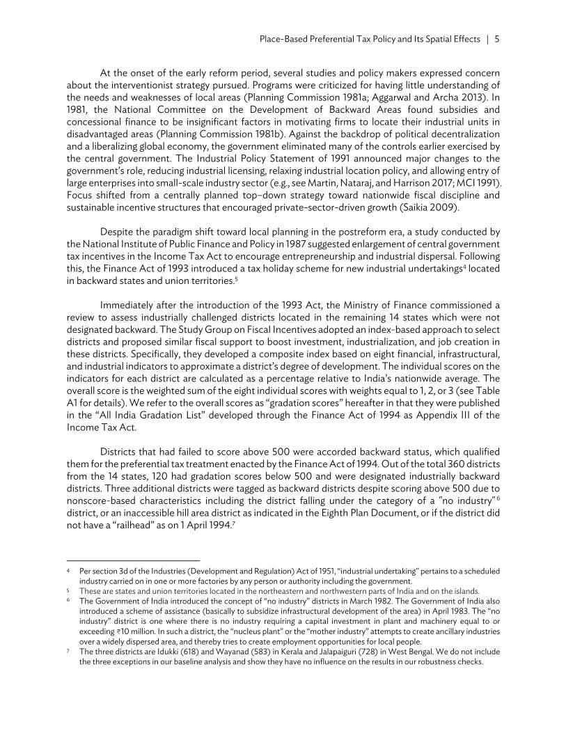
untreated districts from various neighborhoods around the cutoff score. The left panel of Table 2a compares all backward districts and nonbackward districts. The p-values of the t-tests indicate that the difference between the two sets of districts is statistically significant in several characteristics: the backward districts had smaller population, fewer main workers (who had worked 6 months or more in the survey year), fewer workers in manufacturing and trade and commerce, and fewer residential units than the nonbackward districts. The former also had substantially lower literacy rate than the latter. When we narrow the bands for comparison by focusing on the districts with scores between 251 and 850 (from Groups 2 to 5 as defined in the preceding section), as shown in the middle panel of Table 2a, the mean differences in absolute value decline in a pronounced way. Meanwhile, the differences remain negative for all variables and statistically significant for majority of them.
The right panel of Table 2a compares the backward districts from Group 3 with the
nonbackward districts from Group 4. The t-tests show none of the variables is statistically different between the two groups around the cutoff point. Importantly, the vanishing of the statistical significance is mainly driven by the diminished mean differences rather than by the enlarged standard errors of the differences due to the smaller number of districts in the comparison. In addition, the mean differences of the population, residential units, and employment variables turn positive.
8 The full list of excluded items is specified in provisions of the 11th Schedule of the Income Tax Act. Government of India,
Income Tax Department. The 11th Schedule List of Articles and Things. http://www.incometaxindia.gov.in/Acts/Income-tax%20Act,%201961/2013/102120000000027705.htm
8 | ADB Economics Working Paper Series No. 524
Table 2a: T-tests of Pretreatment District Variables in 1991
Variable
Full Sample (Groups 1 to 6) Groups 2 to 5 Groups 3 and 4 T=0
(N=237) T=1
(N=120) Diff. p-value T=0
(N=80) T=1
(N=82) Diff. p-value T=0
(N=39) T=1
(N=38) Diff p-value Population (in 1000) 2,341.7 1,901.3 –440.4 0.005 2,155.4 1,909.5 –245.9 0.14 1,882.3 2,050.5 168.1 0.517 (101.2) (94.1) (156) (111.6) (122.1) (166) (159.0) (202.7) (258.4) Main workers (in 1000) 820.7 610.1 –210.6 <.001 782.5 609.9 –172.6 0.003 641.7 678.8 37.1 0.649 (34.3) (28.5) (51.8) (43.2) (37.0) (56.7) (49.4) (64.2) (81.3) Marginal workers (in 1000) 73.1 73.5 0.4 0.954 82.7 74.9 –7.9 0.402 76.4 78.1 1.7 0.902 (3.8) (5.2) (6.5) (6.5) (6.7) (9.4) (8.2) (11.0) (13.8) Number of occupied residential 423.4 306.8 –116.6 <.001 381.2 304.5 –76.7 0.009 321.1 333.1 12.0 0.783
houses (in 1000 units) (19.6) (15.4) (29.4) (21.2) (19.7) (28.9) (26.5) (34.2) (43.4) Workers – agri fishing farming 733.0 662.9 –70.1 0.154 847.0 641.5 –205.5 0.003 680.8 707.8 27.0 0.769
(in 1000) (31.2) (31.8) (49.0) (53.8) (41.1) (67.3) (59.2) (69.7) (91.6) Workers - manufacturing 99.1 30.6 –68.6 <.001 51.4 31.6 –19.9 <.001 37.2 39.7 2.4 0.783
(in 1000) (8.8) (3.3) (12.5) (4.4) (3.6) (5.6) (5.4) (6.8) (8.7) Workers - trade and commerce 69.4 26.4 –43.0 <.001 43.3 28.0 –15.3 <.001 33.8 32.6 –1.1 0.845
(in 1000) (5.8) (1.9) (8.2) (3.0) (2.4) (3.8) (4.0) (4.2) (5.8) Area (square kilometers) 13.6 8.3 –5.2 0.344 13.8 9.9 –3.9 0.619 6.3 5.6 –0.8 0.528 (3.5) (3.6) (5.5) (6.0) (5.2) (7.9) (0.7) (0.9) (1.2) Worker participation rate (%) 38.37 37.72 –0.65 0.406 40.39 37.84 –2.54 0.024 39.36 38.12 –1.24 0.431 (0.45) (0.67) (0.78) (0.76) (0.82) (1.12) (1.09) (1.11) (1.56) Literacy rate (%) 54.95 39.38 –15.56 <.001 47.81 41.84 –5.96 0.002 47.07 45.23 –1.84 0.534 (0.94) (0.98) (1.48) (1.42) (1.22) (1.87) (2.12) (2.05) (2.94) Number of females 93.30 92.52 –0.78 0.243 94.43 92.33 –2.09 0.037 93.56 92.69 –0.87 0.534
(per 1000 males) (0.40) (0.51) (0.66) (0.73) (0.68) (0.99) (1.05) (0.91) (1.39)
Notes: From left to right, t-tests on the means of the district covariates in 1991 between the treated and untreated districts are presented with increasingly narrower samples around the cutoff point of 500. Group 1 contains districts with scores equal or below 250; Group 2 from 251 to 350; Group 3 from 351 to 500; Group 4 from 501 to 650; Group 5 from 651 to 850; Group 6 850 and above. Groups 1–3 were treated and Groups 4–6 were untreated. Standard errors are in parentheses. Source: Authors’ estimates.
Place-Based Preferential Tax Policy and Its Spatial Effects | 9
Table 2b: T-tests of District Pretreatment Variables in 1991 After Controlling for 3rd Order Polynomial of Gradation Scores
Variable
Full Sample (Groups 1 to 6) Groups 2 to 5 Groups 3 and 4T=0
(N=237) T=1
(N=120) Diff p-value T=0
(N=80) T=1
(N=82) Diff p-value T=0
(N=39) T=1
(N=38) Diff p-value Population (in 1000) 3.7 –7.1 –10.8 0.942 73.5 –26.9 –100.4 0.544 –156.8 81.1 237.9 0.361 (95.6) (93.7) (149) (110.3) (121.8) (164.9) (158.8) (203.3) (258.8) Main workers (in 1000) 15.5 –29.8 –45.3 0.36 69.6 –41.9 –111.4 0.048 –53.5 13.0 66.5 0.416 (32.4) (28.3) (49.4) (42.4) (36.8) (56.0) (49.3) (64.4) (81.4) Marginal workers (in 1000) 1.7 –3.3 –5.0 0.433 6.1 –1.9 –8.0 0.393 –0.4 1.3 1.7 0.905 (3.7) (5.2) (6.4) (6.5) (6.7) (9.4) (8.2) (11.0) (13.8) Number of occupied residential 3.6 –6.9 –10.5 0.701 24.8 –16.1 –40.9 0.154 –24.7 4.4 29.1 0.505
houses (in 1000 units) (18.1) (15.4) (27.4) (20.9) (19.6) (28.6) (26.4) (34.3) (43.4) Workers – agri fishing 35.3 –67.9 –103.2 0.033 110.1 –90.9 –201.0 0.003 –55.6 –26.1 29.4 0.749
farming (in 1000) (30.5) (31.8) (48.2) (53.8) (41.1) (67.2) (59.2) (69.7) (91.6) Workers - manufacturing –3.0 5.8 8.8 0.36 –2.6 2.1 4.7 0.381 –9.5 4.7 14.2 0.107
(in 1000) (6.7) (3.2) (9.6) (4.2) (3.4) (5.4) (5.4) (6.8) (8.7) Workers - trade and –1.0 2.0 3.0 0.644 1.7 0.9 –0.8 0.826 –3.6 2.2 5.8 0.323
commerce (in 1000) (4.6) (1.8) (6.5) (2.8) (2.3) (3.6) (4.0) (4.2) (5.8) Area (square kilometers) 1.3 –2.6 –3.9 0.476 1.4 –1.3 –2.7 0.733 –5.8 –5.9 –0.2 0.897 (3.5) (3.6) (5.5) (6.0) (5.2) (7.9) (0.7) (0.9) (1.2) Worker participation rate (%) 0.53 –1.02 –1.55 0.045 1.77 –0.88 –2.65 0.019 0.69 –0.59 –1.29 0.413 (0.43) (0.67) (0.77) (0.76) (0.82) (1.12) (1.10) (1.12) (1.56) Literacy rate (%) 0.48 –0.93 –1.42 0.284 1.70 0.62 –1.09 0.555 2.43 2.92 0.49 0.866 (0.83) (0.90) (1.32) (1.44) (1.16) (1.84) (2.13) (1.96) (2.89) Number of females 0.38 –0.74 –1.13 0.088 1.13 –0.94 –2.07 0.038 0.27 –0.59 –0.86 0.54
(per 1000 males) (0.39) (0.51) (0.66) (0.73) (0.68) (0.99) (1.05) (0.91) (1.39)
Notes: From left to right, t-tests on the mean residuals of the district covariates in 1991 after controlling for 3rd order polynomial function of the gradation scores between the treated and untreated districts are presented with increasingly narrower samples around the cutoff point of 500. Group 1 contains districts with scores equal or below 250; Group 2 from 251 to 350; Group 3 from 351 to 500; Group 4 from 501 to 650; Group 5 from 651 to 850; Group 6 850 and above. Groups 1–3 were treated and Groups 4–6 were untreated. Standard errors are in parentheses. Source: Authors’ estimates.

10 | ADB Economics Working Paper Series No. 524
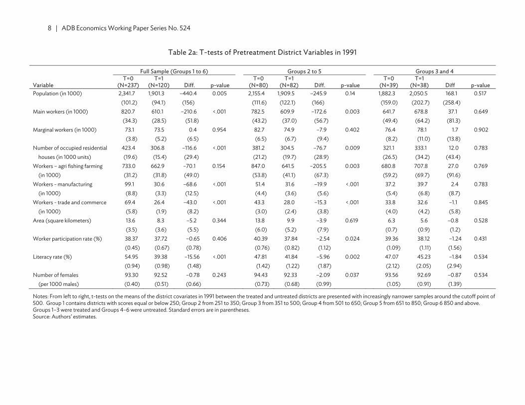
Table 2b compares the districts after controlling for a 3rd order polynomial of the gradation scores. The number of variables with statistically significant difference between all backward and all nonbackward districts was reduced from 6 to 3 when the full sample is considered, and from 8 to 4 when the districts from Groups 1 and 6 are removed. Again, no variable is statistically different when districts in Group 3 are compared to those in Group 4. The results imply that controlling for a flexible function of the gradation scores helps to balance the treated and untreated groups of districts with respect to the pretreatment characteristics when they are far from the cutoff point.
Overall, the exercise confirms that the treatment status of the backward district program is as
randomized in the neighborhood near the threshold. This neighborhood contains 38 treated districts and similar number of untreated districts.
The main regression discontinuity regressions we estimate are of the form:
1991
0 1 ( )iid d i s idd d dY T T ZS f X (1) where idY is log of number of firms or total employment in 2-digit industry i of district d in 1998. dT is a binary indicator equal to 1 if district d is designated backward, and iS is binary equal to 1 if industry i is a manufacturing industry qualified for the program. ( )df Z represents a flexible function of the gradation score and we use both first and third order polynomial functions. To get meaningful coefficient estimates for the gradation scores, we use relative scores to the cutoff point, i.e., raw scores divided by 500 as dZ . 1991
dX is an array of pretreatment district covariates measured in 1991 Census including area, population, numbers of main workers, primary workers, and manufacturing workers, all in log terms, worker participation rate, and literacy rate. i is industry fixed effect and s is state fixed effect.
In view of the intrasector differences, we further distinguish light manufacturing and heavy
manufacturing among the qualified manufacturing industries and estimate: 0
199121 ( )l h
iid d d i d d d i s idY T T T XS f ZS (2) where l
iS ( hiS ) equals 1 if industry i is one of the light (heavy) manufacturing industries (explained in
the data section).
In the above models, 1 , 2 , and are the parameters of key interest. We expect 1 and 2 to be positive had the program directly impacted the manufacturing industries in the backward districts, and to be positive had the program generated positive spillovers to other industries within the districts through input–output linkage or other agglomeration channels.
We estimate models (1) and (2) for three different samples of districts: the full sample, a sample
excluding the most challenged and most advanced districts (i.e., focusing on Groups 2 to 5), and an even narrower sample with districts from Group 3 right below and Group 4 right above the cutoff point only. When the backward districts and nonbackward districts are statistically similar to each other as in the case of the third sample, it is expected that models (1) and (2) could be estimated consistently with ordinary least squares. To the extent that controlling for function ( )df Z , pretreatment district

Place-Based Preferential Tax Policy and Its Spatial Effects | 11
covariates 1991dX and industrial and state fixed effects balances the samples consisting of more districts,
which are farther away from the cutoff, the models are also consistently estimated. To investigate program’s spatial effects, i.e., whether the program has created any (net)
displacement or agglomeration impact on the neighbor districts, we compare districts from the same group with and without any district from a treated group in their neighborhood. The idea to restrict the comparison within each group is that the districts from the same group should be similar to each other along the dimensions captured by the gradation scores. For such analysis, we could estimate the following regression models: 0
1991( )gg d d d i s ididY Z XfN (3)
where dN is equal to 1 if district d has a neighbor district from group g . g measures the spatial effects of the neighboring treated districts from group g on the own districts with negative (positive) values implying that the program’s displacement (agglomeration) effect outweighed its agglomeration (displacement) effect. We are particularly interested in the case of 3g as our estimation indicates that the program’s positive effects on firm entry and employment were largely concentrated in the districts of Group 3 (shown in the next section).
However, there may be concerns that the districts with different neighbors may differ
considerably in their geographic locations, which may partly explain their industrial development, even though they have similar gradation scores. For instance, those districts from Group 1 which have no neighboring district from Group 3 may be clustered in a remote or hilly area while those with Group 3 districts as neighbors are generally in a better “neighborhood.” To the extent that the existing controls fail to account for this geographic heterogeneity, estimation of equation (3) may yield biased g . To address this, we augment equation (3) by adding dummies of neighboring districts from other groups to enhance control for the neighborhood characteristics of district d :
196
1
10
9( )gg d d d i si idd
g
Y N Zf X
(4)
Equation (4) is estimated for the districts from each of the six groups of districts. In addition to
obtaining unbiased estimates of the spatial effects, estimating equation (4) also presents a chance of doing placebo tests. While we expect g , where 3g , to measure spatial effects of the program, if any, we expect no measurable effects by having districts from the untreated groups, i.e., Groups 4–6, in the neighborhood should our identification strategy be valid.
IV. DATA We combine establishment-level data from India’s Economic Census of 1998 and district-level data from the Primary Census Abstract of 1991 to evaluate the impact of the backward districts program.9
9 We use establishment and firm interchangeably in this study.

12 | ADB Economics Working Paper Series No. 524
The economic census, administered by the Central Statistical Organization, Ministry of Statistics and Program Implementation since 1977, provides a countrywide census of establishments engaged in all economic activities (excluding crop production and plantations). As the fourth edition, Economic Census 1998 contains key data on 30 million establishments from both rural and urban areas. For each establishment, we know the number of employees, major economic activity classified according to 1987 four-digit National Industry Classification (NIC 1987), location in terms of district and subdistrict (e.g., towns and rural blocks), type of fuel used, and so on.
We collapse the microdata to obtain the total number of firms and employment at the district
level by two-digit industry level for the analysis. Among 68 2-digit industries, which encompass 2,171 4-digit NICs, the treated industries include 7 light and 9 heavy manufacturing industries, and the untreated include 5 primary, 7 mining, 2 construction, 4 utilities, and 35 services industries. In addition, we create a category to group all the 4-digit manufacturing industries excluded from the program. However, the list of economic activities not eligible for the tax concession do not correspond to the 4-digit NIC on a one-to-one basis. More often, an excluded activity covers a subset of industries under a 4-digit NIC industry. For instance, the excluded “latex foam sponge and polyurethane foam” falls under NIC 3020 “manufacture of plastics in primary forms; manufacture of synthetic rubber,” but accounts for a small portion of the whole NIC 3020. Thus, it is largely a judgement call as to whether a 4-digit NIC involving any program-excluded activity should be put in the excluded category. We define the scope of the excluded category in three ways varying by how conservative or liberal we are in categorizing a 4-digit NIC an excluded industry. The baseline results apply a “middle path” covering 50 4-digit NICs as the excluded industries; in robustness checks we consider both more conservative (25 NICs) and more liberal approaches (91 NICs).
Economic Census 1998 uses recognized districts which had very different geographic
boundaries from those in 1991. The latter, however, was used by the program in 1994. With regard to the 14 states under consideration in our study, there are 100 more districts in Economic Census 1998 as opposed to the 360 in 1991. Fortunately, the reorganization of districts does not nullify our identification strategy since backward status accorded in 1994 was carried forward to the newly appointed districts. We construct the data with the 1991 definition of districts in order to match them with the gradation scores. For those common cases whereby an old district was split into multiple ones, we simply need to consolidate the new ones. For a few more complex cases whereby a new district was formed by parts carved out from multiple old districts, we partition the new districts using population weights developed in Kumar and Somanathan (2009), and merge the parts to their original districts.
Our final data set allows us to work with 24,840 district–industry units from 360 districts and 69
industry categories. 3,016 or 12% of the units equal zero implying there were no firms and employment in those districts by 2-digit industry cells. For the baseline results, we transform the number of firms and employment by log(Y+1) to be the dependent variables to keep all the units in the analysis. We also take log(Y) as dependent variables and leave those zero observations out of the sample in a robustness check. Although a more disaggregated unit is possible from the economic census (e.g., subdistrict by 3-digit level), the larger sample comes at the expense of obtaining extremely high frequencies of zero observations. By keeping our analysis at the district and 2-digit industry level, we try to strike a balance between sufficient nonzero observations and adequate sample size.
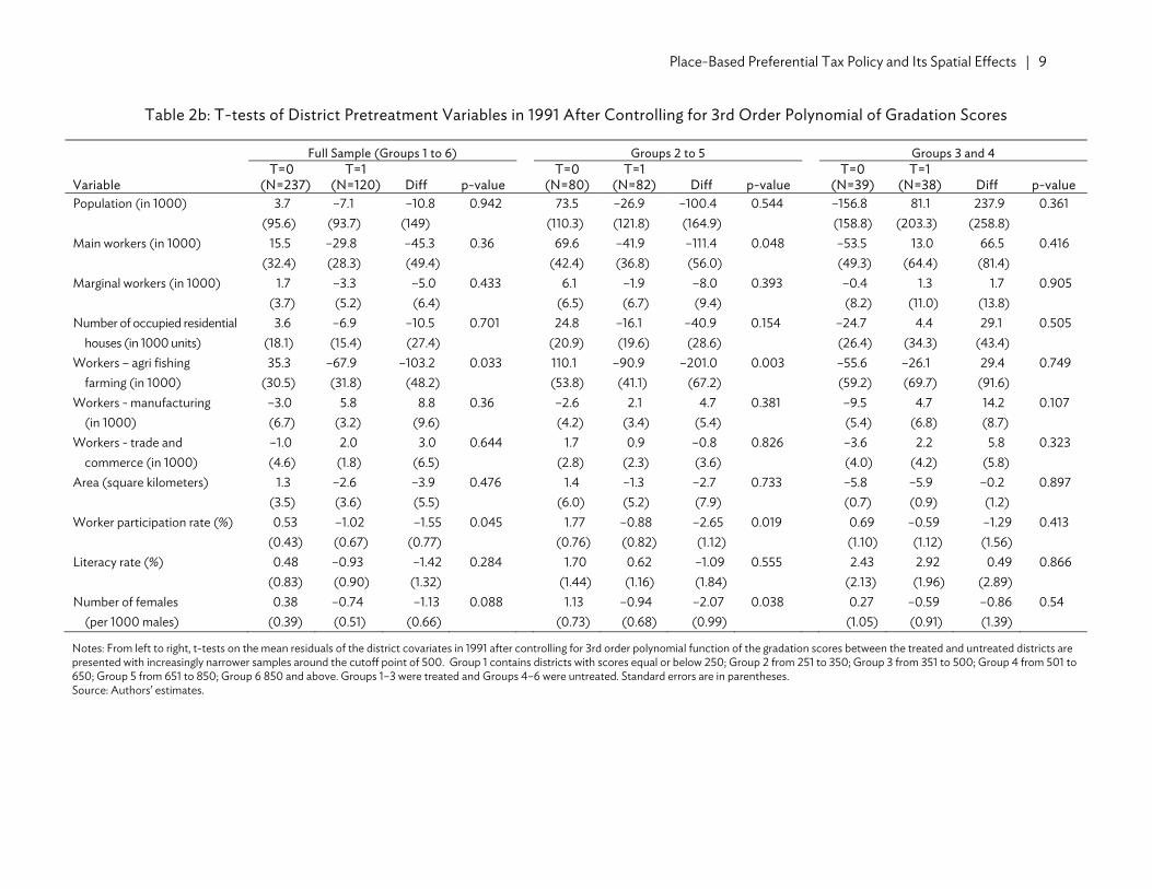
Table 3 presents summary statistics of the numbers of firms and employment by light, heavy,
and other industries for each of the six district groups. On average, there are more firms and employment in the light manufacturing industries than in the heavy manufacturing or remaining industries. As a general pattern, the average numbers of firms and employment go up with the district’s gradation score.
Place-Based Preferential Tax Policy and Its Spatial Effects | 13
However, it is interesting to note that the rising pattern shows a downward break between Group 3 and Group 4 and resumes after Group 4, whereby the mean counts of firms and employment of Group 3 are considerably larger than those of Group 4. For instance, there are on average 1,179 firms and 2,803 employees in each 2-digit industry by district unit in the light manufacturing industries of the Group 3 districts whereas the numbers drop to 963 firms and 2,528 employees in the Group 4 districts. The break is particularly evident for the light and heavy manufacturing industries, i.e., the industries eligible for the program and less so for all other industries.
Table 3: Summary Statistics of Number of Firms and Employment by District Groups and
Industrial Category
Group 1 Group 2 Group 3 Group 4 Group 5 Group 6Variables (1) (2) (3) (4) (5) (6)A. Number of Firms Light manufacturing Mean 787.6 900.7 1,179 962.7 1,109 1,295 Std 1,734 3,878 3,385 2,105 1,766 2,941 N 266 308 266 273 287 1,099Heavy manufacturing Mean 227.6 211.1 306.6 264.5 371.5 556.9 Std 505.7 519.1 712.1 478.0 641.5 1,142 N 342 396 342 351 369 1,413Other industries Mean 702.9 618.9 979.8 960.2 1,426 1,672 Std 2,792 1,800 3,732 2,992 3,835 6,099 N 2,014 2,332 2,014 2,067 2,173 8,321 B. Employment Light manufacturing Mean 1,686 2,088 2,803 2,528 3,092 5,529 Std 3,778 9,441 8,021 6,815 5,543 14,637 N 266 308 266 273 287 1,099Heavy manufacturing Mean 728.3 777.1 1,072 875.2 1,621 3,936 Std 1,923 2,101 2,865 1,719 3,118 8,805 N 342 396 342 351 369 1,413Other industries Mean 1,395 1,264 2,053 2,044 3,297 4,340 Std 6,050 3,154 6,824 5,361 8,852 14,014 N 2,014 2,332 2,014 2,067 2,173 8,321
Notes: Each block contains mean, standard deviation, and number of the 2-digit industry by district observations of each industrial category (i.e., light manufacturing, heavy manufacturing, and other) and district group. Group 1 contains districts with scores equal or below 250; Group 2 from 251 to 350; Group 3 from 351 to 500; Group 4 from 501 to 650; Group 5 from 651 to 850; Group 6 850 and above. Groups 1–3 were treated and Groups 4–6 were untreated. Source: Authors’ estimates.
The Primary Census Abstract compiled district-level data based on the Indian census data
conducted every decade. The 1991 edition of Primary Census Abstract provides us with reliable data on population, area, literacy rate, sector employment, etc., which serve as control variables in our regressions. Mean and standard deviations of these covariates by treatment status are provided in Table 2a.
V. RESULTS A. Program Impacts on the Backward Districts
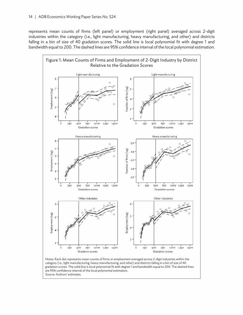
Before reporting the results, we plot the log transformed counts of firms and employment at 2-digit industry by district level against the district’s gradation scores in Figure 1. The top panel plots data on light manufacturing, the middle on heavy manufacturing, and the bottom panel on all other industries. Each dot
14 | ADB Economics Working Paper Series No. 524
represents mean counts of firms (left panel) or employment (right panel) averaged across 2-digit industries within the category (i.e., light manufacturing, heavy manufacturing, and other) and districts falling in a bin of size of 40 gradation scores. The solid line is local polynomial fit with degree 1 and bandwidth equal to 200. The dashed lines are 95% confidence interval of the local polynomial estimation.
Figure 1: Mean Counts of Firms and Employment of 2-Digit Industry by District Relative to the Gradation Scores
Notes: Each dot represents mean counts of firms or employment averaged across 2-digit industries within the category (i.e., light manufacturing, heavy manufacturing, and other) and districts falling in a bin of size of 40 gradation scores. The solid line is local polynomial fit with degree 1 and bandwidth equal to 200. The dashed lines are 95% confidence interval of the local polynomial estimation. Source: Authors’ estimates.
Place-Based Preferential Tax Policy and Its Spatial Effects | 15
In all six plots, we can see a downward gap between the two solid lines at the cutoff point where gradation score equals 500, although both lines increase in general with the scores. The gaps are larger for the light manufacturing industries than for the heavy manufacturing industries. Interestingly, visible gaps also exist for other industries which were not covered by the tax exemption program. Once we scrutinize the graphs, we can see the gaps are at least partly due to the segment of the left-hand lines near the cutoff point warping up. Finally, the graphic patterns shown on firm counts are identical to those on employment. Figure 1 implies that the program could have a positive impact on firm entry and employment in the targeted districts, especially those with relatively higher gradation scores. Moreover, industries other than qualified manufacturing in the backward districts may also have experienced growth due to the program.
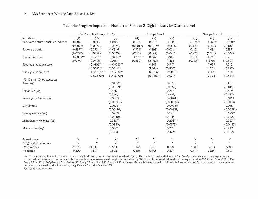
Table 4a reports estimation results of equation (1) with log transformed firm counts as
dependent variable, while Table 4b reports estimation results using employment as dependent variable. We estimated three specifications with increasing number of controls. Besides state and 2-digit industry dummies, the first specification controls for a linear term of the relative gradation score, the second controls for a third order polynomial function of the score, and the third adds district-level covariates in 1991 to the second specification. Each specification was estimated for three samples, i.e., full sample with districts from all six groups, an intermediate sample with Group 1 and Group 6 dropped (scores ranging from 251 to 850), and a sample consisting of only Group 3 and Group 4 (scores 351 to 650). The variables of primary interest are the indicator of backward district and its interaction with the indicator of qualified industries.
Column (1) of Table 4a shows that the backward districts had on average 44% fewer firms than
the nonbackward districts. The qualified manufacturing industries in the backward districts were even smaller (8%) than those in the nonbackward districts in terms of number of firms but the difference is not statistically significant. However, the estimates are more likely to suggest substantial difference in industrial development between the backward and nonbackward districts, which are not sufficiently captured by the rest of the model, than a causal effect of the program. The gradation score has a strong positive relationship with the firm counts. The coefficient estimate suggests that holding everything else constant a district of score equal to 750 (relative score equal to 1.5) has 8% more firms than a district of 250 (relative score 0.5).
When the control function ( )df Z expands from linear to third order polynomials as in column
(2), the coefficient estimate of the backward district dummy decreases in absolute value to 0.27, though still significant. Meanwhile there is little change to the coefficient of the interaction term. The three terms involving the relative gradation scores are all significant. These suggest that for all the districts whose scores span a wide range, the gradation scores in a nonlinear function can better capture the district characteristics than the linear score does. As a result, the difference between the backward and nonbackward district in firm numbers diminishes. On the other hand, Table 2b shows that the two groups of districts remain considerably different in several pretreatment measures even if we control for a flexible function of the gradation scores. Therefore, it seems appropriate to interpret the estimation that backward districts had 27% fewer firms as unexplained difference between the two groups of districts rather than program impact.
16 | ADB Economics Working Paper Series No. 524
Table 4a: Program Impacts on Number of Firms at 2-Digit Industry by District Level
Full Sample (Groups 1 to 6) Groups 2 to 5 Groups 3 and 4 Variables (1) (2) (3) (4) (5) (6) (7) (8) (9) Backward district * qualified industry –0.0848 –0.0848 –0.0866 0.161* 0.161* 0.161* 0.320** 0.320** 0.320**
(0.0877) (0.0877) (0.0875) (0.0819) (0.0819) (0.0820) (0.107) (0.107) (0.107) Backward district –0.439*** –0.273*** –0.0346 0.374* 0.393* –0.0214 0.403 0.484 0.137*
(0.0777) (0.0899) (0.0520) (0.173) (0.195) (0.0601) (0.276) (0.301) (0.0669) Gradation score 0.0835*** 0.221*** 0.0432** 1.223*** 0.342 –0.910 1.313 –10.93 –10.29
(0.0197) (0.0400) (0.0159) (0.262) (2.462) (1.468) (0.754) (16.70) (10.50) Squared gradation score –0.0106*** –0.00263** 0.549 0.547 7.699 7.210
(0.00228) (0.00112) (1.444) (0.820) (11.26) (6.892) Cubic gradation score 1.28e–08*** 3.43e–09** –0.0186 –0.00810 –0.409 –0.480
(2.59e–09) (1.42e–09) (0.0403) (0.0217) (0.794) (0.454) 1991 District Characteristics: Area (log) 0.0159** 0.0153 0.120
(0.00621) (0.0169) (0.104) Population (log) 0.586 0.267 0.849
(0.340) (0.346) (0.497) Worker participation rate 0.00333 0.00447 0.0168
(0.00807) (0.00834) (0.0133) Literacy rate 0.0123*** 0.00940** 0.0110*
(0.00174) (0.00351) (0.00591) Primary workers (log) 0.0469 0.153 0.625**
(0.0540) (0.181) (0.222) Manufacturing workers (log) 0.238*** 0.226*** 0.227***
(0.0380) (0.0375) (0.0482) Main workers (log) 0.0501 0.221 –0.947
(0.343) (0.472) (0.622)
State dummy Y Y Y Y Y Y Y Y Y 2-digit industry dummy Y Y Y Y Y Y Y Y Y Observations 24,633 24,633 24,564 11,178 11,178 11,178 5,313 5,313 5,313 R-squared 0.800 0.801 0.828 0.805 0.805 0.827 0.814 0.814 0.827
Notes: The dependent variable is number of firms 2-digit industry by district level transformed as log(Y+1). The coefficient on the Backward district * qualified industry shows the program impacts on the qualified industries in the backward districts. Gradation scores used are the original score divided by 500. Group 1 contains districts with scores equal or below 250; Group 2 from 251 to 350; Group 3 from 351 to 500; Group 4 from 501 to 650; Group 5 from 651 to 850; Group 6 850 and above. Groups 1–3 were treated and Groups 4–6 were untreated. Standard errors in parentheses are clustered at state level. *** significant at 1%, ** significant at 5%, * significant at 10%. Source: Authors’ estimates.

Place-Based Preferential Tax Policy and Its Spatial Effects | 17
Table 4b: Program Impacts on Employment at 2-Digit Industry by District Level
Full Sample (Groups 1 to 6) Groups 2 to 5 Groups 3 and 4 Variables (1) (2) (3) (4) (5) (6) (7) (8) (9) Backward district * qualified industry –0.455*** –0.455*** –0.457*** –0.00992 –0.00992 –0.00992 0.296** 0.296** 0.296**
(0.117) (0.117) (0.117) (0.0791) (0.0791) (0.0791) (0.103) (0.103) (0.103) Backward district –0.529*** –0.236** 0.0229 0.460** 0.539** 0.0963 0.441 0.473 0.149**
(0.0935) (0.0980) (0.0538) (0.195) (0.223) (0.0710) (0.310) (0.335) (0.0555) Gradation score 0.132*** 0.368*** 0.169*** 1.448*** –0.182 –1.403 1.522 –7.600 –9.514
(0.0303) (0.0489) (0.0177) (0.308) (2.513) (1.359) (0.875) (18.49) (13.13) Squared gradation score –0.0175*** –0.00884*** 1.120 1.058 5.379 6.712
(0.00283) (0.00127) (1.530) (0.744) (12.49) (8.538) Cubic gradation score 1.92e–08*** 8.73e–09*** –0.0466 –0.0345 –0.208 –0.422
(3.07e–09) (1.61e–09) (0.0445) (0.0195) (0.885) (0.568) 1991 District Characteristics: Area (log) 0.0193** 0.0144 0.166
(0.00842) (0.0209) (0.147) Population (log) 0.857** 0.604 0.721
(0.325) (0.421) (0.557) Worker participation rate 0.0102 0.0120 0.0116
(0.00830) (0.0102) (0.0140) Literacy rate 0.0136*** 0.00880*** 0.0118*
(0.00141) (0.00264) (0.00599) Primary workers (log) 0.00363 0.0249 0.405*
(0.0629) (0.155) (0.225) Manufacturing workers (log) 0.256*** 0.203*** 0.166***
(0.0437) (0.0469) (0.0259) Main workers (log) –0.0689 0.154 –0.438
(0.319) (0.505) (0.623)
State dummy Y Y Y Y Y Y Y Y Y 2-digit industry dummy Y Y Y Y Y Y Y Y Y Observations 24,633 24,633 24,564 11,178 11,178 11,178 5,313 5,313 5,313 R-squared 0.764 0.767 0.796 0.772 0.772 0.796 0.781 0.781 0.795
Notes: The dependent variable is total employment at 2-digit industry by district level transformed as log(Y+1). The coefficient on the Backward district * qualified industry shows the program impacts on the qualified industries in the backward districts. Gradation scores used are the original scores divided by 500. Group 1 contains districts with scores equal or below 250; Group 2 from 251 to 350; Group 3 from 351 to 500; Group 4 from 501 to 650; Group 5 from 651 to 850; Group 6 850 and above. Groups 1–3 were treated and Groups 4–6 were untreated. Standard errors in parentheses are clustered at state level. *** significant at 1%, ** significant at 5%, * significant at 10%. Source: Authors’ estimates.
18 | ADB Economics Working Paper Series No. 524
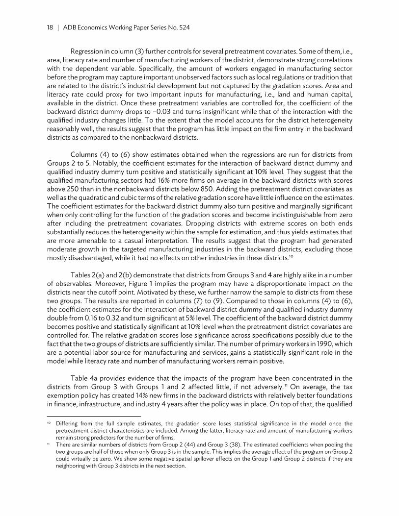
Regression in column (3) further controls for several pretreatment covariates. Some of them, i.e., area, literacy rate and number of manufacturing workers of the district, demonstrate strong correlations with the dependent variable. Specifically, the amount of workers engaged in manufacturing sector before the program may capture important unobserved factors such as local regulations or tradition that are related to the district’s industrial development but not captured by the gradation scores. Area and literacy rate could proxy for two important inputs for manufacturing, i.e., land and human capital, available in the district. Once these pretreatment variables are controlled for, the coefficient of the backward district dummy drops to –0.03 and turns insignificant while that of the interaction with the qualified industry changes little. To the extent that the model accounts for the district heterogeneity reasonably well, the results suggest that the program has little impact on the firm entry in the backward districts as compared to the nonbackward districts.
Columns (4) to (6) show estimates obtained when the regressions are run for districts from
Groups 2 to 5. Notably, the coefficient estimates for the interaction of backward district dummy and qualified industry dummy turn positive and statistically significant at 10% level. They suggest that the qualified manufacturing sectors had 16% more firms on average in the backward districts with scores above 250 than in the nonbackward districts below 850. Adding the pretreatment district covariates as well as the quadratic and cubic terms of the relative gradation score have little influence on the estimates. The coefficient estimates for the backward district dummy also turn positive and marginally significant when only controlling for the function of the gradation scores and become indistinguishable from zero after including the pretreatment covariates. Dropping districts with extreme scores on both ends substantially reduces the heterogeneity within the sample for estimation, and thus yields estimates that are more amenable to a casual interpretation. The results suggest that the program had generated moderate growth in the targeted manufacturing industries in the backward districts, excluding those mostly disadvantaged, while it had no effects on other industries in these districts.10
Tables 2(a) and 2(b) demonstrate that districts from Groups 3 and 4 are highly alike in a number
of observables. Moreover, Figure 1 implies the program may have a disproportionate impact on the districts near the cutoff point. Motivated by these, we further narrow the sample to districts from these two groups. The results are reported in columns (7) to (9). Compared to those in columns (4) to (6), the coefficient estimates for the interaction of backward district dummy and qualified industry dummy double from 0.16 to 0.32 and turn significant at 5% level. The coefficient of the backward district dummy becomes positive and statistically significant at 10% level when the pretreatment district covariates are controlled for. The relative gradation scores lose significance across specifications possibly due to the fact that the two groups of districts are sufficiently similar. The number of primary workers in 1990, which are a potential labor source for manufacturing and services, gains a statistically significant role in the model while literacy rate and number of manufacturing workers remain positive.
Table 4a provides evidence that the impacts of the program have been concentrated in the
districts from Group 3 with Groups 1 and 2 affected little, if not adversely. 11 On average, the tax exemption policy has created 14% new firms in the backward districts with relatively better foundations in finance, infrastructure, and industry 4 years after the policy was in place. On top of that, the qualified 10 Differing from the full sample estimates, the gradation score loses statistical significance in the model once the
pretreatment district characteristics are included. Among the latter, literacy rate and amount of manufacturing workers remain strong predictors for the number of firms.
11 There are similar numbers of districts from Group 2 (44) and Group 3 (38). The estimated coefficients when pooling the two groups are half of those when only Group 3 is in the sample. This implies the average effect of the program on Group 2 could virtually be zero. We show some negative spatial spillover effects on the Group 1 and Group 2 districts if they are neighboring with Group 3 districts in the next section.
Place-Based Preferential Tax Policy and Its Spatial Effects | 19
manufacturing sectors in these backward districts have experienced 32% growth in firm entry. The results are sensible in that the reduction of the tax burden may not remove the fundamental obstacles that make establishing and running enterprises unviable or unsustainable in certain areas such as lack of infrastructure, financial market, and skilled labor. On the other hand, it would only benefit those areas in which the other obstacles are less of a constraint on industrial activity should the program have any effect. It is also interesting to see that in the relatively better-off backward districts the program also led to growth in other industries such as services which were not granted tax exemption. This is probably thanks to the agglomeration effects the new manufacturing firms generated through input–output linkages.
Table 4b reports estimated models with the total employment at industry by district level as the
dependent variable. The key results, i.e., the coefficient estimates for the interaction of backward district and qualified industry dummy when the sample contains Group 3 and Group 4 districts only, are congruent to those in Table 4a. As column (9) indicates, the program increased the employment of the backward districts from Group 3 by 15% in general. In addition, the employment in the qualified manufacturing sectors went up by 30%. Both estimates are significant at 5% level. The patterns of estimates for the control variables also resemble those for the firm count models. For instance, the relative gradation scores are significant in the full sample estimation but not in the narrowest sample. Finally, the literacy rate and number of manufacturing workers stay positive and significant across samples.
It is noted that the estimates for the interaction variable differ in the employment models than
those in the firm count models estimated with full sample or intermediate sample. In the case of full sample, the qualified industries in the backwards districts had on average 46% fewer employment. Rather the program’s impact, this likely reflects the persistent gap between the backward and nonbackward districts the model is unable to fully capture. For the sample involving districts from Groups 2 to 5, the estimates suggest the program had a positive but insignificant effect in general and no effect on the qualified industries at all. This implies that the districts from Group 2 did not benefit from the program and may have been adversely affected in terms of employment growth. In sum, the evidence from examining employment echoes that on firm entry.
We further distinguish the light and heavy manufacturing sectors and see how they respond to
the program differently by estimating equation (2). The rationale is that heavy industries may respond to the tax exemption policy differently from the light ones as the former are more capital and skill intensive and thus subject to more constraints than the light ones in the underdeveloped areas. Both results for firm counts and employment are presented in Table 5.12 As expected, the interaction of the backward dummy with the light manufacturing dummy performs distinctly from that with the heavy manufacturing dummy in the models. In terms of firm entry, light manufacturing sectors in the backward districts experienced 26%–33% increases when all districts or districts from Groups 2 to 5 are considered. When we focus the sample to Groups 3 and 4, the light manufacturing grew by 55% on average on top of growth occurring to all other sectors in the backward districts. In contrast, the estimation does not suggest that the program had an economically or statistically significant impact on the heavy manufacturing industries in the backward districts.13
12 By construction, the estimates for the control variables are the same and thus left out from Table 5. 13 The significant negative estimates for the full sample are probably due to district heterogeneity not accounted for by the
models.

20 | ADB Economics Working Paper Series No. 524
Table 5: Program Impacts at 2-Digit Industry–District Level: Distinguishing Light Versus Heavy Manufacturing
Full Sample (Groups 1 to 6) Groups 2 to 5 Groups 3 and 4 Variables (1) (2) (3) (4) (5) (6) (7) (8) (9) A. Number of firms Backward district * light 0.264** 0.264** 0.263** 0.325** 0.325** 0.325** 0.551*** 0.551*** 0.551***
manufacturing (0.110) (0.110) (0.110) (0.143) (0.143) (0.143) (0.159) (0.159) (0.160) Backward district * heavy –0.356*** –0.356*** –0.358*** 0.0334 0.0334 0.0334 0.140 0.140 0.140
manufacturing (0.107) (0.107) (0.107) (0.115) (0.115) (0.115) (0.129) (0.129) (0.129) Backward district –0.439*** –0.273*** –0.0346 0.374* 0.393* –0.0214 0.403 0.484 0.137* (0.0777) (0.0899) (0.0520) (0.173) (0.195) (0.0601) (0.276) (0.301) (0.0669) R-squared 0.800 0.802 0.829 0.805 0.805 0.827 0.814 0.814 0.828 B. Employment Backward district * light 0.0288 0.0288 0.0271 0.221 0.221 0.221 0.526*** 0.526*** 0.526***
manufacturing (0.104) (0.104) (0.104) (0.124) (0.124) (0.124) (0.169) (0.169) (0.169) Backward district * heavy –0.831*** –0.831*** –0.834*** –0.190 –0.190 –0.190 0.117 0.117 0.117
manufacturing (0.164) (0.164) (0.164) (0.138) (0.138) (0.138) (0.148) (0.148) (0.148) Backward district –0.529*** –0.236** 0.0229 0.460** 0.539** 0.0963 0.441 0.473 0.149** (0.0935) (0.0980) (0.0538) (0.195) (0.223) (0.0710) (0.310) (0.335) (0.0555) R-squared 0.765 0.768 0.797 0.772 0.772 0.796 0.781 0.781 0.795 State dummy Y Y Y Y Y Y Y Y Y 2-digit industry dummy Y Y Y Y Y Y Y Y Y Linear gradation score Y N N Y N N Y N N 3rd order polynomial of gradation
scores N Y Y N Y Y N Y Y 1991 district covariates N N Y N N Y N N Y Observations 24,633 24,633 24,564 11,178 11,178 11,178 5,313 5,313 5,313
Notes: The dependent variables are number of firms and total employment at 2-digit industry by district level transformed as log(Y+1). The coefficients on the Backward district * light manufacturing and Backward district * heavy manufacturing show the program impacts on the qualified light manufacturing and heavy manufacturing, respectively, in the backward districts. Gradation scores used are the original scores divided by 500. The 1991 district covariates include log of area, population, and numbers of primary workers, manufacturing workers and main workers, worker participation rate, and literacy rate. Group 1 contains districts with scores equal or below 250; Group 2 from 251 to 350; Group 3 from 351 to 500; Group 4 from 501 to 650; Group 5 from 651 to 850; Group 6 850 and above. Groups 1–3 were treated and Groups 4–6 were untreated. Standard errors in parentheses are clustered at state level. *** significant at 1%, ** significant at 5%, * significant at 10%. Source: Authors’ estimates.
Place-Based Preferential Tax Policy and Its Spatial Effects | 21
The results on employment corroborate those on firm entry again. Compared to the districts from Group 4, districts from Group 3 had 15% more employment across all sectors and additional 53% higher employment in the light manufacturing industries by 1998. The heavy manufacturing industries did not seem to benefit from the program more than other sectors that are not covered by the program. When more districts are included for comparison, the estimated effects for the light manufacturing decrease and turn statistically insignificant, suggesting again that the program’s impacts were mainly on the better-off Group 3 districts.
Overall, Table 5 confirms our priori. It is relatively easier for the tax exemption policy to reduce
the cost disadvantages for firms producing light manufacturing goods in the challenged areas. Therefore, the program led to pronounced development in the light manufacturing sectors in the backward districts. To promote heavy manufacturing development, a more holistic approach is necessary to tackle the multiple constraints these areas face such as lack of skilled labor force, undeveloped financial markets, and poor access to national or international markets.
B. Spatial Effects of the Program We now turn to examining the program’s spatial effects. In particular, we are interested to see whether and what kind of spillover effects the treated districts have generated on their neighbors by estimating equation (4) for districts within the same gradation score group. We characterize the neighborhood of each group in Table 6 before showing the regression estimates. The top two rows show the total number of districts and their average gradation scores. Below them, each panel splits the districts from the group in the column into those with and without at least one district from the row group as well as the average gradation scores of these two subgroups. For instance, among 44 districts of Group 2, 24 districts with average gradation score equal to 298 who have one or more neighboring districts from Group 1, and the remaining 20 with average score equal to 306.5 who do not have any districts from Group 1 in their neighborhood (Panel A, column [2]).
Browsing through Table 6, a pattern of clustering can be discerned. The proportion of districts
neighbored with districts from their own group is higher than that with neighboring districts from another group. Districts from the low-score groups are more likely to have neighboring districts from the low-score groups than from the high-score groups, and likewise for the high-score districts. 14 However, clustering is far from the whole story. Within each group, there are generally 2-digit numbers of districts which have or do not have districts from any of the other groups in their neighborhood except a few cases in Panel F. Moreover, the average scores of each pair of subgroups divided by the presence of a neighboring district from another group are highly close to each other except for the subgroups of Group 6. For instance, the difference between the average scores of subgroups of Group 2 with and without a neighboring district from Group 1 is 8.5 or 2.8% of the group average (Panel A, column [2]). The picture painted here is that the geographic distribution of districts in terms of the gradation scores is fairly interlocking. Within each group, the industrial development as measured by the gradation scores did not differ systematically with their neighbor characteristics. This lends credence to our strategy to estimate the spatial effects of the program.
14 Each group has a number of neighboring districts from Group 6 because Group 6 contains more districts.
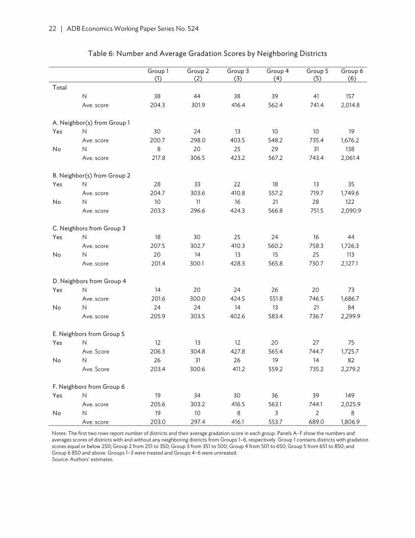
22 | ADB Economics Working Paper Series No. 524
Table 6: Number and Average Gradation Scores by Neighboring Districts
Group 1
(1) Group 2
(2) Group 3
(3) Group 4
(4) Group 5
(5) Group 6
(6) Total N 38 44 38 39 41 157 Ave. score 204.3 301.9 416.4 562.4 741.4 2,014.8 A. Neighbor(s) from Group 1 Yes N 30 24 13 10 10 19 Ave. score 200.7 298.0 403.5 548.2 735.4 1,676.2 No N 8 20 25 29 31 138 Ave. score 217.8 306.5 423.2 567.2 743.4 2,061.4 B. Neighbor(s) from Group 2 Yes N 28 33 22 18 13 35 Ave. score 204.7 303.6 410.8 557.2 719.7 1,749.6 No N 10 11 16 21 28 122 Ave. score 203.3 296.6 424.3 566.8 751.5 2,090.9 C. Neighbors from Group 3 Yes N 18 30 25 24 16 44 Ave. score 207.5 302.7 410.3 560.2 758.3 1,726.3 No N 20 14 13 15 25 113 Ave. score 201.4 300.1 428.3 565.8 730.7 2,127.1 D. Neighbors from Group 4 Yes N 14 20 24 26 20 73 Ave. score 201.6 300.0 424.5 551.8 746.5 1,686.7 No N 24 24 14 13 21 84 Ave. score 205.9 303.5 402.6 583.4 736.7 2,299.9 E. Neighbors from Group 5 Yes N 12 13 12 20 27 75 Ave. Score 206.3 304.8 427.8 565.4 744.7 1,725.7 No N 26 31 26 19 14 82 Ave. Score 203.4 300.6 411.2 559.2 735.2 2,279.2 F. Neighbors from Group 6 Yes N 19 34 30 36 39 149 Ave. score 205.6 303.2 416.5 563.1 744.1 2,025.9 No N 19 10 8 3 2 8 Ave. score 203.0 297.4 416.1 553.7 689.0 1,806.9
Notes: The first two rows report number of districts and their average gradation score in each group. Panels A–F show the numbers and averages scores of districts with and without any neighboring districts from Groups 1–6, respectively. Group 1 contains districts with gradation scores equal or below 250; Group 2 from 251 to 350; Group 3 from 351 to 500; Group 4 from 501 to 650; Group 5 from 651 to 850; and Group 6 850 and above. Groups 1–3 were treated and Groups 4–6 were untreated. Source: Authors’ estimates.

Place-Based Preferential Tax Policy and Its Spatial Effects | 23
Table 7 reports the estimation results of equation (4) for both number of firms (upper panel) and employment (lower panel). Each column presents the estimated g s for each group of districts. All models control for state dummy, 2-digit industry dummy, and third polynomial function of the gradation score and pretreatment district covariates. Take column (1) of the upper panel as an example. The results suggest that a Group 1 district with at least one neighboring district from Group 1 had 35% fewer firms than a Group 1 district without any neighboring district from Group 1, other things being equal. The difference is statistically significant at 1% level. In addition, neighboring with a district from Group 3 lowered the firm numbers by 16% with significance at 10% level. Neighbors from other groups did not have statistically significant impact on the Group 1 districts.
Conditional on other neighboring group dummies, having districts from Group 3 in the
neighborhood also had negative effects for districts of Group 2 and Group 4, with the number of firms lower by 30% in Group 2 and 23% in Group 4, relative to their peers in the same group but not neighboring with any Group 3 district. The effects are statistically significant at 5% for Group 2 and 1% level for Group 4. In contrast, a neighbor from Group 3 did not generate much difference for districts of Group 3, Group 5, or Group 6.
These spatial effects on the districts of Groups 1, 2, and 4 resulting from neighboring with Group
3 districts are attributable to the treatment of the program more than any other factor. If neighboring with Group 3 district’s proxies for some unobserved historical advantages or just spillovers from a better neighbor for Groups 1 and 2 districts, the coefficients should be positive instead of negative.15 If districts of Group 4 with a neighbor from Group 3 were at a disadvantage compared to the rest of Group 4 districts, as the negative coefficient might suggest, similar effects should be observed with respect to neighbors from Group 1 and Group 2 also.
It is intriguing to see that the above results are well supported by the regression for Group 3
districts. Column (3) shows that when districts of Group 3 had a neighbor from Group 2 or Group 4, they got better off with 20% or 30% more firms correspondingly than the other Group 3 districts who were not neighbored with any district from these two groups. Neighboring districts from Group 1 may also contribute positively to Group 3 districts’ firm counts though not significant statistically (coefficient is 0.171 with standard error 0.0967). Furthermore, having a neighbor from Groups 5 or 6 did not make a Group 3 district better or worse off.
Meanwhile, it is worth observing that similar results did not occur to the other two treated groups,
i.e., Groups 1 and 2. First, looking at the estimates in the first two rows of Table 7 indicates that no districts are positively or negatively affected by having neighboring districts from these two groups except three cases. The first two cases are that districts of Group 1 and Group 6 with any neighbor from Group 1 had fewer firms than those without. We consider that they reflect the consequence of geographic clustering instead of program effects. In other words, neighboring with Group 1 districts implies for these districts a location in more difficult areas and are thus more undeveloped industrially. The third exception is that Group 3 districts with neighbor from Group 2 had 20% more firms than other Group 3 districts. Given the earlier discussion, we believe this represents a negative spillover generated by Group 3 districts on Group 2 instead of a positive spillover from Group 2 to Group 3.
15 We do see positive but statistically insignificant coefficients for Groups 1 and 2 with neighboring districts from Group 4 and
above.
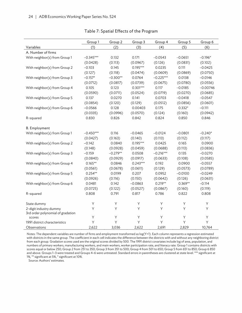
24 | ADB Economics Working Paper Series No. 524
Table 7: Spatial Effects of the Program
Group 1 Group 2 Group 3 Group 4 Group 5 Group 6 Variables (1) (2) (3) (4) (5) (6) A. Number of firms With neighbor(s) from Group 1 –0.345*** 0.132 0.171 –0.0543 –0.0651 –0.196* (0.0428) (0.113) (0.0967) (0.126) (0.0831) (0.102) With neighbor(s) from Group 2 –0.103 0.145 0.195*** 0.0235 0.111 –0.0425 (0.127) (0.118) (0.0474) (0.0609) (0.0869) (0.0750) With neighbor(s) from Group 3 –0.157* –0.300** 0.0764 –0.225*** 0.0138 –0.0146 (0.0712) (0.0817) (0.0739) (0.0675) (0.0780) (0.0556) With neighbor(s) from Group 4 0.105 0.123 0.301*** 0.117 –0.0185 –0.00746 (0.0590) (0.0711) (0.0524) (0.0719) (0.0270) (0.0685) With neighbor(s) from Group 5 0.137 0.0270 0.141 0.0703 –0.0418 –0.0547 (0.0854) (0.120) (0.129) (0.0512) (0.0856) (0.0601) With neighbor(s) from Group 6 –0.0566 0.128 0.00403 0.175 0.332* –0.111 (0.0335) (0.0996) (0.0570) (0.124) (0.160) (0.0942) R-squared 0.830 0.826 0.842 0.824 0.850 0.846 B. Employment With neighbor(s) from Group 1 –0.450*** 0.116 –0.0465 –0.0124 –0.0801 –0.240* (0.0427) (0.163) (0.140) (0.113) (0.112) (0.117) With neighbor(s) from Group 2 –0.142 0.0840 0.195*** 0.0425 0.165 0.0900 (0.148) (0.0928) (0.0459) (0.0688) (0.113) (0.0836) With neighbor(s) from Group 3 –0.159 –0.279** 0.0508 –0.216*** 0.135 –0.0270 (0.0840) (0.0929) (0.0917) (0.0633) (0.108) (0.0585) With neighbor(s) from Group 4 0.165** 0.0846 0.243*** 0.192 0.0900 –0.0557 (0.0561) (0.0678) (0.0611) (0.129) (0.0573) (0.0789) With neighbor(s) from Group 5 0.254** 0.0199 0.207 0.0952 –0.0100 –0.0249 (0.0926) (0.116) (0.150) (0.0642) (0.126) (0.0631) With neighbor(s) from Group 6 0.0481 0.142 –0.0863 0.219** 0.369** –0.114 (0.0725) (0.122) (0.0527) (0.0867) (0.160) (0.119) R-squared 0.808 0.791 0.817 0.786 0.822 0.808 State dummy Y Y Y Y Y Y 2-digit industry dummy Y Y Y Y Y Y 3rd order polynomial of gradation
scores Y Y Y Y Y Y 1991 district characteristics Y Y Y Y Y Y Observations 2,622 3,036 2,622 2,691 2,829 10,764
Notes: The dependent variables are number of firms and employment transformed as log(Y+1). Each column represents a regression estimated with districts in the same group. The coefficient in each cell indicates the difference between the districts with and without any neighboring district from each group. Gradation scores used are the original scores divided by 500. The 1991 district covariates include log of area, population, and numbers of primary workers, manufacturing workers, and main workers, worker participation rate, and literacy rate. Group 1 contains districts with scores equal or below 250; Group 2 from 251 to 350; Group 3 from 351 to 500; Group 4 from 501 to 650; Group 5 from 651 to 850; Group 6 850 and above. Groups 1–3 were treated and Groups 4–6 were untreated. Standard errors in parentheses are clustered at state level. *** significant at 1%, ** significant at 5%, * significant at 10%.
Source: Authors’ estimates.

Place-Based Preferential Tax Policy and Its Spatial Effects | 25
Second, when we examine the regressions for Group 1 and Group 2, it is clear that these districts were not affected by their neighbors except those from Group 3. Had they generated any spatial spillovers, we expect to observe a symmetric reflection in these regressions as we see in the column (3) for Group 3. To sum, although districts of Group 1 and Group 2 were treated by the program, we do not find any significant spatial effects from them to the neighboring districts. This is indeed consistent with our finding in the preceding section that the program impacts mainly fell on the districts of Group 3.
Results for employment again demonstrate high consistency with those for firm counts. Districts
of Group 2 that had neighboring districts from Group 3 had on average 28% fewer employment than the rest of the districts in the same group, while Group 4 districts in the same context had 22% fewer employment. Correspondingly, the employment size of districts of Group 3 was 20% larger with one or more Group 2 districts or 24% larger with Group 4 in their neighborhood. Unlike in the firm number models, the spatial effects from Group 3 on Group 1 districts are inconclusive though.
It is noted that the districts of Group 1 with neighboring districts from Group 4 or Group 5 had
higher employment than those without. The differences are likely because the former is located in regions more conducive to economic activity than the latter instead of being due to spatial spillovers caused by the program since the districts of Groups 4 and 5 did not seem to be adversely affected by having a neighbor from Group 1. Neighboring with Group 6 districts also predicts higher employment for districts of Groups 4 and 5. The program should not play a role here since none of the three groups was treated.
We conclude that the relatively better-performing backward districts, whom the program mainly
benefited, had shown negative spillovers to the districts spatially as well as economically close to them. Though the spillovers may vary by industry and could be positive to certain areas or industries due to potential agglomeration effects, overall they are negative and essentially displace firms in both untreated and treated districts which were relatively weaker for economic development. For those that were substantially stronger than the best treated districts, such as those in Groups 5 and 6, the program did not have any adverse effect on them. Finally, the more challenged districts, which accounted for a majority among all the backward districts, did not only fail to benefit from the program, but also lost industrial development opportunity to their neighbors who were relatively stronger and covered by the program as well.
Regressions in Table 7 offer a chance for us to undertake placebo tests to validate the above
conclusion further. The idea is that if the spatial effects identified with respect to the districts of Group 3 were attributable to some unobserved confounding factors, say geographic or historical (dis)advantages imperfectly controlled for in the model rather than to the program treatment, it is likely that we would observe similar spatial spillovers from districts of Groups 4, 5, or 6 even though they were not treated by the program.
The results dismiss such alternative story about the spatial effects. Generally, neighboring with
districts from Groups 4, 5, or 6 did not lead to any statistically significant effects, especially negative effects, on districts with gradation scores below them. 16 In addition, neighboring with Group 4 (5) districts did not make Group 5 (6) districts worse off. Finally, the districts from Groups 4, 5, or 6 did not benefit from neighboring with districts one group above or one group below them like Group 3 districts
16 The few significant estimates, particularly those involving employment for Group 1 districts have been noted and discussed
earlier.
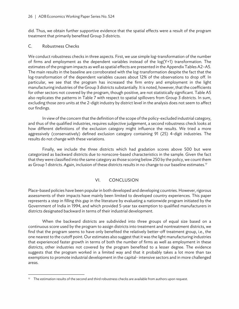
26 | ADB Economics Working Paper Series No. 524
did. Thus, we obtain further supportive evidence that the spatial effects were a result of the program treatment that primarily benefited Group 3 districts.
C. Robustness Checks
We conduct robustness checks in three aspects. First, we use simple log-transformation of the number of firms and employment as the dependent variables instead of the log(Y+1) transformation. The estimates of the program impacts as well as spatial effects are presented in the Appendix Tables A2–A5. The main results in the baseline are corroborated with the log-transformation despite the fact that the log-transformation of the dependent variables causes about 12% of the observations to drop off. In particular, we see that the program has increased the firm entry and employment in the light manufacturing industries of the Group 3 districts substantially. It is noted, however, that the coefficients for other sectors not covered by the program, though positive, are not statistically significant. Table A5 also replicates the patterns in Table 7 with respect to spatial spillovers from Group 3 districts. In sum, excluding those zero units at the 2-digit industry by district level in the analysis does not seem to affect our findings.
In view of the concern that the definition of the scope of the policy-excluded industrial category,
and thus of the qualified industries, requires subjective judgement, a second robustness check looks at how different definitions of the exclusion category might influence the results. We tried a more aggressively (conservatively) defined exclusion category containing 91 (25) 4-digit industries. The results do not change with these variations.
Finally, we include the three districts which had gradation scores above 500 but were
categorized as backward districts due to nonscore-based characteristics in the sample. Given the fact that they were classified into the same category as those scoring below 250 by the policy, we count them as Group 1 districts. Again, inclusion of these districts results in no change to our baseline estimates.17
VI. CONCLUSION Place-based policies have been popular in both developed and developing countries. However, rigorous assessments of their impacts have mainly been limited to developed country experiences. This paper represents a step in filling this gap in the literature by evaluating a nationwide program initiated by the Government of India in 1994, and which provided 5-year tax exemption to qualified manufacturers in districts designated backward in terms of their industrial development.
When the backward districts are subdivided into three groups of equal size based on a
continuous score used by the program to assign districts into treatment and nontreatment districts, we find that the program seems to have only benefited the relatively better-off treatment group, i.e., the one nearest to the cutoff point. Our estimates also suggest that it was the light manufacturing industries that experienced faster growth in terms of both the number of firms as well as employment in these districts; other industries not covered by the program benefited to a lesser degree. The evidence suggests that the program worked in a limited way and that it probably takes a lot more than tax exemptions to promote industrial development in the capital- intensive sectors and in more challenged areas.
17 The estimation results of the second and third robustness checks are available from authors upon request.
Place-Based Preferential Tax Policy and Its Spatial Effects | 27
Further examining the possible spatial spillovers of the program, we find evidence consistent with the idea that the program generated considerable displacement between the better-off treated districts and their neighbors, which were either treated but weaker in terms of their economic environment or not treated and having only a slightly better economic environment than the treated districts. This further casts doubts on the program’s effectiveness from a national perspective.
It is interesting to note that if the gap between the treated districts and their neighbors were
significantly large, the negative spillovers would unlikely take place across space. For example, the more challenged districts from Group 1 and Group 2 did not demonstrate any spatial effects on other groups in their neighborhood. Similarly, districts of Group 3 did not adversely affect neighboring districts of Group 5 and Group 6. This may explain in part why Chaurey (2016) does not find any spatial spillovers when he assessed India’s New Industrial Policy. Himachal Pradesh, one of the two states covered by the policy, was designated a backward state in 1993 and its neighboring state Punjab had all districts from Group 6.18
Other than policies that offer tax exemptions to promote industrial development in targeted
areas, special economic zones or industrial parks have attracted attention of policy makers in developing countries. Compared to preferential tax programs, the latter may better address local disadvantages or help reveal the comparative advantages of different areas. It would be interesting to compare these different place-based policies quantitatively. However, spatial spillovers remain a concern for such polices from the perspective of overall development or welfare. Finally, India seems to have a relatively low internal migration rate (Munshi and Rosenzweig 2009). Industrialization may well progress faster with policies that facilitate the movement of labor to places where manufacturing has a comparative advantage (such as through more affordable housing) than policies that try and take manufacturing to disadvantaged locations. Future research aimed at this issue would be a useful complement to the work presented in this paper.
18 Differences in the two policies may also explain the divergent findings regarding spatial effects across the two studies. The
New Industrial Policy provided tax exemption and capital subsidies to both new and existing firms while the Backward District Policy only provided tax exemption to the new firms. This is a topic to be further investigated.

APPENDIXES
Table A1: Indicators Used to Construct Gradation Scores to Identify Backward Districts
Criteria Weights IndicatorsFinancial 3 Per capital credit given by scheduled commercial banks 2 Per capital deposit received by scheduled commercial banks Infrastructural 1 Phones per thousand population 2 Per capita power consumption 1 Urbanization (urban population of a district as a proportion of total population) 1 Metaled roads per 100 square kilometersIndustrial 3 Workers in registered factories per thousand population (excluding electrical
undertakings and bidi & cigar units) 2 Per capital gross value added from registered manufacturing sector
Source: Government of India, Ministry of Finance, Department of Revenue (Central Board of Direct Taxes). “All India Gradation List.” Appendix III of the Income Tax Act (S.O. 635 [E]). Notification on 3 September 1997. New Delhi. http://ncrpb.nic.in/pdf_files/16_AnnexureVII_part1_cma.pdf

30 | Appendixes
Table A2: Program Impacts on Firm Count At 2-Digit Industry–District Level (Dependent Variable Log-Transformed)
Full Sample (Groups 1 to 6) Groups 2 to 5 Groups 3 and 4 Variables (1) (2) (3) (4) (5) (6) (7) (8) (9) Backward district * qualified industry –0.000252 –0.00138 –0.00473 0.218** 0.218* 0.218** 0.313** 0.313** 0.314** (0.0880) (0.0878) (0.0845) (0.100) (0.100) (0.0982) (0.108) (0.108) (0.111) Backward district –0.458*** –0.297** –0.0559 0.338 0.362 –0.0694 0.394 0.464 0.0953 (0.0857) (0.1000) (0.0567) (0.206) (0.226) (0.0818) (0.311) (0.346) (0.0709) Gradation score 0.0858*** 0.217*** 0.0322* 1.211*** 0.0204 –1.481 1.298 –9.461 –8.503 (0.0194) (0.0423) (0.0165) (0.304) (2.543) (1.608) (0.819) (17.54) (8.809) Squared gradation score –0.0101*** –0.00185* 0.735 0.837 6.744 6.016 (0.00240) (0.000957) (1.479) (0.895) (11.78) (5.777) Cubic gradation score 1.22e–08*** 2.38e–09* –0.0244 –0.0163 –0.353 –0.409 (2.79e–09) (1.23e–09) (0.0408) (0.0242) (0.813) (0.377) 1991 District Characteristics: Area (log) 0.0228*** 0.0226 0.120 (0.00632) (0.0174) (0.0899) Population (log) 0.441 0.189 0.661 (0.364) (0.393) (0.444) Worker participation rate –0.00231 0.000157 0.0121 (0.00856) (0.00897) (0.0126) Literacy rate 0.0122*** 0.00979** 0.0110* (0.00210) (0.00384) (0.00564) Primary workers (log) 0.0365 0.149 0.618** (0.0454) (0.197) (0.199) Manufacturing workers (log) 0.253*** 0.266*** 0.270*** (0.0357) (0.0392) (0.0542) Main workers (log) 0.218 0.313 –0.751 (0.370) (0.524) (0.546) State dummy Y Y Y Y Y Y Y Y Y 2-digit industry dummy Y Y Y Y Y Y Y Y Y Observations 21,643 21,643 21,581 9,689 9,689 9,689 4,619 4,619 4,619 R-squared 0.748 0.750 0.786 0.753 0.753 0.784 0.764 0.764 0.783
Notes: The dependent variable is number of firms’ 2-digit industry by district level transformed as log(Y). The coefficient on the Backward district * qualified industry shows the program impacts on the qualified industries in the backward districts. Gradation scores used are the original scores divided by 500. Group 1 contains districts with scores equal or below 250; Group 2 from 251 to 350; Group 3 from 351 to 500; Group 4 from 501 to 650; Group 5 from 651 to 850; Group 6 850 and above. Groups 1–3 were treated and Groups 4–6 were untreated. Standard errors in parentheses are clustered at state level. *** significant at 1%, ** significant at 5%, * significant at 10%. Source: Authors’ estimates.
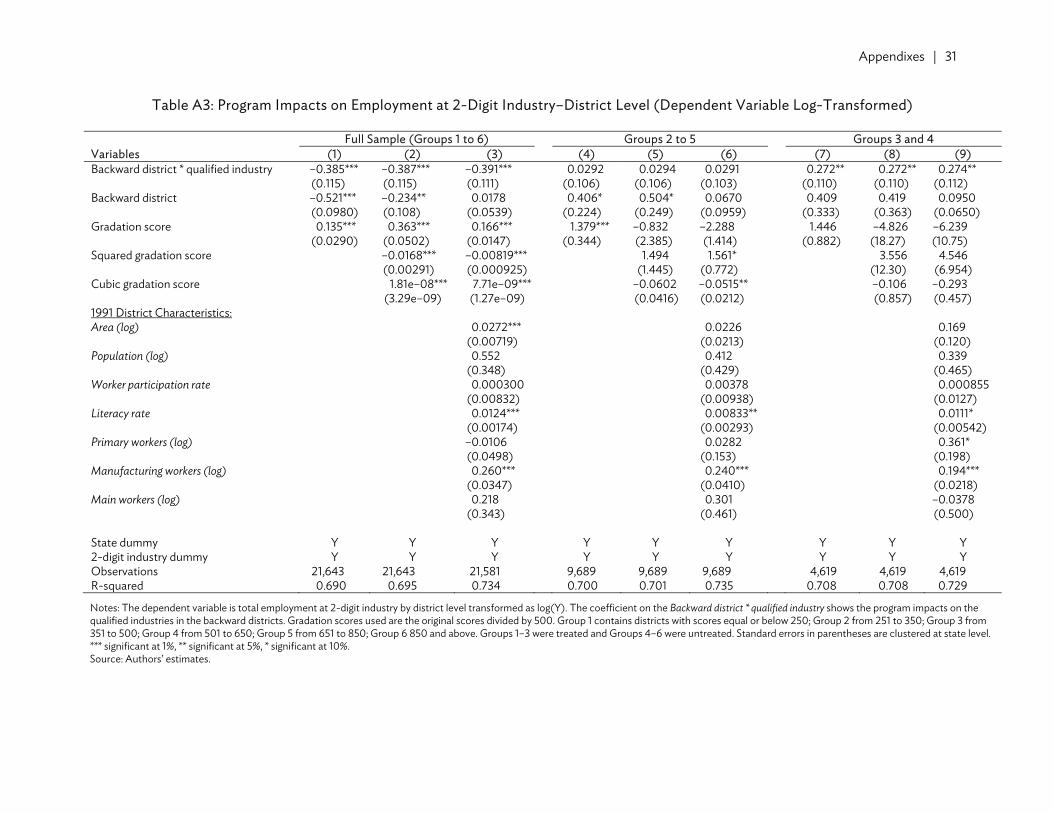
Appendixes | 31
Table A3: Program Impacts on Employment at 2-Digit Industry–District Level (Dependent Variable Log-Transformed)
Full Sample (Groups 1 to 6) Groups 2 to 5 Groups 3 and 4Variables (1) (2) (3) (4) (5) (6) (7) (8) (9)Backward district * qualified industry –0.385*** –0.387*** –0.391*** 0.0292 0.0294 0.0291 0.272** 0.272** 0.274** (0.115) (0.115) (0.111) (0.106) (0.106) (0.103) (0.110) (0.110) (0.112)Backward district –0.521*** –0.234** 0.0178 0.406* 0.504* 0.0670 0.409 0.419 0.0950 (0.0980) (0.108) (0.0539) (0.224) (0.249) (0.0959) (0.333) (0.363) (0.0650)Gradation score 0.135*** 0.363*** 0.166*** 1.379*** –0.832 –2.288 1.446 –4.826 –6.239 (0.0290) (0.0502) (0.0147) (0.344) (2.385) (1.414) (0.882) (18.27) (10.75)Squared gradation score –0.0168*** –0.00819*** 1.494 1.561* 3.556 4.546 (0.00291) (0.000925) (1.445) (0.772) (12.30) (6.954)Cubic gradation score 1.81e–08*** 7.71e–09*** –0.0602 –0.0515** –0.106 –0.293 (3.29e–09) (1.27e–09) (0.0416) (0.0212) (0.857) (0.457)1991 District Characteristics: Area (log) 0.0272*** 0.0226 0.169 (0.00719) (0.0213) (0.120)Population (log) 0.552 0.412 0.339 (0.348) (0.429) (0.465)Worker participation rate 0.000300 0.00378 0.000855 (0.00832) (0.00938) (0.0127)Literacy rate 0.0124*** 0.00833** 0.0111* (0.00174) (0.00293) (0.00542) Primary workers (log) –0.0106 0.0282 0.361* (0.0498) (0.153) (0.198)Manufacturing workers (log) 0.260*** 0.240*** 0.194*** (0.0347) (0.0410) (0.0218)Main workers (log) 0.218 0.301 –0.0378 (0.343) (0.461) (0.500) State dummy Y Y Y Y Y Y Y Y Y2-digit industry dummy Y Y Y Y Y Y Y Y YObservations 21,643 21,643 21,581 9,689 9,689 9,689 4,619 4,619 4,619R-squared 0.690 0.695 0.734 0.700 0.701 0.735 0.708 0.708 0.729
Notes: The dependent variable is total employment at 2-digit industry by district level transformed as log(Y). The coefficient on the Backward district * qualified industry shows the program impacts on the qualified industries in the backward districts. Gradation scores used are the original scores divided by 500. Group 1 contains districts with scores equal or below 250; Group 2 from 251 to 350; Group 3 from 351 to 500; Group 4 from 501 to 650; Group 5 from 651 to 850; Group 6 850 and above. Groups 1–3 were treated and Groups 4–6 were untreated. Standard errors in parentheses are clustered at state level. *** significant at 1%, ** significant at 5%, * significant at 10%. Source: Authors’ estimates.
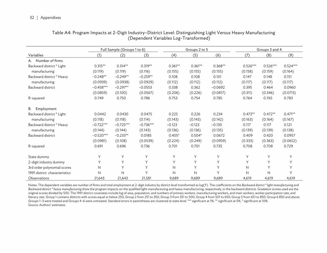
32 | Appendixes
Table A4: Program Impacts at 2-Digit Industry–District Level: Distinguishing Light Versus Heavy Manufacturing (Dependent Variables Log-Transformed)
Full Sample (Groups 1 to 6) Groups 2 to 5 Groups 3 and 4 Variables (1) (2) (3) (4) (5) (6) (7) (8) (9) A. Number of firms Backward district * Light 0.315** 0.314** 0.319** 0.361** 0.361** 0.368** 0.526*** 0.526*** 0.524***
manufacturing (0.119) (0.119) (0.116) (0.155) (0.155) (0.155) (0.158) (0.159) (0.164) Backward district * Heavy –0.248** –0.249** –0.259** 0.108 0.108 0.101 0.147 0.148 0.151
manufacturing (0.0939) (0.0938) (0.0929) (0.112) (0.112) (0.112) (0.117) (0.117) (0.117) Backward district –0.458*** –0.297** –0.0553 0.338 0.362 –0.0692 0.395 0.464 0.0960 (0.0859) (0.100) (0.0567) (0.206) (0.226) (0.0817) (0.311) (0.346) (0.0713) R-squared 0.749 0.750 0.786 0.753 0.754 0.785 0.764 0.765 0.783 B. Employment Backward district * Light 0.0442 0.0430 0.0475 0.225 0.226 0.234 0.473** 0.472** 0.471**
manufacturing (0.118) (0.118) (0.114) (0.143) (0.143) (0.142) (0.163) (0.164) (0.167) Backward district * Heavy –0.722*** –0.725*** –0.736*** –0.123 –0.123 –0.130 0.117 0.117 0.121
manufacturing (0.144) (0.144) (0.143) (0.136) (0.136) (0.135) (0.139) (0.139) (0.138) Backward district –0.520*** –0.233** 0.0185 0.405* 0.504* 0.0672 0.409 0.420 0.0957 (0.0981) (0.108) (0.0539) (0.224) (0.249) (0.0959) (0.333) (0.363) (0.0652) R-squared 0.691 0.696 0.736 0.701 0.701 0.735 0.708 0.708 0.729 State dummy Y Y Y Y Y Y Y Y Y 2-digit industry dummy Y Y Y Y Y Y Y Y Y 3rd order polynomial scores N Y Y N Y Y N Y Y 1991 district characteristics N N Y N N Y N N Y Observations 21,643 21,643 21,581 9,689 9,689 9,689 4,619 4,619 4,619
Notes: The dependent variables are number of firms and total employment at 2-digit industry by district level transformed as log(Y). The coefficients on the Backward district * light manufacturing and Backward district * heavy manufacturing show the program impacts on the qualified light manufacturing and heavy manufacturing, respectively, in the backward districts. Gradation scores used are the original scores divided by 500. The 1991 district covariates include log of area, population, and numbers of primary workers, manufacturing workers, and main workers, worker participation rate, and literacy rate. Group 1 contains districts with scores equal or below 250; Group 2 from 251 to 350; Group 3 from 351 to 500; Group 4 from 501 to 650; Group 5 from 651 to 850; Group 6 850 and above. Groups 1–3 were treated and Groups 4–6 were untreated. Standard errors in parentheses are clustered at state level. *** significant at 1%, ** significant at 5%, * significant at 10%. Source: Authors’ estimates.
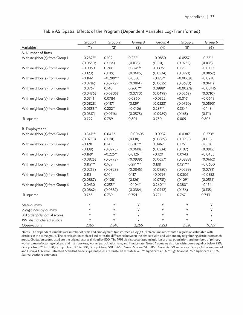
Appendixes | 33
Table A5: Spatial Effects of the Program (Dependent Variables Log-Transformed)
Group 1 Group 2 Group 3 Group 4 Group 5 Group 6 Variables (1) (2) (3) (4) (5) (6) A. Number of firms With neighbor(s) from Group 1 –0.282*** 0.102 0.222* –0.0850 –0.0557 –0.221* (0.0550) (0.134) (0.108) (0.110) (0.0735) (0.106) With neighbor(s) from Group 2 –0.0950 0.206 0.224*** 0.0396 0.125 –0.0722 (0.123) (0.119) (0.0605) (0.0534) (0.0921) (0.0852) With neighbor(s) from Group 3 –0.166* –0.288*** 0.0550 –0.173** –0.00628 –0.0278 (0.0716) (0.0772) (0.0814) (0.0635) (0.0680) (0.0611) With neighbor(s) from Group 4 0.0767 0.140 0.360*** 0.0998* –0.00376 –0.00415 (0.0436) (0.0805) (0.0770) (0.0498) (0.0263) (0.0710) With neighbor(s) from Group 5 0.0341 0.0784 0.0960 –0.0322 –0.0161 –0.0648 (0.0828) (0.117) (0.129) (0.0523) (0.0720) (0.0590) With neighbor(s) from Group 6 –0.0855** 0.222** –0.0106 0.237** 0.334* –0.148 (0.0317) (0.0716) (0.0578) (0.0989) (0.165) (0.111) R-squared 0.799 0.789 0.801 0.780 0.809 0.805
B. Employment With neighbor(s) from Group 1 –0.347*** 0.0422 –0.00605 –0.0952 –0.0387 –0.273** (0.0758) (0.181) (0.138) (0.0869) (0.0955) (0.115) With neighbor(s) from Group 2 –0.120 0.141 0.230*** 0.0467 0.179 0.0530 (0.138) (0.0975) (0.0608) (0.0534) (0.107) (0.0915) With neighbor(s) from Group 3 –0.169* –0.226** 0.0126 –0.120 0.0943 –0.0485 (0.0825) (0.0793) (0.0939) (0.0657) (0.0888) (0.0662) With neighbor(s) from Group 4 0.115*** 0.109 0.291*** 0.138 0.121*** –0.0600 (0.0255) (0.0828) (0.0845) (0.0950) (0.0299) (0.0731) With neighbor(s) from Group 5 0.113 0.104 0.117 –0.0795 0.0306 –0.0352 (0.0887) (0.108) (0.126) (0.0731) (0.109) (0.0531) With neighbor(s) from Group 6 0.0430 0.255** –0.104** 0.260*** 0.380** –0.154 (0.0862) (0.0887) (0.0384) (0.0542) (0.156) (0.135) R-squared 0.768 0.739 0.754 0.721 0.767 0.743
State dummy Y Y Y Y Y Y 2-digit industry dummy Y Y Y Y Y Y 3rd order polynomial scores Y Y Y Y Y Y 1991 district characteristics Y Y Y Y Y Y Observations 2,165 2,540 2,266 2,353 2,530 9,727
Notes: The dependent variables are number of firms and employment transformed as log(Y). Each column represents a regression estimated with districts in the same group. The coefficient in each cell indicates the difference between the districts with and without any neighboring district from each group. Gradation scores used are the original scores divided by 500. The 1991 district covariates include log of area, population, and numbers of primary workers, manufacturing workers, and main workers, worker participation rate, and literacy rate. Group 1 contains districts with scores equal or below 250; Group 2 from 251 to 350; Group 3 from 351 to 500; Group 4 from 501 to 650; Group 5 from 651 to 850; Group 6 850 and above. Groups 1–3 were treated and Groups 4–6 were untreated. Standard errors in parentheses are clustered at state level. *** significant at 1%, ** significant at 5%, * significant at 10%. Source: Authors’ estimates.

REFERENCES Aggarwal, Aradhna, and Prakash Singh Archa. 2013. “Regional Development Policies in India.” In The
Internal Geography of Trade: Lagging Regions and Global Markets, edited by Thomas Farole, 229–55. Washington, DC: The World Bank.
Bartik, Timothy J. 1991. Who Benefits from State and Local Economic Development Policies? Kalamazoo,
MR: W.E. Upjohn Institute for Employment Research. Busso, Matias, Jesse Gregory, and Patrick Kline. 2013. “Assessing the Incidence and Efficiency of a
Prominent Place-Based Policy.” American Economic Review 103 (2): 897–947. Chaurey, Ritam. 2016. “Location-Based Tax Incentives: Evidence from India.” Journal of Public Economics.
doi:10.1016/j.jpubeco.2016.08.013 Duranton, Gilles, Laurent Gobillon, and Henry G. Overman. 2011. “Assessing the Effects of Local
Taxation Using Micro Geographic Data.” The Economic Journal 121 (555): 1017–46. Freedman, Matthew. 2013. “Targeted Business Incentives and Local Labor Markets.” Journal of Human
Resources 48 (2): 311–44. Ghosh, Buddhadeb, Sugata Marjit, and Chiranjib Neogi. 1998. “Economic Growth and Regional
Divergence in India, 1960 to 1995.” Economic and Political Weekly 33 (26): 1623–30. Givord, Pauline, Roland Rathelot, and Patrick Sillard. 2013. “Place-Based Tax Exemptions and
Displacement Effects: An Evaluation of the Zones Franches Urbaines Program.” Regional Science and Urban Economics 43 (1): 151–63.
Government of India, Income Tax Department. “The 11th Schedule List of Articles or Things.”
http://www.incometaxindia.gov.in/Acts/Income-tax%20Act,%201961/2013/1021200000000 27705.htm
Government of India, Ministry of Commerce and Industry (MCI). 1977. “Statement of Industrial Policy.”
New Delhi. ————. 1991. “Statement of Industrial Policy.” New Delhi. Government of India, Ministry of Finance, Department of Revenue (Central Board of Direct Taxes).
“All India Gradation List.” Appendix III of the Income Tax Act (S.O. 635 [E]). Notification on 3 September 1997. New Delhi. http://ncrpb.nic.in/pdf_files/16_AnnexureVII_part1_cma.pdf
Government of India, Planning Commission. 1961. “Third Five Year Plan (1961–1966).” New Delhi. ————. 1966. “Fourth Five Year Plan (1966–1971).” New Delhi. ————. 1981a. “Report on General Issues Relating to Backward Areas Development.”
http://planningcommission.nic.in/reports/publications/pb80_NCDBAgn.pdf
36 | References
————. 1981b. Report on Industrial Dispersal the National Committee on Development of Background Areas. http://planningcommission.nic.in/reports/publications/ pub_inddis.pdf
Guimaraes, Paulo, Octávio Figueiredo, and Douglas Woodward. 2004. “Industrial Location Modeling:
Extending the Random Utility Framework.” Journal of Regional Science 44 (1): 1–20. Hanson, Andrew. 2009. “Local Employment, Poverty, and Property Value Effects of Geographically
Targeted Tax Incentives: An Instrumental Variables Approach.” Regional Science and Urban Economics 39 (6): 721–31.
Kumar, Hemanshu, and Rohini Somanathan. 2009. “Mapping Indian Districts Across Census Years,
1971–2001.” Centre for Development Economics Working Paper No. 176 Lee, David S., and Thomas Lemieuxa. 2010. “Regression Discontinuity Designs in Economics.” Journal of
Economic Literature 48 (2): 281–355. Martin, Leslie A., Shanthi Nataraj, and Ann E. Harrison. 2017. “In With the Big, Out With the Small:
Removing Small-Scale Reservations in India.” American Economic Review 107 (2): 354–86. Munshi, Kaivan, and Mark Rosenzweig. 2009. “Why is Mobility in India so Low? Social Insurance,
Inequality, and Growth.” NBER Working Paper No. 14850. Neumark, David, and Jed Kolko. 2010. “Do Enterprise Zones Create Jobs? Evidence from California’s
Enterprise Zone Program.” Journal of Urban Economics 68 (1): 1–19. Neumark, David, and Helen Simpson. 2015. “Place-Based Policies.” In Handbook of Regional and Urban
Economics Vol. 5, edited by Gilles Duranton, J. Vernon Henderson, and William C. Strange, 1197–287. North Holland: Elsevier.
Rathelot, Roland, and Patrick Sillard. 2008. “The Importance of Local Corporate Taxes in Business
Location Decisions: Evidence from French Micro Data.” The Economic Journal 118 (527): 499–514.
Saikia. Dilip. 2009. “Industrial Location in India Under Liberalisation.” Munich Personal Research Papers
in Economics Archive Paper. No. 27821. Singhi, M. C. 2012. “Report on the Role of Incentives in the Development of Industrially Backward
States/UTs.” Office of the Economic Adviser, Paper No. 39. http://www.eaindustry.nic.in/ discussion_papers/Development_of_backward_areas.pdf
Wang, Jin. 2013. “The Economic Impact of Special Economic Zones: Evidence from Chinese
Municipalities.” Journal of Development Economics 101 (C): 133–47.

ASIAN DEVELOPMENT BANK
AsiAn Development BAnk6 ADB Avenue, Mandaluyong City1550 Metro Manila, Philippineswww.adb.org
Place-Based Preferential Tax Policy and Its Spatial Effects: Evidence from India’s Program on Industrially Backward Districts
Place-based policies aimed at enhancing economic performance of certain areas within a country or region have been popular in developed and developing countries. These policies often involve tax exemptions, subsidies, discretionary grants, special economic zones, and/or infrastructure support. This paper studies a typical preferential tax program that the Government of India initiated in 1994 which targeted 123 industrially backward districts in 14 states.
Using a regression discontinuity design to evaluate the program’s impacts, the study finds that the program led to a significant increase in firm entry and employment among light manufacturing industries in betteroff backward districts. However, the program also resulted in considerable negative spillovers in adjacent districts that were weaker in economic activity.
About the Asian Development Bank
ADB’s vision is an Asia and Pacific region free of poverty. Its mission is to help its developing member countries reduce poverty and improve the quality of life of their people. Despite the region’s many successes, it remains home to a large share of the world’s poor. ADB is committed to reducing poverty through inclusive economic growth, environmentally sustainable growth, and regional integration.
Based in Manila, ADB is owned by 67 members, including 48 from the region. Its main instruments for helping its developing member countries are policy dialogue, loans, equity investments, guarantees, grants, and technical assistance.
adb economicsworking paper series
NO. 524
november 2017
PlAcE-BASED PrEfErENTIAl TAx POlIcy AND ITS SPATIAl EffEcTS: EvIDENcE frOm INDIA’S PrOgrAm ON INDuSTrIAlly BAckwArD DISTrIcTSRana Hasan, Yi Jiang, and Radine Michelle Rafols