Plain StrainWe will derive the transformation equations that relate the strains in inclined directions to the strain in the reference directions.State of plain strain - the only deformations are those in the xy plane, i.e. it has only three strain components εx, εy and γxy.Plain stress is analogous to plane stress, but under ordinary conditions they do not occur simultaneously, except when σx = -σy and when ν = 0

Strain components εx, εy, and γxy in the xy plane (plane strain).

Comparison of plane stress and plane strain.

Transformation Equations for Plain StrainAssume that the strain εx, εy and γxy associated with the xy plane are known. We need to determine the normal and shear strains (εx1 and γx1y1) associated with the x1y1 axis. εy1 can be obtained from the equation of εx1 by substituting θ + 90 for θ.

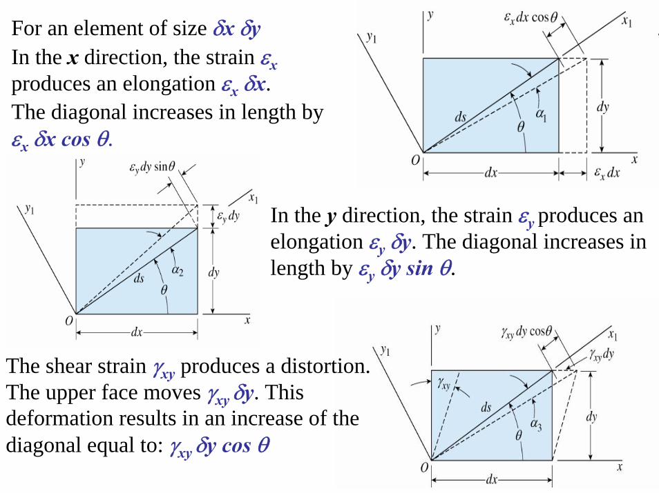
For an element of size δx δyIn the x direction, the strain εxproduces an elongation εx δx.The diagonal increases in length by εx δx cos θ.

In the y direction, the strain εy produces an elongation εy δy. The diagonal increases in length by εy δy sin θ.

The shear strain γxy produces a distortion. The upper face moves γxy δy. This deformation results in an increase of the diagonal equal to: γxy δy cos θ

The total increase Δd of the diagonal is the sum of the preceding three expressions, thus:

Δd = εx δx cos θ + εy δy sin θ + γxy δy cos θ

The normal strain εx1 in the x1 direction is equal to the increase in length divided by the initial length δs of the diagonal.

εx1 = Δd / ds = εx cos θ δx/δs + εy sin θ δy/δs + γxy cos θ δy/δs

Observing that δx/δs = cos θ and δy/δs = sin θ

θθγθεθεε

θθγθεθεε

cossin22

sincos

cossinsincos

221

221

⎟⎠⎞

⎜⎝⎛++=

++=

XYYXX

XYYXX

γ

Shear Strain γx1y1 associated with x1y1 axes.This strain is equal to the decrease in angle between lines in the material that were initially along the x1 and y1 axes. Oa and Ob were the lines initially along the x1 and y1 axis respectively. The deformation caused by the strains εx, εy and γxy caused the Oa and Ob lines to rotate and angle α and β from the x1 and y1 axis respectively. The shear strain γx1y1is the decrease in angle between the two lines that originally were at right angles, therefore, γx1y1 = α+β.

The angle α can be found from the deformations produced by the strains εx, εy and γxy . The strains εx and γxy produce a cw-rotation, while the strain εyproduces a ccw-rotation.

Let us denote the angle of rotation produced by εx , εy and γxy as α1 , α2 and α3 respectively. The angle α1 is equal to the distance εx δxsinθ divided by the length δs of the diagonal:α1 = εx sinθ dx/ds α2 = εy cosθ dy/ds α3 = γxy sinθ dy/dsObserving that dx/ds = cos θ and dy/ds = sin θ. The resulting ccw-rotation of the diagonal is

α = - α1 + α2 - α3 = - (εx – εy) sinθ cosθ - γxy sin2θ

The rotation of line Ob which initially was at at 90o to the line Oa can be found by substituting θ +90 for θ in the expression for α.

Because β is positive when clockwise. Thusβ = (εx – εy) sin(θ + 90) cos(θ + 90) + γxy sin2(θ +90) β = - (εx – εy) sinθ cosθ + γxy cos2θ

Adding α and β gives the shear strain γx1y1γx1y1 = α + β = - 2(εx – εy) sinθ cosθ + γxy (cos2θ - sin2θ)To put the equation in a more useful form:

( )θθγθθεθθεγ 2211 sincos2

cossincossin2

−++−= XYYX

YX

θθγθεθεε cossin22

sincos 221 ⎟

⎠⎞

⎜⎝⎛++= XY

YXX

θθγθεθεε cossin22

cossin 221 ⎟

⎠⎞

⎜⎝⎛−+= XY

YXY

( )⎥⎥⎥⎥⎥

⎦

⎤

⎢⎢⎢⎢⎢

⎣

⎡

⎥⎥⎥

⎦

⎤

⎢⎢⎢

⎣

⎡

−−−=

⎥⎥⎥⎥⎥

⎦

⎤

⎢⎢⎢⎢⎢

⎣

⎡

2sincoscossincossincossin2cossin

cossin2sincos

222

22

22

11

1

1

XY

Y

X

YX

Y

X

γεε

θθθθθθθθθθ

θθθθ

γεε

[ ]

[ ]

⎥⎥⎥⎥⎥

⎦

⎤

⎢⎢⎢⎢⎢

⎣

⎡

×=

⎥⎥⎥⎥⎥

⎦

⎤

⎢⎢⎢⎢⎢

⎣

⎡

⎥⎥⎥⎥⎥

⎦

⎤

⎢⎢⎢⎢⎢

⎣

⎡

×=

⎥⎥⎥⎥⎥

⎦

⎤

⎢⎢⎢⎢⎢

⎣

⎡

−

22

22

11

1

11

11

1

1

YX

Y

X

XY

Y

X

XY

Y

X

YX

Y

X

T

T

γεε

γεε

γεε

γεε [ ]

( )⎥⎥⎥

⎦

⎤

⎢⎢⎢

⎣

⎡

−−−=

θθθθθθθθθθ

θθθθ

22

22

22

sincoscossincossincossin2cossin

cossin2sincosT

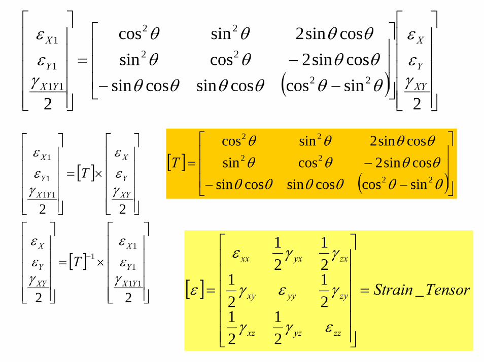
[ ] TensorStrain

zzyzxz

zyyyxy

zxyxxx

_

21

21

21

21

21

21

=

⎥⎥⎥⎥⎥⎥

⎦

⎤

⎢⎢⎢⎢⎢⎢

⎣

⎡

=

εγγ

γεγ

γγε

ε

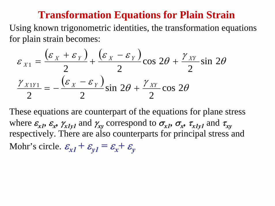
Transformation Equations for Plain StrainUsing known trigonometric identities, the transformation equations for plain strain becomes:

These equations are counterpart of the equations for plane stress where εx1, εx, γx1y1 and γxy correspond to σx1, σx, τx1y1 and τxyrespectively. There are also counterparts for principal stress and Mohr’s circle. εx1 + εy1 = εx+ εy

( ) ( )

( )θ

γθ

εεγ

θγ

θεεεε

ε

2cos2

2sin22

2sin2

2cos22

11

1

XYYXYX

XYYXYXX

+−

−=

+−

++

=

Principal Strains

The angle for the principal strains is

The value for the principal strains are

YX

XYP εε

γθ

−=2tan

( )

( ) 22

2

22

1

222

222

⎟⎠⎞

⎜⎝⎛+⎟

⎠⎞

⎜⎝⎛ −

−+

=

⎟⎠⎞

⎜⎝⎛+⎟

⎠⎞

⎜⎝⎛ −

++

=

XYYXYX

XYYXYX

γεεεεε

γεεεεε

Maximum ShearThe maximum shear strains in the xy plane are associated with axes at 45o to the directions of the principal strains:

( )

( )22

or 222

21

21

22

εεγ

εεγγεεγ

−=

−=⎟⎠⎞

⎜⎝⎛+⎟

⎠⎞

⎜⎝⎛ −

+=

MAX

MAXXYYXMAX

Mohr’s Circle for Plane Strain

ExampleAn element of material in plane strain undergoes the following strains: εx=340x10-6

εy=110x10-6

γxy=180x10-6

Determine the following: (a) the strains of an element oriented at an angle θ = 30o ; (b) the principal strains and (c) the maximum shear strains.

( ) ( )

( )θ

γθ

εεγ

θγ

θεεεε

ε

2cos2

2sin22

2sin2

2cos22

11

1

XYYXYX

XYYXYXX

+−

−=

+−

++

=Solution

Thenεx1 = 225x10-6 + (115x10-6) cos 60o + (90x10-6) sin 60o = 360x10-6

½ γx1y1 = - (115x10-6) (sin 60o ) + ( 90x10-6)(cos 60o) = - 55x10-6

Therefore γx1y1 = - 110x10-6

The strain εy1 can be obtained from the equation εx1 + εy1 = εx+ εyεy1 = (340 + 110 -360)10-6 = 90x10-6

( )

( ) 22

2

22

1

222

222

⎟⎠⎞

⎜⎝⎛+⎟

⎠⎞

⎜⎝⎛ −

−+

=

⎟⎠⎞

⎜⎝⎛+⎟

⎠⎞

⎜⎝⎛ −

++

=

XYYXYX

XYYXYX

γεεεεε

γεεεεε

(b) Principal StrainsThe principal strains are readily determine from the following equations:ε1 = 370x10-6 ε2 = 80x10-6

(c) Maximum Shear StrainThe maximum shear strain is calculated from the equation:½ γmax = SQR[((εx – εy)/2)2 + ( ½ γxy)2] or γmax = (ε1 – ε2 ) Then γmax = 290x10-6

The normal strains of this element is εaver = ½ (εx + εy) = 225x10-6

For 3-D problems

[ ]

⎥⎥⎥⎥⎥⎥

⎦

⎤

⎢⎢⎢⎢⎢⎢

⎣

⎡

=

zzyzx

yzyyx

xzxyx

εγγ

γεγ

γγε

ε

21

21

21

21

21

21

Which is a symmetrical matrix. As in the case of stresses:

0

21

21

21

21

21

21

000

21

21

21

21

21

21

=

−

−

−

⎥⎥⎥

⎦

⎤

⎢⎢⎢

⎣

⎡=

⎥⎥⎥

⎦

⎤

⎢⎢⎢

⎣

⎡

⎥⎥⎥⎥⎥⎥

⎦

⎤

⎢⎢⎢⎢⎢⎢

⎣

⎡

−

−

−

εεγγ

γεεγ

γγεε

εεγγ

γεεγ

γγεε

zzyzx

yzyyx

xzxyx

zzyzx

yzyyx

xzxyx

mlk

321 εεε ⟩⟩

Dilatation (Volume strain)Under pressure: the volume will change

p

pp

p

V-ΔVzyxVV εεε ++=

Δ=Δ

222

3

222

2

1

322

13

2222222

222

0

⎟⎟⎠

⎞⎜⎜⎝

⎛⋅−⎟

⎠⎞

⎜⎝⎛⋅−⎟⎟

⎠

⎞⎜⎜⎝

⎛⋅−⎟⎟

⎠

⎞⎜⎜⎝

⎛⋅⎟

⎠⎞

⎜⎝⎛⋅⎟⎟

⎠

⎞⎜⎜⎝

⎛⋅+⋅⋅=

⎟⎟⎠

⎞⎜⎜⎝

⎛−⎟

⎠⎞

⎜⎝⎛−⎟⎟

⎠

⎞⎜⎜⎝

⎛−⋅+⋅+⋅=

++==−⋅+⋅−

xyz

xzy

yzx

yzxzxyzyx

yzxzxyzxzyyx

zyx

I

I

IIII

γεγε

γε

γγγεεε

γγγεεεεεε

εεεεεε

Strain Deviator33

zyx εεε ++=

ΔMean strain

It produces a volume change (not a shape change)

[ ]

⎥⎥⎥⎥⎥⎥

⎦

⎤

⎢⎢⎢⎢⎢⎢

⎣

⎡

Δ−

Δ−

Δ−

=

31

21

21

21

31

21

21

21

31

zzyzx

yzyyx

xzxyx

D

εγγ

γεγ

γγε

ε

[ ]

Strain Deviator Matrix

⎥⎥⎥⎥⎥⎥

⎦

⎤

⎢⎢⎢⎢⎢⎢

⎣

⎡

Δ−

Δ−

Δ−

=

3100

0310

0031

3

2

1

ε

ε

ε

εD

Application : Strain Gauge and Strain Rosette

(Hooke’s Law)When strains are small, most of materials are

linear elastic. Tensile: σ = Ε ε

Shear: τ = G γ

Poisson’s ratio

Nominal lateral strain (transverse strain)z

zz l

l

0

Δ=ε

x

xx l

l

0

Δ−=ε

Poisson’s ratio:z

x

straintensilestrainlateral

εεν −=−=

Relationships between Stress and Strain

Relationships between Stress and Strain

For isotropic materials

Elastic Stress-Strain Relationships

00

3

2

11

===

σσ

εσ EPrincipal Stresses Principal Strains

E

E

E

13

12

11

σνε

σνε

σε

−=

−=

=Uniaxial

An isotropic material has a stress-strain relationships that are independent of the orientation of the coordinate system at a point. A material is said to be homogenous if the material properties are the same at all points in the body

[ ]

⎪⎪⎪⎪

⎭

⎪⎪⎪⎪

⎬

⎫

⎪⎪⎪⎪

⎩

⎪⎪⎪⎪

⎨

⎧

=

xy

zx

yz

z

y

x

τττσσσ

σ

[ ]

⎪⎪⎪⎪

⎭

⎪⎪⎪⎪

⎬

⎫

⎪⎪⎪⎪

⎩

⎪⎪⎪⎪

⎨

⎧

=

xy

zx

yz

z

y

x

γγγεεε

ε

[ ]

⎪⎪⎪⎪

⎭

⎪⎪⎪⎪

⎬

⎫

⎪⎪⎪⎪

⎩

⎪⎪⎪⎪

⎨

⎧

=

00000

xσ

σ

xx E εσ =

EEEx

zx

yx

xσνεσνεσε −=−==

[ ]

⎪⎪⎪⎪

⎭

⎪⎪⎪⎪

⎬

⎫

⎪⎪⎪⎪

⎩

⎪⎪⎪⎪

⎨

⎧

=

000

z

y

x

εεε

ε⎪⎪⎪⎪

⎭

⎪⎪⎪⎪

⎬

⎫

⎪⎪⎪⎪

⎩

⎪⎪⎪⎪

⎨

⎧

⎥⎥⎥⎥⎥⎥⎥⎥⎥⎥⎥⎥⎥

⎦

⎤

⎢⎢⎢⎢⎢⎢⎢⎢⎢⎢⎢⎢⎢

⎣

⎡

−−

−−

−−

=

⎪⎪⎪⎪

⎭

⎪⎪⎪⎪

⎬

⎫

⎪⎪⎪⎪

⎩

⎪⎪⎪⎪

⎨

⎧

00000

100000

010000

001000

0001

0001

0001

000

x

z

y

x

G

G

G

EEE

EEE

EEEσ

υυ

υυ

υυ

εεε

Uniaxial Stresses

( )

( )

01

1

3

212

2

221

1

=+

+=

++

=

σν

νεεσ

ννεεσ

E

E

Principal Stresses Principal Strains

EE

EE

EE

213

122

211

σνσνε

σνσε

σνσε

−−=

−=

−=Biaxial

( ) ( )

( ) ( )

( ) ( )2

2133

2312

2

2321

1

211

211

211

ννεεννεσ

ννεεννεσ

ννεεννεσ

−−++−

=

−−++−

=

−−++−

=

E

E

E

Principal Stresses Principal Strains

EEE

EEE

EEE

2133

3122

3211

σνσνσε

σνσνσε

σνσνσε

−−=

−−=

−−=

Triaxial

[ ]

⎪⎪⎪⎪

⎭

⎪⎪⎪⎪

⎬

⎫

⎪⎪⎪⎪

⎩

⎪⎪⎪⎪

⎨

⎧

=

xy

zx

yz

z

y

x

τττσσσ

σ

[ ]

⎪⎪⎪⎪

⎭

⎪⎪⎪⎪

⎬

⎫

⎪⎪⎪⎪

⎩

⎪⎪⎪⎪

⎨

⎧

=

xy

zx

yz

z

y

x

γγγεεε

ε

1

1

1

zyxz

zyxy

zyxx

EEE

EEE

EEE

σσνσνε

σνσσνε

σνσνσε

+−−=

−+−=

−−=

[ ]

⎪⎪⎪⎪

⎭

⎪⎪⎪⎪

⎬

⎫

⎪⎪⎪⎪

⎩

⎪⎪⎪⎪

⎨

⎧

=

000

z

y

x

εεε

ε

⎪⎪⎪⎪

⎭

⎪⎪⎪⎪

⎬

⎫

⎪⎪⎪⎪

⎩

⎪⎪⎪⎪

⎨

⎧

⎥⎥⎥⎥⎥⎥⎥⎥⎥⎥⎥⎥⎥

⎦

⎤

⎢⎢⎢⎢⎢⎢⎢⎢⎢⎢⎢⎢⎢

⎣

⎡

−−

−−

−−

=

⎪⎪⎪⎪

⎭

⎪⎪⎪⎪

⎬

⎫

⎪⎪⎪⎪

⎩

⎪⎪⎪⎪

⎨

⎧

000

100000

010000

001000

0001

0001

0001

000

z

y

x

z

y

x

G

G

G

EEE

EEE

EEE

σσσ

υυ

υυ

υυ

εεε

[ ]

⎪⎪⎪⎪

⎭

⎪⎪⎪⎪

⎬

⎫

⎪⎪⎪⎪

⎩

⎪⎪⎪⎪

⎨

⎧

=

000

z

y

x

σσσ

σ

Triaxial Stresses

For an isotropic material, the principal axes for stress and theprincipal axes for strain coincide.

YX

XY

εεγθε −

=2tan

( )( )

G

Exy

xy

yxyx

τγ

σσνεε

=

−−=− 11

( )( ) ( ) ( ) σε θσσ

τνσσν

τ

εεγθ 2tan

212112tan =

−⋅

−=

−−=

−=

yx

xy

yx

xy

YX

XY

GE

E

G

Plane Stress ( )

( )

G

E

E

xyxy

xyy

yxx

τγ

νσσε

νσσε

=

−=

−=

1

1 ( )

0

0

=

=

+−=

zx

yz

yxz E

γ

γ

σσνε

Plane Strain

( )( ) ( )[ ]

( )( ) ( )[ ]

xyxy

xyy

yxx

G

E

E

γτ

νεεννν

σ

νεεννν

σ

=

+−−+

=

+−−+

=

1211

1211 ( )( ) ( )

0

0211

=

=

+−+

=

xz

yz

yxzE

τ

τ

εενν

νσ

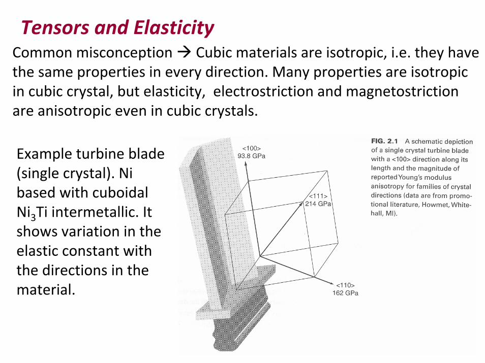
Tensors and ElasticityCommon misconception  Cubic materials are isotropic, i.e. they have the same properties in every direction. Many properties are isotropic in cubic crystal, but elasticity,  electrostriction and magnetostrictionare anisotropic even in cubic crystals.

Example turbine blade (single crystal). Ni based with cuboidalNi3Ti intermetallic. It shows variation in the elastic constant with the directions in the material. 

Some polycrystalline materials develop preferred orientations during processing. They will show a degree of anisotropy that is dependent on the degree of preferred orientation or texture.

Tensor: A specific type of matrix representation that can relate the directionality of either a material property (property tensors –conductivity, elasticity) or a condition/state (condition tensors – stress, strain).

Tensor of zero‐rank: scalar quantity (density, temperature).Tensor of first‐rank: vector quantity (force, electric field, flux of atoms).Tensor of second‐rank: relates two vector quantities (flux of atoms with concentration gradient).

Tensor third‐rank: relates vector with a second rank tensor (electric field with strain in a piezoelectric material)

Tensor Fourth‐rank: relates two second rank tensors (relates strain and stress – Elasticity)  

The key to understanding property or condition tensors is to recognize that tensors can be specified with reference to some coordinate system which is usually defined in 3‐D space by orthogonal axes that obey a right‐hand rule.

Rotation Matrix and Euler Angles:Rotation Matrix and Euler Angles: Several schemes can be used to produce a rotation matrix. The three Euler angles are given as three counterclockwise rotations: 

(a)A rotation about a z‐axis, defined as φ1 (b)A rotation about the new x‐axis, defined as Φ(c)A rotation about the second z‐position, defined as φ2

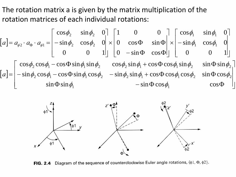
The rotation matrix a is given by the matrix multiplication of the rotation matrices of each individual rotations:

[ ]

[ ]⎥⎥⎥

⎦

⎤

⎢⎢⎢

⎣

⎡

ΦΦ−ΦΦΦ+−Φ−−ΦΦ+Φ−

=

⎥⎥⎥

⎦

⎤

⎢⎢⎢

⎣

⎡−×

⎥⎥⎥

⎦

⎤

⎢⎢⎢

⎣

⎡

ΦΦ−ΦΦ×

⎥⎥⎥

⎦

⎤

⎢⎢⎢

⎣

⎡−=⋅⋅= Φ

coscossinsinsincossincoscoscossinsincossincoscossinsinsinsincoscossincossinsincoscoscos

1000cossin0sincos

cossin0sincos0

001

1000cossin0sincos

11

221122112

221122112

11

11

22

22

12

φφφφφφφφφφφφφφφφφφφφ

φφφφ

φφφφ

φφ

a

aaaa

Stereographic Projection

Crystallographic directions, plane normals and planes can be all represented in the stereographic projection.

Locating a pole in a stereographic projection:

o

o

o

5.74141

1 3 2 1 0 0cos

7.36141

1 3 2 0 1 0cos

6.57141

1 3 2 0 0 1cos

1 3 2

1-

1-

1-

=⎥⎦

⎤⎢⎣

⎡ ⋅

=⎥⎦

⎤⎢⎣

⎡ ⋅

=⎥⎦

⎤⎢⎣

⎡ ⋅

Find the angle of the pole with the three axes:

ExampleThe relationship between orientation and applied stress is important in describing the mechanical performance of many crystalline metals and composites.The relationship between applied stress and crystal direction isessential in interpreting the microscopic deformation mechanismsoperating in deforming crystals.

[ ]⎥⎥⎥

⎦

⎤

⎢⎢⎢

⎣

⎡

−=

100030002

TConsider a property‐tensor or a condition tensor Tin the original {x y z} axes given by:  

Find the tensor T’ , for the rotation shown below from the initial [100], [010], [001] axes of a cubic crystal

o

o

o

07.54

45

2

1

=

=Φ

=

φ

φ [ ]

⎥⎥⎥

⎦

⎤

⎢⎢⎢

⎣

⎡

−+−=

⎥⎥⎥

⎦

⎤

⎢⎢⎢

⎣

⎡

−+−−−+−

=

⎥⎥⎥

⎦

⎤

⎢⎢⎢

⎣

⎡

ΦΦ−ΦΦΦ+−Φ−−ΦΦ+Φ−

=

7.54cos45cos7.54sin45sin7.54sin7.54sin45cos7.54cos45sin7.54cos

045sin45cos][

7.54cos45cos7.54sin45sin7.54sin0cos7.54sin0cos45cos7.54cos45sin0sin0cos45sin7.54cos45cos0sin0sin7.54sin0sin45cos7.54cos45sin0cos0sin45sin7.54cos45cos0cos

][

coscossinsinsincossincoscoscossinsincossincoscossinsinsinsincoscossincossinsincoscoscos

11

221122112

221122112

a

a

aφφ

φφφφφφφφφφφφφφφφφφ

⎥⎥⎥⎥⎥⎥

⎦

⎤

⎢⎢⎢⎢⎢⎢

⎣

⎡

−

−=

31

31

31

62

61

61

02

12

1

][a

[ ] [ ]TaTaT ××='

⎥⎥⎥

⎦

⎤

⎢⎢⎢

⎣

⎡

−−−

−=

⎥⎥⎥⎥⎥⎥

⎦

⎤

⎢⎢⎢⎢⎢⎢

⎣

⎡

−

−

×⎥⎥⎥

⎦

⎤

⎢⎢⎢

⎣

⎡

−×

⎥⎥⎥⎥⎥⎥

⎦

⎤

⎢⎢⎢⎢⎢⎢

⎣

⎡

−

−=33.165.1408.065.1167.0289.0408.0289.05.2

31

620

31

61

21

31

61

21

100030002

31

31

31

62

61

61

02

12

1

]'[T

EEE

EEE

EEE

zyxz

zyxy

zyxx

σσνσνε

σνσσνε

σνσ

νσε

+−−=

−+−=

−−=

1

1

1

xyxy

zxzx

yzyz

G

G

G

τγ

τγ

τγ

=

=

=

Isotropic Materials

⎪⎪⎪⎪

⎭

⎪⎪⎪⎪

⎬

⎫

⎪⎪⎪⎪

⎩

⎪⎪⎪⎪

⎨

⎧

⎥⎥⎥⎥⎥⎥⎥⎥

⎦

⎤

⎢⎢⎢⎢⎢⎢⎢⎢

⎣

⎡

=

⎪⎪⎪⎪

⎭

⎪⎪⎪⎪

⎬

⎫

⎪⎪⎪⎪

⎩

⎪⎪⎪⎪

⎨

⎧

xy

zx

yz

z

y

x

xy

zx

yz

z

y

x

SSSSSSSSSSSSSSSSSSSSSSSSSSSSSSSSSSSS

τττσσσ

γγγεεε

666564636261

565554535251

464544434241

363534333231

262524232221

161514131211

xyzxyzzyxx SSSSSS τττσσσε 161514131211 +++++=

xyzxyzzyxy SSSSSS τττσσσε 262524232221 +++++=

xyzxyzzyxz SSSSSS τττσσσε 363534333231 +++++=

xyzxyzzyxyz SSSSSS τττσσσγ 464544434241 +++++=

xyzxyzzyxzx SSSSSS τττσσσγ 565554535251 +++++=

xyzxyzzyxxy SSSSSS τττσσσγ 666564636261 +++++=

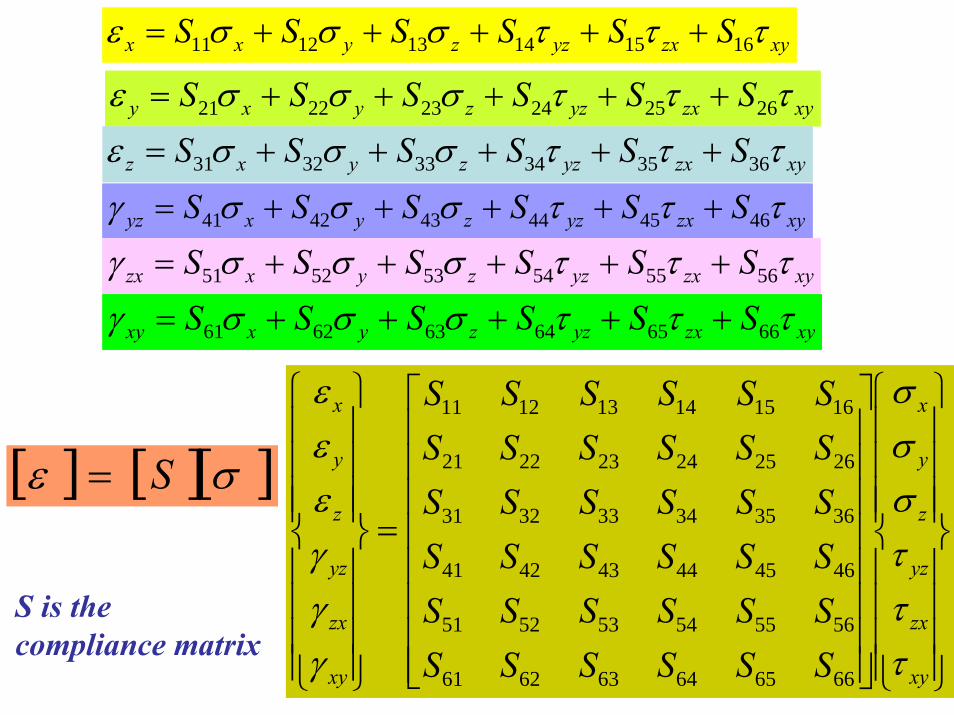
[ ] [ ][ ]σε S=

S is the compliance matrix

Isotropic MaterialsAn isotropic material has stress-strain relationships that are independent of the orientation of the coordinate system at a point.

The isotropic material requires only two independent material constants, namely the Elastic Modulus and the Poisson’s Ratio.

⎪⎪⎪⎪

⎭

⎪⎪⎪⎪

⎬

⎫

⎪⎪⎪⎪

⎩

⎪⎪⎪⎪

⎨

⎧

⎥⎥⎥⎥⎥⎥⎥⎥⎥⎥⎥⎥⎥

⎦

⎤

⎢⎢⎢⎢⎢⎢⎢⎢⎢⎢⎢⎢⎢

⎣

⎡

−−

−−

−−

=

⎪⎪⎪⎪

⎭

⎪⎪⎪⎪

⎬

⎫

⎪⎪⎪⎪

⎩

⎪⎪⎪⎪

⎨

⎧

xy

zx

yz

z

y

x

xy

zx

yz

z

y

x

G

G

G

EEE

EEE

EEE

τττσσσ

νν

νν

νν

γγγεεε

100000

010000

001000

0001

0001

0001

( )( )( ) ( )( ) ( )( )

( )( )( )

( )( ) ( )( )

( )( ) ( )( )( )

( )( )

⎪⎪⎪⎪

⎭

⎪⎪⎪⎪

⎬

⎫

⎪⎪⎪⎪

⎩

⎪⎪⎪⎪

⎨

⎧

⎥⎥⎥⎥⎥⎥⎥⎥⎥⎥⎥

⎦

⎤

⎢⎢⎢⎢⎢⎢⎢⎢⎢⎢⎢

⎣

⎡

−+−

−+−+

−+−+−

−+

−+−+−+−

=

⎪⎪⎪⎪

⎭

⎪⎪⎪⎪

⎬

⎫

⎪⎪⎪⎪

⎩

⎪⎪⎪⎪

⎨

⎧

xy

zx

yz

z

y

x

xy

zx

yz

z

y

x

GG

G

EEE

EEE

EEE

γγγεεε

ννν

ννν

ννν

ννν

ννν

ννν

ννν

ννν

ννν

τττσσσ

000000000000000

000211

1211211

000211211

1211

000211211211

1

[ ] [ ][ ]εσ C=

C is the elastic or stiffness matrix

The isotropic material requires only two independent material constants, namely the Elastic Modulus and the Poisson’s Ratio.

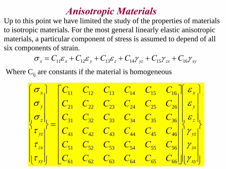
Anisotropic MaterialsUp to this point we have limited the study of the properties of materials to isotropic materials. For the most general linearly elastic anisotropic materials, a particular component of stress is assumed to depend of all six components of strain.

xyzxyzzyxx CCCCCC γγγεεεσ 161514131211 +++++=

Where Cij are constants if the material is homogeneous

⎪⎪⎪⎪

⎭

⎪⎪⎪⎪

⎬

⎫

⎪⎪⎪⎪

⎩

⎪⎪⎪⎪

⎨

⎧

⎥⎥⎥⎥⎥⎥⎥⎥

⎦

⎤

⎢⎢⎢⎢⎢⎢⎢⎢

⎣

⎡

=

⎪⎪⎪⎪

⎭

⎪⎪⎪⎪

⎬

⎫

⎪⎪⎪⎪

⎩

⎪⎪⎪⎪

⎨

⎧

xy

zx

yz

z

y

x

xy

zx

yz

z

y

x

CCCCCCCCCCCCCCCCCCCCCCCCCCCCCCCCCCCC

γγγεεε

τττσσσ

666564636261

565554535251

464544434241

363534333231

262524232221

161514131211

⎪⎪⎪⎪

⎭

⎪⎪⎪⎪

⎬

⎫

⎪⎪⎪⎪

⎩

⎪⎪⎪⎪

⎨

⎧

⎥⎥⎥⎥⎥⎥⎥⎥

⎦

⎤

⎢⎢⎢⎢⎢⎢⎢⎢

⎣

⎡

=

⎪⎪⎪⎪

⎭

⎪⎪⎪⎪

⎬

⎫

⎪⎪⎪⎪

⎩

⎪⎪⎪⎪

⎨

⎧

xy

zx

yz

z

y

x

xy

zx

yz

z

y

x

CCCCCCCCCCCCCCCCCCCCCCCCCCCCCCCCCCCC

γγγεεε

τττσσσ

665646362616

565545352515

464544342414

363534332313

262524232212

161514131211

Taking energy considerations the coefficients of this matrix aresymmetric. Hence, instead of 36 independent constant, we have 21 independent constants

[ ]

⎥⎥⎥⎥⎥⎥⎥⎥

⎦

⎤

⎢⎢⎢⎢⎢⎢⎢⎢

⎣

⎡

=

665646362616

565545352515

464544342414

363534332313

262524232212

161514131211

CCCCCCCCCCCCCCCCCCCCCCCCCCCCCCCCCCCC

C

C is referred to as the elastic matrix or stiffness matrix.

[ ] [ ][ ]

⎪⎪⎪⎪

⎭

⎪⎪⎪⎪

⎬

⎫

⎪⎪⎪⎪

⎩

⎪⎪⎪⎪

⎨

⎧

⎥⎥⎥⎥⎥⎥⎥⎥

⎦

⎤

⎢⎢⎢⎢⎢⎢⎢⎢

⎣

⎡

=

⎪⎪⎪⎪

⎭

⎪⎪⎪⎪

⎬

⎫

⎪⎪⎪⎪

⎩

⎪⎪⎪⎪

⎨

⎧

=

xy

zx

yz

z

y

x

xy

zx

yz

z

y

x

SSSSSSSSSSSSSSSSSSSSSSSSSSSSSSSSSSSS

S

τττσσσ

γγγεεε

σε

665646362616

565545352515

464544342414

363534332313

262524232212

161514131211

Hence, we can also write

The matrix S is referred to as the compliance matrix and the elements of S are the compliances.

21 elastic constants are required to describe the most general anisotropic material (fully anisotropic). This is in contrast to an isotropic material for which there are only two independent elastic constants (typically the Young Modulus and the Poisson’s ratio).

( )( )( ) ( )( )

( )( ) ( )[ ])εεE

)εεEE

zyxx

zyxx

++−−+

=

+−+

+−+

−=

(1211

(211211

1

νεννν

σ

νννε

νννσ

Many materials of practical interest contain certain material symmetries with respect to their elastic properties (elastic symmetries). Other type of symmetries are possible optical, electrical and thermal properties.

Let us determine the structure of the elastic matrix for a material with a single plane of elastic symmetry. Crystals whose crystalline structure is monoclinic as examples of materials possessing a single plane of elastic symmetry. Example Iron aluminide, gypsum, talc, ice, selenium

Materials with one plane of symmetry are referred to as Monoclinic materials.

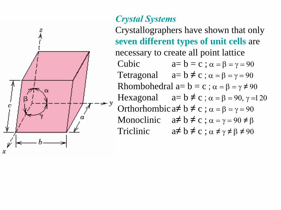
Crystal SystemsCrystallographers have shown that only seven different types of unit cells are necessary to create all point latticeCubic a= b = c ; α = β = γ = 90Tetragonal a= b ≠ c ; α = β = γ = 90Rhombohedral a= b = c ; α = β = γ ≠ 90Hexagonal a= b ≠ c ; α = β = 90, γ =120Orthorhombica≠ b ≠ c ; α = β = γ = 90Monoclinic a≠ b ≠ c ; α = γ = 90 ≠ β Triclinic a≠ b ≠ c ; α ≠ γ ≠ β ≠ 90

Monoclinic MaterialsLet us assume that the z-plane is the plane of elastic symmetry.For such a material the elastic coefficients in the stress-strain law must remain unchanged when subjected to a transformation that represents a reflection in the symmetry plane. For monoclinic materials (due to one plane of elastic symmetry) the number of independent elastic constants is reduced from 21 to 13.

⎪⎪⎪⎪

⎭

⎪⎪⎪⎪

⎬

⎫

⎪⎪⎪⎪

⎩

⎪⎪⎪⎪

⎨

⎧

⎥⎥⎥⎥⎥⎥⎥⎥

⎦

⎤

⎢⎢⎢⎢⎢⎢⎢⎢

⎣

⎡

=

⎪⎪⎪⎪

⎭

⎪⎪⎪⎪

⎬

⎫

⎪⎪⎪⎪

⎩

⎪⎪⎪⎪

⎨

⎧

xy

zx

yz

z

y

x

xy

zx

yz

z

y

x

CCCCCCCC

CCCCCCCCCCCC

γγγεεε

τττσσσ

66362616

5545

4544

36332313

26232212

16131211

0000000000

000000

KEY TO NOTATION

TRICLINIC (21)

MONOCLINIC (13)

ORTHORHOMBIC (9) CUBIC (3)

(7) TETRAGONAL (6)

HEXAGONAL (5) ISOTROPIC (2)

(7) TRIGONAL (6)

Orthotropic MaterialsLet us consider a material with a second plane of elastic symmetry. The y-plane and the z-plane are the planes of elastic symmetry and are perpendicular to each other. Again, for such a material the elastic coefficients in the stress-strain law must remain unchanged when subjected to a transformation that represents a reflection in the symmetry plane. For orthotropic materials (due to the two planes of elastic symmetry) the number of independent elastic constants isreduced from 21 to 9.

⎪⎪⎪⎪

⎭

⎪⎪⎪⎪

⎬

⎫

⎪⎪⎪⎪

⎩

⎪⎪⎪⎪

⎨

⎧

⎥⎥⎥⎥⎥⎥⎥⎥

⎦

⎤

⎢⎢⎢⎢⎢⎢⎢⎢

⎣

⎡

=

⎪⎪⎪⎪

⎭

⎪⎪⎪⎪

⎬

⎫

⎪⎪⎪⎪

⎩

⎪⎪⎪⎪

⎨

⎧

xy

zx

yz

z

y

x

xy

zx

yz

z

y

x

CC

CCCCCCCCCC

γγγεεε

τττσσσ

66

55

44

332313

232212

131211

000000000000000000000000

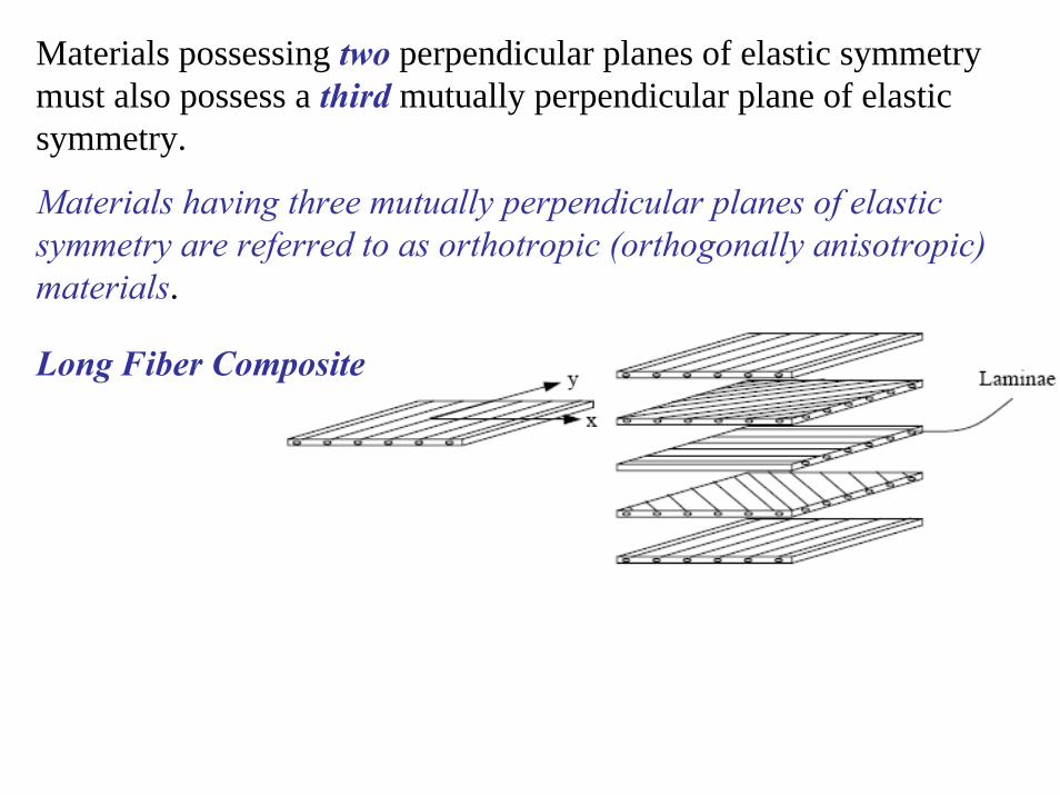
Materials possessing two perpendicular planes of elastic symmetry must also possess a third mutually perpendicular plane of elastic symmetry.

Materials having three mutually perpendicular planes of elastic symmetry are referred to as orthotropic (orthogonally anisotropic) materials.

Long Fiber Composite

Transversely Isotropic MaterialsMaterials that are isotropic in a plane.Transversely isotropic materials require five independent material constants.

( )⎪⎪⎪⎪

⎭

⎪⎪⎪⎪

⎬

⎫

⎪⎪⎪⎪

⎩

⎪⎪⎪⎪

⎨

⎧

⎥⎥⎥⎥⎥⎥⎥⎥

⎦

⎤

⎢⎢⎢⎢⎢⎢⎢⎢

⎣

⎡

−

=

⎪⎪⎪⎪

⎭

⎪⎪⎪⎪

⎬

⎫

⎪⎪⎪⎪

⎩

⎪⎪⎪⎪

⎨

⎧

xy

zx

yz

z

y

x

xy

zx

yz

z

y

x

CCC

CCCCCCCCCC

γγγεεε

τττσσσ

200000

0000000000000000000

1211

44

44

331313

131112

131211

Isotropic MaterialsThe isotropic material requires only two independent material constants, namely the Elastic Modulus and the Poisson’s Ratio.

( )

( )

( ) ⎪⎪⎪⎪

⎭

⎪⎪⎪⎪

⎬

⎫

⎪⎪⎪⎪

⎩

⎪⎪⎪⎪

⎨

⎧

⎥⎥⎥⎥⎥⎥⎥⎥⎥⎥

⎦

⎤

⎢⎢⎢⎢⎢⎢⎢⎢⎢⎢

⎣

⎡

−

−

−=

⎪⎪⎪⎪

⎭

⎪⎪⎪⎪

⎬

⎫

⎪⎪⎪⎪

⎩

⎪⎪⎪⎪

⎨

⎧

xy

zx

yz

z

y

x

xy

zx

yz

z

y

x

CC

CC

CCCCCCCCCCC

γγγεεε

τττσσσ

200000

02

0000

002

000

000000000

1211

1211

1211

111212

121112

121211

( )( )( ) ( )( )

( )( ) GECCECEC =

+=

−−+

=−+

−=

νννν

ννν

122

211

2111 1211

1211

Engineering Material Constants for Orthotropic Materials

The quantities appearing in the coefficient matrix can be written in terms of well understood engineering constants such as the Young Modulus and the Poisson’s ratio. For the x, y and z coordinate axes we can write:

zzz

yyy

xxx

E

EE

εσ

εσεσ

=

==

Where the Young Modulus in the x-, y- and z-directions are not necessarily equal.

Any extension in the x-axis is accompanied by a contraction in the y- and z- axis. However, this quantities are not necessarily equal in orthotropic materials.

Where νxy is the contraction in the y-direction due to the stress in the x-direction

xxzz

xxyy

ενε

ενε

−=

−=

If all three stresses are applied simultaneously, then:

zz

yy

yzx

x

xzy

zz

zyy

yx

x

xyy

zz

zxy

y

yxx

xx

EEE

EEE

EEE

σσν

σνε

σν

σσν

ε

σνσν

σε

1

1

1

+−−=

−+−=

−−=

[ ] [ ][ ]

⎪⎪⎪⎪

⎭

⎪⎪⎪⎪

⎬

⎫

⎪⎪⎪⎪

⎩

⎪⎪⎪⎪

⎨

⎧

⎥⎥⎥⎥⎥⎥⎥⎥

⎦

⎤

⎢⎢⎢⎢⎢⎢⎢⎢

⎣

⎡

=

⎪⎪⎪⎪

⎭

⎪⎪⎪⎪

⎬

⎫

⎪⎪⎪⎪

⎩

⎪⎪⎪⎪

⎨

⎧

=

xy

zx

yz

z

y

x

xy

zx

yz

z

y

x

SS

SSSSSSSSSS

S

τττσσσ

γγγεεε

σε

66

55

44

332313

232212

131211

000000000000000000000000

Comparing with the compliance matrix for orthotropic materials:

1 1 1

231312

332211

y

yz

z

zy

x

xz

z

zx

x

xy

y

yx

zyx

EES

EES

EES

ES

ES

ES

νννννν−=−=−=−=−=−=

===

Where νxy is the contraction in the y-direction due to the stress in the x-direction

Whereas with isotropic materials the relationship between shear stress and shear strain is the same in any coordinate planes, for orthotropic materials these relationships are not the same.

1 1 1

1 1 1

665544xyzxyz

zxzx

zxyzyz

yzxyxy

xy

GS

GS

GS

GGG

===

=== τγτγτγ

⎪⎪⎪⎪

⎭

⎪⎪⎪⎪

⎬

⎫

⎪⎪⎪⎪

⎩

⎪⎪⎪⎪

⎨

⎧

⎥⎥⎥⎥⎥⎥⎥⎥⎥⎥⎥⎥⎥⎥⎥⎥

⎦

⎤

⎢⎢⎢⎢⎢⎢⎢⎢⎢⎢⎢⎢⎢⎢⎢⎢

⎣

⎡

−−

−−

−−

=

⎪⎪⎪⎪

⎭

⎪⎪⎪⎪

⎬

⎫

⎪⎪⎪⎪

⎩

⎪⎪⎪⎪

⎨

⎧

xy

zx

yz

z

y

x

xy

zx

yz

zy

yz

x

xz

z

zy

yx

xy

z

zx

y

yx

x

xy

zx

yz

z

y

x

G

G

G

EEE

EEE

EEE

τττσσσ

νν

νν

νν

γγγεεε

100000

010000

001000

0001

0001

0001

⎪⎪⎪⎪

⎭

⎪⎪⎪⎪

⎬

⎫

⎪⎪⎪⎪

⎩

⎪⎪⎪⎪

⎨

⎧

⎥⎥⎥⎥⎥⎥⎥⎥⎥⎥⎥⎥

⎦

⎤

⎢⎢⎢⎢⎢⎢⎢⎢⎢⎢⎢⎢

⎣

⎡

Δ−

Δ+

Δ+

Δ+

Δ−

Δ+

Δ+

Δ+

Δ−

=

⎪⎪⎪⎪

⎭

⎪⎪⎪⎪

⎬

⎫

⎪⎪⎪⎪

⎩

⎪⎪⎪⎪

⎨

⎧

xy

zx

yz

z

y

x

xy

zx

yz

yx

yxxy

yx

yxxzyz

yx

yzxyxz

zx

xyzxzy

zx

xzzx

zx

zyxzxy

zy

zyyxzx

zy

yzzxyx

zy

zyyz

xy

zx

yz

z

y

x

GG

GEEEEEE

EEEEEE

EEEEEE

γγγεεε

νννννννν

νννννννν

νννννννν

τττσσσ

000000000000000

0001

0001

0001

zyx

zxyzxyxzzxzyyzyxxy

EEEννννννννν 21 −−−−

=Δ

⎪⎭

⎪⎬

⎫

⎪⎩

⎪⎨

⎧

⎥⎥⎥⎥⎥⎥⎥

⎦

⎤

⎢⎢⎢⎢⎢⎢⎢

⎣

⎡

−

−

=⎪⎭

⎪⎬

⎫

⎪⎩

⎪⎨

⎧

xy

y

x

xy

yx

xy

y

yx

x

xy

y

x

G

EE

EE

τσσ

ν

ν

γεε

100

01

01

⎪⎭

⎪⎬

⎫

⎪⎩

⎪⎨

⎧

⎥⎥⎥

⎦

⎤

⎢⎢⎢

⎣

⎡=

⎪⎭

⎪⎬

⎫

⎪⎩

⎪⎨

⎧

xy

y

x

xy

y

x

CCCCC

γεε

τσσ

33

2212

1211

0000

In 2-D

⎪⎭

⎪⎬

⎫

⎪⎩

⎪⎨

⎧

⎥⎥⎥⎥⎥⎥⎥

⎦

⎤

⎢⎢⎢⎢⎢⎢⎢

⎣

⎡

−−

−−

=⎪⎭

⎪⎬

⎫

⎪⎩

⎪⎨

⎧

xy

y

x

xy

yxxy

y

yxxy

yxy

yxxy

xyx

yxxy

x

xy

y

x

G

EE

EE

γεε

ννννν

ννν

νν

τσσ

00

011

011

Neumann’s PrincipleThis is the most important concept in crystal physics. It states; ……………... the symmetry of any physical property of a crystal must include the symmetry elements of the point group of the crystal. This means that measurements made in symmetry‐related directions will give the same property coefficients.

Example: NaCl belongs to the m3m group . The [100] and [010] directions are equivalent.

Since these directions are physically the same, it should be expected that measurements of permittivity, elasticity or any other physical property will be the same in these two directions.

Crystal System External Minimum Symmetry Unit Cell Properties

Triclinic None a, b, c, al, be, ga,Monoclinic One 2‐fold axis, || to b (b unique)  a, b, c, 90, be, 90Orthorhombic Three perpendicular 2‐folds a, b, c, 90, 90, 90Tetragonal One 4‐fold axis, parallel c a, a, c, 90, 90, 90Trigonal One 3‐fold axis a, a, c, 90, 90, 120Hexagonal One 6‐fold axis a, a, c, 90, 90, 120Cubic Four 3‐folds along space diagonal a, a, ,a, 90, 90, 90

7 Crystal Systems

triclinictrigonal

hexagonal

cubic tetragonalmonoclinic

orthorhombic

Anisotropy Factor

Cubic SymmetryFor cubic crystals, there are four three‐fold symmetry axes (along the <111> body diagonals) such that: 

665544

312312

332211

SSSSSSSSS

======

There is a reduction of the nine constants for orthotropic symmetry to three. An anisotropic factor A, can be defined for cubic crystals

44

1211 )(2S

SSA −=Using the direction cosines l, m, n for a particular 

direction, one can determine the elastic properties of a cubic single crystal  in a particular direction by the relationship:

22222244121111

'11 2

121 nlnmmlSSSSSEhkl

++⎥⎦⎤

⎢⎣⎡ −−−==

IsotropyWhen the anisotropy factor is equal to one, there are just two independent components, e.g. C11 and C12. In this instance, the rigidity or shear modulus G is given by:  ( )

44121144

121

SCCCG =−==

And λ is given by:  12C=λ

These two constants are known as the Lame constants and are usedto describe all the elastic constants of isotropic materials

Poisson’s ratio can de expressed in terms of Lame constants: ⎟

⎠⎞

⎜⎝⎛ +

=+

−=−=

λ

υGCC

CSS

12

1

1211

12

11

12

The compressibility (β) or bulk modulus (K)relate hydrostatic or mean stress to volume strain

321 GK mean +=

Δ== λσ

β

⎟⎠⎞

⎜⎝⎛ +

⎟⎠⎞

⎜⎝⎛ +

=

λ

λG

GGE

1

23

Example

Solution:

⎪⎭

⎪⎬

⎫

⎪⎩

⎪⎨

⎧

⎥⎥⎥⎥⎥⎥⎥

⎦

⎤

⎢⎢⎢⎢⎢⎢⎢

⎣

⎡

−−

−−

=⎪⎭

⎪⎬

⎫

⎪⎩

⎪⎨

⎧

xy

y

x

xy

yxxy

y

yxxy

yxy

yxxy

xyx

yxxy

x

xy

y

x

G

EE

EE

γεε

ννννν

ννν

νν

τσσ

00

011

011

12x

xy

y

yx

EES

νν−=−=

An orthotropic material has the following properties Ex=7,500ksi, Ey= 2,500ksi, Gxy = 1,250ksi and νxy= 0.25. Determine the principal stresses and strains at a point on a free surface where the following strains were measured: εx=-400μ ; εy=600μ ; γxy=-500μ . Consider plane stress conditions

⎪⎭

⎪⎬

⎫

⎪⎩

⎪⎨

⎧

−

−

⎥⎥⎥

⎦

⎤

⎢⎢⎢

⎣

⎡=

⎪⎭

⎪⎬

⎫

⎪⎩

⎪⎨

⎧

−

−

−

6

6

6

105001060010400

12500002.25533.63803.6387660

xxx

xy

y

x

τσσ

⎪⎭

⎪⎬

⎫

⎪⎩

⎪⎨

⎧

⎥⎥⎥⎥⎥⎥⎥

⎦

⎤

⎢⎢⎢⎢⎢⎢⎢

⎣

⎡

−

−

=⎪⎭

⎪⎬

⎫

⎪⎩

⎪⎨

⎧

xy

y

x

xy

yx

xy

y

yx

x

xy

y

x

G

EE

EE

τσσ

ν

ν

γεε

100

01

01

083.07500

250025.0 =×

=== yx

xyyx

x

xy

y

yx EEEEν

ννν

⎪⎭

⎪⎬

⎫

⎪⎩

⎪⎨

⎧

−

−=

⎪⎭

⎪⎬

⎫

⎪⎩

⎪⎨

⎧

psipsipsi

xy

y

x

6256.1276

2681

τσσ

psipsi

psi

Max 1.20754.2777

9.1372

2

1

=−=

=

τσσ

μγμε

με

1118459

659

2

1

=−=

=

Max

( ) 316.06.12762681

)625(222tan

5.0600400

5002tan

=−−−⋅

=−

=

=−−

−=

−=

yx

xy

YX

XY

σστ

θ

εεγθ

σ

ε

Different angles to obtain the principal stresses and the principal strains.

Example

Suppose we start with a state of strain (in μ strain) strain−⎥⎥⎥

⎦

⎤

⎢⎢⎢

⎣

⎡μ

100302030200502050300

Consider an orthotropic material where :

GPa

⎥⎥⎥⎥⎥⎥⎥⎥

⎦

⎤

⎢⎢⎢⎢⎢⎢⎢⎢

⎣

⎡

6.2700000010000000450000007540250004050550002555103

We need to change the strain tensor for a strain vector

610

1004060

100200300

100302030200502050300

−×

⎥⎥⎥⎥⎥⎥⎥⎥

⎦

⎤

⎢⎢⎢⎢⎢⎢⎢⎢

⎣

⎡

=−⎥⎥⎥

⎦

⎤

⎢⎢⎢

⎣

⎡strainμ

[ ] GPa

⎥⎥⎥⎥⎥⎥⎥⎥

⎦

⎤

⎢⎢⎢⎢⎢⎢⎢⎢

⎣

⎡

=

6.2700000010000000450000007540250004050550002555103

σ 610

1004060

100200300

−×

⎥⎥⎥⎥⎥⎥⎥⎥

⎦

⎤

⎢⎢⎢⎢⎢⎢⎢⎢

⎣

⎡

×

[ ] MPaMPa⎥⎥⎥

⎦

⎤

⎢⎢⎢

⎣

⎡=

⎥⎥⎥⎥⎥⎥⎥⎥

⎦

⎤

⎢⎢⎢⎢⎢⎢⎢⎢

⎣

⎡

=0.2370.24.0

70.25.3076.24.076.24.44

760.2400.0700.2000.23500.30400.44

σ

Eigen‐values Eigen‐vector (cosines from x‐y‐z angles to the principal axes)

MPa⎥⎥⎥

⎦

⎤

⎢⎢⎢

⎣

⎡

9656.440008154.30000119.22

⎥⎥⎥

⎦

⎤

⎢⎢⎢

⎣

⎡

−−−−−

0418.03110.09495.01948.09296.03130.09800.01980.00217.0

Example

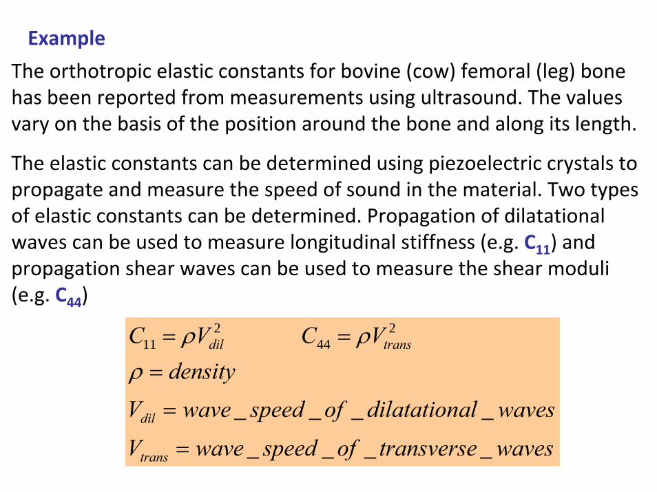
The orthotropic elastic constants for bovine (cow) femoral (leg) bone has been reported from measurements using ultrasound. The valuesvary on the basis of the position around the bone and along its length. 

The elastic constants can be determined using piezoelectric crystals to propagate and measure the speed of sound in the material. Two types of elastic constants can be determined. Propagation of dilatational waves can be used to measure longitudinal stiffness (e.g. C11) and propagation shear waves can be used to measure the shear moduli(e.g. C44) 

wavestransverseofspeedwaveV

wavesaldilatationofspeedwaveVdensity

VCVC

trans

dil

transdil

____

____

244

211

=

=

===

ρρρ

The approximately reported stiffness values are: 

MPa

⎥⎥⎥⎥⎥⎥⎥⎥

⎦

⎤

⎢⎢⎢⎢⎢⎢⎢⎢

⎣

⎡

3.50000003.600000070000002578.400074.183.60008.43.614

Find the Young Modulus along the bone length (z‐direction)? And along the radial direction (x and y directions).

Find the Poisson’s ratios? 

Convert the stiffness matrix into a compliance matrix.

1

19.000000016.000000014.0000000046.0014.0009.0000014.007.0026.0000009.0026.0086.0

−

⎥⎥⎥⎥⎥⎥⎥⎥

⎦

⎤

⎢⎢⎢⎢⎢⎢⎢⎢

⎣

⎡

−−−−−−

MPa

1044.00090 28.1407.011

3016.00260 6.11086.011

373.00260 7.21046.011

131

13

222

121

12

111

212

21

333

=⇒−====

=⇒−====

=⇒−====

υ

υ

υ

.Eυ-GPa

SE

.Eυ-GPa

SE

.Eυ-GPa

SE

ExampleDetermine the modulus of elasticity for iron single crystals in the <111>, <110> and <100> directions.

31

31

31111

02

12

1110

001100nmlDirections

nwvu

uvwCos

mwvu

uvwCos

lwvu

uvwCos

=++

=

=++

=

=++

=

222

222

222

1))(001(

1))(010(

1))(100(

γ

β

α

60.88.20.810 441211

13

−

−−

FeSSSGPa

( )

GPaEE

125

0.8)0(26.88.20.820.81

100

100

=

=⎟⎠⎞

⎜⎝⎛ −−−−=

( )

GPaEE

270

7.3)91

91

91(

26.88.20.820.81

111

111

=

=++⎟⎠⎞

⎜⎝⎛ −−−−=

( )

GPaEE

210

75.4)0041(

26.88.20.820.81

110

110

=

=++⎟⎠⎞

⎜⎝⎛ −−−−=