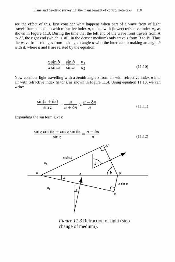
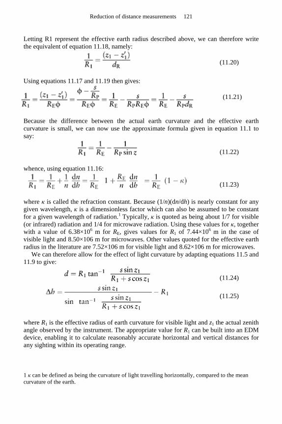
plane and geodetic surveying: the management of control networks
TRANSCRIPT

Plane and Geodetic Surveying
Plane and Geodetic Surveying blends theory and practice conventional techniques and GPS to provide the ideal book for students of surveying
Detailed guidance is given on how and when the principal surveying instruments (theodolites total stations levels and GPS) should be used Concepts and formulae needed to convert instrument readings into useful results are fully and clearly explained Rigorous explanations of the theoretical aspects of surveying are given while at the same time a wealth of useful advice about conducting a survey in practice is provided An accompanying least-squares adjustment program is available to download from wwwsponpresscomsupportmaterial
Developed from material used to teach surveying at Cambridge University this book is essential reading for all students of surveying and for practitioners who need a lsquostand-alonersquo text for further reading
Aylmer Johnson is a Senior Lecturer in the Cambridge University Engineering Department and a Fellow of Clare College His main research interests are in the area of computer-aided embodiment design but he has also taught surveying for 25 years and now leads the Surveying Group at Cambridge University
Plane and Geodetic Surveying The management of control networks
Aylmer Johnson
LONDON AND NEW YORK
First published 2004 by Spon Press 11 New Fetter Lane London EC4P 4EE
Simultaneously published in the USA and Canada by Spon Press 29 West 35th Street New York NY 10001
Spon Press is an imprint of the Taylor amp Francis Group This edition published in the Taylor amp Francis e-Library 2005
ldquoTo purchase your own copy of this or any of Taylor amp Francis or Routledgersquos collection of thousands of eBooks please go to httpwwwebookstoretandfcoukrdquo
copy 2004 Aylmer Johnson
All rights reserved No part of this book may be reprinted or reproduced or utilised in any form or by any electronic mechanical or other means now known or hereafter invented including
photocopying and recording or in any information storage or retrieval system without permission in writing from the publishers
British Library Cataloguing in Publication Data A catalogue record for this book is available from the British Library
Library of Congress Cataloging in Publication Data Johnson Aylmer 1951- Plane and geodetic surveying the management of control networksAylmer Johnson p cm Includes bibliographical references and index ISBN 0-415-32003-8 (hbk alk paper)mdashISBN 0-415-32004-6 (pbk alk
paper) 1 Surveying 1 Title TA545 J64 2004 5269ndashdc22 2003022666
ISBN 0-203-63046-7 Master e-book ISBN
ISBN 0-203-34532-0 (Adobe e-Reader Format) ISBN 0-415-32004-6 (Print Edition)
To Vanya my wife who has given me unstinting support while enduring many solitary evenings during the production of this book
Contents
Preface ix
Acknowledgements xi
1 Introduction 1
2 General principles of surveying 5
3 Principal surveying activities 12
4 Angle measurement 24
5 Distance measurement 39
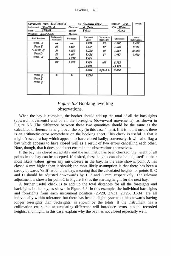
6 Levelling 44
7 Satellite surveying 53
8 Geoids and ellipsoids 68
9 Map projections 80
10 Adjustment of observations 97
11 Reduction of distance measurements 115
12 Reciprocal vertical angles 128
Appendices
A Constants ellipsoid and projection data 135
B Control stations 137
C Worked example in transforming between ellipsoids 140
D Calculation of local scale factors in transverse Mercator projections 142
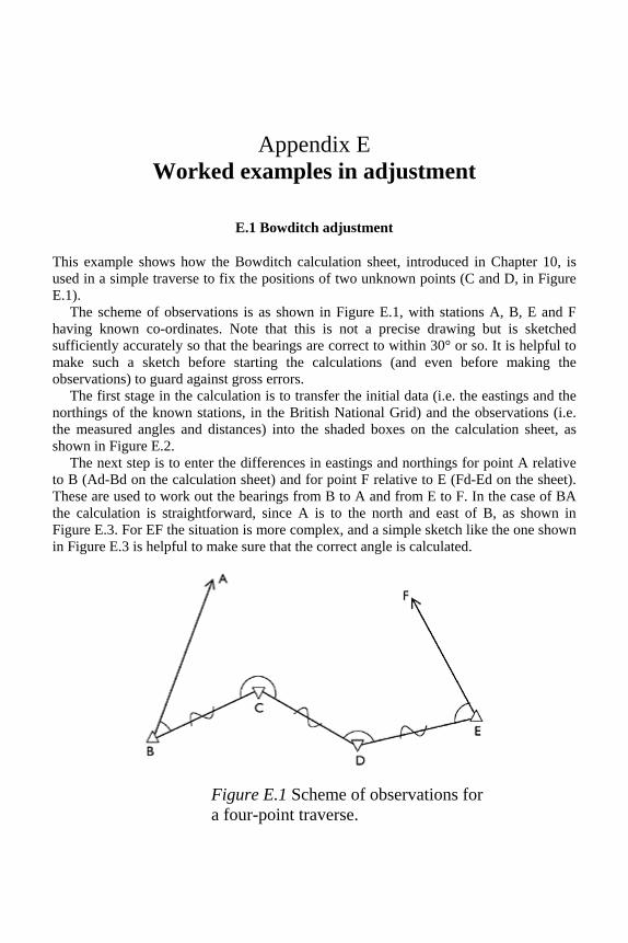
E Worked examples in adjustment 145
F Worked example in setting out 152
G Booking sheets 157
H Calculation sheets 162
Glossary 165
Bibliography 169
Index 171
Preface
More than almost any other engineering discipline surveying is a practical hands-on skill It is impossible to become an expert surveyor or even a competent one without using real surveying instruments and processing real data On the other hand it is undoubtedly possible to become a very useful surveyor without ever reading anything more theoretical than the instrument manufacturersrsquo operating instructions
What then is the purpose of this book A second characteristic of surveying is that it involves much higher orders of accuracy
than most other engineering disciplines Points must often be set out to an accuracy of 5 mm with respect to other points which may be more than 1 km away Achieving this level of accuracy requires not only high-quality instruments but also a meticulous approach to gathering and processing the necessary data Errors and mistakes which are minute by normal engineering standards can lead to results which are catastrophic in the context of surveying
Yet in the real world errors will always exist and approximations and assumptions must always be made The accepted techniques of surveying have been developed to eliminate those errors which are avoidable and to minimise the effects of those which are not Likewise the formulae used by surveyors incorporate many assumptions and approximations and save time when the errors which they introduce are negligible by comparison with the errors already inherent in the observations
No two jobs in surveying are exactly the same A competent professional surveyor therefore needs to know the scope and limitations of each surveying instrument technique and formulamdashpartly to avoid using unnecessarily elaborate methods for a simple job but mainly to avoid using simplifying assumptions which are invalidated by the scale or required precision of the project This knowledge can only be developed by understanding how the accepted techniques have evolved and how the formulae workmdashand this understanding is becoming increasingly hard to acquire with the advent of electronic lsquoblack boxrsquo surveying instruments and software applications which perform elaborate calculations whose details are hidden from the user
It is this understanding which this book sets out to provide The methods for using each generic class of surveying instrument have been described in a way which is intended to show why they have evolved and the calculations are similarly explained such that the inherent assumptions can be clearly identified Wherever necessary practical guidance is also given on the range of distances for which a particular formula or technique is both necessary and valid
The material in this book is based on the surveying courses taught in the Engineering Department at Cambridge University and I am grateful to the many colleagues who have both enhanced my own understanding of the subject and contributed to past editions of the lsquoSurvey Notesrsquo from which this book has evolved The philosophy of engineering education at Cambridge has always been that an understanding of a subjectrsquos fundamental principles is the key to keeping abreast with the changes which technology inevitably
brings and indeed to initiating appropriate changes when technology makes this possible I hope that this book has succeeded in applying that philosophy to surveying in a way which will be of value to those who read it
Aylmer Johnson Cambridge
August 2003
Acknowledgements
I am indebted to the many colleagues and students who have helped to shape the various drafts of this text and the accompanying computer program In particular I would like to thank John Matthewman who taught me much of what I know about surveying and Jamie Standing who encouraged me to write this book The late Wylie Gregory also deserves special mention as the original author of the core algorithms within the adjustment program
Chapter 1 Introduction
11 Aim and scope
Engineering works such as buildings bridges roads pipelines and tunnels require very precise dimensional control during their construction Buildings must be vertical long tunnels must end at the correct place and foundations must often be constructed in advance to accommodate prefabricated structural sections To achieve this surveyors are required to determine the relative positions of fixed points to high accuracy and also to establish physical markers at (or very close to) predetermined locations These tasks are achieved using networks of so-called control points this book aims to give the civil engineering surveyor all the necessary theoretical knowledge to set up manage and use such networks for the construction and monitoring of large or small engineering works
The exact way in which control networks are established and managed depends on a number of factors
1 The size of the construction project and the accuracy required The accuracy of each technique described in this book is explained together with the limitations of the various assumptions used in subsequent calculations In particular guidance is given as to when a project is sufficiently large that the curvature of the earth must be taken into account
2 The available equipment As far as possible the descriptions of surveying equipment in this book are generic and are not based on the products of any one particular manufacturer Both GPS and lsquoconventionalrsquo surveying equipment are covered since both are appropriate under different circumstances
3 The country in which the work is being carried out This book explores some topics with particular reference to the mapping system used in Great Britain but a clear indication is also given of how the same issues are addressed in other countries with different mapping systems and survey authorities
The tools of the engineering surveyor have changed significantly in recent years Most notably GPS is now the simplest and most accurate way of finding the position of any point on the surface of the earth or (more importantly) the relative positions of two or more points However GPS has some inherent limitations which are explained in detail in Chapter 7 As a result other more conventional surveying techniques must still be understood and used when appropriate In addition the traditional surveying tools such as levels and theodolites are now predominantly electronic and can usually record (and even observe) readings quite automatically The descriptions in this book are largely independent of these advances because they do not change the basic way in which the instrument works but simply mean that readings can be taken more simply and quickly
The particular techniques for using manual instruments have also been included for those occasions and locations where electronic instruments are not available or appropriate
12 Classification of surveys
Surveys are conducted for many different purposes which will determine the type of instruments which are used the measurements which are taken and the subsequent processing of those measurements to produce the required results It is useful to know the names of the principal types of survey and the nature of the work which is involved
Engineering surveys are usually classified in the following ways
By their purpose
1 Geodetic To determine the shape of the earth or to provide an accurate framework for a big survey whose size means that the curvature of the earth must be taken into account
2 Topographic To produce ordinary medium-scale maps for publication and general use Topographic surveys record all the features of the landscape which can be shown on the scale of the map Topographic maps are usually produced by means of aerial or satellite photogrammetry
3 Cadastral To establish and record the boundaries of property or territory Concerned only with those features of the landscape which are relevant to such boundaries
4 Engineering To choose locations for and then set out markers for engineering construction works Engineering surveys are concerned only with the features relevant to the task in hand
Engineering surveyors are likely to come in contact with all these types of survey but are less likely to have to conduct a topographic survey For this reason the techniques of topographic surveying are not covered in this bookmdashfor further information on this class of surveying see Mikhail et al (2001) and Wolf (2000)
By their scale
The scale of a survey will affect the instruments and techniques used as well as the type of projection used to display or record the results In a topographic survey it will also determine the amount and type of topographic detail which is recorded
By the type of measurements taken
1 Triangulation Finding the size and shape of a network of triangles by measuring sides and angles Used when each station can see three or more other stations
2 Traverse Proceeding from one point to another by lsquodead reckoningrsquo using measured distances and angles to calculate bearings Used when the construction work is long and narrow such as a motorway or tunnel
Plane and geodetic surveying the management of control networks 2
3 Resectioning Establishing the position of a single station by measuring distances and angles to a number of other nearby stations whose positions are already known
4 DGPS Measuring the relative 3D positions of two stations by simultaneously recording GPS data at each one and comparing the results
Often a particular survey involves a hybrid of all four of these techniques
By the equipment used
1 Tape For direct linear measurement Cheap and robust Still occasionally used for small detailed surveys but now largely supplanted by laser-based distance measurement devices
2 Compass To observe bearings Used mainly in reconnaissance 3 Theodolite A telescopic sight pivoted horizontally and vertically with two graduated
protractors (called lsquocirclesrsquo) for measuring angles See Figure 11 4 Electromagnetic distance measurement (EDM)devices Typically used for
measurements of lengths from say 5 m to 5 km though some instruments have ranges up to about 25 km
5 Total station Essentially a theodolite with a built-in EDM Total stations usually have facilities for recording and processing measurements electronically and have largely replaced conventional theodolites
Figure 11 Angles measured by a theodolite
Introduction 3
6 GPS Position fixing by satellite has almost completely replaced terrestrial triangulation for large-scale control survey and can also be useful on building sites provided it is not set up close to buildings or trees
7 Aerial camera photogrammetry) Mainly used in topographic surveys but also for recording the shapes (and subsequent deformations) of buildings See Atkinson (2001)
8 Satellite camera Essentially a long-range aerial camera
13 The structure of this book
There is no single logical order in which to set out the further theoretical knowledge that a competent engineering surveyor will need The approach adopted in this book has been to outline the most important principles of surveying in Chapter 2 and the main activities of surveyors in Chapter 3 This is followed by four further chapters explaining how particular measurements are made angles in Chapter 4 distances in Chapter 5 heights in Chapter 6 and satellite position fixing in Chapter 7 The use of satellite data in particular requires an understanding of geodesy including the shape of the earth and the co-ordinate systems used to describe the positions of points on or near to its surface these concepts are explained in Chapters 8 and 9 Chapters 10 and 11 discuss the main calculations a surveyor will need to process raw observations into useful results Chapter 12 describes a specialist method for finding height differences which is particularly useful for tall structures and for establishing local transforms for GPS data
The appendices contain useful numerical data observation and calculation sheets and worked examples of some of the calculations described in the book A Glossary is also included explaining words which might be unfamiliar to the reader
Finally a least-squares adjustment program called LSQ is included as part of this book LSQ will adjust a mixture of DGPS and conventional observations to compute the most likely positions of stations whose positions are unknown and the likely accuracy to which they have been found
Plane and geodetic surveying the management of control networks 4
Chapter 2 General principles of surveying
Surveying has two notable characteristics the work is done to a much higher level of accuracy than most other engineering work and it is easy for quite serious errors to remain undetected until it is too late to correct them For this reason there are some inherent principles which should be observed in all surveying regardless of the type of survey or the equipment used This chapter describes those principles
21 Errors
All the results of surveying are based on measurements and all measurements are subject to errors Because surveying involves high degrees of accuracy (most surveying measurements are accurate to within 10 parts per million and some are within 2 parts per million) it is relatively easy to make errors and relatively hard to detect them The understanding and management of errors is therefore possibly the single most important skill that a professional surveyor must possess Many of the techniques of surveying are directed towards cancelling or eliminating errors and towards ensuring that no serious error remains undetected in the final result Even so the presence of unnoticed lsquosystematicrsquo errors in a survey can lead to false yet seemingly consistent results A recent international tunnelling project drifted several metres from its intended path because temperature gradients near the tunnel wall caused laser beams to bend and this was not detected until an independent method was used to check the work
High accuracy in surveying is expensive because it involves costly high-quality equipment and more elaborate procedures for taking measurements On the other hand cheaper equipment may not be adequate to achieve the required accuracy particularly if (for instance) a long distance has to split into several steps requiring more measurements and resulting in an accumulation of errors Surveys are therefore often conducted by using high-quality equipment to establish a few lsquomajor controlrsquo stations around the area to a higher precision than is required overall and then filling in the intervening detail by cheaper methods adequate for the shorter distances This is usually the most economic way of distributing the lsquoerror budgetrsquo to achieve a satisfactory final result at minimum cost
Types of errors
Surveying errors fall into three categories
1 Blunders (or gross errors) Blunders are due to mistakes or carelessness such as misreading by a metre or a degree A proper routine of checks should detect them A
surprisingly common source of error is the manual transcription of readings from one place to another
2 Systematic errors Systematic errors are cumulative and due to some persistent causemdashgenerally in an instrument but sometimes in a habit of the observer They can be reduced by better technique but not by averaging many readings as they are not governed by the laws of probability Thus all distances measured with an inaccurate tape or EDM will from that cause have the same percentage or absolute error whatever their lengths and however many times they are measured the only remedy is to calibrate the device more carefully This is the most serious sort of error and the technique of survey is mainly directed against itmdashthe greater the accuracy required the more elaborate and expensive the instruments and the technique
A special type of systematic error is a periodic error which varies cyclically within the instrument Examples include errors in the positions of the angle markers on a horizontal circle or non-linearities in the phase resolver of an EDM or GPS receiver This type of error can sometimes be eliminated by special observation techniques eg measuring a horizontal angle several times but using a different part of the horizontal circle on each occasion
3 Random errors Random errors are due to a number of small causes beyond the control of the observer Their magnitude depends on the quality of the instrument used and on the skill of the observer but they cannot be corrected Thus no one can place a mark or make an intersection or read a scale with absolute accuracy or consistency Even after allowing for systematic personal bias (covered in 2 above) there will remain errors which are a matter of chance and are subject to the laws of probability In general positive and negative errors are equally probable small errors are more frequent than large ones and very large random errors do not occur at all
In statistical terms random errors cause readings to deviate from the correct value in the manner of a normal distributionmdashsimilar for instance to the scatter of heights to be found in a sample of adults The scale of the scattering can therefore be defined by quoting the standard deviation (σ) of the distribution two-third of all readings will lie within one standard deviation of the correct value (above or below) and 95 per cent within two standard deviations Alternatively the standard deviation for a reading can be estimated by taking the measurement several times and seeing what range of values covers the middle two-third of the readings the size of this range is an estimate of 2timesσ Two other measures of quality are also used to define the accuracy of readings affected by random errors The probable error expressed as plusmnp is such that 50 per cent of a large number of readings differ from the correct value by less than p for normally distributed errors p is 0675 times the standard deviation of the readings A more useful measure of accuracy is the 95 per cent confidence value which as explained above is almost exactly two standard deviations Assuming that the observation errors from an instrument have a normal distribution (ie that they contain no gross or systematic errors) it can be shown that the standard deviation associated with the arithmetic mean of a set of n repeated observations is times the standard deviation of a single observation Thus if a single angle measurement can be read to one second of arc the mean of four readings should have a precision of 05 seconds Taking the
Plane and geodetic surveying the management of control networks 6
same measurement several times can therefore be a valid way of increasing the overall accuracy of a survey
It is however important to understand the distinction between precision and accuracy It is possible to read an angle to considerable precision as described abovemdashbut if the circle (ie optical or electronic protractor) in the instrument is poorly made the reading will still be inaccurate Even when the greatest precautions are taken in making a reading (eg measuring the angle again using a different part of the circle) systematic errors may still dominate the results Too much importance must not therefore be attached to the estimated standard deviations (ESDs) of a set of observations based on the apparent lsquoscatterrsquo of the results A set of consistent readings indicates a consistent instrument and a good observer but not necessarily an accurate result
22 Redundancy
Given two points whose positions are known the position of a third point in plan view can be found by (for instance) measuring the horizontal distances between it and the two known points However the accuracy of the calculated position can only be inferred from the quoted accuracy of the distance measurement device and a gross error in one of the distance measurements (or an error in the quoted position of one of the known points) will still give a seemingly plausible solution for the new pointrsquos position
To overcome both of these problems a fundamental principle of surveying is to take redundant readings ie to take more measurements than are strictly necessary to fix the unknown quantities Any large inconsistency in the readings will then indicate a gross error in the measurements or the data while any small inconsistencies will give an unbiased indication of the likely accuracy to which the point has been fixed
When several new points are to be fixed simultaneously it can become quite difficult to ensure by simple inspection that enough suitable readings have been taken or planned to ensure redundancy throughout the network This soon becomes apparent though when the readings are adjusted (see Section 24) by computer For this reason many adjustment programs include a planning mode which enables a proposed scheme of observations to be validated for redundancy before it is carried out A surveyor is strongly advised to carry out such a check if there is any doubt about the redundancy of a proposed scheme of observations
23 Stiffness
In addition to being redundant a network (and its associated observations) should also be lsquostiffrsquomdashin other words the relative positions of control points and the scheme of observations should be arranged such that any significant movement of one of the points would cause a correspondingly significant change in at least one of the observations This ensures that the positions of unknown points are established to the highest possible accuracy using the instruments which are available
There is an exact analogy (as with redundancy) between a lsquostiffrsquo network and a lsquostiffrsquo structure The pin-jointed structure shown in Figure 21 (a) is stiff because any given
General principles of surveying 7
deflection of point C requires that member AC or BC (or both) must lengthen or shorten by a similar amount In Figure 21(b) by contrast the structure is much less stiff since C can make quite large vertical movements with relatively small changes in the lengths of the two members
Figure 21 Stiff and non-stiff structural frameworks
Figure 22 Stiff and non-stiff survey networks
The corresponding situation in surveying is shown in Figure 22 where points A and B are lsquoknownrsquo points and C is unknown and the distances AC and BC have been measured As with the structure Figure 22(a) shows a stiff network in which any significant movement of point C would involve equally significant changes to one or both of the measured distances whereas in Figure 22(b) C could move significantly in the northsouth direction without greatly affecting either of the distances
If angle measurements are used as well this corresponds to adding gusset plates to the structure which increases its stiffness by removing the freedom in the pin joints
As with redundancy it can be quite difficult to determine by inspection whether a proposed scheme of observations will result in a stiff network Again though an adjustment program with a lsquoplanningrsquo facility will provide a good prediction of how
Plane and geodetic surveying the management of control networks 8
accurately the unknown points will be fixed if the likely accuracy of the planned observations is known
24 Adjustment
As explained in Section 22 the position of new points should always be found by taking more observations than are strictly necessary Inevitably then the resulting readings will be in conflict because of the small random errors in the readings there will be no single set of positions for the new points which will be in exact agreement with all the measurements
To resolve this problem some form of lsquoadjustmentrsquo is usually applied to the calculated position of the point to give the best fit with the measurement data The commonest method is called least-squares adjustment which chooses positions for the new points such that the sum of the squares of the residual errors1 is minimised This gives the most likely positions for the new points assuming that the observation errors are normally distributed
A good understanding of what adjustment can and cannot achieve is important for a surveyor Essentially it is a statistical process which gives the most likely position for each new point assuming that the observation errors are random and normally distributed If this is not the case the results may be misleading or inaccurate In particular least-squares adjustment will give a false impression of accuracy if there are systematic errors present in the data eg if all distance measurements are made using a device which is poorly calibrated It will also generate misleading results if the user is tempted to reject any seemingly lsquobadrsquo observations purely on the grounds that they do not appear to agree well with the others
Adjustment is described in greater detail in Chapter 10
25 Planning and record keeping
A successful survey requires an appropriate set of measurements to be taken and recorded without unnecessary deployment of human resources or equipment This can only be achieved by means of planning The following guidelines will improve the quality of any surveying work
1 Establish clearly what the purpose of the survey is and what additional uses it might be put to in the future This will determine the number and the locations of control points and the accuracy to which their positions must be found
1 The residual error is defined as the difference between an observed angle or distance and the calculated value based on the assumed position(s) of the new point(s)
General principles of surveying 9
2 Find a suitable map or satellite photograph of the site to be surveyed This will help in the creation of a possible network of control points in suitable locations and with adequate stiffness It will also show the approximate scale of the work and will help in detecting gross errors in angle and distance measurements
3 Visit the site if at all possible Check whether control stations can be sited at the places indicated by step 2 and make a note of what will be needed to build them If conventional instruments are to be used check whether the necessary lines of sight exist between the station locations using ranging rods if necessary If GPS is to be used check that the relevant stations have a clear view of the sky Make notes of any features on the site (cliffs ditches etc) which might make it difficult to move from one station to another
A few simple instruments may also help at this stage A compass can be used to estimate horizontal angles and a clinometer will measure approximate vertical angles A hand-held GPS receiver will give the approximate co-ordinates of points and estimates of the distances between them If this is not possible the distances can be paced
4 Plan a set of observations which will establish the control network to the required accuracy at minimum cost This is generally best done by working lsquofrom the whole to the partrsquo accumulated errors are minimised by first forming an accurate framework covering the whole area and then adding further control stations to whatever accuracy is necessary Accurate measurements require expensive equipment and longer observation times so this type of consistent approach will give the most economical result
The planning function in an adjustment program is very useful here The eventual quality of a network can be reliably predicted by entering approximate observations (such as the compass angles above) together with estimates of the accuracy to which the final measurement will be made2 Different observations can then be included in the scheme to see which combination will give an adequate accuracy for minimum investment Make sure though that there are enough observations so that one or more could be rejected without unacceptable loss of accuracy or redundancy The time spent travelling to and from a site is usually much greater than that needed to take a few lsquosparersquo measurements while an instrument is set up
5 Plan the fieldwork in detail to make sure that all the necessary measurements are taken with the minimum deployment of people and equipment Each member of the team should know who will take which measurements at which locations and with what instruments
6 If possible arrange that all field work has redundancy and that the computations are carried out such that no incorrect measurement will pass undetected If some of the error checks can be carried out in the field while the equipment is still set up on station then the cost of correcting any error will be greatly reduced
2 The approximate observations establish the geometry of a network to sufficient accuracy for its eventual stiffness to be determined This combined with the accuracy of the final observations determines the accuracy to which the points in the network will eventually be fixed
Plane and geodetic surveying the management of control networks 10
7 Before leaving base make sure that all batteries are fully charged and that any necessary co-ordinate data transformations etc have been downloaded into those instruments that need it Make sure that everyone is familiar with the instruments they will be using get unfamiliar instruments out read the instruction manuals and practise their use
8 Ensure that each group of surveyors keeps a diary of what is done including a summary of the weather on each day If an error is discovered later a good diary can be invaluable in pinpointing the source of the problemmdashand thus showing which measurements may need to be repeated
9 Make sure that observation records are complete and will not degrade with time Handwritten records must be legible and electronic records should be stored securely eg on a CD If the information is important make sure that there are two copies of it in different locations the cost of this is minuscule compared to the cost of taking the measurements again
The data generated during a surveying job may need to be consulted years after it was initially made so good record keeping is also important Observations recorded on paper should be checked for legibility and completeness and stored in a dry condition electronic data should be stored on a permanent medium such as a CD-ROM For important jobs copies of the data should be made and stored in a different location to the originals Finally a brief summary of the data will greatly assist any subsequent attempt to re-inspect some part of it
General principles of surveying 11
Chapter 3 Principal surveying activities
31 Managing control networks
Before any survey can yield useful results it is necessary to establish a set of fixed stations whose positions relative to one another are knownmdashusually to a higher accuracy than will be needed in the final result A set of such stations is known as a control network
If the scope of an engineering project is relatively small (up to 5 km square say) and does not have to be tied in with work elsewhere then it is usually easiest to set up a local Cartesian co-ordinate system for the work and to use conventional surveying instruments rather than GPS Typically the first control station1 is established at or near the south-west corner of the site and defined to be the lsquosite originrsquo having the co-ordinates (000)2 A second station is then set up at the north-west corner of the site with its x co-ordinate defined to be 0 The horizontal line between the two stations defines the y-axis or lsquosite northrsquo and the z-axis is defined to be vertically upwards An orthogonal Cartesian co-ordinate system is thus fully specified such that any point on the site has a unique (x y z or easting northing height) co-ordinate
Further control stations will also be needed on the site and each one is set up by first choosing a suitable location then physically establishing the station and finally taking measurements to find its co-ordinates The 2D (x y) position of each station is found by measuring horizontal angles andor distances to or from other stations (see Chapters 4 and 5) If needed the height (z) co-ordinates are usually found separately by levelling as explained in Chapter 6
If just one further control station was to be added to the initial two points there would be three unknowns in the 2D co-ordinate system namely the (x y) co-ordinates of the third control station and the y co-ordinate of station 2 Finding these unknowns with redundancy thus requires at least four measurements of which at least two must be horizontal distance measurements (if one distance and three angles were measured there would be no check that the distance had been measured correctly) A typical scheme of measurements for fixing a third station is shown in Figure 31 here a horizontal angle has been measured at station 1 and the instrument has then been moved to station 3 where a second angle and two distances have been measured
1 See Appendix B for a full discussion of control stations 2 Often a set of positive co-ordinates is chosen for the site origin eg (100 100 100) so that no point on the site has negative co-ordinates
If the final network is to consist of more than three control stations then a minimum of 2nminus2 readings is required to achieve redundancy in two dimensions where n is the total number of stations (ie including the origin and site north) In addition redundancy considerations require that
1 there should again be at least two distance measurements 2 site north (which has one unknown) should be involved in at least two measurements
and 3 each subsequent point (which will have two unknowns) should be involved in at least
three measurements
These requirements at least ensure that no gross error will pass unnoticedmdashbut it is generally advisable to take several additional measurements over and above this minimum so that any problematic reading can be eliminated from the set altogether without loss of redundancy
The total number of control stations required in the network and their relative positions will depend on the size of the site and the purposes for which they are needed If the intention is to set out further points on the ground whose own relative positions must be guaranteed to be accurate (eg the foundation points for a prefabricated bridge) then there should ideally be three or more control stations near to each point arranged so that the positions of the new points will be sufficiently accurate and totally error-poof when they are set out If the purpose includes the production of some type of map then each relevant feature of the landscape must be visible from (and not too far from) one of the control stations Further control stations may also be needed simply to ensure that the relative positions of the lsquousefulrsquo stations are known to a sufficient degree of confidence and accuracymdashand also to ensure that the site co-ordinate system will not be lost if one or both of the original stations were destroyed or displaced
Figure 31 Survey network with three control stations
Principal surveying activities 13
Many variants exist for establishing a local Cartesian system as described above There is no need for lsquosite northrsquo to be the same as true north though it reduces the likelihood of mistakes if they are more or less in the same direction Likewise the station which defines the lsquosite originrsquo does not have to be at the south-east corner of the sitemdashbut if it is not then the chances of gross errors are again reduced if its co-ordinates are not (000) but are defined such that every point on or around the site has positive co-ordinates
In larger surveys it is often necessary or more convenient to use an existing regional co-ordinate system or grid This is typically done by using nearby existing control stations with known co-ordinates to find the grid co-ordinates of the main control stations around the site Such grid systems are usually orthogonal but they often involve a scale factor this means that one metre in the grid system does not exactly correspond to one metre of horizontal distance on the ground On a very large survey this scale factor will alter between one place and another and this causes discrepancies between angles observed in the field and those measured between the corresponding straight lines drawn on the grid projectionmdashsee Chapter 9 for further details There are also complications in using a national datum for height measurements which are explained in Chapter 8
Since about 1980 the most straightforward way to find the relative positions of stations has been to use differential GPS GPS receivers are simultaneously placed on two different stations and their relative positions are known to within about 5 mm after approximately half an hourrsquos lsquoobservationrsquo If national grid co-ordinates are required one or more national GPS control points (whose grid co-ordinates are now typically published over the Internet) are also included in the scheme of observations A particular advantage of using differential GPS is that the stations do not need to have a line of sight between them The use of GPS is explained in Chapter 7
GPS has not however completely supplanted the more traditional ways of establishing control networks It cannot be used if the control stations need to be near tall buildings beneath trees or in tunnelsmdashand the computation required to transform the data into a ground-based co-ordinate system can only be checked by making conventional measurements between some of the control points as well The equipment is also relatively expensive and is potentially subject to undetectable systematic errors if used on its own so again it is reassuring to have an independent method of checking the results it produces The remainder of this section therefore describes the more traditional ways of establishing control networks
Triangulation
Until about 1970 all control networks were set up by a process called triangulation Two stations were established on the ground and the distance between them (called the lsquobase linersquo) was carefully measured3 The relative position of a third station could then be fixed (with partial redundancy) by measuring all three angles in the triangle between it and the other two stations no further distance needed to be measured which was an advantage in
3 Accuracy is crucial here since any error in this measurement will cause an undetectable lsquoscale errorrsquo to propagate through the whole network
Plane and geodetic surveying the management of control networks 14
the days when distances could only be measured by tape More stations could subsequently be added to the network by measuring angles between them and two or more of the stations already in the net
For a given instrument accuracy and time budget the best overall control network for a particular area using triangulation is obtained by distributing control stations as evenly over the area as possible with well-conditioned4 triangles and most stations visible5 from at least three others Since each extra station requires at least three extra observations to fix its horizontal position the total number of stations is kept as low as possible at this stage if further control is subsequently required in part of the area more stations can be established nearby and fixed with reference to the existing stations6
The advent of electromagnetic distance measurement (EDM) in about 1970 made distance measurement much easier and cheaper and meant that many of the sides of the triangles in such networks could now be measured as well This has the effect of making any network much lsquostifferrsquo and eliminates the possibility of an undetected scale error However the use of distances to fix the grid positions of stations even in two dimensions requires knowledge of the altitudes of the endpoints as will be shown in Chapter 11mdashso the use of distance measurements is sometimes kept to a minimum in conventional surveys even now
Traversing
When the area to be controlled is long and thin (eg a new motorway) or when each station can only see two others a system of interlocking triangles is impracticable and a so-called traverse is used instead In its simplest form this consists of setting up a total station over a station whose co-ordinates are known observing another lsquoknownrsquo station then observing the angle and distance to a station whose position is unknown but which can now be calculated from the information available The instrument is now set up over the new station and the process is repeated for each lsquounknownrsquo station in turn finishing up on a final lsquoknownrsquo station The agreement between the calculated co-ordinates and the known co-ordinates for this final station is a measure of the accuracy of the traverse and there are two pieces of redundancy in the set of observations which can be used to give improved estimates of the positions of all the unknown stations in the traverse
In practice most control networks are now established by some hybrid of triangulation traverse and GPS The key features of a good network are that it should be both stiff and redundant as described in Chapter 2 and that if possible it should be free of any possibility of systematic error 4 No angle in the triangle should be less than about 20deg or greater than about 160deg 5 Two stations cannot be regarded as being visible from each other if the line of sight between them passes close to (lsquograzesrsquo) some piece of intervening ground This will have the effect of bending the light path between them greatly reducing the accuracy of angle and distance measurements 6 This was the logic which dictated the construction of the first-order network over the United Kingdom by the Ordnance Survey between 1936 and 1951 There are approximately 480 first-order stations covering Great Britain most of which are at the tops of hills or mountains in flat parts of the country Church towers and water towers are used instead A much larger network of second-order stations was subsequently established using the first-order stations as fixed points
Principal surveying activities 15
32 Mapping
This book does not attempt to cover mapping to the depth required by cartographers however engineering surveyors will sometimes need to make maps of small areas so a few useful guidelines are given here
1 Decide what scale of map is required before starting On a 11000 map a line of width 02 mm will represent 02 m on the ground so there is no value in recording the positions of points to better than this accuracy
2 For the same reason there is no value in recording details of shape which are too small to show up on the map If a length of fence or hedge does not deviate from a straight line by more than one linersquos width when plotted on the map then only the positions of the endpoints need be recorded
3 The purpose(s) of the map will determine what details need to be recorded and how this should be done If the map is to be used to plan the positions of new control points then the line which records say the edge of a ditch should mark the closest point to the ditch where it would be sensible to establish a control point rather than the waterrsquos edge Likewise the diameter of a treersquos trunk might be of relevance for determining lines of sight on the ground while the size of its canopy will be of relevance for GPS
4 It is useful to draw a freehand sketch of the intended map before starting to take measurements This will help show the amount of detail which can usefully be recorded and can be marked up with numbers which relate to the points whose positions are actually measured
5 If points are to be recorded by means of a total station it will first be necessary to establish control points such that every point of interest can be observed from one control point or another Also each control point used for mapping must have a line of sight to some other known point which can be used as a reference bearing for the other measurements If the control points are only needed for mapping purposes then their positions probably do not need to be known to better than decimetre accuracymdashbut it may be wise to establish them to higher accuracy than this in case they are subsequently used for some other purpose
6 To make a map the instrument is first sighted on a reference object Some instruments can then use the co-ordinates of the instrument position and reference object to lsquoorientrsquo themselves and calculate co-ordinates for all subsequent sightings A staff-holder then takes a detail pole (with a reflector) to each point of interest and the bearing and the distance are recorded by the instrument Some total stations are motorised and follow the target automatically the surveyor with the detail pole can then tell the instrument when to take the readings by means of a radio link This means that the job of collecting detail can be done by a single surveyormdashbut there have been cases of motorised total stations being stolen when the surveyor is too far away to prevent it
7 Small areas are now often mapped using real time kinematic GPS The operator walks from one point of interest to another and records their positions using a GPS receiver in a small backpack An electronic map can be produced simultaneously by joining the points with curves or straight lines and adding symbols or descriptive text using a hand-held computer
Plane and geodetic surveying the management of control networks 16
As well as making land maps surveyors sometimes need to lsquomaprsquo complex shapes such as the faccedilade of a building or the steelwork of a bridge Devices are now available to do this relatively automatically essentially these are high-speed motorised reflectorless total stations which systematically scan across their field of view and produce a 3D lsquopoint cloudrsquo of observations These can be fed into solid modelling software which will lsquoclothersquo the points with a surface to produce a computer model of the object If several point clouds are captured from different viewpoints and combined a complete solid model can be produced
33 Setting out
The most common ultimate purpose of an engineering survey is to lsquoset outrsquo points at predetermined positions on the ground or on partly built structures to mark where foundation points should be built for a new constructionmdashsuch as a roadway or a prefabricated bridge or the next storey of a building
The full range of setting-out procedures for different engineering purposes is not covered in this book but is very well and fully described both in Schofield (2001) and in Uren and Price (1994) Instead this section describes how to set out single points to the highest possible accuracy and Section 35 describes how to assess that accuracy once the location has been determined
Setting out in the horizontal plane
If the point is in a suitable place for GPS observations7 and the transformation between the GPS and the local co-ordinate system has been established then real time kinematic GPS can be used to lsquosteerrsquo the operator to the desired point usually to an accuracy of a centimetre or two Prolonged observation at that provisional point will then determine its position to a higher accuracy and an appropriate small movement can be made to improve the location of the point
If GPS is not available or appropriate new points can most easily be set out in the horizontal plane by calculating their bearings and distances from an existing control station whose co-ordinates are known A total station is set up on the existing station and sighted onto another control station to provide a reference bearing The angle to be turned through and the distance to be measured8 are calculated by simple geometrymdashsee Appendix F for a worked example of these calculations The instrument is turned through the appropriate angle and a target is moved until it is on the total stationrsquos line of sight and at the appropriate distance which places it at (or close to) the desired point Many total stations can perform these calculations automatically given the co-ordinates of the two control stations and the new point and will make an audible noise when the target is in the correct place
7 See Chapter 7 for an explanation of why some places are unsuitable for GPS 8 Remember that distances may need to be corrected for the local scale factor of the grid and for the heights of the two stationsmdashsee Chapters 9 and 11
Principal surveying activities 17
As with control networks it is essential to have some degree of redundancy when setting out new points so that any error will be detected before construction work starts The simplest form of redundancy is to set the point out again using different control points as reference points if the two resulting points are reasonably close to each other the point halfway between them can be used as the lsquobest guessrsquo for the point to be set out
An alternative method which avoids the use of distances involves setting up theodolites over three nearby control points (not necessarily simultaneously) and sighting them along the relevant bearing lines towards the new point as described above A small lsquosetting-out tablersquo is fixed in approximately the correct position and the lines of sight from the three theodolites are plotted on its surface to give a figure similar to that shown in Figure 32
Generally the lines will not cross at a point due to errors in the positions of the three control points and in setting up the three lines of sight However they should very nearly do somdashthe sides of the triangle should not be greater than a centimetre or two Assuming that the error is likely to be distributed equally between all three lines the most likely position of the required point is at the centre of the inscribed circle as shown in the figure-and the radius of the circle gives an indication of the likely accuracy to which the position of the point has been established
The following points are relevant to this method of setting out
1 Three lines of sight from existing control stations are necessary to guard against the possibility of a gross error eg in calculating one of the bearings Two lines will always cross at a pointmdashif the third one also passes nearby it is reasonably unlikely that any gross error has occurred
Figure 32 Establishing the best position for a set-out point
2 The three control stations should be positioned such that the triangle formed by the lines of sight is a reasonably well-conditioned one as shown in Figure 32 If two lines of sight cross each other at a very acute angle (less than about 30deg) then the accuracy
Plane and geodetic surveying the management of control networks 18
of the final point will be degraded as it would be strongly affected by a small movement of either of the two lines Note however that this does not require the control stations to be spaced at near minus120deg intervals round the set-out point as each station can be at either end of the line of sight
3 The reference object should be as far away from the control point as possible and at least as far away as the point to be set out Otherwise any inaccuracies in the relative positions of the reference object and the control point will cause a larger inaccuracy in the setting out
4 The lines of sight are drawn on the table by first holding a small marker (perhaps a pencil) on the edge of the table nearest to the theodolite and allowing the observer to lsquosteerrsquo it onto the line of sight This operation is repeated on the far edge of the table and the two points are joined by a straight line
5 For greatest accuracy each lsquoline of sightrsquo will actually consist of two linesmdashone from using the theodolite in its lsquocircle leftrsquo configuration and one from lsquocircle rightrsquo (see Section 44) The two lines should lie close to one another if the instrument is well adjusted and they should also be parallel if the marker has been lsquosteeredrsquo carefully by the observer A final line is then drawn halfway between the two observed lines and is taken as the lsquoline of sightrsquo from that theodolite
6 It is not necessary to have three theodolites for this task The table can be positioned and the first two lines drawn using two theodolites set up on two of the control stations When this has been done one of them is moved to the third control station and the final line is drawn on the table If only one theodolite is available the first lsquoline of sightrsquo can be approximately recorded using two ranging rods with a piece of string tied between them The theodolite is then moved to the second control station and the table is positioned where the second line of sight crosses the taut string Lines are now drawn on the table from the second station and the theodolite is then moved to the first and third stations for the other lines
7 If three well-conditioned lines cannot be sighted onto the table then two lines are drawn and a suitable target is set up above the intersection The horizontal distance to the intersection is then measured from one control station and compared with the calculated distance A third straight line can then be drawn on the table perpendicular to the corresponding line of sight and the appropriate distance from the intersection to give a locus of all points on the table which are the lsquocorrectrsquo distance from that control station An inscribed circle can then be drawn to touch the three lines as above
8 When the most likely position of the point has been established on the setting-out table a tripod can be set up over it and an optical or laser plummet sighted down onto the mark The table can then be carefully removed and a more permanent marker established at the point where the plummet sights onto the ground (The drawing from the table should be kept as part of the record of the work)
9 The size of the triangle gives an indication of the accuracy to which the point has been set out but only in relation to the points which were used in the setting out remember to add in the inaccuracies of those points if the absolute accuracy of the set-out point is required For an independent check of the work and a better indication of its accuracy the point should be resectioned as described in the next section
Whichever method of setting out is used it is important to remember that a systematic error can give an apparently acceptable result which is in fact in the wrong place An
Principal surveying activities 19
error in computing the positions of the local control points could have affected them all equally and an error in specifying a GPS-to-grid transformation could give incorrect yet quite consistent GPS results For important setting-out points it is good practice to use as independent a method as possible to check the results A mixture of GPS and total stations might be used or if four points have been set out to form the rectangular base of a building the lengths of the sides and diagonals could be measured as a simple check Additionally the point(s) can be resectioned as described in the next sectionmdashpreferably using further control points in addition to those used in the setting out
Setting out heights
This is a relatively easy process compared to setting out in the horizontal plane For greatest accuracy a temporary bench mark (TBM) is established at the place where the height is to be set out using the techniques described in Chapter 6 When the height of the TBM is known a staff or tape can be used to measure up (or down) to the required height The type of monument used to mark the height depends on the job in hand It may be a horizontal wooden sight rail for setting out foundations or drainage ditches or perhaps a stout stake driven into the ground with its top at the specified height if the surrounding area is to be filled in to that height with topsoil
If the accuracy of the height is critical it should be checked independently once it has been established eg by levelling to the top of the stake
On building sites height control is often achieved by means of a precisely horizontal laser beam which rotates about a vertical axis This provides a constant height datum across the entire site by painting a horizontal line on anything placed in its path A similar technique is used to ensure that steelwork for instance is erected vertically here the axis of rotation is set to be horizontal so the rotating laser beam defines an exactly vertical plane
GPS is not generally used for setting out heights accurately because it is usually slower and less accurate than conventional methods Usually a set-out height needs to be accurate only with respect to some nearby datum and this is much more easily achieved using a level However GPS is often used for the real time control of earth-moving machinery where the accuracy requirements are lower An antenna mounted on the vehicle can determine its current position and height and directly control the grading blade according to the height specified on the proposed digital terrain model
34 Resectioning
When a point has been set out and a proper monument of its position established it is often prudent to carry out further checks to ensure that the mark is in the correct place The process of finding the exact horizontal location of a single point with respect to other known stations is called resectioning
If the area is suitable for GPS work the obvious way of carrying out this task is by means of differential GPS (see Chapter 7) Prolonged observation from the point after it has been established will then give a more accurate result than that obtained by the real time kinematic method which might have been used to set it out in the first place
Plane and geodetic surveying the management of control networks 20
However to guard against the possibility of a systematic error in GPS observations or data processing it may be desirable to check the result by some completely independent means ie the measurement of angles and distances with respect to nearby known stations This may be as simple as using EDM to check that the two foundation points for a bridge are the correct distance apart or it may require all the set-out points to be independently resectioned into the control network
To confirm the position of a point in two dimensions9 with some degree of redundancy three or more measurements will be required This could be any combination of horizontal distances and horizontal anglesmdashbut note that measuring n horizontal angles from a point involves observing n+1 distant stations
Normally resectioning is done by taking all relevant measurements from the point whose position is to be determined If three control stations were used to set a point out initially then two horizontal angles can be measured by observing those three stations and one or more of the distances to the stations can be measured as well
Care is sometimes needed to ensure that the measurements which are taken are well conditionedmdashie that they will fix the position of the point to the best possible accuracy With distance measurements this is usually fairly obvious if a point was resectioned by measuring distances to stations which were all nearly due east or west of it there would be considerable uncertainty about its position in the north-south direction In the case of angle measurements the effect is more subtle as shown in Figure 33 If the angle RPA is measured a piece of information is obtained which will help fix the point P Specifically P is now known to lie somewhere on the circle labelled A which passes through P R and A However P could lie anywhere on this circle and the same angle (α) would still be observed Likewise if the angle RPB were observed P would be known to lie somewhere on circle B which passes through P R and B If this was the same circle as circle A (ie if P R A and B all lay on a single circle) then nothing further would be known about the position of P despite the additional measurement If as shown B does not quite lie on circle A then the position of P will be determined by the second measurement but only to a very low degree of accuracy compared to the accuracy of the angle measurements For instance measurements taken from any point near P on circle A would yield an identical value for α and an almost identical value for β
Normally the measurements taken to fix the position of P would be fed into a least-squares adjustment program (see Chapter 10) to find its most likely location If the measurements were poorly conditioned this would become obvious from the results which would show a large lsquoerror ellipsersquo for the position of P The site would then have to be visited again to take further measurements which is clearly undesirable Surveyors should therefore be aware of the conditions under which measurements are likely to be ill-conditioned even at the earlier stage of deciding where to position control points which might be used for subsequent resectioning
9 Height would normally be treated separatelymdashsee Chapter 5
Principal surveying activities 21
Figure 33 Poorly conditioned resection point
35 Deformation monitoring
A common requirement for an engineering surveyor is to monitor the possible movement or deformation of a structuremdashusually during the construction of a new building or tunnel nearby but sometimes over a much longer period
This is achieved by attaching several small markers (studs or small adhesive lsquotargetsrsquo) to the face of the building and establishing a suitable number of control stations on the ground in the vicinity of the structure Once the co-ordinates of the control stations are known (including relative heights) the positions of the markers can be found by observing them using a total station set up over the control stations
Typically the horizontal angle between the marker and a known reference point would be observed plus the vertical angle to the marker If the height of the instrument above the control station is also measured these two angles define a fixed line in space on which the marker must lie Defining two such lines (ie observing from two control stations) will precisely define where the marker must be namely at the intersection of the two lines In fact there is even a degree of redundancy as the two lines will generally not quite intersect each othermdashthe most likely position for the marker is then somewhere on the shortest link between the two lines
Generally though it is wise to obtain further redundancy and further accuracy by taking additional observations of each marker These could include distance measurements to the marker as some adhesive targets are reflective and so-called lsquoreflectorlessrsquo total stations can operate without a conventional reflector at the target Failing this the control stations should be arranged such that each marker is visible from three stations
Plane and geodetic surveying the management of control networks 22
Deformation monitoring is typically the most precise type of surveying and often involves measuring the positions of points to the nearest 01 mm All procedures therefore need to be carried out with special care particularly the setting up of instruments exactly above station marks and measuring their exact heights above those marks If a non-rotating optical or laser plummet is used to set the instrument up above its mark then its accuracy should be checked at regular intervals (see Section 45)
The following guidelines are also useful
1 The control stations should if possible not be more than about 50 m from the markers to prevent unpredictable errors caused by the tendency of a light path to bend in the atmosphere (see Chapter 11)
2 Particular attention should be paid to the lsquoerror ellipsesrsquo generated when the initial positions of the markers are found through least-squares adjustment Their sizes will determine the smallest subsequent movement which can be detected with confidence
3 A surveyor must consider (and possibly take advice on) the possibility that some of the control stations may be affected by the same movements which affect the building If this is unavoidable (eg to comply with the 50-m rule above) then additional control stations must be established further away and the lsquovulnerablersquo stations re-surveyed before subsequent measurements are made on the building
4 The surveyor must also be clear on what types of movement need to be measured when setting up the control network It may or may not be necessary to detect movements which affect all the nearby terrain as well as the structure itself If it is then further more distant control points must also be established Ultimately GPS provides the best detection of movements of large areas of terrain even including continental drift
5 Deformation monitoring using adhesive markers can profitably be used in conjunction with photogrammetry to monitor changes in shape of the structure (or rock face etc) at points away from the markers If the markers are visible in the photographs the position of any other distinguishable feature can be found using this techniquemdashsee Atkinson (2001)
6 For long-term work it is advisable to have many more markers than necessary on the structure as some are likely to be lost with the passage of time and of course there should be enough control stations so that the reference co-ordinate system is not lost if one or more of them is destroyed
Principal surveying activities 23
Chapter 4 Angle measurement
A number of the techniques discussed in Chapter 3 require the measurement of angles to a greater or lesser degree of accuracy Horizontal and vertical angles can be measured approximately using a compass and clinometer respectively for more accurate work a theodolite or total station will be needed This chapter explains in detail how angles are measured using these instruments
41 The surveyorrsquos compass
The standard surveyorrsquos compass is a hand-held device which shows the bearing of a line relative to magnetic north A graduated circular card incorporating a bar magnet rests on a low-friction pivot prisms or mirrors and sights are arranged so that the graduations on the card may be read whilst making a sighting on the distant point Damping is incorporated and there is usually a locking device for the card whilst the instrument is not in use Bearings may be read to 05deg (or 1 part in 120 when the angle is converted to radians)
The angle subtended by two stations at a third one can thus be estimated to within a degree by taking the magnetic bearings of the two stations from the third and subtracting one reading from the other
Note however that the bearings themselves are shown with respect to magnetic north rather than true north (where all the meridians meet) or grid north The difference between these different bearings can be in excess of 5deg and is explained in Chapter 9
42 The clinometer
In its simplest form a clinometer consists of an optical sighting system with a pendulum attached to it The pendulum has a protractor attached to it so that the inclination of the sight line can be measured A distant object is observed through the sights and a prism enables the protractor to be read at the same time giving the vertical angle between the observerrsquos eye and the distant object to approximately 20 seconds When using a clinometer be sure to note whether a zenith angle is being read (ie the angle made with the vertical) or a slope angle (ie the angle made with the horizontal)
A variation on the clinometer is the sextant which is typically used at sea to measure the vertical angle of the sun or of another star Here the horizon is used as a reference direction instead of a pendulum and the optics of the device allows the difference in vertical angles to be observed This is more useful on a boat at sea where (a) the horizon
always defines a near-horizontal reference direction and (b) a pendulum would be likely to oscillate
43 The theodolite
The instrument
Angles are measured accurately using a theodolite or total station (which is simply a theodolite that can also measure distances) These are usually classified by the precision to which they can be read thus in a one-second instrument an angle reading can be made directly to one second (about 1200000 of a radian ie 5 parts per million) Note that this relates only to the resolution of the instrument not to the accuracy of the angle which has been read
Angles are normally measured in degrees (360 to one complete rotation) minutes (60 to 1 degree) and seconds (60 to one minute) However some instruments measure in gons (400 to one complete rotation) and decimal fractions (0001 gon=l milligon 00001 gon=l centesimal second) Some newer instruments also measure in radians (2π radians to one complete rotation) and decimal fractions (eg milliradians) This used to be avoided in instruments where the angle was read optically since there is not a rational number of radians in a full circle but this is less of a problem with electronic instruments The following discussion assumes an instrument which works in degrees minutes and seconds
In construction the instrument is a telescopic sighting device (described below) mounted on a horizontal axis (the trunnion axis) whose bearings are in turn mounted on a vertical axis Thus the telescope can be pointed freely in any direction In particular the telescope may be rotated through 180deg about the trunnion axis without altering any other setting this is known as transitting A protractor or lsquocirclersquo is mounted on a plane perpendicular to the trunnion axis and to one side of the telescope when the telescope viewed from the eyepiece end has this circle on the userrsquos left it is said to be in the lsquocircle-leftrsquo position if the telescope is then transitted it will be in the lsquocircle-rightrsquo position Most modern theodolites measure the zenith angle the vertical angle reading is zero when the telescope is sighted vertically upwards 90deg when it is horizontal in the circle-left position and 270deg when horizontal circle right On electronic theodolites with no obvious circle circles left and right are often called position I and position II with the two Roman numerals being engraved onto the body of the instrument
Each motion horizontal and vertical has a clamping screwmdashwhen this is tight (never more than finger-tight) a tangent screw provides a limited range of fine adjustment
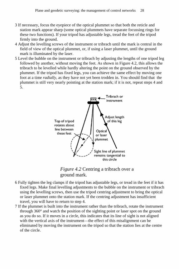
The instrument as a whole may be levelled using a spirit level so that the lsquovertical axisrsquo is in fact exactly vertical the horizontal axis is constructed so as to be accurately perpendicular to the vertical axis though provision is made for adjustment if this becomes necessary Usually a theodolite is mounted on a tripod which allows it to be placed vertically over a known point on the ground such centring is normally carried out using either a plumb bob or an optical or laser plummet Often the instrument is mounted on a tribrach which in turn is mounted on the tripod
A theodolite telescope is an aiming device with four essential parts
Angle measurement 25
1 the object-glass the optical centre1 of which is effectively the foresight of the telescopersquos sighting system
2 the reticle usually a glass diaphragm carrying an engraved cross with a horizontal and a vertical line which is set to be on the optical axis of the telescope and which forms the backsight of the sighting system
3 the internal focusing lens which is used to focus in the plane of the reticle the image of the target formed by the object-glass
4 the eyepiece to magnify the reticle and the image of the target
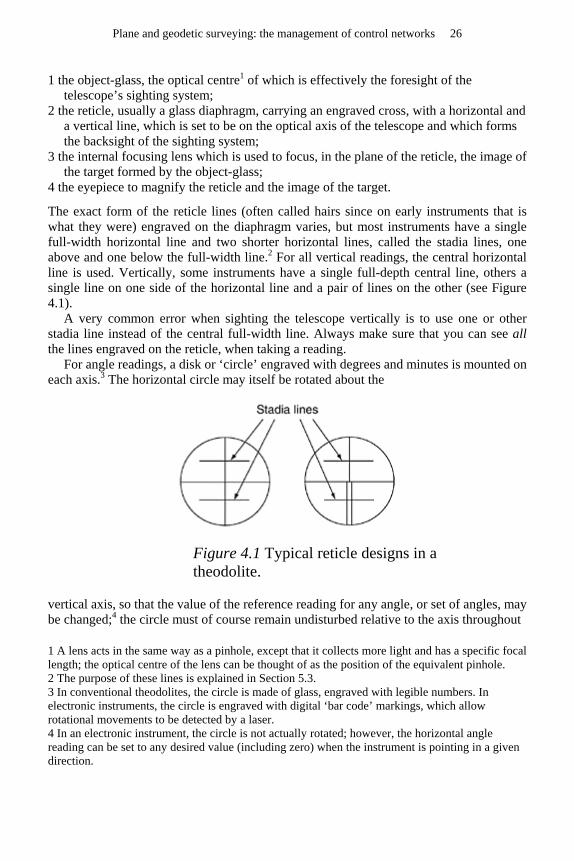
The exact form of the reticle lines (often called hairs since on early instruments that is what they were) engraved on the diaphragm varies but most instruments have a single full-width horizontal line and two shorter horizontal lines called the stadia lines one above and one below the full-width line2 For all vertical readings the central horizontal line is used Vertically some instruments have a single full-depth central line others a single line on one side of the horizontal line and a pair of lines on the other (see Figure 41)
A very common error when sighting the telescope vertically is to use one or other stadia line instead of the central full-width line Always make sure that you can see all the lines engraved on the reticle when taking a reading
For angle readings a disk or lsquocirclersquo engraved with degrees and minutes is mounted on each axis3 The horizontal circle may itself be rotated about the
Figure 41 Typical reticle designs in a theodolite
vertical axis so that the value of the reference reading for any angle or set of angles may be changed4 the circle must of course remain undisturbed relative to the axis throughout
1 A lens acts in the same way as a pinhole except that it collects more light and has a specific focal length the optical centre of the lens can be thought of as the position of the equivalent pinhole 2 The purpose of these lines is explained in Section 53 3 In conventional theodolites the circle is made of glass engraved with legible numbers In electronic instruments the circle is engraved with digital lsquobar codersquo markings which allow rotational movements to be detected by a laser 4 In an electronic instrument the circle is not actually rotated however the horizontal angle reading can be set to any desired value (including zero) when the instrument is pointing in a given direction
Plane and geodetic surveying the management of control networks 26
each set of readings The vertical circle may also be rotated about its horizontal axis so that its zero can be set to the vertical This may either be done manually with the aid of a special spirit level attached to the circle (called the alidade bubble) or (now more commonly) automatically using a damped pendulum
In a traditional theodolite the circles are read optically the reading system incorporates an optical vernier to enable the desired precision of reading to be obtained Readings may usually be estimated to a greater precision than provided by the divisions In a total station or an electronic theodolite the reading is carried out internally and the limit of precision is determined by the manufacturer
Handling
Theodolites whether optical or electronic are delicate and expensive instruments They should be handled with great care Do not jar or knock them or use the slightest force on them Do not touch or rub the lenses if they get wet they can be blotted gently with a tissue
In the field a theodolite is normally put in its container for every move and not carried on its tripod If for short moves in steady conditions it is ever carried on its tripod see that it is secure on the tripod not too far up on its foot-screws and that the clamps are all just tight When carrying the instrument in this way keep it vertical it is not designed to resist stresses at any other angle
When being transported in a vehicle theodolites are vulnerable to high-frequency vibration which can cause large accelerations even at small amplitude It is good practice to transport them in a foam surround or with the container held in the lap of a passenger
Take special care if the instrument has to be set up even temporarily on a hard surface The legs of a tripod are very liable to slip and should be chained together for safety Never leave an instrument unattendedmdashchildren and animals are very inquisitive The instrument should be protected from rainmdashand for precise work from the sun
Setting up centring and levelling
There is no one best way of centring and levelling a tripod The one described below is simple and works well for centring over a station mark on reasonably level ground The ability to set up tripods quickly and accurately is of course necessary when working with targets and GPS receivers as well as theodolites
1 Position the tripod so that its top is roughly horizontal and above the station mark using a plumb bob if desired Note that the top may be levelled by moving the tripod feet tangentially without affecting its position over the mark On sloping ground it is better to have one leg uphill and if the legs are adjustable shorter than the others
2 Attach the instrument to the tripod if it has a detachable tribrach with optical plummet this may conveniently be used on its own for the initial adjustments The instrument or tribrach should be set at the centre of the tripod head with the foot-screws about halfway along their travel The optical or laser plummet will now be roughly vertical and should point within one or two centimetres of the ground mark if it is more than about 5 cm from the mark recheck the orientation of the tripod head and make sure it is approximately horizontal
Angle measurement 27
3 If necessary focus the eyepiece of the optical plummet so that both the reticle and station mark appear sharp (some optical plummets have separate focussing rings for these two functions) If your tripod has adjustable legs tread the feet of the tripod firmly into the ground
4 Adjust the levelling screws of the instrument or tribrach until the mark is central in the field of view of the optical plummet or if using a laser plummet until the ground mark is illuminated by the laser
5 Level the bubble on the instrument or tribrach by adjusting the lengths of one tripod leg followed by another without moving the feet As shown in Figure 42 this allows the tribrach to be levelled while hardly altering the point on the ground observed by the plummet If the tripod has fixed legs you can achieve the same effect by moving one foot at a time radially as they have not yet been trodden in You should find that the plummet is still very nearly pointing at the station mark if it is not repeat steps 4 and 5
Figure 42 Centring a tribrach over a ground mark
6 Fully tighten the leg clamps if the tripod has adjustable legs or tread in the feet if it has fixed legs Make final levelling adjustments to the bubble on the instrument or tribrach using the levelling screws then use the tripod centring adjustment to bring the optical or laser plummet onto the station mark If the centring adjustment has insufficient travel you will have to return to step 4
7 If the plummet is built into the instrument rather than the tribrach rotate the instrument through 360deg and watch the position of the sighting point or laser spot on the ground as you do so If it moves in a circle this indicates that its line of sight is not aligned with the vertical axis of the instrumentmdashthe effect of this misalignment can be eliminated by moving the instrument on the tripod so that the station lies at the centre of the circle
Plane and geodetic surveying the management of control networks 28
8 For targets GPS antennae and self-levelling theodolites the process is now complete If manual levelling is necessary rotate the instrument so that the plate bubble5 (physical or electronic) lies parallel with the line between two foot-screws Centre the bubble by turning these foot-screws equally in opposite directionsmdashyou will find that the bubble follows your left thumb Swing the instrument through 90deg and centre the bubble again by turning the third foot-screw only Return the instrument to its first position and re-centre the bubble if necessary repeating until the bubble is centred in both positions Swing through 180deg note how much the bubble has moved and bring it halfway back Swing through 90deg and bring the bubble to the same position with the third foot-screw The bubble should now remain in this position (not necessarily central) through whatever angle the instrument is swung If it does not repeat the procedure Levelling an instrument really means setting the vertical axis vertical
9 Check that the instrument is still above the station and least to an acceptable degree of accuracy If it is not this indicates a bubble error in the spirit bubble used in steps 5 and 6 This can be rectified by moving the instrument on the tripod so that the sighting point is again over the station and then returning to step 8
Note that the alignment of an optical or laser plummet which is built into a tribrach cannot be checked in the manner described in step 7 even though a misalignment may be present For this reason tribrachs must be regularly serviced and should always be handled with particular care despite their robust appearance
Telescope focusing
The ability to focus a telescope correctly and thus eliminate parallax in the readings is possibly the single most important factor in obtaining good readings from a theodolite (including electronic ones) or from a level A proper understanding of the next two paragraphs is therefore crucial to all surveying
First with the internal focusing lens right out of focus so that no image of the target is visible focus the eyepiece so that the reticle is as clear as possible with your eye relaxed This adjustment depends only on your eyesight and not on the distance to the target once made it should only need to be altered if your eye starts to get tired
For each observation adjust the internal focusing lens so that the image of the target is also sharp This image should then be in the plane of the reticle on which the eyepiece is focused Check this by moving your eye from side to side there should be no relative movement of the target and the reticle ie no parallax If there is any remove it by adjusting the internal focusing lens not the eyepiece Having done this it may seem that the target is no longer exactly in focus in this case refocus the eyepiece so that it is and check that the parallax has disappeared If it has not repeat the procedure above using the internal focusing lens followed (if necessary) by the eyepiece Note that parallax can be neither eliminated nor introduced by adjusting the eyepiecemdashthough it may wrongly appear to be present if the eyepiece is badly adjusted for the observer
5 See the Glossary
Angle measurement 29
Observing the target
Having eliminated parallax the cross hairs must be carefully sighted onto the target Depending on what the target is it might be easier to bisect it with the single cross hair or to lsquostraddlersquo it with the double cross hairs If possible use the same part of the cross hair to sight on each target this will eliminate any errors due to the cross hairs not being exactly horizontal or vertical Always use a part of the relevant cross hair (vertical for horizontal angles and vice versa) which is close to the place where the cross hairs meet
It is helpful to be aware of the precision with which a sighting must be made to achieve a given level of repeatability If a target is 100 m away the cross hairs must be sighted onto it with a precision of plusmn15 mm for a reading which is repeatable to within 5 s If the instrument and the target are removed and then replaced it is unlikely that such a level of repeatability could be achieved at all given the inherent errors of centring over the stations
Repeatability can also be affected by changes in light conditions particularly if the target has a cylindrical or conical shape If the sun shines on one side of the target there is a subconscious tendency to sight the cross hairs onto the sunny side rather than centrally This error known as a phase error disappears when the target is shaded from the sun
Reading the angle
In electronic theodolites and total stations this simply consists of reading the numbers on the display However there are still many older instruments in use with optical reading systems and this sub-section refers to those instruments
Every pattern of instrument is different in the details of circle reading Most will have one or more circle-illuminating mirrors which must be adjusted to obtain even illumination of the circle being observed Most will have an eyepiece with provision for focusing through which the circles may be read In some cases both circles are visible together and a single optical vernier applies to both in other cases a prism is rotated to select which circle is seen and separate optical verniers may be used In each case rotating the optical vernier causes the scale images to move by tilting a parallel-sided glass plate in the light path between the circles and the eyepiece This movement is solely optical and should not be confused with a rotation of the instrument In higher precision instruments the reading system automatically takes the mean of the readings on opposite sides of the circle
Every time before reading the vertical circle level the alidade bubble this ensures a consistent circle reading when the telescope is truly horizontal On many modern instruments and all electronic ones this operation is rendered unnecessary by provision of automatic vertical circle indexing but without that facility it is essential to check the bubble every time when reading vertical angles
Common errors in reading are to read ten minutes or a degree out to read the horizontal circle instead of the vertical circle or vice versa to fail to level the alidade bubble before reading the vertical circle or to misread the optical vernier If you have any doubt on the latter point it is good practice to turn the vernier to zero and make your best estimate of what the angle reading should be Then turn the vernier to take the reading watching carefully what happens in the main display as you do so This always provides
Plane and geodetic surveying the management of control networks 30
the clearest possible indication of how the vernier should be read in any particular instrument
Errors due to maladjustment of the instrument
In a properly adjusted theodolite
1 the line of sight of the optical plummet should be along the vertical axis 2 the trunnion axis should be perpendicular to the vertical axis 3 the line of sight through the intersection of the reticle lines (called the line of
collimation) should be perpendicular to the trunnion axis 4 the horizontal and the vertical reticle lines should be parallel to the trunnion and
vertical axes respectively 5 when the instrument is level and the line of collimation is horizontal this should
correspond with the 90deg or 270deg mark on the vertical circle 6 for convenience in setting up the horizontal plate bubble should be central when the
vertical axis is vertical
These points can be checked and permanent adjustments can be made to all of them All these adjustments are called lsquopermanentrsquo to distinguish them from the lsquostationrsquo adjustments which are made every time the instrument is set up
In addition to the requirements listed above there are others which cannot be adjusted For example
7 the horizontal circle should be perpendicular to the vertical axis and the vertical circle perpendicular to the trunnion axis
8 the centre of the horizontal circle should coincide with the vertical axis and the centre of the vertical circle with the trunnion axis
9 the circles should be accurately graduated 10 there should be no backlash
Tests to check the correct setting of a theodolite may be made and are described in Section 45 If the instrument under test proves to be out of adjustment refer to the makerrsquos handbook for details It is unwise to attempt any permanent adjustment to a theodolite without prior training
Although maladjusted theodolites can be tiresome to use most of their effects on observations are eliminated by the observation techniques which are described in the next section
44 Observations with a theodolite
Principles
It is neither necessary nor possible to ensure that the permanent adjustments described above are always faultless The effects of these and other instrumental imperfections can be almost eliminated and careless mistakes can be avoided by suitable methods of observation
Angle measurement 31
In measuring horizontal angles errors due to maladjustment of the trunnion axis are reversed in sign on changing face6 Such errors are therefore eliminated by taking the mean of circle left (CL) and circle right (CR) measurements
All collimation errors are also reversed on changing face and are therefore eliminated in the same way This applies to both horizontal and vertical angles Since horizontal angles are obtained from the difference of two readings of the instrument the effect of any error in horizontal collimation is in any case eliminated by subtraction unless the points observed are at different altitudes Vertical angles on the other hand are measured from a zero in the instrument itself (the alidade bubble) and measurements taken on one face only are therefore burdened with the whole vertical collimation error It is therefore essential to take CL and CR observations for all vertical angles and for all horizontal angles where high accuracy is required
Errors due to eccentric mounting and inaccurate graduation of the circles are reduced by repeating the observations using a different part of the circle7 but equal numbers of CL and CR observations must be taken
It is common practice to swing the instrument to the right (SR) to observe successive stations when the instrument is circle left (or position I) and to swing it to the left (SL) when it is circle right (or position II) Errors due to any backlash in the instrument are reduced by using the mean of SR and SL measurements by turning the tangent (slow motion) screws clockwise for their final adjustment and by always making the final optical micrometer adjustments in one direction
Besides eliminating certain instrument errors taking the average of a number of measurements is desirable in itself any gross errors in circle reading will be detected and can be discarded Also the ESD (from random causes) of the mean of n measurements varies inversely as
All the above precautions are included in the system of observing and booking suggested below
Practical points
See that there is no play in the hinges between the legs and the tripod If the tripod has sliding legs see that the clamps are tight Focus the telescope and micrometer eyepieces before levelling Start with the tangent screws near the middle of their runs Once the instrument is levelled do not jar the tripod or even rest your hands on it Avoid stepping near the tripodrsquos feet if the ground is soft Swing the instrument by holding the vertical frames which support the telescope not the telescope itself Use the minimum of force on clamping screws
No routine of observation eliminates errors caused by inaccurate levelling of the instrument or inaccurate centring over the station mark
6 Rotating the telescope through 180deg about the trunnion axis then rotating the instrument through 180deg about the vertical axis 7 For an electronic theodolite this will involve physically rotating the instrument on the head of the tripod and re-centring it
Plane and geodetic surveying the management of control networks 32
Recording observations
Most instruments which display readings electronically are also capable of recording them onto a memory card This subsection only applies to instruments where the readings must be recorded manually
Haphazard observation and random booking on loose paper lead to mistakes For speed and accuracy a system is essential The one given here is the result of more than a century of experience in combating human and instrumental error
For efficient working a separate observer and booker are necessary Record all necessary data in an observation book Use a fresh page for each station occupied Book with a ball-point pen or pencil and make your figures neat and clear Do not erase make corrections by drawing a single line through the incorrect figures leaving them legible and writing the correct figures beside or above them A fair copy may be made later on another page if necessary (check carefully for copying errors) but the original pages must not be discarded Notice that single-figure entries are written 06deg 08prime 05Prime not 6deg 8prime 5Prime
The booker fills in the heading and the stations to be observed while the observer is setting up the instrument The observer calls out the readings the booker records them and then reads back what (s)he has written8 the observer then re-checks the reading and replies lsquocorrectrsquo (or not) Do not omit this seemingly pedantic precautionmdashit ensures that there is a lsquoclosed looprsquo between what is visible in the instrument and what is written in the book
It is the bookerrsquos duty to detect inconsistencies (such as excessive discrepancy between CR and CL readings)mdashif one occurs the observer is at once told to check but is not told what is wrong The booker works out reduced angles while the observer is observing the next target Mental arithmetic is both quicker and less error-prone than use of a calculator in the field The booker is responsible for ensuring that the stations are observed in the right order Both surveyors should do their own jobs and not interfere with the other Ideally the observer checks the bookerrsquos arithmetic and both sign the sheet before leaving the station
Remember that in practice the time taken in going to and from a station is large compared with the time actually spent there So take every reasonable precaution to ensure that carelessness does not make a second visit necessary
Horizontal angles
Take at least one full round of observations ie CLSR and CRSLmdashsee Figure 43 In the circle-left position set the horizontal circle reading initially to a random value not to any specific reading9 Swinging from left to right sight on the first point to be observed which will be called the RO (reference object) Swinging right throughout take readings for all the points to be observed from the station Always close the round by re-observing the RO the difference in readings is called the closing error A standard for acceptable closing errors will depend on the instrument in use and on the quality of the work
8 Note that this is not the same as the booker repeating what they have just heard
9 On the first (or only) round of readings the arithmetic is simplified if the horizontal circle is adjusted such that the angle observed for the reference object is just over 0deg
Angle measurement 33
requiredmdasha typical value might be 5 seconds10 If there is an unacceptable closing error all the readings should be discarded and a fresh start made
Figure 43 Booking horizontal angle observations
Change face by transitting the telescope and swinging through 180deg Slightly change the position of the horizontal circle to guard against repeated misreading of the scales and unconscious memories of previous readings Swinging now from right to left sight again on the RO and observe the horizontal circle Swinging left throughout take the readings for all the points to be observed from the station in the order of reaching themmdashie the opposite order from the circle-left readings Close the round again as before
When booking it is always best to write the points for SL in the same order as for SR and to book from the bottom of the form upwards on SL After the first half round and throughout a repeated round the booker is in a position to know in advance what the next reading should be and should ask the observer to check if there is an unacceptable discrepancy
When a round of horizontal angle observations has been completed the booker should enter the mean of the reduced circle-left and circle-right angles in the top part of the 10 Careful selection of a reference object can help in obtaining a small closing error If the object is too far away atmospheric distortions can impair the repeatability of the observation if it is too close the size of the target in the eyepiece will make it hard to sight the theodolite in exactly the same way Remember that one second represents a distance of 05 mm at a range of 100 m
Plane and geodetic surveying the management of control networks 34
right-hand column The bottom part of the same column can be used to record any horizontal or slope distances which are observed
Vertical angles
Always take sets of observations on both CL and CR (see Figure 44) There is no virtue in swinging left or right and there is no RO to close on The horizontal hair may not be quite horizontal so intersect always with the same part of it just to one side of the vertical hairmdashremember that the left-hand side of the reticle on CL becomes the right-hand side on CR
Figure 44 Booking vertical angle observations
The booker records the height of the instrumentrsquos trunnion axis above the station mark Note that without this measurement the angle observations will be uselessIf a target on a tripod is being observed the height of the target above the station will also be needed and can be recorded in the lower part of the right-hand column If some other object is being observed (eg a lightning conductor) the observer makes a sketch in the observation book indicating by an arrow the exact point intersected on the object
Assuming that the instrument measures zenith angles the horizontal will appear as 90deg on CL and 270deg on CR The booker should record next to the CR readings the value obtained by subtracting the reading from 360deg The differences between these and the CL observations can be booked next to the CL readings and should remain nearly constant the constant is zero only if the zero adjustment on the vertical circle is perfect If any difference varies significantly from the norm the booker should demand a check
Angle measurement 35
Finally the top part of the right-hand column should be used to record the accepted vertical angle for each observation namely the average of CL and 360degmdashCR This cancels out any maladjustment of the vertical circle The bottom part of the column can be used to record any slope distances which have been measured andor the heights of observed targets above their stations
Always centre the alidade bubble before taking each reading of the vertical circle
Setting out angles
As mentioned in Chapter 3 it is sometimes necessary to set up a theodolite to sight in a predetermined direction rather than simply to record the direction it is sighted in when observing a target Usually the starting point is a known horizontal angle which must be swung through once a reference object has been observed
With an electronic theodolite the process is then simple Sight on the reference object with the instrument in position I and set the horizontal angle to zero Then swing the instrument to approximately the right direction clamp it and turn the horizontal tangent screw until the required horizontal angle is displayed Markers can then be set up at any point along the line of sight The reference object is then sighted again to ensure that no setting has been disturbed For accurate work this process is then repeated with the instrument in position II and an average of the two sight lines is used
With a conventional theodolite a booking sheet is partially filled before going out into the field with the station name and all columns except lsquoObserved Anglersquo and lsquoMeanrsquo filled in from the known data Once out in the field the reference object is observed in CL and the angle recorded in the usual way The reduced angle of the required direction is then added to this reading and written down in the lsquoObserved Anglersquo column The observer is told to swing the instrument to this angle and does so by first setting the optical vernier to read the appropriate number of minutes and seconds then swinging the instrument and using the horizontal tangent screw until the entire correct reading is shown in the display11 As with the electronic instrument the reference object is then re-observed (and booked) and the process repeated in CR See Appendix F for a worked example in calculating an angle for setting out including the preparation of a booking sheet
45 Checks on permanent adjustments
It is usually impossible to make corrections to permanent adjustments in the field and often unwise to attempt them back at base either unless clear instructions are given in the instrument manual However it is necessary at least to know when an instrument needs to be sent back to the maker for adjustment and to give the correct diagnosis of the problem The following guidelines should assist in this the simpler adjustments are described first
11 A small amount of thought and practice will usually show how this is done on any particular instrument
Plane and geodetic surveying the management of control networks 36
Bubble errors
If there is a significant error in the plate bubble when levelling the instrument up (see Section 43 under Setting up step 8) this can be removed by levelling the instrument carefully then adjusting the plate bubble so that it lies in the centre of its glass In a level instrument with no bubble error the instrument can be rotated about its vertical axis and the bubble will always return to the centre point
If the instrument has been levelled on a tribrach and the cup bubble on the tribrach is not central then this indicates a bubble error on the tribrach Again this can be removed by levelling the instrument and then adjusting the tribrach bubble
If there is a significant difference between the CL and 360degmdashCR readings on a vertical observation this indicates a bubble error in the alidade bubble Putting this right is more advanced The procedure is to make a vertical observation and calculate the mean of the CL and 360degmdashCR readings With the instrument observing the target in CL adjust the alidade bubble until with the bubble central the average reading is obtained Then re-observe on CR and check that 360degmdashCR gives the same angle
Plummet errors
If the plummet (laser or optical) rotates with the instrument it is easy to see whether there is a plummet error by simply rotating the instrument If the line of collimation makes a circle then there is an error this can be removed by keeping the instrument still and adjusting the line of collimation of the plummet to point at the centre of the circle Details of how to do this should be given in the instrumentrsquos manual
If the plummet does not rotate (eg it is fixed to a tribrach) then errors are harder to detect One simple method is periodically to lay the instrument on its side on a bench with the tribrach attached and the vertical axis clamped Sight through the plummet and mark the point on the wall on the line of collimation Unclamp the vertical axis rotate through approximately 120deg and repeat then rotate through a further 120deg and repeat again If the three marks are in different places the plummet has an error Correcting such an error generally requires a special instrument or professional servicing
Reticle errors
Reticle errors should only be corrected by an instrument maker but are relatively easy to diagnose To check the vertical reticle sight on a suitable target with some part of the reticle then rotate the telescope about the trunnion axis and see whether all parts of the vertical reticle align with the target The horizontal reticle is similarly checked by rotating the telescope about the vertical axis
Collimation errors
Collimation errors in the horizontal plane can be detected by sighting on a target at a similar height to the instrument and taking a horizontal angle reading then transitting the instrument and taking the reading again If the two readings do not differ by exactly 180deg then this is due to Collimation error As explained above this error is relatively
Angle measurement 37
unimportant since it largely disappears when one horizontal observation is subtracted from another
Collimation errors in the vertical plane have no real meaning in instruments with an alidade bubble any such error is effectively treated as a bubble error In pendulum instruments any discrepancy between CL and 360degmdashCR vertical angle readings is due to collimation error but is also compensated for by adjusting the pendulum
Trunnion axis misalignment
If the circle-left reduced horizontal angle of an object (reading to the object minus reading to the reference object) differs significantly from the corresponding circle-right angle the most likely cause is misalignment of the trunnion axis particularly if it only occurs when the lines of sight to the two distant objects have different slopes This can be verified by setting up a long plumb line indoors levelling the instrument carefully and sighting the telescope on the bottom of the line then rotating the telescope about the trunnion axis (only) so that the telescope points to the top of the plumb line If the reticle no longer points exactly at the line then the trunnion axis is misaligned and must (usually) be adjusted by the manufacturer
Plane and geodetic surveying the management of control networks 38
Chapter 5 Distance measurement
51 General
Distances may be measured by four methods direct optical electromagnetic or GPS The method used for any particular job depends upon the nature of the ground the range the accuracy the number of distances to be measured the time available and the cost and the availability of the equipment For all but the smallest or largest tasks electromagnetic distance measurement (EDM) is the simplest choice for terrestrial measurement GPS measurements provide inter-point distances over any distance and without the need for inter-visibility but the procedure is somewhat more complex
Before making any measurement it is wise to obtain an estimate of its value by an approximate method to reduce the possibility of gross errors At least three methods are available for this
1 Pacing is used for rough measurements and to check accurate measurements against gross errors Test your natural pace over a measured distance rather than trying to pace metres The accuracy on smooth ground is about 1 part in 50
2 A perambulator is a wheel fitted with a revolution counter and is wheeled along the line to be measured It is more accurate than pacing and is frequently used in measurement for costing of highway repairs
3 If a suitable map is available scaling from it will give a close approximation
52 Tape measurements
Tapes are now mainly used only for the quick measurements of short distances (horizontal or vertical) However they used to be the most accurate method of measuring all distances so their use was developed to a fine art by surveyors in the first part of the twentieth century Tape measurements are subject to the following sources of error
1 inaccuracy in the length of the tape 2 variations in the length of the tape due to changes in temperature 3 variations in the length of the tape due to changes in tension 4 slope (since it is usually the horizontal component of the length that is required) 5 sag on any unsupported spans 6 errors at the junction of tape lengths
For further details of precision taping see Bannister et al (1998)
Surface taping
Fabric tapes made of linen or preferably of fibreglass are used for low accuracy or detail work Steel bands or tapes are more accurate but are easily damaged if kinked or trodden on On smooth ground an accuracy of about 12000 is attainable For the highest accuracy
1 calibrate the tape against a known distance at the same temperature and tension as will be used on the job
2 avoid large changes of temperature by working early late or on a cloudy day 3 use a steady pull ideally by means of a spring balance 4 correct for slope if there are marked changes of gradient measure the slope and note
the length of each section 5 use the longest tape possible if the distance is greater than one tape length 6 take the mean of two measurements in opposite directions
53 Optical methods (tachymetry)
The stadia hairs (Figure 41) on the reticle of a theodolite or level subtend a particular angle α usually 1100 radian Thus if a distant vertical staff is viewed horizontally by means of a theodolite the distance D from the instrument to the staff is given by sα (ie usually 100s) where s is the length of the staff between the two stadia hairs Either an ordinary levelling staff or a specially made tachymetry staff may be used
This method of determining distance is perfectly straightforward when the line of sight is horizontal and modern digital levels also use this principle to measure the distance to their (bar-coded) levelling staffs However it becomes more complex if the line of sight of a theodolite needs to be inclined by some angle to the horizontal in order to observe the staff It is not practicable to hold the distant staff perpendicular to such a line of sight instead it is still held vertical by means of a spirit level and the two readings (plus the vertical angle of the theodolite) can be used to obtain both the horizontal distance to the staff and the height difference between the instrument and the base of the staff
The calculations for this form of tachymetry are tiresome and the technique is now largely obsolete1 In any case the accuracy of vertical staff tachymetry is always limited by the fact that lines of sight defined by the two stadia hairs are differently affected by atmospheric refraction
For distances up to about 50 m a form of horizontal staff tachymetry known as subtense is still sometimes used A special staff called a subtense bar usually 2 or 3 m long is mounted horizontally and at right angles to the direction of view The horizontal angle subtended at the instrument is then measured and the horizontal distance can be deduced by simple trigonometry
1 The formulae are given in Uren and Price (1994) p 144
Plane and geodetic surveying the management of control networks 40
54 Electromagnetic methods (EDM)
Principles
The principle of the method depends on measuring the transit time of an electromagnetic wave which is transmitted along the line and reflected back to the transmitter Some devices transmit a pulsed laser beam and simply measure the time taken for the pulse to be reflectedmdashthis can be done without the need for a special reflector at the far end of the line and is known as a lsquoreflectorlessrsquo system Others use a carrier wave modulated at a known frequency and measure the phase change of the reflected modulation to calculate the distance (see Figure 51) Errors can arise from difficulties in knowing the exact point of measurement within the instrument (a matter of a few millimetres) from inaccuracies in measurement (usually fewer than 10 parts per million) and from variations in atmospheric temperature and pressure along the path of the wave (up to about 20 parts per million if no correction is made)
Figure 51 Electromagnetic distance measurement with a reflector
The reflectors (for those instruments which require them) take the form of lsquocorner cubesrsquo with precisely ground faces so that the radiation is reflected back along the exact path it came along It is important to use only the correct type of reflector with a given instrument since each type has a different lsquodistance constantrsquo depending on the path length of the optics and the density of the glass Neglect of this factor will lead to a systematic error in all measurements
Most modulating EDM devices now use infrared or a visible laser (wavelength a few microns) as the carrier wave modulated at around 1 GHz to give a modulation wavelength of about 30 cm Their range can be up to 30 km Some earlier instruments used microwaves (wavelength a few centimetres) as a carrier and were capable of measuring up to 100 km provided that the end stations were inter-visible (Measurements of this length would now be done by GPS)
The total distance travelled by the modulated wave 2D will be equal to a number of whole wavelengths nλ plus a fraction of a wavelength λδ (see Figure 51) δ is relatively easy to determine by comparing the phase of the reflected wave with that of the transmitted wave Some possible methods are
Distance measurement 41
1 to use a phase discriminator circuit to compare phases directly 2 to shift the phase of the reflected signal by a known amount until it gives a null with the
reference signal 3 to use a digital count of time signals between the reference null and the reflected null
then multiply by the modulation frequency to find the phase difference
The value of n can be found by increasing the modulation frequency by a small fraction and measuring the change in δ Typically the modulation frequency is increased by 1 per cent the resulting fractional change in δ is then multiplied by 100 and rounded down to the nearest integer to give the value of n The change in δ is measured by changing to the new frequency and subtracting the new value of δ from the old value adding one whole cycle in cases where δ appears to have decreased However this method only works properly when n is less than 100 any multiples of 100 would pass undetected Such multiples can however be counted by altering the frequency by 001 per cent (1 per cent of 1 per cent) and again measuring the fractional change in δ Long-range machines may thus need to make several changes of modulation frequency to compute the distance properly
Use of EDM
For short-range work hand-held laser devices can be used to measure distances with an accuracy of around 3 mm without the need for a reflecting target at the far end of the ray EDM systems mounted on tripods are used for high-accuracy (5 parts per million) measurements of distances between say 10 m and a kilometre Longer distances are now generally measured using GPS Although the instruments required for GPS are more expensive they are more accurate (2 parts per million) and they save time especially in rough country and in conditions where the line being measured is obstructed (eg by buildings) or subject to interference by traffic
The basic measurement made by an EDM device is a slope distance between the instrument and the target uncorrected for atmospheric conditions On most instruments it is possible to correct for atmospheric conditions while in the field Temperature and pressure are measured near the instrument (and for accurate work near the target) and a nomogram or lsquoslide rulersquo is provided to convert these readings into a parts-per-million correction which is then entered into the instrument To guard against undetected errors it is wise also to record the temperature pressure and uncorrected distance so that the field correction can be checked back in the office
Some EDMs do not always show the whole of the distance that they are measuring for instance the display might show 2345678 when the distance is actually 12345678 A 10 km error should not easily pass unnoticed but a useful field check is to record the readings obtained with the atmospheric correction set first to +50 ppm and then to minus50 ppm The difference between the two readings when multiplied by 104 gives the approximate distance and any lsquooverflowrsquo in the display will then be detected quite easily
In addition to slope distance most EDMs are also able to calculate the horizontal and vertical distances between the instrument and the target In the case of horizontal distance this has the advantage that the heights of the instrument and the target above their stations do not need to be measured since the horizontal distance between the instrument and the target will also be the horizontal distance between their respective
Plane and geodetic surveying the management of control networks 42
stations (For the other distance measurements to be useful it is of course vital that these measurements are recorded)
To make a calculation of horizontal or vertical distance the microprocessor inside the EDM must know the vertical angle between the instrument and the target This means that the instrument must be carefully aimed at the target it is not sufficient simply to sight it well enough for the radiated signal to be returned Additionally on some detachable instruments a calibration must be set so that the correct vertical angle is displayed The relevant angle is obtained from the theodolite to which the instrument is attached remembering to centre the alidade bubble if necessary
For precise or long-distance work however these calculated distances must be treated with caution A fully accurate lsquohorizontal distancersquo calculation involves knowing the height of the instrument above sea level and both calculations have to make some assumption about how light curves in the atmosphere which may not be valid at the time of the measurement Chapter 11 discusses both of these issues in detail
Distance measurement 43
Chapter 6 Levelling
Levelling is the process of finding the height of a new point or points by comparison with that of an existing point which has been selected as a datum or whose height is already known with respect to some other datum
If the points are close to each other and only their relative heights are needed the simplest procedure is as described in this chapter If however lsquoabsolutersquo heights are required eg for comparison with other points elsewhere in the country then the scheme of levelling should be tied into one or more nearby bench marks1 of known height (The heights of bench marks around Britain are published by the Ordnance Survey but cannot now be fully relied upon as many bench marks are no longer checked regularlymdashsee Chapter 8) Alternatively GPS can be used to find the absolute heights of some of the points but this is also more complex than might be supposed as explained in Chapters 7 and 8
The simple process of comparison is generally done with a level and a staff A level is a telescope mounted on a tripod fitted with cross hairs and a sensitive bubble means are provided for setting the line of collimation (the sighting line) to be exactly horizontal A staff is simply a long ruler and is usually graduated in centimetres
61 Theory
To find the difference in level between two points A and B (see Figures 61 and 62) the observer sets up the instrument at an arbitrary third point I1 An assistant holds the staff vertical with its foot resting on A The observer rotates the telescope about its vertical axis until the staff appears in the
1 Typically a horizontal v-shaped slot cut into a vertical wall They are used by inserting a bracket into the slot and standing a staff on the bracket The bracket is properly called a lsquobenchrsquo hence the term bench markcentre of the field of view sets the line of collimation to be horizontal and then reads the scale of the staff against the horizontal cross hair (distance a in Figure 61) The staff is then moved to B and the observer again directs the telescope on to it obtaining the reading b The difference in level between A and B is then aminusb since if the instrument is correctly adjusted both lines of collimation are horizontal The height of the instrument at I1 does not affect the calculation
Figure 61 Measurements of height differences using a level
Figure 62 Typical line of levelling If the height of a third point C beyond B is required the instrument is moved to I2
between B and C The difference in level between B and C is then found in the same way By repeating this process the difference in level between points at any distance apart can be found
In levelling from a mark at A whose level is known (eg a bench mark) the observation I1A is called a backsight This establishes the level of the instrument (or line of collimation) at I1 The observation I1B is called a foresight Similarly I2B is a backsight I2C is a foresight and so on
A line of levelling is usually started at one bench mark of known height and if possible finished at a different one A long line should be broken into a series of bays of
Levelling 45
between one and five instrument positions Each bay should be lsquoclosedrsquo by being levelled out and then back to its starting point as a check against error Each bay should run between two well-defined markers which can support the staff and will not change in height either a permanent bench mark or a temporary one such as a stout peg It is helpful if the top of the bench mark is convex or if the peg is driven in at a slight angle so that there is a uniquely defined lsquohighest pointrsquo on it which is taken as its height
Figure 62 shows a line of levelling in plan view The first bay runs from a bench mark at A out to C (via B) and then back to A (via D) points B and D are called change points and point C is a temporary bench mark A second smaller bay then runs from C to E and then back to C Finally an lsquoopenrsquo bay is run from E to Z if this gives a height for the closing bench mark which is in good agreement with its published height then there is no particular need to close that bay back to its starting point and the calculated heights of all points in the line can be accepted If the agreement is not good then the bay should be closed if it closes well then it raises the possibility that the first or last bench mark might have subsided since its height was last checked
If the heights of further points are required the staff is held (say) at P and Q and at R and S and readings are taken from I1 and I2 respectively If these intermediate points lie in a straight line and the horizontal distances between them are measured a vertical section of the ground (a level section) can be plotted Observations to intermediate points are called intermediate sights they can be made more quickly than sightings to change points because several sightings can be made from each instrument position but they are also more prone to error because they do not form part of a closed bay
Note the following
1 When the staff is moved the instrument must remain stationary and when the staff remains stationary the instrument must move to guard against a reading error going undetected (If the instrument was not moved from I5 to I6 in the second bay then a misreading to the staff at E would lsquocancel outrsquo to give a bay which appeared to close well yet gave the wrong height for E) The only time when both move is at the start of a new bay or at the end of the job
2 The instrument positions I1 I2 etc need not be on the lines AB and BC etc 3 It is important that there is something definite to stand the staff on at the temporary
bench marks (positions C and E in Figure 62) because both these stations are left and then revisited later in the job By contrast change-point stations B D and F are only visited once so do not necessarily need to be found again later
4 There is no independent check on the heights recorded for stations P Q R and S Any point whose height is critical should form part of a levelling line rather than being taken as an intermediate sight
5 A team of experienced levellers might level from bench mark A to bench mark Z (Figure 62) with a single open bay involving five or more instrument positions If all goes well this is very efficientmdashbut if the bay does not close the whole job must be repeated By contrast a team of novice surveyors would be well advised to make their first bay as small as possible such as the one between C and E
Plane and geodetic surveying the management of control networks 46
62 The instrument
In a tilting level the telescope assembly is carried on a friction-controlled ball joint which can be locked by a locking ring The telescope and a sensitive bubble are pivoted on a horizontal axis and can be slightly elevated or depressed by means of a micrometer screw There is usually a further cup bubble on the body of the instrument On setting up the cup bubble is used to level the instrument approximately by means of the ball joint but no attempt is made to get the vertical axis truly vertical Before each individual reading but after the telescope has been pointed at the staff the telescope is levelled accurately by means of the sensitive bubble and the micrometer screw Slopes can also be set out if the instrument has a graduated ring mounted on the drum of the micrometer screw
In a self-setting or automatic level a stabiliser automatically levels the line of collimation for every sighting The stabiliser consists of one prism fixed internally to the telescope casing and two prisms which are suspended freely as a pendulum within the telescope When setting up a cup bubble on the tribrach is centred to ensure that the telescope axis is not more than plusmn20prime from the horizontal The pendulum is then automatically released from its clamps and the staff can be read at once The makers claim that the pendulum has a repetition accuracy of less than 1 second of arc This type of instrument saves much time when running a line of levels It is however more subject to interference in windy conditions
At normal ranges (up to about 50 m) both types of level permit readings to be estimated quite easily to within 5 mm For work requiring greater accuracy a level fitted with a parallel plate micrometer is used readings may then be taken to the nearest millimetre For higher accuracy still precision levelling can be used (see Section 66)
63 Technique
Many modern levels (especially precision levels) read the staff digitally some of the guidance below is specifically for conventional levels but most is relevant to both types
Set up focus and eliminate parallax as with a theodolite (see Section 43) Level the instrument if necessary as described above Never rest your hands on the tripod while observing
We have assumed that the line of collimation is horizontal when the instrument is levelled This is only true if the instrument is in exact adjustment If the permanent adjustments are not perfect the line of collimation will point up (or down) slightly when the instrument is levelled and all staff readings contain a lsquocollimation errorrsquo Since this error is proportional to the distance of the staff from the instrument it will cause equal errors in sights of equal length Consequently since the carrying forward of the height depends on the difference between backsights and foresights the errors will cancel out if at each position of the instrument the foresight and backsight distances are equal ie I1A should equal I1B in Figure 61 In practice the errors will be kept small if the difference in distances is less than about 5 m
Levelling 47
The line of collimation can also deviate from the horizontal as a result of the tendency of light paths to bend in a vertical plane (see Section 112) The effect of this varies with the square of the length of the line of sight and does not remain constant With ordinary instruments therefore do not take sights longer than 50 m
Particularly when observing on a slope it is very easy accidentally to use one of the stadia hairs (see Figure 41) instead of the main horizontal hair On a typical sight length of 30 m this will introduce an error of approximately 15 cm which should be apparent on checking It is of course preferable not to make the mistake in the first place
On some instruments the staff is seen upside down in the telescope do not correct this by holding the staff itself upside down Before starting work study the scale carefully both with the naked eye and through the telescope Note the difficulty of distinguishing sixes from nines
The staff-holder faces the staff towards the instrument and stands behind it with one hand on each side so as not to hide the scale It is very difficult to hold the staff vertical The observer can see if it is leaning sideways by means of the vertical hair in the telescope and can signal to the staff-holder accordingly but cannot see if it is leaning forwards or backwards The staff-holder should therefore swing the top of the staff slowly towards and away from the instrument passing through the vertical position The observer records the smallest staff reading since this corresponds with the vertical position of the staff
At change points rest the foot of the staff on something firm and convex If necessary drive a peg preferably with a dome-headed nail driven into it so that the foot of the staff is always in contact with the highest point when the staff is vertical If no dome-headed nail is available it is actually preferable to deliberately drive the peg in at an angle so that one corner is uppermost rather than attempting to get the top face of the peg level
64 Booking
Figure 63 shows the method of booking Successive rows of entries on the form refer to successive staff stations the foresight from I1 and the backsight from I2 (both to staff position B in Figure 62) are therefore booked on the same line At each instrument station the height of the line of collimation is obtained from the backsight and then the reduced level of the next foresight is calculated by subtracting the relevant staff reading
The booker who may well also be the observer books each reading in the field book as it is taken using a pencil or ball-point pen Fill in a name for each staff station the entries in the distance columns need only be approximate and can be judged by pacing Do not erase make corrections by drawing a single line through the incorrect figures leaving them legible and writing the correct figures above them A fair copy can be made later on another page if necessary but take care to avoid copying errors and do not destroy the original papers Sign and date the work
Immediately after booking a reading verify it by again looking through the instrument beware of gross errors of a metre or a tenth of a metre Then look at the bubble again to verify that the instrument is level
Plane and geodetic surveying the management of control networks 48
Figure 63 Booking levelling observations
When the bay is complete the booker should add up the total of all the backsights (upward movements) and of all the foresights (downward movements) as shown in Figure 63 The difference between these two quantities should be the same as the calculated difference in height over the bay (in this case 4 mm) If it is not it means there is an arithmetic error somewhere on the booking sheet This check is useful in that it might lsquorescuersquo a bay which appears to have closed badly conversely it will also flag a bay which appears to have closed well as a result of two errors cancelling each other Note though that it does not detect errors in the observations themselves
If the bay has closed acceptably and the arithmetic has been checked the height of all points in the bay can be accepted If desired these heights can also be lsquoadjustedrsquo to their most likely values given any mis-closure in the bay In the case shown point A has closed 4 mm higher than it should the most likely assumption is that there has been a steady upwards lsquodriftrsquo around the bay meaning that the calculated heights for points B C and D should be adjusted downwards by 1 2 and 3 mm respectively The relevant adjustment is shown for point C in Figure 63 as the starting height for the next bay
A further useful check is to add up the total distances for all the foresights and backsights in the bay as shown in Figure 63 In this example the individual backsights and foresights from each instrument position (2528 2731 2025 3134) are all individually within tolerance but there has been a slight systematic bias towards having longer foresights than backsights as shown by the totals If the instrument has a collimation error this accumulating difference will introduce errors into the recorded heights and might in this case explain why the bay has not closed especially well
Levelling 49
65 Permanent adjustments
The permanent adjustments which can be made to a level ensure that the line of collimation is horizontal when the instrument has been levelled Alterations to these adjustments should only be undertaken back at base but it is sometimes useful to check them in the field particularly if the instrument has just been subjected to a heavy impact
Figure 64 lsquoTwo-peg testrsquo for a level
A simple field test called the lsquotwo-peg testrsquo involves driving two pegs into the ground a measured distance x (usually 25 m) apart as shown in Figure 64 Set the instrument up approximately in line with (but not in between) the two pegs and observe to the staff on each peg in turn (readings a and b in Figure 64) Move the instrument to the other end of the line (so that the peg which was near to the instrument is now the far one) and repeat the process to obtain readings aprime and bprime
The slope error of the instrument (in radians) is given by the expression ((bminusbprime)minus(aminusaprime))2x when all distances are expressed in metres and a positive value denotes an upward slope If the absolute value is less than 00001 then the instrument is fine remember that even a value of 00002 would cancel completely if the foresights and the backsights are of equal length and would only produce 1 mm of error if the sight lengths differed by 5 m
For information about tests and adjustments for a particular instrument refer to the makerrsquos handbook (Some instruments have software for computing the results of a lsquotwo-peg testrsquo automatically)
66 Precision levelling
A slower but much more accurate type of levelling is known as precision levelling in which differences in heights are typically read to 001 mm The overall principles are identical to those described above but some extra details are required to achieve the higher precision
1 The staff is not rocked backwards and forwards as described above but is supported by some form of tripod and is made precisely vertical by means of a staff bubble Precision levelling staffs are typically made of Invar to minimise errors caused by thermal expansion
Plane and geodetic surveying the management of control networks 50
2 For maximum accuracy two staffs are used one for the backsight and one for the foresight Since the staffs may not be identical it is essential that bays start and end using the same staff This means that open bays must always have an even number of instrument positions The smallest possible lsquoclosedrsquo bay (from a known benchmark to a new station and back to the known one) will therefore involve four instrument positions so that the same staff is always placed on all the temporary bench marks which are to be used as the starting point of a new bay Thus the bay from A to C and back in Figure 62 would be a valid bay for two-staff precision levelling but the bay from C to E and back is too small
3 The purpose of using two staffs is to allow for changes in temperature which would cause even an Invar staff to change slightly in length The procedure is to read a backsight then a foresight then a second foresight and finally a second backsight The time interval between readings 3 and 4 is made as close as possible to that between readings 1 and 2 Averaging the two results eliminates any temperature effects assuming that both staffs are heating (or cooling) at a constant rate
4 The possibility of cumulative errors from a collimation error in the instrument is more important To guard against this the cumulative totals of distances to the backsights and foresights in a bay are recorded at each step and are kept as close to one another as possible throughout each bay The distances are often measured by tachymetry (see Section 52) but can also be taped for maximum accuracy and for planning the layout of a bay
5 All modern instruments read the staff electronically the staff being marked with a bar coding rather than with numbers (Older instruments had an optical vernier consisting of a piece of glass with high refractive index and precisely parallel surfaces which made them very expensive)
6 The importance of finding firm ground on which to stand the staffs is much greater The staffs are heavy and may settle by a millimetre or more on soft ground while the readings are being taken Even on firm surfaces it is advisable to let each staff rest for a minute or so before taking the first reading
67 Contours
Contours (Bannister et al 1998) are the best method of showing variations in level on a plan they may be thought of as the tidemarks left by a flood as it falls by successive vertical intervals Contouring is laborious the following methods are used
1 The contours are pegged out on the ground with a level and a staff and then surveyed (perhaps by a total station) The staff may have a movable vane set at the same height as that of the telescope above the required contour level to speed its positioning
2 A total station is set up and oriented as for mapping (see Section 33) above a station of known height A detail pole is set to the height of the instrument above its station so that any height difference between instrument and reflector is always the same as the height difference between the station and the foot of the pole The height difference from the station to the required contour is calculated and the pole-holder follows the ground line which gives this height difference with the instrument recording the pole
Levelling 51
position at suitable intervals The contour is then plotted in the same way as other mapping detail
3 The spot levels of points where the slope of the ground changes are taken usually with a total station and the contours are interpolated This is a common method in engineering work it is less accurate than method (2) but much quicker
4 Heights are measured at evenly spaced points on a (x y) grid and the contours are drawn by interpolation This method is particularly useful if the volume of earth in an area needs to be estimated as part of a mass-haul calculationmdashsee Allan (1997) for details Some total stations can lsquosteerrsquo the detail pole to the necessary places and perform the volume calculations
5 Over larger areas contours are most easily plotted by means of aerial or satellite photogrammetry Contours on published maps are now generally plotted by digital photogrammetry (Egels and Kasser 2001)
6 Contours may very effectively be plotted by kinematic GPS (see Chapter 7)
Plane and geodetic surveying the management of control networks 52
Chapter 7 Satellite surveying
71 Introduction
At the time of going to press satellite surveying relies mainly on a system called global positioning system (GPS) which was originally set up as a military navigation aid by the USA in the mid-1980s but which has now become a significant tool for civilian use in general and surveyors in particular Using so-called differential GPS (DGPS) in which data recorded by a receiver at a lsquoknownrsquo station are combined with data recorded simultaneously by a second receiver at a new station which might be 30 km away it is possible to find the position of the second receiver to within about 5 mm The advantage of GPS compared to all earlier methods of surveying is that the two stations do not need to have a line of sight between them This means that national networks of lsquoknownrsquo stations (provided round Great Britain by the Ordnance Survey) no longer need to be located on high hilltops or towers but can for instance be positioned on the verges of quiet roads
72 How GPS works
The GPS system consists of a set of about 24 satellites each of which is in a near-circular orbit about the earth with a period of 12h1 and (therefore) a radius of approximately 26000 km The orbits are all inclined at about 55deg to the plane of the equator and lie in six different planes equally spaced around the equator As a result there are at least four satellites visible at all times everywhere on the surface of the earth unless blocked by terrestrial obstructions In most places and for most of the time the number is greater than this often up to eight or ten
Each satellite broadcasts a set of orbital parameters (the lsquoephemerisrsquo) which allow its position at any instant to be calculated to within about 20 m plus two digital signals whose lsquobitsrsquo are transmitted at very precise moments in time By recording the time at which it receives the digital signal (and knowing the speed of light) a GPS receiver is able to determine how far it is away from the satellite (the lsquopseudorangersquo2) and thus to position itself somewhere on a sphere with a known centre and radius
1 Strictly 12 sidereal hours (a sidereal day being the time for the earth to complete one revolution with respect to the stars rather than the sun) A given constellation of satellites therefore recurs twice each day and about 4 min earlier on each subsequent day
2 The pseudorange of the satellite is the distance calculated by measuring the time when the digital signal is received not allowing for clock errors in the receiver or satellite or for delays caused by the earthrsquos atmosphere
When a second satellite is detected another sphere is calculated and the locus of possible positions for the receiver becomes the circle of intersection between the two spheres A third satellite provides another sphere which will intersect this circle at just two points One of these will typically lie many thousands of kilometres away from the surface of the earth discarding this will give one possible position for the receiver
At this point the principal error in the calculation is caused by the clock in the receiver (the satellites have atomic clocks which are highly accurate) Because light travels at 300 Mms an error of just 1 micros in the receiverrsquos clock will cause an error of 300 m in the calculated radii of all the spheres and thus a large error in the calculated position For this reason a fourth satellite must be detected and a fourth sphere calculatedmdashthe radii of all four spheres are then adjusted by an equal amount such that they all touch at one single point This point is taken as the position of the receiver and the required adjustment in the radii (divided by the speed of light) is taken to be the receiver clock error
If more than four satellites are visible the extra information can be used to provide redundancy in the calculation and the receiver will report a position based on the best fit of the available data
If only three satellites are visible some systems will also provide a lsquotwo-dimensionalrsquo solution by assuming that the receiver is at sea level Figure 71 is a plan view of the earthrsquos surface which shows how three satellites can provide such a 2D solution and correct the receiver clock error The three solid circles are the loci of all points on the earthrsquos surface which are the appropriate distance from each satellite as calculated from the pseudoranges As can be seen there is no one place on the earthrsquos surface which lies on all three circles However if the receiverrsquos clock is running slow this would cause it to underestimate its distance from each satellite advancing the receiverrsquos clock appropriately and recalculating the ranges gives the three dotted circles which do meet at a point
The method described above will enable a single GPS receiver to calculate its so-called lsquonavigationalrsquo position to within about 10 m3 This accuracy can be improved to better than 1 m by leaving the receiver in the same place for an hour or more and averaging the readings Note that these figures have improved significantly since the US military withdrew lsquoselective availabilityrsquo (the deliberate downgrading of the data provided by the satellites) in May 2000mdashearlier literature quotes much higher errors than this
The accuracy of a result is also determined by other factors such as the relative positions of the satellites being observed which will affect the geometry of the computation This effect is referred to as the geometric dilution of precision (GDOP)4 and is expressed as a multiplying factor for the potential error a GDOP of less than 2 is very good but it could rise to 20 or more if all the visible satellites lay in a straight line across the sky Also some cheap receivers only use the so-called lsquocoarse acquisitionrsquo (CA)
3 The accuracy in vertical position is always about 25 times poorer than the accuracy in horizontal position due to the fact that the satellites being observed are always above the plane of the horizon This factor also applies to all subsequent accuracies described in this chapter 4 Sometimes broken down into the lsquoPositional Dilution of Positionrsquo (PDOP) for the accuracy of the positioning on a horizontal plane and lsquoVertical Dilution of Positionrsquo (VDOP) for height information due to the general difference in accuracy of these two calculations mentioned above
Plane and geodetic surveying the management of control networks 54
Figure 71 Clock adjustment in 2D satellite surveying
digital signals from the satellites to compute pseudoranges while others also use the more precise P-code which has a 10-times higher lsquochipping ratersquo5 Finally the best receivers are dual frequencymdashthey receive the P-code from the satellites on carrier waves at two slightly different frequencies6 and can thus estimate (and so largely eliminate) the effect of the earthrsquos atmosphere on the speed of propagation of the signals
The accuracy discussed above refers to the absolute position of the receiver on the surface of the earth and is considerably higher than anything which could be achieved prior to 1980 using astronomical observations However it is insufficient for many engineering purposes which typically require the differences between stations to be known to a few millimetres For this reason surveyors tend to use differential GPS which is described in the next section
73 Differential GPS (DGPS)
The factors which most affect the accuracy of a single high-quality GPS receiver are errors in the positions of the satellites errors in the satellite clocks and the effects of the earthrsquos atmosphere on the speed at which the satellite signals travel If two such receivers are within say 10 km of each other the effects of these factors will be virtually identical and the difference vector in their positions will be correct to within a decimetre or two If
5 The rate at which bits are transmitted in the satellitersquos binary signal 6 These are known as the L1 frequency (157542 MHz) and the L2 frequency (122760 MHz)
Satellite surveying 55
the distance between the receivers is greater than this the accuracy of a simple difference calculation is degraded by the fact that the two receivers will be observing the same satellites but from somewhat different anglesmdashso that the positional and clock errors of the satellites will have slightly different effects on the calculated positions of the two receivers This is overcome however by a more sophisticated form of post-processing which requires one of the receivers to be at a known position and then effectively corrects the positions of the satellites using the data recorded by that receiver Ultimately the accuracy of DGPS is limited by the fact that signals to the two receivers are passing through different parts of the earthrsquos atmosphere and will suffer different propagation effects This constrains the overall accuracy of DGPS to about 2 mm for every kilometre of separation between the two receivers (ie 2 parts per million) up to the point where the two receivers can no longer see the same satellites
The final precision of DGPS is achieved by measuring the phase of the carrier wave onto which the P-code is modulated The chipping rate of the P-code is 1023 MHz which means the bits in the signal are about 30 m apart By contrast the L1 carrier wave has a frequency of 157542 MHz and thus a wavelength of about 19 cm Interpolation of the phase of the carrier signal will yield a differential positional accuracy of a few millimetres provided it has been possible to use the P-code to obtain a result to within 19 cm beforehand If not the carrier phase cannot be used because of the uncertain number of whole wavelengths between the satellite and the receiver The attempt to determine the number of whole carrier wavelengths is called lsquoambiguity resolutionrsquo It is usually possible to resolve ambiguities when the receivers are up to 20 km apart given a good GDOP and enough observation timemdashand it is usually unwise to attempt it7 if the receivers are more than 30 km apart because of the unknown differences in atmospheric delays along the two paths Note therefore that the term lsquoDGPSrsquo can imply a wide range of relative positioning accuracy from about 2 mm up to 2 dm or so
A final factor which is important at the top level of precision is lsquomultipathrsquo ie the reception of signals which have not come directly from the satellite but which have bounced off (for instance) a nearby building this can cause errors of up to half a metre in the calculated position of the receiver For this reason differential GPS stations should always be sited well away from buildings and large metal objects In particular differential GPS cannot be relied upon to produce accurate results in the middle of a construction site it is much better practice to use DGPS to fix control stations around the edge of the site and then to use the more conventional surveying methods within the site
Base stations for differential GPS
As explained above if two receivers are more than about 10 km apart the accurate computation of a DGPS difference vector requires that the absolute position of the base station is known to an accuracy of about 1 m If a completely lsquolocalrsquo co-ordinate system
7 Processing the data under these circumstances may yield a seemingly plausible solution which might in fact be incorrect by one or more whole wavelengths Software from responsible suppliers will warn a surveyor against using results unless the statistical likelihood of their correctness is high Even then however it is impossible to guarantee that the calculation has yielded the correct result
Plane and geodetic surveying the management of control networks 56
is to be used for a project it is perfectly acceptable to base the whole system on a point which has been fixed as a navigational solution provided it is observed for long enough to fix it to that accuracy All difference vectors built out from that point will be of high accuracy and all points fixed using those vectors will also have an absolute accuracy of less than 1 m so in turn they can be used as base points for further vectors
Often however it is necessary to tie in new GPS stations to a countryrsquos national mapping system This can be done in three different ways using three different types of lsquoknownrsquo station
1 Passive stations Most countries including the UK provide a network of stations with known (and published) co-ordinates These are often sited on roadsides or other public places and so can be occupied without obtaining permission Using one or (preferably) more of these stations as base stations will tie all new stations into the national co-ordinate system
2 Active stations In addition to passive stations several organisations maintain lsquoactiversquo base stations at known positions These record GPS data which are subsequently published (usually via the Internet) and which can be downloaded for post-processing in conjunction with data recorded by a roving receiver This system allows users with only one GPS receiver to carry out differential GPS and increases the productivity of users with more than one receiver The format of the data is normally Receiver-INdependent EXchange (RINEX) which is the standard format for passing GPS observations between different manufacturersrsquo equipment
Before using this service it is wise to check the frequency at which the chosen active station records its observations (typically once every 15 s) and to set your own receiver to record at the same frequency this simplifies and improves the quality of the subsequent post-processing Be prepared also to return from recording your own observations only to find that they cannot be used because the active station was not working that day The fact that the base and the roving station may be using different types of antenna may also cause problems as they will have different offsets The documentation for the post-processing software should explain how to allow for thismdashbut any error in inputting this information will potentially go undetected As a check download some further data from another active station with yet another antenna type and check that the two differential vectors produce consistent results
3 Broadcasting stations An emerging service in several countries is the permanent installation of GPS receivers which act as base stations and broadcast their data via short-wave radio to any nearby GPS receiver Surveyors who have paid to use the service and who have suitably equipped receivers can use this information to show their position to within a centimetre or so in real time (see lsquoReal time kinematicrsquo) This system is also used at airports enabling DGPS to be used as a precision landing aid
Satellite surveying 57
74 Using DGPS in the field
Differential GPS relies on the same satellites being observed at the same time by the two receivers If one receiver is recording while the other is not those observations will be unusable There are a number of ways of using DGPS in practice depending on the size and purpose of the survey The principal ones are as follows
1 Static When the two receivers are more than about 15 km apart it is necessary for them to remain simultaneously in position for an hour or more recording observations every 15 s or so The time period allows the satellites to move through significant distances and for a larger number of satellites to be observed by both receivers simultaneously-and the number of observations ensures a good chance of resolving ambiguities if that is desirable or of obtaining a well-averaged result if it is not Static survey is usually used for the establishment of new control stations in an area well away from any existing lsquoknownrsquo stations
2 Rapid static If the distance between the receivers (the lsquobaselinersquo) is less than 15 km the observing time can be reduced because the atmospheric effects will be nearly identical for each receiver The time required depends on the length of the baseline the number of satellites the GDOP and the algorithms in the receiver The instruction manual should give advice on the observation time required failing that about 10 min is probably prudent in most cases With lines shorter than 5 km five or more satellites and a GDOP of less than 8 5 min will probably be adequate
3 Stop and go In this procedure the roving receiver makes a rapid static fix at its first station and is then moved to other stations while maintaining lock on the satellites which it is observing Subsequent points can then be fixed very quickly in about 10s This procedure is suitable for collecting the positions of a large number of points in open country but if fewer than four satellites can be tracked at any point a new lsquochainrsquo must be started by doing another rapid static fix
4 Kinematic This procedure also starts with a rapid static fix8 after which the roving receiver moves continuously recording its position at regular time intervals (perhaps as frequently as once per second) As with stop and go satellite lock must be maintained at all times This technique is typically used for surveying boundaries and other line features
5 Real time kinematic (RTK) If two suitably equipped receivers are less than about 5 km apart and have a near line of sight between them it is possible for the base station to transmit its position and observations to the roving receiver using a short-wave radio The roving receiver can then carry out the DGPS calculations in real time and display its current position in the GPS co-ordinate system (see Section 76) If a suitable transform has also been downloaded the roving receiver can also display its position
8 Increasingly the processing software is capable of resolving phase ambiguities even while the roving receiver is moving but a user would normally wish to wait at the first point until enough readings had been taken to resolve ambiguities in order to fix the position of that point
Plane and geodetic surveying the management of control networks 58
in the local co-ordinate system Using RTK the operator of the roving station can be confident that enough observations have been recorded to resolve ambiguities while still out in the field and so can carry out rapid static or stop and go procedures more quickly In addition RTK can be used to lsquoset outrsquo a station at a predetermined location albeit without any independent check of its accuracymdashsee the next section
Whichever method is used there are some fundamental rules which should be followed when using GPS to maximise the chances of accurate results
1 Avoid using satellites which are at a low elevation (less than 15deg above the horizon say) as the signals from these satellites will be greatly affected by atmospheric effects due to their long path through the atmosphere Most surveying GPS systems will ignore all such satellites by default
2 Avoid working close to large buildings In the northern hemisphere a building to the south will tend to block out visible satellites completely while buildings anywhere else may cause multipath effects The combination of these two effects is potentially disastrous
3 Working beneath the canopy of a tree can also block the signals from satellites When working in stop and go or kinematic mode just passing briefly beneath the canopy of a tree can cause loss of lock resulting in greatly reduced accuracy for all subsequent readings in the chain
4 Most GPS processing software allow a surveyor to check in advance what the GDOP of the satellite constellation will be at the time when it is planned to take readings This simple precaution can avoid long periods wasted out in the field waiting for the GDOP to improve to the point where useful readings can be taken
Building a network of stations
Usually the goal of a GPS survey is to establish the precise location of a number of fixed stations in the field Logically this is achieved by fixing the position of an lsquounknownrsquo station with respect to a lsquoknownrsquo one using DGPS The unknown point then becomes known and can be used (if required) as the basepoint for further DGPS vectors to find the position of other unknown points
In practice there is no need for the sequence of observations to follow this logical order it is simply necessary for the results to be processed in that order Nor is it necessary for one receiver always to act as the base station while the other always acts as the roving station it is quite permissible for them to lsquoleapfrogrsquo each other taking the role of base and rover respectively as a chain of points is visited
It is however important to plan in advance what readings need to be taken and then to plan a sequence of movements for the receiver(s) to ensure that they are in fact taken A clear written record of what observations have been taken by each receiver (together with a note of the height of the antenna above the station) will also greatly simplify the subsequent processing and archiving of the data A form for this purpose is given in Appendix G
Satellite surveying 59
75 Redundancy
Attentive readers of this book will be aware of the need for redundancy in all surveying measurements Although properly post-processed differential GPS results are the average of many individual lsquoobservationsrsquo there is still the possibility of a systematic error (one receiver not being in exactly the correct place for example) which will cause an erroneous result
The straightforward solution to this is to establish each new station by setting up DGPS vectors from at least two lsquoknownrsquo stations A gross error will then quickly be detected if the two vectors do not meet at almost the same point Furthermore the post-processing software supplied with the GPS equipment will probably contain a least-squares adjustment facility which will find a lsquobestrsquo position for each unknown point based on the co-ordinates of the known points and the DGPS vectors which have been collected Clearly collecting more lsquoredundantrsquo vectors will result in a more accurate result with a smaller chance of an undetected gross error
If time is limited redundancy can be achieved by conducting a GPS lsquotraversersquo similar to the conventional traverse described in Chapter 2 The first unknown point is fixed with respect to an initial known station and is then used to fix the next point This then becomes the base station for the third point etc finally finishing on another known point (preferably not the one where the traverse started) If the position of the final point as calculated by the traverse is in good agreement with its known position it can be assumed that all has gone well This approach does however have two drawbacks
1 It is possible that a satisfactory result masks two errors which have cancelled out eg the incorrect entry of an antenna offset when the antenna is used an equal number of times as lsquobackrsquo station and lsquofrontrsquo station along the traverse
2 If an error is detected it will not be possible to determine the leg in which it occurred and another visit to the site will be necessary It may therefore be wiser to take more redundant readings on the first visit since this could allow a faulty reading to be eliminated without another site visit
Ultimately though all surveyors should be aware that GPS has the tendency to be a lsquoblack boxrsquo science in which a large amount of information is collected and may not be fully checked by the user There is a distinct possibility of some overall systematic error in the collection or processing of GPS information (the inappropriate use of a program the wrong settings in a transformation or a software bug perhaps) which might cause a completely undetected error in the final result If absolute confidence is required in a set of new stations for a major project it is strongly advised that a few checks are made by conventional surveying techniques The re-measurement of some distances using EDM for example is generally less accurate than DGPSmdashbut will clearly show if a scaling error has inadvertently been introduced into the GPS results This is simply the modern equivalent of the old practice of pacing a distance which has been measured by tape to check that the number of complete tape lengths has not been miscounted
Height information obtained from DGPS needs particular care partly because it is less accurate anyway and partly because of the nature of the co-ordinate system used by GPS which is described in the next section If the heights of stations fixed by GPS are to be relied upon it is strongly recommended that the relative heights of some stations in the
Plane and geodetic surveying the management of control networks 60
network are checked by conventional means such as levelling (Chapter 6) or by reciprocal vertical angles (Chapter 12) Again these conventional methods may be less accurate than GPSmdashbut if any discrepancies are too large to be accounted for by their inaccuracy then there is clearly a problem with the GPS results
76 Processing GPS results
The ephemeris information of all GPS satellites and thus the navigational position of a single GPS receiver is expressed in terms of a co-ordinate system called WGS849 In its basic form WGS84 is defined as a set of right-handed orthogonal axes with its origin at the centre of mass of the earth the x- and y-axes lying in the equatorial plane and the z-axis passing through the North Pole
The exact orientation of the axes was originally set up to coincide with the equatorial plane as defined by the Bureau Internationale de lrsquoHeure at the very start of 1984 with the x-axis passing through the lsquoprime meridianrsquo (approximately the Greenwich meridian) at the same instant Subsequently the orientation of the axes has been defined such that the mean drift of all the tectonic plates on the earthrsquos surface is zero with respect to them
Figure 72 Cartesian and geographical co-ordinate systems
9 World Geodetic System 1984
Satellite surveying 61
The xyz-axes are complemented with a biaxial ellipsoid10 of defined shape11 (close to the overall shape of the earth) with its centroid at the origin and its axis of rotational symmetry lying along the z-axis as shown in Figure 72 This gives a more natural way of defining a point on the earthrsquos surface in terms of its latitude (the angle ) longitude (the angle λ) and its height above the ellipsoid (h) These two co-ordinate systems are called Cartesian and geographical respectively and are explained in more detail in Chapter 9
This is a properly lsquoglobalrsquo co-ordinate set for a GPS but unfortunately it does not suit any single country particularly well for two principal reasons
1 The positions of lsquofixedrsquo points on the earthrsquos surface (eg concrete blocks set into the ground) do not have constant co-ordinates in the WGS84 system because of continental drift In the UK and northern Europe this drift is in excess of 2 cm per year in some parts of the world it is up to 10 cm per year
2 The heights reported by GPS measurements are heights above the surface of the WGS84 ellipsoid which is in general not parallel to the surface of zero height (the lsquoGeoidrsquomdashsee Chapter 8) in any particular country Thus the difference in ellipsoidal heights between two stations measured by differential GPS might be quite different from the difference in their orthometric heights as measured using a level A naiumlve surveyor might be surprised to find that water can flow from a point with a low WGS84 height to another point with a greater WGS84 height
To make proper use of GPS results it is therefore necessary to understand about the relationship between WGS84 and heighting and mapping co-ordinate systems used within a particular country
In Europe the first step was to take the accepted WGS84 co-ordinates of a number of ground stations around Europe (all on the Eurasian tectonic plate) in 1989 and to establish a co-ordinate system or lsquoframersquo similar to WGS84 which is defined to be the best fit to those published co-ordinate values This co-ordinate frame is called ETRF8912 and effectively eliminates the first of the two problems described above by slowly drifting away from WGS84 The ETRF89 co-ordinates of all immovable ground stations in the UK remain constant and the definitive ETRF89 co-ordinates of several GPS control points around the UK are published by the Ordnance Survey By setting up a base station on one or more of these control points and using differential GPS the precise ETRF89 co-ordinates of any other point can be found13
ETRF89 is simply a lsquoframeworkrsquo of points which form the practical realisation of a larger lsquosystemrsquo called ETRS89 This system defines that the WGS84 ellipsoid should be used to convert ETRS89 Cartesian co-ordinates (x y z) to geographical co-ordinates (λ
) Amongst other things it also predicts the rate at which the ground stations are moving with respect to the WGS84 system and thus provides a method for defining other ETRFs in the future
10 The 3D shape created by spinning an ellipse about its minor axis 11 The dimensions of this and other commonly used ellipsoids are given in Appendix A 12 European Terrestrial Realisation Frame 1989 13 Although the ETRF89 co-ordinates of the base station will differ by a few centimetres from its WGS84 co-ordinates this difference is too small to affect the accuracy of the DGPS calculation described in Section 73
Plane and geodetic surveying the management of control networks 62
For surveying work it is usually necessary to transform the ETRS89 co-ordinates (geographical or Cartesian) into suitable local mapping co-ordinates There are two principal types of transform which can be set up to do this
1 The lsquoone-steprsquotransform If the transform is only to be used over a small area of land (up to 10 km square say) a localised transform can be set up by quoting the 3D positions of three or more14 points in the local co-ordinate system (ie easting northing and height in the countryrsquos mapping system or a site co-ordinate system) and also in ETRS89 Provided the points are well distributed over the area in which the transformation is to be used15 the errors inherent in this type of transform are small by comparison with the errors inherent in differential GPS All other points whose positions have been found with respect to ETRS89 can then be processed through the transform to find their local co-ordinates
2 The lsquoclassicalrsquo transform In all mapping projection systems there is a scale factor which varies from place to place by which a distance measured on the ellipsoid must be multiplied before it can be plotted on the projection (see Chapter 9) The lsquoone-steprsquo transform can accommodate this but assumes that the scale factor is constant over the area for which the calculated transformation is to be used If the area is too big for this assumption to be valid it is necessary to use the so-called lsquoclassicalrsquo or Helmert transform which first transforms the ETRS89 (x y z) co-ordinates into equivalent (x y z) co-ordinates of whatever ellipsoid has been used for the mapping projection (Airy in the UK) These are then converted to geographical co-ordinates (latitude and longitude) for the relevant ellipsoid (see Chapter 8) and appropriate projection system is applied to give map co-ordinates of easting northing and height above the local ellipsoid (see Chapter 9) Then data must be available to convert the height above the local ellipsoid into a height above the geoid (also known as an lsquoorthometricrsquo height) A complete lsquoroadmaprsquo of this process is shown in Figure 73
As with the one-step transform a classical transform can be established if the co-ordinates of three or more points are known both in the ETRS89 system and also in one of the local systems A classical transform will produce valid results over a much larger area than a one-step transform In order to set it up however it is necessary to know the co-ordinates of three or more points in both systems ie in WGS84 (or a realisation of WGS84 such as ETRS89) and also with respect to the ellipsoid used for the local mapping projection system If the map co-ordinates and projection method are known the latitude and longitude on the local ellipsoid can easily be calculated but to find the ellipsoidal heights from the orthometric heights the separation between the geoid and the local ellipsoid must be known at each point Likewise to obtain orthometric heights from GPS data using a classical transform it is necessary to have a method for converting a height above the local ellipsoid to an orthometric height at any point within the area of interest
14 If more than three points are available a least-squares fit will be used to generate the best transformation between the two co-ordinate systems 15 The accuracy of the transform will be compromised if the points lie in a near-straight line This will not matter however if the area of the survey is itself a near-straight line eg a pipeline or road
Satellite surveying 63
Figure 73 Roadmap for converting between co-ordinate systems
Both transforms allow for full 3D rotation and translation to convert from one co-ordinate system to the other In addition they both make provision for a scale factor to be introduced to give the best possible lsquofitrsquo between the two systems This can be useful but the scale factor must then be applied to any distance which is to be converted from a lsquorealrsquo distance to one in the local co-ordinate system or vice versa In the case of the classical transform this scale factor is additional to any scale factor implied by the projection method so when setting up classical transforms it is often better to insist that the transformational scale factor is kept at unity
It is clear from the descriptions above that the lsquoone-steprsquo transform is the easier one to use provided the area of application is sufficiently small Exact details of how to set up and apply both these types of transform will be found in the user manual for the post-processing software provided by the GPS supplier
77 Further details of GPS
The present GPS system consists of three so-called segments
1 The control segment This comprises the computing power necessary to track the satellites and to predict their orbits ahead for 24 h using a highly sophisticated model of the earthrsquos gravitational field Tracking is done by a network of six tracking stations around the world which then feed information back to the main control centre in Colorado The orbital predictions are uploaded to the satellites every 24 h
2 The space segment This comprises the 24 satellites each of which receives and stores its predicted orbit and transmits this and other information tohellip
3 The user segment The rest of the GPS community
Plane and geodetic surveying the management of control networks 64
Despite the huge expense of deploying and maintaining the satellite network an expense borne by the US Department of Defense the US Government is currently committed to maintaining a level of free civilian access to the system
The GPS signal
Each of the satellites transmits signals on two carrier frequencies both derived from a fundamental oscillator running at 1023 MHz The two frequencies are L1 157542 MHz or 154 times the fundamental and L2 122760 MHz or 120 times the fundamental As explained earlier the purpose of having two frequencies is to enable the correction of errors caused by ionospheric effects
Each satellite also transmits a number of digital signals modulated on the L1 and the L2 signals It is important to realise that since the signal strength is so weak in relation to the background noise and all the satellites transmit at the same frequencies a particular transmission can only be recognised by knowing in advance what code is modulated onto it and thus what to lsquolistenrsquo for16 These codes are
1 The coarse acquisition or CA code a pseudorandom17 bit sequence of length 1023 bits different for each satellite and with a repetition time of 1 ms The CA code enables the receiver to distinguish between transmissions from the different satellites It is used in low-cost navigation receivers as the basis for measurements The bits are released at a rate of 1023 Mbs (the so-called lsquochipping ratersquo derived from the fundamental oscillator) so one bit corresponds to a distance of approximately 300 m The CA code hence gives access to what is known as the standard positioning service
2 The precision or P-code also a pseudorandom bit sequence but at ten times the frequency of the CA code with a chipping rate of 1023 Mbs The cycle length of the complete P-code is in excess of 37 weeks and each of the satellites is allocated a different lsquoweekrsquo so that each satellite effectively has its own P-code The code for all satellites is reset every week at midnight on saturdaysunday Contrary to what is said in much of the early literature the P-code is not restricted to military use in itself The generation algorithm is and always was in the public domain However its use can sometimes be denied to the civilian user by the substitution of an encrypted form of P-code known as the Y-code The encryption algorithm is not publicly available Encryption is known as anti-spoofing or AS since its purpose is to prevent an enemy force from setting up a lsquospoofrsquo transmitter which could make the US military receivers indicate false positions
3 The navigation message a digital data stream running at 50 bs This message contains amongst other things orbital information (called the ephemeris) for the transmitting satellite repeated every 30 s and less precise lsquoalmanacrsquo information to tell the receiver which other satellites are likely to be visible Reception of the almanac for the whole constellation takes 125 min
16 Somewhat similar to hearing onersquos name spoken on the other side of a room full of people talking 17 The bit pattern in the code looks as though it is random and would pass most lsquorandomnessrsquo testsmdashbut it is in fact entirely predetermined
Satellite surveying 65
The navigation message and the P- or Y-code are carried on both L1 and L2 frequencies whereas normally the CA code only appears on L1 This makes acquisition of L2 signals difficult when AS is present but the manufacturers of survey receivers have developed ingenious ways of avoiding the problem
Ionospheric effects
As mentioned earlier these can be estimated by comparison of pseudoranges measured on both L1 and L2 frequencies (It should be noted that the ionosphere delays the code parts of the signals but advances the carrier phase by an equal amount) Single frequency receivers thus have greater difficulty in resolving phase ambiguities since they have no estimate of the ionospheric effect that being derived from the different delays in the code transmissions on the two frequencies
GPS time
The fundamental measure of time used in the world is called universal co-ordinated time (UTC) The length of a UTC second is defined by the decay rate of caesium To ensure that midnight continues to occur in the middle of the night on average lsquoleap secondsrsquo are occasionally introduced into UTC so that the final minute in a year often lasts for 61 s instead of 60 s18
GPS time is measured in weeks and seconds from 00000 on 6 January 1980 It is established by averaging the clock readings from all the satellites19 and from a ground-based master clock and is then steered so that its seconds increment within one microsecond of UTC seconds However GPS time has no leap seconds so now runs ahead of UTC by more than 12 s A further complication is that the lsquoweek counterrsquo is only 10 bits long so lsquorolls overrsquo to zero after 1023 weeks This occurred for the first time in August 1999 causing problems in many receivers It will happen again in March 2019
78 Other satellite positioning systems
GPS has never been the only satellite positioning system other systems such as Transit preceded it and Russia has a system called Glonass which has remained mainly a military system
To enhance the accuracy of GPS in certain areas and to provide a backup system in the event of GPS failing or being withdrawn several countries have already developed regional augmentation to the GPS (and Glonass) signals using geostationary satellites
18 Prior to this definition the length of a second was defined as 186400 of the time taken for the earth to rotate once with respect to the sun averaged over the yearmdashhence the term Greenwich Mean Time Although this avoided the problem of leap seconds it meant that no one knew exactly how long a second was until the end of the year 19 Because the satellites are moving at nearly 4000 ms around the earth there is a noticeable effect on the four atomic clocks they each carry due to relativity
Plane and geodetic surveying the management of control networks 66
These include WAAS in the United States MS AS in Japan and EGNOS (European Geostationary Navigation Overlay System) in Europe EGNOS is due to come online in 2004 and will deliver positional accuracy of better than 5 m from a single receiver throughout Europe
In addition the European Union has planned an entirely independent satellite system called Galileo which will further enhance navigational accuracy as well as provide a number of other services (eg for search and rescue) In particular it is intended that there should be no common mode of failure between GPS and Galileo
Galileo is planned to come online in 2008 and will consist of 30 satellites in circular orbits inclined at 56deg to the equator there will be three orbital planes with ten satellites equally spaced on each plane The orbital radius will be 30 Mm giving an orbital period of about 14 h
Galileo is conceptually quite similar to GPS and will also work by measuring the time taken for signals to travel from a satellite to a receiver
However it will broadcast signals on three different frequency bands (1164ndash1215 MHz 1260ndash1300 MHz and 1559ndash1591 MHz) which should significantly improve the calculation of atmospheric delays In addition some of the signals will incorporate an integrity check intended to guard against false indications of position
Galileo will bring two major benefits to the surveying community
1 It will improve accuracy and reduce observation times by providing more satellites GDOPs of greater than 6 will cease to occur
2 It should perform noticeably better than GPS in built-up areas due to the integrity checks in the signals
On the other hand Galileo is planned as a commercial venture in which the users will pay for the deployment and maintenance of the system In particular it is intended that commercial users (ie surveyors) should pay for the enhanced positioning services that they will need by means of access-protection keys on their receivers
Satellite surveying 67
Chapter 8 Geoids and ellipsoids
81 Definition of the geoid
The purpose of engineering surveying is to find the relative positions of points in three dimensions so a 3D co-ordinate system is needed to record the findings The one absolute direction which can always be found is lsquouprsquo using nothing more sophisticated than a plumb bob For this reason alone it makes sense to define one axis of the co-ordinate system in the upward direction The other two axes can then be conveniently defined to form an orthogonal set with the first axis and can be thought of as lying at right angles to each other on the surface of a bowl of water held at the foot of the plumb bob
Extended over a hundred metres or so this water surface is virtually a flat plane1mdashso a simple Cartesian co-ordinate system with the z-axis pointing upwards is ideal for small-scale work When extended part or all of the way round the world however the surface (which is actually a surface of constant gravitational potential energy) is not flat and lsquouprsquo is not always in the same directionmdashso a more elaborate co-ordinate system is needed for larger surveys
There are infinite number of surfaces of constant gravitational potential around the earth each at a different height The one used by surveyors worldwide is called the geoid and can be thought of as the surface defined by the sea level around the world in the absence of wind or tidal effects
The geoid is thus easy to define but its exact position in any part of the world can be quite hard to find In Great Britain a local realisation of the geoid was created by observing the mean tide height at Newlyn in Cornwall between 1915 and 1921 and establishing a physical datum mark at the resulting average point2 All so-called orthometric heights in Great Britain are measured with respect to this datum In fact the shape and position of the geoid is steadily changing due to effects such as continental drift and global warming Thus all countries tend in practice to define their own geoid by measuring heights from a fixed datum close to the geoid rather than using a common geoid
1 Even over this distance the direction of the vertical will alter by about 3 seconds 2 This is called lsquoOrdnance Datum Newlynrsquo or ODN
82 The need for an ellipsoid
The exact shape of the geoid is complex and irregular It dips in the middle of deep oceans and rises in mountainous areas Overall however it corresponds fairly closely (to within 100 m or so) to a biaxial ellipsoid3mdashthe 3D shape achieved by rotating an ellipse about its minor axis A useful co-ordinate system for large surveying projects is therefore the so-called lsquoGeographicalrsquo system in which the positions of points are defined in terms of latitude ( ) longitude (λ) and height (h) above an earth-shaped ellipsoid as shown for point P in Figure 81
Note that
1 The line PR is the line passing through P which is perpendicular to the surface of the ellipsoid at the place where it passes through it It does not in general pass through the centre of the ellipsoid
2 When the sizes of the ellipsoidrsquos major and minor axes (a and b in Figure 81) are known the geographical co-ordinates of P ( λ h) can
Figure 81 Defining a point using geographical co-ordinates
3 Sometimes called a spheroid in the literature
Geoids and ellipsoids 69
be converted into (x y z) co-ordinates in a Cartesian system having its origin at the centre of the ellipsoid the z-axis lying along the minor axis of the ellipse and the x-axis passing through the zero (Greenwich) meridian Section 84 explains how (and why) this is done
3 The distance h is called the ellipsoidal height It is not a height in the true sense since the geoid is not exactly ellipsoidal in shape
Historically there was no obvious reason for every country to use the same ellipsoid for mapping purposesmdashso different countries each chose an ellipsoid whose surface corresponded closely to the geoid within their area of interest These local ellipsoids each have different shapes and different positions and orientations with respect to the earthrsquos crust Moreover since the position of each ellipsoid is defined in terms of fixed points in the country which adopted it the relationship between them is continually changing because of continental drift
In Great Britain the Airy 1830 ellipsoid was adopted for mapping purposesmdashthis corresponds quite closely to the geoid over the British Isles being about 1 m above it along much of the east coast and about 3ndash4 m below it along the west coastmdashsee Figure 82 By contrast the separation between the geoid and the ETRS89 ellipsoid varies between 45 and 56 m across Britain as shown in Figure 83 Note that the geoid has been defined in slightly different ways in these two figuresmdashbut the difference is negligible compared to the difference between the two ellipsoids
The fact that the surface of the geoid is not parallel to any particular ellipsoid gives rise to two effects which need to be considered
1 If a plumb bob was hung from the point P in Figure 81 it would not lie exactly along the line PR Moreover the neighbouring surfaces of constant gravitational potential are not even parallel to each othermdashso if the string of the plumb bob was made longer it might point in yet another direction These differences however are negligible for all practical purposes
2 More importantly the difference in ellipsoidal heights between two points on the earthrsquos surface will not be the same as the difference in their orthometric heights (ie their heights above the geoid or the height difference found by levelling) To convert between the two it is necessary to know the lsquogeoid-ellipsoid separationrsquo (usually denoted N and defined as positive if the geoid lies above the ellipsoid) at each of the two points In Figure 84 it can be seen that the difference in the orthometric heights of two points (H2mdashH1) is given by
H2minusH1=(h2minush1)minus(N2minusN1)
(81)
Plane and geodetic surveying the management of control networks 70
Figure 82 The British geoid on the Airy ellipsoid
The second of these effects becomes even more noticeable as a result of GPS which has made it increasingly attractive for countries to use the WGS84 ellipsoid (or a derivative of WGS84 such as ETRS894) in place of their lsquolocalrsquo ellipsoids Because WGS84 was designed to provide a global lsquobest fitrsquo with the earthrsquos geoid it is neither as close nor as parallel to the geoid as the local ellipsoid of any particular country In other words N is larger and apt to vary significantly between one place and another as shown in Figure 83
4 See Section 76 for the definition of the WGS84 and ETRS89 co-ordinate systems
Geoids and ellipsoids 71
Figure 83 The British geoid on the ETRS89 ellipsoid
Plane and geodetic surveying the management of control networks 72
Figure 84 Difference between orthometric and ellipsoidal heights
83 Orthometric heights and bench marks
The procedure for determining orthometric heights in Britain mentioned briefly at the start of Chapter 6 can now be explained in greater detail
During the first half of the twentieth century a number of fundamental bench marks (FBMs) were established across Britain by precise levelling from the Newlyn Datum A large number of additional bench marks were subsequently established using the nearby FBMs as reference heights To find the orthometric height of any point in the UK a surveyor would simply level from the nearest BM as described in Chapter 6 Effectively the shape of the British geoid was defined by the physical positions and published heights of these bench marks
FBMs consist of elaborately constructed underground chambers in geologically stable places containing the actual bench mark These are topped off with a small pillar which protrudes just above the ground and which carries a domed brass marker whose height is published and upon which a levelling staff can be placed The top mark is then normally used for levellingmdashbut if it is destroyed it can be rebuilt and its height re-established from the FBM below By contrast ordinary BMs are cut into walls of buildings etc and are much more liable to subsidence and destruction
The task of regularly checking all BMs throughout the UK and publishing any changes in height was a massive one and has now been abandoned by the Ordnance Survey because of the advent of GPS The positions and heights of BMs are still published but they must now be used with increasing caution especially in areas liable to subsidence
Instead of defining the British geoid through a network of BMs the Ordnance Survey now does so by means of a numerical model called OSGM025 This was constructed by comparing the orthometric heights of several FBMs around the country (measured as describe above) with their ellipsoidal heights in the ETRS89 system (measured by
5 This supplants OSGM91 used for the production of Figure 83
Geoids and ellipsoids 73
differential GPS) to give known values for the separation between the British geoid and the ETRS89 ellipsoid at various places around Britain These values were incorporated into an interpolator which is then able to calculate a value for the geoid-ellipsoid separation at any other place6
1 The British geoid as defined by the new method is slightly different from the ones defined by the old method (eg SN70) except at the FBMs used to construct OSGM02
2 Neither definition yields the exact shape of the true geoid passing through the Newlyn Datum as both are based on many further measurements and approximations which potentially contain errors The inaccuracies inherent in the new definition are however small by comparison with the errors inherent in making practical use of it
This change has been prompted by the fact that an ellipsoidal height can now be found anywhere in the country to within about 1 cm using differential GPS One receiver is placed at the point whose height is required another is placed on a GPS passive station with known ETRS89 co-ordinates or data are downloaded from a nearby lsquoactiversquo station After recording data for about 24 h (necessary because of the comparative inaccuracy of height readings from GPS) the ETRS89 co-ordinates of the new station are computed The OSGM02 model then provides the orthometric height of the station
To find differences in heights over a short distance it is more accurate and often quicker to use levelling techniques (fixing one height by GPS if orthometric heights are also required) than to fix both heights independently by GPS However the best accuracy which can be expected even from precise levelling is about 2radicd mm where d is the distance between the two points in kilometresmdashso if the two points are more than 25 km apart it is more accurate (and certainly much quicker) to find their relative heights by means of GPS
84 Transformations between ellipsoids
Because points on the earthrsquos surface can be expressed in terms of different Cartesianellipsoidal systems there is often a need to convert a pointrsquos co-ordinates from one system (A say) to another (B) This is particularly the case when GPS information (which is measured in the WGS84 system or perhaps in ETRS89) needs to be combined with information defined in terms of a local ellipsoid such as Airy 1830
First the ( λ h) (ie latitude longitude height) co-ordinates of the point in ellipsoidal system A are converted into the corresponding (x y z) co-ordinates as shown in Figure 81 This requires the shape parameters of the ellipse in question which are normally given in terms of the semi-major axis a and the reciprocal of flattening7 r The semi-minor axis b can then be obtained (if required) from the expression
(82) 6 Note that 7 The flattening f of an ellipse is defined by
Plane and geodetic surveying the management of control networks 74
and the eccentricity e of the ellipse by
(83)
The first step is to calculate the distance QS in Figure 85 Calling this distance d it is straightforward (but a bit tedious) to show that
(84)
Figure 85 Conversion from geographical to Cartesian co-ordinates
Geoids and ellipsoids 75
and also that the distance QR is given by
(85)
The Cartesian co-ordinates of P are then easily obtained by the following formulae
(86)
(87)
(88)
The next step is to transform the (x y z) co-ordinates of P in system A into corresponding co-ordinates in system B which we will term (xprime yprime zprime) This transformation consists of a translation and a rotation to accommodate the fact that the two ellipsoids have different centres and orientations with respect to each other Sometimes though a scale factor is also defined as part of the transform This is fundamentally illogical since 1 m in system A should equal 1 m in system B albeit in a different orientation The purpose however is to allow for the fact that the sets of fixed markers which still define some ellipsoids are not the exact distance apart that they have been defined to be due to the difficulty of measuring accurate distances at the time when the size of the ellipse and the co-ordinates of the markers were defined
Any change in orientation in three dimensions can be thought of as a rotation of a given magnitude about an axis lying in a given direction The vector re can be used to define this rotation with the unit vector e=[ex ey ez]T defining the direction of the axis and r the magnitude of the rotation in radians The scalar values of rex rey and rez are the so-called Euler angles which define the change in orientation and are more simply written as rx ry and rz
The transformation caused to the point (x y z) by a rotation through an angle r about the axis e passing through the origin is given by
(89)
where c=cos r and s=sin r When r is in radians and is very small (as it usually is between ellipsoids)8 this formula can be simplified by assuming that cos r=1 and sin r=r The transformation then becomes
(810)
8 Note that if a one-step transformation is being established (see Section 76) the rotation will not be small Then the full expression given in equation 89 must be used
Plane and geodetic surveying the management of control networks 76
The origin shift t and the scale factor s (which is usually expressed as a fractional increase or decrease so must have 1 added to it) can now be incorporated into the transformation Doing this and substituting the simpler format for the Euler angles gives
(811)
It is important to realise that the equation above is not actually being used to move the point at (x y z) Rather it is being used to re-express the pointrsquos co-ordinates in terms of a different (xprime yprime zprime) set of axes which are not exactly aligned with the original (x y z) axes
Finally the transformed (xprime yprime zprime) co-ordinates are converted back into ( λprime hprime) co-ordinates on ellipsoid B Inspection of equations 86ndash88 will show that this is not as straightforward as converting from ( λ h) to (x y z) but it can be done as follows
The value of λprime can be found by dividing equation 87 by equation 86 and rearranging to give
(812)
remembering that if xprime is negative then λprime lies between 90deg and 270deg W of Greenwich
is most easily found by iteration Equations 86 and 87 can be combined to give
(813)
Since h is generally much smaller than d a good first guess for is to assume that hprime is zero and use equation 813 to write
(814)
Likewise we use equation 88 to obtain
(815)
Combining these gives the first guess for
(816)
This value is then used in equation 84 to obtain a first guess for dprime (with n=1)
(817)
Geoids and ellipsoids 77
Equation 88 can now be rewritten as
(818)
and combined with equation 813 to obtain an improved guess for
(819)
Equations 817 and 819 are now used repeatedly to get improved values of dprime and respectively until the changes in are within the accuracy required Finally hprime is
obtained from equation 813 using the final values for dprime and
(820)
A worked example of this process is given in Appendix C The following points are useful when applying the transform
1 Be sure to use the given parameters correctly in equation 811 The values of rx ry and rz must be in radians and the value of 1+s should be very close to unity (The given angles are often quoted in seconds of arc and the scale factor is often quoted in parts per million)
2 Remember that if (say) millimetre precision is required from the conversion this is about one part in 1010 compared with the (x y z) co-ordinates of the point All calculations must be done to ten significant figures and lsquodouble precision arithmeticrsquo should be used in computer programs
3 It is useful to have at least one point whose position is already known in both systems to test that the transform has been set up correctly before further points are transformed
4 The reverse transform can be obtained by changing the signs of the shifts rotations and scale factor quoted for the forward transform Note that this reverse transform is not the exact inverse of the original transform matrix so any transformed points will not return exactly to their original positions the resulting position errors will be of the order of δ2RE where δ is the movement caused by the rotational part of the transform and RE the earthrsquos radius (638times106 m) This is because the transform matrix is the approximate version shown in equation 810 rather than the exact (and conformal) version given in equation 89 The resulting errors are usually negligible but might become significant for Euler angles larger than one second
85 ETRS89 and the International Terrestrial Reference System
A common application of ellipsoid transformations is the conversion of co-ordinates between the realisation of WGS84 on a particular continent (ETRS89 in Europe) and the
Plane and geodetic surveying the management of control networks 78
International Terrestrial Reference System (ITRS) which is the lsquodefinitiversquo realisation of WGS84 on the earthrsquos surface ITRS is a method for generating reference frames by means of a lsquobest fitrsquo to a number of points around the world but since these points lie on different continents they are continually moving with respect to one another by quite substantial amounts Applying the method thus gives rise to a series of so-called International Terrestrial Reference Frames (ITRFs) which are published from time to time by the International Earth Rotation Service (IERS) At the time of writing the most recent one is ITRS2000
ETRS89 was based on the accepted ITRS co-ordinates of the ETRF stations in Europe at the start of 1989 but then slightly amended by subsequent and more accurate re-measurement of the relative positions of the stations Since 1989 the drift of the Eurasian tectonic plate has caused the two systems to move steadily further apart
As a result the official transform between ETRS89 and ITRS2000 quoted by IERS has a time element built into it The time which must be used is the period (in years) between 1 January 1989 and the date for which the ITRS co-ordinates are required Applying this transform allows surveyors from different continents to combine their data on a common lsquobest-fitrsquo framework at any given point in time
The parameters for this transform together with the dimensions of several commonly used ellipsoids are given in Appendix A
Geoids and ellipsoids 79
Chapter 9 Map projections
91 Categories and properties of projections
Chapter 8 has shown that it is useful to express the 3D positions of points near the earthrsquos surface in terms of latitude longitude and height above an ellipsoid of defined shape This system gives a precise and straightforward definition of any pointrsquos location in terms of parameters (east north and up1) which are convenient to use everywhere around the world
It is often necessary to record the positions of points boundaries and natural features such as coastlines on a mapmdashand this too is usually done by showing the (east north) positions directly on a flat 2D projection and (where necessary) the heights by means of contour lines etc The complication which arises is that the surface of any ellipsoid including a sphere is doubly curved and therefore cannot be developed (ie unwrapped) to form a planar projection One solution is to project the surface features of the ellipsoid directly onto a plane alternatively they can be projected onto a developable surface such as a cylinder or cone which is then developed to give a planar projection In each case the resulting projection can subsequently be scaled down to give a map of a useful size
It is not possible to project a doubly curved surface onto a planar or developable surface in such a way that the scale of the projection is unity (or any other constant value) at all places Thus all such projections involve some degree of distortion on the resulting map except at certain points or along particular lines By varying the exact method of projection it is possible to manipulate the changes in scale so as to avoid some aspects of distortion on a map but usually at the expense of increased distortion in other respects In particular there are three important properties which maps may have they are as follows
1 A conformal projection manages the scaling effects such that at any point on the projection the scale in all directions is the same2 Such maps are also orthomorphic which means that small shapes on the ground (buildings etc) are shown as the same shape on the map The result of this is that the angles at which two lines cross on the earthrsquos surface are preserved exactly on the map However the shortest distance over the ellipsoid between two distant points (a geodesic) does not in general plot as a straight line on the map
2 An equal area projection manages scaling such that if the scale at a point is increased in one direction then it is reduced in another Thus the area of any feature on an equal area map (eg a state) is preserved exactly subject to the quoted scale of the map
1 Not exactly lsquouprsquo as defined by a plumb bob as the ellipsoid is not necessarily exactly parallel to
the geoid 2 This scale is called the scale factor and is greater than 1 if the size on the projection is greater
than the size on the ellipsoid
However the shape of the area will not be preserved exactly and at any point on the map the scale in one direction (eg north-south) will generally differ from the scale in any other direction (eg east-west) Small circles drawn on the surface of the earth would plot as ellipses of the same area on the projection but with greater eccentricity in places where the distortion of the projection is higher
3 In an equidistant projection the scale of the projection is maintained at unity along a particular set of geodesics Equidistant projections are normally azimuthal projections (see below)mdashthen the scale is preserved along all geodesics radiating out from the central point of the projection These geodesics also plot as straight lines so that distances from the central point to any other point on the map can be measured directly However all other geodesics will plot as curved lines on the map
No projection can have more than one of these properties over an extended area and some have none of them preferring instead to strike a compromise between them Conformal projections are generally preferred for surveying purposes because angles measured in the field (with total stations etc) can be plotted directly onto the map
Apart from these properties there are three important classes of projection depending on the surface onto which the initial projection is made These are described below
Azimuthal projections
At any point on the earthrsquos surface the azimuthal plane is defined as the plane passing through the point and lying normal to the vertical at that point An azimuthal projection involves projecting the surrounding region onto that plane this can be done so as to give a conformal equal area or equidistant projection
An azimuthal projection at the North Pole (Figure 91) would show the North Pole as a central point with lines of constant latitude (known as parallels) appearing as concentric circles around it If the whole world was projected the South Pole would appear as the outermost circle3 Meridians would appear as radial lines crossing the parallels at 90deg
Azimuthal projections can be made at any point on the earthrsquos surface and have the advantage of having distortion which is zero at the central point and increases as a function of distance from that point They are thus suitable for mapping countries or regions which are approximately circular in shape However Azimuthal projections at points other than the Poles would normally treat the earth as a sphere rather than an ellipsoid to simplify the projection algebra This makes them unsuitable for high-precision surveying work on a large scale (over 100 km say) because it is inappropriate to model the geoid as a spherical surface over large areas
3 The South Pole could not be shown at all if the projection was conformal as the scale factor would be infinitely large
Map projections 81
Cylindrical projections
The classical cylindrical projection can be visualised as wrapping a sheet of paper round the earthrsquos equator to form a cylinder and projecting points on the earthrsquos surface out onto it as shown in Figure 92 The projection angle α is a function of the latitude of a given point the function can be defined so as to give an equal area projection or a conformal projection
Figure 91 Azimuthal projection
Figure 92 Cylindrical projection When the paper is unwrapped the resulting projection shows parallels as straight
horizontal lines and meridians as straight equally spaced vertical lines This type of
Plane and geodetic surveying the management of control networks 82
projection has no distortion on the equator and low distortion nearby and so is particularly suitable for mapping tropical countries
The transverse form of a cylindrical projection involves wrapping the sheet of paper round a meridian (called the central meridian) rather than the equator as shown in Figure 93 (Actually this is not strictly a cylindrical projection since meridians on an ellipsoid are not exactly circular) Transverse cylindrical projections give maps which have no distortion on the central meridian and low distortion nearby and so are suitable for countries at any latitude which lie in a predominantly north-south direction (eg the British Isles)
Oblique cylindrical projections also exist in which the earth is treated as a sphere rather than an ellipsoid and the cylinder touches its surface round a great circle other than a meridian or the equator Such projections are useful for mapping countries which lie along such a line
Conical projections
Conical projections are generally made onto a cone whose axis passes through the North and South Poles and whose surface passes through the surface of the earth along two parallels known as the standard parallels Points on the earthrsquos surface are projected onto the cone which is then developed to give a map of the shape shown in Figure 94 As in an azimuthal projection the lines of constant latitude are concentric circular arcs and the meridians are straight radial lines at right angles to the arcs The spacing of the parallels can be arranged to give a projection which is conformal equal area or equidistant (with the central pole as the reference point)
Figure 93 Transverse cylindrical projector
The resulting projection has no distortion of shape or scale on the standard parallels and low distortion near to them A suitable choice of standard parallels can thus give a minimum-distortion projection of a country running in a predominantly east-west direction such as the United States of America
Map projections 83
Figure 94 Conical projection
The angle between neighbouring meridians and thus the shape of the developed map depends on the shape of the initial cone (which in turn depends on which two parallels are chosen as the standard parallels) At one extreme the cone becomes a flat circular disc and the result is an azimuthal projection as described above At the other extreme the cone becomes a cylinder either touching just at the equator or cutting parallels which are equally spaced north and south of itmdashthis of course is a cylindrical projection
92 Individual projections
There are over 60 different types of projection in use around the world usually selected to give the least overall distortion in the context of the size shape and location of the area which is to be mapped It is beyond the scope of this book to describe all of these to a useful level of detailmdashthe reader is referred to Bugayevskiy and Snyder (1995) in the first instance Four projections will however be described in further detail as they are of particular interest to surveyors around the world
The Lambert conformal projection
This is a conical projection as described in Section 91 and as its name suggests the spacing of the parallels is arranged so as to give maps which are conformal An ellipsoidal shape and two standard parallels must be specified to define the projection fully The scale factor of the map is unity on these two parallels between them it is less than unity (meaning that projected features would be smaller than life size on a full-sized projection) and outside them it is greater than unity It rises to infinity at the pole which is furthest from the apex of the cone so this pole cannot be shown on the map
The USA is typically mapped by means of the Lambert conformal projection the parallels at 33deg N and 45deg N and the GRS80 ellipsoid4 are normally used when mapping
4 See Appendix A for the dimensions of this ellipsoid
Plane and geodetic surveying the management of control networks 84
the entire country Individual states are also mapped using this projectionmdashbut with different standard parallels to minimise the distortion in their particular area of interest
As with all conformal projections there is only one family of geodesics which project as straight lines in this case the meridians All others will project as curves and allowance for this must be made for large surveys as described in the next section
Note that there are several other types of lsquoLambert projectionrsquo As stated above cylindrical and azimuthal projections can be seen as special cases of conical projections so can be classed as Lambert projections and Lambert projections are sometimes plotted as equal area projections rather than as conformal ones In addition the azimuthal versions do not always have the North or South Pole as their central point but may instead use any other point specified by its latitude and longitude In these cases the earth is treated as a sphere rather than as an ellipsoid to simplify the subsequent computations
The Mercator projection
The Mercator projection is a conformal cylindrical projection with the cylinder touching the earth around its equator The scale factor of the projection is a function of latitude only it is unity on the equator and rises to infinity at the poles Normally therefore a Mercator projection only shows latitudes up to about plusmn80deg
This projection has the useful property that a straight line drawn between two points on the map cuts each meridian at the same angle this is a so-called lsquorhumb linersquo which a navigator could set as a constant compass bearing to travel between the two points However rhumb lines are not generally the shortest path between two points and the corresponding geodesics between the same two points plot as curved lines on the map
A major drawback of this projection is that above latitudes of say 40deg the scale factor of the map starts to change significantly with increasing latitude This makes Arctic countries look much larger than they really are by comparison with tropical ones and also means that in a country such as Great Britain the north of Scotland is plotted at a noticeably larger scale than the south of England
The transverse Mercator projection
Also known as the Gauss-Lambert projection this is a conformal version of the transverse cylindrical projection described in Section 91 (see Figure 93) and is defined by specifying the shape of the ellipsoid a central meridian and the value of the scale factor along it (known as the central scale factor)
Great Britain is mapped using a transverse Mercator projection for the reasons described in Section 91 The Airy 1830 ellipsoid5 is used together with the 2deg W meridian being the meridian which most nearly runs up the middle of the country
If the central scale factor for Britain was set to unity on the central meridian it would rise to about 10008 at the extreme east and west of the country For making a map of the British Isles it is desirable to have the scale factor as near to unity as possible over the whole of the mapping area so the central scale
5 See Appendix A for the dimensions of this ellipsoid
Map projections 85
factor is actually defined to be about 099966 on the central meridian rising to about 10004 at the extreme east and west of the country This can best be visualised as having the original cylinder lying slightly inside the central meridian and cutting through the earthrsquos surface about 180 km on either side of it features between the two cutting lines are reduced in size when projected onto the cylinder and those outside them are enlarged
The universal transverse Mercator (UTM) projection
This projection system provides a low-distortion projection of the whole world and consists of separate transverse Mercator projections of 60 so-called zones (lsquosegmentsrsquo) of the earthrsquos surface lying between lines of constant longitude Each zone covers a 6deg band of longitude with zone 1 having its central meridian on the 177deg W meridian and subsequent zones following on in an easterly direction Thus the central meridian of zone 29 is 9deg W that of zone 30 is 3deg W and that of zone 31 is 3deg E (These are the three zones which are of relevance to the UK) The central scale factor of each zone is exactly 09996
The UTM projection is normally used in conjunction with the international 1924 ellipsoid whose details are given in Appendix A However it is sometimes used in conjunction with other ellipsoids (eg WGS84) so it is wise to check which ellipsoid has been used before processing UTM data
UTM is a useful global projection systemmdashbut it is not a universal panacea because a region which does not wholly lie within 6deg of one of the 60 central medians cannot be properly plotted on a single TM zone Possible solutions to this are
1 to extend a zone slightly so as to include the whole region 2 to create a non-standard TM projection by using a different central meridian 3 to butt two or more neighbouring UTM projections together in the region of interest
Options 1 andor 2 are feasible solutions to the problem a UTM can readily be extended by 500 km on either side of the central meridian so any area spanning up to 1000 km from east to west can be handled with negligible loss of accuracy
Option 3 is inappropriate for surveying purposes As shown in Figure 95 the boundaries of neighbouring zones (known as lsquogoresrsquo) are not straight so can only touch one another at a single latitude Thus any other point on the common boundary would map to two separate places on the projection and lines would lsquokinkrsquo as they passed from one zone to the next
6 The exact value at the central meridian is 09996012717
Plane and geodetic surveying the management of control networks 86
Figure 95 Universal transverse Mercator projection
93 Distortions in conformal projections
Distortions on a conformal map only become obvious to the naked eye about 45deg away from the central meridian (or from a standard parallel in the case of a conic projection) However some distortion of shape or scale is present over virtually the entire projection so must be taken into account by surveyors
The two important aspects of distortion in a conformal projection are (a) that the line of sight between two points does not plot as a straight line and (b) that the scale factor varies from point to point Methods for dealing with both of these are described below
Curvature of geodesics
When the line of sight between two points is projected onto the surface of the ellipsoid the resulting line is called a geodesic which is defined as the shortest line on the surface of the ellipsoid between the two points in question
On a perfect sphere geodesics are all great circles with their centres at the centre of the sphere On an ellipsoid things are more complex some geodesics lsquosnakersquo slightly between their two endpoints However the geodesics between two points with the same longitude always lie on the (elliptical) line of longitude between the points and for other points less than about 30 km apart the difference between a geodesic and a great circle is negligible
In conformal conical projections the only geodesics which remain exactly straight are meridians in transverse cylindrical projections they are the central meridian itself and those geodesics which cross the central meridian at right angles All others appear to bulge in the direction of higher scale factor when projected (The angles which these
Map projections 87
lines make with other lines they meet or cross are however exactly the same as on the earthrsquos surface)
The effect of this distortion can be seen by reference to Figure 96 which is a transverse Mercator plot of three stations A B and C If a theodolite is set up on station B and stations A and C are observed the two lines of sight made by the theodolite will plot as the curved lines on the figure Because these lines in general lsquobulgersquo by different amounts the angles they make at B with the corresponding straight lines on the projection (labelled lsquotrsquo) are differentmdashso the angle between the two lines labelled lsquoTrsquo (ie the horizontal angle observed by the theodolite) will be slightly different from the angle ABC as calculated by trigonometry from the (x y) co-ordinates of A B and C
The angles between the lsquoTrsquo lines and their corresponding lsquotrsquo lines at a point can be calculated if the shape of the ellipsoid the projection parameters and the positions of both endpoints are known this calculation is called a lsquo(tminusT)7 correctionrsquo For the British National Grid (and by extension for UTM projections) the calculation is described fully in Ordnance Survey (1950) pp 14ndash16
For distances of less than 1 km which lie within 200 km of the central meridian the (tminusT) correction is negligibly small However over longer distances or on conformal projections which cover larger areas it must be taken into account In Figure 97 for example the 7deg W meridian should ideally project as a straight line between the latitudes 50deg N and 58deg N since it is a geodesic in fact it cuts the 54deg N latitude at a point which is about 800 m west of the intercept made by a straight line drawn on the projection between the same endpoints The (tminusT) correction for this line is about 12 minutes at each end of the ray
Figure 96 Curvature of geodesics on a transverse Mercator projection
7 Pronounced lsquotee to teersquo
Plane and geodetic surveying the management of control networks 88
The (tminusT) calculation is tedious to carry out by hand and would normally be done by computer in the context of adjusting horizontal angle observations A surveyor should ensure that any adjustment software which works with projected (as opposed to geographical) co-ordinates takes account of this correction before using it for a large-scale survey8
Scale factor distortions
The local scale factor of a projection must be taken into account whenever distances in the field are converted to projected distances Distances are routinely measured to just a few parts per million so a local scale factor which lies outside the range 0999999ndash1000001 will make a significant difference The scale factor of a projection is defined as (projected length true length) on the full-size projectionmdashso any distance measured on the ellipsoid must be multiplied by the local scale factor before it can be treated as a distance on a conformal projection (Slope distances or lsquohorizontalrsquo distances measured above or below the reference ellipsoid require additional processing as explained in Chapter 11)
In all conformal projections the scale factor S is a function of the central scale factor (if any) and the distance from the point or line(s) of zero distortion For short lines (lt10 km) the local scale factor will be reasonably constant along the whole length of the line so a single scale factor can be appliedmdashideally this would be obtained at the midpoint of the line
For longer lines the scale factors should be found at both endpoints and at the midpoint of the line a mean scale factor can then be estimated using Simpsonrsquos Rule ie
(91)
The formula for calculating the scale factor at a point depends on the details of the projection The formula for calculating scale factors in all transverse Mercator projections is given in Appendix D
94 Grids
Having developed a planar projection from one of the projections described in Section 92 it is often convenient to superimpose a right-handed rectangular Cartesian grid system onto it This enables the plan position of any point on the map (or ground) to be identified by an (x y) co-ordinate The Y-axis is usually defined to lie along a meridian (the central meridian in the case of a transverse Mercator projection) and the x and y co-ordinates are then known as eastings and northings respectively
8 LSQ provided with this book does so for UTM and British National Grid projections
Map projections 89
Figure 97 The British National Grid The grid system is positioned by specifying the latitude and longitude of a reference
point which is called the true origin of the system However if the true origin is given the co-ordinates (00) it may lead to some points having negative co-ordinates which can be undesirable The true origin may therefore be given a different set of co-ordinates these are known as lsquothe false co-ordinates of the true originrsquo9 and the point which
9 Or sometimes just the lsquofalse co-ordinatesrsquo
Plane and geodetic surveying the management of control networks 90
thereby acquires the co-ordinates (00) is known as the false origin In the case of the British National Grid the unit of length is the metre and the true
origin has latitude 49deg N and longitude 2deg W with false co-ordinates (400000E minus100000N) This places the false origin somewhere to the south-west of the Scilly Isles All points in the British Isles thus have positive grid co-ordinates and all points on the mainland can be specified to an accuracy of 1 m using two six-figure co-ordinates
In Britain this grid is sometimes broken down into 100 km2 with two-letter designators for approximate referencing purposes as shown in Figure 97 thus the co-ordinates of the Cambridge University Libraryrsquos tower (a second-order control point in OSGB36) can be quoted to the nearest centimetre as (54416676E 25840919N) or to the nearest kilometre as TL4458
UTM grids are likewise defined in metres and the true origin for each zone is where the central meridian crosses the equator The false co-ordinates of each true origin are (500000E 0N) for the northern hemisphere so that all points in the zone have positive eastings and northings For the southern hemisphere the false co-ordinates are usually set to (500000E 10000000N) so that the northings of these points are positive also To distinguish points with the same co-ordinates in different UTM zones the zone number is attached to the easting as a prefix eg the point on the equator with a latitude of 3deg W would have UTM co-ordinates of (30500000E 0N)
In each case the grid is attached to the full-size projection after the central scale factor has been applied This means that a horizontal distance measured over the surface of the ellipsoid must be multiplied by the local scale factor to convert it to a distance on the grid likewise a grid distance must be divided by the scale factor when converting it to a lsquorealrsquo distance on the ellipsoid
In transverse Mercator projections the local scale factor is mainly a function of the distance from the central meridian and therefore depends mostly on the easting10 of a given point compared to the easting of the central meridian The exact formula is given in Appendix D a useful approximation (which assumes a spherical earth) is
(92)
where S is the scale factor at a point whose easting is E S0 and E0 are the central scale factor and (false) easting of the central meridian respectively and RE is the mean radius of the earth (which can be taken as 6381times106 m) For points within 200 km of the central meridian this formula always gives an answer which is accurate to within 5 parts per million at 500 km from the central meridian the accuracy is plusmn30 parts per million
The formulae required to convert between the geographical ( λ) co-ordinates of a point and its eastings and northings in the British National Grid are fairly complex and are unlikely to be needed by an engineering surveyor If required they can be found in Ordnance Survey (1950) or in a document entitled lsquoA guide to coordinate systems in 10 Because the Airy ellipsoid is not exactly a sphere the scale factor also varies very slightly with northing
Map projections 91
Great Britainrsquo available (April 2003) as a pdf file from the Ordnance Survey website (httpwwwordsvygovuk) The same site also provides a downloadable Excelreg spreadsheet for performing this and similar calculations
95 Bearings
In surveying all bearings are measured in a clockwise direction from lsquonorthrsquo as on a compass However lsquonorthrsquo can have different meanings and so the bearing of a line between two points can have different values as follows
1 True bearings are measured with respect to the meridian running through a point True north is where the meridians all meet on the ellipsoid in use note that true north on the Airy ellipsoid (for instance) is not in the same place as true north on the WGS84 ellipsoid
2 Magnetic bearings are measured with respect to magnetic north the point on the earthrsquos surface which is aligned with its magnetic axis This point is neither stationary nor coincident with true north on any ellipsoid The angle between true north and magnetic north is called the magnetic variation and can be looked up on some types of map (eg aviation maps) If the magnetic variation is west then magnetic north is to the west of true north and the deviation should therefore be subtracted from the magnetic bearing to obtain a true bearing In Great Britain magnetic deviation is currently about 45deg w and reducing by about 6 minutes annually
3 Compass bearings (the actual reading from a compass) may differ from magnetic bearings because of nearby ferrous objects particularly if the compass is mounted in a vehicle The correction which must be applied to a compass reading to get a magnetic bearing is called the deviation of the compass and is usually plotted as a function of the compass reading If the deviation is west then the lsquocompass northrsquo is to the west of magnetic north and the deviation should be subtracted from a compass reading to obtain a magnetic bearing
4 Grid bearings are measured with respect to grid north ie the y-axis on the grid system In the case of a transverse Mercator projection the y-axis is aligned with the central meridian so grid north is the same as true north for any point along the central meridian Elsewhere the angle between grid north and true north is called the convergence of the meridian and can be calculated as a function of the grid co-ordinates of the point (Ordnance Survey 195021) Convergence is defined as being positive when true north appears to be to the west of grid northmdashon transverse Mercator projections it is therefore positive at all points to the east of the central meridian A positive convergence should be subtracted from a true bearing to obtain a grid bearing
The relationship between these directions and angles is summarised in Figure 98 for the bearing from point A to point B Note that the convergence is shown as being positive and the variation and deviation are both shown as being west
Plane and geodetic surveying the management of control networks 92
Figure 98 Definition of bearings
96 The realisation of the British National Grid
Section 94 has explained how the British National Grid is defined in principlemdashit is important for surveyors in Britain also to understand how it is realised in practice
Between 1936 and 1951 about 480 so-called first-order stations were established around mainland Britain and their relative positions were found by means of triangulation plus the measurement of a single base line on the Salisbury Plain The difficulty of measuring distances accurately and the lack of computing power for adjusting all the observations simultaneously contributed to inaccuracies in the computed positions of those stations which are now apparent with the benefit of modern technology In the meantime however all published mapping in Britain has been based on the grid co-ordinates which were originally published for those stations collectively known as OSGB3611 Until the year 2000 the British National Grid was realised (and thus effectively defined) in terms of the physical positions and published co-ordinates of the first-order stations which comprise OSGB36
The true grid positions of some first-order stations particularly those in northern Scotland are now known to be up to 20 m different from those quoted in OSGB36 These discrepancies would be sufficient to cause serious confusion over the actual positions of boundaries etc compared to their positions as shown on existing maps and to invalidate many GIS12 databases which use cartographic data from maps based on OSGB36 There is therefore a requirement for the Ordnance Survey to support some kind of transformation between ETRS8913 and OSGB36 so that data collected by GPS equipment can be fully compatible with existing maps and GIS databases
11 In modern parlance this is known as a terrestrial realisation frame (TRF) 12 Geographical Information System 13 See Section 76 for a full definition of this terrestrial realisation frame
Map projections 93
In response to this requirement the British Ordnance Survey has developed a transform called OSTN02trade (supplanting the earlier OSTN97trade) which converts ETRS89 Cartesian co-ordinates to grid co-ordinates which are very close to OSGB36 The added benefit of this development is that it has allowed the Ordnance Survey to abandon the network of first-order stations as a means of defining the OSGB36 reference frame Instead a frame which closely resembles the old OSGB36 is now defined by means of the ETRS89 reference frame plus the algorithm of OSTN02trade OSTN02trade is freely available in the form of a co-ordinate converter program called GridInQuest downloadable (April 2003) from the Ordnance Surveyrsquos GPS website (httpwwwgpsgovuk) and is now the standard means for obtaining the grid co-ordinates of any point whose ETRS89 co-ordinates are known As such it complements the OSGM02 National Geoid Model (also included in the converter) which has similarly supplanted the national network of bench marks
The nature of the errors in the original OSGB36 data means that no simple or homogeneous transformation would provide a satisfactory conversion of co-ordinates so a two-stage process is used First the ETRS89 co-ordinates are converted to eastings and northings by applying the transverse Mercator projection and British grid (described above) to the GRS80 ellipsoid Then these eastings and northings are converted to OSGB36 eastings and northings using a lsquorubber sheetrsquo transformation which accommodates the many local distortions present in OSGB36 by means of a piecewise bilinear interpolation The quoted accuracy for this transformation is 04 m (for 95 per cent of data) though the relative accuracy between nearby points can be expected to be somewhat better than that14 The transform is therefore quite accurate enough to map GPS points onto the correct places on an OSGB36 map but it may cause unacceptable errors in a large engineering project which requires high internal accuracy
97 Coordinate systems for engineering works
As explained above a simple conversion of GPS data to OSGB36 co-ordinates using OSTN02trade will not produce a fully conformal framework of points In particular the scale factor might differ from its theoretical value by up to 20 parts per million and might also depend on the bearing of the line in question Also the scale factor changes unpredictably from one region of the country to another because of the piecewise method originally used to adjust the network of first-order control points
Many engineering works require a higher precision than this so an alternative method of establishing a fully conformal grid must be used The possible approaches can be summarised as follows
14 The co-ordinates obtained using GPS and OSTN02trade are likely to be only a few centimetres different from those which might be obtained by resectioning from nearby OSGB36 control points using their published co-ordinates however both sets may be much further from the lsquocorrectrsquo values which follow from the formal definition of the British National Grid
Plane and geodetic surveying the management of control networks 94
1 A simple localised co-ordinate system can be used in areas of up to 5 km2 which do not need to be lsquotied inrsquo to any larger system The method for doing this is described in Section 31 Initially the co-ordinate system would need to be established by conventional means ie total stations and levelling GPS could be used subsequently by establishing a one-step transform between the local and (in Europe) the ETRS89 co-ordinates of three control points (see Section 76)
A scale factor of unity should be used and the scale factor in the transform should be constrained to be unity as well
2 For a larger area the major control points might be surveyed in by GPS and the data can be projected directly into UTM co-ordinates on the WGS84 or GRS80 ellipsoid This can usually be done quite easily in the GPS post-processing software alternatively the co-ordinate converter and spreadsheet mentioned above both perform this function for ETRS89 data Subsequent observations might be made by a mixture of GPS and conventional methods and the adjustment program LSQ will adjust all the observations to high accuracy using the scale factor calculations and (tminusT) corrections described earlier in this chapter A geoid model would also be required to convert the ellipsoidal heights recorded by GPS to the orthometric heights required for the project This is important since the local geoid may not be parallel to the WGS84 ellipsoidmdashso differences in ellipsoidal heights (as measured by GPS) may differ significantly from differences in orthometric heights (as measured by a level)
3 If it is necessary to tie in with the British National Grid a Helmert transform can be set up by quoting the published ETRS89 and OSGB36 co-ordinates of three nearby ETRS89 control points preferably arranged in a triangle around the area of interest It is probably wise to constrain the scale factor of the transform to be unity so that the projectionrsquos scale factor gives the correct relationship between grid distances and distances on the ground The accuracy to which transformed points will map onto the OSGB36 system will vary in different areas of the country an indication will be given by the errors in the three points used to define the transform which will be reported back by the transformation software
If no geoid model is available the published orthographic heights of the three points can be quoted as ellipsoidal heights when establishing the transform and the resulting ellipsoidal heights of further points can then be taken as orthographic heights Effectively you are setting up your own special orientation of the Airy ellipsoid which will provide an even better fit to the local geoid than the standard one
4 Finally the Ordnance Survey has published a set of classical transformation parameters to map ETRS89 co-ordinates into OSGB36 (effectively stating the position of the Airy ellipsoid in relation to the ETRS89 ellipsoid) This is a fully conformal transform which is quoted as having an accuracy of 5 m The drawbacks of the transform are (a) that it has a scale factor of 20 parts per million which would need to be included in all distance computations and (b) unlike OSTN02trade points these transformed points might have co-ordinates up to 5 m different from those obtained by conventional measurements even to nearby OSGB36 control points This difference is large enough to make a control point appear to be on the wrong side of a nearby road when plotted on a map The parameters of the transform are given in Appendix A
Map projections 95
Overall it is probably advisable to use option 2 wherever possible No transformation is involved so there is no danger of a lsquohiddenrsquo scale factor Also there is no danger of co-ordinates from different sources or slightly different transforms being mistakenly used in the same calculation or adjustment UTM co-ordinates are sufficiently different from National Grid co-ordinates for their origins to be obvious
Plane and geodetic surveying the management of control networks 96
Chapter 10 Adjustment of observations
101 Introduction
The term lsquoadjustmentrsquo suggests that some form of cheating might take place during the process of converting surveying observations into results This is not necessarily the case As explained in Chapter 2 surveying observations always have two particular properties
1 they contain errors (random systematic and the occasional gross error) 2 the system of observations should always be such that more observations have been
taken than would be strictly necessary to obtain the required result
This combination of properties means that no set of surveying observations is ever exactly consistent If for instance the purpose of the observations is to fix the position of a new station there will be no position which will exactly concur with all the data All we can do is choose a position for the point which gives the best agreement with the observational data and say that this is the most likely position of the point The process of finding this lsquobestrsquo position is called adjustment It only involves cheating if in choosing a lsquobestrsquo position for the point we ignore some of our observations simply because they do not appear to agree well with the other observations
The adjustment of large quantities of observations with several stations whose positions are unknown is a tedious job and is best done by computer Several programs exist for this purpose and are able to take detailed account of what constitutes the lsquobestrsquo fit of the available data The process they use is called lsquoleast-squares adjustmentrsquo and will be described later in this chapter Often though it is adequate to use a simpler method which does not need elaborate computer software one such method is called a Bowditch adjustment and a simplified version of this adjustment is described below
102 The Bowditch adjustment
This adjustment method is best suited to a traverse (either in a horizontal plane or in the vertical direction) A basic version of the general method will be described with reference to a simple example All distances will be assumed to be small so that the lsquo(tminusT) correctionsrsquo described in the previous chapter can be ignored
A classic traverse to find the grid1 positions of two new stations is shown in Figure 101 The grid positions of stations A B E and F are already known and the positions of stations C and D need to be found
1 As defined in Section 94
A scheme of observations to find these positions with some degree of redundancy is also shown in the figure Angles are measured as shown at stations B C D and E and the horizontal distances BC CD and DE are also measured Note that the angles are measured using the previous station as the reference object at D for instance C is used as the reference object giving an observed angle CDE greater than 180deg
Given these data it is first possible to calculate the grid bearing of the line BA by simple trigonometry then by simply adding the measured angle ABC the grid bearing of the line BC Knowing this bearing and the length of the line BC2 we can calculate a preliminary grid position for C
We can now repeat this process to calculate preliminary grid positions for D and then for E If all our readings were totally error-free the preliminary grid position we would calculate for E would be exactly the same as its known grid position which we already have as part of our data
Figure 101 Four-point traverse
Inevitably though this will not be the case and the fact that E has not turned out to be exactly where it is known to be means that the calculated positions for C and D are probably not correct either
In its simplest form the Bowditch adjustment assumes that the errors in observation which have given rise to the misplacement of E are uniformly distributed throughout the traverse so that C (which is 13 of the way through the traverse) should be adjusted by 13 of the amount which E must be adjusted and D (which is 23 of the way through the traverse) should be adjusted by 23 of the same amount Suppose for instance that the 2 The measured distance must be reduced to an ellipsoidal distance (Chapter 11) and multiplied by the local scale factor (Chapter 9) to convert it to a grid distance
Plane and geodetic surveying the management of control networks 98
calculated position for E turns out to be 18 mm north and 12 mm west of the correct position the best guess for the actual position of C is to subtract 6 mm from the northing and add 4 mm to the easting of the preliminary position Likewise for D we subtract 12 mm from the northing and add 8 mm to the easting
More elaborate forms of the adjustment also exist Suppose for instance that the distance BC is 15 of the total distance BC+CD+DE A better adjustment might be to adjust C by 15 of the adjustment needed for E rather than by 13 as described above In general however the extra work involved in these more elaborate adjustments does not result in a noticeably better set of co-ordinates for the unknown points
A calculation sheet for the application of a simple Bowditch adjustment to a two-point traverse of the type described above is shown in Figure 102 The calculation starts by filling in all the shaded squares which are either data or observations
The next stage is to calculate all the bearings down the right-hand side of the sheet The bearing of the line from B to A is calculated first from the given grid co-ordinates Adding the angle ABC3 to this value and subtracting 360deg if necessary gives the bearing from B to C Adding or subtracting 180deg now gives the bearing from C to B and the process can be repeated until a computed value of the bearing from E to F is obtained This is then compared with the value which is computed from the known co-ordinates of E and F
If the agreement between these bearings is reasonable (not more than about twice the error that might be expected from a single angle measurement) the main calculation can now proceed The next step is to convert all the observed horizontal distances to grid distances filling in the spaces provided This typically involves two operations
1 Multiplying the horizontal distance calculated by an EDM device by the factor RE(RE+h) where RE is the radius of the earth (6381times106 m) and h the height of the instrument above the ellipsoid (see Chapter 11 up to equation 116) Note that the ellipsoidal height of the instrument includes the height of the instrument above the geoid (ie its benchmark height) plus the height of the geoid above the ellipsoid in the area where the observation is made Note also that this adjustment produces a negligible effect if h is less than about plusmn20 m
2 Multiplying the distance calculated above by the local scale factor as described in Section 93 For all but the largest traverses this factor will be the same for all the distances in the traverse
Having done this the easting and northing components of the vector BC can be calculated using the computed bearing and distance from B to C Adding the grid co-ordinates of B to this vector gives the preliminary co-ordinates for C This process is then repeated to find preliminary co-ordinates for D and E as well
Finally the co-ordinates which have just been computed for E are compared with its known co-ordinates and the error or mis-closure is found As described above 13 of this mis-closure is now subtracted from C and 23 from D to yield accepted values (ie best guesses) for the co-ordinates of these two points
3 Defined as the angle measured at B using A as a reference object and swinging round to C
Adjustment of observations 99
A sample calculation of a Bowditch adjustment is given in Appendix E
Figure 102 Worksheet for Bowditch adjustment
103 Leastsquares adjustment
The goal of adjustment is to choose the most likely co-ordinates for points whose positions are unknown given the available readings Once these co-ordinates have been chosen the calculated angles and distances between these points and the fixed points will not all be exactly the same as those which were observed any difference between each calculated and observed value must be presumed to be the error in the reading Assuming that these errors have a statistically normal distribution it can be shown that the most likely co-ordinates for the unknown points are those which yield the smallest value when the squares of all the errors are added together The process of finding these co-ordinates is therefore known as lsquoleast-squares adjustmentrsquo
The exact process involved in least-squares adjustment4 is best explained by reference to a simple example Suppose we wish to find the most likely easting and northing co-
4 In fact there are two methods for carrying out least-squares adjustment this one is called lsquovariation of co-ordinatesrsquo
Plane and geodetic surveying the management of control networks 100
ordinates of the unknown point C in Figure 103 and have used two known points A and B to take three measurements (1) the distance AC (2) the distance BC and (3) the angle BAC Because of errors in these measurements it will not in general5 be possible to find any position for C which will exactly concur with all the data
The process starts by taking a guessed position for C and then seeing how this guess should be altered in the hope of bringing the sum of the squares of the errors to a minimum Taking Crsquos guessed co-ordinates to be (CNCE) we can calculate the distance and bearing from A to this position for C (Figure 104)
(101)
Figure 103 Measurements to determine the co-ordinates of C
Figure 104 Error in a distance measurement
(102) 5 It is always possible that the errors in a set of observations will cancel each other out to give the impression that they do not exist at all Adding further redundancy to a set of observations reduces the likelihood of this undesirable possibility
Adjustment of observations 101
This calculated distance will in general not be equal to the measured distance labelled as m1 in Figure 104 We define the difference between the calculated value and the measured value6 to be the current error for this reading ie
(103)
Now consider the two degrees of freedom we have for altering the position of C denoted as x1 and x2 in Figure 104 In Figure 105 we can see that adding the quantity x1 to Crsquos easting will increase the calculated distance AC by approximately x1 sin α provided x1 is small compared to dAC Likewise in Figure 106 we can see that adding the quantity x2 to Crsquos northing will increase AC by approximately x2 cos α again provided x2 is small
Figure 105 Effect of easting on a distance
Figure 106 Effect of northing on a distance
6 The actual distance measured must first be reduced to the ellipsoid (see Chapter 11) and must then be multiplied by the local grid scale factor before being used in this equation
Plane and geodetic surveying the management of control networks 102
We can therefore expand equation 103 to include the effects of x1 and x2 as follows
(104)
Likewise for the second measurement we can write
(105)
where β is the calculated bearing from B to the current position of C and m2 the measured distance from B to C
The third measurement is an angle and so must be treated slightly differently Looking at Figure 107 we can first write the equivalent of equation 103
(106)
where γ is the calculated bearing7 from A to B based on their (known) co-ordinates Now in Figure 108 we can see that adding x1 to Crsquos easting will increase the
calculated bearing from A to C by approximately x1 cos αdAC provided x1 is small compared to dAC while Figure 109 shows that adding x2 to Crsquos northing will reduce the calculated bearing by approximately x2 sin αdAC
We can therefore write the equivalent of equation 104 for angular measurements namely
(107)
Figure 107 Error in an angle measurement
7 If the distances are long the bearings a and γ first need to be adjusted using the lsquo(tminusT) correctionrsquo as described in Section 93
Adjustment of observations 103
Figure 108 Effect of easting on a bearing
Figure 109 Effect of northing on a bearing
Equations 104 105 and 107 can now be written in matrix form giving
(108)
or
(109)
which shows how the 3D vector e is a linear function of the 2D vector x (provided the elements in x are small) with A and k containing only constants Clearly the goal is to set the elements in x so as to make the components in e as small as possible
Plane and geodetic surveying the management of control networks 104
However there is one further complication to be overcome first whereas e1 and e2 are distances e3 is an angle so its value cannot be compared directly with the other two values Even in the case of the two distance measurements it may be that one measurement is known to be much more accurate than the other so that say a 1 mm error in measurement 1 is as likely as a 10 mm error in measurement 2
To overcome this problem weighted errors are used in place of the actual errors obtained by dividing each error by the estimated standard deviation which might be expected in repeated observations of the same measurement We define a weighted vector v such that
(1010)
or
(1011)
where R contains the reciprocal of the estimated standard deviation (ESD) for each reading along its diagonal Combining equations 109 and 1011 gives
(1012)
and now the goal is to find the values for x which give the smallest result when the scalar elements of v are squared and added together
It is clear at this stage that equation 1012 can be used for problems involving more than three observations or two variables as in our simple example For bigger problems v R A and k have a row for each measurement with the elements in A and k being calculated from the initial guessed geometry as shown in the example The remainder of this explanation will therefore assume that there are m measurements and n variables with m being larger than n
Consider now how the ith element in v is obtained from equation 1012 We can write
(1013)
where the first subscript refers to the row of the matrix and the second to the column Now consider the partial differential of vi with respect to one of the variables xj say If
all the other elements in x are held constant this is
(1014)
The partial differential of the square of vi with respect to xj is therefore
Adjustment of observations 105
(1015)
The partial differential of the sum of the squares of all the elements in v with respect to xj is equal to the sum of the individual partial differentials ie
(1016)
The sum of the squares of the elements in v can be thought of as a scalar field which is a function of the n-dimensional space defined by x At the minimum8 the partial differential of this scalar field will be zero with respect to each variable in xmdashin other words the expression on the right-hand side of equation 1016 must be equal to zero for all values of between 1 and n Expressing this requirement in matrix form gives
(1017)
Noting that the left-most matrix is in fact the transpose of A dividing both sides by two and using equation 1012 to substitute for v we can therefore write
(1018)
or
(1019)
where W=(RtimesR) and is called the weight matrix This then gives a solution for x namely
(1020)
Provided the errors vary linearly with the elements in x these adjustments when applied to the current positions of all the unknown points will yield the lowest possible sum of the squares of the errors In practice of course the variations in the errors are not exactly linear with respect to the adjustments even when the adjustments are quite small but provided they are reasonably linear the new positions for the unknown points will be much closer to the optimum positions than the old ones The next stage therefore is to adjust the positions of the unknown points as indicated re-compute the values in A and k
8 Another way of stating the (first-order) conditions for the minimum of a scalar field is that the Grad vector should be zero which is what equation 1017 expresses
Plane and geodetic surveying the management of control networks 106
and re-apply equation 1020 This process is then repeated until the required adjustments become negligible ie until xasymp0 Essentially this is a form of Newtonrsquos method for finding the roots of an expressionmdashand just as in Newtonrsquos method it is essential that the initial guesses for the unknown quantities are reasonably close to the correct values for the method to converge
104 Error ellipses
An extremely useful by-product of the least-squares adjustment process is an indication of the likely precision to which the unknown points have been found based on the geometry of the observations plus the apparent distribution of errors at the end of the adjustment
The first stage is to see whether the initial estimates for the standard deviations on the readings appear to be valid now that the weighted errors have been reduced to their smallest possible size If they were valid then the standard deviation of the values in the weighted error vector v should be unity
Statistically if m independent samples (v1minusvm) are drawn from a population whose average value is already known the standard deviation of the population can be estimated by the equation
(1021)
where σv is the standard deviation vi one of the samples and the known average In the case of the samples contained in the weighted error vector v the average value
is in fact known v is assumed only to contain random errors which must by definition have an average value of zero The summation in equation 1021 can be evaluated for all the elements in v using equation 1012mdashnoting that x is now zero we can write
(1022)
Note that the final step can be made because R is a diagonal matrix and W=(RtimesR) However although the vector v does indeed contain m elements they cannot be
considered to be fully independent of each other because the n variables contained in x
have already been deliberately used to make as small as possible Instead of dividing by m therefore we should divide by mminusn to give9
(1023)
9 A detailed justification of this is given in Wolf and Ghilani (1997) A rough-and-ready justification is to consider the case when m=n ie the number of measurements is equal to the number of variables and there is no redundancy Then the variables can be adjusted until v=0
Adjustment of observations 107
even if errors are present Under these circumstances we would expect the expression for to yield an indeterminate result
If the standard deviations in the initial readings were estimated correctly then the RHS of equation 1023 (commonly known as the estimated standard deviation scale factor) will evaluate to around unity once the least-squares iteration has converged If the factor is greater than unity it indicates that the estimates appear to have been on the optimistic (ie small) side given the remaining values if less than unity then of course they were generally on the pessimistic (ie large) side Note however that this is only an overall measure of the estimates even if the value is unity it is possible that some ESDs were too large and some too small For each individual reading though the quoted ESD is known as the a priori estimate of its standard deviation and its ESD multiplied by σv is known as the a posteriori estimate of its SD
Assuming that the relative sizes of the ESDs are more or less correct the best estimate for the actual standard deviation of the population in v is now given by σv and the calculation can proceed to the next stage
If two variables x1 and x2 can both be expressed as linear functions of m further variables we can write this in the form
(1024)
where v contains the m variables and C and d contain constants andor zeroes Basic statistics defines the variance of a variable to be the square of its standard deviation and tells us that if the standard deviation of the ith element in v is σvi and all the variables in v are independent of one another then the variance of x1 will be
(1025)
with x2 having a similar expression In addition we must take into account the fact that statistical variations in x2 as a result of variations in v will be partly coupled to variations in x1 (and vice versa) if both are functions of the same elements in v This is expressed by means of a covariance between the two variables which is defined by
(1026)
Bearing in mind that the standard deviation of each variable in v has been estimated to be σv we can thus set up a variancecovariance matrix for x1 and x2 as follows
(1027)
Plane and geodetic surveying the management of control networks 108
or in a more compact form
(1028)
In the context of least-squares adjustment x is an n-dimensional vector of variables which we can express in terms of the variables in v by rearranging equation 1012
(1029)
whence
(1030)
The second term on the RHS is constant so by comparing equation 1024 with equation 1030 we can see that C equates to (R A)minus1 in the context of least squares We can thus rewrite equation 1028 as
(1031)
Elementary matrix identities then allow us to write
(1032)
Since the term (AT W A)minus1 has already been evaluated for the final adjustments in x (equation 1020) the variancecovariance matrix for x is easy to compute
The variancecovariance matrix given by equation 1032 contains the covariances between all the elements in x Generally we are only interested in the covariances between eastings and northings at one of the points which we are trying to fix such as that shown in the example (Figure 103) A typical 2times2 matrix fragment for such a point (point i say) could be written as
(1033)
One standard deviation in the east or north direction is given by σiE and σiN respectively To find the size of one standard deviation in any other direction we need some further statistics If two quantities x1 and x2 are functions of two variables v1 and v2 which are not wholly independent of each other then the variance of x1 is given by
(1034)
Adjustment of observations 109
where σv1v2 is the covariance between v1 and v2 and the covariance between x1 and x2 is given by
(10ndash25)
On the EN plane we can write the expression for a movement in the U direction which makes an angle θ with the E-axis (Figure 1010) to be
(1036)
Applying equation 1034 to this expression gives us the variance in the U direction
(1037)
Equations 1034 and 1035 can likewise be used to express the variance in the V direction and the covariance between the U and V directions
Figure 1010 Co-ordinate transformation for variances and covariances
These results can be combined and expressed in the following compact form
(1038)
Readers who are familiar with eigenvectors will now realise that there will be one
orientation of the UV-axes (ie one value of θ) for which σUV will be zero with larger
than At that orientation U and V represent the principal directions of the
Plane and geodetic surveying the management of control networks 110
variancecovariance matrix for the point with the maximum possible variance occurring in the U direction and the minimum in the V direction The sizes of these principal variances are of course the two eigenvalues of the (symmetric) σEN matrix with the U and V directions being given by the corresponding (orthogonal) eigenvectors Alternatively the sizes and directions of the principal variances can be obtained from a Mohrrsquos circle construction similar to that used in 2D stress calculationsmdashwith variances in place of plane stress and covariances in place of shear stress
One standard deviation in any particular direction is of course given by the root of the variance in that direction and normally an engineer would simply be concerned to ensure that the largest standard deviation (ie the root of the largest eigenvalue of σEN) was adequately small for the job in hand If needed though the standard deviations in other directions can be found either by using equation 1037 or via a Mohrrsquos circle or more visually by means of the graphical construction shown in Figure 1011 Here an ellipse has been drawn on the UV-axes with semi-major and semi-minor axes of σU and σV respectively This is the so-called error ellipse for the point The size of one standard deviation in any direction is found by proceeding along a line in that direction until a perpendicular can be dropped which is tangential to the error ellipse The resulting locus of points is known as the pedal curve of the error ellipse As can be seen the largest standard deviation is given by the major semi-axis of the error ellipsemdashthough there are also several other directions in which the standard deviation is very nearly as large
Figure 1011 Error ellipse and pedal curve
105 Leastsquares adjustment by computer
The mathematical methods described in the preceding two sections are clearly more suited to computer programs than hand calculationmdashthough it is worth remembering that
Adjustment of observations 111
the adjustment of the first-order control points in OSGB36 was done by hand using mechanical adding machines to handle the numbers
Several programs are available for the least-squares adjustment of both conventional and GPS surveying data one such is LSQ which was developed in the Cambridge University Engineering Department for student use and is included with this book
LSQ is essentially a lsquobatchrsquo program which processes an input file of control points and observations to produce a results file of residual errors and likely positions for the lsquoadjustablersquo points The observations are all processed in a grid system as opposed to being converted to geographical co-ordinates for processing and back to grid co-ordinates afterwards This means that reduction to the spheroid scale factors and (tminusT) corrections must be applied to the measured distances and angles LSQ takes these into account when calculating the observations that would result from the current positions of the adjustable points which it then compares with the actual observations to find the residual errors
Any adjustment program which accepts vertical angle observations must either make corrections for atmospheric and earth curvature effects itself or require that the observations are corrected before entry (see Chapter 12) LSQ takes the former path so that lsquorawrsquo input data can be used
As Section 103 shows the adjustment method only converges reliably if the adjustable points are in approximately the correct positions at the start Thus the iteration in LSQ may fail if the initial guesses for adjustable co-ordinates are poor or if some observations have large gross errors in them
The format for the input data the facilities for finding errors in the data and maximising confidence in the results are fully explained in the user manual which forms the help system for the program A sample adjustment using LSQ is given in Appendix E
106 Interpreting leastsquares results
The results of any least-squares adjustment should be inspected carefully before they are accepted In particular the following points should be checked
1 Check that the standard deviation of the weighted residual errors (the ESD scale factor in LSQ parlance) is reasonably close to unity If it is greater than about 15 it means you have either been excessively optimistic in your estimate of likely standard deviations for the readings or that there is at least one non-random error amongst the data Try eliminating the observation which has the largest weighted error and running the adjustment again If everything works well this time (and there are still enough readings to provide redundancy) it means that there was almost certainly a gross error of some kind in that observation
2 If the ESD scale factor is less than about 07 then you may have been overly pessimistic in your estimates of the likely error present in each reading Alternatively it may be that there are not enough suitable readings to fix the unknown points with sufficient certainty a large number of adjustable points which are only loosely tied into two or three distant known points may produce a very stiff-looking network which is not in fact very well constrained There is always a statistical possibility that the random errors have in fact all come out close to zero However the probability
Plane and geodetic surveying the management of control networks 112
that errors are present but are hidden because they appear to lsquocancel outrsquo will always be greater
3 If the ESD scale factor is around unity check that the distribution of the weighted errors is similar to what would be expected from a normal10 distribution Typically 23 of the weighted errors should be less than unity about one in 20 should be greater than two and virtually none greater than three If the distribution differs significantly from this profile further investigation is called for
4 If the program has the facility check that there is still redundancy in the remaining datamdashbut note that it is possible to falsely simulate redundancy eg by including some observations twice in the dataset
5 If the program has no redundancy check then check that no weighted error is exactly zero If one or more is then it almost certainly means that there is no other measurement in the data to provide an independent check of the quantity which it is measuringmdashin other words there is no redundancy in that part of the scheme
6 Finally check that the sizes of the error ellipses are acceptable If an error ellipse has a large eccentricity (ie it is long and thin) it indicates that the point is well fixed in one direction but poorly fixed in another (see the example in Section 23) Further (and different) observations will then be needed to improve matters and make the error ellipse more circular Note that the shape of the error ellipses is principally determined by the geometry of the observation scheme rather than by the accuracy of the measurements themselves The shapes of the ellipses can in fact be found without taking a single measurement provided the likely relative accuracies of angle and distance measurements are known Thus the best set of measurements to produce near-circular error ellipses can (and should) be determined at the planning stage and a highly eccentric ellipse in the results probably means that the planning was poorly done
107 Summary
Least-squares adjustment is a powerful tool for the surveyor but needs to be used with care and skill to produce reliable results A few final guidelines are
1 Make sure you have planned to take enough observations to fix each and every variable in the adjustment with some degree of redundancymdashsimply having more observations than unknowns is not necessarily sufficient
2 If possible use the adjustment package before any measurements have been taken to ensure that the intended measurements will produce well-shaped (ie near-circular) error ellipses Most least-squares programs (including LSQ) have the ability to be used in this lsquoplanningrsquo modemdashthe details of how to do so will depend on the package used
3 Most least-squares programs will require initial guesses for the positions of the lsquounknownrsquo points Make reasonably precise initial guesses for these such that the initial calculated angles will not differ from the observed angles by more than about 20deg If this is not done the iteration may not converge
10 In the statistical sense of the word
Adjustment of observations 113
4 Be very careful when mixing horizontal adjustments with vertical adjustments It is hard to get the relative accuracy weightings of the two types of observations correct and distortions can result It is often easier to do height adjustments by hand (as these are relatively simple) then do horizontal position adjustments using the least-squares program with the heights fixed In particular avoid fixing heights using slope distance measurements if the observed distances are nearly horizontal (as is usually the case) then small errors in the measurements will cause large errors in the height differences
5 Be careful not to exclude any observation for no better reason than that it appears to disagree with your other observations Being selective in this way can lead to a totally false indication of accuracy in the final result It is of course perfectly acceptable to investigate such an observation further to see whether there was some reason why it may not have been as accurate or reliable as the other observations If you already have another measurement of the same observation which fits the other observations better then it is probably safe to reject the problematic one if you do not you should ideally go and measure it again
6 Sometimes the quality of data for the lsquoknownrsquo points may not be as good as you have been led to expect and this may result in some of your observations appearing to disagree with each other If you suspect this to be the case and you have enough readings you may be able to identify possible errors in the known data by making the known points lsquostiffrsquo rather than lsquorigidrsquo and seeing whether the quality of the result suddenly improves Again further observations may be necessary to confirm this to an acceptable level of confidence
7 Check all results against the criteria listed in Section 106 before accepting them
Plane and geodetic surveying the management of control networks 114
Chapter 11 Reduction of distance measurements
The reduction of distance measurements means the process of converting a measured slope distance between two points to the lsquoreducedrsquo distance over the ellipsoid between the projections of the two points onto the ellipsoid
It is useful to start by thinking of the simple geometry which would arise if the earth were flat as shown in Figure 111 The quantities which would be measured are the zenith angle z and the slope distance s It is clear that we can then write
(111)
(112)
To a first approximation these quantities will always be correct even when the curvature of the earth is considered but they are not sufficiently accurate to be used directly in surveying calculations
Figure 111 Simple calculation of horizontal distance
111 Correction for the earthrsquos curvature
Although the earth is not perfectly spherical the imperfection is in fact extremely small its diameter at the equator is only about 03 per cent greater than the distance between the North and South Pole For the purposes of distance calculations on the surface of the earth it is therefore perfectly acceptable to assume that the earth is a sphere the mean radius is usually assumed to be 638times106 m
The effect of the curvature of the earth is shown (greatly exaggerated) in Figure 112 Here we can see that
(113)
where RE is the local radius of curvature of the earth and the angle (in radians) subtended by the two points at the centre of the earth But we can also see that
(114)
Figure 112 Calculation of distances with earth curvature
so we can write
(115)
Plane and geodetic surveying the management of control networks 116
For all realistic combinations of h s and z it turns out that the error in calculating d is less than one part per million if h is simply assumed to be zero in equation 115 It therefore becomes possible for a total station or other EDM device to calculate the horizontal distance between two stations to a high degree of accuracy given a built-in average value for RE and no information about the height of either station When the value of h is known this distance can subsequently be converted to the reduced distance dR using the simple formula
(116)
where RE can be taken to be 638times106 m To preserve an accuracy of one part per million this reduction requires h to be known to an accuracy of REtimes10minus6 or about plusmn5 m Note that h is the height of the geoid above the ellipsoid (see Figure 84) plus the height of the observing station above the geoid (ie the orthometric height of the station) plus the height of the instrument above the station
We can also write
(117)
ie
(118)
Substituting for using equation 114 and noting that hprime=h+∆h gives
As with equation 115 this equation still gives a highly accurate estimate for the vertical distance between two stations if h is simply assumed to be zero for distances of up to 20 km the resulting error in the value of ∆h will be less than one millionth of the measured slope distance
112 Correction for light curvature
A further complication arises however from the fact that light (or any other radiation) does not travel in a straight line through the earthrsquos atmosphere This is because the refractive index of the atmosphere reduces with height making it act like a giant lens To
Reduction of distance measurements 117
see the effect of this first consider what happens when part of a wave front of light travels from a medium with refractive index n1 to one with (lower) refractive index n2 as shown in Figure 113 During the time that the left end of the wave front travels from A to Aprime the right end (which is still in the denser medium) only travels from B to Bprime Thus the wave front changes from making an angle a with the interface to making an angle b with it where a and b are related by the equation
(1110)
Now consider light travelling with a zenith angle z from air with refractive index n into air with refractive index (n+δn) as shown in Figure 114 Using equation 1110 we can write
(1111)
Expanding the sin term gives
(1112)
Figure 113 Refraction of light (step change of medium)
Plane and geodetic surveying the management of control networks 118
Figure 114 Refraction of light (continuous change of medium)
so since δz is small
(1113)
ie
(1114)
where δz is measured in radians But δs cos z=δh so we can substitute in equation 1114 to get
(1115)
whence
(1116)
where RP is the radius of curvature of light which is travelling at a zenith angle z through the atmosphere Conveniently it turns out that the quantity (1n)(dndh) which is a property of the atmosphere is more or less constant throughout the atmosphere for a given wavelength of light It is also negative which means that the light tends to curve towards the earth as shown in Figure 114
The actual light path in Figure 112 is therefore not a straight line as shown but a curved line bulging above the straight line joining the instrument and target The geometry of Figure 112 can be used however if one imagines a distortion of the picture in which the left edge of the picture is rotated clockwise and the right edge is rotated anticlockwise so that the curved light path is bent back to become a straight line The effect of this distortion would be to make the vertical lines through the instrument and target intersect further down the paper ie to increase RE It turns out that the effect of light curvature can be allowed for in exactly this way by using an lsquoeffective earth radiusrsquo
Reduction of distance measurements 119
which is slightly larger than its actual radius The mathematical derivation of this effective radius is given below
Figure 115 shows the effect of light curvature on the geometry of Figure 112 again greatly exaggerated the light is assumed to have constant curvature of radius Rp based on the mean zenith angle of the light path We can write
(1117)
whence
(1118)
Figure 115 Effect of light curvature on zenith angle measurements
It can be seen that in the absence of light curvature the change in zenith angle between
instrument and target is zminuszprime With light curvature it becomes where
(1119)
Plane and geodetic surveying the management of control networks 120
Letting R1 represent the effective earth radius described above we can therefore write the equivalent of equation 1118 namely
(1120)
Using equations 1117 and 1119 then gives
(1121)
Because the difference between the actual earth curvature and the effective earth curvature is small we can now use the approximate formula given in equation 111 to say
(1122)
whence using equation 1116
(1123)
where κ is called the refraction constant Because (1n)(dndh) is nearly constant for any given wavelength κ is a dimensionless factor which can also be assumed to be constant for a given wavelength of radiation1 Typically κ is quoted as being about 17 for visible (or infrared) radiation and 14 for microwave radiation Using these values for κ together with a value of 638times106 m for RE gives values for R1 of 744times106 m in the case of visible light and 850times106 m for microwaves Other values quoted for the effective earth radius in the literature are 752times106 m for visible light and 862times106 m for microwaves
We can therefore allow for the effect of light curvature by adapting equations 115 and 119 to give
(1124)
(1125)
where R1 is the effective radius of earth curvature for visible light and z1 the actual zenith angle observed by the instrument The appropriate value for R1 can be built into an EDM device enabling it to calculate reasonably accurate horizontal and vertical distances for any sighting within its operating range
1 κ can be defined as being the curvature of light travelling horizontally compared to the mean curvature of the earth
Reduction of distance measurements 121
For precise work however it is unsatisfactory to simply use the lsquohorizontalrsquo distance reported by an EDM device even allowing for the fact that it has not been reduced to the geoid There are three main reasons for this First it is not always possible to find out exactly how a given instrument computes its lsquohorizontalrsquo distances Second and most importantly local atmospheric conditions may mean that the value of R1 used by the device when applying equations 1124 and 1125 is quite inappropriate2 Third it is usually better practice to measure an lsquounconnectedrsquo distance in the field and compute precise corrections to it subsequently in the office These corrections will be discussed next
113 Corrections to distance measurements
The correction of raw measured distances involves three steps First the mean velocity (and therefore wavelength) of electromagnetic radiation along the straight line between instrument and target is not a known constant value but depends on the temperature and pressure of the air along the line For some types of radiation the humidity of the air must also be taken into account The correction for this is made using a formula or table supplied by the instrument manufacturer as it is a function of the wavelength and modulation of the radiation used by the instrument The atmospheric conditions used for this correction are usually the mean values of those measured at each end of the ray this is reasonably accurate for pressure but note that it may be substantially inaccurate for temperature if say the instrument and target are on opposite sides of a deep valley
Second allowance must be made for the fact that the air above the straight line path is slightly less dense than the air on the straight line path so the radiation will in fact propagate more quickly through it this is after all what causes the light path between the stations to curve as described in Section 112 It is therefore necessary to calculate the path through the atmosphere which the radiation will propagate along in the minimum time and allow for the fact that the mean wavelength along this new path will be longer than the value calculated above Finally having now effectively calculated the distance along this new curved path an lsquoarc to chordrsquo calculation is carried out to find the distance along the original straight path
These last two adjustments are both very small and indeed tend to cancel each other out It is therefore common to roll them together into a single correction formula which makes use of our earlier assumption about the way in which the refractive index (and therefore the propagation velocity) varies with altitude in the earthrsquos atmosphere The formula quoted by Bomford (1980) is
(1126)
2 On a lsquograzing rayrsquo in particular when the light path passes close to the surface of the earth the change in temperature with height can mean that the air nearer the ground is less dense than the air higher up This causes the light path to bend upwards rather than downwards giving negative values for κ and values for R1 which are smaller than RE
Plane and geodetic surveying the management of control networks 122
where s is the distance corrected for mean atmospheric conditions and κ the refraction constant defined in equation 1123
114 Use of slope distances in adjustment calculations
Having made these corrections to s it might now seem reasonable to calculate dR manually using equation 1124 followed by equation 116 and feed this result into the network adjustment calculations For really accurate work however this is still precluded by unknown effects on the observed vertical angle caused by the exact atmospheric conditions at the time of the observation these effects mean that equation 1124 may give an erroneous result particularly along a steeply sloping ray3 It is therefore best to feed slope distances into a precise network adjustment rather than horizontal or reduced distances Note however that the heights of the two stations will then also be required by the adjustment program the absolute heights need only be correct to about 10 m but the difference in heights should be correct to within 01 m or even less on a short or steeply sloping ray
The use of slope distances may involve one further operation on the distance computed in equation 1126 Since this is a distance from instrument to target it may need to be adjusted manually to give a slope distance between the two actual stations before it can be fed into a network adjustment program An approximate formula for this correction can be derived from Figure 116 in which A and B represent the instrument and target and E and F the stations over which they are positioned
We start by rotating the line AB about X the point where it crosses the angular bisector of OA and OB (where O is the centre of the earth) until it is parallel with the line between the two stations This gives the line AprimeBprime which is then shortened to give the line CD Because is very small the lengths AC and BD are both approximately (h2minush1)2 so we can write
(1127)
3 A slope angle as small as 5deg can give rise to significant error if the exact amount of refraction is not known
Reduction of distance measurements 123
Figure 116 Correction of measured slope distances
ie using equation 112
(1128)
The triangles OCD and OEF are similar so we can now use the approximate distances OY and OX shown in the figure and write
(1129)
The binomial theorem then gives
(1130)
Combining equations 1128 and 1130 gives
Plane and geodetic surveying the management of control networks 124
(1131)
which ignoring third-order terms gives
(1132)
Converting this into the terminology of equation 1126 gives
(1133)
where H1 and H2 are the ellipsoidal heights of the two stations and h1 and h2 are the heights of the instrument and target above their respective stations For normal distance measurements the value of h2+h1 is so small in comparison to RE that we can ignore H1 and H2 in the second term of equation 1133 and write
(1134)
This means that we do not need to know the absolute values of H2 and H1 to find sPrime but merely the difference between them which typically only needs to be known4 to within about 01 m to preserve an accuracy of 1 part per million in equation 1134 The values of h1 and h2 need to be known to within about 2 mm which can be achieved by measuring the heights of instrument and target with a tape A suitable value for H2minusH1 would nowadays typically be found using GPS where this is not practicable it can be found by levelling or by using reciprocal vertical angles as described in Chapter 12
A worksheet for adjusting measured slope distances using the formulae developed in Sections 113 and 114 is given in Appendix H A flowchart showing how the necessary information can be collected for an adjustment involving distances is shown in Figure 117 The observation of reciprocal vertical angles and the resulting calculations which are referred to in the Figure are discussed in the next chapter
115 Summary
The essential points covered by this chapter are as follows
1 EDMs are capable of calculating horizontal distances but only at the altitude of the observing station To obtain a reduced horizontal distance on the ellipsoid equation 116 must be applied
4 The suggestions for approximations given throughout this chapter are only guidelines for measurements taken in normal terrain A surveyor who is in any doubt about the effect which approximate data might have on a formula should compute the formula twice using extreme values for the data and see whether the change is significant
Reduction of distance measurements 125
Figure 117 Flowchart for computing horizontal distances
2 All observed vertical angles are affected by atmospheric effects It is possible to make some allowance for this by using an effective earth radius in place of the real one but this makes assumptions about the atmosphere which may not be true in practice Under these circumstances the calculation of a horizontal distance from a slope distance and vertical angle will be in error particularly when the slope is steep
3 The remedy is to use the slope distance in the adjustment combined with the heights of the two stations which must therefore both be known Although the atmospheric
Plane and geodetic surveying the management of control networks 126
effects mentioned above affect the measurement of slope distance as well the effect is very small in practice
4 A measured slope distance (instrument to target) may need to be adjusted to a station-to-station distance before it can be used by an adjustment program
Reduction of distance measurements 127
Chapter 12 Reciprocal vertical angles
The height differences between control points are often explicitly required in engineering surveying work Even when they are not they must (for instance) be found before distance measurements can be used in accurate surveying work as shown in Chapter 11
The methods for measuring height differences covered earlier in this book are levelling (for short distances or for maximum accuracy up to 25 km) and GPS for longer distances or for shorter distances not requiring accuracies better than about 2 cm
GPS gives the relative heights of stations to a more than adequate accuracy for the processing of distance measurements but suffers from the following drawbacks
1 It is not possible to use GPS with confidence (or perhaps even at all) near buildings in excavations and tunnels or beneath tree canopies
2 Height information from GPS is less accurate than horizontal positioning information It is possible to get accuracies of the order of 1 cm in height differences but at least 24 h of observation are required
3 The conversion of GPS height differences to differences in orthometric height requires an accurate and reliable geoidal modelmdashand even the best models may not be as accurate as they are believed to be where there is significant local distortion of the geoid If the model uses a co-ordinate system other than the one on which the GPS observations are based a reliable transformation is also required
4 There is no truly independent check to ensure that results from GPS observations are correct Redundancy can be achieved by making additional GPS observations but all the results are subsequently processed using the same software An error in this software or in the transformation parameters or in the geoidal model will remain undetected
Conventional methods do not suffer from these drawbacks but conventional levelling over large distances or height differences is extremely time-consuming In addition some height differences are simply unsuitable for measurement by conventional means the height of a tall building or a cliff face for instance This chapter therefore presents an alternative approach to finding height differences which if used carefully is capable of results which are accurate to within 5 mm over distances of the order of 2 km and over height differences of the order of 200 mmdashwithout the need to occupy any stations in between
In Chapter 11 it was shown how the slope distance between two stations can be used to compute the horizontal distance and height difference if the vertical angle of the target from the instrument is known Unfortunately any vertical angle which is observed by the instrument is affected by atmospheric conditions along the light path as shown in Figure 115 These conditions cannot easily be measured making it impossible to estimate accurately the amount by which an observation might have been affected
If the vertical angle is measured from both stations simultaneously however most of these atmospheric effects can be eliminated simply by taking the average of the two readings The use of reciprocal vertical angles (RVs) as such measurements are called can therefore enable the height difference between two stations to be calculated to a high degree of accuracy with an observation time which is short by comparison with other available methods
121 Procedure
To take RV measurements between two stations theodolites are set up over each station and targets are set up on auxiliary stations a short distance from each instrument The bearing from each instrument to its nearby target is perpendicular to the bearing between the two instruments Both these bearings are also in the same direction so that the two lines of sight between each instrument and its distant target cross each other as shown in plan in Figure 121
Each auxiliary station is set up by observing the distant main station approximately from the local main station (an accuracy of 1prime is sufficient) then swinging the theodolite through 90deg and setting the auxiliary station
Figure 121 Equipment layout for reciprocal vertical angle observations
between two and four metres away1 on the given line of sight If the layout of the land near the two main stations means that the auxiliary stations have to be on opposite bearings from their main stations one of the targets is now put on the main station with the instrument on the auxiliary station so that the lines of sight between each instrument and its distant target still cross The heights of both the instrument and the target above their nearby main station are now found at each end of the operation This can be done by using the vertical circle to set the theodolite telescope horizontal and then using the instrument as a level2
1 The distance should be small enough for the two lines of sight in Figure 111 to pass through the same body of air and for the instrument-to-target distances to be very similar to the instrument-to-instrument distance However it needs to be large enough for the nearby instrument to be able to focus on the target and to avoid the danger of the observer knocking into the target 2 Strictly speaking a circle-left and circle-right reading should be taken to eliminate the collimation error described in Section 63 But since the distance is so short the collimation error should have negligible effect
Reciprocal vertical angles 129
A scheme for recording the information needed to find the necessary heights is shown as part of the booking sheet for RV observations in Appendix G Typically the height of the instrument above the main station is first measured using a tape measure The tape is then held vertically against the target in some way and two readings are taken one at the level of the targetrsquos centre and one on the line of collimation from the instrument The difference between the two readings gives the difference in height between the target and the instrument It is also important to note whether the instrument is higher or lower than the target as this will not be obvious when the readings are processed back at base On the form shown in the appendix this is done by filling in the lsquotarget higherrsquo or lsquotarget lowerrsquo box as appropriate Two boxes are provided for each reading so that height measurements can be taken both before and after the main observations
Simultaneous vertical angle observations are now taken by each theodolite to the distant target with the circle-left and circle-right readings being taken as quickly as possible after each other to minimise the effects of atmospheric changes along the light path Making these observations quickly and simultaneously at each station greatly improves the accuracy of the result This can best be achieved by having an observer and a booker at each station with the bookers in radio contact As the agreed time for an observation approaches each observer should ensure that the sighting and vernier settings are approximately correct and that the alidade bubble is set exactly At the exact start time for the observation each observer makes a final adjustment to the vertical tangent screw and takes the first reading The instrument is then quickly transitted to the other face and the telescope is immediately aimed exactly at the target once that has been done there is no further need for haste The alidade bubble can now be set again and the second angle reading recorded
Two or more further observations are then takenmdashseparated by about 5 min (of time) to allow for the possibility of unusual atmospheric conditions on one occasion
Each circle-right reading is subtracted from 360deg and the result is compared with the corresponding circle-left reading The differences may be found to be anything up to about 30 seconds3 but it is important that for each theodolite all the differences are the same to within about 5 seconds If any difference does not meet this criterion then that set of readings (and the corresponding set from the other station) must be discarded and a further set of readings taken after another 5 min wait This can happen either because of observation error or because of a change in atmospheric conditions between the circle-left and circle-right readingsmdasheg if one was done in sunlight and the other when the sun was behind a cloud
A booking sheet for recording RV observations is given in Appendix G It is important that both observing teams should note the same times for each observation on their booking sheets so that the corresponding pairs of readings can be identified when the results are discussed and computed
When three or more mutually acceptable sets of readings have been taken the heights of the instrument and target at each station should be re-measured using the same
3 A larger difference means that the theodolite requires adjustment and may affect the accuracy of the final result
Plane and geodetic surveying the management of control networks 130
procedure as before A slope distance would normally then be measured as well using an EDM above one main station and a reflector above the other This measurement is needed to adjust the instrument-to-target vertical angles collected above to station-to-station values but it will probably also be used to find the slope distance between the two stations as described in Sections 113 and 114
122 Scheme of observations
Reciprocal vertical angles can be taken between just two stations as described above the number of observations involved is sufficient to ensure that no gross error could pass unnoticed However it is strongly recommended that a lsquoclosed bayrsquo of observations is taken between stations A and B B and C then C and A The vertical closure of this bay will give a good indication of the accuracy of the observations and if the three stations form an approximately equilateral triangle their relative heights from RV measurements can be compared with GPS results to verify the quality of the transform parameters used for the latter
More elaborate schemes of RV observations can also be devised similar to the schemes for levelling shown in Chapter 6 In addition RV results can be freely mixed with other levelling results to provide a fully redundant scheme of vertical control Generally though RV networks would contain fewer observations than levelling networks simply because of the time needed to make each observation
123 Calculations
The first stage of the calculation is to find the amount by which the vertical angles measured from each instrument must be altered to allow for the height of the instrument above the local station and the height of the target above the remote station This correction depends only on the difference between these heights if the two heights were the same no correction would need to be made Note however that a different correction must be made for the two sets of observations each instrument and its nearby target are not generally the same height above their local main station so the height differences in the two observed rays will not be the same
As shown in Figure 122 the correction α which must be added onto each zenith angle measurement is given by the formula
(121)
However because z is in the region of π2 and α and are both very small this formula simplifies to
(122)
Reciprocal vertical angles 131
where a is of course in radians Note that s need not be especially accurate in this equation since α is small a simple instrument-to-target distance will be perfectly accurate enough so the corrections described in Sections 113 and 114 need not be applied at this stage
Once the observed zenith angles have been corrected by this amount the mean slope angle of the line between the two stations can be calculated Figure 123 shows the geometry of the situation between the two stations (E and F) including the fact that the light path between the two stations is not a straight line but tends in general to curve above that line4
Figure 122 Correction of measured vertical angles
4 See Chapter 11 for a fuller discussion of this phenomenon
Plane and geodetic surveying the management of control networks 132
Figure 123 Mean slope angle between two stations
Looking at point F in the figure we can see that
(123)
whence
(124)
Now looking at point G we can write
(125)
which on substituting from equation 124 gives
(126)
A mean value of a can therefore be found by taking an average of all the sets of readings and it can be seen that the difference in heights between the two stations is given by
(127)
This height difference can be used as shown in Figure 117 to allow the accurate calculation of a station-to-station slope distance and also to allow that slope distance to be converted to a reduced horizontal distance by an adjustment program
Note that the curvature of the earth and the curvature of the light path have cancelled out in equation 126 as a result of measuring the zenith angle at both ends of the ray It should be borne in mind that this only works if the curvature of the light path is constant
Reciprocal vertical angles 133
or nearly so if the ray grazes the ground at any point for instance the accuracy of equation 126 will be considerably reduced
Assuming that the light path does have constant curvature however we can use the value of β computed from equation 124 to estimate a value for the refraction constant defined in equation 1123 Comparing Figures 115 and 123 we can see that the angle labelled in Figure 115 is equal to z1minus +2β in Figure 123 So by substituting for in equation 1120 and then using the approximation of equation 111 for dR we can write
(128)
Now applying equation 1123 to the LHS and equation 124 to the RHS we can say
(129)
which gives
(1210)
The value for κ obtained from equation 1210 can be compared with the commonly accepted value of 17 for visible light If visible or infrared laser light has been used to measure the slope distance between the two stations then this calculated value of κ (which derives from the actual atmospheric conditions at the time of the measurement) should be used in equation 1126 for the precise adjustment of that slope distance
A worksheet for processing the results of reciprocal vertical angle observations is given in Appendix H Note that the formulae have been adapted to work with angles recorded in degrees minutes and seconds rather than in radians
Plane and geodetic surveying the management of control networks 134
Appendix A Constants ellipsoid and projection data
A1 Constants
Approximate mean earth radius 6381times106 m Speed of light in vacuo 2998times106 msminus1 1 radian=57295779513deg
A2 Common ellipsoids Name Semi-major axis
a (m) Reciprocal of flattening
Uses
Airy 1830 6377563396 2993249646 British National Grid (OSGB36)
Bessel 1841 63773972 29915 Central Europe Chile Indonesia
Clarke 1866 63782064 29498 North America Philippines Clarke 1880 63782492 29347 Africa France Everest 1830 63772763 30080 India Burma Afghanistan
Thailand GRS 80 (1980) 63781370 2982572221 North America
OSTN02OSGM02 International 1924 (Hayford 1909)
63783880 2970 UTM
International Astronomical Union 1968
6378160 29825 Australia
Krasovsky 1940 6378245 2983 Russia WGS72 (1972) 6378135 29826 Oil industry WGS84 (1984) 63781370 2982572236 WGS84 ETRS89 ITRS
A3 Data for transverse Mercator projections Name Location of true
origin False co-ordinates of true origin
Central scale factor
British National Grid
49deg N 2deg W 400000Emdash100000N 0999601272
UTM Zone 1 0deg N 1 77deg W 500000E ON UTM Zone 30 0deg N 3deg W (Northern hemisphere)
500000E 10000000N 0999600000
UTM Zone 60 0deg N 177deg E (Southern hemisphere)
A4 Common transforms From ETRS89 ETRS89 To OSGB36 ITRS2000 tx (m) minus446448 minus0054 ty (m) 125157 minus005 1 tz (m) minus542060 minus0048 Scale (ppm) 204894 0 rx (s) minus01502 minus0000081 ∆t ry (s) minus02470 minus0000490∆t rz (S) minus08421 +0000792∆t ∆t is the time in years between the start of 1989 and the date for which the ITRS co-ordinates are required
Appendix A 136
Appendix B Control stations
B1 What is a control station
The essence of a control station is a small mark set immovably into the ground such that an instrument (eg a total station or GPS receiver) or optical target can be set up above it to an accuracy of about 1 mm in the horizontal plane
B2 Where are they placed
Control stations are not usually placed in an exactly predetermined position The normal process is to choose a location where a control station would be useful and to place the station somewhere in that locality Having built the station precise measurements are then taken to determine exactly where it has in fact been placed
The factors which influence the positioning of a control station are as follows
1 If it is to be used for setting out or for deformation monitoring then it should be placed where all relevant places and features can be easily seen without the line of sight passing close to another object such as a building or hillside (a lsquograzing rayrsquo) If the station is to be used in conjunction with other similar stations for these purposes (as is usually the case) then the different lines of sight from the stations should form a well-conditioned shape so that the positions of the observed points will be found to the greatest possible accuracy
2 If the exact position of a new control station is to be fixed by conventional means then it must be visible from at least two other control stations (and preferably from more) Sometimes additional control stations are introduced into a network simply because they will be visible to several lsquousefulrsquo stations and will therefore improve the accuracy to which the positions of those stations are known
3 If the station is to be used for GPS then a large area of sky should be visible at the station (particularly towards the equator) and there should not be any high walls nearby which might reflect satellite signals towards the receiver
4 If an instrument is to be left unattended at a station (eg a motorised total station or a reference GPS receiver) then the station must be in a secure place such that the instrument cannot be stolen or disturbed while the surveyor is elsewhere
5 As far as possible a station should be sited in a place where it will be easy and safe to use (away from noise vibration traffic etc) and unlikely to be disturbed or destroyed during its anticipated useful life Stations sited near roads or on tarmac pathways are always at risk of being covered over and lost without trace Stations in the middle of building sites are at risk of being dug up or run over by heavy construction traffic
The latter may not destroy a station but it could move it slightlymdashand thus cause all subsequent observations involving the station to be subtly inconsistent with those made beforehand
B3 What do control stations look like
The physical appearance of a control station depends mainly on the place where it is sited and its anticipated useful lifespan In open ground a shortterm control station might be a 1 mm diameter hole or lsquocentre poprsquo in a brass tack driven into a short (30 cm) wooden stake which is then hammered into the ground on tarmac it might be a centre mark on a stainless steel lsquoroad boltrsquo which is likewise driven into the ground Such road bolts normally have a hemispherical head with a diameter of about 5 mm on top of a fixed disk about 20 mm in diameter They may also have a coloured plastic washer or a circle painted round them for identification purposes
For a more permanent marker in open ground a precast reinforced concrete block with a suitable marker on its surface might be dug into the ground so that only its top surface is visible Alternatively a hole can be dug with some ferrous reinforcing bars arranged inside it and a quantity of concrete poured in with a non-rusting marker fixed so as to emerge slightly above the surface of the concrete when it has set a small solid brass doorknob some threaded steel rod which it will screw onto and some ready-mix concrete for fence posts is all that is required This gives an extremely durable station at very modest cost which has the added advantage that it can be covered over with a piece of turf or layer of soil and thus escape the risk of being vandalised when not in use If the upper surface of the marker is spherical then its highest point can also conveniently be taken to be the height of the station
A control point on a construction site would normally be surrounded by a small rectangular lsquofencersquo made of brightly painted wood to warn drivers of its existence This reduces the likelihood of the station being run over by a heavy vehicle and a broken fence gives a helpful indication that this may have happened
In Britain there are still many lsquoTrig Pillarsrsquo to be found on hilltops which formed part of the conventional control network used until the advent of GPS These are intricately designed monuments and act as a housing for the actual station marker which is near ground level inside the pillar (the height marker is a separate benchmark on the side of the pillar) In addition there is a secondary station marker in a buried chamber directly beneath the main marker so that the station could be recovered if the pillar was destroyed Such pillars are highly durable but nonetheless need regular inspection to detect and repair the damage both accidental and deliberate which they sometimes suffer
Some of these Trig Pillars are nonetheless still maintained and form part of the newer network of GPS stations around the UK However most GPS control stations are markers set in concrete slightly below ground level as described above
Appendix B 138
B4 How can they be found
As implied above the less obtrusive a control station is the less likely it is to suffer damage Recently constructed stations can therefore be virtually impossible to find unless you know exactly where to look
When a new station is constructed an essential part of the process is to draw a small sketch map of the area showing clearly where the station is in relation to other visible and recognisable features nearby At least three measurements should be taken from the station to definite lsquomeasurablersquo reference pointsmdashsuch as a tree the corner of a manhole cover a nail driven into the top of a particular fencepost or the perpendicular distance to the edge of a nearby road These should be taken with a tape measure corrected at least to the nearest 5 cm and should be arranged such that the station could still be found even if it was well buried and one of the reference points had subsequently disappeared It is useful to show the approximate direction of magnetic north on the sketch too
To find a buried station a surveyor should ideally be equipped with a paper copy of the sketch map described above the co-ordinates of the station (GPS or Grid) a hand-held GPS receiver two 30-m tape measures a metal detector and a spade
The hand-held receiver and the station co-ordinates will narrow the search to about 10 m such that the features on the sketch map are clearly recognisable Measuring simultaneously from two of the reference points should then indicate where to dig and the metal detector can be used in cases of doubt (assuming the concrete contains some ferrous metal as recommended above)
Appendix B 139
Appendix C Worked example in transforming between
ellipsoids
This example shows how the geographical co-ordinates of a station can be converted from one system to another following the method given in Section 84 In this case the initial co-ordinates are quoted in the ETRS89 system so are based on the WGS84 ellipsoid and they are to be converted to the Airy ellipsoid whose position and orientation was defined so as to conform closely with the British geoid A transform between these two systems is published by the Ordnance Survey and is given in Appendix A
Note that
1 One second of arc at the centre of the earth subtends about 31 m on the earthrsquos surfacemdashso to preserve accuracy to 1 mm seconds of latitude longitude and rotation must be quoted to 5 decimal places
2 If lsquobest guessrsquo OSGB36 eastings and northings were required for the point a better route would be to enter the initial geographical co-ordinates directly into GridInQuest (Section 95) which applies the British Transverse Mercator projection to the GRS80 ellipsoid without prior transformation and then applies co-ordinate shifts to give a good match with the local OSGB36 control points
Station Ordnance Survey Headquarters active GPS receiver South-ampton UK Geographical co-ordinates =50deg 55prime
5260562Prime N λ=1deg 27prime 185155Prime W h=100399 m
Data from Ordnance Survey GPS website httpwwwgpsgovuk
Data for WGS84 ellipsoid From equation 83
Using equation 84 From equation 86
From equation 87 From equation 88
Transform parameters
From equation 811
From equation 812
Data for Airy ellipsoid From equation 83
Using equation 816
From equation 817
From equation 819
From equation 817
From equation 819
From equation 817
From equation 819 From equation 820 Note that hprime is an ellipsoidal height The orthometric height of the station is about 05
m less than this as shown for the Southampton area in Figure 82 As a check that the transformation has been applied in the correct direction the original ellipsoidal height of 1004 m minus the local geoid-ellipsoid separation of 47 m shown in Figure 83 gives a reasonably similar orthometric height
Appendix C 141
Appendix D Calculation of local scale factors in
transverse Mercator projections
D1 Quick calculation
The lsquoquickrsquo formula for calculating a scale factor is
(D1)
where S0 is the central scale factor E0 the false easting of the true origin and RE the mean radius of the earth
This formula is accurate to 2 parts per million at all places within 200 km of the central meridian and to 50 parts per million up to 500 km At the latitude of Great Britain the accuracy is better still as shown in the example below
D2 Precise calculation
This calculation is a simplified (but no less accurate) adaptation of the formulae given in Ordnance Survey (1950) As far as possible the same symbols have been used here to enable comparison between the two approaches
The data needed to start the calculation are as follows
the semi-major axis (a) and some other property (semi-minor axis reciprocal of flattening or eccentricity) of the ellipsoid
the central scale factor (F0) and the false easting of the true origin (E0) the exact easting (E) and approximate northing (N) of P the point where the local scale
factor is to be calculated
1 The first step is to calculate e2 the square of the eccentricity of the ellipsoid If this is not directly available it can be calculated from
(D2)
where b is the semi-minor axis of the ellipsoid and r the reciprocal of flattening
2 Use E and N to estimate the latitude of P This needs to be estimated to the nearest 02deg to achieve an accuracy of eight significant figuresmdasheven an error of 5deg will only affect the final answer by less than 1 part per million
Strictly the value which should be used in the calculations below is prime the latitude of the point on the central median with the same northing as P However the difference between and prime is never more than 01deg provided the difference in the longitudes of the two points is less than 4degmdashso the distinction has little practical significance
3 Set
(D3)
4 Set
(D4)
5 The local scale factor is then given by
(D5)
D3 Example
Local scale factor at Framingham UK on the British National Grid
Framingham is a first-order control point in the British National Grid towards the eastern edge of the projection This example has been used because it is also used as an example in Ordnance Survey (1950) Its co-ordinates are quoted as 626238249E 302646415N
Precise calculation From Appendix A
a=6377563396E0=400000
r=2993249646 F0=0999601272
for the Airy ellipsoid for the British National Grid
1 From equation D2 e2=0006670540 2 asymp525deg (to the nearest 01deg by estimation from an atlas) Note that the longitude A
of the point is about 13deg E ie about 33deg E of the central meridian 3 From equation D3
4 From equation D4
5 From equation D5
Note that although just six significant figures have been shown in steps 1ndash4 this is quite sufficient to form a final answer which is correct to 8 significant figures in step 5 Note
Appendix D 143
also that the final term in expression D4 need only be included if eight or more significant figures are required
Quick calculation Applying the lsquoquickrsquo formula to the same example gives
This differs from the lsquoaccuratersquo value by just 02 parts per million
Appendix D 144
Appendix E Worked examples in adjustment
E1 Bowditch adjustment
This example shows how the Bowditch calculation sheet introduced in Chapter 10 is used in a simple traverse to fix the positions of two unknown points (C and D in Figure E1)
The scheme of observations is as shown in Figure E1 with stations A B E and F having known co-ordinates Note that this is not a precise drawing but is sketched sufficiently accurately so that the bearings are correct to within 30deg or so It is helpful to make such a sketch before starting the calculations (and even before making the observations) to guard against gross errors
The first stage in the calculation is to transfer the initial data (ie the eastings and the northings of the known stations in the British National Grid) and the observations (ie the measured angles and distances) into the shaded boxes on the calculation sheet as shown in Figure E2
The next step is to enter the differences in eastings and northings for point A relative to B (Ad-Bd on the calculation sheet) and for point F relative to E (Fd-Ed on the sheet) These are used to work out the bearings from B to A and from E to F In the case of BA the calculation is straightforward since A is to the north and east of B as shown in Figure E3 For EF the situation is more complex and a simple sketch like the one shown in Figure E3 is helpful to make sure that the correct angle is calculated
Figure E1 Scheme of observations for a four-point traverse
Figure E2 Bowditch calculation step 1 data and observations
Once these bearings have been entered on the sheet (BAd and EFd respectively) the remaining angle boxes can be filled in Starting at the top of the right-hand column the bearing from B to C is calculated by simply adding the measured angle at B to the bearing from B to A The bearing from C to B is then obtained by adding 180deg to this value since the bearing BC is itself less than 180deg The same process is then repeated to obtain the bearing CD except that 360deg is subtracted from the result to bring it into the range 0ndash360deg The same thing occurs when bearing DE is calculated and bearing ED is found by subtracting 180deg from DE since DE is greater than 180deg Finally bearing EF is calculated and the sheet is as shown in Figure E4
It can be seen that the two calculated bearings for ED (one based on observations and one based purely on data) differ by 7 seconds This is reasonable assuming the error of each measured angle has a standard deviation of (say) 5 seconds the standard deviation of the sum of the four measurements would be 5times seconds
Having passed this test the calculation moves on to the next stage The measured horizontal distances are first converted to reduced distances (if necessary) by using equation 116 and then to grid distances (if appropriate) by applying the local scale factor
Appendix E 146
Figure E3 Calculation of bearings from grid co-ordinates
Figure E4 Bowditch calculation step 2 calculation of bearings
In this case the survey is taking place in Cambridge where heights above sea level are negligible A scale factor must however be calculated since the British National Grid is being used in this case the size of the traverse means that a single value can be calculated and used for all distance measurements The survey is less than 200 km from
Appendix E 147
the central meridian and an accuracy of 2 parts per million will be more than adequate so equation D1 can be used
A suitable mean easting is 545000 m and E0 and S0 are given in Appendix A Putting these into equation D1 gives
Figure E5 Bowditch calculation step 3 preliminary grid positions
All the measured lengths (eg BCm) are multiplied by this value to convert them into grid distances (eg BCgr)
The vector from B to C is then calculated from the bearing BC and the grid distance BC and the easting and the northing components are entered on the form (box C-Bd) These vector components are added to the co-ordinates of B to give an initial estimate of Crsquos position which is entered in box C This process is repeated for D and then E after which the form is as shown in Figure E5
At this point it can be seen that the calculated position for point E differs from its actual position by just a few millimetres in easting and northing showing that no gross errors have occurred in either the observations or the calculation The final stage is to make the best possible guesses for C and D by lsquodistributingrsquo the error which has
Appendix E 148
accumulated during the traverse from B to E We have arrived slightly to the east and south of where we should be so C and D should be moved to the west and north This is done by subtracting portions of the final error from the initial estimates to give final estimates for C and D as shown in Figure E6
Figure E6 Bowditch calculation step 4 final grid positions
E2 Leastsquares adjustment
The same adjustment can be done using a least-squares adjustment program such as LSQ In the case of LSQ the data are entered as shown in Figure E7
The input file follows the rules given in the LSQ help system The first line is a title and is followed by a line which specifies the projection (in this case the British National Grid) to enable the local scale factor(s) to be calculated
The next group of lines describes the control stations Stations A B E and F are entered with their known eastings and northings which are lsquofixedrsquo by the letter F which follows them Stations C and D are given approximate co-ordinates which are set to be adjustable by the letter A The heights of all the stations are fixed as this is a 2D adjustment
Appendix E 149
The horizontal angle observations are entered next in degrees minutes and seconds the final number is an estimate (in seconds) of the standard deviation of the error which might be expected in each observation Two seconds is a typical value for an observation made under favourable conditions with a good quality instrument
The last group of lines records the measured horizontal distances in metres again the final number is the estimated standard deviation (ESD) of the reading Typically most EDM devices have a standard deviation of plusmn5 mm even on short rays such as these
Running LSQ produces the result shown in Figure E8 after nine cycles of adjustment It turns out that this number of cycles is necessary because of the relatively poor initial guess for the position of C
The co-ordinates which LSQ has chosen for C and D are within 2 mm of those found in the Bowditch adjustment above These small differences come from the different relative weightings that LSQ is able to give to angle and distance measurements and from the fact that the Bowditch method only uses the measured angle DEF as a check and not as part of the adjustment
Usefully LSQ is also able to show the likely accuracy to which C and D have been found by means of the error ellipses shown on the printout The major semi-axis of each ellipse is 4 mm so there is a 95 per cent confidence that C and D lie within 8 mm of their calculated positions (assuming of course that the positions of the other points are error-free)
Figure E7 Four-point traverse data file for LSQ
Appendix E 150
Figure E8 Four-point traverse LSQ results
The next block of results compares the readings which were observed with those which would result from the calculated positions of the adjustable points The differences or residual errors are shown both in seconds or in millimetres (as appropriate) and also as weighted differences using the ESD quoted for the reading
Below this the lsquoESD scale factorrsquo is shown This is the calculated standard deviation of the weighted residual errors and so indicates whether the residual errors are generally bigger or smaller than might have been expected from the quoted ESDs An ESD scale factor of 2 or more would indicate that either the quoted ESDs were optimistically small or there are errors other than observation errors in the data Here the ESD scale factor looks fine
Appendix E 151
Appendix F Worked example in setting out
The purpose of conducting a traverse of the type described in Appendix E would typically be to establish additional local control points in order to set out specified points for construction work
Suppose now that it is required to set out a foundation point X at the co-ordinates (544850000E 257200000N) to high accuracy The accepted co-ordinates of the nearby stations can be taken from the LSQ results shown in Figure E7 and summarised as
Point Easting NorthingA 545490840 257766590B 544777449 257343916C 544896925 257367601D 544979995 257344267E 545070428 257348371F 544988927 257720098
From a simple sketch map (Figure F1) it is clear that stations B C and D would be suitable for setting out X It is good practice to use a station as far away as possible as a reference object so we will use station A as a reference for B and C To avoid the possibility of a systematic error caused by a mistranscription of Arsquos co-ordinates we will use station F as a reference for station D
F1 Manual calculation
To calculate the angle which must be turned through at B we need the bearings BA and BX The first of these has already been calculated as shown in Figures E3 and E4 The other is calculated in a similar manner as shown in Figure F2
Figure F1 Sketch map for setting out
Figure F2 Calculation of bearings
The results can be summarised as Angle ordm prime PrimeBX 153 14 47BA 59 21 14ABX=BAminusBX 93 53 33
The angles for stations C and D are calculated in the same way As a field check it is useful also to know the distances to the new point For point B
the grid distance is given by To convert this into a horizontal distance on the ellipsoid we must divide by the local scale factor (0999859 as calculated in Section D1) this gives 161192 m This can also be accepted as the horizontal distance without further calculation as the ellipsoidal heights of all the points are small Again the distances from points C and D are calculated in the same way
Appendix F 153
Figure F3 Booking sheet for setting out
A sample booking sheet prepared for setting out the angle from point B to point X using A as a reference object is shown in Figure F3 The blank areas in the form will be filled out in the field as described in Section 44
F2 Calculation using LSQ
The above calculation can be done more quickly (and with less chance of mistakes) using LSQ If the lsquoData Updatersquo command is applied after the adjustment shown in Figure E8 the lsquoguessedrsquo for stations C and D are replaced with the calculated ones The data file can then be manually edited as follows
1 set the co-ordinates of C and D to be lsquofixedrsquo 2 add station X and its co-ordinates also lsquofixedrsquo 3 remove all the original observations and replace them with lsquodummyrsquo observations
representing the readings whose values we need to know eg the horizontal angle ABX and the horizontal distance BX
4 make an appropriate change to the title
Appendix F 154
Figure F4 LSQ data for setting out
Figure F5 LSQ results for setting out
After these changes the data file will look as shown in Figure F4 Note that any value can be used as an lsquoobservedrsquo horizontal angle (zero has been used in this case) but that observed distances cannot be zero so a nominal lsquo1rsquo has been used here Likewise the ESDs are dummy values but must be positive to be legal
Loading this file into LSQ and simply viewing the results (adjusting the data has no effect) gives the output shown in Figure F5 The relevant information is the set of
Appendix F 155
calculated values for each of the dummy observations which shows what angles and distances LSQ would have expected from the input data
As can be seen the angle ABX and the distance BX are the same as in the manual calculation above and all the other angles and distances have been calculated as well
Appendix F 156
Appendix G Booking sheets
These sheets were developed for use in Cambridge University and may be freely copied See Figures G1ndashG5
Figure G1 Booking sheet for theodolites and total stations
Figure G2 Booking sheet for levels
Appendix G 158
Figure G3 Booking sheet for GPS observations
Appendix G 159
Figure G4 Booking sheet for reciprocal vertical angles (front of sheet)
Appendix G 160
Figure G5 Booking sheet for reciprocal vertical angles (back of sheet)
Appendix G 161
Appendix H Calculation sheets
These sheets were developed for use in Cambridge University and may be freely copied See Figures H1ndashH3
Figure H1 Calculations sheet for a four-point traverse
Figure H2 Summary sheet for slope distance measurements
Appendix H 163
Figure H3 Calculations for reciprocal vertical angles
Appendix H 164
Glossary Alidade bubble The bubble (usually a split bubble) used to set the vertical circle usually
so that the zero degree marker is pointing directly upwards Backlash The looseness or lsquoplayrsquo in a piece of mechanism which means that not all parts
of the mechanism are always in the same place when one part of it is moved to a particular position This can for instance affect the angle read from a theodolite for a given sighting depending upon whether the final adjustments to the telescope and vernier were made in a clockwise or anticlockwise direction
Backsight The sighting from a level to a stave positioned on a point whose height is known The levelrsquos line of collimation can then be calculated See Foresight
Bay A sequence of levelling backsights and foresights which either closes on itself or which runs from one point of known height to another The lsquoclosurersquo of the bay is an indication of the accuracy of the readings within it
Bubble error The mis-setting of a spirit bubble such that a piece of equipment is not exactly horizontal (or vertical) when the bubble indicates that it is
Change point The point occupied by a levelling staff when the instrument is moved to level the next part of the bay
Circle One of the protractors in a theodolite on which horizontal or vertical angles are measured
Clinometer A simple optical device incorporating a pendulum (or spirit level) and a protractor for estimating slope angles
Closure A check on the consistency of a set of observations eg
1 Re-observing a reference object after taking a set of horizontal angles A reading which differs from the original reading by more than the accuracy of the instrument and makes the other readings suspect
2 Seeing whether the height of an object given by a set of levelling measurements corresponds with its known height
Collimationline of The line of sight between the centre of the cross hairs in the eyepiece of a telescope and the distant object they appear to intersect once parallax has been removed In levelling the height of that (horizontal) line
Cup bubble A circular lsquospirit levelrsquo bubble used for setting a tribrach or level approximately horizontal
Detail pole An extendable pole about 1 m in length equipped with a reflector used for collecting detail for mapping Colloquially known as a lsquopogorsquo
Differential GPS The simultaneous reception of satellite signals by two receivers one of which is in a known position The position of the other receiver can then be calculated to high accuracy
EDM (electromagnetic distance measurement) Measurement of distance by counting the number of cycles between a transmitterreceiver and a reflector of an electromagnetic wave whose wavelength is known
EGNOS The European Geostationary Navigation Overlay System which enhances the GPS system over Europe
Epoch An instant in time eg 0000 hours on 1 January 1989 Face An alternative name for the vertical circle Foresight The sighting from a level (whose line of collimation is known) to a stave
positioned on a point whose height is required See Backsight Geodesic The shortest path over the surface of an ellipsoid between two points on that
surface Geographical The co-ordinate system which defines the position of a point by quoting
its latitude longitude and distance above the surface of an ellipsoid Geoid The irregularly shaped surface defined by the locus of all points around the earth
with the same gravitational potential as some datummdashin the British Isles the datum is a marker near the mean sea level at Newlyn in Cornwall
GPS (global positioning system) The network of satellites managed by the USA which enables the position of a station to be determined by measuring its distance from four or more of them
Horizontal circle See Circle Level A telescope designed to have a horizontal line of collimation used for comparing
the heights of two stations Navigational GPS The use of GPS data to calculate the position of a single receiver
without reference to any other receivers Orthogonal A co-ordinate system in which the three axes are at right angles to one
another Orthometric height A height measured from the local geoid Parallax The spatial separation between for instance the image of a distant object and
the cross hairs in an instrument which causes the two to appear to move relative to each other depending on the position of the observerrsquos eye relative to the eyepiece
Photogrammetry A technique for determining the relative 3D positions of points by taking photographs of the points from two different places Two overlapping photographs taken from an aeroplane or satellite can be used to create topographic maps by this technique
Plate An alternative term for the horizontal circle Plate bubble A levelling bubble usually tubular built into a theodolite to set the plate or
horizontal circle level Ranging rod A striped pole pointed at one end used for checking lines of sight The
stripes are usually a decimetre wide enabling the rod to be used as a crude lsquorulerrsquo Real time kinematic A method of differential GPS survey in which the two receivers are
in radio contact with each other and can thus calculate the exact difference in their positions in real time
Reciprocal vertical A method of observing vertical angles simultaneously from both ends of a ray to cancel out atmospheric effects
Redundancy The principle of taking more measurements than are strictly required to fix the positions of unknown points so that any errors in the measurement data become apparent This is analogous to a lsquoredundantrsquo structure which has more bracing than necessary to prevent it falling down
Glossary 166
Reference object A station observed at the start and end of a set of horizontal angle observations whose reading on the horizontal circle is used as a datum for the other readings The co-ordinates of the reference object need not necessarily be known at the time of observationmdashit is more important that the observation should be one which it is easy to take consistently
Resectioning Establishing the position of a station by mounting an instrument over it and measuring angles and distances to other known stations
Round A complete set of horizontal angles measured circle left and circle right of one or more stations with respect to a reference object
RTK See Real time kinematic RV See Reciprocal vertical Scale factor The factor by which the actual scale of a map at a given locality differs from
its nominal scale A local scale factor of say 125 on a 150000 map would give a local scale of 140000
Split bubble A bubble with an optical arrangement which shows its opposite ends side by side The bubble is levelled by lining up the images of the two ends This is more precise and repeatable than using engraved marks on the glass but it does not eliminate bubble error
Stadia lines Two (usually horizontal) lines parallel to the main cross hairs in a telescope subtending a fixed angle of observation and used in tachymetry
Staff A graduated rod used for levelling and tachymetrymdashalso called a stave Station A fixed point on the ground whose position is known or required Stave See Staff Swing The term for rotating a theodolite about its vertical axis lsquoSwing leftrsquo means rotate
anticlockwise as seen from above Tachymetry The measurement of distance by observing the length of a distant stave
which subtends a known angle at the instrument usually by using stadia hairs in the telescope
Tangent screw An adjustment screw tangential to the horizontal or vertical axis of an instrument which enables precise aiming of the telescope
Target A visual reference mounted over a station designed for precise and repeatable observations of angles to that station
Temporary bench mark A point established at (usually) the extreme end of a levelling bay which will be used as the starting point for another bay
Theodolite A telescope equipped with protractors in the horizontal and vertical planes capable of precise measurement of azimuth and elevation angles
Total station An integrated theodolite and EDM device often having the capability to record readings electronically
Transit The act of turning the telescope on a theodolite through the vertical eg when changing from circle left to circle right
Traverse The establishment of successive station co-ordinates by finding bearings and distances from a previous station A traverse is usually lsquoclosedrsquo by using a known station as the final one
Tribrach An adjustable platform which fixes to a tripod and provides a location for an instrument or target which is level and directly above a station Tribrachs have foot-screws for levelling and may incorporate a plate bubble and an optical plummet
Glossary 167
TRF (terrestrial reference frame) A set of fixed points on the earthrsquos surface with published co-ordinates which effectively define the position of a TRS with respect to the earth Inevitably there will be small inconsistencies in a TRF due to the impossibility of measuring the relative positions of the points exactly plus the fact that the points may move relative to one another after the measurements have been made
TRS (terrestrial reference system) A set of Cartesian axes with an associated ellipsoid of defined size and shape whose position with respect to the earth is defined in some waymdashoften as the lsquobest fitrsquo to a TRF
Trunnion axis The horizontal axis in a theodolite the bearings which support the telescope
Vernier A mechanism for reading a scale to greater precision An optical vernier bends a light path until two markers line up then (effectively) reports the amount by which the path was bent
Vertical circle See Circle Zenith angle The angle between a line of sight and the vertical at the point of
observation
Glossary 168
Bibliography
General
Allan AL (1997) Practical Surveying and Computations 2nd edn Oxford Laxtonrsquos ISBN 0750636556 Good coverage of the mathematical formulae and calculations used in surveying
Bannister A Raymond S and Baker R (1998) Surveying 7th edn Harlow Addison Wesley Longman Ltd Covers some traditional surveying methods including chaining and taping
Bomford G (1980) Geodesy 4th edn Oxford Clarendon Press ISBN 019851946x Now out of print but available in most technical libraries and still arsquobiblersquo for many aspects of surveying
Schofield W (2001) Engineering Surveying 5th edn Oxford Butterworth-Heinemann ISBN 0750649879 Very comprehensive description of setting-out techniques for building sites
Uren J and Price WF (1994) Surveying for Engineers 3rd edn Basingstoke Macmillan ISBN 0333577051 Good description of setting out road lines and earthworks calculations
Distance measurement
Burnside CD (1991) Electromagnetic Distance Measurement 3rd edn Oxford BSP Professional ISBN 0632031220 Concentrates mainly on how the instruments work
Ruumleger JM (1990) Electronic Distance Measurement 3rd edn Springer-Verlag ISBN 038751523ndash2 Very thorough treatment of corrections to distance measurements
Map projections
Bugayevskiy LM and Snyder JP (1995) Map Projections A Reference Manual London Taylor Francis ISBN 0748403043 A comprehensive and mathematical description of a wide range of projections
Iliffe JC (2000) Datums and Map Projections London CRC Press ISBN 08493 08844 Shows clearly how to choose and use a projection in conjunction with GPS data
Jackson JE (1987) Sphere Spheroid and Projections for Surveyors Oxford BSP Professional ISBN 0632018674
Maling DH (1993) Co-ordinate Systems and Map Projections 2nd edn (corrected) Oxford Pergamon Press ISBN 0080372333
Ordnance Survey (1950) Constants Formulae and Methods Used in the Transverse Mercator Projection London HMSO ISBN 0117004952 Still the authoritative publication from the Ordnance Survey on this subject and available as a lsquoprint on demandrsquo title
Photogrammetry
Atkinson KB (2001) (ed) Close Range Photogrammetry and Machine Vision Caithness Whittles Publishing ISBN 1870325737 A selection of papers covering the theory and application of photogrammetry in industry architecture and medicine
Egels Y and Kasser M (2001) Digital Photogrammetry London Taylor amp Francis ISBN 0748409440
Mikhail EM Bethel JS and McGlone JC (2001) Introduction to Modern Photogrammetry New York Wiley ISBN 0471309249
Wolf PR (2000) Elements of Photogrammetry With Applications in CIS London McGraw Hill ISBN 0072924543
Satellite methods
Leick A (1995) GPS Satellite Surveying 2nd edn New York Wiley ISBN 0471306266 Van Sickle J (2001) GPS for Land Surveyors 2nd edn London Taylor Francis ISBN
1575040751
Statistics and adjustment
Wolf PR and Ghilani CD (1997) Adjustment Computations Statistics and Least Squares in Surveying and GIS 3rd edn New York Wiley-Interscience ISBN 0471168335
Bibliography 170
Index
accuracy (definition of) 8 adjustment of observations 10 110ndash29
Bowditch adjustment 111ndash13 worked example 162ndash6
least squares adjustment 114ndash28 worked example 167ndash8
alidade bubble 31 35 182 angles
compass 28 horizontal 4 39 measurement of 28ndash44 reciprocal vertical 142 143ndash50 184 setting out 42 units 29 vertical 4 40 zenith 29 185
backlash 37 182 backsight 52 182 bearings 104ndash5
compass 28 105 grid 105 magnetic 104 true 104
bench mark 52 83 fundamental 83 temporary 23 52 185
booking sheets 174ndash8 British national grid 101ndash3 106 108
cadastral survey 2 calculation sheets 179ndash81 central meridian 94 98 change point (in levelling) 52 182 circle 29 182 clamping screw 30 clinometer 11 28 182 co-ordinate systems
cartesian 14 70 80 conversion between 84ndash6 87ndash9 geographical 70 79 183 grids 15
collimation error in 37 44 line of 50 183
compass 11 28 surveying with 3
continental drift 27 69 70 90 contours 58 control networks 14
redundancy in 15 control stations 153ndash5 convergence 105 covariance 122
deformation monitoring 26 detail pole 19 183 deviation (compass) 105 DGPS see under GPS diary use of 13 distances
corrections to measurements 131ndash8 horizontal 49 141 measurement of 45ndash9 reduction of 130ndash42 slope 49 taping 45 vertical 49
earth curvature 131 Easting 103 113 eccentricity (of an ellipse) 85 EDM see electromagnetic distance measurement effective earth radius 135 EGNOS 76 183 electromagnetic distance measurement 3 17 47ndash9 183
arc to chord correction 138 propagation corrections 137
ellipsoids 78ndash90 Airy 80 97 dimensions of 151 GRS80 96 International 1924 98 WGS84 70ndash1 98
engineering survey 2 ephemeris 61 error ellipse 121 125 errors 6
bubble 34 43 182 collimation 37 44 gross 7 in levels 54 periodic 7
Index 172
plummet 43 random 7 reticle 44 systematic 6ndash7 23 in theodolites 36
estimated standard deviation 118 121ndash3 127 ETRF89ETRS89 71ndash2 83ndash4 89ndash90 106ndash8 Euler angles 86 eyepiece (of a telescope) 34
false origin 103 focussing telescopes 34 foresight 52 183
Galileo 76 77 GDOP 62 77 geodesics 92 99 100 183 geodetic survey 2 geoid-ellipsoid separation 80 geoids 78ndash90
definition of 78 183 Global Positioning System see GPS Glonass 76 GPS 4 60ndash77 183
active stations 65 base station 64 broadcasting station 65 CA signal 62 74 control segment 73 differential 3 15 63ndash8 183 height measurement 69ndash70 ionospheric effects 74ndash5 kinematic 66 limitations 143 navigational 62 passive stations 65 P-code 63 75 processing results 69ndash73 rapid static 66 real-time kinematic 19 66 184 redundancy in 61 68ndash9 space segment 74 static 66 stop and go 66 time 75ndash6 two-dimensional 61 Y-code 75
Greenwich meridian 69ndash70 grids 15 101ndash4
height
Index 173
ellipsoidal 70 72 80 measurement see levelling orthometric 72 183
International Earth Rotation Service 89 ITRFITRS 89
laser plummet 30 leap seconds 75 least squares see under adjustment levelling 50ndash9
bay of 52 booking observations 55 by reciprocal vertical angles 143ndash50 line of 52 precision 57
levels 50ndash4 183 adjustments to 56 automatic 53 digital 54 tilting 53 two-peg test 57
LSQ adjustment program 126ndash8 use for setting out 171ndash3 worked example 167ndash8
magnetic north 28 105 magnetic variation 104 major control 6 mapping 18 MSAS 76 multipath 67
Newlyn datum 78 Northing 103 113
OSGB36 106ndash8 OSGM02 83 OSTN02 106
parallax 34 183 pedal curve 126 photogrammetry 4 27 184 planning 9ndash11 plumb bob 30 78 point cloud 19 precision (definition of) 8 prime meridian 69 probable error 8 projections 91ndash109
Index 174
azimuthal 93 categories of 91ndash6 conformal 92 conical 94 cylindrical 93 distortions in 99 equal area 92 equidistant 92 Gauss-Lambert 97 Lambert 96 Mercator 97 Transverse Mercator 97 Universal Transverse Mercator 98
pseudorange 61
reciprocal of flattening 84 record keeping 11 13 recording observations 38 redundancy 8 15 26 184 refraction 133ndash4 refraction constant 136 resectioning 3 24 184 reticle 30 34
errors in 44
satellite surveying 60ndash77 scale factor 16 73 184
central 97ndash8 local 103 113
calculation of 159ndash61 selective availability 62 setting out (stakeout) 20
worked example 169ndash73 sextant 29 Simpsonrsquos rule 102 site north 14 stadia lines 30 184 standard deviation 8
a posteriori estimate 122 a priori estimate 122 estimation of 121
stiffness (of networks) 9 subtense bar 47
tachymetry 46 185 tangent screw 30 185 tape survey 3 TBM see under bench mark theodolite 29ndash38 185
adjustments to 36 angles measured by 4
Index 175
checks on adjustments 42 errors in 36 handling 31 levelling 32 periodic 7 setting up 32
topographic survey 2 total station 3 19 29 185
reflectorless 26 transformations
between ellipsoids 84ndash9 worked example 156ndash8
classical 72 onstep 71
Transit satellite system 76 traverse 3 18 185 triangulation 3 17 tribrach 30 185 tripodsmdashsetting up 32ndash3 true north 28 104 true origin 103 trunnion axis 29 185
misalignment of 44 tminusT correction 100 two-peg test 57
UTC 75ndash6
variance (statistical) 122 variancecovariance matrix 123 variation (magnetic) 104 vernier (optical) 31 185
WAAS 76 weight matrix 120 WGS84 69ndash72 84
Index 176
- Book Cover
- Half-Title
- Title
- Copyright
- Dedications
- Contents
- Preface
- Acknowledgements
- 1 Introduction
- 2 General Principles of Surveying
- 3 Principal Surveying Activities
- 4 Angle Measurement
- 5 Distance Measurement
- 6 Levelling
- 7 Satellite Surveying
- 8 Geoids and Ellipsoids
- 9 Map Projections
- 10 Adjustment of Observations
- 11 Reduction of Distance Measurements
- 12 Reciprocal Vertical Angles
- Appendix A Constants Ellipsoid and Projection Data
- Appendix B Control Stations
- Appendix C Worked Example in Transforming Between Ellipsoids
- Appendix D Calculation Of Local Scale Factors In Transverse Mercator Projections ltgt
- Appendix E Worked Examples in Adjustment
- Appendix F Worked Example in Setting Out
- Appendix G Booking Sheets
- Appendix H Calculation Sheets
- Glossary
- Bibliography
- Index
-
Plane and Geodetic Surveying
Plane and Geodetic Surveying blends theory and practice conventional techniques and GPS to provide the ideal book for students of surveying
Detailed guidance is given on how and when the principal surveying instruments (theodolites total stations levels and GPS) should be used Concepts and formulae needed to convert instrument readings into useful results are fully and clearly explained Rigorous explanations of the theoretical aspects of surveying are given while at the same time a wealth of useful advice about conducting a survey in practice is provided An accompanying least-squares adjustment program is available to download from wwwsponpresscomsupportmaterial
Developed from material used to teach surveying at Cambridge University this book is essential reading for all students of surveying and for practitioners who need a lsquostand-alonersquo text for further reading
Aylmer Johnson is a Senior Lecturer in the Cambridge University Engineering Department and a Fellow of Clare College His main research interests are in the area of computer-aided embodiment design but he has also taught surveying for 25 years and now leads the Surveying Group at Cambridge University
Plane and Geodetic Surveying The management of control networks
Aylmer Johnson
LONDON AND NEW YORK
First published 2004 by Spon Press 11 New Fetter Lane London EC4P 4EE
Simultaneously published in the USA and Canada by Spon Press 29 West 35th Street New York NY 10001
Spon Press is an imprint of the Taylor amp Francis Group This edition published in the Taylor amp Francis e-Library 2005
ldquoTo purchase your own copy of this or any of Taylor amp Francis or Routledgersquos collection of thousands of eBooks please go to httpwwwebookstoretandfcoukrdquo
copy 2004 Aylmer Johnson
All rights reserved No part of this book may be reprinted or reproduced or utilised in any form or by any electronic mechanical or other means now known or hereafter invented including
photocopying and recording or in any information storage or retrieval system without permission in writing from the publishers
British Library Cataloguing in Publication Data A catalogue record for this book is available from the British Library
Library of Congress Cataloging in Publication Data Johnson Aylmer 1951- Plane and geodetic surveying the management of control networksAylmer Johnson p cm Includes bibliographical references and index ISBN 0-415-32003-8 (hbk alk paper)mdashISBN 0-415-32004-6 (pbk alk
paper) 1 Surveying 1 Title TA545 J64 2004 5269ndashdc22 2003022666
ISBN 0-203-63046-7 Master e-book ISBN
ISBN 0-203-34532-0 (Adobe e-Reader Format) ISBN 0-415-32004-6 (Print Edition)
To Vanya my wife who has given me unstinting support while enduring many solitary evenings during the production of this book
Contents
Preface ix
Acknowledgements xi
1 Introduction 1
2 General principles of surveying 5
3 Principal surveying activities 12
4 Angle measurement 24
5 Distance measurement 39
6 Levelling 44
7 Satellite surveying 53
8 Geoids and ellipsoids 68
9 Map projections 80
10 Adjustment of observations 97
11 Reduction of distance measurements 115
12 Reciprocal vertical angles 128
Appendices
A Constants ellipsoid and projection data 135
B Control stations 137
C Worked example in transforming between ellipsoids 140
D Calculation of local scale factors in transverse Mercator projections 142
E Worked examples in adjustment 145
F Worked example in setting out 152
G Booking sheets 157
H Calculation sheets 162
Glossary 165
Bibliography 169
Index 171
Preface
More than almost any other engineering discipline surveying is a practical hands-on skill It is impossible to become an expert surveyor or even a competent one without using real surveying instruments and processing real data On the other hand it is undoubtedly possible to become a very useful surveyor without ever reading anything more theoretical than the instrument manufacturersrsquo operating instructions
What then is the purpose of this book A second characteristic of surveying is that it involves much higher orders of accuracy
than most other engineering disciplines Points must often be set out to an accuracy of 5 mm with respect to other points which may be more than 1 km away Achieving this level of accuracy requires not only high-quality instruments but also a meticulous approach to gathering and processing the necessary data Errors and mistakes which are minute by normal engineering standards can lead to results which are catastrophic in the context of surveying
Yet in the real world errors will always exist and approximations and assumptions must always be made The accepted techniques of surveying have been developed to eliminate those errors which are avoidable and to minimise the effects of those which are not Likewise the formulae used by surveyors incorporate many assumptions and approximations and save time when the errors which they introduce are negligible by comparison with the errors already inherent in the observations
No two jobs in surveying are exactly the same A competent professional surveyor therefore needs to know the scope and limitations of each surveying instrument technique and formulamdashpartly to avoid using unnecessarily elaborate methods for a simple job but mainly to avoid using simplifying assumptions which are invalidated by the scale or required precision of the project This knowledge can only be developed by understanding how the accepted techniques have evolved and how the formulae workmdashand this understanding is becoming increasingly hard to acquire with the advent of electronic lsquoblack boxrsquo surveying instruments and software applications which perform elaborate calculations whose details are hidden from the user
It is this understanding which this book sets out to provide The methods for using each generic class of surveying instrument have been described in a way which is intended to show why they have evolved and the calculations are similarly explained such that the inherent assumptions can be clearly identified Wherever necessary practical guidance is also given on the range of distances for which a particular formula or technique is both necessary and valid
The material in this book is based on the surveying courses taught in the Engineering Department at Cambridge University and I am grateful to the many colleagues who have both enhanced my own understanding of the subject and contributed to past editions of the lsquoSurvey Notesrsquo from which this book has evolved The philosophy of engineering education at Cambridge has always been that an understanding of a subjectrsquos fundamental principles is the key to keeping abreast with the changes which technology inevitably
brings and indeed to initiating appropriate changes when technology makes this possible I hope that this book has succeeded in applying that philosophy to surveying in a way which will be of value to those who read it
Aylmer Johnson Cambridge
August 2003
Acknowledgements
I am indebted to the many colleagues and students who have helped to shape the various drafts of this text and the accompanying computer program In particular I would like to thank John Matthewman who taught me much of what I know about surveying and Jamie Standing who encouraged me to write this book The late Wylie Gregory also deserves special mention as the original author of the core algorithms within the adjustment program
Chapter 1 Introduction
11 Aim and scope
Engineering works such as buildings bridges roads pipelines and tunnels require very precise dimensional control during their construction Buildings must be vertical long tunnels must end at the correct place and foundations must often be constructed in advance to accommodate prefabricated structural sections To achieve this surveyors are required to determine the relative positions of fixed points to high accuracy and also to establish physical markers at (or very close to) predetermined locations These tasks are achieved using networks of so-called control points this book aims to give the civil engineering surveyor all the necessary theoretical knowledge to set up manage and use such networks for the construction and monitoring of large or small engineering works
The exact way in which control networks are established and managed depends on a number of factors
1 The size of the construction project and the accuracy required The accuracy of each technique described in this book is explained together with the limitations of the various assumptions used in subsequent calculations In particular guidance is given as to when a project is sufficiently large that the curvature of the earth must be taken into account
2 The available equipment As far as possible the descriptions of surveying equipment in this book are generic and are not based on the products of any one particular manufacturer Both GPS and lsquoconventionalrsquo surveying equipment are covered since both are appropriate under different circumstances
3 The country in which the work is being carried out This book explores some topics with particular reference to the mapping system used in Great Britain but a clear indication is also given of how the same issues are addressed in other countries with different mapping systems and survey authorities
The tools of the engineering surveyor have changed significantly in recent years Most notably GPS is now the simplest and most accurate way of finding the position of any point on the surface of the earth or (more importantly) the relative positions of two or more points However GPS has some inherent limitations which are explained in detail in Chapter 7 As a result other more conventional surveying techniques must still be understood and used when appropriate In addition the traditional surveying tools such as levels and theodolites are now predominantly electronic and can usually record (and even observe) readings quite automatically The descriptions in this book are largely independent of these advances because they do not change the basic way in which the instrument works but simply mean that readings can be taken more simply and quickly
The particular techniques for using manual instruments have also been included for those occasions and locations where electronic instruments are not available or appropriate
12 Classification of surveys
Surveys are conducted for many different purposes which will determine the type of instruments which are used the measurements which are taken and the subsequent processing of those measurements to produce the required results It is useful to know the names of the principal types of survey and the nature of the work which is involved
Engineering surveys are usually classified in the following ways
By their purpose
1 Geodetic To determine the shape of the earth or to provide an accurate framework for a big survey whose size means that the curvature of the earth must be taken into account
2 Topographic To produce ordinary medium-scale maps for publication and general use Topographic surveys record all the features of the landscape which can be shown on the scale of the map Topographic maps are usually produced by means of aerial or satellite photogrammetry
3 Cadastral To establish and record the boundaries of property or territory Concerned only with those features of the landscape which are relevant to such boundaries
4 Engineering To choose locations for and then set out markers for engineering construction works Engineering surveys are concerned only with the features relevant to the task in hand
Engineering surveyors are likely to come in contact with all these types of survey but are less likely to have to conduct a topographic survey For this reason the techniques of topographic surveying are not covered in this bookmdashfor further information on this class of surveying see Mikhail et al (2001) and Wolf (2000)
By their scale
The scale of a survey will affect the instruments and techniques used as well as the type of projection used to display or record the results In a topographic survey it will also determine the amount and type of topographic detail which is recorded
By the type of measurements taken
1 Triangulation Finding the size and shape of a network of triangles by measuring sides and angles Used when each station can see three or more other stations
2 Traverse Proceeding from one point to another by lsquodead reckoningrsquo using measured distances and angles to calculate bearings Used when the construction work is long and narrow such as a motorway or tunnel
Plane and geodetic surveying the management of control networks 2
3 Resectioning Establishing the position of a single station by measuring distances and angles to a number of other nearby stations whose positions are already known
4 DGPS Measuring the relative 3D positions of two stations by simultaneously recording GPS data at each one and comparing the results
Often a particular survey involves a hybrid of all four of these techniques
By the equipment used
1 Tape For direct linear measurement Cheap and robust Still occasionally used for small detailed surveys but now largely supplanted by laser-based distance measurement devices
2 Compass To observe bearings Used mainly in reconnaissance 3 Theodolite A telescopic sight pivoted horizontally and vertically with two graduated
protractors (called lsquocirclesrsquo) for measuring angles See Figure 11 4 Electromagnetic distance measurement (EDM)devices Typically used for
measurements of lengths from say 5 m to 5 km though some instruments have ranges up to about 25 km
5 Total station Essentially a theodolite with a built-in EDM Total stations usually have facilities for recording and processing measurements electronically and have largely replaced conventional theodolites
Figure 11 Angles measured by a theodolite
Introduction 3
6 GPS Position fixing by satellite has almost completely replaced terrestrial triangulation for large-scale control survey and can also be useful on building sites provided it is not set up close to buildings or trees
7 Aerial camera photogrammetry) Mainly used in topographic surveys but also for recording the shapes (and subsequent deformations) of buildings See Atkinson (2001)
8 Satellite camera Essentially a long-range aerial camera
13 The structure of this book
There is no single logical order in which to set out the further theoretical knowledge that a competent engineering surveyor will need The approach adopted in this book has been to outline the most important principles of surveying in Chapter 2 and the main activities of surveyors in Chapter 3 This is followed by four further chapters explaining how particular measurements are made angles in Chapter 4 distances in Chapter 5 heights in Chapter 6 and satellite position fixing in Chapter 7 The use of satellite data in particular requires an understanding of geodesy including the shape of the earth and the co-ordinate systems used to describe the positions of points on or near to its surface these concepts are explained in Chapters 8 and 9 Chapters 10 and 11 discuss the main calculations a surveyor will need to process raw observations into useful results Chapter 12 describes a specialist method for finding height differences which is particularly useful for tall structures and for establishing local transforms for GPS data
The appendices contain useful numerical data observation and calculation sheets and worked examples of some of the calculations described in the book A Glossary is also included explaining words which might be unfamiliar to the reader
Finally a least-squares adjustment program called LSQ is included as part of this book LSQ will adjust a mixture of DGPS and conventional observations to compute the most likely positions of stations whose positions are unknown and the likely accuracy to which they have been found
Plane and geodetic surveying the management of control networks 4
Chapter 2 General principles of surveying
Surveying has two notable characteristics the work is done to a much higher level of accuracy than most other engineering work and it is easy for quite serious errors to remain undetected until it is too late to correct them For this reason there are some inherent principles which should be observed in all surveying regardless of the type of survey or the equipment used This chapter describes those principles
21 Errors
All the results of surveying are based on measurements and all measurements are subject to errors Because surveying involves high degrees of accuracy (most surveying measurements are accurate to within 10 parts per million and some are within 2 parts per million) it is relatively easy to make errors and relatively hard to detect them The understanding and management of errors is therefore possibly the single most important skill that a professional surveyor must possess Many of the techniques of surveying are directed towards cancelling or eliminating errors and towards ensuring that no serious error remains undetected in the final result Even so the presence of unnoticed lsquosystematicrsquo errors in a survey can lead to false yet seemingly consistent results A recent international tunnelling project drifted several metres from its intended path because temperature gradients near the tunnel wall caused laser beams to bend and this was not detected until an independent method was used to check the work
High accuracy in surveying is expensive because it involves costly high-quality equipment and more elaborate procedures for taking measurements On the other hand cheaper equipment may not be adequate to achieve the required accuracy particularly if (for instance) a long distance has to split into several steps requiring more measurements and resulting in an accumulation of errors Surveys are therefore often conducted by using high-quality equipment to establish a few lsquomajor controlrsquo stations around the area to a higher precision than is required overall and then filling in the intervening detail by cheaper methods adequate for the shorter distances This is usually the most economic way of distributing the lsquoerror budgetrsquo to achieve a satisfactory final result at minimum cost
Types of errors
Surveying errors fall into three categories
1 Blunders (or gross errors) Blunders are due to mistakes or carelessness such as misreading by a metre or a degree A proper routine of checks should detect them A
surprisingly common source of error is the manual transcription of readings from one place to another
2 Systematic errors Systematic errors are cumulative and due to some persistent causemdashgenerally in an instrument but sometimes in a habit of the observer They can be reduced by better technique but not by averaging many readings as they are not governed by the laws of probability Thus all distances measured with an inaccurate tape or EDM will from that cause have the same percentage or absolute error whatever their lengths and however many times they are measured the only remedy is to calibrate the device more carefully This is the most serious sort of error and the technique of survey is mainly directed against itmdashthe greater the accuracy required the more elaborate and expensive the instruments and the technique
A special type of systematic error is a periodic error which varies cyclically within the instrument Examples include errors in the positions of the angle markers on a horizontal circle or non-linearities in the phase resolver of an EDM or GPS receiver This type of error can sometimes be eliminated by special observation techniques eg measuring a horizontal angle several times but using a different part of the horizontal circle on each occasion
3 Random errors Random errors are due to a number of small causes beyond the control of the observer Their magnitude depends on the quality of the instrument used and on the skill of the observer but they cannot be corrected Thus no one can place a mark or make an intersection or read a scale with absolute accuracy or consistency Even after allowing for systematic personal bias (covered in 2 above) there will remain errors which are a matter of chance and are subject to the laws of probability In general positive and negative errors are equally probable small errors are more frequent than large ones and very large random errors do not occur at all
In statistical terms random errors cause readings to deviate from the correct value in the manner of a normal distributionmdashsimilar for instance to the scatter of heights to be found in a sample of adults The scale of the scattering can therefore be defined by quoting the standard deviation (σ) of the distribution two-third of all readings will lie within one standard deviation of the correct value (above or below) and 95 per cent within two standard deviations Alternatively the standard deviation for a reading can be estimated by taking the measurement several times and seeing what range of values covers the middle two-third of the readings the size of this range is an estimate of 2timesσ Two other measures of quality are also used to define the accuracy of readings affected by random errors The probable error expressed as plusmnp is such that 50 per cent of a large number of readings differ from the correct value by less than p for normally distributed errors p is 0675 times the standard deviation of the readings A more useful measure of accuracy is the 95 per cent confidence value which as explained above is almost exactly two standard deviations Assuming that the observation errors from an instrument have a normal distribution (ie that they contain no gross or systematic errors) it can be shown that the standard deviation associated with the arithmetic mean of a set of n repeated observations is times the standard deviation of a single observation Thus if a single angle measurement can be read to one second of arc the mean of four readings should have a precision of 05 seconds Taking the
Plane and geodetic surveying the management of control networks 6
same measurement several times can therefore be a valid way of increasing the overall accuracy of a survey
It is however important to understand the distinction between precision and accuracy It is possible to read an angle to considerable precision as described abovemdashbut if the circle (ie optical or electronic protractor) in the instrument is poorly made the reading will still be inaccurate Even when the greatest precautions are taken in making a reading (eg measuring the angle again using a different part of the circle) systematic errors may still dominate the results Too much importance must not therefore be attached to the estimated standard deviations (ESDs) of a set of observations based on the apparent lsquoscatterrsquo of the results A set of consistent readings indicates a consistent instrument and a good observer but not necessarily an accurate result
22 Redundancy
Given two points whose positions are known the position of a third point in plan view can be found by (for instance) measuring the horizontal distances between it and the two known points However the accuracy of the calculated position can only be inferred from the quoted accuracy of the distance measurement device and a gross error in one of the distance measurements (or an error in the quoted position of one of the known points) will still give a seemingly plausible solution for the new pointrsquos position
To overcome both of these problems a fundamental principle of surveying is to take redundant readings ie to take more measurements than are strictly necessary to fix the unknown quantities Any large inconsistency in the readings will then indicate a gross error in the measurements or the data while any small inconsistencies will give an unbiased indication of the likely accuracy to which the point has been fixed
When several new points are to be fixed simultaneously it can become quite difficult to ensure by simple inspection that enough suitable readings have been taken or planned to ensure redundancy throughout the network This soon becomes apparent though when the readings are adjusted (see Section 24) by computer For this reason many adjustment programs include a planning mode which enables a proposed scheme of observations to be validated for redundancy before it is carried out A surveyor is strongly advised to carry out such a check if there is any doubt about the redundancy of a proposed scheme of observations
23 Stiffness
In addition to being redundant a network (and its associated observations) should also be lsquostiffrsquomdashin other words the relative positions of control points and the scheme of observations should be arranged such that any significant movement of one of the points would cause a correspondingly significant change in at least one of the observations This ensures that the positions of unknown points are established to the highest possible accuracy using the instruments which are available
There is an exact analogy (as with redundancy) between a lsquostiffrsquo network and a lsquostiffrsquo structure The pin-jointed structure shown in Figure 21 (a) is stiff because any given
General principles of surveying 7
deflection of point C requires that member AC or BC (or both) must lengthen or shorten by a similar amount In Figure 21(b) by contrast the structure is much less stiff since C can make quite large vertical movements with relatively small changes in the lengths of the two members
Figure 21 Stiff and non-stiff structural frameworks
Figure 22 Stiff and non-stiff survey networks
The corresponding situation in surveying is shown in Figure 22 where points A and B are lsquoknownrsquo points and C is unknown and the distances AC and BC have been measured As with the structure Figure 22(a) shows a stiff network in which any significant movement of point C would involve equally significant changes to one or both of the measured distances whereas in Figure 22(b) C could move significantly in the northsouth direction without greatly affecting either of the distances
If angle measurements are used as well this corresponds to adding gusset plates to the structure which increases its stiffness by removing the freedom in the pin joints
As with redundancy it can be quite difficult to determine by inspection whether a proposed scheme of observations will result in a stiff network Again though an adjustment program with a lsquoplanningrsquo facility will provide a good prediction of how
Plane and geodetic surveying the management of control networks 8
accurately the unknown points will be fixed if the likely accuracy of the planned observations is known
24 Adjustment
As explained in Section 22 the position of new points should always be found by taking more observations than are strictly necessary Inevitably then the resulting readings will be in conflict because of the small random errors in the readings there will be no single set of positions for the new points which will be in exact agreement with all the measurements
To resolve this problem some form of lsquoadjustmentrsquo is usually applied to the calculated position of the point to give the best fit with the measurement data The commonest method is called least-squares adjustment which chooses positions for the new points such that the sum of the squares of the residual errors1 is minimised This gives the most likely positions for the new points assuming that the observation errors are normally distributed
A good understanding of what adjustment can and cannot achieve is important for a surveyor Essentially it is a statistical process which gives the most likely position for each new point assuming that the observation errors are random and normally distributed If this is not the case the results may be misleading or inaccurate In particular least-squares adjustment will give a false impression of accuracy if there are systematic errors present in the data eg if all distance measurements are made using a device which is poorly calibrated It will also generate misleading results if the user is tempted to reject any seemingly lsquobadrsquo observations purely on the grounds that they do not appear to agree well with the others
Adjustment is described in greater detail in Chapter 10
25 Planning and record keeping
A successful survey requires an appropriate set of measurements to be taken and recorded without unnecessary deployment of human resources or equipment This can only be achieved by means of planning The following guidelines will improve the quality of any surveying work
1 Establish clearly what the purpose of the survey is and what additional uses it might be put to in the future This will determine the number and the locations of control points and the accuracy to which their positions must be found
1 The residual error is defined as the difference between an observed angle or distance and the calculated value based on the assumed position(s) of the new point(s)
General principles of surveying 9
2 Find a suitable map or satellite photograph of the site to be surveyed This will help in the creation of a possible network of control points in suitable locations and with adequate stiffness It will also show the approximate scale of the work and will help in detecting gross errors in angle and distance measurements
3 Visit the site if at all possible Check whether control stations can be sited at the places indicated by step 2 and make a note of what will be needed to build them If conventional instruments are to be used check whether the necessary lines of sight exist between the station locations using ranging rods if necessary If GPS is to be used check that the relevant stations have a clear view of the sky Make notes of any features on the site (cliffs ditches etc) which might make it difficult to move from one station to another
A few simple instruments may also help at this stage A compass can be used to estimate horizontal angles and a clinometer will measure approximate vertical angles A hand-held GPS receiver will give the approximate co-ordinates of points and estimates of the distances between them If this is not possible the distances can be paced
4 Plan a set of observations which will establish the control network to the required accuracy at minimum cost This is generally best done by working lsquofrom the whole to the partrsquo accumulated errors are minimised by first forming an accurate framework covering the whole area and then adding further control stations to whatever accuracy is necessary Accurate measurements require expensive equipment and longer observation times so this type of consistent approach will give the most economical result
The planning function in an adjustment program is very useful here The eventual quality of a network can be reliably predicted by entering approximate observations (such as the compass angles above) together with estimates of the accuracy to which the final measurement will be made2 Different observations can then be included in the scheme to see which combination will give an adequate accuracy for minimum investment Make sure though that there are enough observations so that one or more could be rejected without unacceptable loss of accuracy or redundancy The time spent travelling to and from a site is usually much greater than that needed to take a few lsquosparersquo measurements while an instrument is set up
5 Plan the fieldwork in detail to make sure that all the necessary measurements are taken with the minimum deployment of people and equipment Each member of the team should know who will take which measurements at which locations and with what instruments
6 If possible arrange that all field work has redundancy and that the computations are carried out such that no incorrect measurement will pass undetected If some of the error checks can be carried out in the field while the equipment is still set up on station then the cost of correcting any error will be greatly reduced
2 The approximate observations establish the geometry of a network to sufficient accuracy for its eventual stiffness to be determined This combined with the accuracy of the final observations determines the accuracy to which the points in the network will eventually be fixed
Plane and geodetic surveying the management of control networks 10
7 Before leaving base make sure that all batteries are fully charged and that any necessary co-ordinate data transformations etc have been downloaded into those instruments that need it Make sure that everyone is familiar with the instruments they will be using get unfamiliar instruments out read the instruction manuals and practise their use
8 Ensure that each group of surveyors keeps a diary of what is done including a summary of the weather on each day If an error is discovered later a good diary can be invaluable in pinpointing the source of the problemmdashand thus showing which measurements may need to be repeated
9 Make sure that observation records are complete and will not degrade with time Handwritten records must be legible and electronic records should be stored securely eg on a CD If the information is important make sure that there are two copies of it in different locations the cost of this is minuscule compared to the cost of taking the measurements again
The data generated during a surveying job may need to be consulted years after it was initially made so good record keeping is also important Observations recorded on paper should be checked for legibility and completeness and stored in a dry condition electronic data should be stored on a permanent medium such as a CD-ROM For important jobs copies of the data should be made and stored in a different location to the originals Finally a brief summary of the data will greatly assist any subsequent attempt to re-inspect some part of it
General principles of surveying 11
Chapter 3 Principal surveying activities
31 Managing control networks
Before any survey can yield useful results it is necessary to establish a set of fixed stations whose positions relative to one another are knownmdashusually to a higher accuracy than will be needed in the final result A set of such stations is known as a control network
If the scope of an engineering project is relatively small (up to 5 km square say) and does not have to be tied in with work elsewhere then it is usually easiest to set up a local Cartesian co-ordinate system for the work and to use conventional surveying instruments rather than GPS Typically the first control station1 is established at or near the south-west corner of the site and defined to be the lsquosite originrsquo having the co-ordinates (000)2 A second station is then set up at the north-west corner of the site with its x co-ordinate defined to be 0 The horizontal line between the two stations defines the y-axis or lsquosite northrsquo and the z-axis is defined to be vertically upwards An orthogonal Cartesian co-ordinate system is thus fully specified such that any point on the site has a unique (x y z or easting northing height) co-ordinate
Further control stations will also be needed on the site and each one is set up by first choosing a suitable location then physically establishing the station and finally taking measurements to find its co-ordinates The 2D (x y) position of each station is found by measuring horizontal angles andor distances to or from other stations (see Chapters 4 and 5) If needed the height (z) co-ordinates are usually found separately by levelling as explained in Chapter 6
If just one further control station was to be added to the initial two points there would be three unknowns in the 2D co-ordinate system namely the (x y) co-ordinates of the third control station and the y co-ordinate of station 2 Finding these unknowns with redundancy thus requires at least four measurements of which at least two must be horizontal distance measurements (if one distance and three angles were measured there would be no check that the distance had been measured correctly) A typical scheme of measurements for fixing a third station is shown in Figure 31 here a horizontal angle has been measured at station 1 and the instrument has then been moved to station 3 where a second angle and two distances have been measured
1 See Appendix B for a full discussion of control stations 2 Often a set of positive co-ordinates is chosen for the site origin eg (100 100 100) so that no point on the site has negative co-ordinates
If the final network is to consist of more than three control stations then a minimum of 2nminus2 readings is required to achieve redundancy in two dimensions where n is the total number of stations (ie including the origin and site north) In addition redundancy considerations require that
1 there should again be at least two distance measurements 2 site north (which has one unknown) should be involved in at least two measurements
and 3 each subsequent point (which will have two unknowns) should be involved in at least
three measurements
These requirements at least ensure that no gross error will pass unnoticedmdashbut it is generally advisable to take several additional measurements over and above this minimum so that any problematic reading can be eliminated from the set altogether without loss of redundancy
The total number of control stations required in the network and their relative positions will depend on the size of the site and the purposes for which they are needed If the intention is to set out further points on the ground whose own relative positions must be guaranteed to be accurate (eg the foundation points for a prefabricated bridge) then there should ideally be three or more control stations near to each point arranged so that the positions of the new points will be sufficiently accurate and totally error-poof when they are set out If the purpose includes the production of some type of map then each relevant feature of the landscape must be visible from (and not too far from) one of the control stations Further control stations may also be needed simply to ensure that the relative positions of the lsquousefulrsquo stations are known to a sufficient degree of confidence and accuracymdashand also to ensure that the site co-ordinate system will not be lost if one or both of the original stations were destroyed or displaced
Figure 31 Survey network with three control stations
Principal surveying activities 13
Many variants exist for establishing a local Cartesian system as described above There is no need for lsquosite northrsquo to be the same as true north though it reduces the likelihood of mistakes if they are more or less in the same direction Likewise the station which defines the lsquosite originrsquo does not have to be at the south-east corner of the sitemdashbut if it is not then the chances of gross errors are again reduced if its co-ordinates are not (000) but are defined such that every point on or around the site has positive co-ordinates
In larger surveys it is often necessary or more convenient to use an existing regional co-ordinate system or grid This is typically done by using nearby existing control stations with known co-ordinates to find the grid co-ordinates of the main control stations around the site Such grid systems are usually orthogonal but they often involve a scale factor this means that one metre in the grid system does not exactly correspond to one metre of horizontal distance on the ground On a very large survey this scale factor will alter between one place and another and this causes discrepancies between angles observed in the field and those measured between the corresponding straight lines drawn on the grid projectionmdashsee Chapter 9 for further details There are also complications in using a national datum for height measurements which are explained in Chapter 8
Since about 1980 the most straightforward way to find the relative positions of stations has been to use differential GPS GPS receivers are simultaneously placed on two different stations and their relative positions are known to within about 5 mm after approximately half an hourrsquos lsquoobservationrsquo If national grid co-ordinates are required one or more national GPS control points (whose grid co-ordinates are now typically published over the Internet) are also included in the scheme of observations A particular advantage of using differential GPS is that the stations do not need to have a line of sight between them The use of GPS is explained in Chapter 7
GPS has not however completely supplanted the more traditional ways of establishing control networks It cannot be used if the control stations need to be near tall buildings beneath trees or in tunnelsmdashand the computation required to transform the data into a ground-based co-ordinate system can only be checked by making conventional measurements between some of the control points as well The equipment is also relatively expensive and is potentially subject to undetectable systematic errors if used on its own so again it is reassuring to have an independent method of checking the results it produces The remainder of this section therefore describes the more traditional ways of establishing control networks
Triangulation
Until about 1970 all control networks were set up by a process called triangulation Two stations were established on the ground and the distance between them (called the lsquobase linersquo) was carefully measured3 The relative position of a third station could then be fixed (with partial redundancy) by measuring all three angles in the triangle between it and the other two stations no further distance needed to be measured which was an advantage in
3 Accuracy is crucial here since any error in this measurement will cause an undetectable lsquoscale errorrsquo to propagate through the whole network
Plane and geodetic surveying the management of control networks 14
the days when distances could only be measured by tape More stations could subsequently be added to the network by measuring angles between them and two or more of the stations already in the net
For a given instrument accuracy and time budget the best overall control network for a particular area using triangulation is obtained by distributing control stations as evenly over the area as possible with well-conditioned4 triangles and most stations visible5 from at least three others Since each extra station requires at least three extra observations to fix its horizontal position the total number of stations is kept as low as possible at this stage if further control is subsequently required in part of the area more stations can be established nearby and fixed with reference to the existing stations6
The advent of electromagnetic distance measurement (EDM) in about 1970 made distance measurement much easier and cheaper and meant that many of the sides of the triangles in such networks could now be measured as well This has the effect of making any network much lsquostifferrsquo and eliminates the possibility of an undetected scale error However the use of distances to fix the grid positions of stations even in two dimensions requires knowledge of the altitudes of the endpoints as will be shown in Chapter 11mdashso the use of distance measurements is sometimes kept to a minimum in conventional surveys even now
Traversing
When the area to be controlled is long and thin (eg a new motorway) or when each station can only see two others a system of interlocking triangles is impracticable and a so-called traverse is used instead In its simplest form this consists of setting up a total station over a station whose co-ordinates are known observing another lsquoknownrsquo station then observing the angle and distance to a station whose position is unknown but which can now be calculated from the information available The instrument is now set up over the new station and the process is repeated for each lsquounknownrsquo station in turn finishing up on a final lsquoknownrsquo station The agreement between the calculated co-ordinates and the known co-ordinates for this final station is a measure of the accuracy of the traverse and there are two pieces of redundancy in the set of observations which can be used to give improved estimates of the positions of all the unknown stations in the traverse
In practice most control networks are now established by some hybrid of triangulation traverse and GPS The key features of a good network are that it should be both stiff and redundant as described in Chapter 2 and that if possible it should be free of any possibility of systematic error 4 No angle in the triangle should be less than about 20deg or greater than about 160deg 5 Two stations cannot be regarded as being visible from each other if the line of sight between them passes close to (lsquograzesrsquo) some piece of intervening ground This will have the effect of bending the light path between them greatly reducing the accuracy of angle and distance measurements 6 This was the logic which dictated the construction of the first-order network over the United Kingdom by the Ordnance Survey between 1936 and 1951 There are approximately 480 first-order stations covering Great Britain most of which are at the tops of hills or mountains in flat parts of the country Church towers and water towers are used instead A much larger network of second-order stations was subsequently established using the first-order stations as fixed points
Principal surveying activities 15
32 Mapping
This book does not attempt to cover mapping to the depth required by cartographers however engineering surveyors will sometimes need to make maps of small areas so a few useful guidelines are given here
1 Decide what scale of map is required before starting On a 11000 map a line of width 02 mm will represent 02 m on the ground so there is no value in recording the positions of points to better than this accuracy
2 For the same reason there is no value in recording details of shape which are too small to show up on the map If a length of fence or hedge does not deviate from a straight line by more than one linersquos width when plotted on the map then only the positions of the endpoints need be recorded
3 The purpose(s) of the map will determine what details need to be recorded and how this should be done If the map is to be used to plan the positions of new control points then the line which records say the edge of a ditch should mark the closest point to the ditch where it would be sensible to establish a control point rather than the waterrsquos edge Likewise the diameter of a treersquos trunk might be of relevance for determining lines of sight on the ground while the size of its canopy will be of relevance for GPS
4 It is useful to draw a freehand sketch of the intended map before starting to take measurements This will help show the amount of detail which can usefully be recorded and can be marked up with numbers which relate to the points whose positions are actually measured
5 If points are to be recorded by means of a total station it will first be necessary to establish control points such that every point of interest can be observed from one control point or another Also each control point used for mapping must have a line of sight to some other known point which can be used as a reference bearing for the other measurements If the control points are only needed for mapping purposes then their positions probably do not need to be known to better than decimetre accuracymdashbut it may be wise to establish them to higher accuracy than this in case they are subsequently used for some other purpose
6 To make a map the instrument is first sighted on a reference object Some instruments can then use the co-ordinates of the instrument position and reference object to lsquoorientrsquo themselves and calculate co-ordinates for all subsequent sightings A staff-holder then takes a detail pole (with a reflector) to each point of interest and the bearing and the distance are recorded by the instrument Some total stations are motorised and follow the target automatically the surveyor with the detail pole can then tell the instrument when to take the readings by means of a radio link This means that the job of collecting detail can be done by a single surveyormdashbut there have been cases of motorised total stations being stolen when the surveyor is too far away to prevent it
7 Small areas are now often mapped using real time kinematic GPS The operator walks from one point of interest to another and records their positions using a GPS receiver in a small backpack An electronic map can be produced simultaneously by joining the points with curves or straight lines and adding symbols or descriptive text using a hand-held computer
Plane and geodetic surveying the management of control networks 16
As well as making land maps surveyors sometimes need to lsquomaprsquo complex shapes such as the faccedilade of a building or the steelwork of a bridge Devices are now available to do this relatively automatically essentially these are high-speed motorised reflectorless total stations which systematically scan across their field of view and produce a 3D lsquopoint cloudrsquo of observations These can be fed into solid modelling software which will lsquoclothersquo the points with a surface to produce a computer model of the object If several point clouds are captured from different viewpoints and combined a complete solid model can be produced
33 Setting out
The most common ultimate purpose of an engineering survey is to lsquoset outrsquo points at predetermined positions on the ground or on partly built structures to mark where foundation points should be built for a new constructionmdashsuch as a roadway or a prefabricated bridge or the next storey of a building
The full range of setting-out procedures for different engineering purposes is not covered in this book but is very well and fully described both in Schofield (2001) and in Uren and Price (1994) Instead this section describes how to set out single points to the highest possible accuracy and Section 35 describes how to assess that accuracy once the location has been determined
Setting out in the horizontal plane
If the point is in a suitable place for GPS observations7 and the transformation between the GPS and the local co-ordinate system has been established then real time kinematic GPS can be used to lsquosteerrsquo the operator to the desired point usually to an accuracy of a centimetre or two Prolonged observation at that provisional point will then determine its position to a higher accuracy and an appropriate small movement can be made to improve the location of the point
If GPS is not available or appropriate new points can most easily be set out in the horizontal plane by calculating their bearings and distances from an existing control station whose co-ordinates are known A total station is set up on the existing station and sighted onto another control station to provide a reference bearing The angle to be turned through and the distance to be measured8 are calculated by simple geometrymdashsee Appendix F for a worked example of these calculations The instrument is turned through the appropriate angle and a target is moved until it is on the total stationrsquos line of sight and at the appropriate distance which places it at (or close to) the desired point Many total stations can perform these calculations automatically given the co-ordinates of the two control stations and the new point and will make an audible noise when the target is in the correct place
7 See Chapter 7 for an explanation of why some places are unsuitable for GPS 8 Remember that distances may need to be corrected for the local scale factor of the grid and for the heights of the two stationsmdashsee Chapters 9 and 11
Principal surveying activities 17
As with control networks it is essential to have some degree of redundancy when setting out new points so that any error will be detected before construction work starts The simplest form of redundancy is to set the point out again using different control points as reference points if the two resulting points are reasonably close to each other the point halfway between them can be used as the lsquobest guessrsquo for the point to be set out
An alternative method which avoids the use of distances involves setting up theodolites over three nearby control points (not necessarily simultaneously) and sighting them along the relevant bearing lines towards the new point as described above A small lsquosetting-out tablersquo is fixed in approximately the correct position and the lines of sight from the three theodolites are plotted on its surface to give a figure similar to that shown in Figure 32
Generally the lines will not cross at a point due to errors in the positions of the three control points and in setting up the three lines of sight However they should very nearly do somdashthe sides of the triangle should not be greater than a centimetre or two Assuming that the error is likely to be distributed equally between all three lines the most likely position of the required point is at the centre of the inscribed circle as shown in the figure-and the radius of the circle gives an indication of the likely accuracy to which the position of the point has been established
The following points are relevant to this method of setting out
1 Three lines of sight from existing control stations are necessary to guard against the possibility of a gross error eg in calculating one of the bearings Two lines will always cross at a pointmdashif the third one also passes nearby it is reasonably unlikely that any gross error has occurred
Figure 32 Establishing the best position for a set-out point
2 The three control stations should be positioned such that the triangle formed by the lines of sight is a reasonably well-conditioned one as shown in Figure 32 If two lines of sight cross each other at a very acute angle (less than about 30deg) then the accuracy
Plane and geodetic surveying the management of control networks 18
of the final point will be degraded as it would be strongly affected by a small movement of either of the two lines Note however that this does not require the control stations to be spaced at near minus120deg intervals round the set-out point as each station can be at either end of the line of sight
3 The reference object should be as far away from the control point as possible and at least as far away as the point to be set out Otherwise any inaccuracies in the relative positions of the reference object and the control point will cause a larger inaccuracy in the setting out
4 The lines of sight are drawn on the table by first holding a small marker (perhaps a pencil) on the edge of the table nearest to the theodolite and allowing the observer to lsquosteerrsquo it onto the line of sight This operation is repeated on the far edge of the table and the two points are joined by a straight line
5 For greatest accuracy each lsquoline of sightrsquo will actually consist of two linesmdashone from using the theodolite in its lsquocircle leftrsquo configuration and one from lsquocircle rightrsquo (see Section 44) The two lines should lie close to one another if the instrument is well adjusted and they should also be parallel if the marker has been lsquosteeredrsquo carefully by the observer A final line is then drawn halfway between the two observed lines and is taken as the lsquoline of sightrsquo from that theodolite
6 It is not necessary to have three theodolites for this task The table can be positioned and the first two lines drawn using two theodolites set up on two of the control stations When this has been done one of them is moved to the third control station and the final line is drawn on the table If only one theodolite is available the first lsquoline of sightrsquo can be approximately recorded using two ranging rods with a piece of string tied between them The theodolite is then moved to the second control station and the table is positioned where the second line of sight crosses the taut string Lines are now drawn on the table from the second station and the theodolite is then moved to the first and third stations for the other lines
7 If three well-conditioned lines cannot be sighted onto the table then two lines are drawn and a suitable target is set up above the intersection The horizontal distance to the intersection is then measured from one control station and compared with the calculated distance A third straight line can then be drawn on the table perpendicular to the corresponding line of sight and the appropriate distance from the intersection to give a locus of all points on the table which are the lsquocorrectrsquo distance from that control station An inscribed circle can then be drawn to touch the three lines as above
8 When the most likely position of the point has been established on the setting-out table a tripod can be set up over it and an optical or laser plummet sighted down onto the mark The table can then be carefully removed and a more permanent marker established at the point where the plummet sights onto the ground (The drawing from the table should be kept as part of the record of the work)
9 The size of the triangle gives an indication of the accuracy to which the point has been set out but only in relation to the points which were used in the setting out remember to add in the inaccuracies of those points if the absolute accuracy of the set-out point is required For an independent check of the work and a better indication of its accuracy the point should be resectioned as described in the next section
Whichever method of setting out is used it is important to remember that a systematic error can give an apparently acceptable result which is in fact in the wrong place An
Principal surveying activities 19
error in computing the positions of the local control points could have affected them all equally and an error in specifying a GPS-to-grid transformation could give incorrect yet quite consistent GPS results For important setting-out points it is good practice to use as independent a method as possible to check the results A mixture of GPS and total stations might be used or if four points have been set out to form the rectangular base of a building the lengths of the sides and diagonals could be measured as a simple check Additionally the point(s) can be resectioned as described in the next sectionmdashpreferably using further control points in addition to those used in the setting out
Setting out heights
This is a relatively easy process compared to setting out in the horizontal plane For greatest accuracy a temporary bench mark (TBM) is established at the place where the height is to be set out using the techniques described in Chapter 6 When the height of the TBM is known a staff or tape can be used to measure up (or down) to the required height The type of monument used to mark the height depends on the job in hand It may be a horizontal wooden sight rail for setting out foundations or drainage ditches or perhaps a stout stake driven into the ground with its top at the specified height if the surrounding area is to be filled in to that height with topsoil
If the accuracy of the height is critical it should be checked independently once it has been established eg by levelling to the top of the stake
On building sites height control is often achieved by means of a precisely horizontal laser beam which rotates about a vertical axis This provides a constant height datum across the entire site by painting a horizontal line on anything placed in its path A similar technique is used to ensure that steelwork for instance is erected vertically here the axis of rotation is set to be horizontal so the rotating laser beam defines an exactly vertical plane
GPS is not generally used for setting out heights accurately because it is usually slower and less accurate than conventional methods Usually a set-out height needs to be accurate only with respect to some nearby datum and this is much more easily achieved using a level However GPS is often used for the real time control of earth-moving machinery where the accuracy requirements are lower An antenna mounted on the vehicle can determine its current position and height and directly control the grading blade according to the height specified on the proposed digital terrain model
34 Resectioning
When a point has been set out and a proper monument of its position established it is often prudent to carry out further checks to ensure that the mark is in the correct place The process of finding the exact horizontal location of a single point with respect to other known stations is called resectioning
If the area is suitable for GPS work the obvious way of carrying out this task is by means of differential GPS (see Chapter 7) Prolonged observation from the point after it has been established will then give a more accurate result than that obtained by the real time kinematic method which might have been used to set it out in the first place
Plane and geodetic surveying the management of control networks 20
However to guard against the possibility of a systematic error in GPS observations or data processing it may be desirable to check the result by some completely independent means ie the measurement of angles and distances with respect to nearby known stations This may be as simple as using EDM to check that the two foundation points for a bridge are the correct distance apart or it may require all the set-out points to be independently resectioned into the control network
To confirm the position of a point in two dimensions9 with some degree of redundancy three or more measurements will be required This could be any combination of horizontal distances and horizontal anglesmdashbut note that measuring n horizontal angles from a point involves observing n+1 distant stations
Normally resectioning is done by taking all relevant measurements from the point whose position is to be determined If three control stations were used to set a point out initially then two horizontal angles can be measured by observing those three stations and one or more of the distances to the stations can be measured as well
Care is sometimes needed to ensure that the measurements which are taken are well conditionedmdashie that they will fix the position of the point to the best possible accuracy With distance measurements this is usually fairly obvious if a point was resectioned by measuring distances to stations which were all nearly due east or west of it there would be considerable uncertainty about its position in the north-south direction In the case of angle measurements the effect is more subtle as shown in Figure 33 If the angle RPA is measured a piece of information is obtained which will help fix the point P Specifically P is now known to lie somewhere on the circle labelled A which passes through P R and A However P could lie anywhere on this circle and the same angle (α) would still be observed Likewise if the angle RPB were observed P would be known to lie somewhere on circle B which passes through P R and B If this was the same circle as circle A (ie if P R A and B all lay on a single circle) then nothing further would be known about the position of P despite the additional measurement If as shown B does not quite lie on circle A then the position of P will be determined by the second measurement but only to a very low degree of accuracy compared to the accuracy of the angle measurements For instance measurements taken from any point near P on circle A would yield an identical value for α and an almost identical value for β
Normally the measurements taken to fix the position of P would be fed into a least-squares adjustment program (see Chapter 10) to find its most likely location If the measurements were poorly conditioned this would become obvious from the results which would show a large lsquoerror ellipsersquo for the position of P The site would then have to be visited again to take further measurements which is clearly undesirable Surveyors should therefore be aware of the conditions under which measurements are likely to be ill-conditioned even at the earlier stage of deciding where to position control points which might be used for subsequent resectioning
9 Height would normally be treated separatelymdashsee Chapter 5
Principal surveying activities 21
Figure 33 Poorly conditioned resection point
35 Deformation monitoring
A common requirement for an engineering surveyor is to monitor the possible movement or deformation of a structuremdashusually during the construction of a new building or tunnel nearby but sometimes over a much longer period
This is achieved by attaching several small markers (studs or small adhesive lsquotargetsrsquo) to the face of the building and establishing a suitable number of control stations on the ground in the vicinity of the structure Once the co-ordinates of the control stations are known (including relative heights) the positions of the markers can be found by observing them using a total station set up over the control stations
Typically the horizontal angle between the marker and a known reference point would be observed plus the vertical angle to the marker If the height of the instrument above the control station is also measured these two angles define a fixed line in space on which the marker must lie Defining two such lines (ie observing from two control stations) will precisely define where the marker must be namely at the intersection of the two lines In fact there is even a degree of redundancy as the two lines will generally not quite intersect each othermdashthe most likely position for the marker is then somewhere on the shortest link between the two lines
Generally though it is wise to obtain further redundancy and further accuracy by taking additional observations of each marker These could include distance measurements to the marker as some adhesive targets are reflective and so-called lsquoreflectorlessrsquo total stations can operate without a conventional reflector at the target Failing this the control stations should be arranged such that each marker is visible from three stations
Plane and geodetic surveying the management of control networks 22
Deformation monitoring is typically the most precise type of surveying and often involves measuring the positions of points to the nearest 01 mm All procedures therefore need to be carried out with special care particularly the setting up of instruments exactly above station marks and measuring their exact heights above those marks If a non-rotating optical or laser plummet is used to set the instrument up above its mark then its accuracy should be checked at regular intervals (see Section 45)
The following guidelines are also useful
1 The control stations should if possible not be more than about 50 m from the markers to prevent unpredictable errors caused by the tendency of a light path to bend in the atmosphere (see Chapter 11)
2 Particular attention should be paid to the lsquoerror ellipsesrsquo generated when the initial positions of the markers are found through least-squares adjustment Their sizes will determine the smallest subsequent movement which can be detected with confidence
3 A surveyor must consider (and possibly take advice on) the possibility that some of the control stations may be affected by the same movements which affect the building If this is unavoidable (eg to comply with the 50-m rule above) then additional control stations must be established further away and the lsquovulnerablersquo stations re-surveyed before subsequent measurements are made on the building
4 The surveyor must also be clear on what types of movement need to be measured when setting up the control network It may or may not be necessary to detect movements which affect all the nearby terrain as well as the structure itself If it is then further more distant control points must also be established Ultimately GPS provides the best detection of movements of large areas of terrain even including continental drift
5 Deformation monitoring using adhesive markers can profitably be used in conjunction with photogrammetry to monitor changes in shape of the structure (or rock face etc) at points away from the markers If the markers are visible in the photographs the position of any other distinguishable feature can be found using this techniquemdashsee Atkinson (2001)
6 For long-term work it is advisable to have many more markers than necessary on the structure as some are likely to be lost with the passage of time and of course there should be enough control stations so that the reference co-ordinate system is not lost if one or more of them is destroyed
Principal surveying activities 23
Chapter 4 Angle measurement
A number of the techniques discussed in Chapter 3 require the measurement of angles to a greater or lesser degree of accuracy Horizontal and vertical angles can be measured approximately using a compass and clinometer respectively for more accurate work a theodolite or total station will be needed This chapter explains in detail how angles are measured using these instruments
41 The surveyorrsquos compass
The standard surveyorrsquos compass is a hand-held device which shows the bearing of a line relative to magnetic north A graduated circular card incorporating a bar magnet rests on a low-friction pivot prisms or mirrors and sights are arranged so that the graduations on the card may be read whilst making a sighting on the distant point Damping is incorporated and there is usually a locking device for the card whilst the instrument is not in use Bearings may be read to 05deg (or 1 part in 120 when the angle is converted to radians)
The angle subtended by two stations at a third one can thus be estimated to within a degree by taking the magnetic bearings of the two stations from the third and subtracting one reading from the other
Note however that the bearings themselves are shown with respect to magnetic north rather than true north (where all the meridians meet) or grid north The difference between these different bearings can be in excess of 5deg and is explained in Chapter 9
42 The clinometer
In its simplest form a clinometer consists of an optical sighting system with a pendulum attached to it The pendulum has a protractor attached to it so that the inclination of the sight line can be measured A distant object is observed through the sights and a prism enables the protractor to be read at the same time giving the vertical angle between the observerrsquos eye and the distant object to approximately 20 seconds When using a clinometer be sure to note whether a zenith angle is being read (ie the angle made with the vertical) or a slope angle (ie the angle made with the horizontal)
A variation on the clinometer is the sextant which is typically used at sea to measure the vertical angle of the sun or of another star Here the horizon is used as a reference direction instead of a pendulum and the optics of the device allows the difference in vertical angles to be observed This is more useful on a boat at sea where (a) the horizon
always defines a near-horizontal reference direction and (b) a pendulum would be likely to oscillate
43 The theodolite
The instrument
Angles are measured accurately using a theodolite or total station (which is simply a theodolite that can also measure distances) These are usually classified by the precision to which they can be read thus in a one-second instrument an angle reading can be made directly to one second (about 1200000 of a radian ie 5 parts per million) Note that this relates only to the resolution of the instrument not to the accuracy of the angle which has been read
Angles are normally measured in degrees (360 to one complete rotation) minutes (60 to 1 degree) and seconds (60 to one minute) However some instruments measure in gons (400 to one complete rotation) and decimal fractions (0001 gon=l milligon 00001 gon=l centesimal second) Some newer instruments also measure in radians (2π radians to one complete rotation) and decimal fractions (eg milliradians) This used to be avoided in instruments where the angle was read optically since there is not a rational number of radians in a full circle but this is less of a problem with electronic instruments The following discussion assumes an instrument which works in degrees minutes and seconds
In construction the instrument is a telescopic sighting device (described below) mounted on a horizontal axis (the trunnion axis) whose bearings are in turn mounted on a vertical axis Thus the telescope can be pointed freely in any direction In particular the telescope may be rotated through 180deg about the trunnion axis without altering any other setting this is known as transitting A protractor or lsquocirclersquo is mounted on a plane perpendicular to the trunnion axis and to one side of the telescope when the telescope viewed from the eyepiece end has this circle on the userrsquos left it is said to be in the lsquocircle-leftrsquo position if the telescope is then transitted it will be in the lsquocircle-rightrsquo position Most modern theodolites measure the zenith angle the vertical angle reading is zero when the telescope is sighted vertically upwards 90deg when it is horizontal in the circle-left position and 270deg when horizontal circle right On electronic theodolites with no obvious circle circles left and right are often called position I and position II with the two Roman numerals being engraved onto the body of the instrument
Each motion horizontal and vertical has a clamping screwmdashwhen this is tight (never more than finger-tight) a tangent screw provides a limited range of fine adjustment
The instrument as a whole may be levelled using a spirit level so that the lsquovertical axisrsquo is in fact exactly vertical the horizontal axis is constructed so as to be accurately perpendicular to the vertical axis though provision is made for adjustment if this becomes necessary Usually a theodolite is mounted on a tripod which allows it to be placed vertically over a known point on the ground such centring is normally carried out using either a plumb bob or an optical or laser plummet Often the instrument is mounted on a tribrach which in turn is mounted on the tripod
A theodolite telescope is an aiming device with four essential parts
Angle measurement 25
1 the object-glass the optical centre1 of which is effectively the foresight of the telescopersquos sighting system
2 the reticle usually a glass diaphragm carrying an engraved cross with a horizontal and a vertical line which is set to be on the optical axis of the telescope and which forms the backsight of the sighting system
3 the internal focusing lens which is used to focus in the plane of the reticle the image of the target formed by the object-glass
4 the eyepiece to magnify the reticle and the image of the target
The exact form of the reticle lines (often called hairs since on early instruments that is what they were) engraved on the diaphragm varies but most instruments have a single full-width horizontal line and two shorter horizontal lines called the stadia lines one above and one below the full-width line2 For all vertical readings the central horizontal line is used Vertically some instruments have a single full-depth central line others a single line on one side of the horizontal line and a pair of lines on the other (see Figure 41)
A very common error when sighting the telescope vertically is to use one or other stadia line instead of the central full-width line Always make sure that you can see all the lines engraved on the reticle when taking a reading
For angle readings a disk or lsquocirclersquo engraved with degrees and minutes is mounted on each axis3 The horizontal circle may itself be rotated about the
Figure 41 Typical reticle designs in a theodolite
vertical axis so that the value of the reference reading for any angle or set of angles may be changed4 the circle must of course remain undisturbed relative to the axis throughout
1 A lens acts in the same way as a pinhole except that it collects more light and has a specific focal length the optical centre of the lens can be thought of as the position of the equivalent pinhole 2 The purpose of these lines is explained in Section 53 3 In conventional theodolites the circle is made of glass engraved with legible numbers In electronic instruments the circle is engraved with digital lsquobar codersquo markings which allow rotational movements to be detected by a laser 4 In an electronic instrument the circle is not actually rotated however the horizontal angle reading can be set to any desired value (including zero) when the instrument is pointing in a given direction
Plane and geodetic surveying the management of control networks 26
each set of readings The vertical circle may also be rotated about its horizontal axis so that its zero can be set to the vertical This may either be done manually with the aid of a special spirit level attached to the circle (called the alidade bubble) or (now more commonly) automatically using a damped pendulum
In a traditional theodolite the circles are read optically the reading system incorporates an optical vernier to enable the desired precision of reading to be obtained Readings may usually be estimated to a greater precision than provided by the divisions In a total station or an electronic theodolite the reading is carried out internally and the limit of precision is determined by the manufacturer
Handling
Theodolites whether optical or electronic are delicate and expensive instruments They should be handled with great care Do not jar or knock them or use the slightest force on them Do not touch or rub the lenses if they get wet they can be blotted gently with a tissue
In the field a theodolite is normally put in its container for every move and not carried on its tripod If for short moves in steady conditions it is ever carried on its tripod see that it is secure on the tripod not too far up on its foot-screws and that the clamps are all just tight When carrying the instrument in this way keep it vertical it is not designed to resist stresses at any other angle
When being transported in a vehicle theodolites are vulnerable to high-frequency vibration which can cause large accelerations even at small amplitude It is good practice to transport them in a foam surround or with the container held in the lap of a passenger
Take special care if the instrument has to be set up even temporarily on a hard surface The legs of a tripod are very liable to slip and should be chained together for safety Never leave an instrument unattendedmdashchildren and animals are very inquisitive The instrument should be protected from rainmdashand for precise work from the sun
Setting up centring and levelling
There is no one best way of centring and levelling a tripod The one described below is simple and works well for centring over a station mark on reasonably level ground The ability to set up tripods quickly and accurately is of course necessary when working with targets and GPS receivers as well as theodolites
1 Position the tripod so that its top is roughly horizontal and above the station mark using a plumb bob if desired Note that the top may be levelled by moving the tripod feet tangentially without affecting its position over the mark On sloping ground it is better to have one leg uphill and if the legs are adjustable shorter than the others
2 Attach the instrument to the tripod if it has a detachable tribrach with optical plummet this may conveniently be used on its own for the initial adjustments The instrument or tribrach should be set at the centre of the tripod head with the foot-screws about halfway along their travel The optical or laser plummet will now be roughly vertical and should point within one or two centimetres of the ground mark if it is more than about 5 cm from the mark recheck the orientation of the tripod head and make sure it is approximately horizontal
Angle measurement 27
3 If necessary focus the eyepiece of the optical plummet so that both the reticle and station mark appear sharp (some optical plummets have separate focussing rings for these two functions) If your tripod has adjustable legs tread the feet of the tripod firmly into the ground
4 Adjust the levelling screws of the instrument or tribrach until the mark is central in the field of view of the optical plummet or if using a laser plummet until the ground mark is illuminated by the laser
5 Level the bubble on the instrument or tribrach by adjusting the lengths of one tripod leg followed by another without moving the feet As shown in Figure 42 this allows the tribrach to be levelled while hardly altering the point on the ground observed by the plummet If the tripod has fixed legs you can achieve the same effect by moving one foot at a time radially as they have not yet been trodden in You should find that the plummet is still very nearly pointing at the station mark if it is not repeat steps 4 and 5
Figure 42 Centring a tribrach over a ground mark
6 Fully tighten the leg clamps if the tripod has adjustable legs or tread in the feet if it has fixed legs Make final levelling adjustments to the bubble on the instrument or tribrach using the levelling screws then use the tripod centring adjustment to bring the optical or laser plummet onto the station mark If the centring adjustment has insufficient travel you will have to return to step 4
7 If the plummet is built into the instrument rather than the tribrach rotate the instrument through 360deg and watch the position of the sighting point or laser spot on the ground as you do so If it moves in a circle this indicates that its line of sight is not aligned with the vertical axis of the instrumentmdashthe effect of this misalignment can be eliminated by moving the instrument on the tripod so that the station lies at the centre of the circle
Plane and geodetic surveying the management of control networks 28
8 For targets GPS antennae and self-levelling theodolites the process is now complete If manual levelling is necessary rotate the instrument so that the plate bubble5 (physical or electronic) lies parallel with the line between two foot-screws Centre the bubble by turning these foot-screws equally in opposite directionsmdashyou will find that the bubble follows your left thumb Swing the instrument through 90deg and centre the bubble again by turning the third foot-screw only Return the instrument to its first position and re-centre the bubble if necessary repeating until the bubble is centred in both positions Swing through 180deg note how much the bubble has moved and bring it halfway back Swing through 90deg and bring the bubble to the same position with the third foot-screw The bubble should now remain in this position (not necessarily central) through whatever angle the instrument is swung If it does not repeat the procedure Levelling an instrument really means setting the vertical axis vertical
9 Check that the instrument is still above the station and least to an acceptable degree of accuracy If it is not this indicates a bubble error in the spirit bubble used in steps 5 and 6 This can be rectified by moving the instrument on the tripod so that the sighting point is again over the station and then returning to step 8
Note that the alignment of an optical or laser plummet which is built into a tribrach cannot be checked in the manner described in step 7 even though a misalignment may be present For this reason tribrachs must be regularly serviced and should always be handled with particular care despite their robust appearance
Telescope focusing
The ability to focus a telescope correctly and thus eliminate parallax in the readings is possibly the single most important factor in obtaining good readings from a theodolite (including electronic ones) or from a level A proper understanding of the next two paragraphs is therefore crucial to all surveying
First with the internal focusing lens right out of focus so that no image of the target is visible focus the eyepiece so that the reticle is as clear as possible with your eye relaxed This adjustment depends only on your eyesight and not on the distance to the target once made it should only need to be altered if your eye starts to get tired
For each observation adjust the internal focusing lens so that the image of the target is also sharp This image should then be in the plane of the reticle on which the eyepiece is focused Check this by moving your eye from side to side there should be no relative movement of the target and the reticle ie no parallax If there is any remove it by adjusting the internal focusing lens not the eyepiece Having done this it may seem that the target is no longer exactly in focus in this case refocus the eyepiece so that it is and check that the parallax has disappeared If it has not repeat the procedure above using the internal focusing lens followed (if necessary) by the eyepiece Note that parallax can be neither eliminated nor introduced by adjusting the eyepiecemdashthough it may wrongly appear to be present if the eyepiece is badly adjusted for the observer
5 See the Glossary
Angle measurement 29
Observing the target
Having eliminated parallax the cross hairs must be carefully sighted onto the target Depending on what the target is it might be easier to bisect it with the single cross hair or to lsquostraddlersquo it with the double cross hairs If possible use the same part of the cross hair to sight on each target this will eliminate any errors due to the cross hairs not being exactly horizontal or vertical Always use a part of the relevant cross hair (vertical for horizontal angles and vice versa) which is close to the place where the cross hairs meet
It is helpful to be aware of the precision with which a sighting must be made to achieve a given level of repeatability If a target is 100 m away the cross hairs must be sighted onto it with a precision of plusmn15 mm for a reading which is repeatable to within 5 s If the instrument and the target are removed and then replaced it is unlikely that such a level of repeatability could be achieved at all given the inherent errors of centring over the stations
Repeatability can also be affected by changes in light conditions particularly if the target has a cylindrical or conical shape If the sun shines on one side of the target there is a subconscious tendency to sight the cross hairs onto the sunny side rather than centrally This error known as a phase error disappears when the target is shaded from the sun
Reading the angle
In electronic theodolites and total stations this simply consists of reading the numbers on the display However there are still many older instruments in use with optical reading systems and this sub-section refers to those instruments
Every pattern of instrument is different in the details of circle reading Most will have one or more circle-illuminating mirrors which must be adjusted to obtain even illumination of the circle being observed Most will have an eyepiece with provision for focusing through which the circles may be read In some cases both circles are visible together and a single optical vernier applies to both in other cases a prism is rotated to select which circle is seen and separate optical verniers may be used In each case rotating the optical vernier causes the scale images to move by tilting a parallel-sided glass plate in the light path between the circles and the eyepiece This movement is solely optical and should not be confused with a rotation of the instrument In higher precision instruments the reading system automatically takes the mean of the readings on opposite sides of the circle
Every time before reading the vertical circle level the alidade bubble this ensures a consistent circle reading when the telescope is truly horizontal On many modern instruments and all electronic ones this operation is rendered unnecessary by provision of automatic vertical circle indexing but without that facility it is essential to check the bubble every time when reading vertical angles
Common errors in reading are to read ten minutes or a degree out to read the horizontal circle instead of the vertical circle or vice versa to fail to level the alidade bubble before reading the vertical circle or to misread the optical vernier If you have any doubt on the latter point it is good practice to turn the vernier to zero and make your best estimate of what the angle reading should be Then turn the vernier to take the reading watching carefully what happens in the main display as you do so This always provides
Plane and geodetic surveying the management of control networks 30
the clearest possible indication of how the vernier should be read in any particular instrument
Errors due to maladjustment of the instrument
In a properly adjusted theodolite
1 the line of sight of the optical plummet should be along the vertical axis 2 the trunnion axis should be perpendicular to the vertical axis 3 the line of sight through the intersection of the reticle lines (called the line of
collimation) should be perpendicular to the trunnion axis 4 the horizontal and the vertical reticle lines should be parallel to the trunnion and
vertical axes respectively 5 when the instrument is level and the line of collimation is horizontal this should
correspond with the 90deg or 270deg mark on the vertical circle 6 for convenience in setting up the horizontal plate bubble should be central when the
vertical axis is vertical
These points can be checked and permanent adjustments can be made to all of them All these adjustments are called lsquopermanentrsquo to distinguish them from the lsquostationrsquo adjustments which are made every time the instrument is set up
In addition to the requirements listed above there are others which cannot be adjusted For example
7 the horizontal circle should be perpendicular to the vertical axis and the vertical circle perpendicular to the trunnion axis
8 the centre of the horizontal circle should coincide with the vertical axis and the centre of the vertical circle with the trunnion axis
9 the circles should be accurately graduated 10 there should be no backlash
Tests to check the correct setting of a theodolite may be made and are described in Section 45 If the instrument under test proves to be out of adjustment refer to the makerrsquos handbook for details It is unwise to attempt any permanent adjustment to a theodolite without prior training
Although maladjusted theodolites can be tiresome to use most of their effects on observations are eliminated by the observation techniques which are described in the next section
44 Observations with a theodolite
Principles
It is neither necessary nor possible to ensure that the permanent adjustments described above are always faultless The effects of these and other instrumental imperfections can be almost eliminated and careless mistakes can be avoided by suitable methods of observation
Angle measurement 31
In measuring horizontal angles errors due to maladjustment of the trunnion axis are reversed in sign on changing face6 Such errors are therefore eliminated by taking the mean of circle left (CL) and circle right (CR) measurements
All collimation errors are also reversed on changing face and are therefore eliminated in the same way This applies to both horizontal and vertical angles Since horizontal angles are obtained from the difference of two readings of the instrument the effect of any error in horizontal collimation is in any case eliminated by subtraction unless the points observed are at different altitudes Vertical angles on the other hand are measured from a zero in the instrument itself (the alidade bubble) and measurements taken on one face only are therefore burdened with the whole vertical collimation error It is therefore essential to take CL and CR observations for all vertical angles and for all horizontal angles where high accuracy is required
Errors due to eccentric mounting and inaccurate graduation of the circles are reduced by repeating the observations using a different part of the circle7 but equal numbers of CL and CR observations must be taken
It is common practice to swing the instrument to the right (SR) to observe successive stations when the instrument is circle left (or position I) and to swing it to the left (SL) when it is circle right (or position II) Errors due to any backlash in the instrument are reduced by using the mean of SR and SL measurements by turning the tangent (slow motion) screws clockwise for their final adjustment and by always making the final optical micrometer adjustments in one direction
Besides eliminating certain instrument errors taking the average of a number of measurements is desirable in itself any gross errors in circle reading will be detected and can be discarded Also the ESD (from random causes) of the mean of n measurements varies inversely as
All the above precautions are included in the system of observing and booking suggested below
Practical points
See that there is no play in the hinges between the legs and the tripod If the tripod has sliding legs see that the clamps are tight Focus the telescope and micrometer eyepieces before levelling Start with the tangent screws near the middle of their runs Once the instrument is levelled do not jar the tripod or even rest your hands on it Avoid stepping near the tripodrsquos feet if the ground is soft Swing the instrument by holding the vertical frames which support the telescope not the telescope itself Use the minimum of force on clamping screws
No routine of observation eliminates errors caused by inaccurate levelling of the instrument or inaccurate centring over the station mark
6 Rotating the telescope through 180deg about the trunnion axis then rotating the instrument through 180deg about the vertical axis 7 For an electronic theodolite this will involve physically rotating the instrument on the head of the tripod and re-centring it
Plane and geodetic surveying the management of control networks 32
Recording observations
Most instruments which display readings electronically are also capable of recording them onto a memory card This subsection only applies to instruments where the readings must be recorded manually
Haphazard observation and random booking on loose paper lead to mistakes For speed and accuracy a system is essential The one given here is the result of more than a century of experience in combating human and instrumental error
For efficient working a separate observer and booker are necessary Record all necessary data in an observation book Use a fresh page for each station occupied Book with a ball-point pen or pencil and make your figures neat and clear Do not erase make corrections by drawing a single line through the incorrect figures leaving them legible and writing the correct figures beside or above them A fair copy may be made later on another page if necessary (check carefully for copying errors) but the original pages must not be discarded Notice that single-figure entries are written 06deg 08prime 05Prime not 6deg 8prime 5Prime
The booker fills in the heading and the stations to be observed while the observer is setting up the instrument The observer calls out the readings the booker records them and then reads back what (s)he has written8 the observer then re-checks the reading and replies lsquocorrectrsquo (or not) Do not omit this seemingly pedantic precautionmdashit ensures that there is a lsquoclosed looprsquo between what is visible in the instrument and what is written in the book
It is the bookerrsquos duty to detect inconsistencies (such as excessive discrepancy between CR and CL readings)mdashif one occurs the observer is at once told to check but is not told what is wrong The booker works out reduced angles while the observer is observing the next target Mental arithmetic is both quicker and less error-prone than use of a calculator in the field The booker is responsible for ensuring that the stations are observed in the right order Both surveyors should do their own jobs and not interfere with the other Ideally the observer checks the bookerrsquos arithmetic and both sign the sheet before leaving the station
Remember that in practice the time taken in going to and from a station is large compared with the time actually spent there So take every reasonable precaution to ensure that carelessness does not make a second visit necessary
Horizontal angles
Take at least one full round of observations ie CLSR and CRSLmdashsee Figure 43 In the circle-left position set the horizontal circle reading initially to a random value not to any specific reading9 Swinging from left to right sight on the first point to be observed which will be called the RO (reference object) Swinging right throughout take readings for all the points to be observed from the station Always close the round by re-observing the RO the difference in readings is called the closing error A standard for acceptable closing errors will depend on the instrument in use and on the quality of the work
8 Note that this is not the same as the booker repeating what they have just heard
9 On the first (or only) round of readings the arithmetic is simplified if the horizontal circle is adjusted such that the angle observed for the reference object is just over 0deg
Angle measurement 33
requiredmdasha typical value might be 5 seconds10 If there is an unacceptable closing error all the readings should be discarded and a fresh start made
Figure 43 Booking horizontal angle observations
Change face by transitting the telescope and swinging through 180deg Slightly change the position of the horizontal circle to guard against repeated misreading of the scales and unconscious memories of previous readings Swinging now from right to left sight again on the RO and observe the horizontal circle Swinging left throughout take the readings for all the points to be observed from the station in the order of reaching themmdashie the opposite order from the circle-left readings Close the round again as before
When booking it is always best to write the points for SL in the same order as for SR and to book from the bottom of the form upwards on SL After the first half round and throughout a repeated round the booker is in a position to know in advance what the next reading should be and should ask the observer to check if there is an unacceptable discrepancy
When a round of horizontal angle observations has been completed the booker should enter the mean of the reduced circle-left and circle-right angles in the top part of the 10 Careful selection of a reference object can help in obtaining a small closing error If the object is too far away atmospheric distortions can impair the repeatability of the observation if it is too close the size of the target in the eyepiece will make it hard to sight the theodolite in exactly the same way Remember that one second represents a distance of 05 mm at a range of 100 m
Plane and geodetic surveying the management of control networks 34
right-hand column The bottom part of the same column can be used to record any horizontal or slope distances which are observed
Vertical angles
Always take sets of observations on both CL and CR (see Figure 44) There is no virtue in swinging left or right and there is no RO to close on The horizontal hair may not be quite horizontal so intersect always with the same part of it just to one side of the vertical hairmdashremember that the left-hand side of the reticle on CL becomes the right-hand side on CR
Figure 44 Booking vertical angle observations
The booker records the height of the instrumentrsquos trunnion axis above the station mark Note that without this measurement the angle observations will be uselessIf a target on a tripod is being observed the height of the target above the station will also be needed and can be recorded in the lower part of the right-hand column If some other object is being observed (eg a lightning conductor) the observer makes a sketch in the observation book indicating by an arrow the exact point intersected on the object
Assuming that the instrument measures zenith angles the horizontal will appear as 90deg on CL and 270deg on CR The booker should record next to the CR readings the value obtained by subtracting the reading from 360deg The differences between these and the CL observations can be booked next to the CL readings and should remain nearly constant the constant is zero only if the zero adjustment on the vertical circle is perfect If any difference varies significantly from the norm the booker should demand a check
Angle measurement 35
Finally the top part of the right-hand column should be used to record the accepted vertical angle for each observation namely the average of CL and 360degmdashCR This cancels out any maladjustment of the vertical circle The bottom part of the column can be used to record any slope distances which have been measured andor the heights of observed targets above their stations
Always centre the alidade bubble before taking each reading of the vertical circle
Setting out angles
As mentioned in Chapter 3 it is sometimes necessary to set up a theodolite to sight in a predetermined direction rather than simply to record the direction it is sighted in when observing a target Usually the starting point is a known horizontal angle which must be swung through once a reference object has been observed
With an electronic theodolite the process is then simple Sight on the reference object with the instrument in position I and set the horizontal angle to zero Then swing the instrument to approximately the right direction clamp it and turn the horizontal tangent screw until the required horizontal angle is displayed Markers can then be set up at any point along the line of sight The reference object is then sighted again to ensure that no setting has been disturbed For accurate work this process is then repeated with the instrument in position II and an average of the two sight lines is used
With a conventional theodolite a booking sheet is partially filled before going out into the field with the station name and all columns except lsquoObserved Anglersquo and lsquoMeanrsquo filled in from the known data Once out in the field the reference object is observed in CL and the angle recorded in the usual way The reduced angle of the required direction is then added to this reading and written down in the lsquoObserved Anglersquo column The observer is told to swing the instrument to this angle and does so by first setting the optical vernier to read the appropriate number of minutes and seconds then swinging the instrument and using the horizontal tangent screw until the entire correct reading is shown in the display11 As with the electronic instrument the reference object is then re-observed (and booked) and the process repeated in CR See Appendix F for a worked example in calculating an angle for setting out including the preparation of a booking sheet
45 Checks on permanent adjustments
It is usually impossible to make corrections to permanent adjustments in the field and often unwise to attempt them back at base either unless clear instructions are given in the instrument manual However it is necessary at least to know when an instrument needs to be sent back to the maker for adjustment and to give the correct diagnosis of the problem The following guidelines should assist in this the simpler adjustments are described first
11 A small amount of thought and practice will usually show how this is done on any particular instrument
Plane and geodetic surveying the management of control networks 36
Bubble errors
If there is a significant error in the plate bubble when levelling the instrument up (see Section 43 under Setting up step 8) this can be removed by levelling the instrument carefully then adjusting the plate bubble so that it lies in the centre of its glass In a level instrument with no bubble error the instrument can be rotated about its vertical axis and the bubble will always return to the centre point
If the instrument has been levelled on a tribrach and the cup bubble on the tribrach is not central then this indicates a bubble error on the tribrach Again this can be removed by levelling the instrument and then adjusting the tribrach bubble
If there is a significant difference between the CL and 360degmdashCR readings on a vertical observation this indicates a bubble error in the alidade bubble Putting this right is more advanced The procedure is to make a vertical observation and calculate the mean of the CL and 360degmdashCR readings With the instrument observing the target in CL adjust the alidade bubble until with the bubble central the average reading is obtained Then re-observe on CR and check that 360degmdashCR gives the same angle
Plummet errors
If the plummet (laser or optical) rotates with the instrument it is easy to see whether there is a plummet error by simply rotating the instrument If the line of collimation makes a circle then there is an error this can be removed by keeping the instrument still and adjusting the line of collimation of the plummet to point at the centre of the circle Details of how to do this should be given in the instrumentrsquos manual
If the plummet does not rotate (eg it is fixed to a tribrach) then errors are harder to detect One simple method is periodically to lay the instrument on its side on a bench with the tribrach attached and the vertical axis clamped Sight through the plummet and mark the point on the wall on the line of collimation Unclamp the vertical axis rotate through approximately 120deg and repeat then rotate through a further 120deg and repeat again If the three marks are in different places the plummet has an error Correcting such an error generally requires a special instrument or professional servicing
Reticle errors
Reticle errors should only be corrected by an instrument maker but are relatively easy to diagnose To check the vertical reticle sight on a suitable target with some part of the reticle then rotate the telescope about the trunnion axis and see whether all parts of the vertical reticle align with the target The horizontal reticle is similarly checked by rotating the telescope about the vertical axis
Collimation errors
Collimation errors in the horizontal plane can be detected by sighting on a target at a similar height to the instrument and taking a horizontal angle reading then transitting the instrument and taking the reading again If the two readings do not differ by exactly 180deg then this is due to Collimation error As explained above this error is relatively
Angle measurement 37
unimportant since it largely disappears when one horizontal observation is subtracted from another
Collimation errors in the vertical plane have no real meaning in instruments with an alidade bubble any such error is effectively treated as a bubble error In pendulum instruments any discrepancy between CL and 360degmdashCR vertical angle readings is due to collimation error but is also compensated for by adjusting the pendulum
Trunnion axis misalignment
If the circle-left reduced horizontal angle of an object (reading to the object minus reading to the reference object) differs significantly from the corresponding circle-right angle the most likely cause is misalignment of the trunnion axis particularly if it only occurs when the lines of sight to the two distant objects have different slopes This can be verified by setting up a long plumb line indoors levelling the instrument carefully and sighting the telescope on the bottom of the line then rotating the telescope about the trunnion axis (only) so that the telescope points to the top of the plumb line If the reticle no longer points exactly at the line then the trunnion axis is misaligned and must (usually) be adjusted by the manufacturer
Plane and geodetic surveying the management of control networks 38
Chapter 5 Distance measurement
51 General
Distances may be measured by four methods direct optical electromagnetic or GPS The method used for any particular job depends upon the nature of the ground the range the accuracy the number of distances to be measured the time available and the cost and the availability of the equipment For all but the smallest or largest tasks electromagnetic distance measurement (EDM) is the simplest choice for terrestrial measurement GPS measurements provide inter-point distances over any distance and without the need for inter-visibility but the procedure is somewhat more complex
Before making any measurement it is wise to obtain an estimate of its value by an approximate method to reduce the possibility of gross errors At least three methods are available for this
1 Pacing is used for rough measurements and to check accurate measurements against gross errors Test your natural pace over a measured distance rather than trying to pace metres The accuracy on smooth ground is about 1 part in 50
2 A perambulator is a wheel fitted with a revolution counter and is wheeled along the line to be measured It is more accurate than pacing and is frequently used in measurement for costing of highway repairs
3 If a suitable map is available scaling from it will give a close approximation
52 Tape measurements
Tapes are now mainly used only for the quick measurements of short distances (horizontal or vertical) However they used to be the most accurate method of measuring all distances so their use was developed to a fine art by surveyors in the first part of the twentieth century Tape measurements are subject to the following sources of error
1 inaccuracy in the length of the tape 2 variations in the length of the tape due to changes in temperature 3 variations in the length of the tape due to changes in tension 4 slope (since it is usually the horizontal component of the length that is required) 5 sag on any unsupported spans 6 errors at the junction of tape lengths
For further details of precision taping see Bannister et al (1998)
Surface taping
Fabric tapes made of linen or preferably of fibreglass are used for low accuracy or detail work Steel bands or tapes are more accurate but are easily damaged if kinked or trodden on On smooth ground an accuracy of about 12000 is attainable For the highest accuracy
1 calibrate the tape against a known distance at the same temperature and tension as will be used on the job
2 avoid large changes of temperature by working early late or on a cloudy day 3 use a steady pull ideally by means of a spring balance 4 correct for slope if there are marked changes of gradient measure the slope and note
the length of each section 5 use the longest tape possible if the distance is greater than one tape length 6 take the mean of two measurements in opposite directions
53 Optical methods (tachymetry)
The stadia hairs (Figure 41) on the reticle of a theodolite or level subtend a particular angle α usually 1100 radian Thus if a distant vertical staff is viewed horizontally by means of a theodolite the distance D from the instrument to the staff is given by sα (ie usually 100s) where s is the length of the staff between the two stadia hairs Either an ordinary levelling staff or a specially made tachymetry staff may be used
This method of determining distance is perfectly straightforward when the line of sight is horizontal and modern digital levels also use this principle to measure the distance to their (bar-coded) levelling staffs However it becomes more complex if the line of sight of a theodolite needs to be inclined by some angle to the horizontal in order to observe the staff It is not practicable to hold the distant staff perpendicular to such a line of sight instead it is still held vertical by means of a spirit level and the two readings (plus the vertical angle of the theodolite) can be used to obtain both the horizontal distance to the staff and the height difference between the instrument and the base of the staff
The calculations for this form of tachymetry are tiresome and the technique is now largely obsolete1 In any case the accuracy of vertical staff tachymetry is always limited by the fact that lines of sight defined by the two stadia hairs are differently affected by atmospheric refraction
For distances up to about 50 m a form of horizontal staff tachymetry known as subtense is still sometimes used A special staff called a subtense bar usually 2 or 3 m long is mounted horizontally and at right angles to the direction of view The horizontal angle subtended at the instrument is then measured and the horizontal distance can be deduced by simple trigonometry
1 The formulae are given in Uren and Price (1994) p 144
Plane and geodetic surveying the management of control networks 40
54 Electromagnetic methods (EDM)
Principles
The principle of the method depends on measuring the transit time of an electromagnetic wave which is transmitted along the line and reflected back to the transmitter Some devices transmit a pulsed laser beam and simply measure the time taken for the pulse to be reflectedmdashthis can be done without the need for a special reflector at the far end of the line and is known as a lsquoreflectorlessrsquo system Others use a carrier wave modulated at a known frequency and measure the phase change of the reflected modulation to calculate the distance (see Figure 51) Errors can arise from difficulties in knowing the exact point of measurement within the instrument (a matter of a few millimetres) from inaccuracies in measurement (usually fewer than 10 parts per million) and from variations in atmospheric temperature and pressure along the path of the wave (up to about 20 parts per million if no correction is made)
Figure 51 Electromagnetic distance measurement with a reflector
The reflectors (for those instruments which require them) take the form of lsquocorner cubesrsquo with precisely ground faces so that the radiation is reflected back along the exact path it came along It is important to use only the correct type of reflector with a given instrument since each type has a different lsquodistance constantrsquo depending on the path length of the optics and the density of the glass Neglect of this factor will lead to a systematic error in all measurements
Most modulating EDM devices now use infrared or a visible laser (wavelength a few microns) as the carrier wave modulated at around 1 GHz to give a modulation wavelength of about 30 cm Their range can be up to 30 km Some earlier instruments used microwaves (wavelength a few centimetres) as a carrier and were capable of measuring up to 100 km provided that the end stations were inter-visible (Measurements of this length would now be done by GPS)
The total distance travelled by the modulated wave 2D will be equal to a number of whole wavelengths nλ plus a fraction of a wavelength λδ (see Figure 51) δ is relatively easy to determine by comparing the phase of the reflected wave with that of the transmitted wave Some possible methods are
Distance measurement 41
1 to use a phase discriminator circuit to compare phases directly 2 to shift the phase of the reflected signal by a known amount until it gives a null with the
reference signal 3 to use a digital count of time signals between the reference null and the reflected null
then multiply by the modulation frequency to find the phase difference
The value of n can be found by increasing the modulation frequency by a small fraction and measuring the change in δ Typically the modulation frequency is increased by 1 per cent the resulting fractional change in δ is then multiplied by 100 and rounded down to the nearest integer to give the value of n The change in δ is measured by changing to the new frequency and subtracting the new value of δ from the old value adding one whole cycle in cases where δ appears to have decreased However this method only works properly when n is less than 100 any multiples of 100 would pass undetected Such multiples can however be counted by altering the frequency by 001 per cent (1 per cent of 1 per cent) and again measuring the fractional change in δ Long-range machines may thus need to make several changes of modulation frequency to compute the distance properly
Use of EDM
For short-range work hand-held laser devices can be used to measure distances with an accuracy of around 3 mm without the need for a reflecting target at the far end of the ray EDM systems mounted on tripods are used for high-accuracy (5 parts per million) measurements of distances between say 10 m and a kilometre Longer distances are now generally measured using GPS Although the instruments required for GPS are more expensive they are more accurate (2 parts per million) and they save time especially in rough country and in conditions where the line being measured is obstructed (eg by buildings) or subject to interference by traffic
The basic measurement made by an EDM device is a slope distance between the instrument and the target uncorrected for atmospheric conditions On most instruments it is possible to correct for atmospheric conditions while in the field Temperature and pressure are measured near the instrument (and for accurate work near the target) and a nomogram or lsquoslide rulersquo is provided to convert these readings into a parts-per-million correction which is then entered into the instrument To guard against undetected errors it is wise also to record the temperature pressure and uncorrected distance so that the field correction can be checked back in the office
Some EDMs do not always show the whole of the distance that they are measuring for instance the display might show 2345678 when the distance is actually 12345678 A 10 km error should not easily pass unnoticed but a useful field check is to record the readings obtained with the atmospheric correction set first to +50 ppm and then to minus50 ppm The difference between the two readings when multiplied by 104 gives the approximate distance and any lsquooverflowrsquo in the display will then be detected quite easily
In addition to slope distance most EDMs are also able to calculate the horizontal and vertical distances between the instrument and the target In the case of horizontal distance this has the advantage that the heights of the instrument and the target above their stations do not need to be measured since the horizontal distance between the instrument and the target will also be the horizontal distance between their respective
Plane and geodetic surveying the management of control networks 42
stations (For the other distance measurements to be useful it is of course vital that these measurements are recorded)
To make a calculation of horizontal or vertical distance the microprocessor inside the EDM must know the vertical angle between the instrument and the target This means that the instrument must be carefully aimed at the target it is not sufficient simply to sight it well enough for the radiated signal to be returned Additionally on some detachable instruments a calibration must be set so that the correct vertical angle is displayed The relevant angle is obtained from the theodolite to which the instrument is attached remembering to centre the alidade bubble if necessary
For precise or long-distance work however these calculated distances must be treated with caution A fully accurate lsquohorizontal distancersquo calculation involves knowing the height of the instrument above sea level and both calculations have to make some assumption about how light curves in the atmosphere which may not be valid at the time of the measurement Chapter 11 discusses both of these issues in detail
Distance measurement 43
Chapter 6 Levelling
Levelling is the process of finding the height of a new point or points by comparison with that of an existing point which has been selected as a datum or whose height is already known with respect to some other datum
If the points are close to each other and only their relative heights are needed the simplest procedure is as described in this chapter If however lsquoabsolutersquo heights are required eg for comparison with other points elsewhere in the country then the scheme of levelling should be tied into one or more nearby bench marks1 of known height (The heights of bench marks around Britain are published by the Ordnance Survey but cannot now be fully relied upon as many bench marks are no longer checked regularlymdashsee Chapter 8) Alternatively GPS can be used to find the absolute heights of some of the points but this is also more complex than might be supposed as explained in Chapters 7 and 8
The simple process of comparison is generally done with a level and a staff A level is a telescope mounted on a tripod fitted with cross hairs and a sensitive bubble means are provided for setting the line of collimation (the sighting line) to be exactly horizontal A staff is simply a long ruler and is usually graduated in centimetres
61 Theory
To find the difference in level between two points A and B (see Figures 61 and 62) the observer sets up the instrument at an arbitrary third point I1 An assistant holds the staff vertical with its foot resting on A The observer rotates the telescope about its vertical axis until the staff appears in the
1 Typically a horizontal v-shaped slot cut into a vertical wall They are used by inserting a bracket into the slot and standing a staff on the bracket The bracket is properly called a lsquobenchrsquo hence the term bench markcentre of the field of view sets the line of collimation to be horizontal and then reads the scale of the staff against the horizontal cross hair (distance a in Figure 61) The staff is then moved to B and the observer again directs the telescope on to it obtaining the reading b The difference in level between A and B is then aminusb since if the instrument is correctly adjusted both lines of collimation are horizontal The height of the instrument at I1 does not affect the calculation
Figure 61 Measurements of height differences using a level
Figure 62 Typical line of levelling If the height of a third point C beyond B is required the instrument is moved to I2
between B and C The difference in level between B and C is then found in the same way By repeating this process the difference in level between points at any distance apart can be found
In levelling from a mark at A whose level is known (eg a bench mark) the observation I1A is called a backsight This establishes the level of the instrument (or line of collimation) at I1 The observation I1B is called a foresight Similarly I2B is a backsight I2C is a foresight and so on
A line of levelling is usually started at one bench mark of known height and if possible finished at a different one A long line should be broken into a series of bays of
Levelling 45
between one and five instrument positions Each bay should be lsquoclosedrsquo by being levelled out and then back to its starting point as a check against error Each bay should run between two well-defined markers which can support the staff and will not change in height either a permanent bench mark or a temporary one such as a stout peg It is helpful if the top of the bench mark is convex or if the peg is driven in at a slight angle so that there is a uniquely defined lsquohighest pointrsquo on it which is taken as its height
Figure 62 shows a line of levelling in plan view The first bay runs from a bench mark at A out to C (via B) and then back to A (via D) points B and D are called change points and point C is a temporary bench mark A second smaller bay then runs from C to E and then back to C Finally an lsquoopenrsquo bay is run from E to Z if this gives a height for the closing bench mark which is in good agreement with its published height then there is no particular need to close that bay back to its starting point and the calculated heights of all points in the line can be accepted If the agreement is not good then the bay should be closed if it closes well then it raises the possibility that the first or last bench mark might have subsided since its height was last checked
If the heights of further points are required the staff is held (say) at P and Q and at R and S and readings are taken from I1 and I2 respectively If these intermediate points lie in a straight line and the horizontal distances between them are measured a vertical section of the ground (a level section) can be plotted Observations to intermediate points are called intermediate sights they can be made more quickly than sightings to change points because several sightings can be made from each instrument position but they are also more prone to error because they do not form part of a closed bay
Note the following
1 When the staff is moved the instrument must remain stationary and when the staff remains stationary the instrument must move to guard against a reading error going undetected (If the instrument was not moved from I5 to I6 in the second bay then a misreading to the staff at E would lsquocancel outrsquo to give a bay which appeared to close well yet gave the wrong height for E) The only time when both move is at the start of a new bay or at the end of the job
2 The instrument positions I1 I2 etc need not be on the lines AB and BC etc 3 It is important that there is something definite to stand the staff on at the temporary
bench marks (positions C and E in Figure 62) because both these stations are left and then revisited later in the job By contrast change-point stations B D and F are only visited once so do not necessarily need to be found again later
4 There is no independent check on the heights recorded for stations P Q R and S Any point whose height is critical should form part of a levelling line rather than being taken as an intermediate sight
5 A team of experienced levellers might level from bench mark A to bench mark Z (Figure 62) with a single open bay involving five or more instrument positions If all goes well this is very efficientmdashbut if the bay does not close the whole job must be repeated By contrast a team of novice surveyors would be well advised to make their first bay as small as possible such as the one between C and E
Plane and geodetic surveying the management of control networks 46
62 The instrument
In a tilting level the telescope assembly is carried on a friction-controlled ball joint which can be locked by a locking ring The telescope and a sensitive bubble are pivoted on a horizontal axis and can be slightly elevated or depressed by means of a micrometer screw There is usually a further cup bubble on the body of the instrument On setting up the cup bubble is used to level the instrument approximately by means of the ball joint but no attempt is made to get the vertical axis truly vertical Before each individual reading but after the telescope has been pointed at the staff the telescope is levelled accurately by means of the sensitive bubble and the micrometer screw Slopes can also be set out if the instrument has a graduated ring mounted on the drum of the micrometer screw
In a self-setting or automatic level a stabiliser automatically levels the line of collimation for every sighting The stabiliser consists of one prism fixed internally to the telescope casing and two prisms which are suspended freely as a pendulum within the telescope When setting up a cup bubble on the tribrach is centred to ensure that the telescope axis is not more than plusmn20prime from the horizontal The pendulum is then automatically released from its clamps and the staff can be read at once The makers claim that the pendulum has a repetition accuracy of less than 1 second of arc This type of instrument saves much time when running a line of levels It is however more subject to interference in windy conditions
At normal ranges (up to about 50 m) both types of level permit readings to be estimated quite easily to within 5 mm For work requiring greater accuracy a level fitted with a parallel plate micrometer is used readings may then be taken to the nearest millimetre For higher accuracy still precision levelling can be used (see Section 66)
63 Technique
Many modern levels (especially precision levels) read the staff digitally some of the guidance below is specifically for conventional levels but most is relevant to both types
Set up focus and eliminate parallax as with a theodolite (see Section 43) Level the instrument if necessary as described above Never rest your hands on the tripod while observing
We have assumed that the line of collimation is horizontal when the instrument is levelled This is only true if the instrument is in exact adjustment If the permanent adjustments are not perfect the line of collimation will point up (or down) slightly when the instrument is levelled and all staff readings contain a lsquocollimation errorrsquo Since this error is proportional to the distance of the staff from the instrument it will cause equal errors in sights of equal length Consequently since the carrying forward of the height depends on the difference between backsights and foresights the errors will cancel out if at each position of the instrument the foresight and backsight distances are equal ie I1A should equal I1B in Figure 61 In practice the errors will be kept small if the difference in distances is less than about 5 m
Levelling 47
The line of collimation can also deviate from the horizontal as a result of the tendency of light paths to bend in a vertical plane (see Section 112) The effect of this varies with the square of the length of the line of sight and does not remain constant With ordinary instruments therefore do not take sights longer than 50 m
Particularly when observing on a slope it is very easy accidentally to use one of the stadia hairs (see Figure 41) instead of the main horizontal hair On a typical sight length of 30 m this will introduce an error of approximately 15 cm which should be apparent on checking It is of course preferable not to make the mistake in the first place
On some instruments the staff is seen upside down in the telescope do not correct this by holding the staff itself upside down Before starting work study the scale carefully both with the naked eye and through the telescope Note the difficulty of distinguishing sixes from nines
The staff-holder faces the staff towards the instrument and stands behind it with one hand on each side so as not to hide the scale It is very difficult to hold the staff vertical The observer can see if it is leaning sideways by means of the vertical hair in the telescope and can signal to the staff-holder accordingly but cannot see if it is leaning forwards or backwards The staff-holder should therefore swing the top of the staff slowly towards and away from the instrument passing through the vertical position The observer records the smallest staff reading since this corresponds with the vertical position of the staff
At change points rest the foot of the staff on something firm and convex If necessary drive a peg preferably with a dome-headed nail driven into it so that the foot of the staff is always in contact with the highest point when the staff is vertical If no dome-headed nail is available it is actually preferable to deliberately drive the peg in at an angle so that one corner is uppermost rather than attempting to get the top face of the peg level
64 Booking
Figure 63 shows the method of booking Successive rows of entries on the form refer to successive staff stations the foresight from I1 and the backsight from I2 (both to staff position B in Figure 62) are therefore booked on the same line At each instrument station the height of the line of collimation is obtained from the backsight and then the reduced level of the next foresight is calculated by subtracting the relevant staff reading
The booker who may well also be the observer books each reading in the field book as it is taken using a pencil or ball-point pen Fill in a name for each staff station the entries in the distance columns need only be approximate and can be judged by pacing Do not erase make corrections by drawing a single line through the incorrect figures leaving them legible and writing the correct figures above them A fair copy can be made later on another page if necessary but take care to avoid copying errors and do not destroy the original papers Sign and date the work
Immediately after booking a reading verify it by again looking through the instrument beware of gross errors of a metre or a tenth of a metre Then look at the bubble again to verify that the instrument is level
Plane and geodetic surveying the management of control networks 48
Figure 63 Booking levelling observations
When the bay is complete the booker should add up the total of all the backsights (upward movements) and of all the foresights (downward movements) as shown in Figure 63 The difference between these two quantities should be the same as the calculated difference in height over the bay (in this case 4 mm) If it is not it means there is an arithmetic error somewhere on the booking sheet This check is useful in that it might lsquorescuersquo a bay which appears to have closed badly conversely it will also flag a bay which appears to have closed well as a result of two errors cancelling each other Note though that it does not detect errors in the observations themselves
If the bay has closed acceptably and the arithmetic has been checked the height of all points in the bay can be accepted If desired these heights can also be lsquoadjustedrsquo to their most likely values given any mis-closure in the bay In the case shown point A has closed 4 mm higher than it should the most likely assumption is that there has been a steady upwards lsquodriftrsquo around the bay meaning that the calculated heights for points B C and D should be adjusted downwards by 1 2 and 3 mm respectively The relevant adjustment is shown for point C in Figure 63 as the starting height for the next bay
A further useful check is to add up the total distances for all the foresights and backsights in the bay as shown in Figure 63 In this example the individual backsights and foresights from each instrument position (2528 2731 2025 3134) are all individually within tolerance but there has been a slight systematic bias towards having longer foresights than backsights as shown by the totals If the instrument has a collimation error this accumulating difference will introduce errors into the recorded heights and might in this case explain why the bay has not closed especially well
Levelling 49
65 Permanent adjustments
The permanent adjustments which can be made to a level ensure that the line of collimation is horizontal when the instrument has been levelled Alterations to these adjustments should only be undertaken back at base but it is sometimes useful to check them in the field particularly if the instrument has just been subjected to a heavy impact
Figure 64 lsquoTwo-peg testrsquo for a level
A simple field test called the lsquotwo-peg testrsquo involves driving two pegs into the ground a measured distance x (usually 25 m) apart as shown in Figure 64 Set the instrument up approximately in line with (but not in between) the two pegs and observe to the staff on each peg in turn (readings a and b in Figure 64) Move the instrument to the other end of the line (so that the peg which was near to the instrument is now the far one) and repeat the process to obtain readings aprime and bprime
The slope error of the instrument (in radians) is given by the expression ((bminusbprime)minus(aminusaprime))2x when all distances are expressed in metres and a positive value denotes an upward slope If the absolute value is less than 00001 then the instrument is fine remember that even a value of 00002 would cancel completely if the foresights and the backsights are of equal length and would only produce 1 mm of error if the sight lengths differed by 5 m
For information about tests and adjustments for a particular instrument refer to the makerrsquos handbook (Some instruments have software for computing the results of a lsquotwo-peg testrsquo automatically)
66 Precision levelling
A slower but much more accurate type of levelling is known as precision levelling in which differences in heights are typically read to 001 mm The overall principles are identical to those described above but some extra details are required to achieve the higher precision
1 The staff is not rocked backwards and forwards as described above but is supported by some form of tripod and is made precisely vertical by means of a staff bubble Precision levelling staffs are typically made of Invar to minimise errors caused by thermal expansion
Plane and geodetic surveying the management of control networks 50
2 For maximum accuracy two staffs are used one for the backsight and one for the foresight Since the staffs may not be identical it is essential that bays start and end using the same staff This means that open bays must always have an even number of instrument positions The smallest possible lsquoclosedrsquo bay (from a known benchmark to a new station and back to the known one) will therefore involve four instrument positions so that the same staff is always placed on all the temporary bench marks which are to be used as the starting point of a new bay Thus the bay from A to C and back in Figure 62 would be a valid bay for two-staff precision levelling but the bay from C to E and back is too small
3 The purpose of using two staffs is to allow for changes in temperature which would cause even an Invar staff to change slightly in length The procedure is to read a backsight then a foresight then a second foresight and finally a second backsight The time interval between readings 3 and 4 is made as close as possible to that between readings 1 and 2 Averaging the two results eliminates any temperature effects assuming that both staffs are heating (or cooling) at a constant rate
4 The possibility of cumulative errors from a collimation error in the instrument is more important To guard against this the cumulative totals of distances to the backsights and foresights in a bay are recorded at each step and are kept as close to one another as possible throughout each bay The distances are often measured by tachymetry (see Section 52) but can also be taped for maximum accuracy and for planning the layout of a bay
5 All modern instruments read the staff electronically the staff being marked with a bar coding rather than with numbers (Older instruments had an optical vernier consisting of a piece of glass with high refractive index and precisely parallel surfaces which made them very expensive)
6 The importance of finding firm ground on which to stand the staffs is much greater The staffs are heavy and may settle by a millimetre or more on soft ground while the readings are being taken Even on firm surfaces it is advisable to let each staff rest for a minute or so before taking the first reading
67 Contours
Contours (Bannister et al 1998) are the best method of showing variations in level on a plan they may be thought of as the tidemarks left by a flood as it falls by successive vertical intervals Contouring is laborious the following methods are used
1 The contours are pegged out on the ground with a level and a staff and then surveyed (perhaps by a total station) The staff may have a movable vane set at the same height as that of the telescope above the required contour level to speed its positioning
2 A total station is set up and oriented as for mapping (see Section 33) above a station of known height A detail pole is set to the height of the instrument above its station so that any height difference between instrument and reflector is always the same as the height difference between the station and the foot of the pole The height difference from the station to the required contour is calculated and the pole-holder follows the ground line which gives this height difference with the instrument recording the pole
Levelling 51
position at suitable intervals The contour is then plotted in the same way as other mapping detail
3 The spot levels of points where the slope of the ground changes are taken usually with a total station and the contours are interpolated This is a common method in engineering work it is less accurate than method (2) but much quicker
4 Heights are measured at evenly spaced points on a (x y) grid and the contours are drawn by interpolation This method is particularly useful if the volume of earth in an area needs to be estimated as part of a mass-haul calculationmdashsee Allan (1997) for details Some total stations can lsquosteerrsquo the detail pole to the necessary places and perform the volume calculations
5 Over larger areas contours are most easily plotted by means of aerial or satellite photogrammetry Contours on published maps are now generally plotted by digital photogrammetry (Egels and Kasser 2001)
6 Contours may very effectively be plotted by kinematic GPS (see Chapter 7)
Plane and geodetic surveying the management of control networks 52
Chapter 7 Satellite surveying
71 Introduction
At the time of going to press satellite surveying relies mainly on a system called global positioning system (GPS) which was originally set up as a military navigation aid by the USA in the mid-1980s but which has now become a significant tool for civilian use in general and surveyors in particular Using so-called differential GPS (DGPS) in which data recorded by a receiver at a lsquoknownrsquo station are combined with data recorded simultaneously by a second receiver at a new station which might be 30 km away it is possible to find the position of the second receiver to within about 5 mm The advantage of GPS compared to all earlier methods of surveying is that the two stations do not need to have a line of sight between them This means that national networks of lsquoknownrsquo stations (provided round Great Britain by the Ordnance Survey) no longer need to be located on high hilltops or towers but can for instance be positioned on the verges of quiet roads
72 How GPS works
The GPS system consists of a set of about 24 satellites each of which is in a near-circular orbit about the earth with a period of 12h1 and (therefore) a radius of approximately 26000 km The orbits are all inclined at about 55deg to the plane of the equator and lie in six different planes equally spaced around the equator As a result there are at least four satellites visible at all times everywhere on the surface of the earth unless blocked by terrestrial obstructions In most places and for most of the time the number is greater than this often up to eight or ten
Each satellite broadcasts a set of orbital parameters (the lsquoephemerisrsquo) which allow its position at any instant to be calculated to within about 20 m plus two digital signals whose lsquobitsrsquo are transmitted at very precise moments in time By recording the time at which it receives the digital signal (and knowing the speed of light) a GPS receiver is able to determine how far it is away from the satellite (the lsquopseudorangersquo2) and thus to position itself somewhere on a sphere with a known centre and radius
1 Strictly 12 sidereal hours (a sidereal day being the time for the earth to complete one revolution with respect to the stars rather than the sun) A given constellation of satellites therefore recurs twice each day and about 4 min earlier on each subsequent day
2 The pseudorange of the satellite is the distance calculated by measuring the time when the digital signal is received not allowing for clock errors in the receiver or satellite or for delays caused by the earthrsquos atmosphere
When a second satellite is detected another sphere is calculated and the locus of possible positions for the receiver becomes the circle of intersection between the two spheres A third satellite provides another sphere which will intersect this circle at just two points One of these will typically lie many thousands of kilometres away from the surface of the earth discarding this will give one possible position for the receiver
At this point the principal error in the calculation is caused by the clock in the receiver (the satellites have atomic clocks which are highly accurate) Because light travels at 300 Mms an error of just 1 micros in the receiverrsquos clock will cause an error of 300 m in the calculated radii of all the spheres and thus a large error in the calculated position For this reason a fourth satellite must be detected and a fourth sphere calculatedmdashthe radii of all four spheres are then adjusted by an equal amount such that they all touch at one single point This point is taken as the position of the receiver and the required adjustment in the radii (divided by the speed of light) is taken to be the receiver clock error
If more than four satellites are visible the extra information can be used to provide redundancy in the calculation and the receiver will report a position based on the best fit of the available data
If only three satellites are visible some systems will also provide a lsquotwo-dimensionalrsquo solution by assuming that the receiver is at sea level Figure 71 is a plan view of the earthrsquos surface which shows how three satellites can provide such a 2D solution and correct the receiver clock error The three solid circles are the loci of all points on the earthrsquos surface which are the appropriate distance from each satellite as calculated from the pseudoranges As can be seen there is no one place on the earthrsquos surface which lies on all three circles However if the receiverrsquos clock is running slow this would cause it to underestimate its distance from each satellite advancing the receiverrsquos clock appropriately and recalculating the ranges gives the three dotted circles which do meet at a point
The method described above will enable a single GPS receiver to calculate its so-called lsquonavigationalrsquo position to within about 10 m3 This accuracy can be improved to better than 1 m by leaving the receiver in the same place for an hour or more and averaging the readings Note that these figures have improved significantly since the US military withdrew lsquoselective availabilityrsquo (the deliberate downgrading of the data provided by the satellites) in May 2000mdashearlier literature quotes much higher errors than this
The accuracy of a result is also determined by other factors such as the relative positions of the satellites being observed which will affect the geometry of the computation This effect is referred to as the geometric dilution of precision (GDOP)4 and is expressed as a multiplying factor for the potential error a GDOP of less than 2 is very good but it could rise to 20 or more if all the visible satellites lay in a straight line across the sky Also some cheap receivers only use the so-called lsquocoarse acquisitionrsquo (CA)
3 The accuracy in vertical position is always about 25 times poorer than the accuracy in horizontal position due to the fact that the satellites being observed are always above the plane of the horizon This factor also applies to all subsequent accuracies described in this chapter 4 Sometimes broken down into the lsquoPositional Dilution of Positionrsquo (PDOP) for the accuracy of the positioning on a horizontal plane and lsquoVertical Dilution of Positionrsquo (VDOP) for height information due to the general difference in accuracy of these two calculations mentioned above
Plane and geodetic surveying the management of control networks 54
Figure 71 Clock adjustment in 2D satellite surveying
digital signals from the satellites to compute pseudoranges while others also use the more precise P-code which has a 10-times higher lsquochipping ratersquo5 Finally the best receivers are dual frequencymdashthey receive the P-code from the satellites on carrier waves at two slightly different frequencies6 and can thus estimate (and so largely eliminate) the effect of the earthrsquos atmosphere on the speed of propagation of the signals
The accuracy discussed above refers to the absolute position of the receiver on the surface of the earth and is considerably higher than anything which could be achieved prior to 1980 using astronomical observations However it is insufficient for many engineering purposes which typically require the differences between stations to be known to a few millimetres For this reason surveyors tend to use differential GPS which is described in the next section
73 Differential GPS (DGPS)
The factors which most affect the accuracy of a single high-quality GPS receiver are errors in the positions of the satellites errors in the satellite clocks and the effects of the earthrsquos atmosphere on the speed at which the satellite signals travel If two such receivers are within say 10 km of each other the effects of these factors will be virtually identical and the difference vector in their positions will be correct to within a decimetre or two If
5 The rate at which bits are transmitted in the satellitersquos binary signal 6 These are known as the L1 frequency (157542 MHz) and the L2 frequency (122760 MHz)
Satellite surveying 55
the distance between the receivers is greater than this the accuracy of a simple difference calculation is degraded by the fact that the two receivers will be observing the same satellites but from somewhat different anglesmdashso that the positional and clock errors of the satellites will have slightly different effects on the calculated positions of the two receivers This is overcome however by a more sophisticated form of post-processing which requires one of the receivers to be at a known position and then effectively corrects the positions of the satellites using the data recorded by that receiver Ultimately the accuracy of DGPS is limited by the fact that signals to the two receivers are passing through different parts of the earthrsquos atmosphere and will suffer different propagation effects This constrains the overall accuracy of DGPS to about 2 mm for every kilometre of separation between the two receivers (ie 2 parts per million) up to the point where the two receivers can no longer see the same satellites
The final precision of DGPS is achieved by measuring the phase of the carrier wave onto which the P-code is modulated The chipping rate of the P-code is 1023 MHz which means the bits in the signal are about 30 m apart By contrast the L1 carrier wave has a frequency of 157542 MHz and thus a wavelength of about 19 cm Interpolation of the phase of the carrier signal will yield a differential positional accuracy of a few millimetres provided it has been possible to use the P-code to obtain a result to within 19 cm beforehand If not the carrier phase cannot be used because of the uncertain number of whole wavelengths between the satellite and the receiver The attempt to determine the number of whole carrier wavelengths is called lsquoambiguity resolutionrsquo It is usually possible to resolve ambiguities when the receivers are up to 20 km apart given a good GDOP and enough observation timemdashand it is usually unwise to attempt it7 if the receivers are more than 30 km apart because of the unknown differences in atmospheric delays along the two paths Note therefore that the term lsquoDGPSrsquo can imply a wide range of relative positioning accuracy from about 2 mm up to 2 dm or so
A final factor which is important at the top level of precision is lsquomultipathrsquo ie the reception of signals which have not come directly from the satellite but which have bounced off (for instance) a nearby building this can cause errors of up to half a metre in the calculated position of the receiver For this reason differential GPS stations should always be sited well away from buildings and large metal objects In particular differential GPS cannot be relied upon to produce accurate results in the middle of a construction site it is much better practice to use DGPS to fix control stations around the edge of the site and then to use the more conventional surveying methods within the site
Base stations for differential GPS
As explained above if two receivers are more than about 10 km apart the accurate computation of a DGPS difference vector requires that the absolute position of the base station is known to an accuracy of about 1 m If a completely lsquolocalrsquo co-ordinate system
7 Processing the data under these circumstances may yield a seemingly plausible solution which might in fact be incorrect by one or more whole wavelengths Software from responsible suppliers will warn a surveyor against using results unless the statistical likelihood of their correctness is high Even then however it is impossible to guarantee that the calculation has yielded the correct result
Plane and geodetic surveying the management of control networks 56
is to be used for a project it is perfectly acceptable to base the whole system on a point which has been fixed as a navigational solution provided it is observed for long enough to fix it to that accuracy All difference vectors built out from that point will be of high accuracy and all points fixed using those vectors will also have an absolute accuracy of less than 1 m so in turn they can be used as base points for further vectors
Often however it is necessary to tie in new GPS stations to a countryrsquos national mapping system This can be done in three different ways using three different types of lsquoknownrsquo station
1 Passive stations Most countries including the UK provide a network of stations with known (and published) co-ordinates These are often sited on roadsides or other public places and so can be occupied without obtaining permission Using one or (preferably) more of these stations as base stations will tie all new stations into the national co-ordinate system
2 Active stations In addition to passive stations several organisations maintain lsquoactiversquo base stations at known positions These record GPS data which are subsequently published (usually via the Internet) and which can be downloaded for post-processing in conjunction with data recorded by a roving receiver This system allows users with only one GPS receiver to carry out differential GPS and increases the productivity of users with more than one receiver The format of the data is normally Receiver-INdependent EXchange (RINEX) which is the standard format for passing GPS observations between different manufacturersrsquo equipment
Before using this service it is wise to check the frequency at which the chosen active station records its observations (typically once every 15 s) and to set your own receiver to record at the same frequency this simplifies and improves the quality of the subsequent post-processing Be prepared also to return from recording your own observations only to find that they cannot be used because the active station was not working that day The fact that the base and the roving station may be using different types of antenna may also cause problems as they will have different offsets The documentation for the post-processing software should explain how to allow for thismdashbut any error in inputting this information will potentially go undetected As a check download some further data from another active station with yet another antenna type and check that the two differential vectors produce consistent results
3 Broadcasting stations An emerging service in several countries is the permanent installation of GPS receivers which act as base stations and broadcast their data via short-wave radio to any nearby GPS receiver Surveyors who have paid to use the service and who have suitably equipped receivers can use this information to show their position to within a centimetre or so in real time (see lsquoReal time kinematicrsquo) This system is also used at airports enabling DGPS to be used as a precision landing aid
Satellite surveying 57
74 Using DGPS in the field
Differential GPS relies on the same satellites being observed at the same time by the two receivers If one receiver is recording while the other is not those observations will be unusable There are a number of ways of using DGPS in practice depending on the size and purpose of the survey The principal ones are as follows
1 Static When the two receivers are more than about 15 km apart it is necessary for them to remain simultaneously in position for an hour or more recording observations every 15 s or so The time period allows the satellites to move through significant distances and for a larger number of satellites to be observed by both receivers simultaneously-and the number of observations ensures a good chance of resolving ambiguities if that is desirable or of obtaining a well-averaged result if it is not Static survey is usually used for the establishment of new control stations in an area well away from any existing lsquoknownrsquo stations
2 Rapid static If the distance between the receivers (the lsquobaselinersquo) is less than 15 km the observing time can be reduced because the atmospheric effects will be nearly identical for each receiver The time required depends on the length of the baseline the number of satellites the GDOP and the algorithms in the receiver The instruction manual should give advice on the observation time required failing that about 10 min is probably prudent in most cases With lines shorter than 5 km five or more satellites and a GDOP of less than 8 5 min will probably be adequate
3 Stop and go In this procedure the roving receiver makes a rapid static fix at its first station and is then moved to other stations while maintaining lock on the satellites which it is observing Subsequent points can then be fixed very quickly in about 10s This procedure is suitable for collecting the positions of a large number of points in open country but if fewer than four satellites can be tracked at any point a new lsquochainrsquo must be started by doing another rapid static fix
4 Kinematic This procedure also starts with a rapid static fix8 after which the roving receiver moves continuously recording its position at regular time intervals (perhaps as frequently as once per second) As with stop and go satellite lock must be maintained at all times This technique is typically used for surveying boundaries and other line features
5 Real time kinematic (RTK) If two suitably equipped receivers are less than about 5 km apart and have a near line of sight between them it is possible for the base station to transmit its position and observations to the roving receiver using a short-wave radio The roving receiver can then carry out the DGPS calculations in real time and display its current position in the GPS co-ordinate system (see Section 76) If a suitable transform has also been downloaded the roving receiver can also display its position
8 Increasingly the processing software is capable of resolving phase ambiguities even while the roving receiver is moving but a user would normally wish to wait at the first point until enough readings had been taken to resolve ambiguities in order to fix the position of that point
Plane and geodetic surveying the management of control networks 58
in the local co-ordinate system Using RTK the operator of the roving station can be confident that enough observations have been recorded to resolve ambiguities while still out in the field and so can carry out rapid static or stop and go procedures more quickly In addition RTK can be used to lsquoset outrsquo a station at a predetermined location albeit without any independent check of its accuracymdashsee the next section
Whichever method is used there are some fundamental rules which should be followed when using GPS to maximise the chances of accurate results
1 Avoid using satellites which are at a low elevation (less than 15deg above the horizon say) as the signals from these satellites will be greatly affected by atmospheric effects due to their long path through the atmosphere Most surveying GPS systems will ignore all such satellites by default
2 Avoid working close to large buildings In the northern hemisphere a building to the south will tend to block out visible satellites completely while buildings anywhere else may cause multipath effects The combination of these two effects is potentially disastrous
3 Working beneath the canopy of a tree can also block the signals from satellites When working in stop and go or kinematic mode just passing briefly beneath the canopy of a tree can cause loss of lock resulting in greatly reduced accuracy for all subsequent readings in the chain
4 Most GPS processing software allow a surveyor to check in advance what the GDOP of the satellite constellation will be at the time when it is planned to take readings This simple precaution can avoid long periods wasted out in the field waiting for the GDOP to improve to the point where useful readings can be taken
Building a network of stations
Usually the goal of a GPS survey is to establish the precise location of a number of fixed stations in the field Logically this is achieved by fixing the position of an lsquounknownrsquo station with respect to a lsquoknownrsquo one using DGPS The unknown point then becomes known and can be used (if required) as the basepoint for further DGPS vectors to find the position of other unknown points
In practice there is no need for the sequence of observations to follow this logical order it is simply necessary for the results to be processed in that order Nor is it necessary for one receiver always to act as the base station while the other always acts as the roving station it is quite permissible for them to lsquoleapfrogrsquo each other taking the role of base and rover respectively as a chain of points is visited
It is however important to plan in advance what readings need to be taken and then to plan a sequence of movements for the receiver(s) to ensure that they are in fact taken A clear written record of what observations have been taken by each receiver (together with a note of the height of the antenna above the station) will also greatly simplify the subsequent processing and archiving of the data A form for this purpose is given in Appendix G
Satellite surveying 59
75 Redundancy
Attentive readers of this book will be aware of the need for redundancy in all surveying measurements Although properly post-processed differential GPS results are the average of many individual lsquoobservationsrsquo there is still the possibility of a systematic error (one receiver not being in exactly the correct place for example) which will cause an erroneous result
The straightforward solution to this is to establish each new station by setting up DGPS vectors from at least two lsquoknownrsquo stations A gross error will then quickly be detected if the two vectors do not meet at almost the same point Furthermore the post-processing software supplied with the GPS equipment will probably contain a least-squares adjustment facility which will find a lsquobestrsquo position for each unknown point based on the co-ordinates of the known points and the DGPS vectors which have been collected Clearly collecting more lsquoredundantrsquo vectors will result in a more accurate result with a smaller chance of an undetected gross error
If time is limited redundancy can be achieved by conducting a GPS lsquotraversersquo similar to the conventional traverse described in Chapter 2 The first unknown point is fixed with respect to an initial known station and is then used to fix the next point This then becomes the base station for the third point etc finally finishing on another known point (preferably not the one where the traverse started) If the position of the final point as calculated by the traverse is in good agreement with its known position it can be assumed that all has gone well This approach does however have two drawbacks
1 It is possible that a satisfactory result masks two errors which have cancelled out eg the incorrect entry of an antenna offset when the antenna is used an equal number of times as lsquobackrsquo station and lsquofrontrsquo station along the traverse
2 If an error is detected it will not be possible to determine the leg in which it occurred and another visit to the site will be necessary It may therefore be wiser to take more redundant readings on the first visit since this could allow a faulty reading to be eliminated without another site visit
Ultimately though all surveyors should be aware that GPS has the tendency to be a lsquoblack boxrsquo science in which a large amount of information is collected and may not be fully checked by the user There is a distinct possibility of some overall systematic error in the collection or processing of GPS information (the inappropriate use of a program the wrong settings in a transformation or a software bug perhaps) which might cause a completely undetected error in the final result If absolute confidence is required in a set of new stations for a major project it is strongly advised that a few checks are made by conventional surveying techniques The re-measurement of some distances using EDM for example is generally less accurate than DGPSmdashbut will clearly show if a scaling error has inadvertently been introduced into the GPS results This is simply the modern equivalent of the old practice of pacing a distance which has been measured by tape to check that the number of complete tape lengths has not been miscounted
Height information obtained from DGPS needs particular care partly because it is less accurate anyway and partly because of the nature of the co-ordinate system used by GPS which is described in the next section If the heights of stations fixed by GPS are to be relied upon it is strongly recommended that the relative heights of some stations in the
Plane and geodetic surveying the management of control networks 60
network are checked by conventional means such as levelling (Chapter 6) or by reciprocal vertical angles (Chapter 12) Again these conventional methods may be less accurate than GPSmdashbut if any discrepancies are too large to be accounted for by their inaccuracy then there is clearly a problem with the GPS results
76 Processing GPS results
The ephemeris information of all GPS satellites and thus the navigational position of a single GPS receiver is expressed in terms of a co-ordinate system called WGS849 In its basic form WGS84 is defined as a set of right-handed orthogonal axes with its origin at the centre of mass of the earth the x- and y-axes lying in the equatorial plane and the z-axis passing through the North Pole
The exact orientation of the axes was originally set up to coincide with the equatorial plane as defined by the Bureau Internationale de lrsquoHeure at the very start of 1984 with the x-axis passing through the lsquoprime meridianrsquo (approximately the Greenwich meridian) at the same instant Subsequently the orientation of the axes has been defined such that the mean drift of all the tectonic plates on the earthrsquos surface is zero with respect to them
Figure 72 Cartesian and geographical co-ordinate systems
9 World Geodetic System 1984
Satellite surveying 61
The xyz-axes are complemented with a biaxial ellipsoid10 of defined shape11 (close to the overall shape of the earth) with its centroid at the origin and its axis of rotational symmetry lying along the z-axis as shown in Figure 72 This gives a more natural way of defining a point on the earthrsquos surface in terms of its latitude (the angle ) longitude (the angle λ) and its height above the ellipsoid (h) These two co-ordinate systems are called Cartesian and geographical respectively and are explained in more detail in Chapter 9
This is a properly lsquoglobalrsquo co-ordinate set for a GPS but unfortunately it does not suit any single country particularly well for two principal reasons
1 The positions of lsquofixedrsquo points on the earthrsquos surface (eg concrete blocks set into the ground) do not have constant co-ordinates in the WGS84 system because of continental drift In the UK and northern Europe this drift is in excess of 2 cm per year in some parts of the world it is up to 10 cm per year
2 The heights reported by GPS measurements are heights above the surface of the WGS84 ellipsoid which is in general not parallel to the surface of zero height (the lsquoGeoidrsquomdashsee Chapter 8) in any particular country Thus the difference in ellipsoidal heights between two stations measured by differential GPS might be quite different from the difference in their orthometric heights as measured using a level A naiumlve surveyor might be surprised to find that water can flow from a point with a low WGS84 height to another point with a greater WGS84 height
To make proper use of GPS results it is therefore necessary to understand about the relationship between WGS84 and heighting and mapping co-ordinate systems used within a particular country
In Europe the first step was to take the accepted WGS84 co-ordinates of a number of ground stations around Europe (all on the Eurasian tectonic plate) in 1989 and to establish a co-ordinate system or lsquoframersquo similar to WGS84 which is defined to be the best fit to those published co-ordinate values This co-ordinate frame is called ETRF8912 and effectively eliminates the first of the two problems described above by slowly drifting away from WGS84 The ETRF89 co-ordinates of all immovable ground stations in the UK remain constant and the definitive ETRF89 co-ordinates of several GPS control points around the UK are published by the Ordnance Survey By setting up a base station on one or more of these control points and using differential GPS the precise ETRF89 co-ordinates of any other point can be found13
ETRF89 is simply a lsquoframeworkrsquo of points which form the practical realisation of a larger lsquosystemrsquo called ETRS89 This system defines that the WGS84 ellipsoid should be used to convert ETRS89 Cartesian co-ordinates (x y z) to geographical co-ordinates (λ
) Amongst other things it also predicts the rate at which the ground stations are moving with respect to the WGS84 system and thus provides a method for defining other ETRFs in the future
10 The 3D shape created by spinning an ellipse about its minor axis 11 The dimensions of this and other commonly used ellipsoids are given in Appendix A 12 European Terrestrial Realisation Frame 1989 13 Although the ETRF89 co-ordinates of the base station will differ by a few centimetres from its WGS84 co-ordinates this difference is too small to affect the accuracy of the DGPS calculation described in Section 73
Plane and geodetic surveying the management of control networks 62
For surveying work it is usually necessary to transform the ETRS89 co-ordinates (geographical or Cartesian) into suitable local mapping co-ordinates There are two principal types of transform which can be set up to do this
1 The lsquoone-steprsquotransform If the transform is only to be used over a small area of land (up to 10 km square say) a localised transform can be set up by quoting the 3D positions of three or more14 points in the local co-ordinate system (ie easting northing and height in the countryrsquos mapping system or a site co-ordinate system) and also in ETRS89 Provided the points are well distributed over the area in which the transformation is to be used15 the errors inherent in this type of transform are small by comparison with the errors inherent in differential GPS All other points whose positions have been found with respect to ETRS89 can then be processed through the transform to find their local co-ordinates
2 The lsquoclassicalrsquo transform In all mapping projection systems there is a scale factor which varies from place to place by which a distance measured on the ellipsoid must be multiplied before it can be plotted on the projection (see Chapter 9) The lsquoone-steprsquo transform can accommodate this but assumes that the scale factor is constant over the area for which the calculated transformation is to be used If the area is too big for this assumption to be valid it is necessary to use the so-called lsquoclassicalrsquo or Helmert transform which first transforms the ETRS89 (x y z) co-ordinates into equivalent (x y z) co-ordinates of whatever ellipsoid has been used for the mapping projection (Airy in the UK) These are then converted to geographical co-ordinates (latitude and longitude) for the relevant ellipsoid (see Chapter 8) and appropriate projection system is applied to give map co-ordinates of easting northing and height above the local ellipsoid (see Chapter 9) Then data must be available to convert the height above the local ellipsoid into a height above the geoid (also known as an lsquoorthometricrsquo height) A complete lsquoroadmaprsquo of this process is shown in Figure 73
As with the one-step transform a classical transform can be established if the co-ordinates of three or more points are known both in the ETRS89 system and also in one of the local systems A classical transform will produce valid results over a much larger area than a one-step transform In order to set it up however it is necessary to know the co-ordinates of three or more points in both systems ie in WGS84 (or a realisation of WGS84 such as ETRS89) and also with respect to the ellipsoid used for the local mapping projection system If the map co-ordinates and projection method are known the latitude and longitude on the local ellipsoid can easily be calculated but to find the ellipsoidal heights from the orthometric heights the separation between the geoid and the local ellipsoid must be known at each point Likewise to obtain orthometric heights from GPS data using a classical transform it is necessary to have a method for converting a height above the local ellipsoid to an orthometric height at any point within the area of interest
14 If more than three points are available a least-squares fit will be used to generate the best transformation between the two co-ordinate systems 15 The accuracy of the transform will be compromised if the points lie in a near-straight line This will not matter however if the area of the survey is itself a near-straight line eg a pipeline or road
Satellite surveying 63
Figure 73 Roadmap for converting between co-ordinate systems
Both transforms allow for full 3D rotation and translation to convert from one co-ordinate system to the other In addition they both make provision for a scale factor to be introduced to give the best possible lsquofitrsquo between the two systems This can be useful but the scale factor must then be applied to any distance which is to be converted from a lsquorealrsquo distance to one in the local co-ordinate system or vice versa In the case of the classical transform this scale factor is additional to any scale factor implied by the projection method so when setting up classical transforms it is often better to insist that the transformational scale factor is kept at unity
It is clear from the descriptions above that the lsquoone-steprsquo transform is the easier one to use provided the area of application is sufficiently small Exact details of how to set up and apply both these types of transform will be found in the user manual for the post-processing software provided by the GPS supplier
77 Further details of GPS
The present GPS system consists of three so-called segments
1 The control segment This comprises the computing power necessary to track the satellites and to predict their orbits ahead for 24 h using a highly sophisticated model of the earthrsquos gravitational field Tracking is done by a network of six tracking stations around the world which then feed information back to the main control centre in Colorado The orbital predictions are uploaded to the satellites every 24 h
2 The space segment This comprises the 24 satellites each of which receives and stores its predicted orbit and transmits this and other information tohellip
3 The user segment The rest of the GPS community
Plane and geodetic surveying the management of control networks 64
Despite the huge expense of deploying and maintaining the satellite network an expense borne by the US Department of Defense the US Government is currently committed to maintaining a level of free civilian access to the system
The GPS signal
Each of the satellites transmits signals on two carrier frequencies both derived from a fundamental oscillator running at 1023 MHz The two frequencies are L1 157542 MHz or 154 times the fundamental and L2 122760 MHz or 120 times the fundamental As explained earlier the purpose of having two frequencies is to enable the correction of errors caused by ionospheric effects
Each satellite also transmits a number of digital signals modulated on the L1 and the L2 signals It is important to realise that since the signal strength is so weak in relation to the background noise and all the satellites transmit at the same frequencies a particular transmission can only be recognised by knowing in advance what code is modulated onto it and thus what to lsquolistenrsquo for16 These codes are
1 The coarse acquisition or CA code a pseudorandom17 bit sequence of length 1023 bits different for each satellite and with a repetition time of 1 ms The CA code enables the receiver to distinguish between transmissions from the different satellites It is used in low-cost navigation receivers as the basis for measurements The bits are released at a rate of 1023 Mbs (the so-called lsquochipping ratersquo derived from the fundamental oscillator) so one bit corresponds to a distance of approximately 300 m The CA code hence gives access to what is known as the standard positioning service
2 The precision or P-code also a pseudorandom bit sequence but at ten times the frequency of the CA code with a chipping rate of 1023 Mbs The cycle length of the complete P-code is in excess of 37 weeks and each of the satellites is allocated a different lsquoweekrsquo so that each satellite effectively has its own P-code The code for all satellites is reset every week at midnight on saturdaysunday Contrary to what is said in much of the early literature the P-code is not restricted to military use in itself The generation algorithm is and always was in the public domain However its use can sometimes be denied to the civilian user by the substitution of an encrypted form of P-code known as the Y-code The encryption algorithm is not publicly available Encryption is known as anti-spoofing or AS since its purpose is to prevent an enemy force from setting up a lsquospoofrsquo transmitter which could make the US military receivers indicate false positions
3 The navigation message a digital data stream running at 50 bs This message contains amongst other things orbital information (called the ephemeris) for the transmitting satellite repeated every 30 s and less precise lsquoalmanacrsquo information to tell the receiver which other satellites are likely to be visible Reception of the almanac for the whole constellation takes 125 min
16 Somewhat similar to hearing onersquos name spoken on the other side of a room full of people talking 17 The bit pattern in the code looks as though it is random and would pass most lsquorandomnessrsquo testsmdashbut it is in fact entirely predetermined
Satellite surveying 65
The navigation message and the P- or Y-code are carried on both L1 and L2 frequencies whereas normally the CA code only appears on L1 This makes acquisition of L2 signals difficult when AS is present but the manufacturers of survey receivers have developed ingenious ways of avoiding the problem
Ionospheric effects
As mentioned earlier these can be estimated by comparison of pseudoranges measured on both L1 and L2 frequencies (It should be noted that the ionosphere delays the code parts of the signals but advances the carrier phase by an equal amount) Single frequency receivers thus have greater difficulty in resolving phase ambiguities since they have no estimate of the ionospheric effect that being derived from the different delays in the code transmissions on the two frequencies
GPS time
The fundamental measure of time used in the world is called universal co-ordinated time (UTC) The length of a UTC second is defined by the decay rate of caesium To ensure that midnight continues to occur in the middle of the night on average lsquoleap secondsrsquo are occasionally introduced into UTC so that the final minute in a year often lasts for 61 s instead of 60 s18
GPS time is measured in weeks and seconds from 00000 on 6 January 1980 It is established by averaging the clock readings from all the satellites19 and from a ground-based master clock and is then steered so that its seconds increment within one microsecond of UTC seconds However GPS time has no leap seconds so now runs ahead of UTC by more than 12 s A further complication is that the lsquoweek counterrsquo is only 10 bits long so lsquorolls overrsquo to zero after 1023 weeks This occurred for the first time in August 1999 causing problems in many receivers It will happen again in March 2019
78 Other satellite positioning systems
GPS has never been the only satellite positioning system other systems such as Transit preceded it and Russia has a system called Glonass which has remained mainly a military system
To enhance the accuracy of GPS in certain areas and to provide a backup system in the event of GPS failing or being withdrawn several countries have already developed regional augmentation to the GPS (and Glonass) signals using geostationary satellites
18 Prior to this definition the length of a second was defined as 186400 of the time taken for the earth to rotate once with respect to the sun averaged over the yearmdashhence the term Greenwich Mean Time Although this avoided the problem of leap seconds it meant that no one knew exactly how long a second was until the end of the year 19 Because the satellites are moving at nearly 4000 ms around the earth there is a noticeable effect on the four atomic clocks they each carry due to relativity
Plane and geodetic surveying the management of control networks 66
These include WAAS in the United States MS AS in Japan and EGNOS (European Geostationary Navigation Overlay System) in Europe EGNOS is due to come online in 2004 and will deliver positional accuracy of better than 5 m from a single receiver throughout Europe
In addition the European Union has planned an entirely independent satellite system called Galileo which will further enhance navigational accuracy as well as provide a number of other services (eg for search and rescue) In particular it is intended that there should be no common mode of failure between GPS and Galileo
Galileo is planned to come online in 2008 and will consist of 30 satellites in circular orbits inclined at 56deg to the equator there will be three orbital planes with ten satellites equally spaced on each plane The orbital radius will be 30 Mm giving an orbital period of about 14 h
Galileo is conceptually quite similar to GPS and will also work by measuring the time taken for signals to travel from a satellite to a receiver
However it will broadcast signals on three different frequency bands (1164ndash1215 MHz 1260ndash1300 MHz and 1559ndash1591 MHz) which should significantly improve the calculation of atmospheric delays In addition some of the signals will incorporate an integrity check intended to guard against false indications of position
Galileo will bring two major benefits to the surveying community
1 It will improve accuracy and reduce observation times by providing more satellites GDOPs of greater than 6 will cease to occur
2 It should perform noticeably better than GPS in built-up areas due to the integrity checks in the signals
On the other hand Galileo is planned as a commercial venture in which the users will pay for the deployment and maintenance of the system In particular it is intended that commercial users (ie surveyors) should pay for the enhanced positioning services that they will need by means of access-protection keys on their receivers
Satellite surveying 67
Chapter 8 Geoids and ellipsoids
81 Definition of the geoid
The purpose of engineering surveying is to find the relative positions of points in three dimensions so a 3D co-ordinate system is needed to record the findings The one absolute direction which can always be found is lsquouprsquo using nothing more sophisticated than a plumb bob For this reason alone it makes sense to define one axis of the co-ordinate system in the upward direction The other two axes can then be conveniently defined to form an orthogonal set with the first axis and can be thought of as lying at right angles to each other on the surface of a bowl of water held at the foot of the plumb bob
Extended over a hundred metres or so this water surface is virtually a flat plane1mdashso a simple Cartesian co-ordinate system with the z-axis pointing upwards is ideal for small-scale work When extended part or all of the way round the world however the surface (which is actually a surface of constant gravitational potential energy) is not flat and lsquouprsquo is not always in the same directionmdashso a more elaborate co-ordinate system is needed for larger surveys
There are infinite number of surfaces of constant gravitational potential around the earth each at a different height The one used by surveyors worldwide is called the geoid and can be thought of as the surface defined by the sea level around the world in the absence of wind or tidal effects
The geoid is thus easy to define but its exact position in any part of the world can be quite hard to find In Great Britain a local realisation of the geoid was created by observing the mean tide height at Newlyn in Cornwall between 1915 and 1921 and establishing a physical datum mark at the resulting average point2 All so-called orthometric heights in Great Britain are measured with respect to this datum In fact the shape and position of the geoid is steadily changing due to effects such as continental drift and global warming Thus all countries tend in practice to define their own geoid by measuring heights from a fixed datum close to the geoid rather than using a common geoid
1 Even over this distance the direction of the vertical will alter by about 3 seconds 2 This is called lsquoOrdnance Datum Newlynrsquo or ODN
82 The need for an ellipsoid
The exact shape of the geoid is complex and irregular It dips in the middle of deep oceans and rises in mountainous areas Overall however it corresponds fairly closely (to within 100 m or so) to a biaxial ellipsoid3mdashthe 3D shape achieved by rotating an ellipse about its minor axis A useful co-ordinate system for large surveying projects is therefore the so-called lsquoGeographicalrsquo system in which the positions of points are defined in terms of latitude ( ) longitude (λ) and height (h) above an earth-shaped ellipsoid as shown for point P in Figure 81
Note that
1 The line PR is the line passing through P which is perpendicular to the surface of the ellipsoid at the place where it passes through it It does not in general pass through the centre of the ellipsoid
2 When the sizes of the ellipsoidrsquos major and minor axes (a and b in Figure 81) are known the geographical co-ordinates of P ( λ h) can
Figure 81 Defining a point using geographical co-ordinates
3 Sometimes called a spheroid in the literature
Geoids and ellipsoids 69
be converted into (x y z) co-ordinates in a Cartesian system having its origin at the centre of the ellipsoid the z-axis lying along the minor axis of the ellipse and the x-axis passing through the zero (Greenwich) meridian Section 84 explains how (and why) this is done
3 The distance h is called the ellipsoidal height It is not a height in the true sense since the geoid is not exactly ellipsoidal in shape
Historically there was no obvious reason for every country to use the same ellipsoid for mapping purposesmdashso different countries each chose an ellipsoid whose surface corresponded closely to the geoid within their area of interest These local ellipsoids each have different shapes and different positions and orientations with respect to the earthrsquos crust Moreover since the position of each ellipsoid is defined in terms of fixed points in the country which adopted it the relationship between them is continually changing because of continental drift
In Great Britain the Airy 1830 ellipsoid was adopted for mapping purposesmdashthis corresponds quite closely to the geoid over the British Isles being about 1 m above it along much of the east coast and about 3ndash4 m below it along the west coastmdashsee Figure 82 By contrast the separation between the geoid and the ETRS89 ellipsoid varies between 45 and 56 m across Britain as shown in Figure 83 Note that the geoid has been defined in slightly different ways in these two figuresmdashbut the difference is negligible compared to the difference between the two ellipsoids
The fact that the surface of the geoid is not parallel to any particular ellipsoid gives rise to two effects which need to be considered
1 If a plumb bob was hung from the point P in Figure 81 it would not lie exactly along the line PR Moreover the neighbouring surfaces of constant gravitational potential are not even parallel to each othermdashso if the string of the plumb bob was made longer it might point in yet another direction These differences however are negligible for all practical purposes
2 More importantly the difference in ellipsoidal heights between two points on the earthrsquos surface will not be the same as the difference in their orthometric heights (ie their heights above the geoid or the height difference found by levelling) To convert between the two it is necessary to know the lsquogeoid-ellipsoid separationrsquo (usually denoted N and defined as positive if the geoid lies above the ellipsoid) at each of the two points In Figure 84 it can be seen that the difference in the orthometric heights of two points (H2mdashH1) is given by
H2minusH1=(h2minush1)minus(N2minusN1)
(81)
Plane and geodetic surveying the management of control networks 70
Figure 82 The British geoid on the Airy ellipsoid
The second of these effects becomes even more noticeable as a result of GPS which has made it increasingly attractive for countries to use the WGS84 ellipsoid (or a derivative of WGS84 such as ETRS894) in place of their lsquolocalrsquo ellipsoids Because WGS84 was designed to provide a global lsquobest fitrsquo with the earthrsquos geoid it is neither as close nor as parallel to the geoid as the local ellipsoid of any particular country In other words N is larger and apt to vary significantly between one place and another as shown in Figure 83
4 See Section 76 for the definition of the WGS84 and ETRS89 co-ordinate systems
Geoids and ellipsoids 71
Figure 83 The British geoid on the ETRS89 ellipsoid
Plane and geodetic surveying the management of control networks 72
Figure 84 Difference between orthometric and ellipsoidal heights
83 Orthometric heights and bench marks
The procedure for determining orthometric heights in Britain mentioned briefly at the start of Chapter 6 can now be explained in greater detail
During the first half of the twentieth century a number of fundamental bench marks (FBMs) were established across Britain by precise levelling from the Newlyn Datum A large number of additional bench marks were subsequently established using the nearby FBMs as reference heights To find the orthometric height of any point in the UK a surveyor would simply level from the nearest BM as described in Chapter 6 Effectively the shape of the British geoid was defined by the physical positions and published heights of these bench marks
FBMs consist of elaborately constructed underground chambers in geologically stable places containing the actual bench mark These are topped off with a small pillar which protrudes just above the ground and which carries a domed brass marker whose height is published and upon which a levelling staff can be placed The top mark is then normally used for levellingmdashbut if it is destroyed it can be rebuilt and its height re-established from the FBM below By contrast ordinary BMs are cut into walls of buildings etc and are much more liable to subsidence and destruction
The task of regularly checking all BMs throughout the UK and publishing any changes in height was a massive one and has now been abandoned by the Ordnance Survey because of the advent of GPS The positions and heights of BMs are still published but they must now be used with increasing caution especially in areas liable to subsidence
Instead of defining the British geoid through a network of BMs the Ordnance Survey now does so by means of a numerical model called OSGM025 This was constructed by comparing the orthometric heights of several FBMs around the country (measured as describe above) with their ellipsoidal heights in the ETRS89 system (measured by
5 This supplants OSGM91 used for the production of Figure 83
Geoids and ellipsoids 73
differential GPS) to give known values for the separation between the British geoid and the ETRS89 ellipsoid at various places around Britain These values were incorporated into an interpolator which is then able to calculate a value for the geoid-ellipsoid separation at any other place6
1 The British geoid as defined by the new method is slightly different from the ones defined by the old method (eg SN70) except at the FBMs used to construct OSGM02
2 Neither definition yields the exact shape of the true geoid passing through the Newlyn Datum as both are based on many further measurements and approximations which potentially contain errors The inaccuracies inherent in the new definition are however small by comparison with the errors inherent in making practical use of it
This change has been prompted by the fact that an ellipsoidal height can now be found anywhere in the country to within about 1 cm using differential GPS One receiver is placed at the point whose height is required another is placed on a GPS passive station with known ETRS89 co-ordinates or data are downloaded from a nearby lsquoactiversquo station After recording data for about 24 h (necessary because of the comparative inaccuracy of height readings from GPS) the ETRS89 co-ordinates of the new station are computed The OSGM02 model then provides the orthometric height of the station
To find differences in heights over a short distance it is more accurate and often quicker to use levelling techniques (fixing one height by GPS if orthometric heights are also required) than to fix both heights independently by GPS However the best accuracy which can be expected even from precise levelling is about 2radicd mm where d is the distance between the two points in kilometresmdashso if the two points are more than 25 km apart it is more accurate (and certainly much quicker) to find their relative heights by means of GPS
84 Transformations between ellipsoids
Because points on the earthrsquos surface can be expressed in terms of different Cartesianellipsoidal systems there is often a need to convert a pointrsquos co-ordinates from one system (A say) to another (B) This is particularly the case when GPS information (which is measured in the WGS84 system or perhaps in ETRS89) needs to be combined with information defined in terms of a local ellipsoid such as Airy 1830
First the ( λ h) (ie latitude longitude height) co-ordinates of the point in ellipsoidal system A are converted into the corresponding (x y z) co-ordinates as shown in Figure 81 This requires the shape parameters of the ellipse in question which are normally given in terms of the semi-major axis a and the reciprocal of flattening7 r The semi-minor axis b can then be obtained (if required) from the expression
(82) 6 Note that 7 The flattening f of an ellipse is defined by
Plane and geodetic surveying the management of control networks 74
and the eccentricity e of the ellipse by
(83)
The first step is to calculate the distance QS in Figure 85 Calling this distance d it is straightforward (but a bit tedious) to show that
(84)
Figure 85 Conversion from geographical to Cartesian co-ordinates
Geoids and ellipsoids 75
and also that the distance QR is given by
(85)
The Cartesian co-ordinates of P are then easily obtained by the following formulae
(86)
(87)
(88)
The next step is to transform the (x y z) co-ordinates of P in system A into corresponding co-ordinates in system B which we will term (xprime yprime zprime) This transformation consists of a translation and a rotation to accommodate the fact that the two ellipsoids have different centres and orientations with respect to each other Sometimes though a scale factor is also defined as part of the transform This is fundamentally illogical since 1 m in system A should equal 1 m in system B albeit in a different orientation The purpose however is to allow for the fact that the sets of fixed markers which still define some ellipsoids are not the exact distance apart that they have been defined to be due to the difficulty of measuring accurate distances at the time when the size of the ellipse and the co-ordinates of the markers were defined
Any change in orientation in three dimensions can be thought of as a rotation of a given magnitude about an axis lying in a given direction The vector re can be used to define this rotation with the unit vector e=[ex ey ez]T defining the direction of the axis and r the magnitude of the rotation in radians The scalar values of rex rey and rez are the so-called Euler angles which define the change in orientation and are more simply written as rx ry and rz
The transformation caused to the point (x y z) by a rotation through an angle r about the axis e passing through the origin is given by
(89)
where c=cos r and s=sin r When r is in radians and is very small (as it usually is between ellipsoids)8 this formula can be simplified by assuming that cos r=1 and sin r=r The transformation then becomes
(810)
8 Note that if a one-step transformation is being established (see Section 76) the rotation will not be small Then the full expression given in equation 89 must be used
Plane and geodetic surveying the management of control networks 76
The origin shift t and the scale factor s (which is usually expressed as a fractional increase or decrease so must have 1 added to it) can now be incorporated into the transformation Doing this and substituting the simpler format for the Euler angles gives
(811)
It is important to realise that the equation above is not actually being used to move the point at (x y z) Rather it is being used to re-express the pointrsquos co-ordinates in terms of a different (xprime yprime zprime) set of axes which are not exactly aligned with the original (x y z) axes
Finally the transformed (xprime yprime zprime) co-ordinates are converted back into ( λprime hprime) co-ordinates on ellipsoid B Inspection of equations 86ndash88 will show that this is not as straightforward as converting from ( λ h) to (x y z) but it can be done as follows
The value of λprime can be found by dividing equation 87 by equation 86 and rearranging to give
(812)
remembering that if xprime is negative then λprime lies between 90deg and 270deg W of Greenwich
is most easily found by iteration Equations 86 and 87 can be combined to give
(813)
Since h is generally much smaller than d a good first guess for is to assume that hprime is zero and use equation 813 to write
(814)
Likewise we use equation 88 to obtain
(815)
Combining these gives the first guess for
(816)
This value is then used in equation 84 to obtain a first guess for dprime (with n=1)
(817)
Geoids and ellipsoids 77
Equation 88 can now be rewritten as
(818)
and combined with equation 813 to obtain an improved guess for
(819)
Equations 817 and 819 are now used repeatedly to get improved values of dprime and respectively until the changes in are within the accuracy required Finally hprime is
obtained from equation 813 using the final values for dprime and
(820)
A worked example of this process is given in Appendix C The following points are useful when applying the transform
1 Be sure to use the given parameters correctly in equation 811 The values of rx ry and rz must be in radians and the value of 1+s should be very close to unity (The given angles are often quoted in seconds of arc and the scale factor is often quoted in parts per million)
2 Remember that if (say) millimetre precision is required from the conversion this is about one part in 1010 compared with the (x y z) co-ordinates of the point All calculations must be done to ten significant figures and lsquodouble precision arithmeticrsquo should be used in computer programs
3 It is useful to have at least one point whose position is already known in both systems to test that the transform has been set up correctly before further points are transformed
4 The reverse transform can be obtained by changing the signs of the shifts rotations and scale factor quoted for the forward transform Note that this reverse transform is not the exact inverse of the original transform matrix so any transformed points will not return exactly to their original positions the resulting position errors will be of the order of δ2RE where δ is the movement caused by the rotational part of the transform and RE the earthrsquos radius (638times106 m) This is because the transform matrix is the approximate version shown in equation 810 rather than the exact (and conformal) version given in equation 89 The resulting errors are usually negligible but might become significant for Euler angles larger than one second
85 ETRS89 and the International Terrestrial Reference System
A common application of ellipsoid transformations is the conversion of co-ordinates between the realisation of WGS84 on a particular continent (ETRS89 in Europe) and the
Plane and geodetic surveying the management of control networks 78
International Terrestrial Reference System (ITRS) which is the lsquodefinitiversquo realisation of WGS84 on the earthrsquos surface ITRS is a method for generating reference frames by means of a lsquobest fitrsquo to a number of points around the world but since these points lie on different continents they are continually moving with respect to one another by quite substantial amounts Applying the method thus gives rise to a series of so-called International Terrestrial Reference Frames (ITRFs) which are published from time to time by the International Earth Rotation Service (IERS) At the time of writing the most recent one is ITRS2000
ETRS89 was based on the accepted ITRS co-ordinates of the ETRF stations in Europe at the start of 1989 but then slightly amended by subsequent and more accurate re-measurement of the relative positions of the stations Since 1989 the drift of the Eurasian tectonic plate has caused the two systems to move steadily further apart
As a result the official transform between ETRS89 and ITRS2000 quoted by IERS has a time element built into it The time which must be used is the period (in years) between 1 January 1989 and the date for which the ITRS co-ordinates are required Applying this transform allows surveyors from different continents to combine their data on a common lsquobest-fitrsquo framework at any given point in time
The parameters for this transform together with the dimensions of several commonly used ellipsoids are given in Appendix A
Geoids and ellipsoids 79
Chapter 9 Map projections
91 Categories and properties of projections
Chapter 8 has shown that it is useful to express the 3D positions of points near the earthrsquos surface in terms of latitude longitude and height above an ellipsoid of defined shape This system gives a precise and straightforward definition of any pointrsquos location in terms of parameters (east north and up1) which are convenient to use everywhere around the world
It is often necessary to record the positions of points boundaries and natural features such as coastlines on a mapmdashand this too is usually done by showing the (east north) positions directly on a flat 2D projection and (where necessary) the heights by means of contour lines etc The complication which arises is that the surface of any ellipsoid including a sphere is doubly curved and therefore cannot be developed (ie unwrapped) to form a planar projection One solution is to project the surface features of the ellipsoid directly onto a plane alternatively they can be projected onto a developable surface such as a cylinder or cone which is then developed to give a planar projection In each case the resulting projection can subsequently be scaled down to give a map of a useful size
It is not possible to project a doubly curved surface onto a planar or developable surface in such a way that the scale of the projection is unity (or any other constant value) at all places Thus all such projections involve some degree of distortion on the resulting map except at certain points or along particular lines By varying the exact method of projection it is possible to manipulate the changes in scale so as to avoid some aspects of distortion on a map but usually at the expense of increased distortion in other respects In particular there are three important properties which maps may have they are as follows
1 A conformal projection manages the scaling effects such that at any point on the projection the scale in all directions is the same2 Such maps are also orthomorphic which means that small shapes on the ground (buildings etc) are shown as the same shape on the map The result of this is that the angles at which two lines cross on the earthrsquos surface are preserved exactly on the map However the shortest distance over the ellipsoid between two distant points (a geodesic) does not in general plot as a straight line on the map
2 An equal area projection manages scaling such that if the scale at a point is increased in one direction then it is reduced in another Thus the area of any feature on an equal area map (eg a state) is preserved exactly subject to the quoted scale of the map
1 Not exactly lsquouprsquo as defined by a plumb bob as the ellipsoid is not necessarily exactly parallel to
the geoid 2 This scale is called the scale factor and is greater than 1 if the size on the projection is greater
than the size on the ellipsoid
However the shape of the area will not be preserved exactly and at any point on the map the scale in one direction (eg north-south) will generally differ from the scale in any other direction (eg east-west) Small circles drawn on the surface of the earth would plot as ellipses of the same area on the projection but with greater eccentricity in places where the distortion of the projection is higher
3 In an equidistant projection the scale of the projection is maintained at unity along a particular set of geodesics Equidistant projections are normally azimuthal projections (see below)mdashthen the scale is preserved along all geodesics radiating out from the central point of the projection These geodesics also plot as straight lines so that distances from the central point to any other point on the map can be measured directly However all other geodesics will plot as curved lines on the map
No projection can have more than one of these properties over an extended area and some have none of them preferring instead to strike a compromise between them Conformal projections are generally preferred for surveying purposes because angles measured in the field (with total stations etc) can be plotted directly onto the map
Apart from these properties there are three important classes of projection depending on the surface onto which the initial projection is made These are described below
Azimuthal projections
At any point on the earthrsquos surface the azimuthal plane is defined as the plane passing through the point and lying normal to the vertical at that point An azimuthal projection involves projecting the surrounding region onto that plane this can be done so as to give a conformal equal area or equidistant projection
An azimuthal projection at the North Pole (Figure 91) would show the North Pole as a central point with lines of constant latitude (known as parallels) appearing as concentric circles around it If the whole world was projected the South Pole would appear as the outermost circle3 Meridians would appear as radial lines crossing the parallels at 90deg
Azimuthal projections can be made at any point on the earthrsquos surface and have the advantage of having distortion which is zero at the central point and increases as a function of distance from that point They are thus suitable for mapping countries or regions which are approximately circular in shape However Azimuthal projections at points other than the Poles would normally treat the earth as a sphere rather than an ellipsoid to simplify the projection algebra This makes them unsuitable for high-precision surveying work on a large scale (over 100 km say) because it is inappropriate to model the geoid as a spherical surface over large areas
3 The South Pole could not be shown at all if the projection was conformal as the scale factor would be infinitely large
Map projections 81
Cylindrical projections
The classical cylindrical projection can be visualised as wrapping a sheet of paper round the earthrsquos equator to form a cylinder and projecting points on the earthrsquos surface out onto it as shown in Figure 92 The projection angle α is a function of the latitude of a given point the function can be defined so as to give an equal area projection or a conformal projection
Figure 91 Azimuthal projection
Figure 92 Cylindrical projection When the paper is unwrapped the resulting projection shows parallels as straight
horizontal lines and meridians as straight equally spaced vertical lines This type of
Plane and geodetic surveying the management of control networks 82
projection has no distortion on the equator and low distortion nearby and so is particularly suitable for mapping tropical countries
The transverse form of a cylindrical projection involves wrapping the sheet of paper round a meridian (called the central meridian) rather than the equator as shown in Figure 93 (Actually this is not strictly a cylindrical projection since meridians on an ellipsoid are not exactly circular) Transverse cylindrical projections give maps which have no distortion on the central meridian and low distortion nearby and so are suitable for countries at any latitude which lie in a predominantly north-south direction (eg the British Isles)
Oblique cylindrical projections also exist in which the earth is treated as a sphere rather than an ellipsoid and the cylinder touches its surface round a great circle other than a meridian or the equator Such projections are useful for mapping countries which lie along such a line
Conical projections
Conical projections are generally made onto a cone whose axis passes through the North and South Poles and whose surface passes through the surface of the earth along two parallels known as the standard parallels Points on the earthrsquos surface are projected onto the cone which is then developed to give a map of the shape shown in Figure 94 As in an azimuthal projection the lines of constant latitude are concentric circular arcs and the meridians are straight radial lines at right angles to the arcs The spacing of the parallels can be arranged to give a projection which is conformal equal area or equidistant (with the central pole as the reference point)
Figure 93 Transverse cylindrical projector
The resulting projection has no distortion of shape or scale on the standard parallels and low distortion near to them A suitable choice of standard parallels can thus give a minimum-distortion projection of a country running in a predominantly east-west direction such as the United States of America
Map projections 83
Figure 94 Conical projection
The angle between neighbouring meridians and thus the shape of the developed map depends on the shape of the initial cone (which in turn depends on which two parallels are chosen as the standard parallels) At one extreme the cone becomes a flat circular disc and the result is an azimuthal projection as described above At the other extreme the cone becomes a cylinder either touching just at the equator or cutting parallels which are equally spaced north and south of itmdashthis of course is a cylindrical projection
92 Individual projections
There are over 60 different types of projection in use around the world usually selected to give the least overall distortion in the context of the size shape and location of the area which is to be mapped It is beyond the scope of this book to describe all of these to a useful level of detailmdashthe reader is referred to Bugayevskiy and Snyder (1995) in the first instance Four projections will however be described in further detail as they are of particular interest to surveyors around the world
The Lambert conformal projection
This is a conical projection as described in Section 91 and as its name suggests the spacing of the parallels is arranged so as to give maps which are conformal An ellipsoidal shape and two standard parallels must be specified to define the projection fully The scale factor of the map is unity on these two parallels between them it is less than unity (meaning that projected features would be smaller than life size on a full-sized projection) and outside them it is greater than unity It rises to infinity at the pole which is furthest from the apex of the cone so this pole cannot be shown on the map
The USA is typically mapped by means of the Lambert conformal projection the parallels at 33deg N and 45deg N and the GRS80 ellipsoid4 are normally used when mapping
4 See Appendix A for the dimensions of this ellipsoid
Plane and geodetic surveying the management of control networks 84
the entire country Individual states are also mapped using this projectionmdashbut with different standard parallels to minimise the distortion in their particular area of interest
As with all conformal projections there is only one family of geodesics which project as straight lines in this case the meridians All others will project as curves and allowance for this must be made for large surveys as described in the next section
Note that there are several other types of lsquoLambert projectionrsquo As stated above cylindrical and azimuthal projections can be seen as special cases of conical projections so can be classed as Lambert projections and Lambert projections are sometimes plotted as equal area projections rather than as conformal ones In addition the azimuthal versions do not always have the North or South Pole as their central point but may instead use any other point specified by its latitude and longitude In these cases the earth is treated as a sphere rather than as an ellipsoid to simplify the subsequent computations
The Mercator projection
The Mercator projection is a conformal cylindrical projection with the cylinder touching the earth around its equator The scale factor of the projection is a function of latitude only it is unity on the equator and rises to infinity at the poles Normally therefore a Mercator projection only shows latitudes up to about plusmn80deg
This projection has the useful property that a straight line drawn between two points on the map cuts each meridian at the same angle this is a so-called lsquorhumb linersquo which a navigator could set as a constant compass bearing to travel between the two points However rhumb lines are not generally the shortest path between two points and the corresponding geodesics between the same two points plot as curved lines on the map
A major drawback of this projection is that above latitudes of say 40deg the scale factor of the map starts to change significantly with increasing latitude This makes Arctic countries look much larger than they really are by comparison with tropical ones and also means that in a country such as Great Britain the north of Scotland is plotted at a noticeably larger scale than the south of England
The transverse Mercator projection
Also known as the Gauss-Lambert projection this is a conformal version of the transverse cylindrical projection described in Section 91 (see Figure 93) and is defined by specifying the shape of the ellipsoid a central meridian and the value of the scale factor along it (known as the central scale factor)
Great Britain is mapped using a transverse Mercator projection for the reasons described in Section 91 The Airy 1830 ellipsoid5 is used together with the 2deg W meridian being the meridian which most nearly runs up the middle of the country
If the central scale factor for Britain was set to unity on the central meridian it would rise to about 10008 at the extreme east and west of the country For making a map of the British Isles it is desirable to have the scale factor as near to unity as possible over the whole of the mapping area so the central scale
5 See Appendix A for the dimensions of this ellipsoid
Map projections 85
factor is actually defined to be about 099966 on the central meridian rising to about 10004 at the extreme east and west of the country This can best be visualised as having the original cylinder lying slightly inside the central meridian and cutting through the earthrsquos surface about 180 km on either side of it features between the two cutting lines are reduced in size when projected onto the cylinder and those outside them are enlarged
The universal transverse Mercator (UTM) projection
This projection system provides a low-distortion projection of the whole world and consists of separate transverse Mercator projections of 60 so-called zones (lsquosegmentsrsquo) of the earthrsquos surface lying between lines of constant longitude Each zone covers a 6deg band of longitude with zone 1 having its central meridian on the 177deg W meridian and subsequent zones following on in an easterly direction Thus the central meridian of zone 29 is 9deg W that of zone 30 is 3deg W and that of zone 31 is 3deg E (These are the three zones which are of relevance to the UK) The central scale factor of each zone is exactly 09996
The UTM projection is normally used in conjunction with the international 1924 ellipsoid whose details are given in Appendix A However it is sometimes used in conjunction with other ellipsoids (eg WGS84) so it is wise to check which ellipsoid has been used before processing UTM data
UTM is a useful global projection systemmdashbut it is not a universal panacea because a region which does not wholly lie within 6deg of one of the 60 central medians cannot be properly plotted on a single TM zone Possible solutions to this are
1 to extend a zone slightly so as to include the whole region 2 to create a non-standard TM projection by using a different central meridian 3 to butt two or more neighbouring UTM projections together in the region of interest
Options 1 andor 2 are feasible solutions to the problem a UTM can readily be extended by 500 km on either side of the central meridian so any area spanning up to 1000 km from east to west can be handled with negligible loss of accuracy
Option 3 is inappropriate for surveying purposes As shown in Figure 95 the boundaries of neighbouring zones (known as lsquogoresrsquo) are not straight so can only touch one another at a single latitude Thus any other point on the common boundary would map to two separate places on the projection and lines would lsquokinkrsquo as they passed from one zone to the next
6 The exact value at the central meridian is 09996012717
Plane and geodetic surveying the management of control networks 86
Figure 95 Universal transverse Mercator projection
93 Distortions in conformal projections
Distortions on a conformal map only become obvious to the naked eye about 45deg away from the central meridian (or from a standard parallel in the case of a conic projection) However some distortion of shape or scale is present over virtually the entire projection so must be taken into account by surveyors
The two important aspects of distortion in a conformal projection are (a) that the line of sight between two points does not plot as a straight line and (b) that the scale factor varies from point to point Methods for dealing with both of these are described below
Curvature of geodesics
When the line of sight between two points is projected onto the surface of the ellipsoid the resulting line is called a geodesic which is defined as the shortest line on the surface of the ellipsoid between the two points in question
On a perfect sphere geodesics are all great circles with their centres at the centre of the sphere On an ellipsoid things are more complex some geodesics lsquosnakersquo slightly between their two endpoints However the geodesics between two points with the same longitude always lie on the (elliptical) line of longitude between the points and for other points less than about 30 km apart the difference between a geodesic and a great circle is negligible
In conformal conical projections the only geodesics which remain exactly straight are meridians in transverse cylindrical projections they are the central meridian itself and those geodesics which cross the central meridian at right angles All others appear to bulge in the direction of higher scale factor when projected (The angles which these
Map projections 87
lines make with other lines they meet or cross are however exactly the same as on the earthrsquos surface)
The effect of this distortion can be seen by reference to Figure 96 which is a transverse Mercator plot of three stations A B and C If a theodolite is set up on station B and stations A and C are observed the two lines of sight made by the theodolite will plot as the curved lines on the figure Because these lines in general lsquobulgersquo by different amounts the angles they make at B with the corresponding straight lines on the projection (labelled lsquotrsquo) are differentmdashso the angle between the two lines labelled lsquoTrsquo (ie the horizontal angle observed by the theodolite) will be slightly different from the angle ABC as calculated by trigonometry from the (x y) co-ordinates of A B and C
The angles between the lsquoTrsquo lines and their corresponding lsquotrsquo lines at a point can be calculated if the shape of the ellipsoid the projection parameters and the positions of both endpoints are known this calculation is called a lsquo(tminusT)7 correctionrsquo For the British National Grid (and by extension for UTM projections) the calculation is described fully in Ordnance Survey (1950) pp 14ndash16
For distances of less than 1 km which lie within 200 km of the central meridian the (tminusT) correction is negligibly small However over longer distances or on conformal projections which cover larger areas it must be taken into account In Figure 97 for example the 7deg W meridian should ideally project as a straight line between the latitudes 50deg N and 58deg N since it is a geodesic in fact it cuts the 54deg N latitude at a point which is about 800 m west of the intercept made by a straight line drawn on the projection between the same endpoints The (tminusT) correction for this line is about 12 minutes at each end of the ray
Figure 96 Curvature of geodesics on a transverse Mercator projection
7 Pronounced lsquotee to teersquo
Plane and geodetic surveying the management of control networks 88
The (tminusT) calculation is tedious to carry out by hand and would normally be done by computer in the context of adjusting horizontal angle observations A surveyor should ensure that any adjustment software which works with projected (as opposed to geographical) co-ordinates takes account of this correction before using it for a large-scale survey8
Scale factor distortions
The local scale factor of a projection must be taken into account whenever distances in the field are converted to projected distances Distances are routinely measured to just a few parts per million so a local scale factor which lies outside the range 0999999ndash1000001 will make a significant difference The scale factor of a projection is defined as (projected length true length) on the full-size projectionmdashso any distance measured on the ellipsoid must be multiplied by the local scale factor before it can be treated as a distance on a conformal projection (Slope distances or lsquohorizontalrsquo distances measured above or below the reference ellipsoid require additional processing as explained in Chapter 11)
In all conformal projections the scale factor S is a function of the central scale factor (if any) and the distance from the point or line(s) of zero distortion For short lines (lt10 km) the local scale factor will be reasonably constant along the whole length of the line so a single scale factor can be appliedmdashideally this would be obtained at the midpoint of the line
For longer lines the scale factors should be found at both endpoints and at the midpoint of the line a mean scale factor can then be estimated using Simpsonrsquos Rule ie
(91)
The formula for calculating the scale factor at a point depends on the details of the projection The formula for calculating scale factors in all transverse Mercator projections is given in Appendix D
94 Grids
Having developed a planar projection from one of the projections described in Section 92 it is often convenient to superimpose a right-handed rectangular Cartesian grid system onto it This enables the plan position of any point on the map (or ground) to be identified by an (x y) co-ordinate The Y-axis is usually defined to lie along a meridian (the central meridian in the case of a transverse Mercator projection) and the x and y co-ordinates are then known as eastings and northings respectively
8 LSQ provided with this book does so for UTM and British National Grid projections
Map projections 89
Figure 97 The British National Grid The grid system is positioned by specifying the latitude and longitude of a reference
point which is called the true origin of the system However if the true origin is given the co-ordinates (00) it may lead to some points having negative co-ordinates which can be undesirable The true origin may therefore be given a different set of co-ordinates these are known as lsquothe false co-ordinates of the true originrsquo9 and the point which
9 Or sometimes just the lsquofalse co-ordinatesrsquo
Plane and geodetic surveying the management of control networks 90
thereby acquires the co-ordinates (00) is known as the false origin In the case of the British National Grid the unit of length is the metre and the true
origin has latitude 49deg N and longitude 2deg W with false co-ordinates (400000E minus100000N) This places the false origin somewhere to the south-west of the Scilly Isles All points in the British Isles thus have positive grid co-ordinates and all points on the mainland can be specified to an accuracy of 1 m using two six-figure co-ordinates
In Britain this grid is sometimes broken down into 100 km2 with two-letter designators for approximate referencing purposes as shown in Figure 97 thus the co-ordinates of the Cambridge University Libraryrsquos tower (a second-order control point in OSGB36) can be quoted to the nearest centimetre as (54416676E 25840919N) or to the nearest kilometre as TL4458
UTM grids are likewise defined in metres and the true origin for each zone is where the central meridian crosses the equator The false co-ordinates of each true origin are (500000E 0N) for the northern hemisphere so that all points in the zone have positive eastings and northings For the southern hemisphere the false co-ordinates are usually set to (500000E 10000000N) so that the northings of these points are positive also To distinguish points with the same co-ordinates in different UTM zones the zone number is attached to the easting as a prefix eg the point on the equator with a latitude of 3deg W would have UTM co-ordinates of (30500000E 0N)
In each case the grid is attached to the full-size projection after the central scale factor has been applied This means that a horizontal distance measured over the surface of the ellipsoid must be multiplied by the local scale factor to convert it to a distance on the grid likewise a grid distance must be divided by the scale factor when converting it to a lsquorealrsquo distance on the ellipsoid
In transverse Mercator projections the local scale factor is mainly a function of the distance from the central meridian and therefore depends mostly on the easting10 of a given point compared to the easting of the central meridian The exact formula is given in Appendix D a useful approximation (which assumes a spherical earth) is
(92)
where S is the scale factor at a point whose easting is E S0 and E0 are the central scale factor and (false) easting of the central meridian respectively and RE is the mean radius of the earth (which can be taken as 6381times106 m) For points within 200 km of the central meridian this formula always gives an answer which is accurate to within 5 parts per million at 500 km from the central meridian the accuracy is plusmn30 parts per million
The formulae required to convert between the geographical ( λ) co-ordinates of a point and its eastings and northings in the British National Grid are fairly complex and are unlikely to be needed by an engineering surveyor If required they can be found in Ordnance Survey (1950) or in a document entitled lsquoA guide to coordinate systems in 10 Because the Airy ellipsoid is not exactly a sphere the scale factor also varies very slightly with northing
Map projections 91
Great Britainrsquo available (April 2003) as a pdf file from the Ordnance Survey website (httpwwwordsvygovuk) The same site also provides a downloadable Excelreg spreadsheet for performing this and similar calculations
95 Bearings
In surveying all bearings are measured in a clockwise direction from lsquonorthrsquo as on a compass However lsquonorthrsquo can have different meanings and so the bearing of a line between two points can have different values as follows
1 True bearings are measured with respect to the meridian running through a point True north is where the meridians all meet on the ellipsoid in use note that true north on the Airy ellipsoid (for instance) is not in the same place as true north on the WGS84 ellipsoid
2 Magnetic bearings are measured with respect to magnetic north the point on the earthrsquos surface which is aligned with its magnetic axis This point is neither stationary nor coincident with true north on any ellipsoid The angle between true north and magnetic north is called the magnetic variation and can be looked up on some types of map (eg aviation maps) If the magnetic variation is west then magnetic north is to the west of true north and the deviation should therefore be subtracted from the magnetic bearing to obtain a true bearing In Great Britain magnetic deviation is currently about 45deg w and reducing by about 6 minutes annually
3 Compass bearings (the actual reading from a compass) may differ from magnetic bearings because of nearby ferrous objects particularly if the compass is mounted in a vehicle The correction which must be applied to a compass reading to get a magnetic bearing is called the deviation of the compass and is usually plotted as a function of the compass reading If the deviation is west then the lsquocompass northrsquo is to the west of magnetic north and the deviation should be subtracted from a compass reading to obtain a magnetic bearing
4 Grid bearings are measured with respect to grid north ie the y-axis on the grid system In the case of a transverse Mercator projection the y-axis is aligned with the central meridian so grid north is the same as true north for any point along the central meridian Elsewhere the angle between grid north and true north is called the convergence of the meridian and can be calculated as a function of the grid co-ordinates of the point (Ordnance Survey 195021) Convergence is defined as being positive when true north appears to be to the west of grid northmdashon transverse Mercator projections it is therefore positive at all points to the east of the central meridian A positive convergence should be subtracted from a true bearing to obtain a grid bearing
The relationship between these directions and angles is summarised in Figure 98 for the bearing from point A to point B Note that the convergence is shown as being positive and the variation and deviation are both shown as being west
Plane and geodetic surveying the management of control networks 92
Figure 98 Definition of bearings
96 The realisation of the British National Grid
Section 94 has explained how the British National Grid is defined in principlemdashit is important for surveyors in Britain also to understand how it is realised in practice
Between 1936 and 1951 about 480 so-called first-order stations were established around mainland Britain and their relative positions were found by means of triangulation plus the measurement of a single base line on the Salisbury Plain The difficulty of measuring distances accurately and the lack of computing power for adjusting all the observations simultaneously contributed to inaccuracies in the computed positions of those stations which are now apparent with the benefit of modern technology In the meantime however all published mapping in Britain has been based on the grid co-ordinates which were originally published for those stations collectively known as OSGB3611 Until the year 2000 the British National Grid was realised (and thus effectively defined) in terms of the physical positions and published co-ordinates of the first-order stations which comprise OSGB36
The true grid positions of some first-order stations particularly those in northern Scotland are now known to be up to 20 m different from those quoted in OSGB36 These discrepancies would be sufficient to cause serious confusion over the actual positions of boundaries etc compared to their positions as shown on existing maps and to invalidate many GIS12 databases which use cartographic data from maps based on OSGB36 There is therefore a requirement for the Ordnance Survey to support some kind of transformation between ETRS8913 and OSGB36 so that data collected by GPS equipment can be fully compatible with existing maps and GIS databases
11 In modern parlance this is known as a terrestrial realisation frame (TRF) 12 Geographical Information System 13 See Section 76 for a full definition of this terrestrial realisation frame
Map projections 93
In response to this requirement the British Ordnance Survey has developed a transform called OSTN02trade (supplanting the earlier OSTN97trade) which converts ETRS89 Cartesian co-ordinates to grid co-ordinates which are very close to OSGB36 The added benefit of this development is that it has allowed the Ordnance Survey to abandon the network of first-order stations as a means of defining the OSGB36 reference frame Instead a frame which closely resembles the old OSGB36 is now defined by means of the ETRS89 reference frame plus the algorithm of OSTN02trade OSTN02trade is freely available in the form of a co-ordinate converter program called GridInQuest downloadable (April 2003) from the Ordnance Surveyrsquos GPS website (httpwwwgpsgovuk) and is now the standard means for obtaining the grid co-ordinates of any point whose ETRS89 co-ordinates are known As such it complements the OSGM02 National Geoid Model (also included in the converter) which has similarly supplanted the national network of bench marks
The nature of the errors in the original OSGB36 data means that no simple or homogeneous transformation would provide a satisfactory conversion of co-ordinates so a two-stage process is used First the ETRS89 co-ordinates are converted to eastings and northings by applying the transverse Mercator projection and British grid (described above) to the GRS80 ellipsoid Then these eastings and northings are converted to OSGB36 eastings and northings using a lsquorubber sheetrsquo transformation which accommodates the many local distortions present in OSGB36 by means of a piecewise bilinear interpolation The quoted accuracy for this transformation is 04 m (for 95 per cent of data) though the relative accuracy between nearby points can be expected to be somewhat better than that14 The transform is therefore quite accurate enough to map GPS points onto the correct places on an OSGB36 map but it may cause unacceptable errors in a large engineering project which requires high internal accuracy
97 Coordinate systems for engineering works
As explained above a simple conversion of GPS data to OSGB36 co-ordinates using OSTN02trade will not produce a fully conformal framework of points In particular the scale factor might differ from its theoretical value by up to 20 parts per million and might also depend on the bearing of the line in question Also the scale factor changes unpredictably from one region of the country to another because of the piecewise method originally used to adjust the network of first-order control points
Many engineering works require a higher precision than this so an alternative method of establishing a fully conformal grid must be used The possible approaches can be summarised as follows
14 The co-ordinates obtained using GPS and OSTN02trade are likely to be only a few centimetres different from those which might be obtained by resectioning from nearby OSGB36 control points using their published co-ordinates however both sets may be much further from the lsquocorrectrsquo values which follow from the formal definition of the British National Grid
Plane and geodetic surveying the management of control networks 94
1 A simple localised co-ordinate system can be used in areas of up to 5 km2 which do not need to be lsquotied inrsquo to any larger system The method for doing this is described in Section 31 Initially the co-ordinate system would need to be established by conventional means ie total stations and levelling GPS could be used subsequently by establishing a one-step transform between the local and (in Europe) the ETRS89 co-ordinates of three control points (see Section 76)
A scale factor of unity should be used and the scale factor in the transform should be constrained to be unity as well
2 For a larger area the major control points might be surveyed in by GPS and the data can be projected directly into UTM co-ordinates on the WGS84 or GRS80 ellipsoid This can usually be done quite easily in the GPS post-processing software alternatively the co-ordinate converter and spreadsheet mentioned above both perform this function for ETRS89 data Subsequent observations might be made by a mixture of GPS and conventional methods and the adjustment program LSQ will adjust all the observations to high accuracy using the scale factor calculations and (tminusT) corrections described earlier in this chapter A geoid model would also be required to convert the ellipsoidal heights recorded by GPS to the orthometric heights required for the project This is important since the local geoid may not be parallel to the WGS84 ellipsoidmdashso differences in ellipsoidal heights (as measured by GPS) may differ significantly from differences in orthometric heights (as measured by a level)
3 If it is necessary to tie in with the British National Grid a Helmert transform can be set up by quoting the published ETRS89 and OSGB36 co-ordinates of three nearby ETRS89 control points preferably arranged in a triangle around the area of interest It is probably wise to constrain the scale factor of the transform to be unity so that the projectionrsquos scale factor gives the correct relationship between grid distances and distances on the ground The accuracy to which transformed points will map onto the OSGB36 system will vary in different areas of the country an indication will be given by the errors in the three points used to define the transform which will be reported back by the transformation software
If no geoid model is available the published orthographic heights of the three points can be quoted as ellipsoidal heights when establishing the transform and the resulting ellipsoidal heights of further points can then be taken as orthographic heights Effectively you are setting up your own special orientation of the Airy ellipsoid which will provide an even better fit to the local geoid than the standard one
4 Finally the Ordnance Survey has published a set of classical transformation parameters to map ETRS89 co-ordinates into OSGB36 (effectively stating the position of the Airy ellipsoid in relation to the ETRS89 ellipsoid) This is a fully conformal transform which is quoted as having an accuracy of 5 m The drawbacks of the transform are (a) that it has a scale factor of 20 parts per million which would need to be included in all distance computations and (b) unlike OSTN02trade points these transformed points might have co-ordinates up to 5 m different from those obtained by conventional measurements even to nearby OSGB36 control points This difference is large enough to make a control point appear to be on the wrong side of a nearby road when plotted on a map The parameters of the transform are given in Appendix A
Map projections 95
Overall it is probably advisable to use option 2 wherever possible No transformation is involved so there is no danger of a lsquohiddenrsquo scale factor Also there is no danger of co-ordinates from different sources or slightly different transforms being mistakenly used in the same calculation or adjustment UTM co-ordinates are sufficiently different from National Grid co-ordinates for their origins to be obvious
Plane and geodetic surveying the management of control networks 96
Chapter 10 Adjustment of observations
101 Introduction
The term lsquoadjustmentrsquo suggests that some form of cheating might take place during the process of converting surveying observations into results This is not necessarily the case As explained in Chapter 2 surveying observations always have two particular properties
1 they contain errors (random systematic and the occasional gross error) 2 the system of observations should always be such that more observations have been
taken than would be strictly necessary to obtain the required result
This combination of properties means that no set of surveying observations is ever exactly consistent If for instance the purpose of the observations is to fix the position of a new station there will be no position which will exactly concur with all the data All we can do is choose a position for the point which gives the best agreement with the observational data and say that this is the most likely position of the point The process of finding this lsquobestrsquo position is called adjustment It only involves cheating if in choosing a lsquobestrsquo position for the point we ignore some of our observations simply because they do not appear to agree well with the other observations
The adjustment of large quantities of observations with several stations whose positions are unknown is a tedious job and is best done by computer Several programs exist for this purpose and are able to take detailed account of what constitutes the lsquobestrsquo fit of the available data The process they use is called lsquoleast-squares adjustmentrsquo and will be described later in this chapter Often though it is adequate to use a simpler method which does not need elaborate computer software one such method is called a Bowditch adjustment and a simplified version of this adjustment is described below
102 The Bowditch adjustment
This adjustment method is best suited to a traverse (either in a horizontal plane or in the vertical direction) A basic version of the general method will be described with reference to a simple example All distances will be assumed to be small so that the lsquo(tminusT) correctionsrsquo described in the previous chapter can be ignored
A classic traverse to find the grid1 positions of two new stations is shown in Figure 101 The grid positions of stations A B E and F are already known and the positions of stations C and D need to be found
1 As defined in Section 94
A scheme of observations to find these positions with some degree of redundancy is also shown in the figure Angles are measured as shown at stations B C D and E and the horizontal distances BC CD and DE are also measured Note that the angles are measured using the previous station as the reference object at D for instance C is used as the reference object giving an observed angle CDE greater than 180deg
Given these data it is first possible to calculate the grid bearing of the line BA by simple trigonometry then by simply adding the measured angle ABC the grid bearing of the line BC Knowing this bearing and the length of the line BC2 we can calculate a preliminary grid position for C
We can now repeat this process to calculate preliminary grid positions for D and then for E If all our readings were totally error-free the preliminary grid position we would calculate for E would be exactly the same as its known grid position which we already have as part of our data
Figure 101 Four-point traverse
Inevitably though this will not be the case and the fact that E has not turned out to be exactly where it is known to be means that the calculated positions for C and D are probably not correct either
In its simplest form the Bowditch adjustment assumes that the errors in observation which have given rise to the misplacement of E are uniformly distributed throughout the traverse so that C (which is 13 of the way through the traverse) should be adjusted by 13 of the amount which E must be adjusted and D (which is 23 of the way through the traverse) should be adjusted by 23 of the same amount Suppose for instance that the 2 The measured distance must be reduced to an ellipsoidal distance (Chapter 11) and multiplied by the local scale factor (Chapter 9) to convert it to a grid distance
Plane and geodetic surveying the management of control networks 98
calculated position for E turns out to be 18 mm north and 12 mm west of the correct position the best guess for the actual position of C is to subtract 6 mm from the northing and add 4 mm to the easting of the preliminary position Likewise for D we subtract 12 mm from the northing and add 8 mm to the easting
More elaborate forms of the adjustment also exist Suppose for instance that the distance BC is 15 of the total distance BC+CD+DE A better adjustment might be to adjust C by 15 of the adjustment needed for E rather than by 13 as described above In general however the extra work involved in these more elaborate adjustments does not result in a noticeably better set of co-ordinates for the unknown points
A calculation sheet for the application of a simple Bowditch adjustment to a two-point traverse of the type described above is shown in Figure 102 The calculation starts by filling in all the shaded squares which are either data or observations
The next stage is to calculate all the bearings down the right-hand side of the sheet The bearing of the line from B to A is calculated first from the given grid co-ordinates Adding the angle ABC3 to this value and subtracting 360deg if necessary gives the bearing from B to C Adding or subtracting 180deg now gives the bearing from C to B and the process can be repeated until a computed value of the bearing from E to F is obtained This is then compared with the value which is computed from the known co-ordinates of E and F
If the agreement between these bearings is reasonable (not more than about twice the error that might be expected from a single angle measurement) the main calculation can now proceed The next step is to convert all the observed horizontal distances to grid distances filling in the spaces provided This typically involves two operations
1 Multiplying the horizontal distance calculated by an EDM device by the factor RE(RE+h) where RE is the radius of the earth (6381times106 m) and h the height of the instrument above the ellipsoid (see Chapter 11 up to equation 116) Note that the ellipsoidal height of the instrument includes the height of the instrument above the geoid (ie its benchmark height) plus the height of the geoid above the ellipsoid in the area where the observation is made Note also that this adjustment produces a negligible effect if h is less than about plusmn20 m
2 Multiplying the distance calculated above by the local scale factor as described in Section 93 For all but the largest traverses this factor will be the same for all the distances in the traverse
Having done this the easting and northing components of the vector BC can be calculated using the computed bearing and distance from B to C Adding the grid co-ordinates of B to this vector gives the preliminary co-ordinates for C This process is then repeated to find preliminary co-ordinates for D and E as well
Finally the co-ordinates which have just been computed for E are compared with its known co-ordinates and the error or mis-closure is found As described above 13 of this mis-closure is now subtracted from C and 23 from D to yield accepted values (ie best guesses) for the co-ordinates of these two points
3 Defined as the angle measured at B using A as a reference object and swinging round to C
Adjustment of observations 99
A sample calculation of a Bowditch adjustment is given in Appendix E
Figure 102 Worksheet for Bowditch adjustment
103 Leastsquares adjustment
The goal of adjustment is to choose the most likely co-ordinates for points whose positions are unknown given the available readings Once these co-ordinates have been chosen the calculated angles and distances between these points and the fixed points will not all be exactly the same as those which were observed any difference between each calculated and observed value must be presumed to be the error in the reading Assuming that these errors have a statistically normal distribution it can be shown that the most likely co-ordinates for the unknown points are those which yield the smallest value when the squares of all the errors are added together The process of finding these co-ordinates is therefore known as lsquoleast-squares adjustmentrsquo
The exact process involved in least-squares adjustment4 is best explained by reference to a simple example Suppose we wish to find the most likely easting and northing co-
4 In fact there are two methods for carrying out least-squares adjustment this one is called lsquovariation of co-ordinatesrsquo
Plane and geodetic surveying the management of control networks 100
ordinates of the unknown point C in Figure 103 and have used two known points A and B to take three measurements (1) the distance AC (2) the distance BC and (3) the angle BAC Because of errors in these measurements it will not in general5 be possible to find any position for C which will exactly concur with all the data
The process starts by taking a guessed position for C and then seeing how this guess should be altered in the hope of bringing the sum of the squares of the errors to a minimum Taking Crsquos guessed co-ordinates to be (CNCE) we can calculate the distance and bearing from A to this position for C (Figure 104)
(101)
Figure 103 Measurements to determine the co-ordinates of C
Figure 104 Error in a distance measurement
(102) 5 It is always possible that the errors in a set of observations will cancel each other out to give the impression that they do not exist at all Adding further redundancy to a set of observations reduces the likelihood of this undesirable possibility
Adjustment of observations 101
This calculated distance will in general not be equal to the measured distance labelled as m1 in Figure 104 We define the difference between the calculated value and the measured value6 to be the current error for this reading ie
(103)
Now consider the two degrees of freedom we have for altering the position of C denoted as x1 and x2 in Figure 104 In Figure 105 we can see that adding the quantity x1 to Crsquos easting will increase the calculated distance AC by approximately x1 sin α provided x1 is small compared to dAC Likewise in Figure 106 we can see that adding the quantity x2 to Crsquos northing will increase AC by approximately x2 cos α again provided x2 is small
Figure 105 Effect of easting on a distance
Figure 106 Effect of northing on a distance
6 The actual distance measured must first be reduced to the ellipsoid (see Chapter 11) and must then be multiplied by the local grid scale factor before being used in this equation
Plane and geodetic surveying the management of control networks 102
We can therefore expand equation 103 to include the effects of x1 and x2 as follows
(104)
Likewise for the second measurement we can write
(105)
where β is the calculated bearing from B to the current position of C and m2 the measured distance from B to C
The third measurement is an angle and so must be treated slightly differently Looking at Figure 107 we can first write the equivalent of equation 103
(106)
where γ is the calculated bearing7 from A to B based on their (known) co-ordinates Now in Figure 108 we can see that adding x1 to Crsquos easting will increase the
calculated bearing from A to C by approximately x1 cos αdAC provided x1 is small compared to dAC while Figure 109 shows that adding x2 to Crsquos northing will reduce the calculated bearing by approximately x2 sin αdAC
We can therefore write the equivalent of equation 104 for angular measurements namely
(107)
Figure 107 Error in an angle measurement
7 If the distances are long the bearings a and γ first need to be adjusted using the lsquo(tminusT) correctionrsquo as described in Section 93
Adjustment of observations 103
Figure 108 Effect of easting on a bearing
Figure 109 Effect of northing on a bearing
Equations 104 105 and 107 can now be written in matrix form giving
(108)
or
(109)
which shows how the 3D vector e is a linear function of the 2D vector x (provided the elements in x are small) with A and k containing only constants Clearly the goal is to set the elements in x so as to make the components in e as small as possible
Plane and geodetic surveying the management of control networks 104
However there is one further complication to be overcome first whereas e1 and e2 are distances e3 is an angle so its value cannot be compared directly with the other two values Even in the case of the two distance measurements it may be that one measurement is known to be much more accurate than the other so that say a 1 mm error in measurement 1 is as likely as a 10 mm error in measurement 2
To overcome this problem weighted errors are used in place of the actual errors obtained by dividing each error by the estimated standard deviation which might be expected in repeated observations of the same measurement We define a weighted vector v such that
(1010)
or
(1011)
where R contains the reciprocal of the estimated standard deviation (ESD) for each reading along its diagonal Combining equations 109 and 1011 gives
(1012)
and now the goal is to find the values for x which give the smallest result when the scalar elements of v are squared and added together
It is clear at this stage that equation 1012 can be used for problems involving more than three observations or two variables as in our simple example For bigger problems v R A and k have a row for each measurement with the elements in A and k being calculated from the initial guessed geometry as shown in the example The remainder of this explanation will therefore assume that there are m measurements and n variables with m being larger than n
Consider now how the ith element in v is obtained from equation 1012 We can write
(1013)
where the first subscript refers to the row of the matrix and the second to the column Now consider the partial differential of vi with respect to one of the variables xj say If
all the other elements in x are held constant this is
(1014)
The partial differential of the square of vi with respect to xj is therefore
Adjustment of observations 105
(1015)
The partial differential of the sum of the squares of all the elements in v with respect to xj is equal to the sum of the individual partial differentials ie
(1016)
The sum of the squares of the elements in v can be thought of as a scalar field which is a function of the n-dimensional space defined by x At the minimum8 the partial differential of this scalar field will be zero with respect to each variable in xmdashin other words the expression on the right-hand side of equation 1016 must be equal to zero for all values of between 1 and n Expressing this requirement in matrix form gives
(1017)
Noting that the left-most matrix is in fact the transpose of A dividing both sides by two and using equation 1012 to substitute for v we can therefore write
(1018)
or
(1019)
where W=(RtimesR) and is called the weight matrix This then gives a solution for x namely
(1020)
Provided the errors vary linearly with the elements in x these adjustments when applied to the current positions of all the unknown points will yield the lowest possible sum of the squares of the errors In practice of course the variations in the errors are not exactly linear with respect to the adjustments even when the adjustments are quite small but provided they are reasonably linear the new positions for the unknown points will be much closer to the optimum positions than the old ones The next stage therefore is to adjust the positions of the unknown points as indicated re-compute the values in A and k
8 Another way of stating the (first-order) conditions for the minimum of a scalar field is that the Grad vector should be zero which is what equation 1017 expresses
Plane and geodetic surveying the management of control networks 106
and re-apply equation 1020 This process is then repeated until the required adjustments become negligible ie until xasymp0 Essentially this is a form of Newtonrsquos method for finding the roots of an expressionmdashand just as in Newtonrsquos method it is essential that the initial guesses for the unknown quantities are reasonably close to the correct values for the method to converge
104 Error ellipses
An extremely useful by-product of the least-squares adjustment process is an indication of the likely precision to which the unknown points have been found based on the geometry of the observations plus the apparent distribution of errors at the end of the adjustment
The first stage is to see whether the initial estimates for the standard deviations on the readings appear to be valid now that the weighted errors have been reduced to their smallest possible size If they were valid then the standard deviation of the values in the weighted error vector v should be unity
Statistically if m independent samples (v1minusvm) are drawn from a population whose average value is already known the standard deviation of the population can be estimated by the equation
(1021)
where σv is the standard deviation vi one of the samples and the known average In the case of the samples contained in the weighted error vector v the average value
is in fact known v is assumed only to contain random errors which must by definition have an average value of zero The summation in equation 1021 can be evaluated for all the elements in v using equation 1012mdashnoting that x is now zero we can write
(1022)
Note that the final step can be made because R is a diagonal matrix and W=(RtimesR) However although the vector v does indeed contain m elements they cannot be
considered to be fully independent of each other because the n variables contained in x
have already been deliberately used to make as small as possible Instead of dividing by m therefore we should divide by mminusn to give9
(1023)
9 A detailed justification of this is given in Wolf and Ghilani (1997) A rough-and-ready justification is to consider the case when m=n ie the number of measurements is equal to the number of variables and there is no redundancy Then the variables can be adjusted until v=0
Adjustment of observations 107
even if errors are present Under these circumstances we would expect the expression for to yield an indeterminate result
If the standard deviations in the initial readings were estimated correctly then the RHS of equation 1023 (commonly known as the estimated standard deviation scale factor) will evaluate to around unity once the least-squares iteration has converged If the factor is greater than unity it indicates that the estimates appear to have been on the optimistic (ie small) side given the remaining values if less than unity then of course they were generally on the pessimistic (ie large) side Note however that this is only an overall measure of the estimates even if the value is unity it is possible that some ESDs were too large and some too small For each individual reading though the quoted ESD is known as the a priori estimate of its standard deviation and its ESD multiplied by σv is known as the a posteriori estimate of its SD
Assuming that the relative sizes of the ESDs are more or less correct the best estimate for the actual standard deviation of the population in v is now given by σv and the calculation can proceed to the next stage
If two variables x1 and x2 can both be expressed as linear functions of m further variables we can write this in the form
(1024)
where v contains the m variables and C and d contain constants andor zeroes Basic statistics defines the variance of a variable to be the square of its standard deviation and tells us that if the standard deviation of the ith element in v is σvi and all the variables in v are independent of one another then the variance of x1 will be
(1025)
with x2 having a similar expression In addition we must take into account the fact that statistical variations in x2 as a result of variations in v will be partly coupled to variations in x1 (and vice versa) if both are functions of the same elements in v This is expressed by means of a covariance between the two variables which is defined by
(1026)
Bearing in mind that the standard deviation of each variable in v has been estimated to be σv we can thus set up a variancecovariance matrix for x1 and x2 as follows
(1027)
Plane and geodetic surveying the management of control networks 108
or in a more compact form
(1028)
In the context of least-squares adjustment x is an n-dimensional vector of variables which we can express in terms of the variables in v by rearranging equation 1012
(1029)
whence
(1030)
The second term on the RHS is constant so by comparing equation 1024 with equation 1030 we can see that C equates to (R A)minus1 in the context of least squares We can thus rewrite equation 1028 as
(1031)
Elementary matrix identities then allow us to write
(1032)
Since the term (AT W A)minus1 has already been evaluated for the final adjustments in x (equation 1020) the variancecovariance matrix for x is easy to compute
The variancecovariance matrix given by equation 1032 contains the covariances between all the elements in x Generally we are only interested in the covariances between eastings and northings at one of the points which we are trying to fix such as that shown in the example (Figure 103) A typical 2times2 matrix fragment for such a point (point i say) could be written as
(1033)
One standard deviation in the east or north direction is given by σiE and σiN respectively To find the size of one standard deviation in any other direction we need some further statistics If two quantities x1 and x2 are functions of two variables v1 and v2 which are not wholly independent of each other then the variance of x1 is given by
(1034)
Adjustment of observations 109
where σv1v2 is the covariance between v1 and v2 and the covariance between x1 and x2 is given by
(10ndash25)
On the EN plane we can write the expression for a movement in the U direction which makes an angle θ with the E-axis (Figure 1010) to be
(1036)
Applying equation 1034 to this expression gives us the variance in the U direction
(1037)
Equations 1034 and 1035 can likewise be used to express the variance in the V direction and the covariance between the U and V directions
Figure 1010 Co-ordinate transformation for variances and covariances
These results can be combined and expressed in the following compact form
(1038)
Readers who are familiar with eigenvectors will now realise that there will be one
orientation of the UV-axes (ie one value of θ) for which σUV will be zero with larger
than At that orientation U and V represent the principal directions of the
Plane and geodetic surveying the management of control networks 110
variancecovariance matrix for the point with the maximum possible variance occurring in the U direction and the minimum in the V direction The sizes of these principal variances are of course the two eigenvalues of the (symmetric) σEN matrix with the U and V directions being given by the corresponding (orthogonal) eigenvectors Alternatively the sizes and directions of the principal variances can be obtained from a Mohrrsquos circle construction similar to that used in 2D stress calculationsmdashwith variances in place of plane stress and covariances in place of shear stress
One standard deviation in any particular direction is of course given by the root of the variance in that direction and normally an engineer would simply be concerned to ensure that the largest standard deviation (ie the root of the largest eigenvalue of σEN) was adequately small for the job in hand If needed though the standard deviations in other directions can be found either by using equation 1037 or via a Mohrrsquos circle or more visually by means of the graphical construction shown in Figure 1011 Here an ellipse has been drawn on the UV-axes with semi-major and semi-minor axes of σU and σV respectively This is the so-called error ellipse for the point The size of one standard deviation in any direction is found by proceeding along a line in that direction until a perpendicular can be dropped which is tangential to the error ellipse The resulting locus of points is known as the pedal curve of the error ellipse As can be seen the largest standard deviation is given by the major semi-axis of the error ellipsemdashthough there are also several other directions in which the standard deviation is very nearly as large
Figure 1011 Error ellipse and pedal curve
105 Leastsquares adjustment by computer
The mathematical methods described in the preceding two sections are clearly more suited to computer programs than hand calculationmdashthough it is worth remembering that
Adjustment of observations 111
the adjustment of the first-order control points in OSGB36 was done by hand using mechanical adding machines to handle the numbers
Several programs are available for the least-squares adjustment of both conventional and GPS surveying data one such is LSQ which was developed in the Cambridge University Engineering Department for student use and is included with this book
LSQ is essentially a lsquobatchrsquo program which processes an input file of control points and observations to produce a results file of residual errors and likely positions for the lsquoadjustablersquo points The observations are all processed in a grid system as opposed to being converted to geographical co-ordinates for processing and back to grid co-ordinates afterwards This means that reduction to the spheroid scale factors and (tminusT) corrections must be applied to the measured distances and angles LSQ takes these into account when calculating the observations that would result from the current positions of the adjustable points which it then compares with the actual observations to find the residual errors
Any adjustment program which accepts vertical angle observations must either make corrections for atmospheric and earth curvature effects itself or require that the observations are corrected before entry (see Chapter 12) LSQ takes the former path so that lsquorawrsquo input data can be used
As Section 103 shows the adjustment method only converges reliably if the adjustable points are in approximately the correct positions at the start Thus the iteration in LSQ may fail if the initial guesses for adjustable co-ordinates are poor or if some observations have large gross errors in them
The format for the input data the facilities for finding errors in the data and maximising confidence in the results are fully explained in the user manual which forms the help system for the program A sample adjustment using LSQ is given in Appendix E
106 Interpreting leastsquares results
The results of any least-squares adjustment should be inspected carefully before they are accepted In particular the following points should be checked
1 Check that the standard deviation of the weighted residual errors (the ESD scale factor in LSQ parlance) is reasonably close to unity If it is greater than about 15 it means you have either been excessively optimistic in your estimate of likely standard deviations for the readings or that there is at least one non-random error amongst the data Try eliminating the observation which has the largest weighted error and running the adjustment again If everything works well this time (and there are still enough readings to provide redundancy) it means that there was almost certainly a gross error of some kind in that observation
2 If the ESD scale factor is less than about 07 then you may have been overly pessimistic in your estimates of the likely error present in each reading Alternatively it may be that there are not enough suitable readings to fix the unknown points with sufficient certainty a large number of adjustable points which are only loosely tied into two or three distant known points may produce a very stiff-looking network which is not in fact very well constrained There is always a statistical possibility that the random errors have in fact all come out close to zero However the probability
Plane and geodetic surveying the management of control networks 112
that errors are present but are hidden because they appear to lsquocancel outrsquo will always be greater
3 If the ESD scale factor is around unity check that the distribution of the weighted errors is similar to what would be expected from a normal10 distribution Typically 23 of the weighted errors should be less than unity about one in 20 should be greater than two and virtually none greater than three If the distribution differs significantly from this profile further investigation is called for
4 If the program has the facility check that there is still redundancy in the remaining datamdashbut note that it is possible to falsely simulate redundancy eg by including some observations twice in the dataset
5 If the program has no redundancy check then check that no weighted error is exactly zero If one or more is then it almost certainly means that there is no other measurement in the data to provide an independent check of the quantity which it is measuringmdashin other words there is no redundancy in that part of the scheme
6 Finally check that the sizes of the error ellipses are acceptable If an error ellipse has a large eccentricity (ie it is long and thin) it indicates that the point is well fixed in one direction but poorly fixed in another (see the example in Section 23) Further (and different) observations will then be needed to improve matters and make the error ellipse more circular Note that the shape of the error ellipses is principally determined by the geometry of the observation scheme rather than by the accuracy of the measurements themselves The shapes of the ellipses can in fact be found without taking a single measurement provided the likely relative accuracies of angle and distance measurements are known Thus the best set of measurements to produce near-circular error ellipses can (and should) be determined at the planning stage and a highly eccentric ellipse in the results probably means that the planning was poorly done
107 Summary
Least-squares adjustment is a powerful tool for the surveyor but needs to be used with care and skill to produce reliable results A few final guidelines are
1 Make sure you have planned to take enough observations to fix each and every variable in the adjustment with some degree of redundancymdashsimply having more observations than unknowns is not necessarily sufficient
2 If possible use the adjustment package before any measurements have been taken to ensure that the intended measurements will produce well-shaped (ie near-circular) error ellipses Most least-squares programs (including LSQ) have the ability to be used in this lsquoplanningrsquo modemdashthe details of how to do so will depend on the package used
3 Most least-squares programs will require initial guesses for the positions of the lsquounknownrsquo points Make reasonably precise initial guesses for these such that the initial calculated angles will not differ from the observed angles by more than about 20deg If this is not done the iteration may not converge
10 In the statistical sense of the word
Adjustment of observations 113
4 Be very careful when mixing horizontal adjustments with vertical adjustments It is hard to get the relative accuracy weightings of the two types of observations correct and distortions can result It is often easier to do height adjustments by hand (as these are relatively simple) then do horizontal position adjustments using the least-squares program with the heights fixed In particular avoid fixing heights using slope distance measurements if the observed distances are nearly horizontal (as is usually the case) then small errors in the measurements will cause large errors in the height differences
5 Be careful not to exclude any observation for no better reason than that it appears to disagree with your other observations Being selective in this way can lead to a totally false indication of accuracy in the final result It is of course perfectly acceptable to investigate such an observation further to see whether there was some reason why it may not have been as accurate or reliable as the other observations If you already have another measurement of the same observation which fits the other observations better then it is probably safe to reject the problematic one if you do not you should ideally go and measure it again
6 Sometimes the quality of data for the lsquoknownrsquo points may not be as good as you have been led to expect and this may result in some of your observations appearing to disagree with each other If you suspect this to be the case and you have enough readings you may be able to identify possible errors in the known data by making the known points lsquostiffrsquo rather than lsquorigidrsquo and seeing whether the quality of the result suddenly improves Again further observations may be necessary to confirm this to an acceptable level of confidence
7 Check all results against the criteria listed in Section 106 before accepting them
Plane and geodetic surveying the management of control networks 114
Chapter 11 Reduction of distance measurements
The reduction of distance measurements means the process of converting a measured slope distance between two points to the lsquoreducedrsquo distance over the ellipsoid between the projections of the two points onto the ellipsoid
It is useful to start by thinking of the simple geometry which would arise if the earth were flat as shown in Figure 111 The quantities which would be measured are the zenith angle z and the slope distance s It is clear that we can then write
(111)
(112)
To a first approximation these quantities will always be correct even when the curvature of the earth is considered but they are not sufficiently accurate to be used directly in surveying calculations
Figure 111 Simple calculation of horizontal distance
111 Correction for the earthrsquos curvature
Although the earth is not perfectly spherical the imperfection is in fact extremely small its diameter at the equator is only about 03 per cent greater than the distance between the North and South Pole For the purposes of distance calculations on the surface of the earth it is therefore perfectly acceptable to assume that the earth is a sphere the mean radius is usually assumed to be 638times106 m
The effect of the curvature of the earth is shown (greatly exaggerated) in Figure 112 Here we can see that
(113)
where RE is the local radius of curvature of the earth and the angle (in radians) subtended by the two points at the centre of the earth But we can also see that
(114)
Figure 112 Calculation of distances with earth curvature
so we can write
(115)
Plane and geodetic surveying the management of control networks 116
For all realistic combinations of h s and z it turns out that the error in calculating d is less than one part per million if h is simply assumed to be zero in equation 115 It therefore becomes possible for a total station or other EDM device to calculate the horizontal distance between two stations to a high degree of accuracy given a built-in average value for RE and no information about the height of either station When the value of h is known this distance can subsequently be converted to the reduced distance dR using the simple formula
(116)
where RE can be taken to be 638times106 m To preserve an accuracy of one part per million this reduction requires h to be known to an accuracy of REtimes10minus6 or about plusmn5 m Note that h is the height of the geoid above the ellipsoid (see Figure 84) plus the height of the observing station above the geoid (ie the orthometric height of the station) plus the height of the instrument above the station
We can also write
(117)
ie
(118)
Substituting for using equation 114 and noting that hprime=h+∆h gives
As with equation 115 this equation still gives a highly accurate estimate for the vertical distance between two stations if h is simply assumed to be zero for distances of up to 20 km the resulting error in the value of ∆h will be less than one millionth of the measured slope distance
112 Correction for light curvature
A further complication arises however from the fact that light (or any other radiation) does not travel in a straight line through the earthrsquos atmosphere This is because the refractive index of the atmosphere reduces with height making it act like a giant lens To
Reduction of distance measurements 117
see the effect of this first consider what happens when part of a wave front of light travels from a medium with refractive index n1 to one with (lower) refractive index n2 as shown in Figure 113 During the time that the left end of the wave front travels from A to Aprime the right end (which is still in the denser medium) only travels from B to Bprime Thus the wave front changes from making an angle a with the interface to making an angle b with it where a and b are related by the equation
(1110)
Now consider light travelling with a zenith angle z from air with refractive index n into air with refractive index (n+δn) as shown in Figure 114 Using equation 1110 we can write
(1111)
Expanding the sin term gives
(1112)
Figure 113 Refraction of light (step change of medium)
Plane and geodetic surveying the management of control networks 118
Figure 114 Refraction of light (continuous change of medium)
so since δz is small
(1113)
ie
(1114)
where δz is measured in radians But δs cos z=δh so we can substitute in equation 1114 to get
(1115)
whence
(1116)
where RP is the radius of curvature of light which is travelling at a zenith angle z through the atmosphere Conveniently it turns out that the quantity (1n)(dndh) which is a property of the atmosphere is more or less constant throughout the atmosphere for a given wavelength of light It is also negative which means that the light tends to curve towards the earth as shown in Figure 114
The actual light path in Figure 112 is therefore not a straight line as shown but a curved line bulging above the straight line joining the instrument and target The geometry of Figure 112 can be used however if one imagines a distortion of the picture in which the left edge of the picture is rotated clockwise and the right edge is rotated anticlockwise so that the curved light path is bent back to become a straight line The effect of this distortion would be to make the vertical lines through the instrument and target intersect further down the paper ie to increase RE It turns out that the effect of light curvature can be allowed for in exactly this way by using an lsquoeffective earth radiusrsquo
Reduction of distance measurements 119
which is slightly larger than its actual radius The mathematical derivation of this effective radius is given below
Figure 115 shows the effect of light curvature on the geometry of Figure 112 again greatly exaggerated the light is assumed to have constant curvature of radius Rp based on the mean zenith angle of the light path We can write
(1117)
whence
(1118)
Figure 115 Effect of light curvature on zenith angle measurements
It can be seen that in the absence of light curvature the change in zenith angle between
instrument and target is zminuszprime With light curvature it becomes where
(1119)
Plane and geodetic surveying the management of control networks 120
Letting R1 represent the effective earth radius described above we can therefore write the equivalent of equation 1118 namely
(1120)
Using equations 1117 and 1119 then gives
(1121)
Because the difference between the actual earth curvature and the effective earth curvature is small we can now use the approximate formula given in equation 111 to say
(1122)
whence using equation 1116
(1123)
where κ is called the refraction constant Because (1n)(dndh) is nearly constant for any given wavelength κ is a dimensionless factor which can also be assumed to be constant for a given wavelength of radiation1 Typically κ is quoted as being about 17 for visible (or infrared) radiation and 14 for microwave radiation Using these values for κ together with a value of 638times106 m for RE gives values for R1 of 744times106 m in the case of visible light and 850times106 m for microwaves Other values quoted for the effective earth radius in the literature are 752times106 m for visible light and 862times106 m for microwaves
We can therefore allow for the effect of light curvature by adapting equations 115 and 119 to give
(1124)
(1125)
where R1 is the effective radius of earth curvature for visible light and z1 the actual zenith angle observed by the instrument The appropriate value for R1 can be built into an EDM device enabling it to calculate reasonably accurate horizontal and vertical distances for any sighting within its operating range
1 κ can be defined as being the curvature of light travelling horizontally compared to the mean curvature of the earth
Reduction of distance measurements 121
For precise work however it is unsatisfactory to simply use the lsquohorizontalrsquo distance reported by an EDM device even allowing for the fact that it has not been reduced to the geoid There are three main reasons for this First it is not always possible to find out exactly how a given instrument computes its lsquohorizontalrsquo distances Second and most importantly local atmospheric conditions may mean that the value of R1 used by the device when applying equations 1124 and 1125 is quite inappropriate2 Third it is usually better practice to measure an lsquounconnectedrsquo distance in the field and compute precise corrections to it subsequently in the office These corrections will be discussed next
113 Corrections to distance measurements
The correction of raw measured distances involves three steps First the mean velocity (and therefore wavelength) of electromagnetic radiation along the straight line between instrument and target is not a known constant value but depends on the temperature and pressure of the air along the line For some types of radiation the humidity of the air must also be taken into account The correction for this is made using a formula or table supplied by the instrument manufacturer as it is a function of the wavelength and modulation of the radiation used by the instrument The atmospheric conditions used for this correction are usually the mean values of those measured at each end of the ray this is reasonably accurate for pressure but note that it may be substantially inaccurate for temperature if say the instrument and target are on opposite sides of a deep valley
Second allowance must be made for the fact that the air above the straight line path is slightly less dense than the air on the straight line path so the radiation will in fact propagate more quickly through it this is after all what causes the light path between the stations to curve as described in Section 112 It is therefore necessary to calculate the path through the atmosphere which the radiation will propagate along in the minimum time and allow for the fact that the mean wavelength along this new path will be longer than the value calculated above Finally having now effectively calculated the distance along this new curved path an lsquoarc to chordrsquo calculation is carried out to find the distance along the original straight path
These last two adjustments are both very small and indeed tend to cancel each other out It is therefore common to roll them together into a single correction formula which makes use of our earlier assumption about the way in which the refractive index (and therefore the propagation velocity) varies with altitude in the earthrsquos atmosphere The formula quoted by Bomford (1980) is
(1126)
2 On a lsquograzing rayrsquo in particular when the light path passes close to the surface of the earth the change in temperature with height can mean that the air nearer the ground is less dense than the air higher up This causes the light path to bend upwards rather than downwards giving negative values for κ and values for R1 which are smaller than RE
Plane and geodetic surveying the management of control networks 122
where s is the distance corrected for mean atmospheric conditions and κ the refraction constant defined in equation 1123
114 Use of slope distances in adjustment calculations
Having made these corrections to s it might now seem reasonable to calculate dR manually using equation 1124 followed by equation 116 and feed this result into the network adjustment calculations For really accurate work however this is still precluded by unknown effects on the observed vertical angle caused by the exact atmospheric conditions at the time of the observation these effects mean that equation 1124 may give an erroneous result particularly along a steeply sloping ray3 It is therefore best to feed slope distances into a precise network adjustment rather than horizontal or reduced distances Note however that the heights of the two stations will then also be required by the adjustment program the absolute heights need only be correct to about 10 m but the difference in heights should be correct to within 01 m or even less on a short or steeply sloping ray
The use of slope distances may involve one further operation on the distance computed in equation 1126 Since this is a distance from instrument to target it may need to be adjusted manually to give a slope distance between the two actual stations before it can be fed into a network adjustment program An approximate formula for this correction can be derived from Figure 116 in which A and B represent the instrument and target and E and F the stations over which they are positioned
We start by rotating the line AB about X the point where it crosses the angular bisector of OA and OB (where O is the centre of the earth) until it is parallel with the line between the two stations This gives the line AprimeBprime which is then shortened to give the line CD Because is very small the lengths AC and BD are both approximately (h2minush1)2 so we can write
(1127)
3 A slope angle as small as 5deg can give rise to significant error if the exact amount of refraction is not known
Reduction of distance measurements 123
Figure 116 Correction of measured slope distances
ie using equation 112
(1128)
The triangles OCD and OEF are similar so we can now use the approximate distances OY and OX shown in the figure and write
(1129)
The binomial theorem then gives
(1130)
Combining equations 1128 and 1130 gives
Plane and geodetic surveying the management of control networks 124
(1131)
which ignoring third-order terms gives
(1132)
Converting this into the terminology of equation 1126 gives
(1133)
where H1 and H2 are the ellipsoidal heights of the two stations and h1 and h2 are the heights of the instrument and target above their respective stations For normal distance measurements the value of h2+h1 is so small in comparison to RE that we can ignore H1 and H2 in the second term of equation 1133 and write
(1134)
This means that we do not need to know the absolute values of H2 and H1 to find sPrime but merely the difference between them which typically only needs to be known4 to within about 01 m to preserve an accuracy of 1 part per million in equation 1134 The values of h1 and h2 need to be known to within about 2 mm which can be achieved by measuring the heights of instrument and target with a tape A suitable value for H2minusH1 would nowadays typically be found using GPS where this is not practicable it can be found by levelling or by using reciprocal vertical angles as described in Chapter 12
A worksheet for adjusting measured slope distances using the formulae developed in Sections 113 and 114 is given in Appendix H A flowchart showing how the necessary information can be collected for an adjustment involving distances is shown in Figure 117 The observation of reciprocal vertical angles and the resulting calculations which are referred to in the Figure are discussed in the next chapter
115 Summary
The essential points covered by this chapter are as follows
1 EDMs are capable of calculating horizontal distances but only at the altitude of the observing station To obtain a reduced horizontal distance on the ellipsoid equation 116 must be applied
4 The suggestions for approximations given throughout this chapter are only guidelines for measurements taken in normal terrain A surveyor who is in any doubt about the effect which approximate data might have on a formula should compute the formula twice using extreme values for the data and see whether the change is significant
Reduction of distance measurements 125
Figure 117 Flowchart for computing horizontal distances
2 All observed vertical angles are affected by atmospheric effects It is possible to make some allowance for this by using an effective earth radius in place of the real one but this makes assumptions about the atmosphere which may not be true in practice Under these circumstances the calculation of a horizontal distance from a slope distance and vertical angle will be in error particularly when the slope is steep
3 The remedy is to use the slope distance in the adjustment combined with the heights of the two stations which must therefore both be known Although the atmospheric
Plane and geodetic surveying the management of control networks 126
effects mentioned above affect the measurement of slope distance as well the effect is very small in practice
4 A measured slope distance (instrument to target) may need to be adjusted to a station-to-station distance before it can be used by an adjustment program
Reduction of distance measurements 127
Chapter 12 Reciprocal vertical angles
The height differences between control points are often explicitly required in engineering surveying work Even when they are not they must (for instance) be found before distance measurements can be used in accurate surveying work as shown in Chapter 11
The methods for measuring height differences covered earlier in this book are levelling (for short distances or for maximum accuracy up to 25 km) and GPS for longer distances or for shorter distances not requiring accuracies better than about 2 cm
GPS gives the relative heights of stations to a more than adequate accuracy for the processing of distance measurements but suffers from the following drawbacks
1 It is not possible to use GPS with confidence (or perhaps even at all) near buildings in excavations and tunnels or beneath tree canopies
2 Height information from GPS is less accurate than horizontal positioning information It is possible to get accuracies of the order of 1 cm in height differences but at least 24 h of observation are required
3 The conversion of GPS height differences to differences in orthometric height requires an accurate and reliable geoidal modelmdashand even the best models may not be as accurate as they are believed to be where there is significant local distortion of the geoid If the model uses a co-ordinate system other than the one on which the GPS observations are based a reliable transformation is also required
4 There is no truly independent check to ensure that results from GPS observations are correct Redundancy can be achieved by making additional GPS observations but all the results are subsequently processed using the same software An error in this software or in the transformation parameters or in the geoidal model will remain undetected
Conventional methods do not suffer from these drawbacks but conventional levelling over large distances or height differences is extremely time-consuming In addition some height differences are simply unsuitable for measurement by conventional means the height of a tall building or a cliff face for instance This chapter therefore presents an alternative approach to finding height differences which if used carefully is capable of results which are accurate to within 5 mm over distances of the order of 2 km and over height differences of the order of 200 mmdashwithout the need to occupy any stations in between
In Chapter 11 it was shown how the slope distance between two stations can be used to compute the horizontal distance and height difference if the vertical angle of the target from the instrument is known Unfortunately any vertical angle which is observed by the instrument is affected by atmospheric conditions along the light path as shown in Figure 115 These conditions cannot easily be measured making it impossible to estimate accurately the amount by which an observation might have been affected
If the vertical angle is measured from both stations simultaneously however most of these atmospheric effects can be eliminated simply by taking the average of the two readings The use of reciprocal vertical angles (RVs) as such measurements are called can therefore enable the height difference between two stations to be calculated to a high degree of accuracy with an observation time which is short by comparison with other available methods
121 Procedure
To take RV measurements between two stations theodolites are set up over each station and targets are set up on auxiliary stations a short distance from each instrument The bearing from each instrument to its nearby target is perpendicular to the bearing between the two instruments Both these bearings are also in the same direction so that the two lines of sight between each instrument and its distant target cross each other as shown in plan in Figure 121
Each auxiliary station is set up by observing the distant main station approximately from the local main station (an accuracy of 1prime is sufficient) then swinging the theodolite through 90deg and setting the auxiliary station
Figure 121 Equipment layout for reciprocal vertical angle observations
between two and four metres away1 on the given line of sight If the layout of the land near the two main stations means that the auxiliary stations have to be on opposite bearings from their main stations one of the targets is now put on the main station with the instrument on the auxiliary station so that the lines of sight between each instrument and its distant target still cross The heights of both the instrument and the target above their nearby main station are now found at each end of the operation This can be done by using the vertical circle to set the theodolite telescope horizontal and then using the instrument as a level2
1 The distance should be small enough for the two lines of sight in Figure 111 to pass through the same body of air and for the instrument-to-target distances to be very similar to the instrument-to-instrument distance However it needs to be large enough for the nearby instrument to be able to focus on the target and to avoid the danger of the observer knocking into the target 2 Strictly speaking a circle-left and circle-right reading should be taken to eliminate the collimation error described in Section 63 But since the distance is so short the collimation error should have negligible effect
Reciprocal vertical angles 129
A scheme for recording the information needed to find the necessary heights is shown as part of the booking sheet for RV observations in Appendix G Typically the height of the instrument above the main station is first measured using a tape measure The tape is then held vertically against the target in some way and two readings are taken one at the level of the targetrsquos centre and one on the line of collimation from the instrument The difference between the two readings gives the difference in height between the target and the instrument It is also important to note whether the instrument is higher or lower than the target as this will not be obvious when the readings are processed back at base On the form shown in the appendix this is done by filling in the lsquotarget higherrsquo or lsquotarget lowerrsquo box as appropriate Two boxes are provided for each reading so that height measurements can be taken both before and after the main observations
Simultaneous vertical angle observations are now taken by each theodolite to the distant target with the circle-left and circle-right readings being taken as quickly as possible after each other to minimise the effects of atmospheric changes along the light path Making these observations quickly and simultaneously at each station greatly improves the accuracy of the result This can best be achieved by having an observer and a booker at each station with the bookers in radio contact As the agreed time for an observation approaches each observer should ensure that the sighting and vernier settings are approximately correct and that the alidade bubble is set exactly At the exact start time for the observation each observer makes a final adjustment to the vertical tangent screw and takes the first reading The instrument is then quickly transitted to the other face and the telescope is immediately aimed exactly at the target once that has been done there is no further need for haste The alidade bubble can now be set again and the second angle reading recorded
Two or more further observations are then takenmdashseparated by about 5 min (of time) to allow for the possibility of unusual atmospheric conditions on one occasion
Each circle-right reading is subtracted from 360deg and the result is compared with the corresponding circle-left reading The differences may be found to be anything up to about 30 seconds3 but it is important that for each theodolite all the differences are the same to within about 5 seconds If any difference does not meet this criterion then that set of readings (and the corresponding set from the other station) must be discarded and a further set of readings taken after another 5 min wait This can happen either because of observation error or because of a change in atmospheric conditions between the circle-left and circle-right readingsmdasheg if one was done in sunlight and the other when the sun was behind a cloud
A booking sheet for recording RV observations is given in Appendix G It is important that both observing teams should note the same times for each observation on their booking sheets so that the corresponding pairs of readings can be identified when the results are discussed and computed
When three or more mutually acceptable sets of readings have been taken the heights of the instrument and target at each station should be re-measured using the same
3 A larger difference means that the theodolite requires adjustment and may affect the accuracy of the final result
Plane and geodetic surveying the management of control networks 130
procedure as before A slope distance would normally then be measured as well using an EDM above one main station and a reflector above the other This measurement is needed to adjust the instrument-to-target vertical angles collected above to station-to-station values but it will probably also be used to find the slope distance between the two stations as described in Sections 113 and 114
122 Scheme of observations
Reciprocal vertical angles can be taken between just two stations as described above the number of observations involved is sufficient to ensure that no gross error could pass unnoticed However it is strongly recommended that a lsquoclosed bayrsquo of observations is taken between stations A and B B and C then C and A The vertical closure of this bay will give a good indication of the accuracy of the observations and if the three stations form an approximately equilateral triangle their relative heights from RV measurements can be compared with GPS results to verify the quality of the transform parameters used for the latter
More elaborate schemes of RV observations can also be devised similar to the schemes for levelling shown in Chapter 6 In addition RV results can be freely mixed with other levelling results to provide a fully redundant scheme of vertical control Generally though RV networks would contain fewer observations than levelling networks simply because of the time needed to make each observation
123 Calculations
The first stage of the calculation is to find the amount by which the vertical angles measured from each instrument must be altered to allow for the height of the instrument above the local station and the height of the target above the remote station This correction depends only on the difference between these heights if the two heights were the same no correction would need to be made Note however that a different correction must be made for the two sets of observations each instrument and its nearby target are not generally the same height above their local main station so the height differences in the two observed rays will not be the same
As shown in Figure 122 the correction α which must be added onto each zenith angle measurement is given by the formula
(121)
However because z is in the region of π2 and α and are both very small this formula simplifies to
(122)
Reciprocal vertical angles 131
where a is of course in radians Note that s need not be especially accurate in this equation since α is small a simple instrument-to-target distance will be perfectly accurate enough so the corrections described in Sections 113 and 114 need not be applied at this stage
Once the observed zenith angles have been corrected by this amount the mean slope angle of the line between the two stations can be calculated Figure 123 shows the geometry of the situation between the two stations (E and F) including the fact that the light path between the two stations is not a straight line but tends in general to curve above that line4
Figure 122 Correction of measured vertical angles
4 See Chapter 11 for a fuller discussion of this phenomenon
Plane and geodetic surveying the management of control networks 132
Figure 123 Mean slope angle between two stations
Looking at point F in the figure we can see that
(123)
whence
(124)
Now looking at point G we can write
(125)
which on substituting from equation 124 gives
(126)
A mean value of a can therefore be found by taking an average of all the sets of readings and it can be seen that the difference in heights between the two stations is given by
(127)
This height difference can be used as shown in Figure 117 to allow the accurate calculation of a station-to-station slope distance and also to allow that slope distance to be converted to a reduced horizontal distance by an adjustment program
Note that the curvature of the earth and the curvature of the light path have cancelled out in equation 126 as a result of measuring the zenith angle at both ends of the ray It should be borne in mind that this only works if the curvature of the light path is constant
Reciprocal vertical angles 133
or nearly so if the ray grazes the ground at any point for instance the accuracy of equation 126 will be considerably reduced
Assuming that the light path does have constant curvature however we can use the value of β computed from equation 124 to estimate a value for the refraction constant defined in equation 1123 Comparing Figures 115 and 123 we can see that the angle labelled in Figure 115 is equal to z1minus +2β in Figure 123 So by substituting for in equation 1120 and then using the approximation of equation 111 for dR we can write
(128)
Now applying equation 1123 to the LHS and equation 124 to the RHS we can say
(129)
which gives
(1210)
The value for κ obtained from equation 1210 can be compared with the commonly accepted value of 17 for visible light If visible or infrared laser light has been used to measure the slope distance between the two stations then this calculated value of κ (which derives from the actual atmospheric conditions at the time of the measurement) should be used in equation 1126 for the precise adjustment of that slope distance
A worksheet for processing the results of reciprocal vertical angle observations is given in Appendix H Note that the formulae have been adapted to work with angles recorded in degrees minutes and seconds rather than in radians
Plane and geodetic surveying the management of control networks 134
Appendix A Constants ellipsoid and projection data
A1 Constants
Approximate mean earth radius 6381times106 m Speed of light in vacuo 2998times106 msminus1 1 radian=57295779513deg
A2 Common ellipsoids Name Semi-major axis
a (m) Reciprocal of flattening
Uses
Airy 1830 6377563396 2993249646 British National Grid (OSGB36)
Bessel 1841 63773972 29915 Central Europe Chile Indonesia
Clarke 1866 63782064 29498 North America Philippines Clarke 1880 63782492 29347 Africa France Everest 1830 63772763 30080 India Burma Afghanistan
Thailand GRS 80 (1980) 63781370 2982572221 North America
OSTN02OSGM02 International 1924 (Hayford 1909)
63783880 2970 UTM
International Astronomical Union 1968
6378160 29825 Australia
Krasovsky 1940 6378245 2983 Russia WGS72 (1972) 6378135 29826 Oil industry WGS84 (1984) 63781370 2982572236 WGS84 ETRS89 ITRS
A3 Data for transverse Mercator projections Name Location of true
origin False co-ordinates of true origin
Central scale factor
British National Grid
49deg N 2deg W 400000Emdash100000N 0999601272
UTM Zone 1 0deg N 1 77deg W 500000E ON UTM Zone 30 0deg N 3deg W (Northern hemisphere)
500000E 10000000N 0999600000
UTM Zone 60 0deg N 177deg E (Southern hemisphere)
A4 Common transforms From ETRS89 ETRS89 To OSGB36 ITRS2000 tx (m) minus446448 minus0054 ty (m) 125157 minus005 1 tz (m) minus542060 minus0048 Scale (ppm) 204894 0 rx (s) minus01502 minus0000081 ∆t ry (s) minus02470 minus0000490∆t rz (S) minus08421 +0000792∆t ∆t is the time in years between the start of 1989 and the date for which the ITRS co-ordinates are required
Appendix A 136
Appendix B Control stations
B1 What is a control station
The essence of a control station is a small mark set immovably into the ground such that an instrument (eg a total station or GPS receiver) or optical target can be set up above it to an accuracy of about 1 mm in the horizontal plane
B2 Where are they placed
Control stations are not usually placed in an exactly predetermined position The normal process is to choose a location where a control station would be useful and to place the station somewhere in that locality Having built the station precise measurements are then taken to determine exactly where it has in fact been placed
The factors which influence the positioning of a control station are as follows
1 If it is to be used for setting out or for deformation monitoring then it should be placed where all relevant places and features can be easily seen without the line of sight passing close to another object such as a building or hillside (a lsquograzing rayrsquo) If the station is to be used in conjunction with other similar stations for these purposes (as is usually the case) then the different lines of sight from the stations should form a well-conditioned shape so that the positions of the observed points will be found to the greatest possible accuracy
2 If the exact position of a new control station is to be fixed by conventional means then it must be visible from at least two other control stations (and preferably from more) Sometimes additional control stations are introduced into a network simply because they will be visible to several lsquousefulrsquo stations and will therefore improve the accuracy to which the positions of those stations are known
3 If the station is to be used for GPS then a large area of sky should be visible at the station (particularly towards the equator) and there should not be any high walls nearby which might reflect satellite signals towards the receiver
4 If an instrument is to be left unattended at a station (eg a motorised total station or a reference GPS receiver) then the station must be in a secure place such that the instrument cannot be stolen or disturbed while the surveyor is elsewhere
5 As far as possible a station should be sited in a place where it will be easy and safe to use (away from noise vibration traffic etc) and unlikely to be disturbed or destroyed during its anticipated useful life Stations sited near roads or on tarmac pathways are always at risk of being covered over and lost without trace Stations in the middle of building sites are at risk of being dug up or run over by heavy construction traffic
The latter may not destroy a station but it could move it slightlymdashand thus cause all subsequent observations involving the station to be subtly inconsistent with those made beforehand
B3 What do control stations look like
The physical appearance of a control station depends mainly on the place where it is sited and its anticipated useful lifespan In open ground a shortterm control station might be a 1 mm diameter hole or lsquocentre poprsquo in a brass tack driven into a short (30 cm) wooden stake which is then hammered into the ground on tarmac it might be a centre mark on a stainless steel lsquoroad boltrsquo which is likewise driven into the ground Such road bolts normally have a hemispherical head with a diameter of about 5 mm on top of a fixed disk about 20 mm in diameter They may also have a coloured plastic washer or a circle painted round them for identification purposes
For a more permanent marker in open ground a precast reinforced concrete block with a suitable marker on its surface might be dug into the ground so that only its top surface is visible Alternatively a hole can be dug with some ferrous reinforcing bars arranged inside it and a quantity of concrete poured in with a non-rusting marker fixed so as to emerge slightly above the surface of the concrete when it has set a small solid brass doorknob some threaded steel rod which it will screw onto and some ready-mix concrete for fence posts is all that is required This gives an extremely durable station at very modest cost which has the added advantage that it can be covered over with a piece of turf or layer of soil and thus escape the risk of being vandalised when not in use If the upper surface of the marker is spherical then its highest point can also conveniently be taken to be the height of the station
A control point on a construction site would normally be surrounded by a small rectangular lsquofencersquo made of brightly painted wood to warn drivers of its existence This reduces the likelihood of the station being run over by a heavy vehicle and a broken fence gives a helpful indication that this may have happened
In Britain there are still many lsquoTrig Pillarsrsquo to be found on hilltops which formed part of the conventional control network used until the advent of GPS These are intricately designed monuments and act as a housing for the actual station marker which is near ground level inside the pillar (the height marker is a separate benchmark on the side of the pillar) In addition there is a secondary station marker in a buried chamber directly beneath the main marker so that the station could be recovered if the pillar was destroyed Such pillars are highly durable but nonetheless need regular inspection to detect and repair the damage both accidental and deliberate which they sometimes suffer
Some of these Trig Pillars are nonetheless still maintained and form part of the newer network of GPS stations around the UK However most GPS control stations are markers set in concrete slightly below ground level as described above
Appendix B 138
B4 How can they be found
As implied above the less obtrusive a control station is the less likely it is to suffer damage Recently constructed stations can therefore be virtually impossible to find unless you know exactly where to look
When a new station is constructed an essential part of the process is to draw a small sketch map of the area showing clearly where the station is in relation to other visible and recognisable features nearby At least three measurements should be taken from the station to definite lsquomeasurablersquo reference pointsmdashsuch as a tree the corner of a manhole cover a nail driven into the top of a particular fencepost or the perpendicular distance to the edge of a nearby road These should be taken with a tape measure corrected at least to the nearest 5 cm and should be arranged such that the station could still be found even if it was well buried and one of the reference points had subsequently disappeared It is useful to show the approximate direction of magnetic north on the sketch too
To find a buried station a surveyor should ideally be equipped with a paper copy of the sketch map described above the co-ordinates of the station (GPS or Grid) a hand-held GPS receiver two 30-m tape measures a metal detector and a spade
The hand-held receiver and the station co-ordinates will narrow the search to about 10 m such that the features on the sketch map are clearly recognisable Measuring simultaneously from two of the reference points should then indicate where to dig and the metal detector can be used in cases of doubt (assuming the concrete contains some ferrous metal as recommended above)
Appendix B 139
Appendix C Worked example in transforming between
ellipsoids
This example shows how the geographical co-ordinates of a station can be converted from one system to another following the method given in Section 84 In this case the initial co-ordinates are quoted in the ETRS89 system so are based on the WGS84 ellipsoid and they are to be converted to the Airy ellipsoid whose position and orientation was defined so as to conform closely with the British geoid A transform between these two systems is published by the Ordnance Survey and is given in Appendix A
Note that
1 One second of arc at the centre of the earth subtends about 31 m on the earthrsquos surfacemdashso to preserve accuracy to 1 mm seconds of latitude longitude and rotation must be quoted to 5 decimal places
2 If lsquobest guessrsquo OSGB36 eastings and northings were required for the point a better route would be to enter the initial geographical co-ordinates directly into GridInQuest (Section 95) which applies the British Transverse Mercator projection to the GRS80 ellipsoid without prior transformation and then applies co-ordinate shifts to give a good match with the local OSGB36 control points
Station Ordnance Survey Headquarters active GPS receiver South-ampton UK Geographical co-ordinates =50deg 55prime
5260562Prime N λ=1deg 27prime 185155Prime W h=100399 m
Data from Ordnance Survey GPS website httpwwwgpsgovuk
Data for WGS84 ellipsoid From equation 83
Using equation 84 From equation 86
From equation 87 From equation 88
Transform parameters
From equation 811
From equation 812
Data for Airy ellipsoid From equation 83
Using equation 816
From equation 817
From equation 819
From equation 817
From equation 819
From equation 817
From equation 819 From equation 820 Note that hprime is an ellipsoidal height The orthometric height of the station is about 05
m less than this as shown for the Southampton area in Figure 82 As a check that the transformation has been applied in the correct direction the original ellipsoidal height of 1004 m minus the local geoid-ellipsoid separation of 47 m shown in Figure 83 gives a reasonably similar orthometric height
Appendix C 141
Appendix D Calculation of local scale factors in
transverse Mercator projections
D1 Quick calculation
The lsquoquickrsquo formula for calculating a scale factor is
(D1)
where S0 is the central scale factor E0 the false easting of the true origin and RE the mean radius of the earth
This formula is accurate to 2 parts per million at all places within 200 km of the central meridian and to 50 parts per million up to 500 km At the latitude of Great Britain the accuracy is better still as shown in the example below
D2 Precise calculation
This calculation is a simplified (but no less accurate) adaptation of the formulae given in Ordnance Survey (1950) As far as possible the same symbols have been used here to enable comparison between the two approaches
The data needed to start the calculation are as follows
the semi-major axis (a) and some other property (semi-minor axis reciprocal of flattening or eccentricity) of the ellipsoid
the central scale factor (F0) and the false easting of the true origin (E0) the exact easting (E) and approximate northing (N) of P the point where the local scale
factor is to be calculated
1 The first step is to calculate e2 the square of the eccentricity of the ellipsoid If this is not directly available it can be calculated from
(D2)
where b is the semi-minor axis of the ellipsoid and r the reciprocal of flattening
2 Use E and N to estimate the latitude of P This needs to be estimated to the nearest 02deg to achieve an accuracy of eight significant figuresmdasheven an error of 5deg will only affect the final answer by less than 1 part per million
Strictly the value which should be used in the calculations below is prime the latitude of the point on the central median with the same northing as P However the difference between and prime is never more than 01deg provided the difference in the longitudes of the two points is less than 4degmdashso the distinction has little practical significance
3 Set
(D3)
4 Set
(D4)
5 The local scale factor is then given by
(D5)
D3 Example
Local scale factor at Framingham UK on the British National Grid
Framingham is a first-order control point in the British National Grid towards the eastern edge of the projection This example has been used because it is also used as an example in Ordnance Survey (1950) Its co-ordinates are quoted as 626238249E 302646415N
Precise calculation From Appendix A
a=6377563396E0=400000
r=2993249646 F0=0999601272
for the Airy ellipsoid for the British National Grid
1 From equation D2 e2=0006670540 2 asymp525deg (to the nearest 01deg by estimation from an atlas) Note that the longitude A
of the point is about 13deg E ie about 33deg E of the central meridian 3 From equation D3
4 From equation D4
5 From equation D5
Note that although just six significant figures have been shown in steps 1ndash4 this is quite sufficient to form a final answer which is correct to 8 significant figures in step 5 Note
Appendix D 143
also that the final term in expression D4 need only be included if eight or more significant figures are required
Quick calculation Applying the lsquoquickrsquo formula to the same example gives
This differs from the lsquoaccuratersquo value by just 02 parts per million
Appendix D 144
Appendix E Worked examples in adjustment
E1 Bowditch adjustment
This example shows how the Bowditch calculation sheet introduced in Chapter 10 is used in a simple traverse to fix the positions of two unknown points (C and D in Figure E1)
The scheme of observations is as shown in Figure E1 with stations A B E and F having known co-ordinates Note that this is not a precise drawing but is sketched sufficiently accurately so that the bearings are correct to within 30deg or so It is helpful to make such a sketch before starting the calculations (and even before making the observations) to guard against gross errors
The first stage in the calculation is to transfer the initial data (ie the eastings and the northings of the known stations in the British National Grid) and the observations (ie the measured angles and distances) into the shaded boxes on the calculation sheet as shown in Figure E2
The next step is to enter the differences in eastings and northings for point A relative to B (Ad-Bd on the calculation sheet) and for point F relative to E (Fd-Ed on the sheet) These are used to work out the bearings from B to A and from E to F In the case of BA the calculation is straightforward since A is to the north and east of B as shown in Figure E3 For EF the situation is more complex and a simple sketch like the one shown in Figure E3 is helpful to make sure that the correct angle is calculated
Figure E1 Scheme of observations for a four-point traverse
Figure E2 Bowditch calculation step 1 data and observations
Once these bearings have been entered on the sheet (BAd and EFd respectively) the remaining angle boxes can be filled in Starting at the top of the right-hand column the bearing from B to C is calculated by simply adding the measured angle at B to the bearing from B to A The bearing from C to B is then obtained by adding 180deg to this value since the bearing BC is itself less than 180deg The same process is then repeated to obtain the bearing CD except that 360deg is subtracted from the result to bring it into the range 0ndash360deg The same thing occurs when bearing DE is calculated and bearing ED is found by subtracting 180deg from DE since DE is greater than 180deg Finally bearing EF is calculated and the sheet is as shown in Figure E4
It can be seen that the two calculated bearings for ED (one based on observations and one based purely on data) differ by 7 seconds This is reasonable assuming the error of each measured angle has a standard deviation of (say) 5 seconds the standard deviation of the sum of the four measurements would be 5times seconds
Having passed this test the calculation moves on to the next stage The measured horizontal distances are first converted to reduced distances (if necessary) by using equation 116 and then to grid distances (if appropriate) by applying the local scale factor
Appendix E 146
Figure E3 Calculation of bearings from grid co-ordinates
Figure E4 Bowditch calculation step 2 calculation of bearings
In this case the survey is taking place in Cambridge where heights above sea level are negligible A scale factor must however be calculated since the British National Grid is being used in this case the size of the traverse means that a single value can be calculated and used for all distance measurements The survey is less than 200 km from
Appendix E 147
the central meridian and an accuracy of 2 parts per million will be more than adequate so equation D1 can be used
A suitable mean easting is 545000 m and E0 and S0 are given in Appendix A Putting these into equation D1 gives
Figure E5 Bowditch calculation step 3 preliminary grid positions
All the measured lengths (eg BCm) are multiplied by this value to convert them into grid distances (eg BCgr)
The vector from B to C is then calculated from the bearing BC and the grid distance BC and the easting and the northing components are entered on the form (box C-Bd) These vector components are added to the co-ordinates of B to give an initial estimate of Crsquos position which is entered in box C This process is repeated for D and then E after which the form is as shown in Figure E5
At this point it can be seen that the calculated position for point E differs from its actual position by just a few millimetres in easting and northing showing that no gross errors have occurred in either the observations or the calculation The final stage is to make the best possible guesses for C and D by lsquodistributingrsquo the error which has
Appendix E 148
accumulated during the traverse from B to E We have arrived slightly to the east and south of where we should be so C and D should be moved to the west and north This is done by subtracting portions of the final error from the initial estimates to give final estimates for C and D as shown in Figure E6
Figure E6 Bowditch calculation step 4 final grid positions
E2 Leastsquares adjustment
The same adjustment can be done using a least-squares adjustment program such as LSQ In the case of LSQ the data are entered as shown in Figure E7
The input file follows the rules given in the LSQ help system The first line is a title and is followed by a line which specifies the projection (in this case the British National Grid) to enable the local scale factor(s) to be calculated
The next group of lines describes the control stations Stations A B E and F are entered with their known eastings and northings which are lsquofixedrsquo by the letter F which follows them Stations C and D are given approximate co-ordinates which are set to be adjustable by the letter A The heights of all the stations are fixed as this is a 2D adjustment
Appendix E 149
The horizontal angle observations are entered next in degrees minutes and seconds the final number is an estimate (in seconds) of the standard deviation of the error which might be expected in each observation Two seconds is a typical value for an observation made under favourable conditions with a good quality instrument
The last group of lines records the measured horizontal distances in metres again the final number is the estimated standard deviation (ESD) of the reading Typically most EDM devices have a standard deviation of plusmn5 mm even on short rays such as these
Running LSQ produces the result shown in Figure E8 after nine cycles of adjustment It turns out that this number of cycles is necessary because of the relatively poor initial guess for the position of C
The co-ordinates which LSQ has chosen for C and D are within 2 mm of those found in the Bowditch adjustment above These small differences come from the different relative weightings that LSQ is able to give to angle and distance measurements and from the fact that the Bowditch method only uses the measured angle DEF as a check and not as part of the adjustment
Usefully LSQ is also able to show the likely accuracy to which C and D have been found by means of the error ellipses shown on the printout The major semi-axis of each ellipse is 4 mm so there is a 95 per cent confidence that C and D lie within 8 mm of their calculated positions (assuming of course that the positions of the other points are error-free)
Figure E7 Four-point traverse data file for LSQ
Appendix E 150
Figure E8 Four-point traverse LSQ results
The next block of results compares the readings which were observed with those which would result from the calculated positions of the adjustable points The differences or residual errors are shown both in seconds or in millimetres (as appropriate) and also as weighted differences using the ESD quoted for the reading
Below this the lsquoESD scale factorrsquo is shown This is the calculated standard deviation of the weighted residual errors and so indicates whether the residual errors are generally bigger or smaller than might have been expected from the quoted ESDs An ESD scale factor of 2 or more would indicate that either the quoted ESDs were optimistically small or there are errors other than observation errors in the data Here the ESD scale factor looks fine
Appendix E 151
Appendix F Worked example in setting out
The purpose of conducting a traverse of the type described in Appendix E would typically be to establish additional local control points in order to set out specified points for construction work
Suppose now that it is required to set out a foundation point X at the co-ordinates (544850000E 257200000N) to high accuracy The accepted co-ordinates of the nearby stations can be taken from the LSQ results shown in Figure E7 and summarised as
Point Easting NorthingA 545490840 257766590B 544777449 257343916C 544896925 257367601D 544979995 257344267E 545070428 257348371F 544988927 257720098
From a simple sketch map (Figure F1) it is clear that stations B C and D would be suitable for setting out X It is good practice to use a station as far away as possible as a reference object so we will use station A as a reference for B and C To avoid the possibility of a systematic error caused by a mistranscription of Arsquos co-ordinates we will use station F as a reference for station D
F1 Manual calculation
To calculate the angle which must be turned through at B we need the bearings BA and BX The first of these has already been calculated as shown in Figures E3 and E4 The other is calculated in a similar manner as shown in Figure F2
Figure F1 Sketch map for setting out
Figure F2 Calculation of bearings
The results can be summarised as Angle ordm prime PrimeBX 153 14 47BA 59 21 14ABX=BAminusBX 93 53 33
The angles for stations C and D are calculated in the same way As a field check it is useful also to know the distances to the new point For point B
the grid distance is given by To convert this into a horizontal distance on the ellipsoid we must divide by the local scale factor (0999859 as calculated in Section D1) this gives 161192 m This can also be accepted as the horizontal distance without further calculation as the ellipsoidal heights of all the points are small Again the distances from points C and D are calculated in the same way
Appendix F 153
Figure F3 Booking sheet for setting out
A sample booking sheet prepared for setting out the angle from point B to point X using A as a reference object is shown in Figure F3 The blank areas in the form will be filled out in the field as described in Section 44
F2 Calculation using LSQ
The above calculation can be done more quickly (and with less chance of mistakes) using LSQ If the lsquoData Updatersquo command is applied after the adjustment shown in Figure E8 the lsquoguessedrsquo for stations C and D are replaced with the calculated ones The data file can then be manually edited as follows
1 set the co-ordinates of C and D to be lsquofixedrsquo 2 add station X and its co-ordinates also lsquofixedrsquo 3 remove all the original observations and replace them with lsquodummyrsquo observations
representing the readings whose values we need to know eg the horizontal angle ABX and the horizontal distance BX
4 make an appropriate change to the title
Appendix F 154
Figure F4 LSQ data for setting out
Figure F5 LSQ results for setting out
After these changes the data file will look as shown in Figure F4 Note that any value can be used as an lsquoobservedrsquo horizontal angle (zero has been used in this case) but that observed distances cannot be zero so a nominal lsquo1rsquo has been used here Likewise the ESDs are dummy values but must be positive to be legal
Loading this file into LSQ and simply viewing the results (adjusting the data has no effect) gives the output shown in Figure F5 The relevant information is the set of
Appendix F 155
calculated values for each of the dummy observations which shows what angles and distances LSQ would have expected from the input data
As can be seen the angle ABX and the distance BX are the same as in the manual calculation above and all the other angles and distances have been calculated as well
Appendix F 156
Appendix G Booking sheets
These sheets were developed for use in Cambridge University and may be freely copied See Figures G1ndashG5
Figure G1 Booking sheet for theodolites and total stations
Figure G2 Booking sheet for levels
Appendix G 158
Figure G3 Booking sheet for GPS observations
Appendix G 159
Figure G4 Booking sheet for reciprocal vertical angles (front of sheet)
Appendix G 160
Figure G5 Booking sheet for reciprocal vertical angles (back of sheet)
Appendix G 161
Appendix H Calculation sheets
These sheets were developed for use in Cambridge University and may be freely copied See Figures H1ndashH3
Figure H1 Calculations sheet for a four-point traverse
Figure H2 Summary sheet for slope distance measurements
Appendix H 163
Figure H3 Calculations for reciprocal vertical angles
Appendix H 164
Glossary Alidade bubble The bubble (usually a split bubble) used to set the vertical circle usually
so that the zero degree marker is pointing directly upwards Backlash The looseness or lsquoplayrsquo in a piece of mechanism which means that not all parts
of the mechanism are always in the same place when one part of it is moved to a particular position This can for instance affect the angle read from a theodolite for a given sighting depending upon whether the final adjustments to the telescope and vernier were made in a clockwise or anticlockwise direction
Backsight The sighting from a level to a stave positioned on a point whose height is known The levelrsquos line of collimation can then be calculated See Foresight
Bay A sequence of levelling backsights and foresights which either closes on itself or which runs from one point of known height to another The lsquoclosurersquo of the bay is an indication of the accuracy of the readings within it
Bubble error The mis-setting of a spirit bubble such that a piece of equipment is not exactly horizontal (or vertical) when the bubble indicates that it is
Change point The point occupied by a levelling staff when the instrument is moved to level the next part of the bay
Circle One of the protractors in a theodolite on which horizontal or vertical angles are measured
Clinometer A simple optical device incorporating a pendulum (or spirit level) and a protractor for estimating slope angles
Closure A check on the consistency of a set of observations eg
1 Re-observing a reference object after taking a set of horizontal angles A reading which differs from the original reading by more than the accuracy of the instrument and makes the other readings suspect
2 Seeing whether the height of an object given by a set of levelling measurements corresponds with its known height
Collimationline of The line of sight between the centre of the cross hairs in the eyepiece of a telescope and the distant object they appear to intersect once parallax has been removed In levelling the height of that (horizontal) line
Cup bubble A circular lsquospirit levelrsquo bubble used for setting a tribrach or level approximately horizontal
Detail pole An extendable pole about 1 m in length equipped with a reflector used for collecting detail for mapping Colloquially known as a lsquopogorsquo
Differential GPS The simultaneous reception of satellite signals by two receivers one of which is in a known position The position of the other receiver can then be calculated to high accuracy
EDM (electromagnetic distance measurement) Measurement of distance by counting the number of cycles between a transmitterreceiver and a reflector of an electromagnetic wave whose wavelength is known
EGNOS The European Geostationary Navigation Overlay System which enhances the GPS system over Europe
Epoch An instant in time eg 0000 hours on 1 January 1989 Face An alternative name for the vertical circle Foresight The sighting from a level (whose line of collimation is known) to a stave
positioned on a point whose height is required See Backsight Geodesic The shortest path over the surface of an ellipsoid between two points on that
surface Geographical The co-ordinate system which defines the position of a point by quoting
its latitude longitude and distance above the surface of an ellipsoid Geoid The irregularly shaped surface defined by the locus of all points around the earth
with the same gravitational potential as some datummdashin the British Isles the datum is a marker near the mean sea level at Newlyn in Cornwall
GPS (global positioning system) The network of satellites managed by the USA which enables the position of a station to be determined by measuring its distance from four or more of them
Horizontal circle See Circle Level A telescope designed to have a horizontal line of collimation used for comparing
the heights of two stations Navigational GPS The use of GPS data to calculate the position of a single receiver
without reference to any other receivers Orthogonal A co-ordinate system in which the three axes are at right angles to one
another Orthometric height A height measured from the local geoid Parallax The spatial separation between for instance the image of a distant object and
the cross hairs in an instrument which causes the two to appear to move relative to each other depending on the position of the observerrsquos eye relative to the eyepiece
Photogrammetry A technique for determining the relative 3D positions of points by taking photographs of the points from two different places Two overlapping photographs taken from an aeroplane or satellite can be used to create topographic maps by this technique
Plate An alternative term for the horizontal circle Plate bubble A levelling bubble usually tubular built into a theodolite to set the plate or
horizontal circle level Ranging rod A striped pole pointed at one end used for checking lines of sight The
stripes are usually a decimetre wide enabling the rod to be used as a crude lsquorulerrsquo Real time kinematic A method of differential GPS survey in which the two receivers are
in radio contact with each other and can thus calculate the exact difference in their positions in real time
Reciprocal vertical A method of observing vertical angles simultaneously from both ends of a ray to cancel out atmospheric effects
Redundancy The principle of taking more measurements than are strictly required to fix the positions of unknown points so that any errors in the measurement data become apparent This is analogous to a lsquoredundantrsquo structure which has more bracing than necessary to prevent it falling down
Glossary 166
Reference object A station observed at the start and end of a set of horizontal angle observations whose reading on the horizontal circle is used as a datum for the other readings The co-ordinates of the reference object need not necessarily be known at the time of observationmdashit is more important that the observation should be one which it is easy to take consistently
Resectioning Establishing the position of a station by mounting an instrument over it and measuring angles and distances to other known stations
Round A complete set of horizontal angles measured circle left and circle right of one or more stations with respect to a reference object
RTK See Real time kinematic RV See Reciprocal vertical Scale factor The factor by which the actual scale of a map at a given locality differs from
its nominal scale A local scale factor of say 125 on a 150000 map would give a local scale of 140000
Split bubble A bubble with an optical arrangement which shows its opposite ends side by side The bubble is levelled by lining up the images of the two ends This is more precise and repeatable than using engraved marks on the glass but it does not eliminate bubble error
Stadia lines Two (usually horizontal) lines parallel to the main cross hairs in a telescope subtending a fixed angle of observation and used in tachymetry
Staff A graduated rod used for levelling and tachymetrymdashalso called a stave Station A fixed point on the ground whose position is known or required Stave See Staff Swing The term for rotating a theodolite about its vertical axis lsquoSwing leftrsquo means rotate
anticlockwise as seen from above Tachymetry The measurement of distance by observing the length of a distant stave
which subtends a known angle at the instrument usually by using stadia hairs in the telescope
Tangent screw An adjustment screw tangential to the horizontal or vertical axis of an instrument which enables precise aiming of the telescope
Target A visual reference mounted over a station designed for precise and repeatable observations of angles to that station
Temporary bench mark A point established at (usually) the extreme end of a levelling bay which will be used as the starting point for another bay
Theodolite A telescope equipped with protractors in the horizontal and vertical planes capable of precise measurement of azimuth and elevation angles
Total station An integrated theodolite and EDM device often having the capability to record readings electronically
Transit The act of turning the telescope on a theodolite through the vertical eg when changing from circle left to circle right
Traverse The establishment of successive station co-ordinates by finding bearings and distances from a previous station A traverse is usually lsquoclosedrsquo by using a known station as the final one
Tribrach An adjustable platform which fixes to a tripod and provides a location for an instrument or target which is level and directly above a station Tribrachs have foot-screws for levelling and may incorporate a plate bubble and an optical plummet
Glossary 167
TRF (terrestrial reference frame) A set of fixed points on the earthrsquos surface with published co-ordinates which effectively define the position of a TRS with respect to the earth Inevitably there will be small inconsistencies in a TRF due to the impossibility of measuring the relative positions of the points exactly plus the fact that the points may move relative to one another after the measurements have been made
TRS (terrestrial reference system) A set of Cartesian axes with an associated ellipsoid of defined size and shape whose position with respect to the earth is defined in some waymdashoften as the lsquobest fitrsquo to a TRF
Trunnion axis The horizontal axis in a theodolite the bearings which support the telescope
Vernier A mechanism for reading a scale to greater precision An optical vernier bends a light path until two markers line up then (effectively) reports the amount by which the path was bent
Vertical circle See Circle Zenith angle The angle between a line of sight and the vertical at the point of
observation
Glossary 168
Bibliography
General
Allan AL (1997) Practical Surveying and Computations 2nd edn Oxford Laxtonrsquos ISBN 0750636556 Good coverage of the mathematical formulae and calculations used in surveying
Bannister A Raymond S and Baker R (1998) Surveying 7th edn Harlow Addison Wesley Longman Ltd Covers some traditional surveying methods including chaining and taping
Bomford G (1980) Geodesy 4th edn Oxford Clarendon Press ISBN 019851946x Now out of print but available in most technical libraries and still arsquobiblersquo for many aspects of surveying
Schofield W (2001) Engineering Surveying 5th edn Oxford Butterworth-Heinemann ISBN 0750649879 Very comprehensive description of setting-out techniques for building sites
Uren J and Price WF (1994) Surveying for Engineers 3rd edn Basingstoke Macmillan ISBN 0333577051 Good description of setting out road lines and earthworks calculations
Distance measurement
Burnside CD (1991) Electromagnetic Distance Measurement 3rd edn Oxford BSP Professional ISBN 0632031220 Concentrates mainly on how the instruments work
Ruumleger JM (1990) Electronic Distance Measurement 3rd edn Springer-Verlag ISBN 038751523ndash2 Very thorough treatment of corrections to distance measurements
Map projections
Bugayevskiy LM and Snyder JP (1995) Map Projections A Reference Manual London Taylor Francis ISBN 0748403043 A comprehensive and mathematical description of a wide range of projections
Iliffe JC (2000) Datums and Map Projections London CRC Press ISBN 08493 08844 Shows clearly how to choose and use a projection in conjunction with GPS data
Jackson JE (1987) Sphere Spheroid and Projections for Surveyors Oxford BSP Professional ISBN 0632018674
Maling DH (1993) Co-ordinate Systems and Map Projections 2nd edn (corrected) Oxford Pergamon Press ISBN 0080372333
Ordnance Survey (1950) Constants Formulae and Methods Used in the Transverse Mercator Projection London HMSO ISBN 0117004952 Still the authoritative publication from the Ordnance Survey on this subject and available as a lsquoprint on demandrsquo title
Photogrammetry
Atkinson KB (2001) (ed) Close Range Photogrammetry and Machine Vision Caithness Whittles Publishing ISBN 1870325737 A selection of papers covering the theory and application of photogrammetry in industry architecture and medicine
Egels Y and Kasser M (2001) Digital Photogrammetry London Taylor amp Francis ISBN 0748409440
Mikhail EM Bethel JS and McGlone JC (2001) Introduction to Modern Photogrammetry New York Wiley ISBN 0471309249
Wolf PR (2000) Elements of Photogrammetry With Applications in CIS London McGraw Hill ISBN 0072924543
Satellite methods
Leick A (1995) GPS Satellite Surveying 2nd edn New York Wiley ISBN 0471306266 Van Sickle J (2001) GPS for Land Surveyors 2nd edn London Taylor Francis ISBN
1575040751
Statistics and adjustment
Wolf PR and Ghilani CD (1997) Adjustment Computations Statistics and Least Squares in Surveying and GIS 3rd edn New York Wiley-Interscience ISBN 0471168335
Bibliography 170
Index
accuracy (definition of) 8 adjustment of observations 10 110ndash29
Bowditch adjustment 111ndash13 worked example 162ndash6
least squares adjustment 114ndash28 worked example 167ndash8
alidade bubble 31 35 182 angles
compass 28 horizontal 4 39 measurement of 28ndash44 reciprocal vertical 142 143ndash50 184 setting out 42 units 29 vertical 4 40 zenith 29 185
backlash 37 182 backsight 52 182 bearings 104ndash5
compass 28 105 grid 105 magnetic 104 true 104
bench mark 52 83 fundamental 83 temporary 23 52 185
booking sheets 174ndash8 British national grid 101ndash3 106 108
cadastral survey 2 calculation sheets 179ndash81 central meridian 94 98 change point (in levelling) 52 182 circle 29 182 clamping screw 30 clinometer 11 28 182 co-ordinate systems
cartesian 14 70 80 conversion between 84ndash6 87ndash9 geographical 70 79 183 grids 15
collimation error in 37 44 line of 50 183
compass 11 28 surveying with 3
continental drift 27 69 70 90 contours 58 control networks 14
redundancy in 15 control stations 153ndash5 convergence 105 covariance 122
deformation monitoring 26 detail pole 19 183 deviation (compass) 105 DGPS see under GPS diary use of 13 distances
corrections to measurements 131ndash8 horizontal 49 141 measurement of 45ndash9 reduction of 130ndash42 slope 49 taping 45 vertical 49
earth curvature 131 Easting 103 113 eccentricity (of an ellipse) 85 EDM see electromagnetic distance measurement effective earth radius 135 EGNOS 76 183 electromagnetic distance measurement 3 17 47ndash9 183
arc to chord correction 138 propagation corrections 137
ellipsoids 78ndash90 Airy 80 97 dimensions of 151 GRS80 96 International 1924 98 WGS84 70ndash1 98
engineering survey 2 ephemeris 61 error ellipse 121 125 errors 6
bubble 34 43 182 collimation 37 44 gross 7 in levels 54 periodic 7
Index 172
plummet 43 random 7 reticle 44 systematic 6ndash7 23 in theodolites 36
estimated standard deviation 118 121ndash3 127 ETRF89ETRS89 71ndash2 83ndash4 89ndash90 106ndash8 Euler angles 86 eyepiece (of a telescope) 34
false origin 103 focussing telescopes 34 foresight 52 183
Galileo 76 77 GDOP 62 77 geodesics 92 99 100 183 geodetic survey 2 geoid-ellipsoid separation 80 geoids 78ndash90
definition of 78 183 Global Positioning System see GPS Glonass 76 GPS 4 60ndash77 183
active stations 65 base station 64 broadcasting station 65 CA signal 62 74 control segment 73 differential 3 15 63ndash8 183 height measurement 69ndash70 ionospheric effects 74ndash5 kinematic 66 limitations 143 navigational 62 passive stations 65 P-code 63 75 processing results 69ndash73 rapid static 66 real-time kinematic 19 66 184 redundancy in 61 68ndash9 space segment 74 static 66 stop and go 66 time 75ndash6 two-dimensional 61 Y-code 75
Greenwich meridian 69ndash70 grids 15 101ndash4
height
Index 173
ellipsoidal 70 72 80 measurement see levelling orthometric 72 183
International Earth Rotation Service 89 ITRFITRS 89
laser plummet 30 leap seconds 75 least squares see under adjustment levelling 50ndash9
bay of 52 booking observations 55 by reciprocal vertical angles 143ndash50 line of 52 precision 57
levels 50ndash4 183 adjustments to 56 automatic 53 digital 54 tilting 53 two-peg test 57
LSQ adjustment program 126ndash8 use for setting out 171ndash3 worked example 167ndash8
magnetic north 28 105 magnetic variation 104 major control 6 mapping 18 MSAS 76 multipath 67
Newlyn datum 78 Northing 103 113
OSGB36 106ndash8 OSGM02 83 OSTN02 106
parallax 34 183 pedal curve 126 photogrammetry 4 27 184 planning 9ndash11 plumb bob 30 78 point cloud 19 precision (definition of) 8 prime meridian 69 probable error 8 projections 91ndash109
Index 174
azimuthal 93 categories of 91ndash6 conformal 92 conical 94 cylindrical 93 distortions in 99 equal area 92 equidistant 92 Gauss-Lambert 97 Lambert 96 Mercator 97 Transverse Mercator 97 Universal Transverse Mercator 98
pseudorange 61
reciprocal of flattening 84 record keeping 11 13 recording observations 38 redundancy 8 15 26 184 refraction 133ndash4 refraction constant 136 resectioning 3 24 184 reticle 30 34
errors in 44
satellite surveying 60ndash77 scale factor 16 73 184
central 97ndash8 local 103 113
calculation of 159ndash61 selective availability 62 setting out (stakeout) 20
worked example 169ndash73 sextant 29 Simpsonrsquos rule 102 site north 14 stadia lines 30 184 standard deviation 8
a posteriori estimate 122 a priori estimate 122 estimation of 121
stiffness (of networks) 9 subtense bar 47
tachymetry 46 185 tangent screw 30 185 tape survey 3 TBM see under bench mark theodolite 29ndash38 185
adjustments to 36 angles measured by 4
Index 175
checks on adjustments 42 errors in 36 handling 31 levelling 32 periodic 7 setting up 32
topographic survey 2 total station 3 19 29 185
reflectorless 26 transformations
between ellipsoids 84ndash9 worked example 156ndash8
classical 72 onstep 71
Transit satellite system 76 traverse 3 18 185 triangulation 3 17 tribrach 30 185 tripodsmdashsetting up 32ndash3 true north 28 104 true origin 103 trunnion axis 29 185
misalignment of 44 tminusT correction 100 two-peg test 57
UTC 75ndash6
variance (statistical) 122 variancecovariance matrix 123 variation (magnetic) 104 vernier (optical) 31 185
WAAS 76 weight matrix 120 WGS84 69ndash72 84
Index 176
- Book Cover
- Half-Title
- Title
- Copyright
- Dedications
- Contents
- Preface
- Acknowledgements
- 1 Introduction
- 2 General Principles of Surveying
- 3 Principal Surveying Activities
- 4 Angle Measurement
- 5 Distance Measurement
- 6 Levelling
- 7 Satellite Surveying
- 8 Geoids and Ellipsoids
- 9 Map Projections
- 10 Adjustment of Observations
- 11 Reduction of Distance Measurements
- 12 Reciprocal Vertical Angles
- Appendix A Constants Ellipsoid and Projection Data
- Appendix B Control Stations
- Appendix C Worked Example in Transforming Between Ellipsoids
- Appendix D Calculation Of Local Scale Factors In Transverse Mercator Projections ltgt
- Appendix E Worked Examples in Adjustment
- Appendix F Worked Example in Setting Out
- Appendix G Booking Sheets
- Appendix H Calculation Sheets
- Glossary
- Bibliography
- Index
-