Plane-Wave Propagationin Extreme Magnetoelectric (EME) Media

I.V. Lindell,1 A. Sihvola1 and A. Favaro2

1Department of Radio Science and Engineering,Aalto University, Espoo, Finland

2The Blackett Laboratory, Department of Physics,Imperial College London, London, UK

ismo.lindell@aalto.fi

ari.sihvola@aalto.fi

a.favaro@imperial.ac.uk

Abstract

The extreme magnetoelectric medium (EME medium) is defined in terms of two

medium dyadics, α, producing electric polarization by the magnetic field and β,producing magnetic polarization by the electric field. Plane-wave propagation oftime-harmonic fields of fixed finite frequency in the EME medium is studied. It isshown that (if ω 6= 0) the dispersion equation has a cubic and homogeneous form,whence the wave vector k is either zero or has arbitrary magnitude. In many casesthere is no dispersion equation (“NDE medium”) to restrict the wave vector in anEME medium. Attention is paid to the case where the two medium dyadics have thesame set of eigenvectors. In such a case the k vector is restricted to three eigenplanesdefined by the medium dyadics. The emergence of such a result is demonstrated byconsidering a more regular medium, and taking the limit of zero permittivity andpermeability. The special case of uniaxial EME medium is studied in detail. It isshown that an interface of a uniaxial EME medium appears as a DB boundary whenthe axis of the medium is normal to the interface. More in general, EME mediadisplay interesting wave effects that can potentially be realized through metasurfaceengineering.

1 Introduction

For the general bi-anisotropic medium, conditions between the four electromagnetic fieldvectors can be expressed as

D = α ·B + ε′ · E, (1)

H = µ−1 ·B + β · E, (2)

1

arX

iv:1

604.

0441

6v1

[ph

ysic

s.op

tics]

15

Apr

201

6

2

in terms of four Gibbsian dyadics α, ε′, µ−1 and β.

The dyadics α and β in (1) and (2) have been called magnetoelectric parameters in thepast because they represent coupling between electric polarization and magnetic field onone hand and magnetic polarization and electric field on the other hand. Couplings of thiskind were speculated by Pierre Curie already in 1894 [1], while the term magnetoelectricwas coined by P. Debye in 1926 [2]. The book [3] by Landau and Lifshitz gave a systematicanalysis of the magnetoelectric effect, in particular, concerning optical activity and theeffect of the motion of the medium. The magnetoelectric effect was first measured byAstrov [4] in 1960. Physical media with magnetoelectric properties are also considered in[5].

In the present paper, we consider the extreme example of a medium with magnetoelectricparameters, by assuming (over a limited range of frequencies)

ε′= 0, µ−1 = 0. (3)

The conditions (1) and (2) are now reduced to the simpler form

D = α ·B, H = β · E, (4)

and thus the number of free parameters is 9 (α) + 9 (β) =18. We exclude cases of patho-

logical nature, and demand that both α and β are invertible. Since the magnetoelectricdyadics define the whole medium, it will be called by the name extreme magnetoelectricmedium, or EME medium for short. Interest in “extreme” cases of medium and boundaryconditions has been created by the recent progress in metamaterial and metaboundaryengineering [6, 7, 8, 9]. Applications of metaboundaries (metasurfaces) include flat lenses,laser-beam deflectors and modulators, broadband waveplates, thin-film displays and holo-grams, as well as near-perfect absorbers, see the reviews [10, 11].

Media defined by (4) are interesting because they generalize two medium classes whichhave been recently studied. The PEMC (perfect electromagnetic conductor) medium [12]can be defined as

D = MB, H = −ME, (5)

or by choosing α = −β = M I in (4). This medium is a generalization of the PMC (perfectmagnetic conductor), defined by M = 0, and the PEC (perfect electric conductor), definedby 1/M = 0. The PEMC is also known by the name axion medium [13, 14]. An interfacebetween vacuum and PEMC is known to serve as a polarization rotator for the reflectedfields [12]. Metaboundary realizations of the PEMC have been investigated [15, 16]. Asanother special case of the EME medium, the simple skewon medium [17] defined by

D = NB, H = NE, (6)

corresponds to the choice α = β = N I. As was shown in [17], the interface of such amedium can serve as a DB boundary, so that the normal components of D and B atthe interface are zero [18]. The DB boundary can be used to achieve invisibility to themonostatic radar, whose transmitter and receiver are located at the same point. Morein detail, by engineering an appropriate material coating, it is possible to reduce thebackscattering cross-section of any object that is endowed with certain symmetries [19, 20].

3

In a similar context, we recall that the inner shell of the electromagnetic invisibility cloakis a DB boundary [21, 22]. Metamaterial realizations of the DB boundary have beenstudied both theoretically and experimentally [17, 23, 24].

In the present article, we consider the effect of the medium dyadics α and β, assumedconstant, on time-harmonic plane-wave electromagnetic fields. The actual implementationof generic EME media is left as a subject for future work. One can however expect that,as metaboundaries are simpler to manufacture than bulk metamaterials [10, 11], the earlyapplications of EME media will be in planar and interface photonics.

According to Hehl and Obukhov, the medium dyadics of the EME medium can be de-composed in three parts as [13, 14, 25]

α = α1 + α2 + α3, (7)

β = β1 + β2 + β3, (8)

respectively labeled as principal (α1, β1), skewon (α2, β2) and axion (α3, β3) components.They can be defined by the conditions (see Appendix 1)

α1 = −βT1 =

1

2(α− βT )− 1

6tr(α− βT )I, (9)

α2 = βT2 =

1

2(α + βT ), (10)

α3 = −β3 =1

6tr(α− βT )I. (11)

One can verify that the PEMC medium (5) has only an axion component, while the simple-skewon medium (6) has only a skewon component. A simple principal EME medium can

be defined, for example, in terms of the symmetric trace-free dyadic α = −β = A(I−3uu),where u is a unit vector. As an aside, the Hehl-Obukhov decomposition is relativisticallycovariant [13], whereas the definition (4) of EME media is not.

2 Dispersion equation

For a plane wave with E(r) = E exp(−jk · r) dependence, the Maxwell equations in asource-free region of space can be written as

k× E = ωB, (12)

k×H = −ωD. (13)

To find solutions, let us apply the EME-medium conditions (4) and eliminate the fieldcomponents D,H and B, whence the remaining equation has the form

D(k) · E = 0, (14)

as defined by the dispersion dyadic

D(k) = k× β + α× k. (15)

4

For a solution E 6= 0, the dispersion equation

detD(k) =1

6D(k)××D(k) : D(k) = 0, (16)

must be satisfied by k [26]. Substituting (15), and applying det(k× β) = det(α× k) = 0together with other dyadic rules from [26], one can expand (16) so as to achieve thedispersion equation for the wave vector k, as

detD(k) = (k× β)(2) : (α× k) + (k× β) : (α× k)(2) (17)

= (kk · β(2)) : (α× k) + (k× β) : (α(2) · kk) (18)

= k · (α× k) · (β(2)T · k) + (k · α(2)T ) · (k× β) · k (19)

= (αT · k) · k× (β(2)T · k) + (α(2) · k) · k× (β · k) (20)

= (αT · k) · (βT × (k · βT )) · k + k · ((αT · k)× αT ) · (β · k) (21)

= −(αT · k) · (βT × k + k× αT ) · (β · k) (22)

= (β · k) · (α× k + k× β) · (αT · k) (23)

= (β · k) · D(k) · (αT · k) = 0. (24)

In making the step to (21), the dyadic rule

A · (a× AT ) = (A(2) · a)× I, (25)

has been applied. We can make the following observations concerning the dispersionequation (24):

• It appears remarkable that the dispersion equation for EME media has cubic form,see (24), while the general one for bi-anisotropic media is quartic. Actually, using 4Delectrodynamics [13, 25], where k is replaced by the four-vector (k, ω), the dispersion

equation of EME media is found to take the quartic form ωdet(D(k)) = 0, whenceanother solution is possible, ω = 0. Here we have tacitly assumed that ω 6= 0.

• By making use of k = ku, where u is a unit vector, the dispersion equation can beformulated as

detD(k) = k3F (u) = 0, (26)

withF (u) = (β · u) · D(u) · (αT · u). (27)

For any choice of u, one solution of (26), and thus (24), is k = 0. It follows thatthe electromagnetic fields are constant in space (k = 0), but not in time (ω 6= 0).Provided k is nonzero, (26) can be interpreted as F (u) = F (θ, ϕ) = 0 by meansof spherical angular coordinates. Real solutions to this equation typically describea closed curve, or multiple closed curves, on the unit sphere. Then, because themagnitude of k is unconstrained, the dispersion surfaces extend from the origin(k → 0) to infinity (k → +∞) with the curves on the unit sphere as cross sections.Another possible scenario is that F (θ, ϕ) = 0 for all angles θ and ϕ, whereby thedispersion equation becomes just an identity. The corresponding electromagneticmedia were studied in [25, 27], and dubbed NDE (No Dispersion Equation) media.

5

• The form of (21) reveals that detD(k) = 0 is satisfied whenever k is a right eigen-

vector of β or a left eigenvector of α. Thus, real-valued eigenvectors are tangentialto the dispersion surfaces.

• Let us introduce the dyadics α+ and α− by

α± =1

2(α∓ βT ), (28)

whence we have

α = α+ + α−, β = −αT+ + αT

−. (29)

Defining β± = ∓αT± , one can verify that α+, β+ and α−, β− correspond to the

respective principal-axion and skewon parts of the EME medium, see Appendix 1.The two parts can be separated in the dispersion equation (24) as

detD(k) = −2k · (αT+ · k)× (α2T

+ · k) + 2k · (αT− · k)× ((α− · α+)T · k)

− 2trα− k.(αT+ · k)× (α

T− · k) = 0. (30)

• From (30) it is seen that for a skewon EME medium (α+ = 0), the equation issatisfied for any k and, thus, the medium belongs to the class of NDE media.Actually, it is known that any skewon medium serves as an example of an NDEmedium [25, 27].

• The PEMC (5), and simple skewon (6) media are other examples of NDE media.

• If one of the dyadics α, β, or αT · β is a multiple of the unit dyadic, the dispersionequation is again satisfied by any k.

• Principal-axion EME media are defined by α− = 0, or β = −αT . In this case the

dispersion dyadic D(k) = (α×k)T +α×k is symmetric and the dispersion equation(24) is reduced to the simple form

1

2(β · k) · D(k) · (αT · k) = −(αT · k) · (α× k) · (αT · k)

= k · (αT · k)× (α2T · k) = 0, (31)

which requires that the vectors in the triple product be linearly dependent. Whenk is not an eigenvector of αT , i.e., when k× (αT · k) 6= 0, we can expand

α2T · k = c1k + c2αT · k (32)

in terms of some scalars c1, c2. Requiring (31), and hence (32), to be valid for anyk leads to

α2T = c1I + c2αT . (33)

Thus, for a principal-axion EME medium to be an example of an NDE medium, thedyadic α must satisfy a second-order equation.

6

3 Plane-wave fields

Assuming that k is a solution of (24), to find the field vectors of a plane wave in an EMEmedium, we can start from the Gauss laws for electricity and magnetism which, alongside(4), imply

k ·B = 0, (34)

k ·D = k · α ·B = (αT · k) ·B = 0. (35)

If k is not an eigenvector of αT , we must have

ωB = Ck× (αT · k), (36)

where C is some scalar. Substituting (36) into (12) as

k× E− ωB = k× (E− CαT · k) = 0, (37)

the vector E must be of the form

E = C(αT · k + Ak), (38)

where A is another scalar. The other fields can now be found from (4) as

H = β · E = C(β · αT · k + Aβ · k), (39)

ωD = α · ωB = Cα · (k× (αT · k)) = C(α(2) · k)× k, (40)

where we have again applied the rule (25). Obviously, the fields (36), (38), (39) and (40)satisfy (4) and (12). Requiring that the condition (13) be also satisfied leads to

k×H + ωD = Ck× (β · (αT · k) + Aβ · k− α(2) · k)

= C(k× β · (αT · k)− k× α(2) · k) + CAk× (β · k)

= C((k× β) · (αT · k)−(α× (k · α)) · k) + CAk× (β · k)

= CD(k) · (αT · k) + CAk× (β · k) = 0. (41)

One may achieve the same result by noting that, because of (24) and

k · D(k) · (αT · k) = k · (α× k) · (αT · k) = (αT · k)× k · (αT · k) = 0, (42)

the vector D(k) · (αT ·k) is a multiple of k× (β ·k). The parameter A can be solved from(41) as

A = −a · D(k) · (αT · k)

a · (k× (β · k)), (43)

where a may be any vector satisfying a · (k× β · k) 6= 0. As an example, for the skewon

medium with β = αT we obtain A = −trα. Inserting (43) in (38) and (39) completes thedetermination of the plane-wave fields for the EME medium. When k is an eigenvector

of β, the formula (43) breaks down. Nevertheless, E and H are still specified by (38) and(39) with A being arbitrary. The fields B and D are given by (36) and (40) in all cases.

7

In the above analysis k 6= 0 has been tacitly assumed. However, since k = 0 is a validsolution to (24), for completeness, we may briefly consider the possible fields in this case.From (12) and (13) we have B = D = 0 while E and H may be nonzero. In fact, from(15) and (14) we see that E is not restricted by the medium while H is obtained from (4).Creating a “wave” with k = 0 in the EME medium may, however, be a problem, becausefor a wave incident on its interface the transverse k component is continuous through theinterface.

3.1 Skewon EME media

For the skewon EME-medium (β = αT ), we have (k × β)T = −βT × k = −α × k. Thedispersion dyadic is now antisymmetric and can be expressed as

D(k) = α× k− (α× k)T = a(k)× I, a(k) = (trα)k− αT · k. (44)

Because the determinant of an antisymmetric dyadic vanishes, the dispersion equation issatisfied for any k, a well-known fact [13, 27]. The electric field vector is obtained from

D(k) · E = a(k)× E = 0 asE = C(αT · k− trα k), (45)

in terms of some scalar C. Comparing with (38), we have that A = −trα, as noted above.The other fields are obtained from

H = C(α2T · k− trα αT · k), (46)

ωB = Ck× αT · k, (47)

ωD = −Ck× α(2) · k = −Ck× (α2T · k− trα αT · k). (48)

3.2 Principal-axion EME media

Let us consider the special case of principal-axion EME media, restricted by the condition

α− = 0, or β = −αT in (4). In this case the dispersion dyadic D(k) is symmetric. Thedispersion equation (24) is now reduced to the form of (31) and the plane-wave fields (36),(38), (39) and (40) become

E = C(αT · k + Ak), (49)

H = −C(α2T · k + AαT · k), (50)

ωB = Ck× (αT · k), (51)

ωD = −Ck× (α(2) · k). (52)

Applying the expansion

α(2) = α2T − trα αT + trα(2) I, (53)

valid for any dyadic α [26], and assuming k × (αT · k) 6= 0, in which case the dispersionequation (31) implies (32), the formula (43) can be reduced to

A = −a · k× (α2T + α(2)) · ka · k× (αT · k)

= −a · k× (2α2T · k− trα αT · k)

a · k× (αT · k)= trα− 2c2, (54)

8

and the electromagnetic fields can be rewritten as

E = C((trα− 2c2)k + αT · k), (55)

H = −C(c1k + (trα− c2)αT · k), (56)

ωB = Ck× (αT · k), (57)

ωD = −C(trα− c2)k× (αT · k). (58)

When k is not an eigenvector of αT , the field vectors E and H are parallel to the planedefined by k and αT · k, while the vectors D and B are orthogonal to it. It is easy tocheck that, provided k fulfills (31), the field expressions (55) – (58) satisfy the conditions(4), (12) and (13) for any scalars C, c1 and c2. The fields B and D of a plane wave areparallel in any principal-axion EME medium.

4 EME media with commuting dyadics

As an example, let us consider a restricted class of EME media by requiring that the two

dyadics α and βT are of full rank and commute, i.e.

α · βT = βT · α. (59)

From (9) - (11) it is obvious that both skewon EME media and principal-axion EMEmedia belong to this category.

Because commuting dyadics have the same set of eigenvectors, they can be expressed as

α =3∑

i=1

αia′iai, β =

3∑i=1

βiaia′i. (60)

The vectors ai are assumed to make a basis satisfying a1 × a2 · a3 = 1 and the vectors a′imake the reciprocal basis with the properties [26]

a′1 = a2 × a3, a′2 = a3 × a1, a′3 = a1 × a2, (61)

a′i · aj = δij, a′1 · a′2 × a′3 = 1, (62)

I =3∑

i=1

aia′i =

3∑i=1

a′iai. (63)

The most general EME medium has 9(α) + 9(β) = 18 parameters. For the present classof EME media the number of parameters is reduced to 9(α) + 3(βi) = 12. There are noprincipal and axion parts if the parameters satisfy αi = βi, while there is no skewon partfor αi = −βi. In both of these cases the number of parameters is further reduced to 9.

9

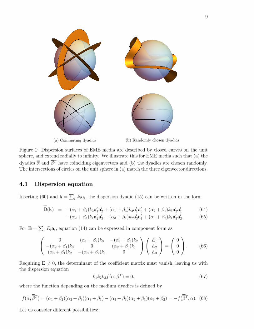
(a) Commuting dyadics (b) Randomly chosen dyadics

Figure 1: Dispersion surfaces of EME media are described by closed curves on the unitsphere, and extend radially to infinity. We illustrate this for EME media such that (a) the

dyadics α and βT have coinciding eigenvectors and (b) the dyadics are chosen randomly.The intersections of circles on the unit sphere in (a) match the three eigenvector directions.

4.1 Dispersion equation

Inserting (60) and k =∑

i kiai, the dispersion dyadic (15) can be written in the form

D(k) = −(α1 + β2)k3a′1a′2 + (α1 + β3)k2a

′1a′3 + (α2 + β1)k3a

′2a′1 (64)

−(α2 + β3)k1a′2a′3 − (α3 + β1)k2a

′3a′1 + (α3 + β2)k1a

′3a′2. (65)

For E =∑

i Eiai, equation (14) can be expressed in component form as 0 (α1 + β2)k3 −(α1 + β3)k2−(α2 + β1)k3 0 (α2 + β3)k1(α3 + β1)k2 −(α3 + β2)k1 0

E1

E2

E3

=

000

. (66)

Requiring E 6= 0, the determinant of the coefficient matrix must vanish, leaving us withthe dispersion equation

k1k2k3f(α, βT ) = 0, (67)

where the function depending on the medium dyadics is defined by

f(α, βT ) = (α1 + β2)(α2 + β3)(α3 + β1)− (α1 + β3)(α2 + β1)(α3 + β2) = −f(βT , α). (68)

Let us consider different possibilities:

10

(a) δ = 10 (b) δ = 1

(c) δ = 0.1 (d) δ = 0

Figure 2: Dispersion surfaces for a magnetoelectric medium defined by (70) and (71). Forδ → 0 the medium becomes an extreme magnetoelectric (EME) medium whose dispersionsurface consists of three orthogonal planes extending to infinity. For finite values of δ,cross sections of the quartic surfaces are shown.

• For the skewon special case with α = βT , we have that f(α, α) = 0, whence (67) isagain identically satisfied for any k.

• For the principal-axion special case with αi = −βi, (67) reduces to the simpler form

k1k2k3(α1 − α2)(α2 − α3)(α3 − α1) = 0. (69)

• When the dyadics α and β are related so that the function f(α, βT ) vanishes, thedispersion equation is satisfied for any k and the medium becomes an example ofan NDE medium. For the principal-axion case (69), this happens when at least twoof the eigenvalues αi coincide.

• For f(α, βT ) 6= 0, the dispersion equation (67) is reduced to k1k2k3 = 0, whenceat least one of the components ki must vanish. This means that any wave vectork 6= 0 must be parallel to one of the three eigenplanes defined by the three pairs ofeigenvectors {ai, aj}, while k = 0 for all directions outside these three eigenplanes.Thus, instead of a well-defined dispersion surface, the possible k vectors specifythree planes intersecting along the three eigenvectors ai, with a common point atthe origin. This is demonstrated in Figure 1a, which presents the dispersion surfaceas truncated by two spherical surfaces. For comparison, in Figure 1b, the resulting

11

dispersion surface is shown for two dyadics α and β created by two randomly chosenmatrices possessing real eigenvectors.

The emergence of the unusual dispersion surface consisting of three planes can be visual-ized by adding permittivity and permeability dyadics to the medium equations as(

DH

)=

(α δεoI

δI/µo β

)·(

BE

), (70)

and letting δ approach zero. If the principal-axion EME medium is defined by the nor-malized symmetric dyadics

ηoβ = −ηoα = u1u1 + 2u2u2 + 4u3u3, (71)

where the normalized eigenvectors ui are orthogonal, the wave vectors are restricted tothe orthogonal eigenplanes ui · r = 0 for i = 1, 2 and 3.

The effect of δ is portrayed in Figure 2, showing cross cuts of the corresponding quarticdispersion surfaces by a plane parallel to one of the eigenplanes. It is seen that, startingfrom a spherical dispersion surface for δ = ∞ (not shown in the figure), for decreasingvalues of δ it is split in two surfaces, one of which shrinks towards the origin (k→ 0), whilethe other approaches the planes corresponding to the three orthogonal eigenplanes. Then,any k vector on the three planes is a valid solution. Dispersion equations for less extrememagnetoelectric media can also yield exotic dispersion surfaces, as has been demonstratedin [28].

The dispersion equation of a generic linear medium has the form D(ω,k) = 0, wherethe left-hand side is a homogeneous quartic polynomial in ω and k. Linear media canbe classified according to how, if at all, D(ω,k) factorizes in homogeneous polynomialsof lower degree. In the general case [13, 25], and in complicated media such as biaxialcrystals [29, 30], no factorization takes place. Media such that D(ω,k) is the product oftwo quadratic polynomials are well studied. Examples include hyperbolic metamaterials[31, 32], uniaxial media [29, 30], nematic liquid crystals [33] and decomposable (DCM)media [34, 35]. If the two quadratic factors coincide, the material displays no birefrin-gence. Isotropic media belong to this class and, to a great extent, summarize its properties[36, 37]. The present article considers two seemingly unexplored factorisations of D(ω,k).For generic EME media, the quartic dispersion polynomial is the product of a linear poly-

nomial, ω, and a cubic irreducible one, detD(k). When α and βT satisfy (59), this latterquantity becomes factorable, see (67). Thereby, EME media with commuting dyadics areexamples of materials such that D(ω,k) is the product of four linear polynomials in ωand k.

4.2 Fields

In an EME medium with commuting dyadics, see (59), the components of the electricfield satisfy the following relations extracted from (66),

(α1 + β2)k3E2 = (α1 + β3)k2E3, (72)

(α2 + β3)k1E3 = (α2 + β1)k3E1, (73)

(α3 + β1)k2E1 = (α3 + β2)k1E2. (74)

12

Equating the product of the left-hand sides with that of the right-hand sides yields thedispersion equation (67), multiplied by E1E2E3.

To understand how the k vector and the field vectors are related, let us assume that the

dyadics α and β obey f(α, βT ) 6= 0, see (68). In this scenario, the dispersion equationrequires that ki = 0 for at least one value of i = 1, 2, 3. Geometrically, the dispersionsurface is made up of three eigenplanes, and wave vectors in all other directions mustvanish, k = 0. Let us examine the case k3 = 0 with k 6= 0, so that (72) and (73) yieldE3 = 0. Similar results are obtained for the other two cases, k1 = 0 and k2 = 0, by achange of indices. To derive the electromagnetic fields, it is convenient to express thewave vector in the relevant eigenplane as

k = k(a1 cosϕ+ a2 sinϕ). (75)

By using (74), the Maxwell equation (12), and the medium law (4) with (60), one thencalculates that

E = a1S(α3 + β2) cosϕ+ a2S(α3 + β1) sinϕ, (76)

ωB = a′3kS(β1 − β2) sinϕ cosϕ, (77)

ωD = a′3kSα3(β1 − β2) sinϕ cosϕ, (78)

H = a1Sβ1(α3 + β2) cosϕ+ a2Sβ2(α3 + β1) sinϕ, (79)

where S is an arbitrary scalar. It is observed that the angle ϕ rotates the fields E and Hin the plane of {a1, a2} while affecting the magnitude of the vectors B and D normal tothat plane. From

E×H = a′3(S2/2)(β1 − β2)(α3 + β2)(α3 + β1) sin(2ϕ), (80)

we can further see that, if ϕ = nπ/2, the vectors E,H and k are parallel to each otherand to either a1 (n even) or a2 (n odd). These cases correspond to waves propagating

along an eigendirection of the dyadics α and β with B = D = 0.

Substituting βi = −αi into (76) – (79) determines the field vectors in principal-axion EMEmedia with commuting dyadics. One must however impose that the three eigenvalues αi

are distinct, otherwise f(α, βT ) vanishes, and the above expressions fail.

For the same reason, (76) – (79) are not valid for pure-skewon EME media with commutingdyadics. In this case, the field vectors are given by (45) – (48) together with the expansionof α in (60).

If α and βT satisfy (59), and have identical eigenvalues, we obtain a pure-axion medium(PEMC). Then, (12) and (13) coincide, which leaves a lot of freedom for the fields [38].

5 Uniaxial EME medium

As an example of EME media with vanishing function f(α, βT ) of (68), let us consider

uniaxial media with symmetric commuting dyadics α and β defined by

α = αtIt + α3u3u3, β = βtIt + β3u3u3, It = u1u1 + u2u2, (81)

13

where the vectors ui make an orthonormal vector basis. Here, ()t denotes componenttransverse to the axial direction u3. In the general case, none of the Hehl–Obukhovcomponents αi defined by (9) – (11) vanish. The number of free parameters for thismedium is reduced to 2(u3) + 4(αt, α3, βt, β3) = 6.

5.1 Plane wave in uniaxial medium

Since the uniaxial EME medium makes another example of an NDE medium, there is noa priori restriction for the choice of the wave vector k. From (14) and (15) we have

u3 · D(k) · E = 0, ⇒ (α3 + βt)kt × Et = 0, (82)

whence, assuming α3+βt 6= 0, the fields transverse to the axial direction can be representedby

Et = U ′kt, Ht = βtU′kt, kt = It · k, (83)

for some factor U ′. Because of

ωu3 ·B = u3 · kt × Et = 0, ωu3 ·D = −u3 · kt ×Ht = 0, (84)

the axial components of B and D vectors actually vanish in the uniaxial EME medium,

u3 ·B = u3 ·D = 0. (85)

Expanding

(k× E− ωB)t = k3u3 × Et − E3u3 × kt − ωBt = 0, (86)

(k×H + ωD)t = k3βtu3 × Et − β3E3u3 × kt + ωαtBt = 0, (87)

inserting (83) and eliminating u3 × kt, we have either kt = 0 and Bt = 0 or

E3 = (αt + βt)k3U, U = U ′/(αt + β3). (88)

Since the first possibility leads to vanishing of all fields in the medium, we can omit thatpossibility. Applying (88), the fields can be constructed as

E = U((αt + β3)kt + (αt + βt)k3u3), (89)

H = U(βt(αt + β3)kt + β3(αt + βt)k3u3) = β · E, (90)

ωB = U(β3 − βt)k3u3 × kt, (91)

ωD = Uαt(β3 − βt)k3u3 × kt = αtωB. (92)

It is remarkable that, in a given uniaxial EME medium, the k vector can be freely chosen,after which the field polarizations are uniquely determined.

14

5.2 Interface of uniaxial EME medium

Assuming continuity of fields through a planar interface n · r = 0 of an isotropic mediumand the uniaxial EME medium defined by (81), the interface conditions for the sum ofthe incident and reflected fields from (89) and (90) become

n× (Ei + Er) = Un× ((αt + β3)kt + (αt + βt)k3u3) (93)

n× (Hi + Hr) = Un× (βt(αt + β3)kt + β3(αt + βt)k3u3) (94)

ωn · (Bi + Br) = U(β3 − βt)k3n · u3 × kt, (95)

ωn · (Di + Dr) = Uαt(β3 − βt)k3n · u3 × kt, (96)

where n denotes the unit vector normal to the interface. In certain cases there may ariseinduced surface sources at the interface to balance the fields on both sides.

As an example, let us consider reflection from a planar interface with normal of theinterface coinciding with the axis of the medium, n = u3. Because of rotational symmetry,we can assume for simplicity that incident and reflected wave vectors are of the form

ki = u1k1 + u3ki3, kr = u1k1 − u3k

i3. (97)

The wave vector tangential to the interface kt = u1k1 6= 0 is shared by the plane wavetransmitted into the EME medium. The conditions for the incident and reflected fields(93), (94), (95) and (96) can be written as

(Ei + Er)t = U(αt + β3)u1k1, (98)

(Hi + Hr)t = Uβt(αt + β3)u1k1, (99)

ωu3 · (Bi + Br) = 0, (100)

ωu3 · (Di + Dr) = 0. (101)

From (100) and (101) it appears that the interface acts as a surface with DB boundaryconditions [18, 39]. However, because of the unknown quantity U in (98) and (99), wemust verify this assumption.

It is known that the DB boundary has eigenfields polarized TE and TM with respect tothe normal direction, and for the eigenfields, the DB boundary is equivalent to PEC andPMC boundaries, respectively [18, 39, 40]. Let us verify this by considering reflection ofincident TE and TM waves from the uniaxial EME interface. The two waves are definedby the conditions

u3 · EiTE = 0, (102)

u3 ·HiTM = 0. (103)

For the TE wave, from (101) we obtain

u3 · ErTE = 0. (104)

Applying the orthogonality conditions

ki · Ei = (u1k1 + u3ki3) · (u1E

iTE1 + u2E

iTE2) = k1E

iTE1 = 0, (105)

15

kr · Er = (u1k1 − u3ki3) · (u1E

rTE1 + u2E

rTE2) = k1E

rTE1 = 0, (106)

we haveEi

TE1 = ErTE1 = 0. (107)

From (98) we obtain

u2 · (EiTE + Er

TE)t = 0, (108)

u1 · (EiTE + Er

TE)t = U(αt + β3)k1 = 0. (109)

The latter yieldsU = 0, (110)

whence the fields in the EME medium must actually vanish. The reflected field satisfies

ErTE = −Ei

TE = −u2EiTE2, (111)

which can be recognized as the PEC boundary condition for the electric field. Expanding

ωµo(HiTE + Hr

TE)t = (ki × EiTE + kr × Er

TE)t

= −u1ki3(E

iTE2 − Er

TE2)

= −2u1ki3E

iTE2 6= 0, (112)

we find that (99) cannot be valid for U = 0. Thus, there must exist an induced surfacecurrent Js, whence (99) must be replaced by [26]

(Hi + Hr)t = Uβt(αt + β3)kt − u3 × Js = −u3 × Js. (113)

The surface current can be found from

Js =1

ωµo

u3 × (−2u1ki3E

iTE2) = − 2ki3

ωµo

u2EiTE2. (114)

(101) must also be upgraded as

ωu3 · (Di + Dr) = kt · Js = − 2ki3ωµo

k1u1 · u2EiTE2 = 0, (115)

but this does not actually change (101). The magnetic fields are found as

HiTE =

1

ωµo

ki × u2EiTE2 =

1

ωµo

(k1u3 − ki3u1)EiTE2 (116)

HrTE =

−1

ωµo

kr × u2EiTE2 = − 1

ωµo

(k1u3 + ki3u1)EiTE2 (117)

whence we can verify the relations

u3 · (BiTE + Br

TE) = ωµou3 · (HiTE + Hr

TE) = 0, (118)

and

(HiTE + Hr

TE)t = − 2ki3ωµo

u1EiTE2 = −u3 × Js. (119)

16

Thus, the interface of the uniaxial EME medium acts as a PEC boundary for the TEplane wave.

For the TM case we can proceed similarly and find that the interface acts as a PMCboundary. Changing symbols, we can rewrite the above results as

U = 0 (120)

andHr

TM = −HiTM = −u2H

iTM2. (121)

In this case we must change the conditions (98) and (100) to

(Ei + Er)t = U(αt + β3)u1k1 + u3 × Jms = u3 × Jms, (122)

ωu3 · (Bi + Br) = −kt · Jms. (123)

The magnetic surface current becomes

Jms = −2ki3ωεo

u2HiTM2, kt · Jms = 0. (124)

and

ErTM =

−1

ωεo(k1u3 + ki3u1)H

iTM2. (125)

To summarize, the interface of the uniaxial EME medium acts as a DB boundary becausethe interface conditions (100) and (101) do not contain surface sources.

6 Conclusion

A novel class of electromagnetic media, labeled as that of extreme magnetoelectric (EME)media, was introduced in terms of two medium dyadics, α, creating electric polarization

through the magnetic field and β, creating magnetic polarization through the electric

field. For the more general bi-anisotropic media, α and β are known as magnetoelectricdyadics, but, in this extreme case, the permittivity and inverse permeability dyadicsare assumed to vanish. Plane wave propagation in EME media was considered withseveral examples of special cases. It was shown that, for a fixed nonzero frequency ω, thedispersion equation corresponding to an EME medium is cubic and homogeneous in thek vector, whence the magnitude of k is not restricted. Actually, the dispersion surface isa conical surface defined by the origin and a closed curve, or a set of closed curves, onthe unit sphere. However, applying 4D formalism (not considered here), one can showthat the dispersion equation is actually quartic with ω = 0 as another possible solution.In many special cases the dispersion equation is reduced to an identity, satisfied for anyk vector, whence the medium is an example of NDE (no dispersion equation) medium.

We demonstrated that, for non-NDE EME media with commuting dyadics α and βT , thedispersion surface is reduced to three intersecting eigenplanes, defined by the three pairsof common eigenvectors of the two dyadics. Wave reflection from an interface of a uniaxialEME medium was considered when the axis of the medium is normal to the interface,in which case the interface was shown to act as a DB boundary with vanishing normalcomponents of the D and B vectors. To extend the present analysis, complex solutionsto the dispersion equation and the corresponding field equations, ignored here, should bestudied.

17

Acknowledgments

The authors thank Professor Friedrich W. Hehl for many comments on the draft of thispaper. A.F. gratefully acknowledges financial support from the Gordon and Betty MooreFoundation.

Appendix 1: Hehl–Obukhov decomposition

The set of medium dyadics of any electromagnetic medium can be most naturally decom-posed in three subsets,(

α ε′

µ−1 β

)=

(α1 ε

′1

µ−11 β1

)+

(α2 ε

′2

µ−12 β2

)+

(α3 ε

′3

µ−13 β3

), (126)

respectively labeled as the principal, skewon and axion parts of the medium by Hehl andObukhov [13]. Such a decomposition can be most logically introduced by applying thefour-dimensional formalism, details of which can be found in [13, 25]. For the 3D Gibbsiandyadic quantities considered here, the decomposition can be defined in somewhat awkwardmanner by reformulating the medium equations (1) and (2) as(

DH

)=

(−ε′ α

−β µ−1

)·(−EB

). (127)

The Hehl–Obukhov decomposition can now be expressed as [13](−ε′ α

−β µ−1

)=

(−ε′1 α1

−β1 µ−11

)+

(−ε′2 α2

−β2 µ−12

)+ α3

(0 I

I 0

), (128)

where the principal part and the skewon part are respectively represented by symmetricand antisymmetric dyadic matrices. However, the symmetric axion part must be extracted

from the first symmetric matrix through the condition trα1 = trβ1 = 0. Thus, thedecomposed medium dyadics satisfy the following relations:

1. Principal part: ε′1 = ε

′T1 , µ−11 = µ−1T1 , α1 = −βT

1 , trα1 = 0;

2. Skewon part: ε′2 = −ε′T2 , µ−12 = −µ−1T2 , α2 = βT

2 ;

3. Axion part: ε′3 = 0, µ−13 = 0, α3 = −β3 = α3I.

References

[1] P. Curie, “Sur la symetrie dans les phenomenes physiques, symetrie d’un champelectrique et d’un champ magnetique”, Journal de Physique, 3rd Series, Vol. 3, pp.393–415, 1894.

18

[2] P. Debye,“Bemerkung zu einigen neuen Versuchen uber einen magneto-elektrischenRichteffekt”, Zeitschrift fur Physik, Vol. 36, pp. 300–301, 1926.

[3] L.D. Landau and E.M. Lifshitz, Electrodynamics of Continuous Media, Oxford: Perg-amon Press, 1960.

[4] D.N. Astrov, “The magnetoelectric effect in antiferromagnetics,” Sov. Phys. JETP,Vol.11, No. 3, pp. 708–709, 1960.

[5] T.H. O’Dell, The Electrodynamics of Magneto-Electric Media, Vol. XI, Selected Top-ics in Solid State Physics. Amsterdam: North-Holland Publ. Co., 1970.

[6] A. D. Yaghjian, “Extreme electromagnetic boundary conditions”, Metamaterials,Vol. 4, Nos. 2-3, pp. 70–76, 2010.

[7] A. Sihvola, H. Wallen, P. Yla-Oijala and J. Markkanen, “Material realizations ofextreme electromagnetic boundary conditions and metasurfaces,” XXX URSI GASS,Istanbul Aug. 2011, (4 pages).

[8] A. Alu and N. Engheta, “Extremely anisotropic boundary conditions and their opticalapplications,” Radio Sci., Vol. 46, No. 5, Oct. 2011 (8 pages).

[9] Y. Radi and S. A. Tretyakov, “Electromagnetic phenomena in omega nihility media,”Metamaterials 2012, St Petersburg, June 2012, pp.764–766.

[10] A.V. Kildishev, A. Boltasseva and V.M. Shalaev, “Planar photonics with metasur-faces,” Science, Vol. 339, 1232009, 2013.

[11] N. Yu and F. Capasso, “Flat optics with designer metasurfaces,” Nature Materials,Vol. 13, pp. 139-150, 2014.

[12] I.V. Lindell and A.H. Sihvola, “Perfect electromagnetic conductor”, J. Electro. WavesAppl., Vol. 19, No. 7, pp. 861-869, 2005.

[13] F.W. Hehl and Y.N. Obukhov, Foundations of Classical Electrodynamics, Boston:Birkhauser, 2003.

[14] F.W. Hehl, Yu.N. Obukhov, J.-P. Rivera, and H. Schmid, “Relativistic nature of amagnetoelectric modulus of Cr2O3 crystals: A four-dimensional pseudoscalar and itsmeasurement,” Phys. Rev. A 77, 022106, February 2008,

[15] Shahvarpour, A., T. Kodera, A. Parsa and C. Caloz, “Arbitrary electromagneticconductor boundaries using Faraday rotation in a grounded ferrite slab” IEEE Trans.Microwave Theory Tech., Vol. 58, No. 11, pp. 2781–2793, 2010.

[16] El-Maghrabi, H. M., A. M. Attiya and E. A. Hashish, “Design of a perfect electro-magnetic conductor (PEMC) boundary by using periodic patches,” Prog. Electromag.Res. M, Vol. 16, pp. 159–169, 2011.

[17] I.V. Lindell and A. Sihvola, “Simple skewon medium realization of DB boundarycondition,” Prog. Electromag. Res. Letters, Vol. 30, pp. 29–39, 2012.

19

[18] Lindell, I. V. and A. Sihvola, “Electromagnetic boundary condition and its realizationwith anisotropic metamaterial,” Phys. Rev. E, Vol. 79, No. 2, 026604 (7 pages), 2009.

[19] A. Sihvola, H. Wallen, P. Yla-Oijala, M. Taskinen, H. Kettunen and I.V. Lindell,“Scattering by DB spheres,” IEEE Antennas Wireless Propag. Lett., Vol. 8, pp. 542-545, 2009.

[20] I.V. Lindell, A. Sihvola, P. Yla-Oijala and H. Wallen, “Zero backscattering fromself-dual objects of finite size,” IEEE Trans. Antennas Propag., Vol. 57, No. 9, pp.2725-2731, 2009.

[21] Zhang, B., H. Chen, B.-I. Wu and J. A. Kong, “Extraordinary surface voltage effectin the invisibility cloak with an active device inside,” Phys. Rev. Lett., Vol. 100,063904, 2008.

[22] Yaghjian, A. and S. Maci “Alternative derivation of electromagnetic cloaks and con-centrators,” New J. Phys., Vol. 10, 115022, 2008; “Corrigendum”, ibid, Vol. 11,039802, 2009.

[23] Zaluski, D., D. Muha and S. Hrabar, “DB boundary based on resonant metamaterialinclusions,” Metamaterials’2011, Barcelona, October, pp. 820–822, 2011.

[24] Zaluski, D., S. Hrabar and D. Muha, “Practical realization of DB metasurface,” Appl.Phys. Lett., Vol. 104, 234106, 2014.

[25] I.V. Lindell, Multiforms, Dyadics and Electromagnetic Media, Hoboken, N.J.: Wileyand IEEE Press, 2015.

[26] I.V. Lindell, Methods for Electromagnetic Field Analysis, 2nd ed., Oxford: UniversityPress, 1995.

[27] Lindell, I. V. and A. Favaro, “Electromagnetic media with no dispersion equation,”Prog. Electro. Res B, Vol. 51, pp. 269–289, 2013.

[28] A. Favaro and F. W. Hehl, “Light propagation in local and linear media: Fresnel-Kummer wave surfaces with 16 singular points”, Phys. Rev. A 93, 013844, 2016.

[29] F.A. Jenkins and H.E. White, Fundamentals of Optics, 3rd ed., New York, NY:McGraw-Hill, 1957.

[30] M. Born and E. Wolf, Principles of Optics, 7th expanded ed., Cambridge, UK: Uni-versity Press, 1999.

[31] A. Poddubny, I. Iorsh, P. Belov and Y. Kivshar, “Hyperbolic metamaterials,” NaturePhotonics, Vol. 7, pp. 958-967, 2013.

[32] L. Ferrari, C. Wu, D. Lepage, X. Zhang and Z. Liu, “Hyperbolic metamaterials andtheir applications,” Prog. Quantum Electron., Vol. 40, pp. 1-40, 2015.

[33] Y.N. Obukhov, T. Ramos and G.F. Rubilar, “Relativistic Lagrangian model of anematic liquid crystal interacting with an electromagnetic field,” Phys. Rev. E, Vol.86, 031703, 2012.

20

[34] I.V. Lindell, L. Bergamin and A. Favaro, “Decomposable medium conditions in four-dimensional representation,” IEEE Trans. Antennas Propagat., Vol. 60, No. 1, 2012.

[35] M.F. Dahl, “Characterisation and representation of non-dissipative electromagneticmedium with two Lorentz null cones,” J. Math. Phys., Vol. 54, 011501, 2013.

[36] A. Favaro and L. Bergamin, “The non-birefringent limit of all linear, skewonlessmedia and its unique light-cone structure,” Ann. Phys. (Berlin), Vol.523, No. 5,pp.383-401, 2011.

[37] M.F. Dahl, “Determination of an electromagnetic medium from the Fresnel surface,”J. Phys. A: Math. Theor., Vol. 45, 405203, 2012.

[38] B. Jancewicz, “Plane electromagnetic wave in PEMC”, J. Electro. Waves Appl.,Vol.20, No. 12, pp.647–659, 2006.

[39] I.V. Lindell and A. Sihvola, “Uniaxial IB-medium interface and novel boundary con-ditions,” IEEE Trans. Antennas Propagat., Vol. 57, No. 3, pp. 694–700, March 2009.

[40] I.V. Lindell and A. Sihvola, “Electromagnetic boundary conditions defined in termsof normal field components,” IEEE Trans. Antennas Propag., Vol. 58, No. 4, pp.1128–1135, April 2010.