planned sampling of spatially varying brdfsmjh7v/bib/lensch03a.pdfpublishers, 108 cowley road,...

EUROGRAPHICS 2003 / P. Brunet and D. Fellner(Guest Editors)

Volume 22 (2003), Number 3

Planned Sampling of Spatially Varying BRDFs

Hendrik P.A. Lensch1, Jochen Lang1, Asla M. Sá2 †, and Hans-Peter Seidel1

1 MPI Informatik, Saarbrücken, Germany2 Instituto Nacional de Matemática Pura e Aplicada - IMPA, Brazil

AbstractMeasuring reflection properties of a 3D object involves capturing images for numerous viewing and lightingdirections. We present a method to select advantageous measurement directions based on analyzing the estimationof the bi-directional reflectance distribution function (BRDF). The selected directions minimize the uncertaintyin the estimated parameters of the BRDF. As a result, few measurements suffice to produce models that describethe reflectance behavior well. Moreover, the uncertainty measure can be computed fast on modern graphics cardsby exploiting their capability to render into a floating-point frame buffer. This forms the basis of an acquisitionplanner capable of guiding experts and non-experts alike through the BRDF acquisition process. We demonstratethat spatially varying reflection properties can be captured more efficiently for real-world applications using ouracquisition planner.

Categories and Subject Descriptors (according to ACM CCS): I.3.7 [Computer Graphics]: Three-DimensionalGraphics and Realism Virtual Reality I.4.1 [Computer Vision]: Digitization and Image Capture, Reflectance

1. Introduction

In the field of 3D object acquisition progress has been madeboth in the area of geometry and appearance acquisition.Appearance or reflection properties are in most approachesmeasured by capturing a number of samples of the BRDFof the object. The samples are commonly acquired by a sen-sor (a digital camera in our set-up) and a point-light source.One pair of light source and camera position (called a viewcollectively in the remainder of this paper) captures a singlereflectance sample for each point that is visible and lit.

A number of researchers have built special gantries toperform a robot controlled dense sampling of the reflectionproperties 8, 28, 10, 30. Others position the camera and the lightsource manually 23, 25, 19, 20.

The basic question for both, the automatic and the man-ual approach is: How to sample the reflection properties inan efficient way? The acquisition of reflection propertiesneeds to be planned in order to measure efficiently, failingto plan may result in insufficient data for the modeling taskor lead to highly redundant over-sampling. Measurement is

† This work was conducted at MPI Informatik.

Figure 1: Comparison of Spatially Varying BRDF Models.The model 19 on the left contains holes in the BRDF due toundersampling. The model on the right obtained from thesame number of views suggested by our planner samples thesurface evenly.

typically an involving task and efficiency in the process is ofparamount importance.

In this paper we present a method that assesses the uncer-tainty in the parameters of a Lafortune model 16 (The under-lying method is however also applicable to other paramet-ric models and may be adapted to non-parametric modelsas well.) Based on this uncertainty measure we develop anacquisition planning algorithm that computes from where to

c© The Eurographics Association and Blackwell Publishers 2003. Published by BlackwellPublishers, 108 Cowley Road, Oxford OX4 1JF, UK and 350 Main Street, Malden, MA02148, USA.

Lensch et al. / Planned Sampling of Spatially Varying BRDFs

sample next in order to minimize the uncertainty in the pa-rameters, i.e., where to place the camera and the light sourcewith respect to a set of previously acquired views. For 3Dobjects we have to evaluate and combine the predicted un-certainty of each single surface point. A good set of viewswill measure each point on the surface several times withvaried viewing and lighting directions sampling a highlightat each point. The view planning is influenced by a num-ber of further constraints including the 3D shape. The shapelimits the number of visible and lit surface points in a view.

One of the goals of acquisition planning is to performmeasurements efficiently. Time spent on the planning itselftherefore has to be reasonable. We compute the uncertaintymeasure in modern graphics hardware with floating-pointframe buffers. The evaluation is performed directly on thetexture atlas of the object.

The measurement theory behind our approach is well es-tablished in other fields; physicists and other natural sci-entists apply it quite routinely to their measurement tasks.Our contribution in this area is to adapt some of the naturalsciences’ measurement theory to the task of measuring theBRDF for computer graphics. Our paper makes three maincontributions:

• the definition of a function to measure the reduction inuncertainty added by one view (camera and light sourceposition),

• a view planning algorithm that combines this functionwith geometric constraints imposed by a 3D object to pre-dict the next best view for efficient measurement, and

• a hardware-accelerated implementation for evaluation ofthe objective function directly on the texture atlas.

In the next section we discuss related work before wepresent an overview over the acquisition planning and themeasurement process in Section 3.

2. Related Work

Work related to the automated acquisition of reflection prop-erties of complete objects can be found in different fieldsincluding computer graphics, computer vision, robotics andvisual metrology. We start our review with a brief summaryof work in computer vision, followed by a discussion of au-tomatic scanning of 3D models including some theoreticalissues, and we conclude our review with work on BRDF ac-quisition and representation in computer graphics.

The task of exploring unknown spatially-varying BRDFof an object relates directly to viewpoint control in computervision, e.g., in minimizing uncertainty of 3D object repre-sentations 45 and in scene exploration 15 Related to BRDFacquisition are also visual metrology tasks which are re-viewed by Tarabanis and Tsai 42. In metrology the planningtask is to position a sensor to satisfy some sensing qualitycriterion, e.g., work by Cowan and Kovesi 6 and Mason and

Grün 26. The quality criterion of interest in our work is thecertainty in the acquired BRDF. We aim at achieving highquality by choosing advantageous viewpoints of camera andlight source positions.

The placement of a camera relative to an object has beenplanned for geometric model acquisition with a robotic fa-cility 36, 17 and with an automated commercial scanner 33. Inpractice, view planning is often started after an initial roughacquisition of the object’s geometry from pre-set viewpoints,as in the geometry model acquisition system by Reed andAllen 36, 37. The task in this situation is to fill holes in theexisting model stemming from tight visibility restrictions.Filling holes is an example where an automated planner canbe very beneficial.

The incremental Next Best View planning strategy ofWhaite and Ferrie 45 is closely related to ours. Their strategyexplores the geometry of a 3-D model with a priori unknownshape. They apply a synthesis approach which is based on aprobabilistic model of an object’s geometry to be explored.The approach minimizes uncertainty of a parametric objectmodel. Objects are represented by sets of superquadrics. Us-ing an active sensing strategy a next view is selected. The se-lected view minimizes the current uncertainty of the objectmodel. The algorithm is applied to explore the environmentof a robotic agent enabling object recognition and manipu-lation.

An alternative approach to view planning is to delegatethe (computationally complex) task to a human but to pro-vide real-time feedback. This has been demonstrated suc-cessfully by Rusinkiewicz et al. 38 for geometry scanning ofobjects. Planning the acquisition of reflectance properties inthis fashion is however impossible since humans can gen-erally not reason about the four-dimensional BRDF on thesurface of complex objects in real-time.

In computational geometry, visibility in polygonal envi-ronment is considered 5 with applications in geographicaldata processing, security and military 22. Acquiring realis-tic reflectance properties of a 3D object requires imaging itscomplete surface. This completeness constraint restricts theset of possible solutions in acquisition planning. Finding theminimal set of views which cover the complete surface of anobject is a NP-hard problem 43. A planned set of views maystill fail in practice due to positioning or modeling errors andoff-line plans need to consider uncertainty to ensure cover-age of the complete surface when actually executed 43, 40.

In computer graphics, the imaging of visible surfaces isrelevant in radiosity, ray-tracing, scene walk-throughs andtexturing of surfaces 41 as well as for image-based render-ing 13, 4, 44. In the BRDF measurement and representationfield, quite a number of articles have been published but,to the best of our knowledge, so far only Kay and Caelli 14

have investigated the dependency between measurement andthe qualtiy of the estimated BRDF. McAllister 30 computes

c© The Eurographics Association and Blackwell Publishers 2003.

474


ClusteringRegistration ResampleShadow/Visibility

BRDFFittingPlanning Acquisition

ViewView

Figure 2: View planning interacts with the entire pipeline of appearance measurements: An optimal view is proposed andcaptured. Manual placement of camera and light source requires registration with the 3D object. Visibility and shadows arecomputed and the data is resampled. From the resampled data of all views the BRDF parameters per cluster are updated whichagain influence the planning of the next view.

the number of samples required to densely cover the hemi-sphere above a point with a light source. Ramamoorthi andHanrahan 35 examine the problem of global inverse illumina-tion within a signal processing framework. Existing BRDFmeasurement approaches can be classified by the number ofimages necessary and the generality of the estimated BRDFmodel.

A family of methods measure reflectance properties byperforming a very dense sampling. Some of them are de-signed for flat surface samples only 7, 30 while others candeal with 3D objects 8, 27, 28, 29, 10. Since a dense sampling al-lows to render directly from the measured data, the reflectionproperties are unrestricted in those approaches. The qualityof the outcome when no BRDF model is fit mainly dependson the sampling density.

A variety of techniques estimate the appearance of an ob-ject from a sparse set of images. In many of these approachesthe specular part of the BRDF is restricted to be constantover a small patch or even over the entire object. Measure-ments in these approaches are typically performed either byusing a point light source 39, 25, 24, 31, 19, 20, 21 or by perform-ing inverse global illumination 46, 11, 1, 35, 32. Lensch et al. 19, 20

and Li et al. 21 demonstrated how to estimate a varying spec-ular part from a sparse set of views. In both approaches clus-tering techniques are applied to the BRDF parameters overthe object’s surface. In this paper, we also follow a sparsesampling approach but at the same time assuring the qualityof the model. The fully spatially varying model in our workis identical to the one employed by Lensch et al. 20.

Next, we introduce our method which is able to select asparse set of measurements and ensures the quality of theBRDF model at the same time.

3. Acquisition Loop

The measurement of reflection properties is executed as anumber of successive steps which are shown in Figure 2.Prior to the acquisition of reflectance properties the 3D ge-ometry of the object has to be acquired. The acquisitionstarts with the planning of the first view. Each new view isplanned based on the current estimate of the BRDF parame-ters and the visibility and shadowing constraints imposed bythe 3D geometry of the object.

In the second step the planned view is acquired. Next, the

view is registered with the 3D object 18, since the real cam-era and light source position may deviate from the proposedview. The recovered positions are used to determine the re-gions of the object’s surface which are visible and lit. Thevalid pixels are resampled into a texture atlas.

For the planning a coarse texture atlas is used to speed upthe process. Local viewing and lighting direction are com-puted per pixel. From the resampled data a new set of BRDFparameters is estimated. As the number of measurements fora single point are too few to obtain credible BRDF parame-ters, clusters of points are used to fit the parameters. Pointscan be clustered either based on their diffuse color or usingthe method by Lensch et al. 20. The estimated spatially vary-ing BRDF parameters are then used in the next execution ofthe planning step.

After the capturing process is complete, all measurementdata is resampled again using a high resolution texture atlasand a final spatially varying reflection model is estimated.

Planning is performed by minimization of an objectivefunction that takes into account the previously acquired data,the geometry of the object and the currently estimated BRDFparameters. The objective function is based on co-variancematrices as an uncertainty measure. The co-variance matri-ces are compact and summarize all necessary informationabout the views acquired so far. Their storage cost and thecomputation time of planning algorithm is constant and in-dependent of the number of acquired views. In particular, wedo not have to store each local viewing and lighting directionper pixel for each measurement.

In the next section we detail the relationship between theco-variance matrix and measurement uncertainty with an ob-ject consisting of a single pixel as a tutorial example.

4. One-Pixel Objects

Measuring the BRDF of a single point on an object is al-ready a task which involves some effort. It is necessary tounderstand how measurements of the reflectance of a sin-gle pixel influence the reliability of parameters of the BRDFmodel we are going to fit. We briefly summarize backgroundmaterial on parameter estimation and measurement theoryrelated to our fitting approach. We conclude that not all pos-sible measurements contribute in the same way to the qualityof the fitted model parameters.


475


For the purpose of the discussion in this and the next sec-tion, the prior information I for our measurement task is thatwe would like to estimate a Lafortune model fr with oneisotropic specular lobe (see Equation 1) for an object con-sisting of one-pixel.

fr(β;ω) = ρd +(cxωix ωox + cyωiy ωoy + czωiz ωoz)N (1)

where ρd denotes the diffuse reflectance, N the exponent ofthe specular lobe, cx, cy and cz the weighting coefficients ofthe dot product between ωi and ωo; ωi is the incident lightdirection and ωo the exitant lighting direction. In the follow-ing, we denote these parameters collectively as β. The modelM(β,ω) calculates the reflectance for a given ωi and ωo (col-lectively ω). Equation 2 shows the standard regression prob-lem for m measurements with an additive error term ε re-sulting in m reflectance samples Rm. For the purpose of thisdiscussion, we assume that the error terms are independentand identically distributed (iid) samples from a distributioncentered at 0.

Rm = M(β,ωm)+ εm (2)

A principled approach to solve this model fitting task is byemploying Bayes theorem

P(M|DI) =P(M|I)P(D|M)

P(D|I).

Bayes theorem describes how to obtain the posterior prob-ability distribution of the reflectance model P(M|DI). Itdepends on our prior belief of possible model parametersP(M|I), the measurement or predictive probability of a mea-surement P(D|I) with acquired data D and our model ofthe measurement process P(D|M) which here is Equation 2.Measurements are a principled way to change one’s priorbeliefs. If the observations provide strong evidence, the dataterm dominates while with a lack of evidence the prior re-mains unchanged. The certainty in the model is describedby the full distribution P(M|I). The distribution is in the di-mensions of the model and requires a summary for interpre-tation. The most probable parameter value and confidenceintervals are common summaries. (See, e.g., Bretthorst 2 orHastie et al. 12 for a more complete introduction to Bayesianmodel estimation).

An approach to find the most probable model is minimiza-tion. The sum of squared errors

Q = ∑m

(Rm −M(β,ωm))2 (3)

is the most common error measure to minimize. This er-ror measure coincides with the most probable model in theBayesian approach given the model is linear in the parame-ters β, the noise ε in the measurements is Gaussian and ourprior beliefs are uninformative (flat priors) 12. Under thesecircumstances, the uncertainty in the most probable modelparameters depend linearly on the co-variance matrix CoV.The co-variance matrix CoV is the inverse of the Hessianmatrix H with entries Hi, j = ∂2Q

∂βi∂β j(see Appendix A for the

derivatives). The singular values σ of the co-variance matrixdefine the length of the major axes of the hyperellipsoid ofa given Q. In linear models this hypervolume bounded bythe hyperellipsoid for a given quadratic error measure Q isdirectly related to the posterior probability.

In the non-linear Lafortune reflectance model the simplerelationship between the least-squares residual Q and the un-certainty in the parameters does not hold. The most popularway to proceed is to employ a non-linear least-square solverto minimize Q but analyze the fit with the co-variance ma-trix CoV. The co-variance matrix is only strictly valid forlinear models, however, employing CoV is justifiable if Q iswell approximated by a quadratic near the minimum 34. Weperformed some Monte-Carlo bootstrap analysis 9, 3 in orderto confirm the validity of the linear approximation when fit-ting the non-linear Lafortune model. We do not report thedetails here but in summary, our conclusion is that the non-linearity of the Lafortune reflectance model prevents us fromstating confidence intervals based on the linear approxima-tion. However, the co-variance matrix is a good indicator ofparameter uncertainty and if we would like to obtain mea-surements in a way such that we are most confident in theestimated parameters, minimizing the co-variance matrix isa sensible strategy. This conclusion is also consistent withthe reasoning of Whaite and Ferrie 45. The co-variance ma-trix of the Lafortune model depends only on the chosen in-cident and exitant light direction given a fixed estimate β̂. Arecipe of how to choose the light and viewing directions forthe one-pixel object is described in the next section.

5. Uncertainty Minimization

The uncertainty in the estimated parameters for a set ofviews is minimum if the co-variance matrix is minimal. Ifwe are exploring unknown reflectance properties, we onlylearn our model parameters as we acquire new views, gain-ing information incrementally. The certainty gain of a viewis therefore the reduction in the co-variance matrix from theprevious view to the current one and hence, the objectivefunction

F = ‖CoV(β̂v,ω1,...,v)‖−‖CoV(β̂v,ω1,...,v+1)‖. (4)

We would like to maximize the certainty gain, i.e., we haveto maximize F . A greedy strategy selects after each view vthe one which maximizes the expected gain of the next viewv + 1. This greedy strategy is optimal in the linear case withfixed estimates β̂ because then the co-variance is indepen-dent of the order of views. In our scenario this approximationbecomes more appropriate as the certainty in the estimatesincreases.

The selection strategy must also deal with a rank-degenerate Hessian matrix H during the views v = 1 . . .L,where L is the number of parameters in the Lafortune modelfr, in our case L = 4. These initial views have to be chosenin order to arrive at a small ||CoV|| after view v = L. While


476


||CoV|| = ∞ for v < L, we can calculate the Pseudo-Inverseof the Hessian matrix instead. Figure 3(a) shows the singu-lar values σk of the pseudo-inverse which approximately in-crease exponentially with k. We maximize the informationgain based on this pseudo co-variance until the Hessian ma-trix reaches full rank. The gain can be considered infinitewith each rank gained, i.e, a choice of F(k ≤ L) = In f −σksuggests itself. We illustrate this strategy in Figure 3 forthe one-pixel object. (We pick In f = 109 and the parame-ters β = (ρd = 0.3,Ns = 10,cx = cy = −0.8,cz = 0.8) forthe Lafortune model (Equation 1)). A better continuation ofthe objective function towards the first view can be obtainedwith F(k ≤ L) = 10L−k ∗ (In f −σk) which is shown in Fig-ure 3(b). The difference in the two considered choices is onlyof importance in multi-pixel objects when the informationgain at one pixel has to be compared to the information gainat another pixel. Under these circumstances, the exponen-tially increasing function will strongly favour low rank up-dates over high rank updates.

2 4 6 8

100

102

104

106

# Views

log(

σ k)

k=1

k=2

k=3

k=4

(a) σk of CoV

2 4 6 8

105

1010

Views

log(

F)

(b) Obj. Function F

Figure 3: Objective Function F for Infinite Co-Variance.The singular values σk of the CoV show an exponential in-crease with k. Figure 3(b) shows two choices for F whenk ≤ L: F(k ≤ L) = 10L−k ∗ (In f − σk) in red and F(k ≤L) = In f −σk (In f = 109) in blue.

5.1. Maximization

The task of view planning is to maximize the objective func-tion F in Equation 4. Our observation is that the objectivefunction is partially smooth depending on the visibility of agiven view. Globally, it can have many discontinuities dueto shadows and visibility. In order to maximize the objectivefunction we apply a two-step procedure with randomization:

• Search for the best pair of initial positions of camera andlight source on a discretized sphere. Randomize the ori-entation of the discretization before each new view.

• Use a local continuous optimizer to improve the discretesolution found.

The random rotation of the sphere discretization improvesthe discrete search, eventually evaluating all views. This pro-cedure allows us to use a coarse discretization in the discrete

search achieving acceptable coverage at least over multipleviews.

We have tested two downhill non-gradient-based optimiz-ers: the Simplex method and Powell’s method with non-gradient based linear search 34. The Simplex method is ini-tialized with the starting value of the discrete search plus ran-dom points within its neighborhood. Although both methodsmay converge to local maxima, we still achieve good resultsdue to the discrete initialization. In Figure 4, we show thenorm of the co-variance matrix achieved by maximizing Fin Equation 4 with both, the Simplex and Powell’s method.We have observed that Powell’s method requires typicallyless function evaluations but achieves slightly worse resultsthan the Simplex method. Figure 4 also compare the behav-ior of the optimization with the 2−norm ||CoV||2 versusthe Frobenius norm ||CoV||Frob. The difference is negligi-ble due to the exponential rate of decay in the size of thesingular values of the co-variance matrix. Besides planning

10 20 30 4010

4

106

108

# Views

log(

||CoV

|| 2,F

rob)

10 20 30 400.5

1

1.5

2

2.5

3

3.5

4x 104

# Views

||CoV

|| 2,F

rob

Figure 4: Norm of the Co-Variance Matrix during Optimiza-tion. Green ||CoV||2 and red ||CoV||Frob are obtained withPowell’s method, while blue ||CoV||2 and cyan ||CoV||Frobare obtained by the simplex method. The optimization is ap-plied to the one-pixel object.

the next best view, the objective function can be employedto determine when to stop acquiring more views. Observethat the norm decays roughly exponentially as the numberof samples of the one-pixel object increases. It indicates thatone can stop the optimization after the gain in confidence isbelow a pre-defined threshold.

6. Multi-Pixel Objects

We are now generalizing our insights from the one-pixel ob-ject to 3D objects. The reflectance of real-world 3D objectscannot be modeled with sufficient accuracy by a single point.The complete surface area of a 3D object is not visible fromany single given camera and light source position. Thus, thegeometric shape influences the objective function and playsan important role in the uncertainty minimization.

6.1. Homogeneous vs. Spatially Varying BRDFs

Calculation of model uncertainty for a real 3D object re-quires the computation of the the Hessian matrices Hi con-sidering all previous measurements at each point i on the


477


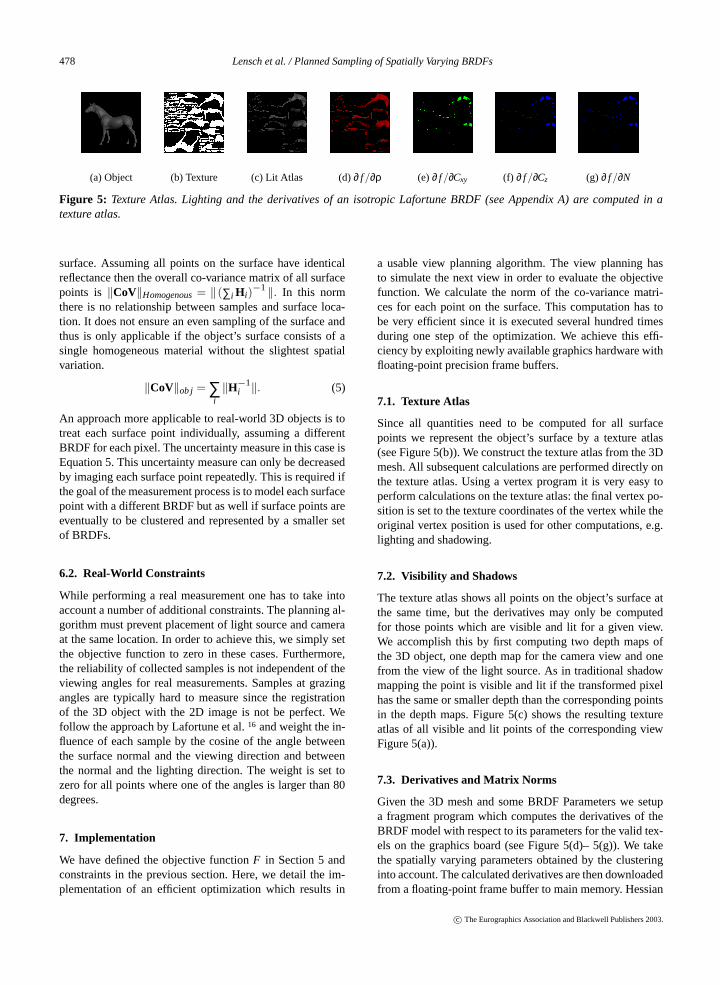
(a) Object (b) Texture (c) Lit Atlas (d) ∂ f/∂ρ (e) ∂ f/∂Cxy (f) ∂ f/∂Cz (g) ∂ f/∂N

Figure 5: Texture Atlas. Lighting and the derivatives of an isotropic Lafortune BRDF (see Appendix A) are computed in atexture atlas.

surface. Assuming all points on the surface have identicalreflectance then the overall co-variance matrix of all surfacepoints is ‖CoV‖Homogenous = ‖(∑i Hi)

−1 ‖. In this normthere is no relationship between samples and surface loca-tion. It does not ensure an even sampling of the surface andthus is only applicable if the object’s surface consists of asingle homogeneous material without the slightest spatialvariation.

‖CoV‖ob j = ∑i‖H−1

i ‖. (5)

An approach more applicable to real-world 3D objects is totreat each surface point individually, assuming a differentBRDF for each pixel. The uncertainty measure in this case isEquation 5. This uncertainty measure can only be decreasedby imaging each surface point repeatedly. This is required ifthe goal of the measurement process is to model each surfacepoint with a different BRDF but as well if surface points areeventually to be clustered and represented by a smaller setof BRDFs.

6.2. Real-World Constraints

While performing a real measurement one has to take intoaccount a number of additional constraints. The planning al-gorithm must prevent placement of light source and cameraat the same location. In order to achieve this, we simply setthe objective function to zero in these cases. Furthermore,the reliability of collected samples is not independent of theviewing angles for real measurements. Samples at grazingangles are typically hard to measure since the registrationof the 3D object with the 2D image is not be perfect. Wefollow the approach by Lafortune et al. 16 and weight the in-fluence of each sample by the cosine of the angle betweenthe surface normal and the viewing direction and betweenthe normal and the lighting direction. The weight is set tozero for all points where one of the angles is larger than 80degrees.

7. Implementation

We have defined the objective function F in Section 5 andconstraints in the previous section. Here, we detail the im-plementation of an efficient optimization which results in

a usable view planning algorithm. The view planning hasto simulate the next view in order to evaluate the objectivefunction. We calculate the norm of the co-variance matri-ces for each point on the surface. This computation has tobe very efficient since it is executed several hundred timesduring one step of the optimization. We achieve this effi-ciency by exploiting newly available graphics hardware withfloating-point precision frame buffers.

7.1. Texture Atlas

Since all quantities need to be computed for all surfacepoints we represent the object’s surface by a texture atlas(see Figure 5(b)). We construct the texture atlas from the 3Dmesh. All subsequent calculations are performed directly onthe texture atlas. Using a vertex program it is very easy toperform calculations on the texture atlas: the final vertex po-sition is set to the texture coordinates of the vertex while theoriginal vertex position is used for other computations, e.g.lighting and shadowing.

7.2. Visibility and Shadows

The texture atlas shows all points on the object’s surface atthe same time, but the derivatives may only be computedfor those points which are visible and lit for a given view.We accomplish this by first computing two depth maps ofthe 3D object, one depth map for the camera view and onefrom the view of the light source. As in traditional shadowmapping the point is visible and lit if the transformed pixelhas the same or smaller depth than the corresponding pointsin the depth maps. Figure 5(c) shows the resulting textureatlas of all visible and lit points of the corresponding viewFigure 5(a)).

7.3. Derivatives and Matrix Norms

Given the 3D mesh and some BRDF Parameters we setupa fragment program which computes the derivatives of theBRDF model with respect to its parameters for the valid tex-els on the graphics board (see Figure 5(d)– 5(g)). We takethe spatially varying parameters obtained by the clusteringinto account. The calculated derivatives are then downloadedfrom a floating-point frame buffer to main memory. Hessian


478


Figure 6: Comparison of Planner and Human Expert. First and third rows show results with the planner, while results obtainedby the human expert are shown in the second and forth row. (Images shown are after every 3rd view.) Notice how the plannerselects samples to cover the object’s surface evenly. The human expert acquires redundant samples of some surface areas (front)while other areas remain undersampled (back and bottom). The images show log(‖CoV‖) color-coded in matlab jet style. Bluemeans high confidence in the estimated BRDF parameters while the uncertainty increases towards red. Black regions have notbeen updated to full rank so far.

matrices for the current view are calculated and added to theaccumulated Hessian matrices of previous views. The resultis inverted using singular value decomposition to obtain thenorms of the co-variance matrices. The final value of the ob-

Task ∂ f/∂β Download H SVD Total

Time[s]

0.119 0.477 0.021 0.523 1.138

Table 1: Time consumed for computing the derivatives, todownload the results to main memory, to add to the Hessianmatrices and to perform the remaining calculations (SVD)in software in order to evaluate the objective function of oneview on a 512x512 texture atlas. Note that on average onlyone fourth of the 147444 valid pixels were visible and lit.

jective function is then computed as the sum of the objectivefunctions of each pixel. All software computations are doneonly at those pixels in the texture atlas which are visible andlit. A total of approximately 440 evaluations of the objectivefunction are performed in the optimization of one view.

Table 7.3 lists how much time is spend for each of thecomputation steps. A considerable amount of time is un-fortunately consumed by downloading the frame buffer. Tosave bandwidth we currently use a monochromatic isotropicLafortune BRDF model with one lobe (4 parameters) for the

view planning. The method can however be easily extendedto work with more complex or multi-lobe models.

8. Measurement Results

We compare the views selected by our method to the viewsselected by a human expert prior to our method. The 3D ob-ject for which the spatially varying BRDF is acquired, arethe angels shown in Figure 1. The reflectance model of the

Rank # Pixels # Pixels σ̄L−k+1 σ̄L−k+1

k Planner Expert Planner Expert

0 10 857 - -1 300 2013 0.06587 0.044822 1755 973 2.3804 0.98233 1412 583 39.170 75.0754 5767 4818 745.16 2308.94

Table 2: Comparison of ‖CoV‖ Obtained by Planner andHuman Expert after 27 views. Shown are the singular valuesaveraged over all pixels. The planner acquired more pixelwith higher rank and higher confidence. (Note the consider-ably smaller singular value in the last row).

angels has previously been captured with a set of 27 views(not shown). Figure 9 shows the images acquired with ourplanner. The planner selects camera and light source posi-tion in order to collect samples of each surface point under


479


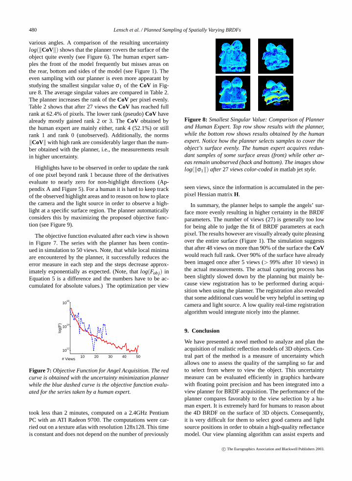
various angles. A comparison of the resulting uncertaintylog(‖CoV‖) shows that the planner covers the surface of theobject quite evenly (see Figure 6). The human expert sam-ples the front of the model frequently but misses areas onthe rear, bottom and sides of the model (see Figure 1). Theeven sampling with our planner is even more appearant bystudying the smallest singular value σ1 of the CoV in Fig-ure 8. The average singular values are compared in Table 2.The planner increases the rank of the CoV per pixel evenly.Table 2 shows that after 27 views the CoV has reached fullrank at 62.4% of pixels. The lower rank (pseudo) CoV havealready mostly gained rank 2 or 3. The CoV obtained bythe human expert are mainly either, rank 4 (52.1%) or stillrank 1 and rank 0 (unobserved). Additionally, the norms‖CoV‖ with high rank are considerably larger than the num-ber obtained with the planner, i.e., the measurements resultin higher uncertainty.

Highlights have to be observed in order to update the rankof one pixel beyond rank 1 because three of the derivativesevaluate to nearly zero for non-highlight directions (Ap-pendix A and Figure 5). For a human it is hard to keep trackof the observed highlight areas and to reason on how to placethe camera and the light source in order to observe a high-light at a specific surface region. The planner automaticallyconsiders this by maximizing the proposed objective func-tion (see Figure 9).

The objective function evaluated after each view is shownin Figure 7. The series with the planner has been contin-ued in simulation to 50 views. Note, that while local minimaare encountered by the planner, it successfully reduces theerror measure in each step and the steps decrease approx-imately exponentially as expected. (Note, that log(Fob j) inEquation 5 is a difference and the numbers have to be ac-cumulated for absolute values.) The optimization per view

10 20 30 40 50

1012

1014

1016

# Views

log(

F)

Figure 7: Objective Function for Angel Acquisition. The redcurve is obtained with the uncertainty minimization plannerwhile the blue dashed curve is the objective function evalu-ated for the series taken by a human expert.

took less than 2 minutes, computed on a 2.4GHz PentiumPC with an ATI Radeon 9700. The computations were car-ried out on a texture atlas with resolution 128x128. This timeis constant and does not depend on the number of previously

Figure 8: Smallest Singular Value: Comparison of Plannerand Human Expert. Top row show results with the planner,while the bottom row shows results obtained by the humanexpert. Notice how the planner selects samples to cover theobject’s surface evenly. The human expert acquires redun-dant samples of some surface areas (front) while other ar-eas remain unobserved (back and bottom). The images showlog(‖σ1‖) after 27 views color-coded in matlab jet style.

seen views, since the information is accumulated in the per-pixel Hessian matrix H.

In summary, the planner helps to sample the angels’ sur-face more evenly resulting in higher certainty in the BRDFparameters. The number of views (27) is generally too lowfor being able to judge the fit of BRDF parameters at eachpixel. The results however are visually already quite pleasingover the entire surface (Figure 1). The simulation suggeststhat after 48 views on more than 90% of the surface the CoVwould reach full rank. Over 90% of the surface have alreadybeen imaged once after 5 views (> 99% after 10 views) inthe actual measurements. The actual capturing process hasbeen slightly slowed down by the planning but mainly be-cause view registration has to be performed during acqui-sition when using the planner. The registration also revealedthat some additional cues would be very helpful in setting upcamera and light source. A low quality real-time registrationalgorithm would integrate nicely into the planner.

9. Conclusion

We have presented a novel method to analyze and plan theacquisition of realistic reflection models of 3D objects. Cen-tral part of the method is a measure of uncertainty whichallows one to assess the quality of the sampling so far andto select from where to view the object. This uncertaintymeasure can be evaluated efficiently in graphics hardwarewith floating point precision and has been integrated into aview planner for BRDF acquisition. The performance of theplanner compares favorably to the view selection by a hu-man expert. It is extremely hard for humans to reason aboutthe 4D BRDF on the surface of 3D objects. Consequently,it is very difficult for them to select good camera and lightsource positions in order to obtain a high-quality reflectancemodel. Our view planning algorithm can assist experts and


480


Figure 9: Views Planned for the Angels. Our algorithm positions both the camera and the light source to minimize BRDFuncertainty. As a result a highlight is observed at each surface point.

enables novices to measure the BRDF of 3D objects. Auto-matic measurements acquiring densely sampled BRDFs mayalso benefit from this method since the same quality can beachieved with less planned views. Since the automatic setupdoes not require a registration step acquisition of one viewand planning of the next may be run in parallel.

Appendix A: Hessian Matrix

The Hessian matrix for Lafortune model (Equation 1) is given bythe following equation:

∂2Q

∂β2= −2

(

∂L

∂β

)T ∂L

∂β. (6)

The derivatives ∂L∂β of the single specular lobe Lafortune model are

∂L/∂ρd = 1 ,

∂L

∂cxy= (cxyωix ωox + cxyωiy ωoy + czωiz ωoz )

N−1N(ωix ωox + ωiy ωoy ),

∂L

∂cz= (cxyωix ωox + cxyωiy ωoy + czωiz ωoz )

N−1N(ωiz ωoz ),and

∂L

∂N= (cxyωix ωox + cxyωiy ωoy + czωiz ωoz )

NN ·

log(cxyωix ωox + cxyωiy ωoy + czωiz ωoz ).

References

1. S. Boivin and A. Gagalowicz. Image-based rendering of dif-fuse, specular and glossy surfaces from a single image. Com-puter Graphics Proceedings, Annual Conference Series, pages107–116. ACM SIGGRAPH, August 2001.

2. G.L. Bretthorst. Bayesian spectrum analysis and parameterestimation. Springer-Verlag, New York, 1988.

3. J. Carpenter and J. Bithell. Bootstrap confidence intervals:when, which, what? a pratical gude for medical statisticians.Statistics in Medicine, 19:1141–1164, 2000.

4. J.X. Chai, S.C. Chan, X. Tong, and H.Y. Shum. Plenopticsampling. In Computer Graphics, Annual Conference Series,New Orleans, USA, Jul 2000. ACM SIGGRAPH.

5. V. Chvátal. A combinatorial theorem in plane geometry. J.Combin. Theory (B), 18:39–41, 1975.

6. C. K. Cowan and P. D. Kovesi. Automatic sensor placementfrom vision task requirements. IEEE Trans. on Pattern Recog-nition and Machine Intelligence, 10(3):407–416, 1988.

7. K. Dana, B. van Ginneken, S. Nayar, and J. Koenderink. Re-flectance and texture of real-world surfaces. ACM Trans. onGraphics, 18(1):1–34, January 1999.

8. P. Debevec, T. Hawkins, C. Tchou, H.-P. Duiker, W. Sarokin,and M. Sagar. Acquiring the Reflectance Field of a HumanFace. Computer Graphics Proceedings, Annual ConferenceSeries, pages 145–156. ACM SIGGRAPH, July 2000.

9. B. Efron and R. Tibshirani. Bootstrap methods for standarderrors, confidence intervals, and other measures of statisticalaccuracy. Statistical Science, 1(1):54–75, 1986.

10. R. Furukawa, H. Kawasaki, K. Ikeuchi, and M. Sakauchi. Ap-pearance based object modeling using texture database: Ac-quisition compression and rendering. In Thirteenth Euro-graphics Workshop on Rendering, pages 267–276, June 2002.

11. Simon Gibson, Toby Howard, and Roger Hubbold. Flexi-ble image-based photometric reconstruction using virtual lightsources. Computer Graphics Forum, 20(3), 2001.

12. T. Hastie, R. Tibsgirani, and J.H. Friedman. The elementsof statistical learning: data mining, inference and prediction.Springer-Verlag, 5 edition, 2002.

13. V. Hlavac, A. Leonardis, and T.Werner. Automatic selection ofreference views for image-based scene representations. In 4thEuropean Conference on Computer Vision, LCNS 1064/1065,pages 525–526, Cambridge, Uk, 1996. IEEE, Springer-Verlag,Berlin.

14. G. Kay and T. Caelli. Inverting an illumination model fromrange and intensity maps. CVGIP: Image Understanding,59(2):183–201, March 1994.

15. K.N. Kutulakos and C.R. Dyer. Recovering shape by purpo-sive viewpoint adjustment. International Journal of ComputerVision, 12:113–136, 1994.

16. E. Lafortune, S. Foo, K. Torrance, and D. Greenberg. Non-Linear Approximation of Reflectance Functions. Computer


481


Graphics Proceedings, Annual Conference Series, pages 117–126. ACM SIGGRAPH, August 1997.

17. J. Lang and M.R.M. Jenkin. Active object modeling withVIRTUE. Autonomous Robots, 8(2):141–159, 2000.

18. H.P.A. Lensch, W. Heidrich, and H.-P. Seidel. Silhouette-based algorithm for texture registration and stitching. Graph-ical Models, 63(4):245–262, July 2001.

19. H.P.A. Lensch, J. Kautz, M. Goesele, W. Heidrich, and H.-P.Seidel. Image-based reconstruction of spatially varying ma-terials. In 12th Eurographics Workshop on Rendering, pages103–114, June 2001.

20. H.P.A. Lensch, J. Kautz, M. Goesele, W. Heidrich, and H.-P.Seidel. Image-based reconstruction of spatial appearance andgeometric detail. ACM Trans. on Graphics, 22(2), April 2003.in print.

21. Y. Li, S. Lin, S.B. Kang, H. Lu, and H.-Y. Shum. Single-Image Reflectance Estimation for Relighting by Iterative SoftGrouping. In Pacific Graphics ’02, pages 483–485, October2002.

22. M. Marengoni, B. Draper, A. Hanson, and R. Sitaraman. Plac-ing observers to cover a polyhedral terrain in polynomial time.Vision and Image Computing, 18(10):773–780, 2000.

23. S. Marschner. Inverse rendering for computer graphics. PhDthesis, Cornell University, 1998.

24. S. Marschner, B. Guenter, and S. Raghupathy. Modeling andRendering for Realistic Facial Animation. 11th EurographicsWorkshop on Rendering, pages 231–242, June 2000.

25. S. Marschner, S. Westin, E. Lafortune, K. Torrance, andD. Greenberg. Image-based BRDF Measurement IncludingHuman Skin. In 10th Eurographics Workshop on Rendering,pages 131–144, June 1999.

26. S.O. Mason and A. Grün. Automatic sensor placement foraccurate dimensional inspection. Computer Vision and ImageUnderstanding, 61(3):454–467, 1995.

27. V. Masselus, P. Dutré, and F. Anrys. The Free-form LightStage. In Thirteenth Eurographics Workshop on Rendering,pages 257–266, June 2002.

28. W. Matusik, H. Pfister, A. Ngan, P. Beardsley, and L. McMil-lan. Image-Based 3D Photography Using Opacity Hulls. Com-puter Graphics Proceedings, Annual Conference Series, pages427–437. ACM SIGGRAPH, July 2002.

29. W. Matusik, H. Pfister, R. Ziegler, A. Ngan, and L. McMil-lan. Acquisition and Rendering of Transparent and RefractiveObjects. In Thirteenth Eurographics Workshop on Rendering,pages 277–288, June 2002.

30. D. McAllister. A Generalized Representation of Surface Ap-pearance. PhD thesis, University of North Carolina, 2002.

31. K. Nishino, Y. Sato, and K. Ikeuchi. "eigen-texture method:Appearance compression and synthesis based on a 3d model".IEEE Trans. on Pattern Analysis and Machine Intelligence,23(11):1257–1265, nov 2001.

32. K. Nishino, Z. Zhang, and K. Ikeuchi. "determining re-flectance parameters and illumination distribution from a

sparse set of images for view-dependent image synthesis". Inin Proc. of Eighth IEEE International Conference on Com-puter Vision ICCV ’01, pages 599–606, july 2001.

33. R. Pito. A solution to the next best view problem for auto-mated surface acquisition. IEEE Trans. on Pattern Recogni-tion and Machine Intelligence, 21(10):1016–1030, 1999.

34. W.H. Press, S.A. Teukolsky, W.T. Vetterling, and B.P. Flan-nery. Numerical recipes in C: the art of scientific computing.Cambridge University Press, 2 edition, 1992.

35. R. Ramamoorthi and P. Hanrahan. A signal-processing frame-work for inverse rendering. Computer Graphics Proceed-ings, Annual Conference Series, pages 117–128. ACM SIG-GRAPH, August 2001.

36. M.K. Reed and P.K. Allen. 3-d modeling from range imagery:An incremental method with a planning component. Image &Vision Computing, 17:99–111, 1999.

37. M.K. Reed and P.K. Allen. Constraint-based sensor planningfor scene modeling. IEEE Trans. on Pattern Recognition andMachine Intelligence, 22(12):1460–1467, 2000.

38. S. Rusinkiewicz, O. Hall-Holt, and M. Levoy. Real-time 3dmodel acquisition. In ACM Trans. on Graphics, volume 21,pages 438–446, San Antonio, USA, Jul 2002. ACM SIG-GRAPH.

39. Y. Sato, M. Wheeler, and K. Ikeuchi. Object Shape andReflectance Modeling from Observation. Computer Graph-ics Proceedings, Annual Conference Series, pages 379–388.ACM SIGGRAPH, August 1997.

40. W. Scott, G. Roth, and J.-F. Rivest. View planning with a reg-istration constraint. In 3rd International Conference on 3-DDigital Imaging and Modeling, pages 127–134, Québec City,Canada, 2001. IEEE.

41. W. Stürzlinger. Imaging all visible surfaces. In Graphics In-terface, pages 115–122, June 1999.

42. K. Tarabanis, R. Tsai, and P.K. Allen. The mvp sensor plan-ning system for robotic tasks. IEEE Trans. on Robotics andAutomation, 11(1):72–85, 1995.

43. G. H. Tarbox and S. N. Gottschlich. Planning for completesensor coverage. Computer Vision and Image Understanding,61(1):84–111, 1995.

44. P.P. Vázquez, M. Feixas, M. Sbert, and W. Heidrich. Image-based modeling using viewpoint entropy. In Computer Graph-ics International, 2002.

45. P. Whaite and F.P. Ferrie. Autonomous exploration: Driven byuncertainty. IEEE Trans. on Pattern Recognition and MachineIntelligence, pages 193–205, 1997.

46. Y. Yu and J. Malik. Recovering Photometric Properties of Ar-chitectural Scenes from Photographs. Computer Graphics Pro-ceedings, Annual Conference Series, pages 207–218. ACMSIGGRAPH, July 1998.


482

planned sampling of spatially varying brdfsmjh7v/bib/lensch03a.pdfpublishers, 108 cowley road,...

Documents