planning and optimization of tracking areas for long...
TRANSCRIPT

Planning and Optimization of Tracking Areasfor Long Term Evolution Networks
Sara Modarres Razavi
Norrkoping 2014

Planning and Optimization of Tracking Areasfor Long Term Evolution NetworksSara Modarres Razavi
Cover photo from Michael J. Photography [www.michaelslagter.com].
Linkoping studies in science and technology. Dissertations, No. 1588Copyright ©2014 Sara Modarres Razavi, unless otherwise noted.ISBN: 978-91-7519-360-1 , ISSN: 0345-7524Printed by LiU-Tryck, Linkoping, Sweden, 2014.

Abstract
Along with the evolution of network technologies, user’s expecta-tions on performance and mobile services are rising rapidly. To ful-fill customer demands, the operators are facing a great amount ofnetwork signaling overhead in terms of Location Management (LM),which tracks and pages User Equipments (UEs) in the network. Hence,sustaining a reliable and cost-efficient LM system for future mobilebroadband networks has become one of the major challenges in mo-bile telecommunications. Tracking Area (TA) in Long Term Evolution(LTE), is a logical grouping of cells that manages and represents thelocations of UEs. This dissertation deals with planning and optimiza-tion of TAs.
TA design must be revised over time in order to adapt to changesand trends in UE location and mobility patterns. Re-optimization ofa once optimized design subject to different cost budgets is one ofthe problems considered in this dissertation. By re-optimization, thedesign is successively improved by reassigning some cells to TAs otherthan their original ones. An algorithm based on repeated local searchis developed in order to solve the resulting problem.
The next topic of research is the trade-off between the perfor-mance in terms of the total signaling overhead of the network and thereconfiguration cost. This trade-off is modeled as a bi-objective opti-mization problem to which the solutions are characterized by Pareto-optimality. Solving the problem delivers a host of potential trade-offs, among which the selection can be based on the preferences ofa decision-maker. An integer programming model and a genetic al-gorithm heuristic are developed for solving the problem in large-scalenetworks.
In comparison to previous generations of cellular networks, LTEsystems allow for a more flexible configuration of TA design by meansof Tracking Area List (TAL). How to utilize this flexibility in applyingTAL to large-scale networks is still an open problem. In this disser-tation, three approaches for allocating and assigning TALs are pre-sented, and their performances are compared with each other, as wellas with the conventional TA scheme. Moreover, a linear programmingmodel is developed to minimize the total signaling overhead of thenetwork based on overlapping TALs.
In this dissertation, the problem of mitigating signaling conges-tion is thoroughly studied both for the specific train scenario and alsofor the general network topology. For each signaling congestion sce-nario, a related linear programming model based on minimizing themaximum signaling due to tracking area update or paging is devel-oped. As a major advantage of the modified overlapping TAL scheme
iii

for signaling congestion avoidance, information of individual UE mo-bility is not required.
Automatic reconfiguration of LM is an important element in LTE.The network continuously collects UE statistics, and the managementsystem adapts the network configuration to changes in UE distribu-tion and demand. In this dissertation an evaluation of dynamic con-figuration of TA design, including the use of overlapping TAL for con-gestion mitigation, is performed and compared to the static configu-ration by using a case study.
iv
Populärvetenskaplig sammanfattning
Samtidigt som mobila kommunikationstekniken utvecklas ökaranvändarnas förväntningar på mobila nätverkstjänster allt snabbare.För att uppfylla kundernas efterfrågan måste operatörerna hantera enstor mängd signaleringsdata kopplad till lokalisering av de mobila en-heterna i nätverket. Att kunna upprätthålla pålitliga och kostnadsef-fektiva funktioner för hantering av de mobila terminalernas lokalis-ering har blivit en av de stora utmaningarna för framtidens mobilabredbandsnät. Lokaliseringsområden (Eng. Tracking Area, TA) i LongTerm Evolution (LTE) är en logisk gruppering av celler som hanteraroch representerar de mobila terminalernas lokalisering i nätverket.Denna avhandling handlar om planering och optimering av TA:s.
För att anpassa sig till förändringar och trender i användarnasmobilitetsmönster, måste TA-utformningen modifieras över tiden. Åt-eroptimering av en tidigare optimerad design med olika kostnadsavvä-gningar är ett av de problem som behandlas i denna avhandling. Gen-om återoptimering kan designen successivt förbättras genom att återtilldela vissa celler till andra TA-områden än de sina ursprungliga. Föratt lösa det resulterande problemet har en algoritm baserad på up-prepad lokalsökning utvecklas.
Nästa problemställning som studerats handlar om prestandaavvä-gningar mellan den totala signaleringskostnaden i nätet och omkon-figureringskostnaden. Avvägningen är modellerad som ett optimer-ingsproblem med multipla målfunktioner, där Pareto-optimalitet kar-akteriserar lösningarna. Att lösa problemet levererar en mängd möjligaavvägningar mellan vilka valet kan avgöras baserat på beslutsfattarenspreferenser. En heltalsmodell och en heuristik baserad på genetiskaalgoritmer är utvecklade för att lösa problemet i storskaliga nätverk.
Jämfört med tidigare generationers mobilnät, möjliggör LTE-systemen mer flexibel utformning av TA-konstruktionen med hjälp av en såkallad TA-lista. Hur man kan utnyttja denna flexibilitet som TA-listorerbjuder till storskaliga nätverk är fortfarande ett öppet problem. Iavhandlingen presenteras tre metoder för att konstruera och tilldelaTA-listor och dess prestanda jämförs inbördes samt med en konven-tionell TA-konfiguration. Dessutom har en linjärprogrammeringsmod-ell utvecklats för att minimera den totala mängden signaleringsdata inätverket baserat på överlappande TA-listor.
Avhandlingen studerar även problemet med att undvika överbe-lastning i nätet på grund av signaleringsdata, både för ett specifikttåg-scenario samt för en generell nätverkstopologi. För varje scenarioutvecklades en scenario-specifik linjärprogrammeringsmodell som syf-tar på att minimera den maximala signaleringen på grund av att an-ropa användare eller uppdatera lokaliseringsinformation. En stor fördel
v

med det modifierade schemat för överlappande TA-listor för att hanterasingaleringsöverbelastning är att schemat inte kräver information omenskilda användarens rörelser.
Automatisk omkonfigurering av funktioner för lokalisering av an-vändare är ett viktigt inslag i LTE. Nätverket samlar kontinuerligt inanvändarstatistik och systemet för lokalisering av användare anpas-sar nätverkskonfigurationen efter förändringar i användarnas fördel-ning i rummet samt efterfrågan. I denna avhandling görs en utvärder-ing av dynamisk konfiguration av TA-listor, inklusive användning avöverlappande TA-listor för att minimera risken för stockning i nätver-ket, och denna jämförs med den statiska konfigurationen med hjälpav en fallstudie.
vi

Acknowledgements
As I am not certain if the standard scheme for writing an "ac-knowledgement" would have the impact which I require, here I wantto use a still unexplored flexibility!
I had the honor of having Prof. Di Yuan as my supervisor. It isalways hard to meet the expectations of someone who has such anoutstanding academic career; however, thanks to his guidance, pa-tience and encouragement I hope I have been able to accomplish thisgoal. I would particularly like to thank him for sharing his experienceand helping me learn how to become an independent researcher. Hissupport was essential in my success here.
When it comes to this dissertation, I would like to acknowledgeDr. Fredrik Gunnarson and Dr. Johan Moe at Ericsson Research forour fruitful discussions, paper collaborations and for providing mewith large-scale data sets. I am also grateful for the financial support Ireceived from CENIIT, Linköping Institute of Technology, the SwedishResearch Council (Vetenskapsrådet), and the MESH-WISE project. Ishould perhaps thank the Swedish Institute (SI) for my MSc. scholar-ship, without which I would never have thought of living in Scandi-navia. I would especially like to thank Dr. Vangelis Angelakis for hisvaluable and detailed technical comments that helped me to signifi-cantly improve the quality of this work.
While thinking about all these PhD years, I would like to thankall my wonderful colleagues at the Department of Science and Tech-nology, and in particular everyone at the Division of Communicationand Transport Systems. My appreciation goes to Prof. Jan Lundgrenand Prof. Johan M. Karlsson. I would like to say a special thank youto Lei Chen, who is the person with whom I have shared most of mymemories during these years, and who has gone from being a helpfulcolleague and good room-mate to a true friend I can always count on.The assistance, cooperation and experience of some of my colleaguesat KTS has been an enormous help in all these years, and for this Iwould particularly like to thank David, Anders, Joakim, Erik, Zhuang-wei, and of course Viveka! There were some people who made myeveryday PhD life one enjoyable experience, and for this I am mostgrateful to YuanYuan, Fahimeh, Sasan, Parisa and Ning.
Most importantly, none of this would have been possible withoutthe love and patience of my family, who have been constant sourcesof love, concern, support and strength all these years. I would like toexpress my heart-felt gratitude to my parents, Farzaneh and Reza, andto my sister and her husband, Sonia and Navid, who are quite simplythe best one can ask for. Thank you to the day-by-day improvement of
vii

technology, which lessens the guilt of not being beside them, where Ibelong and should be.
Can you imagine a person, feeling love and support at the manycoffee-breaks and lunches at work? having someone to share all thedifficulties of research and work at home? having someone who be-lieves in her, even when she doubts the most? Well, I am her, andMahziar, you are someone to whom I am not able to give a proper ti-tle: husband, friend, colleague, class-mate, all of these and more, sothanking you for your love and support properly is still hard, even inmy unconventional way of acknowledgement.
Finally, I would like to dedicate this work to my two-year-old daugh-ter, Nila, who was, of course, the reason I postponed this disserta-tion for one year, but her presence is my only real contribution in thisworld. 1
Norrkoping, 2014Sara Modarres Razavi
1In the case that you find any remarks in this dissertation, now you know the reasonbehind it, and in terms of any lack, of course you should blame me that with all these oppor-tunities I have fallen short in my research.
viii

Abbreviations
3GPP 3rd Generation Partnership ProjectDCI Downlink Control InformationEA Evolutionary AlgorithmeNB extended Node BeNodeB extended Node BGA Genetic AlgorithmGPRS Global Packet Radio SystemGSM Global System for Mobile Communication,
originally Group Spécial MobileHO HandOverIP Integer ProgrammingLA Location AreaLAU Location Area UpdateLM Location ManagementLP Linear ProgrammingLS Local SearchLTE Long Term EvolutionMIP Mixed Integer ProgrammingMM Mobility ManagementMME Mobility Management EntityMOP Multi-objective Optimization ProblemMS Mobile StationMSC Mobile Switching CenterMT Mobile TerminalMTAU Maximum Tracking Area UpdateNP Non-deterministic Polynomial timeOPEX Operating ExpenditurePDCCH Physical Downlink Control ChannelPV Preference ValueQoS Quality of ServiceRA Routing AreaRACH Random Access ChannelRAN Radio Access NetworkRLS Repeated Local SearchRRM Radio Resource ManagementSAE System Architecture EntitySMS Short Message ServiceSON Self Organizing NetworkSGW Serving GatewaySTA Standard Tracking AreaTA Tracking AreaTAC Tracking Area Code
ix

Abbreviations (cont.)
TAL Tracking Area ListTAO Tracking Area OptimizationTAP Tracking Area PlanningTAR Tracking Area Re-optimizationTAU Tracking Area UpdateTPAG Total additional PagingUE User EquipmentUMTS Universal Mobile Telecommunications System
x

CONTENTS
Contents xi
List of Tables xv
List of Figures xvii
1 Introduction 11.1 Scope of the Dissertation . . . . . . . . . . . . . . . . . . . . . . 21.2 Mathematical Modeling and Optimization . . . . . . . . . . . 41.3 Contributions . . . . . . . . . . . . . . . . . . . . . . . . . . . . 71.4 Publications . . . . . . . . . . . . . . . . . . . . . . . . . . . . . 91.5 Dissertation Outline . . . . . . . . . . . . . . . . . . . . . . . . . 10
2 Location Management in LTE 132.1 Mobility Management . . . . . . . . . . . . . . . . . . . . . . . 132.2 Location Management . . . . . . . . . . . . . . . . . . . . . . . 152.3 Optimization Problems . . . . . . . . . . . . . . . . . . . . . . . 222.4 System Model and Basic Notation . . . . . . . . . . . . . . . . . 242.5 Signaling Overhead Calculation and Unit . . . . . . . . . . . . 252.6 Description of the Lisbon Network . . . . . . . . . . . . . . . . 26
3 Tracking Area Re-optimization 293.1 Problem Definition . . . . . . . . . . . . . . . . . . . . . . . . . 303.2 Complexity and Solution Characterization . . . . . . . . . . . 313.3 A Solution Approach Based on Repeated Local Search . . . . . 333.4 Numerical Results . . . . . . . . . . . . . . . . . . . . . . . . . . 373.5 Conclusions . . . . . . . . . . . . . . . . . . . . . . . . . . . . . 40
4 Trade-off in TA Reconfiguration 434.1 System Model . . . . . . . . . . . . . . . . . . . . . . . . . . . . 444.2 An Integer Programming Model . . . . . . . . . . . . . . . . . . 444.3 Dominance-based Approach . . . . . . . . . . . . . . . . . . . 454.4 Heuristic Algorithm . . . . . . . . . . . . . . . . . . . . . . . . . 474.5 Efficiency Improvement . . . . . . . . . . . . . . . . . . . . . . 52
xi

CONTENTS
4.6 Performance Evaluation . . . . . . . . . . . . . . . . . . . . . . 544.7 Conclusions . . . . . . . . . . . . . . . . . . . . . . . . . . . . . 59
5 Tracking Area List 635.1 Limitations of Standard TA . . . . . . . . . . . . . . . . . . . . . 635.2 Tracking Area List . . . . . . . . . . . . . . . . . . . . . . . . . . 685.3 Challenges in Applying TAL . . . . . . . . . . . . . . . . . . . . 69
6 Applying TAL in Cellular Networks 736.1 Signaling Overhead Calculation for TAL . . . . . . . . . . . . . 746.2 How to Design TAL? . . . . . . . . . . . . . . . . . . . . . . . . . 776.3 Performance Evaluation of the Proposed TAL Schemes . . . . 846.4 Numerical Results . . . . . . . . . . . . . . . . . . . . . . . . . . 856.5 Conclusions . . . . . . . . . . . . . . . . . . . . . . . . . . . . . 90
7 Reducing Signaling Overhead 937.1 The Linear Programming Model . . . . . . . . . . . . . . . . . . 947.2 Solution Characteristics . . . . . . . . . . . . . . . . . . . . . . 957.3 Performance Evaluation . . . . . . . . . . . . . . . . . . . . . . 967.4 Conclusions . . . . . . . . . . . . . . . . . . . . . . . . . . . . . 103
8 Signaling Congestion Mitigation of the Train Scenario 1058.1 Modified Overlapping Tracking Area List . . . . . . . . . . . . 1068.2 An LP Model for the Train Scenario . . . . . . . . . . . . . . . . 1098.3 Performance Evaluation . . . . . . . . . . . . . . . . . . . . . . 1118.4 Conclusions . . . . . . . . . . . . . . . . . . . . . . . . . . . . . 117
9 Signaling Congestion Mitigation 1199.1 An Instructive Example . . . . . . . . . . . . . . . . . . . . . . . 1209.2 Congestion Mitigation of TAU . . . . . . . . . . . . . . . . . . . 1229.3 Congestion Mitigation of Paging . . . . . . . . . . . . . . . . . 1239.4 Performance Evaluation . . . . . . . . . . . . . . . . . . . . . . 1249.5 Conclusions . . . . . . . . . . . . . . . . . . . . . . . . . . . . . 132
10 Study of Static and Dynamic Designs 13510.1 SON Dynamic Framework . . . . . . . . . . . . . . . . . . . . . 13610.2 Congestion Mitigation in SON . . . . . . . . . . . . . . . . . . . 13710.3 Performance Evaluation . . . . . . . . . . . . . . . . . . . . . . 13810.4 Conclusions . . . . . . . . . . . . . . . . . . . . . . . . . . . . . 147
xii

Contents
11 Conclusions and Future Research 14911.1 Conclusions . . . . . . . . . . . . . . . . . . . . . . . . . . . . . 14911.2 Suggestions for Future Work . . . . . . . . . . . . . . . . . . . . 150
Bibliography 153
Appendix A Mathematical Models Notation 165
Appendix B UE-traces Scenario 169B.1 Generating UE-traces Scenario . . . . . . . . . . . . . . . . . . 169B.2 Aggregating Data from UE-traces Scenario . . . . . . . . . . . 170
xiii


LIST OF TABLES
3.1 Numerical assumptions and values for performance evaluation. 393.2 Results of TA re-optimization. . . . . . . . . . . . . . . . . . . . . . 40
4.1 Numerical assumptions and values for performance evaluation. 554.2 Minimum-overhead solutions found by the two approaches. . . . 56
6.1 Numerical assumptions and values for performance evaluation. 866.2 Signaling overheads of the STA design. . . . . . . . . . . . . . . . . 876.3 Signaling overheads of the TAL design obtained from Scheme 1. . 876.4 Signaling overheads of the TAL design obtained from Scheme 2. . 886.5 Signaling overheads of STA and TAL3 designs for 1250 UEs. . . . . 896.6 Signaling overheads of the TAL design obtained from Scheme 3. . 90
7.1 Numerical assumptions and values for performance evaluation. 977.2 Signaling overhead comparisons of Figures 7.1 and 7.2. Figure
7.2 represents the standard TA design. . . . . . . . . . . . . . . . . 987.3 The LP model results and computation time for each group . . . 1007.4 Load and handover data of Group 1 with their optimum TAL . . . 1007.5 Performance comparison of the two schemes in an ideal case. . . 101
8.1 Possible TA configurations, CU and C P of the ABC network. . . . 1078.2 The list of TALs for each cell in the ABC network of Figure 8.1. . . 1088.3 Numerical assumptions and values for performance evaluation. 1118.4 Optimal solutions for β= 0.3. . . . . . . . . . . . . . . . . . . . . . 1168.5 Signaling overhead results for β= 0.3. . . . . . . . . . . . . . . . . 116
9.1 Numerical assumptions and values for performance evaluation. 1259.2 Performance comparison for TAU congestion mitigation. . . . . . 1279.3 Performance comparison for paging congestion mitigation. . . . 130
10.1 Numerical assumptions and values for performance evaluation. 141
xv


LIST OF FIGURES
2.1 The reporting cell scheme with bounded topology. . . . . . . . . . 172.2 The reporting cell scheme with unbounded topology. . . . . . . . 172.3 LA partitioning. . . . . . . . . . . . . . . . . . . . . . . . . . . . . . . 182.4 The time-based scheme. . . . . . . . . . . . . . . . . . . . . . . . . 192.5 The movement-based scheme. . . . . . . . . . . . . . . . . . . . . 192.6 The distance-based scheme. . . . . . . . . . . . . . . . . . . . . . . 202.7 The shortest-distance-first scheme. . . . . . . . . . . . . . . . . . . 212.8 An illustration of the TAU and paging trade-off. . . . . . . . . . . . 222.9 Merging and splitting TAs. . . . . . . . . . . . . . . . . . . . . . . . 232.10 An illustration of the Lisbon network, and the reference scenario. 27
3.1 An example of the dependency between cell moves. . . . . . . . . 333.2 An illustration of scenario I. . . . . . . . . . . . . . . . . . . . . . . 383.3 TA design t0 (optimum of the reference scenario). . . . . . . . . . 393.4 Re-optimized TA design for scenario I, B ′ = 5%. . . . . . . . . . . . 41
4.1 An illustration of the PV definition. . . . . . . . . . . . . . . . . . . 474.2 Solution vector representation. . . . . . . . . . . . . . . . . . . . . 484.3 Principle design in finding Pareto-optimal configurations. . . . . 484.4 Applying local search to create the initial pool. . . . . . . . . . . . 504.5 The 2-point crossover method in GA. . . . . . . . . . . . . . . . . . 514.6 Quantization of the overhead and the reconfiguration cost. . . . . 534.7 An example of the visited and PV matrices. . . . . . . . . . . . . . 534.8 Pareto-optimal solutions of Network 1. . . . . . . . . . . . . . . . . 564.9 Pareto-optimal solutions of Network 2. . . . . . . . . . . . . . . . . 574.10 Pareto-optimal solutions of Network 3. . . . . . . . . . . . . . . . . 584.11 The initial TA design t0 of Network 3. . . . . . . . . . . . . . . . . . 614.12 A Pareto-optimal solution of Network 3. . . . . . . . . . . . . . . . 61
5.1 (a) ping-pong effect, (b) generalized ping-pong effect. . . . . . . . 645.2 Example of TAU storm at the border of two TAs. . . . . . . . . . . 655.3 A three-cell network. . . . . . . . . . . . . . . . . . . . . . . . . . . . 665.4 An example of reducing the signaling congestion by assigning
different TALs to the UEs inside the train. . . . . . . . . . . . . . . 69
xvii

LIST OF FIGURES
5.5 An example of TAL. . . . . . . . . . . . . . . . . . . . . . . . . . . . 70
5.6 UEs are assigned to different TALs in one cell. . . . . . . . . . . . . 71
6.1 Parts of a network involved in one-hop estimation of the si j (t). . 75
6.2 Parts of a network involved in two-hops estimation of the si j (t). . 76
6.3 An example of the dependency between elements of S(t). . . . . . 78
6.4 An example of how to collect part of UE traces. . . . . . . . . . . . 83
7.1 An illustration of the site groupings for the overlapping TAL scheme. 98
7.2 An illustration of the optimum standard TA design. . . . . . . . . 99
7.3 Evaluating the overlapping TAL scheme by Method I. . . . . . . . 102
7.4 Evaluating the overlapping TAL scheme by Method II. . . . . . . . 103
7.5 Comparison of the overlapping TAL overheads by Method I and II. 104
8.1 Three cells along a train path. . . . . . . . . . . . . . . . . . . . . . 107
8.2 Definition of variables for the train scenario. . . . . . . . . . . . . 110
8.3 Evaluating the two schemes for the baseline scenario. . . . . . . . 112
8.4 Congestion Scenario 1. . . . . . . . . . . . . . . . . . . . . . . . . . 113
8.5 Evaluating the two schemes for Scenario 1. . . . . . . . . . . . . . 113
8.6 Congestion Scenario 2. . . . . . . . . . . . . . . . . . . . . . . . . . 115
8.7 Evaluating the two schemes for Scenarios 1 and 2. . . . . . . . . . 115
9.1 A small network with four TAs. . . . . . . . . . . . . . . . . . . . . . 121
9.2 The underlying TA design. . . . . . . . . . . . . . . . . . . . . . . . 127
9.3 Evaluating the TAU congestion mitigation. . . . . . . . . . . . . . . 128
9.4 The standard TA design for a chosen maximum TAU. . . . . . . . 129
9.5 The overlapping TAL design for a chosen maximum TAU. . . . . . 130
9.6 Evaluating the paging congestion mitigation. . . . . . . . . . . . . 131
10.1 An illustration of the number of mobility in the Lisbon networkon a Monday dawn (3:00-4:00). . . . . . . . . . . . . . . . . . . . . 139
10.2 An illustration of the number of mobility in the Lisbon networkon a Friday evening (17:00-18:00). . . . . . . . . . . . . . . . . . . . 140
10.3 The total signaling overhead of the static and SON standard TAschemes. . . . . . . . . . . . . . . . . . . . . . . . . . . . . . . . . . . 141
10.4 The TAU signaling overhead of the static and SON standard TAschemes. . . . . . . . . . . . . . . . . . . . . . . . . . . . . . . . . . . 142
10.5 The maximum TAU signaling congestion of the static and SONstandard TA schemes. . . . . . . . . . . . . . . . . . . . . . . . . . . 143
xviii

List of Figures
10.6 The average TAU signaling congestion of the static and SON stan-dard TA schemes. . . . . . . . . . . . . . . . . . . . . . . . . . . . . . 144
10.7 The TAU signaling congestion mitigation by the overlapping TALscheme (β= 0.1). . . . . . . . . . . . . . . . . . . . . . . . . . . . . . 145
10.8 Total additional paging (β= 0.1). . . . . . . . . . . . . . . . . . . . 14510.9 The TAU signaling congestion mitigation by the overlapping TAL
scheme (β= 0.05). . . . . . . . . . . . . . . . . . . . . . . . . . . . . 14610.10 Total additional paging (β= 0.05). . . . . . . . . . . . . . . . . . . . 147
B.1 An example of a row in the scenario matrix. . . . . . . . . . . . . . 170
xix


CH
AP
TE
R
1INTRODUCTION
The enormous competition in the telecommunications market results inthe necessity of optimized and cost-efficient networks for the operators andservice providers. Long Term Evolution (LTE) was initiated to bring mobilebroadband via new technology, applications and services to the wireless cel-lular networks. This results in new architectures and configurations.
Managing mobility has become a prerequisite for any wireless networkand telecommunication service. Mobility management (MM) aims to trackuser equipment (UE) and to allow calls, SMS and other mobile phone ser-vices to be delivered to UE. Any mobility protocol involves the solving oftwo separate problems. One is the location management (LM), sometimescalled reachability, that keeps track of the positions of a UE in the mobilenetwork. The other is handover management, sometimes called sessioncontinuity, which makes it possible for a UE to continue its sessions whilemoving to another cell and changing access point. The focus of this disser-tation is on location management issues.
Tracing the mobile UE cost-efficiently is one of the major challenges ofthe study of location management in wireless cellular networks. The Track-ing Area (TA) is a logical grouping of cells in LTE networks. TA managesand represents the location of UE. The concept of TA is counterpart to theconcepts of Location Area (LA) in GSM and Routing Area (RA) in GPRS andUMTS networks [1]. One well-known performance consideration is the sig-naling overhead of tracking area update (TAU) versus that of paging. Thisdissertation deals with the planning and optimization of tracking area con-figuration in LTE networks.
There are two new concepts that have been standardized by the 3rd Gen-eration Partnership Project (3GPP) in LTE networks, that need to be more
1

1. INTRODUCTION
thoroughly explored and investigated with the objective of improving thenetwork performance. One is the TA list (TAL) [2] in location management,which gives more flexibility to the network’s configuration and has the po-tential of improving the network performance in terms of location manage-ment. The other concept is that of self-organizing networks (SON) [6, 9],which aim to reduce the cost of network set-up and the operating expen-diture (OPEX) cost by continuously optimizing radio resource management(RRM) parameters for coverage, throughput, load balancing, and other per-formance targets. TA optimization is one of the target case studies for SON,as the TA design must be revised over time, due to changes in user distri-bution and mobility patterns [10]. Both of these concepts are explored andstudied in this dissertation with the main aim of reducing the OPEX cost andimproving the overall performance of location management in LTE.
1.1 Scope of the Dissertation
The dissertation aims to address some TA planning and optimization prob-lems and concepts in the location management of LTE networks. In design-ing the layout of TAs, signaling overheads generated by the TAU and pag-ing signaling pose a major concern, which lead to two types of optimizationproblems. The first is to minimize the sum (or equivalently the average) ofTAU and paging signaling overheads in the network. The second takes a loadbalancing perspective, and has the performance target of reducing conges-tion, i.e., avoiding heavy amounts of signaling overhead in any part of thenetwork caused by many UEs behaving in a similar manner, e.g., the mas-sive and simultaneous UE mobility in a train scenario. Both sets of problemshave been extensively studied in this dissertation.
In the standard scheme of TAU and paging, the Mobility ManagementEntity (MME) records the TA in which the UE is registered. When a UEmoves to a new TA, there will be a TAU signaling overhead. The paging sig-naling overhead happens when the UE is being called. In order to place thecall to the UE, MME broadcasts a paging message in all cells of the UE’s reg-istered TA.
Consider a TA design that is optimized for a network in the planningphase. As UE distribution and mobility patterns change over time, the opti-mized TA configuration will no longer perform satisfactorily. Therefore a TAreconfiguration is required to reduce the signaling overhead. This disserta-tion suggests a re-optimization approach for revising a given TA design. Theapproach is justified by the fact that once a TA design is in use, it is not feasi-
2

1.1. Scope of the Dissertation
ble to deploy a green-field design that significantly differs from the currentavailable one.
Reconfiguring TA, such as moving a cell from its original TA to another,usually requires restarting the cell, and consequently results in service in-terruption. Thus, there is a trade-off between approaching minimum sig-naling overhead and the cost resulting from reconfiguration. In this study, abi-objective optimization framework is proposed to solve the TA reconfigu-ration problem.
The Tracking Area List (TAL) is a scheme that was introduced in 3GPPRelease 8 [2]. In this scheme, instead of assigning one TA to each UE, a UEcan have a list of TAs. The UE receives a TA list from a cell, and keeps thislist until it moves to a cell that is not included in the list. In LTE standards,a cell is also able to give different lists to different UEs. The UE location isknown in the MME to at least the accuracy of the TAL allocated to that UE. Ifthe information about each individual UE’s movement was available to thenetwork, then designing an optimum TAL, which could essentially result inthe elimination of TAU signaling overhead, would become trivial. However,this information is virtually impossible to obtain. The dissertation presentssolution approaches and novel analyses to shed light on TAL assignment.
One of the advantages of TAL that is explained in this dissertation is sig-naling congestion mitigation. The rationale for avoiding signaling conges-tion is to ensure no significant degradation in the quality of service whichoccur due to resource exhaustion for tracking or paging UE. There are sev-eral types of mobility patterns that may cause TAU congestion. For example,in densely-populated cities, there is a drastic difference in the day and nightmobility behavior of UE. A very large number of UEs moving concurrentlyinto a central area (typically on a weekday early morning) may generate ex-cessive signaling around the center [3, 74, 78]. Conversely, heavy paging mayoccur as a result of massive and close-to-static UEs simultaneously locatedat some hotspot (e.g., a large stadium).
In LTE, there is a possibility to change the TAL assigned to each cell inshort time intervals without any cost of service interruption. This is the mainreason for exploring the SON dynamic framework in LTE systems. In SON,an automated and efficient deployment of updated configurations is pos-sible. For a stable optimization, a global view of the UEs’ movements andcall arrival rate statistics is a requirement. In a static TA, the average of thisstatistic is used for the TA design. However, the dynamic framework whichis presented in the dissertation incorporates both time of day and day of theweek data patterns into the design, which can further strengthen the perfor-
3

1. INTRODUCTION
mance of the network over the static TA.
1.2 Mathematical Modeling and Optimization
Mathematical modeling characterizes the planning process such that it allo-cates resources in the best possible way. Optimization is the science of mak-ing the best decision, which in engineering tasks means minimizing costsand maximizing profits. Mathematical modeling and optimization meth-ods are the main tools used for approaching the TA planning and optimiza-tion problems described in this dissertation. There is an extensive literatureon optimization theory and applications (interested readers are referred to[57, 72, 77, 113]). Here a brief introduction to the mathematical formula-tions and heuristic solution algorithms which are used in this study, are pre-sented.
A general optimization problem can be formulated as follows;
min f (x) (1.1a)
s. t. x ∈ X . (1.1b)
where f (x) is an objective function which depends on decision variables x.The set X defines the feasible solutions to the problem. Usually X is ex-pressed by constraints. Different optimization problem classes are obtainedas a result of the specifications of x and set X . Below some of these classesare presented further.
1.2.1 Linear Programming
When the constraint functions defining X are linear and the variables arecontinuous, the formulation is a linear programming problem (LP) [26, 37].An LP can be written in the following general form:
minn∑
j=1c j x j (1.2a)
s. t.n∑
j=1ai j x j ≥ bi , i = 1, ..,m (1.2b)
x j ≥ 0, j = 1, ..,n. (1.2c)
4

1.2. Mathematical Modeling and Optimization
Converting the above formulation to a maximization linear program isstraightforward. LP problems can be solved to optimality by the simplexmethod [41], which finds the optimal solution by moving along the edgesof the polyhedron from one vertex to another adjacent vertex with the goalof not worsening the objective function. The logic behind the method is thefact the optimum occurs either at a vertex of the polyhedron or on its edge orfacet. Another method for solving LP models is the interior-point algorithm[63], which reaches an optimal solution by moving through the interior ofthe feasible region.
1.2.2 Integer Programming and Combinatorial Optimization
Integer programming (IP) and mixed-integer programming (MIP) are exten-sions of LP where a subset of the variables (at least one) are defined as inte-ger variables. An MIP can be written in the following general form:
minm∑
j=1c j x j +
n∑k=1
hk yk (1.3a)
s. t.m∑
j=1ai j x j +
n∑k=1
gi k yk ≥ bi , i = 1, .., p (1.3b)
x j ∈ Z+, j = 1, ..,m (1.3c)
yk ∈ R+, k = 1, ..,n. (1.3d)
In practice, IP and MIP formulations are frequently the candidates formodeling many engineering problems. This is first because the integer vari-ables can represent discrete quantities, and second, the decisions which canonly take zero and one are integer variables. The set of problems which in-volves finding an optimal solution from a finite set of solutions is referredto as the combinatorial optimization. These problems are often formulatedas an IP. For a comprehensive study of different examples of combinatorialoptimization and integer programming, readers are referred to [38, 62, 90,103, 115].
1.2.3 Multi-objective Optimization
Real problems in the industry are usually large complex optimization prob-lems involving many criteria, and they are seldom mono-objective. Theoptimal solution to a multi-objective optimization problem (MOP) is not a
5

1. INTRODUCTION
single solution, but a set of solutions defined as Pareto optimal solutions.The generation of Pareto-optimal or non-dominated solutions is the pri-mary goal of solving MOP problems. A solution is called Pareto-optimal ifit is not possible to improve a given objective without deteriorating at leastone other objective [108]. Clearly it does not make sense to choose a solu-tion that is not Pareto-optimal. A large number of references for MOP areavailable in the literature [104, 105, 108].
1.2.4 NP-hardness
In computational complexity theory, NP-hardness refers to a class of prob-lems for which there so far exists no polynomial algorithm that can guaran-tee optimality. A problem is considered not hard when it can be solved inpolynomial time, in this case with using efficient algorithms and powerfulcomputers, it is possible to solve that problem to optimality. NP-completeproblems are a subset of NP class problems. Any NP-complete problem canbe transformed to any other NP-complete problem with a polynomial timetechnique. Until now no polynomial algorithm exists which solves any ofthe NP-complete problems. If one founds an efficient technique for solv-ing one NP-complete problem, then all the problems in this class could besolved efficiently by using the same technique. A problem is NP-hard if andonly if there exists an NP-complete problem that is reducible to that prob-lem in a polynomial time. One main strategy for proving the NP-hardness ofa specific problem is to transform any instance of an NP-complete problemto a defined instance of that specified problem. For more information aboutNP class problems, readers are referred to [50, 58].
1.2.5 Optimization Methods
Depending on its complexity, a problem may be solved either by an exactor an approximate method. Exact methods, such as dynamic programming[25], branch-and-X family algorithms (branch-and-bound [67], branch-and-cut [77], branch-and-price [21]), etc. obtain solutions and guarantee theiroptimality. Some of these exact algorithms are integrated into optimiza-tion solvers such as CPLEX [60] and GUROBI [56]. Unless P = NP (whichis so far unknown), the exact algorithms are non-polynomial in time for NP-complete problems.
Heuristics are the most common methodology applied for NP-hard prob-lems. Heuristic techniques are the approximate rule-of-thumb techniques
6

1.3. Contributions
where optimality cannot be assured. They are usually applied for solving op-timization problems which take enormous amounts of computational time.Some examples of heuristic approaches are genetic algorithms (GA) [59, 65,98], simulated annealing [11, 64], Tabu search [51, 52, 53], local search (LS)[12], etc. In practice, the choice of heuristic depends on the structure ofthe problem, and it is not a trivial task. Below the two heuristic approacheswhich have been used in this dissertation are explained.
1.2.5.1 Local Search (LS)
The LS algorithms move from one feasible solution to another in the searchspace by applying local changes, until a local optimum is found or somestopping criterion is met. LS finds the best solution within a neighborhood,and unless the neighboring solutions cover the entire solution space, thefinal solution is often a local optimum. Algorithms such as simulated an-nealing and Tabu search, are enhanced local search mechanisms providingtechniques for escaping from local optima. As LS tends to get stuck in sub-optimal regions, the repeated local search (RLS) algorithm is used in thisdissertation. In RLS, the local search is restarted in some ways by multipleinitial solutions, and hence improves the performance of LS.
1.2.5.2 Genetic Algorithm (GA)
GAs are a popular class of evolutionary algorithms (EAs) which use a proba-bilistic selection that mimics the adaptive processes of natural systems suchas the natural immune system [54, 59, 108]. The rationale behind a GAalgorithm is the fact that strong species tend to survive and adapt, whilethe weak species tend to "die". A GA iteratively applies operations such ascrossover and mutation to a population of possible solutions starting withan initial set. A mutation operation randomly perturbs a part of a candidatesolution to promote diversity. There are methods for selecting the candi-date solutions which are suitable to allow into the crossover and mutationoperations.
1.3 Contributions
The main contributions of the dissertation can be summarized as follows.The corresponding chapter where the contribution has been presented isgiven inside the parentheses.
7

1. INTRODUCTION
• Formulating the TA re-optimization problem as an IP model. The for-mulation aims to optimize the trade-off between TAU and paging sig-naling overheads in a network with a budget constraint on the amountof reconfiguration (Chapter 3).
• Developing a heuristic approach for solving the above trade-off prob-lem close to optimality, by using a repeated local search algorithm(Chapter 3).
• Developing two solution approaches to deliver the Pareto-optimal so-lutions of a bi-objective optimization problem. The computational re-sults of both solution approaches are given for several real-life, large-scale networks (Chapter 4).
• Exploiting the concept of TAL in order to improve the performance ofLTE networks and presenting three schemes to design TAL for a large-scale network (Chapters 5 and 6).
• Exploring the challenges in the TAL scheme and suggesting a formu-lation to calculate the signaling overhead in TAL. The performanceof the three suggested schemes for assigning and allocating TALs arecompared with this signaling overhead formulation for a large-scalenetwork (Chapters 5 and 6).
• Formulating the TAL allocation problem with the objective of reduc-ing the total signaling overhead as an LP model. The formulation isable to explore the potential of the list concept to a wider extent com-pared to the three previous proposed approaches (Chapter 7).
• Presenting an optimization framework which overcomes the uncer-tainty in modeling UE mobility by applying modified overlapping TALs.A main advantage of the framework is that no mobility model or de-tailed UE mobility information is required (Chapters 8 and 9).
• Formulating the mitigation of signaling congestion problem as twoseparate LP models. The formulations aim to minimize the maximumTAU or paging in the network by allowing additional amount of in-crease on the other (Chapters 8 and 9).
• Presenting a SON dynamic framework which smoothly reduces theimpact of the older data sets. The performance of the standard TA
8

1.4. Publications
scheme is evaluated for static and dynamic frameworks. The prob-lem of congestion mitigation is explored in a dynamic framework of alarge-scale network for a one-week data scenario (Chapter 10).
1.4 Publications
This dissertation is based on the author’s material and studies which havebeen presented and previously appeared in the following journal publica-tions:
• S. Modarres Razavi, D. Yuan, F. Gunnarsson, and J. Moe.Performance and cost trade-off in tracking area reconfig-uration: A pareto-optimization approach. Computer Net-works, Elsevier, 56:157-168, 2012.
• S. Modarres Razavi and D. Yuan. Mitigating signaling con-gestion in LTE location management by overlapping track-ing area lists. Computer Communications, Elsevier, 35:2227-2235, 2012.
• S. Modarres Razavi, D. Yuan, F. Gunnarsson and J. Moe. Ondynamic congestion mitigation by overlapping tracking arealists, submitted to Journal of Network and Computer Appli-cations, Elsevier, 2013.
Parts of the dissertation have been published and presented at the fol-lowing conferences:
• S. Modarres Razavi and D. Yuan. Performance improve-ment of LTE tracking area design: A re-optimization ap-proach. In Proc. of the 6th ACM International Workshop onMobility Management and Wireless Access (MobiWac ’08),pages 77-84, 2008.
• S. Modarres Razavi, D. Yuan, F. Gunnarsson and J. Moe. Op-timizing the trade-off between signaling and reconfigura-tion: A novel bi-criteria solution approach for revising track-ing area design. In Proc. of IEEE Vehicular Technology Con-ference (VTC ’09-Spring), 2009.
9

1. INTRODUCTION
• S. Modarres Razavi, D. Yuan, F. Gunnarsson and J. Moe. Ex-ploiting tracking area list for improving signaling overheadin LTE. In Proc. of IEEE Vehicular Technology Conference(VTC ’10-Spring), 2010.
• S. Modarres Razavi, D. Yuan, F. Gunnarsson and J. Moe. Dy-namic tracking area list configuration and performance eval-uation in LTE. In Proc. of Global Communications (GLOBE-COM) Workshops, 2010.
• S. Modarres Razavi and D. Yuan. Mitigating mobility signal-ing congestion in LTE by overlapping tracking area lists. InProc. of the 14th ACM International Conference on Model-ing, Analysis and Simulation of Wireless and Mobile Systems(MSWiM ’11), pages 285-292, 2011.
• S. Modarres Razavi and D. Yuan. A dynamic overlappingtracking area list model for mitigating signaling congestion.Poster presentation in Swedish Communication Technolo-gies Workshop (Swe-CTW ’13), 2013.
• S. Modarres Razavi and D. Yuan. Reducing signaling over-head by overlapping tracking area list in LTE. Accepted inthe 7th IFIP Wireless and Mobile Networking Conference(WMNC ’14), 2014.
The dissertation is a development of the author’s Licentiate thesis.
• S. Modarres Razavi. Tracking Area Planning in Cellular Net-works. Licentiate Thesis No. 1473, Linkoping Studies in Sci-ence and Technology, Linkoping University, 2011.
1.5 Dissertation Outline
This dissertation is written as a monograph in order to provide the opportu-nity of presenting the ideas and the work without the restrictions imposedby the publications in terms of templates and page limitations, and also toavoid the overlap in the papers. The rest of the dissertation is organized asfollows.
10
1.5. Dissertation Outline
Chapter 2 presents a brief review on the previous studies done in loca-tion management, and then explains the standard TA scheme. In this chap-ter, the basic notation, the signaling overhead formulation and the descrip-tion of the Lisbon network used throughout this dissertation are presented.
Chapter 3 presents the re-optimization approach for revising the TA de-sign. The service interruption caused by TA reconfiguration is explicitly takeninto account. The complexity and solution characterization of the resultingoptimization problem are investigated. In this chapter, an algorithm whichis able to deliver high-quality solutions in short computing time is devel-oped.
Chapter 4 proposes the bi-objective optimization framework for solvingthe trade-off between the signaling overhead and the cost of TA reconfigu-ration. To obtain the Pareto-optimal solutions, two approaches have beensuggested and compared. For performance evaluation, the approaches havebeen applied to several real-life large-scale networks.
In Chapter 5, the reader is introduced to the concept of Tracking AreaList in LTE systems. This chapter illustrates the potential of TAL by clarifyingthe limitations of the standard TA scheme. The challenge in applying TAL toa large-scale network is explained.
Chapter 6 proposes a formula for calculating the signaling overhead inTAL. The chapter presents three schemes to design TAL with the availabledata at hand, and discusses the pros and cons of each scheme. For per-formance evaluation, a method is presented to calculate the exact total sig-naling overhead. A thorough study of the numerical results is presented tocompare the standard TA scheme with the three suggested TAL schemes.
Chapter 7 presents an optimization model which can solve the problemof minimizing the total signaling overhead with the TAL concept. The solu-tion characterization of the resulting optimization problem is investigated.The standard limitation of the number of TAs in a TAL is explicitly takeninto account. Two methods are presented for comparing the TAL design so-lution obtained by the model with the standard TA scheme on a large-scalenetwork.
Chapter 8 considers the signaling congestion problem of the train sce-nario. A model which is based on overlapping TALs to mitigate the TAUsignaling congestion by allowing a limited additional increase in the over-all paging, is presented. The model used in this chapter is independent ofeach UE’s individual movement. The performance of the model has beencompared with the standard TA scheme for different congestion scenarios.
Chapter 9 generalizes the overlapping TAL model presented in Chapter 8
11
1. INTRODUCTION
for both TAU and paging signaling congestion mitigation of a general topol-ogy. The models have been applied to a large-scale network and comparedto the standard TA scheme. As the models are insensitive to individual UEmovements, for performance evaluation, no assumption on UE mobility orother network parameters is required.
In Chapter 10, a dynamic framework suitable for self-organizing net-works is proposed. A comprehensive study on the performance of static anddynamic standard TA scheme is presented. The overlapping TAL model isapplied to the dynamic framework in order to dynamically mitigate the TAUsignaling congestion in a large-scale network.
In Chapter 11, the author draws some conclusions and gives an overviewof possible extensions to the dissertation work.
To provide more clarification, the dissertation is followed by two appen-dices.
Appendix A is a definition list of all parameters, sets and variables usedin the different chapters of the dissertation.
In Appendix B, the reader is presented with an approach for generatingUE-traces scenarios and a method that can be used to aggregate the datafrom them. The performance evaluation of the TAL schemes presented inChapter 6 is applied on these UE-traces scenarios.
12

CH
AP
TE
R
2LOCATION MANAGEMENT IN LTE
Location management is one of the fundamental problems in providing themobility feature for cellular networks. It deals with how to track user equip-ment (UE) that is on the move. All the technical terms and concepts in thisdissertation are based on Long Term Evolution (LTE) systems. The chap-ter provides a technical background to the Tracking Area Update (TAU) andpaging function, but for more information and details, readers are referredto 3GPP documentation on these topics [7, 8]. Another purpose of this chap-ter is to survey the research carried out on the topic of location manage-ment in mobile cellular networks. It also presents some background andinformation about basic materials for tracking area planning (TAP). More-over, it also presents the signaling overhead formulation under the standardscheme and the description of the Lisbon network, which are central to thedissertation.
2.1 Mobility Management
One of the most essential factors when considering a successful networkdeployment is mobility management which provides and supports mobil-ity and handover procedures. Mobility management is divided into twomain areas: handover management and location management. In someliterature, the term mobility management is used instead of location man-agement [69, 71]. However, here the more common classification, whichconsiders location management as an element of mobility management, isused. Although handover management is not the subject of this disserta-tion, I would like to refer the readers to the impressive number of surveys
13

2. LOCATION MANAGEMENT IN LTE
on mobility management systems for handover schemes [14, 31, 102, 119].Mobility Management Entity (MME) is a part of the System Architecture
Entity (SAE), that is the core network architecture of 3GPP’s LTE wirelesscommunication standards. The MME supports the most relevant controlplane functions related to mobility [19], which are as follows:
• authentication of the UE as it accesses the system,• managing the UE in the idle mode,• supervising handovers between different base stations,• establishing bearers as required for voice and Internet connectivity ina mobile context,• generating billing information,• implementing so-called lawful interception policies,• oversees a large number of features defined by 3GPP specifications [2].
Among the functions related to MME, this study centres on the secondtask, which is managing the UE in the idle mode.
2.1.1 User Equipment States in Mobility Management
Any device used directly by an end-user to communicate through the cellu-lar network is called User Equipment (UE) in LTE. Almost the same conceptwas previously called Mobile Station (MS) or Mobile Terminal (MT) in pre-vious generations of cellular networks. UE can be a hand-held telephone, asmart phone, a laptop computer or any other device equipped with mobile-broadband adaptor. From a mobility perspective, the UE can be in one ofthe three following states.
• LTE Active: The network knows the cell to which the UE belongs, andthe UE can transmit and receive data from the network. From the mo-bility management viewpoint, the UE may perform handover, but notlocation management processes.
• LTE Idle: The network knows the location of the UE at the granularityof a group of cells (forming a Tracking Area, TA). In the idle mode, theUE is in power-conservation mode and does not inform the networkof each cell change.
• LTE Detached: In this mode, the UE is either powered off, or it is in thetransitory state in which it is in the process of searching and register-ing to the network.
14
2.2. Location Management
The UE will frequently be in the LTE-Idle state, and the MME knows theTA in which the UE was last registered. Usually, the only realistic data avail-able from a cellular network are the cell load and cell handovers. Cell loadand handover represent active UEs. Cell load and handover statistics can bea good estimation of the UE’s location and movement, assuming that idleUEs have the same mobility behavior as the active ones. Other approachesfor estimating the behavior of idle UEs include network simulation [114] andexamining traffic density on roads across neighboring cells [29]. Althoughthe technical terms, cell load and handover, generally represent the activeUEs, in this dissertation they are considered to represent the distributionand mobility of idle UEs.
2.2 Location Management
The Tracking Area (TA) is defined as an area in which a UE may move freelywithout updating the MME. Therefore, a TA is a logical area-partition of thenetwork, and each partition is a subset of cells having the same TrackingArea Code (TAC) [1]. When an idle UE passes a TA boundary, it sends anuplink signaling message to the MME. This procedure is called tracking areaupdate (TAU). On the other hand, when the network needs to place a call toa UE, the MME sends downlink paging signaling messages to the cells insidethe UE’s current TA, in order to find the cell from which the UE can receivethe call.
There is a great list of literature on location management in cellular net-works (readers are referred to [16, 66, 96, 116] for some overview). All theproblems related to the planning and optimization of Location Area (LA) inGSM networks and Routing Area (RA) in GPRS and UMTS networks can begeneralized to the study of Tracking Area. Throughout this section, the termLA is mostly used, because it is the term found in the related references.However, to avoid confusion, the term UE is kept here. There are some pro-posed strategies for location management in the literature. In [16], [39], and[116], most of these strategies have been reviewed and categorized. Thissection summarizes the most frequently studied schemes. These can be cat-egorized into two main sections: location area update schemes, and pagingschemes.
15

2. LOCATION MANAGEMENT IN LTE
2.2.1 Update Schemes
The MME has to hold the most recent TAC for each UE. In order to ensurethis, all UEs are required to perform an update when they realize that theircurrent surveying extended Node B (eNB) has a different TAC. The updateprocedure begins with an update message from the UE over the Random Ac-cess Channel (RACH), and that is followed by some signaling which updatesthe database of the core network. Due to the use of network bandwidth andcore network communication, for the purpose of modification of locationdatabases, each update is a costly exercise.
There are several different schemes for reducing the number of updatemessages from the UEs. Generally, the update schemes are partitioned intotwo categories: static and dynamic. In the static schemes, the updates arebased on the changes in the topology of the network, while in the dynamicones the updates are based on the user’s call and mobility patterns. Staticschemes allow efficient implementation and low computational requirementsas they are independent of user characteristics. Unlike the static schemes,the dynamic ones usually require the online collection and processing ofdata, which consumes significant computing power. On the other hand,the dynamic schemes reduce the signaling overheads more than the staticschemes. Thus, for dynamic schemes, a careful design is necessary for thenetwork to support the computation effectively [16].
2.2.1.1 Examples of Static Update Schemes
• Always Update: In this scheme, the UE updates its location wheneverit moves into a new cell. The network has complete knowledge of theuser’s location and no paging is required. This scheme performs wellfor users with low mobility rates and high call arrival rates. However,in practice, this scheme is never used, due to its need for excessiveupdates.
• Never Update: In this scheme, the UE never updates, which meansthat the location update overhead is zero. However it leads to exces-sive paging for large-scale networks as well as for networks with highcall arrival rates. This scheme is almost never used either.
• Reporting Cells: In this scheme, the UE updates its location only whenvisiting one of the predefined reporting cells. To page a UE, a searchmust be conducted around the vicinity of the last reporting cell from
16

2.2. Location Management
Figure 2.1: The reporting cell scheme with bounded topology.
Figure 2.2: The reporting cell scheme with unbounded topology.
which the UE has updated its location [18, 22, 23]. It is not possi-ble to assign an optimum arrangement for the reporting cells with-out considering the movements of users. It has been proved in [22]that even with knowledge from the network, finding the optimum ar-rangements of the reporting cells, is an NP-hard problem.
The reporting cells scheme has two types of topologies, bounded andunbounded, which are shown in Figures 2.1 and 2.2. In these figures,the hexagonal shapes represent cells, and the dark ones indicate re-porting cells. The advantage of the unbounded topology is the fewernumber of reporting cells, which results in a reduction of the numberof redundant updates. However, this topology requires a more intelli-gent paging scheme to track the UEs in the unbounded search space.
17

2. LOCATION MANAGEMENT IN LTE
Figure 2.3: LA partitioning.
• Forming LA: In this scheme, the UE performs a location area update(LAU) whenever it changes an LA. The paging of a UE will occur insidethe LA in which the UE is located. This scheme is referred to as thestandard update scheme, and it is shown in Figure 2.3. The updatepart of the standard TA scheme which will be explained later and usedthroughout the dissertation is similar to this scheme.
2.2.1.2 Examples of Dynamic Update Schemes
• Selective LA update: In this scheme, the LAU is not performed everytime the user crosses an LA border. The LAU process at certain LAscan be skipped, as the user might spend a very short period of time inthose LAs [101].
• Time-based: In this scheme, the UE updates its location at constanttime intervals. In Figure 2.4, while moving from point A to B, the UEperforms an update every ∆t time interval. In order to minimize thenumber of update messages, the time interval can be optimized peruser [89].
• Profile-based: In this scheme, the network maintains a profile for eachuser. The profile has a sequential list of the LAs where the user is mostlikely to be located at different time periods. The LAs on the list arepaged sequentially from the most to the least likely LA where a usercan be found. The profile of each user should be updated from timeto time [95, 107].
18

2.2. Location Management
Figure 2.4: The time-based scheme.
Figure 2.5: The movement-based scheme.
• Movement-based: In this scheme, the UE updates its location after apredefined number of boundary crossings to other cells in the net-work. In Figure 2.5, when moving from point A to B, the UE performsan update while passing two cell boundaries. The boundary-crossingthreshold can be optimized per UE on the basis of its individual move-ment and call arrival pattern [15].
• Distance-based: In this scheme, the UE updates its location when ithas moved a certain distance away from the cell where it last updatedits location. Figure 2.6 shows how the UE performs an update when itis one neighbor-hop away from the previous updated cell when mov-ing from point A to B. The distance threshold can be optimized per UEbased on its individual movement and call arrival pattern [117].
19

2. LOCATION MANAGEMENT IN LTE
Figure 2.6: The distance-based scheme.
• Predictive distance-based: In this scheme, the network determines theprobability density function of the user’s location based on locationand speed reports. The UE performs an update whenever its distanceexceeds the threshold measured from the predicted location [69].
2.2.2 Paging Schemes
By paging, the network determines the location of a specific UE to cell level.The MME is the core node responsible for paging. Each step in the attemptof determining the location of a UE is referred to as a polling cycle. Whenthe MME receives a downlink data notification message from the ServingGateway (SGW), it sends polling signals over the Physical Downlink ControlChannel (PDCCH) to all cells where a UE is likely to be present. The Down-link Control Information (DCI), which is transmitted over PDCCH, containsthe scheduling assignment for the paging message including the exact iden-tity of the UE being paged. When the UE detects the scheduling assignmentas it monitors the PDCCH, it demodulates and decodes the paging message.If the paging message does not contain its identity, the UE discards it, oth-erwise it sends a service request to the MME.
The paging overhead, which is the result of radio bandwidth usage, isproportional to the number of polling cycles, as well as to the number ofcells being polled in each cycle. In each polling cycle there is a timeout pe-riod, and if the user is not found in that time frame, another group of cellswill be chosen in the next polling cycle. The maximum paging delay de-pends on the maximum number of polling cycles allowed for finding the
20

2.2. Location Management
Figure 2.7: The shortest-distance-first scheme.
UE. Because the goal is to reduce the paging overhead, all paging schemesare based on a prediction of where the UE can be located.
2.2.2.1 Examples of Paging Schemes
• Blanket polling (simultaneous paging): In this scheme, all cells in theuser’s LA are paged simultaneously. This scheme requires no extraknowledge of user location, and it is one of the most practical andcommonly used schemes in current networks. In this dissertation, itis also called the standard paging scheme.
• Shortest-distance-first: In this scheme, the network pages the UE bystarting from the last cell where the UE has updated its location andmoving outward based on the shortest-distance-first order. Figure 2.7illustrates the sequential paging sets based on the distance from thelast updated cell. The numbers in the figure indicate the paging se-quence of the group to which each cell belongs.
• Sequential paging: In this scheme, the UE is paged sequentially insub-groups of cells in the LA. The sub-groups are ordered accordingto their estimated probabilities of having the UE located in them.
• Velocity paging: In this scheme, the UEs are classified by their veloci-ties at the moments of location updates. In this case, the paging areais dynamically generated on the basis of the user’s last LAU time andvelocity class index [111].
21

2. LOCATION MANAGEMENT IN LTE
Figure 2.8: An illustration of the TAU and paging trade-off.
In addition to the above examples, various sequential paging schemeshave been proposed in [15, 73, 76, 95, 99, 112]. Although the selective LAUand paging schemes discussed here and in the previous section reduce thesignaling overhead, their use requires a modification of system implementa-tion and the collection of additional user information. Hence, the standardscheme is still widely used.
2.3 Optimization Problems
Under the standard scheme of TAU and paging, the main design task is theformation of TAs, with the objective of minimizing the total amount of sig-naling overhead. Having TAs of a very small size (e.g., one cell per TA) virtu-ally eliminates paging, but causes excessive TAU, whereas TAs of too large asize produce the opposite effect. This basic trade-off in TAP is illustrated inFigure 2.8.
A UE trace is defined as the cell-to-cell movement behavior and the callarrival pattern of a UE in a specific time period. Having information relatedto the UE traces would significantly help to reduce the signaling overheadand optimize the TA configuration [121]. The example below reaches a con-clusion that even a rough estimation of the UE traces can be useful in plan-ning and optimizing TAs.
• Example: In Figure 2.9, the UE traces are known for the specified area.In the figure to the left, the UE-traces range shows that there are many
22

2.3. Optimization Problems
Figure 2.9: Merging and splitting TAs.
UEs crossing the TA border and performing TAU, hence merging thetwo TAs reduces the number of updates. In the figure to the right,the separation of UE traces indicates that by splitting the TA into twosmaller TAs, there are no additional TAUs, while there is less paging.Hence the total signaling overhead is reduced.
From the discussion above, it can be concluded that the natural objec-tive in TAP is to reach an optimal balance between TAU and paging sig-naling. Tcha et al. [109] applied mathematical programming to a similarproblem for GSM. They presented an integer programming model and acutting plane algorithm, and reported optimality of a GSM network of 38cells. Because the problem is NP-hard, solutions to large networks are typi-cally obtained by heuristic algorithms, such as insertion and exchange localsearch [94], simulated annealing [42], and genetic algorithms [55]. A heuris-tic based on the notion of matrix decomposition is presented in [17].
In [100], a host of heuristic algorithms for LA design are evaluated interms of optimality and computational effort. In addition to LA design, theauthors of [100] address cell-to-switch assignment for load balancing. Joint
23

2. LOCATION MANAGEMENT IN LTE
LA design and cell-to-switch assignment under the assumption of hexagon-shaped cells, is solved by a greedy algorithm in [28]. A simulated annealingalgorithm for a similar problem is presented in [43].
Multi-layer LA design, where each LA may contain several paging areas,is solved by simulated annealing in [92]. The authors of [68] provide an in-teger programming model for this problem and a solution approach basedon a graph-partitioning heuristic. In [114], the author makes use of the sim-ulation tools developed by the EU MOMENTUM project [87], originally in-tended for cell planning, to predict LAU and paging requests. An integerprogramming model is used for jointly designing LAs, RAs, and UTRAN reg-istration areas (URAs) in [114].
As previously discussed, this dissertation follows the standard TAU andpaging scheme for location management. This means that the movementof a UE crossing the TA boundary leads to a TAU message, and paging isperformed simultaneously in all cells of the TA to which the UE is currentlyregistered.
2.4 System Model and Basic Notation
An eNB (extended Node B, eNodeB) in LTE networks is the equivalent of abase station in GSM networks, and it is the building block of the Radio Ac-cess Networks (RANs). Every eNB can serve multiple sectors [n sectors, eachof 360/n degrees]. Each sector is called a cell, and the eNB is commonlyreferred as the "site". In TA configuration, splitting the cells of a site intodifferent TAs is not a common practice. Therefore, although all the modelsand theories presented in the dissertation are at cell level, most of the per-formance evaluations are considered at site level. This does not impose anyloss of generality as all the design frameworks generalize straightforwardlyto both elements.
Based on the discussion above, the set of cells/sites in a network is de-noted by N = {1, . . . , N }, and the set of TAs currently in use is denoted byT = {1, . . . ,T }. The vector t = [t1, . . . , tN ] is used as a general notation of cell-to-TA assignment, where ti is the TA of cell i . TA design t can be alternativelyrepresented by an N×N symmetric and binary matrix S(t); in which elementsi j (t) represents whether or not two cells are in the same TA, i.e.,
si j (t) ={
1 if ti = t j ,0 otherwise.
(2.1)
24

2.5. Signaling Overhead Calculation and Unit
Two types of input data, representing the UE location and mobility be-havior for a given time period of interest, are used for the performance eval-uation of a TA design. Let ui be the total number of UEs in cell i (load of i )scaled by the time proportion that each UE spends in cell i . For the sametime period, hi j is the number of UEs moving from cell i to cell j . The val-ues of ui and hi j can be assessed by the cell load and handover statistics ofactive UEs. It is very reasonable to assume that the mobility behavior of idleUEs is close or identical to that of active UEs, and hence the cell load andhandover statistics can be used for performance evaluation of the signalingoverhead.
2.5 Signaling Overhead Calculation and Unit
The total update and paging signaling overhead is defined by cSO(t) and iscalculated by Equation (2.2). The cost of one paging and one update are de-noted by cp and cu , respectively. Moreover, parameter α is the call intensityfactor/activity factor (i.e., probability that a UE has to be paged).
cSO(t) =∑
i∈N
∑j∈N : j =i
(cuhi j (1− si j (t))+αcp ui si j (t)) (2.2)
Within the outer parentheses of (2.2), the first term accounts for the TAUoverhead for UEs moving from i to j (if the two cells are not in the same TA).The second term is the paging overhead introduced in cell j while doing thepaging of UEs in cell i (if the two cells are in the same TA).
The exact relationship between cu and cp depends on the radio resourceconsumption [49], and computing these costs in terms of bytes or moneyunits opens up another line of research. The signaling overhead values inthis dissertation have no real physical unit. Hence, these values have nomeaning, unless they are compared to another signaling overhead calcu-lated by the same formula.
Apart from the performance evaluation presented in Chapter 3, in theremainder of this dissertation, the cost of a single TAU is set at ten times asmuch as the cost of a single paging. This ratio is common in the literature[30, 49, 66]. That is if cu is set to 1 cost unit, then cp should be 0.1 costunits. In all the performance evaluations discussed in this dissertation, thecall intensity factor is α= 0.05, assuming that 5% of the UEs are paged.
25

2. LOCATION MANAGEMENT IN LTE
2.6 Description of the Lisbon Network
In this section, the description of the Lisbon network is presented, because itis used for performance evaluation throughout this dissertation. To evaluatethe performance of the proposed models and algorithms, they are applied toa realistic set of data representing a mobile cellular network for the down-town area of Lisbon. This set of data is provided by the EU MOMENTUMproject [87].
The network consists of 60 sites and 164 cells. A reference scenario ofthe UE distribution and mobility is defined by accumulating the cell loadand handover statistics in the data set. Figure 2.10 illustrates the networkand the reference scenario. The sites are represented by disks. For everysite, its cells are illustrated by squares. The location of a square in relation toits site center shows the direction of cell antenna. The darkness of each cellis in proportion to its accumulated cell load. A link is drawn between twocells if there is any handover between them, and the amount of handover isproportional to the thickness of the link.
26

2.6. Description of the Lisbon Network
4.855 4.86 4.865 4.87 4.875 4.88 4.885 4.89 4.895 4.9
x 105
4.284
4.2845
4.285
4.2855
4.286
4.2865
4.287
4.2875
4.288
4.2885
4.289x 10
6 (m)
(m)
Figure 2.10: An illustration of the Lisbon network, and the reference sce-nario.
27


CH
AP
TE
R
3TRACKING AREA RE-OPTIMIZATION
The earlier optimized TA configuration in the planning phase will not per-form satisfyingly after some time, due to changes in UE distribution andmobility patterns. In order to re-optimize the configuration over time, it isnot practically feasible to deploy a green-field design, as the configurationmight significantly differ from the original one. By re-optimization, the de-sign is successively improved by re-assigning some cells to TAs other thantheir current ones.
There are two reasons for applying a re-optimization approach. First,reconfiguring TAs, which is typically done by moving a cell from one TA toanother, requires temporarily turning off the cell and thus service interrup-tion – a very costly process from the service standpoint. Second, the benefitof a new, optimized TA design gradually diminishes over time as UE loca-tion and mobility patterns change. Thus, one has to weigh the performanceimprovement of some limited time duration against the cost in terms of ser-vice interruption due to reconfiguration. The service interruption aspect iscalculated by bounding the number of UEs that are affected by TA reconfig-uration. Here, this bound is referred as the budget.
In this chapter, a re-optimization approach for revising TA design is pre-sented. The service interruption caused by TA reconfiguration is explicitlytaken into account. The complexity and solution characterization of the re-sulting optimization problem are both investigated. Finally, an algorithmwhich is able to deliver high-quality solutions in a short computing time ispresented. The study in this chapter has previously been published in [79].
29

3. TRACKING AREA RE-OPTIMIZATION
3.1 Problem Definition
The most basic and convenient reconfiguration option is used as the build-ing element of re-optimization; namely to move a cell from its current TA toa new one. That is, the output of the re-optimization process consists of asubset of cells that have the changed TAs and the new TA of each of thesecells. Before discussing the details, it is worth pointing out that the gain re-sulting from the re-optimization, in terms of reduced total paging and TAUoverhead, results from the joint effect of the re-assignments, i.e., whetheror not a cell should change TA and to which TA the cell should move, bothdepend on the decisions made for other cells.
For TA re-optimization, the TA design currently deployed in the networkis given. This solution is denoted by t0. If the result of re-optimization ist∗, then reconfiguration means moving all cells i from t 0
i to t∗i for whicht 0
i = t∗i . The reduction of the number of TAs is allowed, which means thatif a TA becomes empty after cell moves, it is simply deleted. To simplify thepresentation, increasing the total number of TAs is not considered, althoughthe algorithm can be easily extended to include this option.
For every cell, a parameter is defined to represent the cost in service in-terruption if the TA of the cell is changed. For convenience and withoutloss of generality, the UE distribution parameter ui is used to measure theamount of service interruption of cell i . Let d(t,t0) be a binary vector rep-resenting cells that have been assigned new TAs, that is, di (t,t0) = 1 if andonly if t 0
i = ti , i ∈N . Denoting the budget value by B , the following budgetconstraint is introduced.
∑i∈N
ui di (t,t0) ≤ B (3.1)
The TA re-optimization (TAR) problem is formalized below.
[TAR] Find a TA design t that satisfies the budget constraint (3.1) and mini-mizes the total overhead cost cSO(t) as defined in Section 2.2.
A closely related problem, which is considered in most of the referencesin Chapter 2, is to make a TA design completely from scratch. Here, thisgreen-field-design problem is referred as tracking area optimization (TAO).The optimum to TAO is a lower bound to the best achievable performanceof TAR. This value will be used as a reference in performance evaluation.
30

3.2. Complexity and Solution Characterization
3.2 Complexity and Solution Characterization
TAR turns into TAO if the budget constraint is removed. TAO is known to beNP-hard [109]. Bejerano et al. [24] showed that TAO remains NP-hard evenover a star (i.e., one cell is the only and common neighbor to all other cells).
The above facts do not prove that TAR is NP-hard. The TAR complex-ity is formalized in the following proposition if we assume that (3.1) is non-redundant.
PROPOSITION 1. TAR remains NP-hard when the budget constraint (3.1) isnon-redundant.
PROOF. The TAR problem can be restated as (3.2), which minimizes the totalsignaling overhead subject to the budget constraint.
min cSO(t) (3.2a)
s. t.∑
i∈N
ui di (t,t0) ≤ B (3.2b)
Observing that (3.2b) resembles the binary knapsack constraint [75], itcan be shown that any instance of the knapsack problem given in (3.3) canbe transformed to an instance of (3.2).
maxn∑
i=1vi xi (3.3a)
s. t.n∑
i=1wi xi ≤W (3.3b)
xi ∈ {0,1} (3.3c)
Given any instance with n ≥ 1, vi ≥ 0, wi ≥ 0 for i = 1, . . . ,n and W ≥ 0 ofknapsack problem, an instance of TAR is defined as follows:
N := {1, . . . ,2n}, α = 1, cu = 1, cp = 0, ui :={
wi if i = 1, . . . ,nwi−n if i = n +1, . . . ,2n
,
hi j :={
vi if j = i ′, i , j ∈N
0 otherwise, B :=W .
There are 2n cells forming n pairs of cells N := {1,1′, . . . , i , i ′, . . . ,n,n′}.The initial solution t0 is defined as every cell forms its own TA. In the trans-formation, every item in the knapsack problem corresponds to moving ei-ther cell i to TA of i ′, or cell i ′ to TA of i , with an equivalent effect. Doing
31
3. TRACKING AREA RE-OPTIMIZATION
either of the two moves lead to an improvement in the total signaling over-head. The improvement is equal to the objective function coefficient of theknapsack instance. Moreover, no additional improvement is possible otherthan these moves. Making such a move consumes ui units of B . Finally,merging the two cells of any cell pair is independent of that of other pairs.Then any feasible solution of the knapsack problem corresponds to a feasi-ble solution of the defined TAR with the same objective instance values, andvice versa, and the theorem follows. �
The following proposition provides a solution characterization.
PROPOSITION 2. If there is no budget limit and any number of TAs is al-lowed, then a solution is non-optimal if it contains any TA of which the cellscan be partitioned into two (or more) subsets N1 and N2, such that there isno handover between the subsets, i.e., hi j = 0 for all i ∈N1 and j ∈N2.
PROOF. Suppose the cells in N1 form a new TA. The TA update overheaddoes not increase, because any update due to user mobility from any cell inN1 to another TA exists before the new TA is formed, and there are no usermovements between the cells in N1 and those in N2. The paging overheadgoes down due to TA split. Hence the conclusion. �
What is stated in Proposition 2 is, in fact, very intuitive from a networkplanning point of view: Assuming that the amount of handover hi j > 0, ifand only if cell i and j are geographically adjacent, then in an optimal de-sign of TAO, every TA consists of geographically connected cells. For TAR,the result does not always hold in theory because of the budget constraintand the limitation of using at most T TAs. Nevertheless, it tends to be sat-isfied for practically relevant planning scenarios. This greatly reduces thecomputational effort in the repeated local search algorithm which will bepresented in Section 3.3.
Although the resulting complexity of TAR makes use of the knapsackproblem, the former is considerably harder in practice, simply because thechanges in the total signaling overhead due to cell moves are dependent oneach other.
• Example: Figure 3.1 illustrates the dependency between cell movesby using a simple example of two TAs and seven cells. The boundarybetween the TAs is shown by the thick lines. All cells have u UEs, and
32

3.3. A Solution Approach Based on Repeated Local Search
5
2 3
4 6
TA 1
TA 2
(a) Moving any single cell leads to higher overhead
(b) Improvement by moving two cells
1
7
5
2 3
4 6
TA 1
TA 2
1
7
Figure 3.1: An example of the dependency between cell moves.
the amount of handover in both directions together is h for all pairsof adjacent cells. For simplicity, let cu = cp = 1, and α= 0.1. The totalsignaling overhead of the current TA design is 2h +3u (Figure 3.1(a)).Assume h is between 0.4u and 0.6u. It can be verified that movingany single cell from its TA to the other TA (including moving cell 1 andmaking TA 1 empty) results in higher total overhead. However, there isan improvement if both cells 2 and 4 are moved to TA 1 (Figure 3.1(b)).
The above example illustrates the phenomenon of local optima. Prob-lem TAR is further complicated by the budget constraint, because a collec-tion of cell moves may not be feasible. The solution algorithm presentedin Section 3.3 considers these aspects by allowing for some non-improvingmoves, but limiting the amount of budget they may consume.
3.3 A Solution Approach Based on Repeated LocalSearch
Solving TAR to optimality may require excessive computational effort in viewof its complexity. In this chapter, a simple but effective heuristic algorithm isdeveloped using repeated local search to find high-quality solutions rapidly.
33

3. TRACKING AREA RE-OPTIMIZATION
3.3.1 Local Search
The local search algorithm iteratively updates the TA design. In every it-eration, the algorithm considers cells that may be moved in respect of theremaining budget, and among these cells selects the cell move that resultsin the largest improvement. This is repeated until no additional move of anycell is allowed because of the budget limitation or until no further improve-ment can be obtained.
In its first repetition, the initial solution is t0, and the local search be-haves like a greedy algorithm that successively builds up a solution of TAR.In subsequent runs, solution initialization follows the procedure in Section3.3.2. The local search algorithm is formalized in Algorithm 1, in which thesolution given to and returned by the algorithm is denoted by tℓ.
Because tℓ is not necessarily equal to t0 when the algorithm starts, somecells may have been moved from their original TAs in the initial solutiontℓ. Therefore, in Step 4, which constructs the set of cells to be consideredfor move, the budget constraint (3.1) is checked only if a cell is still in itsoriginal TA, as otherwise the corresponding contribution to the left-handside of (3.1) is already accounted in bℓ. For the same reason, in Step 19, bℓ
decreases (i.e., some of the budget becomes released) if a cell is moved backto its original TA.
In Step 6, the set T ′ contains candidate TAs to which cell i may bemoved. Motivated by Proposition 2, TAs that at present do not have anycell with a positive handover value to cell i are excluded. As a result, the sizeof T ′ is much smaller than T − 1, leading to a significant speed-up of thealgorithm. In theory, excluding TAs in this way may overlook some possi-ble improvements, whereas in practice, there is no noticeable performancedegradation.
3.3.2 Repeated Local Search
Additional improvements can be obtained by applying the local search al-gorithm repeatedly using different starting solutions. However, to be effec-tive, the initial solutions should satisfy two conditions. First, there must besome slack budget to allow for moving cells from their original TAs. Second,the initial solution should not be a completely randomized one (with a veryhigh total signaling overhead), as otherwise no good solution can be foundbefore the entire budget is consumed. Moreover, from the structure of TAR,it is expected that good solutions will have some cell moves in common.
34

3.3. A Solution Approach Based on Repeated Local Search
Algorithm 1 Local_Search
1: bℓ =∑i :tℓi =t 0
iui
2: repeat3: δ∗ = 0; i∗ =−; t∗ =−;4: N ′ = {i ∈N : tℓi = t 0
i or tℓi = t 0i and bℓ+ui ≤ B}
5: for all i ∈N ′ do6: T ′ = {m ∈T : ∃ j ∈N , tℓj = m and hi j > 0} \ {tℓi }
7: for all m ∈T ′ do8: t′ = tℓ; t ′i = m;
9: if cSO(tℓ)− cSO(t′) > δ∗ then10: δ∗ = cSO(tℓ)−cSO(t′); i∗ = i ; m∗ = m;11: end if12: end for13: end for14: if δ∗ > 0 then15: if tℓi∗ = t 0
i∗ then
16: bℓ = bℓ+ui∗ ;17: else18: if m∗ = t 0
i∗ then19: bℓ = bℓ−ui∗ ;20: end if21: end if22: tℓi∗ = m∗;23: end if24: until δ∗ = 025: return tℓ;
Based on the above observations, an initial solution is constructed asfollows. Let t∗ be the best solution so far. Cells are partitioned into twosubsets N 0 and N 1, containing cells that remain in the same TA as in theoriginal design t0, and cells that have been assigned to new TAs by t∗, re-spectively. A two-step perturbation to t∗ is applied. Two budget parameters,B 1 and B 0, with B 1 < B 0 < B , are used. In the first step of the perturbation,some randomly chosen cells in N 1 are moved back to their original TAs int0, such that the consumed budget becomes less than or equal to B 1, that is,the amount of slack is at least B −B 1. Next, some cells in N 0, again chosenrandomly, are moved from their TAs to new ones, until the consumed bud-get reaches B 0. Moving a cell i ∈ N 0 to a new TA is performed in a greedy
35

3. TRACKING AREA RE-OPTIMIZATION
manner. That is, the cell is moved to the TA giving the largest improvement,if such a TA exists, otherwise the cell is moved to the TA that results in theminimal increase in overhead. This second step of perturbation is aimedat exploring improvements that come from the joint effect of multiple cellspresented in Section 3.2, although none of these moves alone results in im-provement.
Algorithm 2 formalizes the repeated local search algorithm. In the firststep, local search is applied to the original TA design t0. Then perturbation,combined with local search, is performed K times.
Algorithm 2 Repeated_Local_Search
1: t = Local_Search(t0);2: t∗ = t0; c∗SO = cSO(t∗)3: for k = 1 : K do4: tℓ = t∗;5: bℓ =∑
i :tℓi =t 0i
ui ;
6: N 0 = {i ∈N : tℓi = t 0i }; N 1 = {i ∈N : tℓi = t 0
i };
7: while bℓ > B 1 and N 1 = ; do8: Select randomly a cell i ∈N 1;9: tℓi = t 0
i ;
10: bℓ = bℓ−ui ;11: N 1 =N 1 \ {i };12: end while13: while bℓ < B 0 and N 0 = ; do14: Select randomly a cell i ∈N 0 with bℓ+ui ≤ B ;15: T ′ = {m ∈T : ∃ j ∈N , tℓj = m and hi j > 0} \ {tℓi };
16: m∗ = argminm∈T ′c([tℓ1 , . . . , tℓi−1,m, tℓi+1, . . . , tℓN ]);
17: tℓi = m∗;
18: bℓ = bℓ+ui ;19: N 0 =N 0 \ {i };20: end while21: t = Local_Search(tℓ);22: if cSO(t) < c∗SO then23: c∗SO = cSO(t); t∗ = t;24: end if25: end for26: return t∗;
36
3.4. Numerical Results
3.4 Numerical Results
Here, the results of performance evaluation using realistic data from the Lis-bon network are presented. Besides the reference scenario shown in Figure2.10, two additional scenarios (I and II) were generated by modifying thecell load and handover statistics. Scenario II has a larger deviation from thereference compared to scenario I. Provided that the location and mobilitypatterns have evolved from the reference scenario into each of the two sce-narios, the TA re-optimization is conducted. Figure 3.2 illustrates scenario Iin the same format as that used for the reference scenario. In all three sce-narios, 5% of the UEs are paged in every cell (i.e., α= 0.05). The overhead ofa single TAU cu is set at twice as much as cp .
The reference scenario in Figure 2.10 represents UE location and mobil-ity patterns to which t0 is optimal. For this optimization, the model in [109]and software CPLEX [60] have been used. Computing the solution is time-consuming. In practicing TAR, t0 is the design currently in use, and hencethis computation is not needed.
The resulting TA design t0 is shown in Figure 3.3. There are 44 TAs in thedesign. In the figure, two cells are connected by an edge if and only if theyare in the same TA. Thus, TAs are represented by fully connected subsets ofcells. One can observe that if two cells have a large amount of handover inFigure 2.10, then they are in the same TA in Figure 3.3.
In addition to t0, the optimal green-field TA designs for scenarios I and IIare also computed and denoted by t∗(I) and t∗(II), respectively. The two so-lutions are attainable only if re-optimizing TAs disregarding the budget con-straint is allowed. Like computing t0, finding these two solutions is hardlyfeasible for large-scale networks. For the Lisbon network they can be ob-tained, although the computing time is long. In order to assess the effec-tiveness of the algorithm, t∗(I) and t∗(II) are used as bounds on the bestachievable performance of TAR.
In the repeated local search algorithm, B 1 = 0.85B , B 0 = 0.95B , and K =100 are set. The computing time is about 30 seconds on a notebook withIntel Core 2 Duo processor at 2.0 GHz. For each of the scenarios I and II,two budget levels of B , corresponding to 5% and 15% of the total cell load,i.e., B = B ′ ·∑i∈N ui where B ′ = 5% and 15%, are used. For performanceevaluation, the algorithm without budget limitation (B ′ = 100%) is also runand compared to t∗(I) and t∗(II).
Table 3.1 gives the numerical assumptions and values for this perfor-mance evaluation and the computational results are summarized in Table
37

3. TRACKING AREA RE-OPTIMIZATION
4.855 4.86 4.865 4.87 4.875 4.88 4.885 4.89 4.895 4.9
x 105
4.284
4.2845
4.285
4.2855
4.286
4.2865
4.287
4.2875
4.288
4.2885
4.289x 10
6 (m)
(m)
Figure 3.2: An illustration of scenario I.
3.2. For the two scenarios, the total signaling overhead values of the initialTA design are shown in row t0. These values represent the TA performancewhen the initial TA design t0 is kept for the two scenarios. The results of howmuch re-optimization improves TA performance for the two budget levelsare also reported (B ′ = 5% and B ′ = 15%). The last row shows the optimalsolutions with unlimited budget and number of TAs.
From the table, it can be observed that the original TA design t0, opti-mized for the reference scenario, is about 20% and 36% away from optimumfor scenarios I and II, respectively. By running the local search once, it waspossible to improve t0 considerably. An additional amount of improvementwas obtained by repeated local search. The improvement grew when B ′ in-
38

3.4. Numerical Results
4.855 4.86 4.865 4.87 4.875 4.88 4.885 4.89 4.895 4.9
x 105
4.284
4.2845
4.285
4.2855
4.286
4.2865
4.287
4.2875
4.288
4.2885
4.289x 10
6
(m)
(m)
Figure 3.3: TA design t0 (optimum of the reference scenario).
Table 3.1: Numerical assumptions and values for performance evaluation.
Parameter Description Valuesα Call internsity factor 0.05cp Cost of a single paging 0.5cu Cost of a single TAU 1B ′ Total cell load factor corresponding to the budget level [0.05,1]K Number of iteration 100N Number of cells 164T Number of TAs in t0 44
creased from 5% to 15%; the difference is larger for scenario II because its
39

3. TRACKING AREA RE-OPTIMIZATION
UE distribution and mobility patterns deviate more from the reference sce-nario. Moreover, for both scenarios, there is no difference in the solutions oflocal search for B ′ = 15% and B ′ = 100%. In other words, local search is notable to further improve its solution even when more budget was made avail-able, because the algorithm already reaches a local optimum for B ′ = 15%.The results of repeated local search show its strength of overcoming this is-sue. The effectiveness of repeated local search is further demonstrated bythe solutions for B ′ = 100%. In this case, the algorithm’s performance is veryclose to the optimal – the deviation is less than 1% for both scenarios.
Table 3.2: Results of TA re-optimization.
(LS = Local search; RLS = Repeated local search.)Scenario I Scenario II
t0 292.68 386.62LS RLS LS RLS
B ′ = 5% 261.52 257.13 386.62 380.03B ′ = 15% 257.56 250.25 376.42 354.96B ′ = 100% 257.56 245.70 376.42 336.96
t∗(I)=243.05 t∗(II)=333.73
Figure 3.4 illustrates the re-optimized TA design for scenario I and B ′ =5%. In total, 21 cells have changed TAs. These cells are marked in color (red)in the figure. Comparing the solution to t0, one can see that re-optimizationadapts TA design from the reference scenario given in Figure 2.10 to scenarioI, which was presented in Figure 3.2. For example, the cell pointed out by thehorizontal arrow in Figure 3.4 changed TA. This change is most likely due tothe fact that the growth in its UE mobility has been transferred to anothercell. At one site, indicated by the vertical arrow, the three cells that were inthe same TA have been split into different TAs as a result of fewer UEs inthese cells.
3.5 Conclusions
A re-optimization approach has been presented to adapt a given TA designto trends and changes in UE location and mobility patterns. The approach isnovel as it accounts the cost of reconfiguring TAs by means of a budget con-straint. This is justified by the fact that once a TA design is in use, adoptinga new solution of green-field optimization is typically not feasible or does
40

3.5. Conclusions
4.855 4.86 4.865 4.87 4.875 4.88 4.885 4.89 4.895 4.9
x 105
4.284
4.2845
4.285
4.2855
4.286
4.2865
4.287
4.2875
4.288
4.2885
4.289x 10
6(m)
(m)
Figure 3.4: Re-optimized TA design for scenario I, B ′ = 5%.
not pay off in real networks. The complexity of the problem was investi-gated and a fast algorithm based on repeated local search was developed.The case study on a realistic network showed that the algorithm is able toapproach high-quality solutions.
41


CH
AP
TE
R
4TRADE-OFF IN TA RECONFIGURATION
Reconfiguring TA usually requires restarting the cells which are changingTAs, and consequently results in service interruption. For a network oper-ator, it is therefore important to realize the trade-off between approachingminimum signaling overhead and the cost resulting from the reconfigura-tion. In this chapter, a bi-objective optimization framework is proposed tosolve this trade-off.
Unlike mono-objective optimization problems which have unique op-timal values, in bi-objective problems the solution set is formed by Pareto-optimal (non-dominated) points. An integer programming (IP) model is de-veloped to optimize the overhead by reconfiguration, given a specific costbudget constraint. Applying the proposed model to various budget levelsleads to a set of Pareto-optimal solutions. The IP model may have to berun many times, depending on the number of Pareto-optimal solutions andthe fact that for some budget levels, the model may find an already obtainedPareto-optimal solution. Therefore, solving the IP model is time-consumingand sometimes infeasible for large-scale networks.
To deal with large-scale networks, a genetic algorithm (GA) embeddedwith local search (LS) is proposed. The algorithm searches for Pareto-optimalsolutions in one single run. Contrary to the approaches that use a scalar-ization function or treat the various objectives separately, the GA approachuses the concept of dominance in the fitness evaluation. In the GA algo-rithm, the amount of dominance explicitly evaluates each solution in termsof Pareto optimality.
The performance of the proposed integer model and GA algorithm isdemonstrated through experiments using three large-scale realistic/real-lifenetwork scenarios. For the first two scenarios, it was possible to compare
43
4. TRADE-OFF IN TA RECONFIGURATION
the results from the GA algorithm with the ones computed from the IP model.The last network was only solved by the GA algorithm, since it was too largeit was not feasible to solve it with the IP model. The results demonstrate theability of the approaches to deliver various Pareto-optimal solutions, thusgiving the operator the opportunity of selecting a proper trade-off betweenthe two objectives. The research presented in this chapter has appeared in[80, 85].
4.1 System Model
The system model considered in this chapter is an extension of the defini-tions described in Sections 2.4 and 3.1, with some modifications describedbelow. The signaling overhead, cSO(t), follows (2.2). The cost of reconfigura-tion is denoted by cR (t), and it is computed by (4.1), where t 0 is the TA designcurrently deployed in the network. Equation (4.1) follows the cost definitionin the previous chapter.
cR (t) = ∑i∈N
ui di (t,t0) (4.1)
The aim is to observe the trade-off between cSO(t) and cR (t) of the designt; thus, the problem is modeled with the following bi-objective formulation.
min (cSO(t),cR (t)) (4.2a)
s. t. si j (t) ={
1 if ti = t j ,0 otherwise.
(4.2b)
di (t,t0) ={
1 if t 0i = ti ,
0 otherwise.(4.2c)
4.2 An Integer Programming Model
To solve the bi-objective problem formulated in (4.2a)-(4.2c), one approachis to minimize cSO(t) defined in (2.2) for various reconfiguration cost bud-gets. In other words, the TA re-optimization problem is solved repeatedlyfor different limits on cR (t). By denoting the budget value by B , the budgetcorresponds to the constraint cR (t) ≤ B in the binary IP model. The modelhas two sets of binary variables:
44

4.3. Dominance-based Approach
• si j (t) is 1 when i and j are in the same TA and 0 otherwise.
• pi t is 1 when cell i belongs to TA t and 0 otherwise.
min∑
i∈N
∑j∈N : j =i
(cuhi j (1− si j (t))+αcp ui si j (t)) (4.3a)
s. t.∑
t∈T
pi t = 1, ∀i ∈N (4.3b)
pi t +p j t −1 ≤ si j (t), ∀i , j ∈N , t ∈T (4.3c)
si j (t)+pi t −1 ≤ p j t , ∀i , j ∈N , t ∈T (4.3d)
si j (t)+ s j k (t)− si k (t) ≤ 1, ∀i , j ,k ∈N , i = j = k(4.3e)∑
i∈N
ui (1−pi t 0i) ≤ B. (4.3f)
In the model presented, constraint (4.3b) assures that each cell is as-signed to only one TA. Constraints (4.3c) and (4.3d) define the matrix S(t)and the correlation between si j (t) and pi t . When pi t = p j t = 1, it meansthat i and j are in the same TA t , and hence si j = 1 as imposed by constraint(4.3c). If pi t = 1 and p j t = 0, then i belongs to TA t while j does not, andtherefore si j (t) = 0 (constraint (4.3d)). Constraint (4.3e) ensures the transi-tive property that if two cells i and k belong to the same TA as cell j , theymust also be in the same TA. That is, if si j (t) = s j k (t) = 1, constraint (4.3e)becomes si k (t) ≥ 1, forcing si k (t) = 1. Constraint (4.3f) bounds the numberof UEs affected by reconfiguration using the budget level. From the defini-tion of the variable pi t , it is clear that pi t 0
iis one when cell i belongs to the
current TA t 0i and zero otherwise.
For B = 0, the current t0 = [t 01 , t 0
2 . . . t 0i . . . t 0
N ] is the only feasible solution.The signaling overhead of this configuration is unlikely to be optimum, buton the other hand, the corresponding cost is zero. This point is among thePareto-optimal solutions, as one cannot find any solution with a better re-configuration cost. Other Pareto-optimal solutions can be calculated by giv-ing other values of B .
4.3 Dominance-based Approach
Depending on the scale of the network, the solution space of the problemcan be very large as it is a combinatorial bi-objective problem. To approach
45

4. TRADE-OFF IN TA RECONFIGURATION
high quality solutions, two aspects should be considered. One is the con-vergence to the Pareto optimal front, and the other when there is diversityin the search procedure. In view of this and the complexity results in Sec-tion 3.2, applying meta-heuristics is motivated to deal with this problem forlarge-scale networks and to deliver the Pareto-optimal solutions in a singlerun. Multi-objective meta-heuristics can be classified into four main cate-gories based on their solution evaluation strategies.
• Scalar approaches transform the problem into a mono-objective prob-lem. A typical example is the weighted sum method, which combinesthe objective functions by non-negative weights and converts theminto one objective function [61]. Another example would be the goalprogramming method that uses a target value for each objective func-tion, and the overall goal is to minimize the deviation from the targetvalues [32].
• Criterion-based approaches which treat the various incommensurableobjectives separately, such as the parallel approach [93] and the lexi-cographic approach [48]. In the latter approach, to evaluate a solutionagainst another, the two objective function vectors are compared lex-icographically.
• Indicator-based approaches which use performance quality indicatorsas a search guide [120].
• Dominance-based approaches use the concept of dominance in solu-tion evaluation [13].
Among the approaches above, weighted sum is a frequently used methodfor solving multi-objective optimization. However, this approach is not usedfor the problem here for three reasons: First the problem is a combinatorialbi-objective problem as the configuration solutions are described by dis-crete variables. Thus, the number of Pareto-optimal solutions can be ex-ponential in the problem size [44]. Second, there may exist Pareto-optimalsolutions which cannot be the result of any weighted sum of the objectivefunctions. Third, to obtain a diverse set of Pareto-optimal solutions by theweighted sum approach, multiple runs of different weight combinations arerequired. In general, setting the weights is a difficult task.
To evaluate the solutions, a dominance-based approach is used by defin-ing a parameter called Preference Value (PV) for each solution t. PV(t) is the
46

4.4. Heuristic Algorithm
Figure 4.1: An illustration of the PV definition.
number of other solutions which are dominating solution t. This means thata solution with PV = 0 is among the Pareto-optimal ones.
• Example: Figure 4.1 shows the PV values for a set of solutions. Con-sider the signaling overhead cost cSO(t) and the reconfiguration costcR (t) as the two objective functions of the problem. In this figure, thereis a point that is dominated by two other solutions, therefore for thispoint PV = 2. The points with PV = 0 are the Pareto-optimal solutions.
4.4 Heuristic Algorithm
Genetic Algorithm (GA) [54] embedded with Local Search (LS) [12] is used.The two reasons for choosing a GA approach are:
1. The encoding of solutions is simple as it uses integer-valued vectors.
2. The desired Pareto-optimal solutions form a "population" of solutions.Thus, a population-based meta-heuristic approach is a reasonable al-gorithm candidate.
For solution encoding, a fixed length vector of size N is used. The el-ements in the vector represent the TA numbers to which the cells belong.Figure 4.2 illustrates the solution vector representation.
47

4. TRADE-OFF IN TA RECONFIGURATION
Figure 4.2: Solution vector representation.
Figure 4.3: Principle design in finding Pareto-optimal configurations.
Figure 4.3 summarizes the principle design of the solution algorithm. Inthis figure, POPSIZE is the population size considered in GA. The sizes of theoutputs from the crossover and mutation operators are also set to POPSIZE.The initial pool is a set of high-quality solutions which are considered inthe initial phase of the algorithm. Iteration Limit is used in the terminationcriterion for the algorithm. The PV threshold, which is used to identify theeligible solutions to be selected for the next population, is denoted by PV-MAX. Note that after some iterations, the PV of a Pareto-optimal solutionmight change and not remain zero. In this case, the solution is taken out ofthe Pareto optimal set. The output of the algorithm is the solutions with PV= 0. More explanation of each step will be given in the coming sections.
48

4.4. Heuristic Algorithm
4.4.1 Population Initialization
Generating the first population of a GA plays an important role in approach-ing good solutions rapidly. The population must be rich enough to enablehigh-quality solutions. In order to set the first population, an initial pool isgenerated.
The current TA configuration t0, which is among the Pareto-optimal so-lutions, is a natural starting point. To create diversity in the initial pool, thelocal search algorithm discussed in Section 3.3.1 is applied. Starting fromt0, the local search algorithm iteratively updates the TA design. In every it-eration, the algorithm considers cells that may be moved, and from amongthese cells selects the cell move that results in the largest improvement insignaling overhead (cf. the local search algorithm in Chapter 3). This is re-peated, without accounting for the reconfiguration cost, until no further im-provement can be obtained. In Section 3.3.1 the goal was to find the opti-mum reconfiguration with a budget limit, while here, the goal is to keep allconfigurations encountered on the way to the lowest found signaling over-head. The initial pool consists of all the configuration points visited by thelocal search algorithm. Figure 4.4 illustrates the local search procedure inobtaining the configuration points. The dashed arrows represent the possi-ble moves from tn to tn+1, where n is the iteration counter. The solid arrowsshow the moves with largest improvement in the signaling overhead.
From Figure 4.4, it can be observed that while the local search starts fromt0 and searches for configuration points with lower signaling overhead, thereconfiguration cost of those points are successively higher. The reason isthat more cells change configuration compared to the initial design t0.
All points in the initial pool are considered inside the first population.For generating the rest of the population, the GA algorithm randomly picksa configuration from the initial pool and perturbs the TA configuration of20% of the cells. This is repeated until the population size reaches POPSIZE.To avoid poor configurations, in perturbation process, a cell can change TA,only if it is geographically located on the boundary of its TA. This is the caseif the cell has at least one neighboring cell with positive handover and theneighboring cell is currently assigned to a different TA. In addition, the newTA is picked from among the TAs of the neighboring cells.
4.4.2 Crossover
The role of the crossover operator in GA is to inherit some characteristicsof the two parents to generate the offspring [108]. The PV values of the en-
49

4. TRADE-OFF IN TA RECONFIGURATION
Figure 4.4: Applying local search to create the initial pool.
tire population are calculated. In the crossover operation, two parents arechosen randomly with the preference of having lower PV values. The ele-ments are swapped between the two randomly chosen points to make twooffspring. Figure 4.5 explains the 2-point crossover method applied in thisstudy. It is apparent from the figure that the cells in each offspring followthe TA assignment that one of the parents has, and therefore the output off-spring from the crossover operator are valid TA design solutions.
In the GA algorithm, the crossover operation is repeated until the num-ber of offspring is equal to POPSIZE. In order to avoid identical offspring, thealgorithm first makes sure that the chosen parents are different, and secondthat the two crossover points are chosen with the condition that the twoparents differ in at least one position between the two points.
4.4.3 Mutation
The mutation operator randomly modifies the elements of TA configurationvectors to promote diversity. A configuration is randomly chosen from thepopulation with the preference of having low PV to enter the mutation op-erator. In the selected configuration, 5% of the elements are mutated. In theGA algorithm, the mutation operation is repeated in POPSIZE times. Similar
50

4.4. Heuristic Algorithm
Figure 4.5: The 2-point crossover method in GA.
to the perturbation procedure described in Section 4.4.1, the mutation of acell may take place only if the cell is on the boundary of its TA, and the TA ofthat cell can only be changed to a neighboring TA.
4.4.4 PV Local Search Algorithm
It is often the case that by some simple modifications, the solutions obtainedfrom the GA can usually be improved. In this study, a PV Local Search (LS)algorithm is used to further strengthen the algorithm during each iterationof the GA. For each solution given to LS, the algorithm considers movingcells to other neighbor TAs one by one. Among these moves, the first movewhich results in a lower PV value is chosen, as long as the point defined bythe signaling overhead and reconfiguration cost has not yet been visited. Ifthe LS gets stuck in a situation where no move results in an unvisited pointwith a lower PV, the algorithm moves to an unvisited point with an equal PV.The algorithm stops if all possible moves lead to visited points or higher PVvalues. All points visited by LS are stored and considered as visited in laterruns of the LS.
The goal of using LS in this stage of the GA is to first find new solutionswith a lower PV to improve the GA performance, and second to look for newPareto-optimal solutions. The next pool in the GA algorithm consists of so-lutions with PV < PV-MAX after the LS.
It is possible to tune the number of points entering the LS by giving a
51

4. TRADE-OFF IN TA RECONFIGURATION
value to PV-MAX. For example, by setting PV-MAX = POPSIZE, all the pointswill be considered as an input to LS. PV-MAX is set to be lower than POPSIZEto save computing effort in case of large-scale networks.
4.5 Efficiency Improvement
There are two computational bottlenecks in the GA algorithm suggested:First, the PV of a solution is a relative value with respect to other solutions.Therefore, in order to calculate and update the PV of each solution, its sig-naling overhead and cost should be compared to all other solutions. Second,points that are visited should be stored in order to avoid being generated re-peatedly. Ideally, one would like to record all the solution points found bythe algorithm in all iterations. However, this becomes computationally un-affordable, since the number of accumulated solutions grows rapidly fromone iteration to another. In this section, a method to resolve these bottle-necks is proposed by quantizing the two objective values.
The quantization of the bi-objective value space approximates the sig-naling overhead and the reconfiguration cost by a fixed and large numberof intervals. With this process, the very large set of possible configurationpoints is approximated by a grid. Figure 4.6 gives an illustration of the quan-tization. Each pixel of the grid represents all TA configurations which givethe signaling overhead and reconfiguration cost within the value intervalsdefining that pixel. To use this grid in practice over the signaling overheadand cost axes, the grid is mapped to a matrix with the same dimensions asthe grid size. Two matrices of same dimension are defined and referred asthe visited matrix and the PV matrix. Each of them will help solve one of thetwo mentioned bottlenecks.
4.5.1 Visited Matrix
The visited matrix is defined to keep track on the specific value intervalsvisited by the algorithm. A binary matrix is used to illustrate whether a gridelement has so far been visited or not. If an element of this matrix is one, itmeans that the corresponding point has been already visited by a solutionthat has a signaling overhead and cost within that pixel, otherwise the valueis zero. The upper part of Figure 4.7 shows a small example of how the visitedmatrix gets updated while new solutions are found by the algorithm. Movingfrom the first matrix to the third (left to right), one solution is added in eachstep to the visited matrix by changing one element from zero to one.
52

4.5. Efficiency Improvement
Figure 4.6: Quantization of the overhead and the reconfiguration cost.
Figure 4.7: An example of the visited and PV matrices.
4.5.2 PV Matrix
In order to find out the PV of a solution in constant time, a PV matrix is de-fined. This matrix has the same dimension as the visited matrix, and it is
53

4. TRADE-OFF IN TA RECONFIGURATION
used to calculate the PV of each solution. Each new solution found by thealgorithm is used to update the PV matrix by increasing all the dominated el-ements to the right and up of the corresponding pixel of the new solution byone. With this method of updating the PV matrix, it can be concluded that atany time, the value of each element in the matrix represents the number offound solutions which dominate the solution of the corresponding element.The lower part of Figure 4.7 illustrates a small example of how to update thePV matrix while adding a new solution. Note that the Pareto-optimal solu-tions are the elements which are one in the visited matrix and zero in thePV matrix. Thus in the figure, the elements in the boxes represent Pareto-optimal solutions.
4.6 Performance Evaluation
In this section, results of the performance evaluation for realistic/real-lifedata of three large-scale networks are presented. In all scenarios, it is as-sumed that 5% of the UEs are paged in every site (α = 0.05). The overheadof a single TAU cu is set as ten times as much as cp [66]. Table 4.1 gives thenumerical assumptions and values for performance evaluation of the threenetworks.
For each of the first two networks, a reference scenario of UE distribu-tion and mobility is defined. The scenario consists of load and handoverstatistics of the network. The initial TA configuration, t0, is optimal for thereference scenario. Another UE scenario, called scenario I is generated bymodifying the load and the handover statistics. It is considered that thereference scenario has evolved to scenario I over time. The aim is to findthe Pareto-optimal solutions of TA reconfiguration for scenario I. The thirdnetwork is a real-life case, and t0 is the configuration that has been usedin the past few years. The suggested algorithm is applied to find the Pareto-optimal solutions for reconfiguring t0 for the up-to-date UE distribution andmobility data.
The integer programming model defined in Section 4.2 has been imple-mented in the Gurobi optimizer [56]. The solver has been run on a processorwith the clock speed of 2.4 GHz and 7 GB available RAM. For the first net-work, the integer programming model delivers all the exact Pareto-optimalsolutions. For the second network, some but not all of the exact Pareto-optimal solutions can be calculated by the integer programming model. Inthis case, due to the size of the third network and to memory limitation, theinteger programming model cannot be applied in this case.
54

4.6. Performance Evaluation
Table 4.1: Numerical assumptions and values for performance evaluation.
Parameter Description Valuesα Call intensity factor 0.05cp Cost of a single paging 0.1cu Cost of a single TAU 1Iteration Limit1 Limit on the number of iterations for Network 1 10Iteration Limit2 Limit on the number of iterations for Network 2 10Iteration Limit3 Limit on the number of iterations for Network 3 3N1 Number of cells in Network 1 164N2 Number of cells in Network 2 225N3 Number of cells in Network 3 978POPSIZE1 GA population size for Network 1 100POPSIZE2 GA population size for Network 2 100POPSIZE3 GA population size for Network 3 300PV-MAX PV threshold 20T1 Number of TAs in t0 of Network 1 7T2 Number of TAs in t0 of Network 2 22T3 Number of TAs in t0 of Network 3 6
The PV and visited matrices size for Network 1 650 × 700The PV and visited matrices size for Network 2 700 × 700The PV and visited matrices size for Network 3 1200 × 1400
The GA algorithm presented in Section 4.4 is implemented in MATLAB.The computations are run on a processor of type Intel Core 2 Duo with theclock speed of 2.1 GHz. For the three networks, the sizes of the visited matrixand PV matrix are chosen to deliver a sufficiently high resolution.
4.6.1 Network 1
The first set of data is the Lisbon network studied previously. The optimumconfiguration for the reference scenario, t0, is computed by the model in[109]. There are seven TAs in t0. Figure 4.8 shows the Pareto-optimal solu-tions found for the Lisbon network by the two approaches. The black dotsrepresent the exact Pareto-optimal solutions found by the integer program-ming model. There are 25 Pareto-optimal solutions in Figure 4.8. However,the model has been run more than 25 times in order to find these points.The model takes an average time of about 20 minutes to find a solution fora given cost budget (B). Therefore, for finding these 25 points by the integerprogramming model, about 8 hours and 20 minutes have been spent. Theplus signs in Figure 4.8 illustrate the heuristic Pareto-optimal solutions ob-
55

4. TRADE-OFF IN TA RECONFIGURATION
1.2 1.3 1.4 1.5 1.6 1.7
x 105
0
5
10
15x 10
4
Signaling Overhead
Rec
onfi
gura
tion
Cos
t
GA Algorithm Integer Programming Model
Figure 4.8: Pareto-optimal solutions of Network 1.
Table 4.2: Minimum-overhead solutions found by the two approaches.
cSO(t) cR (t) cSO (t0)−cSO (t)cSO (t0)
Integer Prog. Model 1.1140×10⁵ 1.4499×10⁵ 31.40%GA Algorithm 1.1764×10⁵ 9.5504×10⁴ 27.84%
tained by the GA algorithm with the following parameters: POPSIZE = 100,Iteration Limit = 10 and PV-MAX = 20. The PV matrix and the visited matrixare set to a size of 650-by-700, which gives a resolution of 255.18 and 249.83units in overhead and cost, respectively. The GA computation took about 1minute. The conclusions reached from this figure are as follows.
• By successively allowing higher reconfiguration cost, there is a jumpin the improvement of signaling overhead. This shows the importanceof approaching as many Pareto-optimal solutions as possible.
• The performance of the GA algorithm is close to optimality. It did notapproach the point with the minimum overhead and highest recon-
56
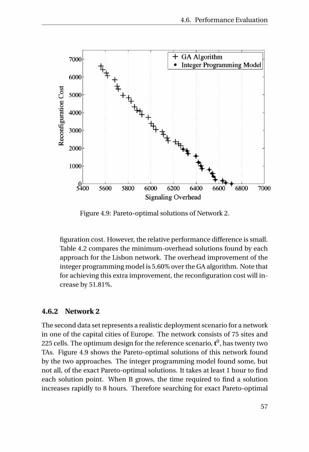
4.6. Performance Evaluation
Figure 4.9: Pareto-optimal solutions of Network 2.
figuration cost. However, the relative performance difference is small.Table 4.2 compares the minimum-overhead solutions found by eachapproach for the Lisbon network. The overhead improvement of theinteger programming model is 5.60% over the GA algorithm. Note thatfor achieving this extra improvement, the reconfiguration cost will in-crease by 51.81%.
4.6.2 Network 2
The second data set represents a realistic deployment scenario for a networkin one of the capital cities of Europe. The network consists of 75 sites and225 cells. The optimum design for the reference scenario, t0, has twenty twoTAs. Figure 4.9 shows the Pareto-optimal solutions of this network foundby the two approaches. The integer programming model found some, butnot all, of the exact Pareto-optimal solutions. It takes at least 1 hour to findeach solution point. When B grows, the time required to find a solutionincreases rapidly to 8 hours. Therefore searching for exact Pareto-optimal
57

4. TRADE-OFF IN TA RECONFIGURATION
4 5 6 7 8 9 10 11 12 13
x 104
0
0.2
0.4
0.6
0.8
1
1.2
1.4
1.6
1.8
2x 10
4
Signaling Overhead
Rec
onfi
gura
tion
Cos
t
GA Algorithm
Figure 4.10: Pareto-optimal solutions of Network 3.
solutions for B ≥ 2000 is not computationally feasible. To get the heuristicPareto-optimal solutions from the GA algorithm in Figure 4.9, the followingparameters are set: POPSIZE = 100, Iteration Limit = 10 and PV-MAX = 20.The PV matrix is set to a size of 700-by-700, which gives a resolution of 10.55and 9.59 units in overhead and cost, respectively. The GA computation tookabout 10 minutes. Below are the observations from the figure.
• The shape of the Pareto frontier, which is the set of all Pareto-optimalsolutions of the signaling overhead and the reconfiguration cost, dif-fers from that of network 1. The curve in Figure 4.9 is close to linear,meaning that to obtain improvement in overhead, the reconfigurationcost scales up proportionally.
• The exact Pareto-optimal solutions available from the integer program-ming model indicate that the Pareto-optimal solutions found by theGA algorithm are of very high quality. The GA algorithm performs verywell and is time-efficient for this network.
58
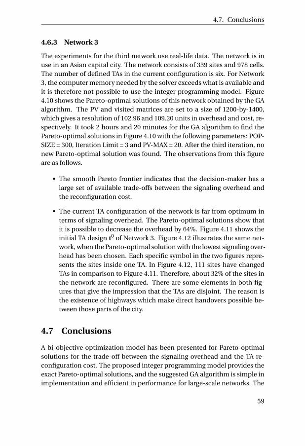
4.7. Conclusions
4.6.3 Network 3
The experiments for the third network use real-life data. The network is inuse in an Asian capital city. The network consists of 339 sites and 978 cells.The number of defined TAs in the current configuration is six. For Network3, the computer memory needed by the solver exceeds what is available andit is therefore not possible to use the integer programming model. Figure4.10 shows the Pareto-optimal solutions of this network obtained by the GAalgorithm. The PV and visited matrices are set to a size of 1200-by-1400,which gives a resolution of 102.96 and 109.20 units in overhead and cost, re-spectively. It took 2 hours and 20 minutes for the GA algorithm to find thePareto-optimal solutions in Figure 4.10 with the following parameters: POP-SIZE = 300, Iteration Limit = 3 and PV-MAX = 20. After the third iteration, nonew Pareto-optimal solution was found. The observations from this figureare as follows.
• The smooth Pareto frontier indicates that the decision-maker has alarge set of available trade-offs between the signaling overhead andthe reconfiguration cost.
• The current TA configuration of the network is far from optimum interms of signaling overhead. The Pareto-optimal solutions show thatit is possible to decrease the overhead by 64%. Figure 4.11 shows theinitial TA design t0 of Network 3. Figure 4.12 illustrates the same net-work, when the Pareto-optimal solution with the lowest signaling over-head has been chosen. Each specific symbol in the two figures repre-sents the sites inside one TA. In Figure 4.12, 111 sites have changedTAs in comparison to Figure 4.11. Therefore, about 32% of the sites inthe network are reconfigured. There are some elements in both fig-ures that give the impression that the TAs are disjoint. The reason isthe existence of highways which make direct handovers possible be-tween those parts of the city.
4.7 Conclusions
A bi-objective optimization model has been presented for Pareto-optimalsolutions for the trade-off between the signaling overhead and the TA re-configuration cost. The proposed integer programming model provides theexact Pareto-optimal solutions, and the suggested GA algorithm is simple inimplementation and efficient in performance for large-scale networks. The
59
4. TRADE-OFF IN TA RECONFIGURATION
experiments on several real-life networks demonstrated that the character-istic of the Pareto frontier varies by network, and that the proposed GA algo-rithm provides close-to-optimal solutions for large-scale networks in feasi-ble time.
60

4.7. Conclusions
Figure 4.11: The initial TA design t0 of Network 3.
Figure 4.12: A Pareto-optimal solution of Network 3.
61

CH
AP
TE
R
5TRACKING AREA LIST
In LTE, the cells can assign a list of TAs (i.e. Tracking Area List (TAL)) toeach UE, and each cell can potentially assign different TALs to different UEs.This allows more flexible TA configuration and overcomes some of the lim-itations of the standard TA. Before studying the TAL scheme, it is instruc-tive to consider the limitations of the standard TA scheme, which has beenused in the previous chapters. It has already been suggested in the litera-ture [4, 78] that the TAL scheme can prevent the frequent updates that arisewhen a UE keeps hopping between two or more adjacent cells in differentTAs (the so called ping-pong effect). Further, TAL can solve the problem ofhigh uplink traffic due to simultaneous updates of a large number of UEscrossing a TA boundary (the train scenario). In this chapter, in addition tothese two problems, the symmetric and transitive properties of the standardTA scheme are compared with the flexible configuration of TAL. Later in thechapter, the challenges in applying the TAL scheme in a large scale networkare explained.
This chapter aims to shed light on the idea of TAL, which is explored fur-ther in the coming chapters. Part of the discussion presented in this chapterhas been published in [81].
5.1 Limitations of Standard TA
As has already been explained in this dissertation, in the standard TA scheme,cells are grouped into mutually disjoint sets, each being a TA. A cell belongsto exactly one TA, and each UE is registered to only one TA. The followingsubsections explain some well-known drawbacks of this scheme.
63

5. TRACKING AREA LIST
Figure 5.1: (a) ping-pong effect, (b) generalized ping-pong effect.
5.1.1 Ping-Pong Effect
It is often the case that UEs at the border of neighboring TAs move back andforth between the two or three neighboring TAs. These phenomena, shownin Figure 5.1, are referred to as the ping-pong and the generalized ping-pongeffects, respectively [46]. Apart from the mobility of the UEs, fading of the ra-dio channel can also cause the ping-pong effect. The effect causes excessiveTAUs and accounts for a non-negligible portion of the total TAU signalingoverhead.
In the standard TAU and paging scheme, no matter how the TAs are de-signed, the ping-pong effect exists between two neighbor TAs, and some-times even between three neighbor TAs of a corner. In general, reducing theping-pong effect can significantly improve the performance of a networkand has therefore received considerable attention in the literature [36, 46,70]. However, most of the proposed schemes for reducing this effect intro-duce a large paging overhead.
5.1.2 Massive Mobility Signaling Congestion
If a large number of UEs simultaneously move into a hotspot cell (e.g. UEsin a train arriving to a platform [78]), there is a risk of increased network loadcaused by excessive TAU from the UEs in a short period of time. Figure 5.2shows the TAU storm, when a train passes a TA border. This is an undesir-able situation from the network standpoint, as it could decrease the qualityof service (QoS) in the cell and create signaling resource congestion [74].
64

5.1. Limitations of Standard TA
Figure 5.2: Example of TAU storm at the border of two TAs.
In addition to the train scenario, with the standard TA scheme, there areseveral types of mobility patterns that may cause TAU congestion. For exam-ple, in densely populated cities, there is a drastic difference in the mobilitybetween day and night. A very large number of UEs moving concurrentlyinto a central area (typically early morning of a weekday) may generate ex-cessive signaling around the center [3, 74, 78]. Conversely, heavy pagingmay occur as a result of massive and almost static UEs simultaneously lo-cated at some hotspot (e.g., a large stadium). The problem of massive mo-bility signaling congestion is extensively considered and is presented in thisdissertation in Chapters 8 and 9.
5.1.3 Symmetric Property
For the standard TA scheme, the following implication exists. If cell A con-siders B in the same TA, then cell B also considers A in the same TA. If cellscould have different perspectives towards each other, then this flexibilitymight lead to a lower signaling overhead.
• Example: Consider A and B only from the network in Figure 5.3. TheTA design either considers these two cells in the same TA, or separatesthem into two TAs. Based on (2.2), in the case that A and B are in thesame TA, the signaling overhead is c1 given in (5.1), and when A andB are in separate TAs the signaling overhead is c2 given in (5.2).
65

5. TRACKING AREA LIST
Figure 5.3: A three-cell network.
c1 =αcp (uA +uB ) (5.1)
c2 = cu(hAB +hB A) (5.2)
c3 = cuhAB +αcp uB (5.3)
Although it is not achievable by the standard TA scheme, let us con-sider a design in which all UEs in A perceive that B is in another TA butall UEs in B assume A is in the same TA. In this situation the signalingoverhead is c3 given in (5.3).
In conditions where c1 − c3 > 0 and c2 − c3 > 0 hold, corresponding toαcp uA > cuhAB and cuhB A >αcp uB , the third assumption (5.3) leadsto lower signaling overhead. Thus, when cell A has high cell load, andthere is no or few flow moving from cell A to cell B , and B has lowcell load but high number of moves towards A, there is a potential toreduce the signaling overhead if the cells can break the symmetry intheir view of TA.
5.1.4 Transitive Property
Another implication of the standard TA scheme is transitivity: if cells A andB are in the same TA, and cells B and C are in the same TA, then cells A andC must also be in the same TA.
• Example: Consider Figure 5.3 and two TA configurations for this net-work. The first configuration puts all three cells in one TA. Based on(2.1), this configuration results in matrix S1(t) given in (5.4). In the
66

5.1. Limitations of Standard TA
second configuration, A and B are in the same TA, while C forms itsown TA, which results in matrix S2(t) given in (5.5). The correspondingsignaling overheads from (2.2), c4 and c5 are given in (5.6) and (5.7),respectively.
S1(t) = 1 1 1
1 1 11 1 1
(5.4)
S2(t) = 1 1 0
1 1 00 0 1
(5.5)
c4 = 2αcp (uA +uB +uC ) (5.6)
c5 =αcp (uA +uB )+cu(hAC +hC A +hBC +hC B ) (5.7)
Let us assume that a design represented by matrix S3(t) given in (5.8)can be created, disregarding the fact that it is not achievable using thestandard TA scheme. The signaling overhead of matrix S3(t) is equalto c6 in (5.9).
S3(t) = 1 1 0
1 1 10 1 1
(5.8)
c6 =αcp (uA +2uB +uC )+cu(hAC +hC A) (5.9)
In situations where c4 −c6 > 0 and c5 −c6 > 0, meaning thatαcp (uA +uC ) > cu(hAC +hC A) and αcp (uB +uC ) < cu(hBC +hC B ), de-signs (5.4) and (5.5) have higher signaling overhead compared to de-sign (5.8). This example illustrates that there is a potential for reducingthe signaling overhead if the transitivity condition can be relaxed.
Generally, in the standard TA scheme, there are three properties for anyS(t) matrix:
67

5. TRACKING AREA LIST
• S(t) is a binary matrix, where si j (t) represents whether or not two cellsare in the same TA.
• S(t) is a symmetric matrix, representing the obvious fact that if cells iand j are in the same TA, then cells j and i are also in the same TA (Ifsi j (t) = 1, then s j i (t) = 1).
• S(t) has the transitive property, meaning that whenever cells i and jare in the same TA, and cells j and k are in the same TA, then i and kare also in the same TA (If si j (t) = si k (t) = 1 then s j k (t) = 1).
5.2 Tracking Area List
There have been extensive discussions in 3GPP regarding the preferred TAscheme for LTE systems. The standard TA scheme, which consists of non-overlapping static TAs, as exists in GSM was used in earlier deployments.However, there are newer schemes that have the potential to avoid ping-pong effects, distributing the TAU load more evenly across cells and reduc-ing the overall TAU signaling overhead [88].
Introducing the concept of TAL gives more flexibility to the operators intheir TA management. Some earlier candidate schemes that were discussedin the literature are as follows [91]:
• Overlapping TA: In this scheme, one cell is assigned to a list of overlap-ping TAs and a UE is assigned only to one TA of the cell’s list. The UEdoes not perform a TAU while moving to a cell which has the assignedTA in its list.
• Multiple TAs: In this scheme, a cell belongs to only one TA, but a UEcan be assigned more than one TA using a list. If one UE is assigned alist of TAs, the UE does not perform TAUs when it crosses the bound-aries between these TAs. The TAs in this scheme are non-overlapping.
The more common scheme, which is also considered for TAL in this dis-sertation, is that a UE can be assigned a list of TAs, and a cell is able to assigndifferent TALs to different UEs. A UE receives a TAL from a cell, and keeps ituntil it moves to a cell that is not included in its TAL. The location of a UE isknown to the MME to the granularity of its TAL.
There are two general candidate architectures for the TAL assignmentof LTE networks. One is to design TALs for UEs, meaning that the network
68
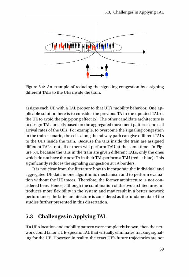
5.3. Challenges in Applying TAL
Figure 5.4: An example of reducing the signaling congestion by assigningdifferent TALs to the UEs inside the train.
assigns each UE with a TAL proper to that UE’s mobility behavior. One ap-plicable solution here is to consider the previous TA in the updated TAL ofthe UE to avoid the ping-pong effect [5]. The other candidate architecture isto design TAL for cells based on the aggregated movement patterns and callarrival rates of the UEs. For example, to overcome the signaling congestionin the train scenario, the cells along the railway path can give different TALsto the UEs inside the train. Because the UEs inside the train are assigneddifferent TALs, not all of them will perform TAU at the same time. In Fig-ure 5.4, because the UEs in the train are given different TALs, only the oneswhich do not have the next TA in their TAL perform a TAU (red → blue). Thissignificantly reduces the signaling congestion at TA borders.
It is not clear from the literature how to incorporate the individual andaggregated UE data in one algorithmic mechanism and to perform evalua-tion without the UE traces. Therefore, the former architecture is not con-sidered here. Hence, although the combination of the two architectures in-troduces more flexibility in the system and may result in a better networkperformance, the latter architecture is considered as the fundamental of thestudies further presented in this dissertation.
5.3 Challenges in Applying TAL
If a UE’s location and mobility pattern were completely known, then the net-work could tailor a UE-specific TAL that virtually eliminates tracking signal-ing for the UE. However, in reality, the exact UE’s future trajectories are not
69

5. TRACKING AREA LIST
Figure 5.5: An example of TAL.
available, and models and algorithms for TAL configuration at a more aggre-gated level are required [20]. In the TAL schemes discussed in this disserta-tion, both UEs and cells are assigned a TAL. A UE receives a TAL from a cell,and keeps the TAL until it moves to a cell that is not included in any TA onthe list. The UE location is known to the MME to the granularity of the TALallocated to that UE.
• Example: In Figure 5.5, TAL1 consists of TA1, TA2, TA3 and TA4, andTAL2 consists of TA2, TA7 and TA8. Assume that the network givesTAL1 to UE x and TAL2 to UE y. x will only make TAU when passingfrom TA2 to TA7, because x does not have TA7 in its TAL. y will not haveany TAU while moving from TA8 to TA7. Note that if any of these UEswere paged, the paging message would be sent to all the cells insidethe UE’s TAL. Therefore, giving a proper TAL to each individual UE canbe very beneficial in TAL design.
By using the TAL scheme, the UEs in one cell may have different TALs,depending on the cells from which the TALs are assigned. This difference ofperspective makes the estimation of signaling overhead difficult. Figure 5.6illustrates two UEs in cell i moving towards cell j . The UEs are assigned dif-ferent TALs which affect the TAU overhead calculation. If cell j is includedin the TAL of cell i , then no TAU overhead is needed for UEs having i ’s listand moving to cell j . This is the case for the upper UE in the figure. TheUE below, on the other hand, does TAU because it does not have j in its list.
70

5.3. Challenges in Applying TAL
Figure 5.6: UEs are assigned to different TALs in one cell.
Similarly, UEs having TALs of other cells, such that the TALs have i but notj , will generate TAU when moving from i to j .
From the discussion above, it can be concluded that in designing TAL fora network, it is highly valuable to have accurate data traces of UEs’ move-ments. Unfortunately, this data is either not available or too expensive toobtain. Also, designing TAL according to traces of UE mobility patterns lim-its the solutions to those specific movement sequences. If the UEs changedtheir movement behavior, which is quite probable, the TALs would becomeinefficient.
71


CH
AP
TE
R
6APPLYING TAL IN CELLULAR
NETWORKS
If the information of each individual UE’s movement and calls were avail-able to the network, then designing an optimum TAL would become trivialand could essentially result in the elimination of the signaling overhead. Thenetwork could give a specific, tailored list to each UE including all the cellsthe UE intends to pass before it will be called. This information, if availableat all, is costly to obtain. Moreover, the validity of the information expiresfast, because the UE trace is the history of the UE’s movement, and the UE’sintention of where and when to move in future is unknown.
Although TAL is expected to overcome some of the limitations of thestandard TA scheme, how to optimize TAL in large-scale networks remainsunexplored. This chapter proposes a signaling overhead calculation for-mula, which takes into account the discussion in Section 5.3. Three schemesare suggested in order to utilize TAL in large-scale networks. The advantagesand disadvantages of each of these schemes are explained.
Here, the naturally arising questions are: What is the potential of reduc-ing the signaling overhead in TAL in comparison to the standard TA scheme?Among all the TAL schemes, which one results in the lowest signaling over-head, and which one is the more practical one to be applied in a large-scalenetwork? A carefully designed evaluation framework is presented to addressthese questions. This chapter is based on the work presented in [81, 82].
73

6. APPLYING TAL IN CELLULAR NETWORKS
6.1 Signaling Overhead Calculation for TAL
To explore the flexibility of TAL, one can consider a TA as small as a singlecell (i.e. no restriction on a given TA layout). Although LTE allows a cell to as-sign UEs different TALs, the assumption here is that a cell will give only onecommon TAL to all UEs being updated in that cell. Inevitably, this imposesrestrictions on the performance of TAL.
Note that for the sake of reusing Equation (2.2), the notations si j (t) andS(t) are kept. However, for the TAL design, the vector t does not exist andthe TAL assignments can be defined in the form of an N ×N matrix. For theTAL design, si j (t) is defined in this dissertation as the proportion of UEs incell i , who have j in their TAL. Thus, the S(t) matrix would contain fractionalvalues which are all between 0 and 1. Although the matrix is no longer bi-nary, Equation (2.2) remains valid. Given a TAL-cell assignment, there maybe several ways to estimate si j (t). In this section, first a one-hop estimationis considered, and then the idea is extended to two hops.
6.1.1 One-hop Estimation
The uncertainty factor in calculating si j (t) stems from the fact that UEs incell i may be assigned to TALs of cells other than cell i . This happens be-cause some UEs move to cell i , without updating to the TAL of i , becausetheir TALs include i . To calculate si j (t) in the one-hop estimation, the im-pact of neighbor cells of i is considered. The formula is shown in (6.1). Thedenominator shows an estimation of the total number of UEs in i . The sec-ond term in the denominator calculates the number of UEs moving to iwithout being updated by cell i , while ui estimates the number of UEs in celli having the TAL of i . The numerator estimates the number of UEs which arelikely to have j in their TALs. Parameter li j is 1 if j is in the TAL of i and 0otherwise. The neighbors of i having i in their TAL form the Qi set. Factorγ represents the probability of UEs entering cell i and having been updatedin Qi . The parameter γ can be obtained from the statistical knowledge of alarge population in the network.
• Example: In Figure 6.1 only the impact of neighbor cells of i are con-sidered, and the orange cells represent the neighbors containing i intheir TAL. If ln1i = ln2i = 1, then Qi = {n1,n2}.
74

6.1. Signaling Overhead Calculation for TAL
Figure 6.1: Parts of a network involved in one-hop estimation of the si j (t).
si j (t) = ui li j +γ∑
n∈Qihni ln j
ui +γ∑
n∈Qihni
(6.1)
The standard TA scheme can be used as a baseline for validating (6.1).For all n ∈ Qi , because Qi is the set of neighbors of i having i in their TAL,lni = 1. Also, for the standard TA scheme all the cells inside one TA are as-sumed to have the same TAL. If li j = 1 then by the transitive relation in thestandard TA scheme ln j = 1 for all n ∈Qi , and hence si j (t) = 1. If li j = 0 thenagain, due to transitivity, ln j = 0 for all n ∈ Qi , and hence si j (t) = 0. Thisleads to the conclusion that the parameter γ does not play any role in thesi j (t) calculation of the standard TA scheme and si j (t) = li j , for all i , j ∈N .
Based on Equation (6.1), because the TAL of each cell contains that cell,the values on the diagonal of S(t) are always equal to one.
6.1.2 Two-hops Estimation
To extend the estimation to two hops, the impact of the neighbors of neigh-bors should be also included in the calculation. This increases the accuracyof the S(t) estimation. In Equation (6.2) two hops are considered. The de-nominator shows an estimation of the total number of UEs in i . The totalnumber of UEs in cell i is estimated by the sum of cell load of i and the UEsentering i with i in their TAL. The numerator of (6.2) gives the number of
75

6. APPLYING TAL IN CELLULAR NETWORKS
Figure 6.2: Parts of a network involved in two-hops estimation of the si j (t).
UEs in i estimated to have j in their TALs. Parameter li j is 1 if j is in the TALof i and 0 otherwise.
si j (t) = ui li j +γ1∑
n∈Qihni ln j +γ2
∑n∈Qi
∑p∈Qni
mi n(hpn ,hni )lp j
ui +γ1∑
n∈Qihni +γ2
∑n∈Qi
∑p∈Qni
mi n(hpn ,hni )(6.2)
As before, the neighbors of i having i in their TAL form the Qi set. Nota-tion Qni is the set of neighbors of n ∈ Qi having both n and i in their TALs.In most of the cases, i ∈Qni , because as long as the neighborhood definitionis defined in both directions, i is considered as the neighbor of neighbor ofi . While UEs move from the cells in Qni to n and thereafter to i , there will beno TAU.
• Example: In Figure 6.2 the impact of neighbors of neighbors is illus-trated. The TAL of orange cells contain i and the connected cells fromthe first-hop neighbors containing i . By assuming ln1i = li n1 = ln2i =lp1n1 = lp1i = lp1n2 = lp3n2 = lp3i = ln1n2 = 1 in the figure, one concludesQi = {n1,n2}, Qn1i = {i , p1}, and Qn2i = {n1, p1, p3}, and therefore theassigned TAL of UEs in cell i can be the TAL of i ,n1,n2, p1 or p3.
Factor γ1 represents the probability of UEs entering cell i having beenupdated in Qi . Similarly, γ2 is the fraction of UEs entering cell i and have
76

6.2. How to Design TAL?
a TAL which is assigned by some cell in Qnk i with nk ∈ Qi . The reason forpicking the minimum value between hpn and hni in the last term is to avoidoverestimating the effects of UEs entering i .
It can be concluded from the definitions of γ1, γ2 and (6.2) that:
γ1 +γ2 ≤ 1 (6.3)
γ2 ≤ γ1
The constraints in (6.3) conclude that γ2 ≤ 0.5. It should also be con-sidered that not all combinations would be feasible. To give one example,γ1 = γ2 = 0.5 is not a valid assumption, because it represents that for eachcell, the impact of the second-hop cells (not including the cell itself) is asgreat as the first-hop cells.
6.2 How to Design TAL?
The aim is to find a scheme to design a TAL configuration for a cellular net-work using the available data. In this section, the following three schemesare introduced and explained in detail.
Scheme 1. TAL design independent from UE tracesScheme 2. An intuitive rule of thumbScheme 3. TAL design based on UE traces
All the schemes are constructed based on the objective of improving thetotal signaling overhead.
6.2.1 Scheme 1: TAL Design Independent from UE Traces
For allocating and assigning TAL independently from UE traces, the onlyavailable information is the load of each cell and the number of handoversbetween cell pairs. In Section 6.1, simple formulas were defined for esti-mating all si j (t) values of the S(t) matrix, considering one or two hops. Thedefinition of the li j parameter in the formulas requires a TAL assignment.Thus, the problem is narrowed down to the challenge of finding a TAL as-signment resulting in an estimated S(t) matrix which improves the total sig-naling overhead calculated by Equation (2.2).
Because UEs in one cell can be assigned different TALs, it is clearly notpossible to set each element of S(t) completely independently from the other
77

6. APPLYING TAL IN CELLULAR NETWORKS
Figure 6.3: An example of the dependency between elements of S(t).
elements. Also, it has already been mentioned in Section 6.1 that the si j (t)values in the TAL can be fractional.
• Example: One can observe from Figure 6.3 that by adding or omittingj from the TAL of i , not only si j (t), but sp1 j (t), sp2 j (t), s j m1 (t), s j m2 (t)and s j m3 (t) can all change in the S(t) matrix.
The following local search algorithm is developed to make the TAL as-signment of each cell, considering the effects on the other cells.
6.2.1.1 Local Search Algorithm
The algorithm iteratively updates the TAL assignment of each cell. The basicoperation of the algorithm is to modify the TAL of one cell at a time, by ei-ther deleting or adding one of the elements in the TAL. Then, depending onwhether one or two hops are used in the algorithm, Equation (6.1) or (6.2)is used respectively to estimate the S(t) matrix, which in turn gives the totalsignaling overhead. This is repeated until no additional change results inany improvement.
The local search algorithm is formalized in Algorithm 3, in which the ini-tial solution given to and returned by the algorithm is denoted by t al l , andthe algorithm considers one-hop calculation. The optimal standard TA con-figuration can be used as the starting TAL assignment of the network. Thismeans that the cells which belong to the same TA are given a list containingall the cells in the TA. Of course, with this solution, the S(t) matrix is binary,
78

6.2. How to Design TAL?
Algorithm 3 Local Search for TAL Allocation.
1: t al 0 = t∗2: t al∗ = t al 0; c∗SO = cSO (t al∗)3: repeat4: δ= 0, c
pSO = c∗SO
5: for all i ∈N do6: for all j ∈N do
7: t al l = t al∗ and At al l = At al∗
8: if j ∈ t al li then
9: t al li = t al l
i \ { j }, Update At al l
i and si j
10: for all p ∈ t al li do
11: if p ∈ t al lj then
12: Update s j p13: end if14: if j ∈ t al l
p then15: Update sp j16: end if17: end for18: if cSO (t al l ) < c∗SO then
19: t al∗ = t al l and c∗SO = cSO (t al∗) and At al∗ = At al l
20: else21: t al l = t al∗, At al l = At al∗
22: end if23: end if24: if j ∈ At al
i then
25: t al li ← {t al l
i , j }, Update At al l
i and si j
26: for all p ∈ t al li do
27: if p ∈ t al lj then
28: Update s j p29: end if30: if j ∈ t al l
p then31: Update sp j32: end if33: end for34: if cSO (t al l ) < c∗SO then
35: t al∗ = t al l , c∗SO = cSO (t al∗), At al∗ = At al l
36: else37: t al l = t al∗, At al l = At al∗
38: end if39: end if40: end for41: end for42: δ= c
pSO − c∗SO
43: until δ∗ = 0
44: return t al l
79

6. APPLYING TAL IN CELLULAR NETWORKS
and is by definition, equal to the matrix obtained from the condition statedin (2.1).
At line 8, the algorithm checks whether or not j should be in the TAL ofi . If j belongs to the list of i , the algorithm removes this cell at line 9, andif it does not belong to the list of i , but it is adjacent to the TAL of i , thealgorithm adds it to the list of i at line 25. All the neighbor cells to the TAL ofi are stored in At al
i . When j is added or removed from the TAL of i , row At ali
of the matrix At al is updated by the algorithm.
According to the discussion in Section 6.2.1 and Figure 6.3, it can be con-cluded that by adding/removing only one cell j to/from the TAL of anothercell i , there are three elements in the S(t) matrix which should be updated,in the case of one-hop calculation:
•si j (t)•sp j (t) for all p ∈ t ali ∩ t al j
•s j p (t) for all p ∈ t ali ∩ t alp
The algorithm changes these elements of S(t) and calculates the signal-ing overhead. If the change results in a lower signaling overhead, then thechange is kept; if it results in a higher signaling overhead, the previous con-figuration is again active, and the change is discarded. By repeating thisprocedure for every (i , j ) pair, a modified TAL will be defined for each cell.The algorithm iterates until no more improvement is possible. Note thatthe algorithm does not achieve the optimum TAL design, but rather aimstowards an improved configuration which should result in a lower total sig-naling overhead compared to the standard TA scheme.
6.2.1.2 Advantages
• The scheme does not require any information regarding the UE traces.The same input data for designing a standard TA scheme can also beused here.
• The scheme considers the impact of adding or omitting a cell fromthe list of other cells on either one-hop or two-hops cells; thereforethe calculation tends to take care of the challenge explained in Section5.3.
80

6.2. How to Design TAL?
6.2.1.3 Disadvantages
• The scheme is based on the si j (t) formulas suggested in (6.1) and (6.2).Each cell has its own value of γ. However, the average estimation ofthis value over the network is considered in the formulations. It is hardto approach a good average estimation of γ, which influences the TALdesign and the resulting signaling overhead. In the two-hops formula,a good estimation of the ratio between γ1 and γ2 is also important.
• Applying the scheme by considering two-hops formulation has a ratherhigh complexity of calculations.
• The starting point in the algorithm of the scheme has an impact onthe final result. A reasonable available starting point is to use the op-timum standard TA configuration. This requires obtaining the opti-mum standard TA design before starting the algorithm.
6.2.2 Scheme 2: An Intuitive Rule of Thumb
The flexibility of TAL compared to the standard TA scheme is that S(t) is notnecessarily binary nor symmetric. If one considers a network with only twocells (e.g. cells i and j in Figure 6.1 and ignoring the rest). There are twochoices for designing the TAL of cell i :
1. t ali = {i }In this case, the signaling overhead resulting from cell i is cuhi j . Thismeans that all the flow moving from i to j should have a TAU, becausej is not included in the TAL of i .
2. t ali = {i , j }Here, the signaling overhead resulting from cell i is αcp ui , meaningthat if a UE is paged in i , there will be paging in cell j , but there is noTAU for the UEs moving from i to j .
Thus, in order to minimize the signaling overhead resulting from cell i , thefollowing decision can be made:
li j ={
1 if αcp ui < cuhi j ,0 otherwise.
(6.4)
If αcp ui < cuhi j , then it is desirable for i to include j in its TAL. Thesame logic can be applied for designing the TAL of cell j . This principle is
81

6. APPLYING TAL IN CELLULAR NETWORKS
generalized to the whole network by separately considering each (i , j ) pairin the network.
6.2.2.1 Advantages
• The scheme is simple and easy to apply on a large-scale network. Itoften gives a good TAL assignment. That is why it is named a rule ofthumb for designing TAL.
• The scheme does not require any information other than the load andhandover of the cells. It does not even depend on the standard TAconfiguration or tuning of any parameter.
• The scheme has very low computational complexity.
6.2.2.2 Disadvantages
• The main disadvantage of the scheme is that it only searches amongthe one-hop neighbors of a cell to be included in the TAL of that cell.Thus, the maximum length of a cell’s TAL is the number of neighborsof the cell plus one. This limitation becomes critical if reducing theTAU overhead is prioritized over reducing the paging overhead (i.e.cu ≫ cp ).
• In this scheme, each cell "selfishly" optimizes the signaling overheadaccording to its own data and does not consider the joint effect of theother cells’ TALs.
6.2.3 Scheme 3: TAL Design based on UE Traces
In the previous two schemes, the TAL design has been based on the load andhandover of cells for a time duration. If possible, it would be desirable toutilize UE traces in designing a TAL. With the earlier cellular technologies,getting the traces of idle UEs was an extremely costly and unfeasible pro-cedure. However in LTE, there are some possibilities for collecting a smallportion of UE traces. One is the existence of UEs using GPS-featured ap-plications in the network. Another possibility is to apply the TAL scheme,which is explained below and which collects a set of UE traces.
82

6.2. How to Design TAL?
Figure 6.4: An example of how to collect part of UE traces.
6.2.3.1 Collecting UE traces by the TAL scheme
Since a cell is able to give different TALs to different UEs, it becomes feasibleto collect a fraction of UE traces. If all cells in a network update a specific UEby giving it a TAL which only contains the updating cell, then the networkcan trace that specific UE. The idea is clarified by the following example.
• Example: In Figure 6.4, first let us consider that x and y follow the gen-eral configuration of the network, and are assigned to TAL1 and TAL2,respectively. In this case, none of the UEs will perform an update forthe UE trace shown in the figure. In the next step, consider that both xand y are two specific UEs, for which the network collects their traces.In this case, every cell gives TAL of a single cell to x and y, and not TAL1and TAL2. The TALs of x and y always consist of one cell, which is thecurrent serving cell. Therefore, by all the updates, the trace 2-5-7 canbe collected for x and the trace 9-8-6 can be collected for y.
The price of collecting a portion of UE traces is the number of updatesthat the selected UEs create. Note that for these selected UEs, there is nopaging overhead.
6.2.3.2 Optimization Algorithm
Unlike the other two schemes, the load and handover of the cells are notused in the optimization algorithm of this scheme. Instead, a portion of UE
83

6. APPLYING TAL IN CELLULAR NETWORKS
traces is considered as the input data. The algorithm goes through theseUE traces and considers whether adding or omitting a cell from the TALof another cell will potentially improve the total signaling overhead or not.The algorithm uses the same basic TAL-modification operation as in Algo-rithm 3, explained in the first scheme. The difference is that the collectedUE traces are used in the signaling overhead estimation. The result is theoptimized TA assignment for the available UE traces, and the solution canbe applied to the entire network. Of course, having 100% of the UE traces,could lead to a close-to-optimum TAL assignment for the network.
6.2.3.3 Advantage
• The scheme takes advantage of the tracing possibility allowed by theflexibility of TAL.
6.2.3.4 Disadvantage
• In order to obtain a reasonable result for this scheme, the network hasto trace some UEs at the accuracy of the cell level. This may cause toomuch signaling if the sampling percentage is large.
6.3 Performance Evaluation of the Proposed TALSchemes
The performance of a TAL scheme is always dependent on the UE tracesinside the network. In order to have a fair comparison between the stan-dard TA and the proposed TAL schemes, all the schemes are applied to thesame UE-traces scenario. A UE-traces scenario is a set of UE traces and callarrivals for a specific time period in a network, matching the cell load andhandover. One set of cell load and handover data, can have many matchingUE-traces scenarios. The UE-traces scenario is dependent on the chosenmobility model, including the amount and speed of each UE’s movement.
There is an extensive amount of research on mobility models using an-alytical and simulation approaches [27, 33, 34]. However, the study of UEsmobility behaviors is out of the scope of this dissertation, and hence themethods applied for generating the UE-traces scenario used for the perfor-mance evaluation, and aggregating the data from it, are explained in Ap-pendix B.
84

6.4. Numerical Results
The standard TA and TAL schemes can be applied to the same UE-tracesscenario and their performance can be compared to each other. For mostof the schemes, however, the aggregated data in load and handover are theinput. One method for the accurate calculation of the total signaling over-head is to directly count the total number of TAU and paging signalings inthe UE-traces scenario.
6.3.0.5 Signaling Overhead Calculation
Assuming that each cell has received the TAL of the starting cell, the TAL ofeach UE is known in all the time intervals through following the UE trace.Each time a UE moves from a cell which is not included in the UE’s TAL,the TAU cost cu is added to the total signaling overhead. Depending on thelength of the TAL, denoted by Lt al , at the time of paging, (Lt al − 1)× cp isadded to the total signaling overhead. When the TAL of a UE consists of onlythe serving cell, the paging overhead for the UE is zero. Similarly, in longerTALs, the serving cell should be excluded from the paging overhead. This isthe reason why the value one is reduced from Lt al in the paging overheadcomputation. This procedure is repeated for all the UEs in the UE-tracesscenario. Thus, the obtained total signaling overhead is the exact value forthat UE-traces scenario.
6.4 Numerical Results
The numerical study that follows is based on the data from the Lisbon net-work. Ten UE-traces scenarios were generated by using the method in B.1which resemble one available set of data of the cell load and handover in onehour. The number of UEs in all UE-traces scenarios is 25,000. The one-hourtime period is divided into 60 equal time intervals. Thus, the time granular-ity is 1 minute.
The dimension of the scenario matrices in all ten scenarios is 25,000×60. The parameter α is 0.0167, which means 1.67% of the UEs are paged inthe UE-traces scenarios. The possibility of a UE being called several timesduring the one hour time period is also considered. This is done by allowingthe UE which was called previously to enter the random call selection for itsother time slots. Among the elements of the scenario matrix, the number ofactive UEs scaled by the time proportion is 5% of the total cell load. Whilea UE is in the active state, there is no signaling overhead for that UE duringthe call. The average length of the call durations is assumed to be 3 minutes.
85

6. APPLYING TAL IN CELLULAR NETWORKS
Table 6.1 gives the numerical assumptions and values for this performanceevaluation.
The cell load and handover data are aggregated from each UE-traces sce-nario, based on the method explained in B.2. The aggregated cell load andhandover are comparable to those in the original data. The assumptions arethat cu = 1 and cp = 0.1. The optimum standard TA configuration is com-puted by CPLEX [60] using the model in [109] for each UE-traces scenariodata set. TAL configuration is at the granularity of the cell level.
Table 6.1: Numerical assumptions and values for performance evaluation.
Parameter Description Valuesα Call intensity factor 0.0167cp Cost of a single paging 0.1cu Cost of a single TAU 1N Number of cells 164T Number of TAs [11 - 30]
The three schemes presented earlier in this chapter for designing TALare implemented in MATLAB. The computations are run on an Intel Core 2Duo of 2.1 GHz.
6.4.1 Standard TA Design
The signaling overhead of the standard TA (STA) design can be simply com-puted from the aggregated cell load and handover. As a baseline for the per-formance evaluation, the signaling overheads of the STA design were com-puted for the ten UE-traces scenarios based on the method explained in Sec-tion 6.3. The results are presented in Table 6.2. The values for all UE-tracesscenarios are very close, because all are based on the same set of originalcell load and handover data.
6.4.2 Scheme 1: Trace-independent TAL Design
A TAL design based on Scheme 1, which was presented in Section 6.2.1 andconsiders the two-hops estimation, was designed for each UE-traces sce-nario. The local search algorithm took on average 4 minutes to design TALfor one UE-traces scenario. The signaling overheads for this TAL design werecalculated based on 6.3 for all ten UE-traces scenarios. The results are pre-sented in Table 6.3. The observations from comparing the tables can besummarized as follows:
86

6.4. Numerical Results
Table 6.2: Signaling overheads of the STA design.
STAScenario No. TAU Paging Total
1 421 598.7 1019.72 428 549.6 977.63 382 607.2 989.24 449 498.9 947.95 357 622.3 979.36 331 616.1 947.17 325 622.6 947.68 483 494.4 977.49 382 620.4 1002.4
10 363 624.9 987.9
Table 6.3: Signaling overheads of the TAL design obtained from Scheme 1.
TAL1Scenario No. TAU Paging Total
1 71.0 348.8 419.82 49.0 382.4 431.43 64.0 382.4 446.44 64.0 340.2 404.25 48.0 380.2 428.26 43.0 372.8 415.87 36.0 366.2 402.28 49.0 356.5 405.59 64.0 381.1 445.1
10 33.0 375.2 408.2
• The total signaling overheads from the TAL designs are 54% to 58%better than those obtained from the optimal STA designs.
• The TAL algorithm significantly reduces the TAU overhead in relationto the paging overhead. The TAU overheads are reduced by 83% to90% compared to the values obtained from the STA design.
87

6. APPLYING TAL IN CELLULAR NETWORKS
Table 6.4: Signaling overheads of the TAL design obtained from Scheme 2.
TAL2Scenario No. TAU Paging Total
1 317 160.0 477.02 295 162.4 457.43 257 163.6 438.64 312 162.9 474.95 274 165.0 439.06 267 163.0 430.07 285 162.7 447.78 268 157.1 425.19 306 162.8 468.8
10 306 163.9 469.9
6.4.3 Scheme 2: TAL Design based on Rule of Thumb
A TAL design based on the rule of thumb in Section 6.2.2 was designed foreach UE-traces scenario. It took around 10 seconds to design TAL for oneUE-traces scenario. The results of the signaling overhead values are givenfor the ten UE-traces scenarios in Table 6.4. The observations from compar-ing the tables can be summarized as follows:
• The total signaling overheads from the TAL design of Scheme 2 are49% to 56% better than those of the optimal STA designs.
• The rule of thumb in designing TAL significantly reduces the pagingoverhead in relation to the TAU overhead. The paging overheads arereduced by 67% to 73% compared to the values obtained from the STAdesign. This is to be expected because the rule of thumb tends to cre-ate small TALs.
• The total signaling overheads obtained from Scheme 2 are 2% to 15%lower than those obtained from Scheme 1. The exception is ScenarioNo. 3 which resulted in 5% lower total signaling overhead. To comparethe two schemes, one should also consider the speed in reaching theseresults.
88
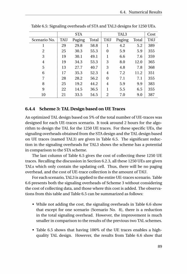
6.4. Numerical Results
Table 6.5: Signaling overheads of STA and TAL3 designs for 1250 UEs.
STA TAL3 CostScenario No. TAU Paging Total TAU Paging Total TAU
1 29 29.8 58.8 1 4.2 5.2 3892 25 30.3 55.3 0 5.9 5.9 3553 19 30.1 49.1 1 6.6 7.6 3594 19 34.3 53.3 3 8.0 12.0 3655 13 27.7 40.7 3 4.8 7.8 3686 17 35.3 52.3 4 7.2 11.2 3517 28 28.2 56.2 0 7.1 7.1 3558 25 19.2 44.2 4 5.9 9.9 3839 22 14.5 36.5 1 5.5 6.5 355
10 21 33.5 54.5 2 7.0 9.0 387
6.4.4 Scheme 3: TAL Design based on UE Traces
An optimized TAL design based on 5% of the total number of UE-traces wasdesigned for each UE-traces scenario. It took around 2 hours for the algo-rithm to design the TAL for the 1250 UE traces. For these specific UEs, thesignaling overheads obtained from the STA design and the TAL design basedon UE traces (named TAL3) are given in Table 6.5. The significant reduc-tion in the signaling overheads for TAL3 shows the scheme has a potentialin comparison to the STA scheme.
The last column of Table 6.5 gives the cost of collecting these 1250 UEtraces. Recalling the discussion in Section 6.2.3, all these 1250 UEs are givenTALs which only contain the updating cell. Thus, there will be no pagingoverhead, and the cost of UE-trace collection is the amount of TAU.
For each scenario, TAL3 is applied to the entire UE-traces scenario. Table6.6 presents both the signaling overheads of Scheme 3 without consideringthe cost of collecting data, and those where this cost is added. The observa-tions from this table and Table 6.5 can be summarized as follows:
• While not adding the cost, the signaling overheads in Table 6.6 showthat except for one scenario (Scenario No. 8), there is a reductionin the total signaling overhead. However, the improvement is muchsmaller in comparison to the results of the previous two TAL schemes.
• Table 6.5 shows that having 100% of the UE traces enables a high-quality TAL design. However, the results from Table 6.6 show that
89
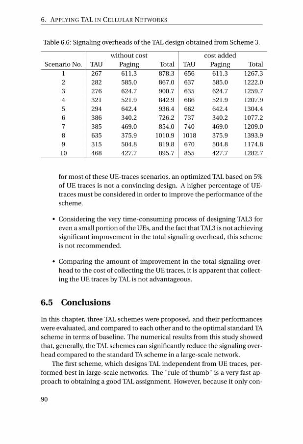
6. APPLYING TAL IN CELLULAR NETWORKS
Table 6.6: Signaling overheads of the TAL design obtained from Scheme 3.
without cost cost addedScenario No. TAU Paging Total TAU Paging Total
1 267 611.3 878.3 656 611.3 1267.32 282 585.0 867.0 637 585.0 1222.03 276 624.7 900.7 635 624.7 1259.74 321 521.9 842.9 686 521.9 1207.95 294 642.4 936.4 662 642.4 1304.46 386 340.2 726.2 737 340.2 1077.27 385 469.0 854.0 740 469.0 1209.08 635 375.9 1010.9 1018 375.9 1393.99 315 504.8 819.8 670 504.8 1174.8
10 468 427.7 895.7 855 427.7 1282.7
for most of these UE-traces scenarios, an optimized TAL based on 5%of UE traces is not a convincing design. A higher percentage of UE-traces must be considered in order to improve the performance of thescheme.
• Considering the very time-consuming process of designing TAL3 foreven a small portion of the UEs, and the fact that TAL3 is not achievingsignificant improvement in the total signaling overhead, this schemeis not recommended.
• Comparing the amount of improvement in the total signaling over-head to the cost of collecting the UE traces, it is apparent that collect-ing the UE traces by TAL is not advantageous.
6.5 Conclusions
In this chapter, three TAL schemes were proposed, and their performanceswere evaluated, and compared to each other and to the optimal standard TAscheme in terms of baseline. The numerical results from this study showedthat, generally, the TAL schemes can significantly reduce the signaling over-head compared to the standard TA scheme in a large-scale network.
The first scheme, which designs TAL independent from UE traces, per-formed best in large-scale networks. The "rule of thumb" is a very fast ap-proach to obtaining a good TAL assignment. However, because it only con-
90

6.5. Conclusions
siders the one-hop neighbors of the TAL of each cell, the design may notperform well for some scenarios, such as in the train scenario for whichit is more reasonable to include more cells forming paths in the TAL. An-other conclusion is that designing TAL based on UE traces results in a designwhich only performs well for the traces collected, and could not be general-ized to a large-scale network.
91


CH
AP
TE
R
7REDUCING SIGNALING OVERHEAD
Since the introduction of the TAL concept for LTE networks, defeating someof the existing limitations of the standard TA design has been expected. How-ever, how to exploit this flexibility in the system, without the existence ofUEs’ mobility traces, was ambiguous. The TAL optimization formulationin this chapter allows a cell to have a collection of potentially overlappingTALs to be assigned to its UEs. Due to the objective function of reducingthe total signaling overhead, the optimal solution is to assign one specificTAL to all UEs being updated in that cell. This takes us back to the prin-ciples of the TAL designs presented in Chapter 6. However, the proposedoverlapping TAL design is able to explore the potential of the list concept toa wider extent compared to what has been done previously. Unlike the pre-vious schemes in which solutions better than the standard TA scheme wereheuristically found, in the current scheme the optimal TAL design in termsof the total signaling overhead is found for a snapshot in time.
The linear program (LP) optimization framework used in this chapter isbased on the use of LTE TALs, which may contain overlapping TAs. To opti-mize the total signaling overhead of the overlapping TAL scheme, the sametrade-off which previously existed in the standard TA scheme on the size ofTAs, now exists for the length of each list in terms of the number of TAs theycontain [78]. Frequent TAUs increase the load in MME and UE battery con-sumption. It also reduces the success rate of paging, as the UE is not ableto respond to paging while it is performing a TAU [110]. On the other hand,long lists would increase the downlink signalings from the MME. Techni-cally, up to 16 TAs per TAL are supported by LTE [5]. This constraint hasbeen added to the formulation of the overlapping TAL scheme.
93

7. REDUCING SIGNALING OVERHEAD
7.1 The Linear Programming Model
A TA as small as a single cell is considered. This means that there will be norestriction on a given TA layout, and it helps to explore the flexibility of theoverlapping TAL to its limit.
The proportional use of TAL ℓ for cell i is denoted by a non-negative op-timization variable xiℓ. The binary indicator aiℓ indicates whether or notthe cell i is in TAL ℓ. The minimization of the total overhead from TAU andpaging can be modeled by the following LP model. The description of nota-tions is also given in Appendix A.
min∑
i∈N
∑j∈N :i = j
cT AU (i , j )+ ∑i∈N
cpag i ng (i ) (7.1a)
s. t.∑ℓ∈L
aiℓxiℓ = 1, i ∈N (7.1b)
cu(hi j∑ℓ∈L
aiℓ(1−a jℓ)xiℓ+h j i∑ℓ∈L
a jℓ(1−aiℓ)xiℓ) =cT AU (i , j ),
(7.1c)
i , j ∈N , i = j
αcp∑ℓ∈L
∑i∈ℓ
∑j∈ℓ,i = j
ui a jℓxiℓ = cpag i ng (i ), i ∈N (7.1d)∑i∈N
aiℓ ≤ NT AL , ℓ ∈L (7.1e)
xiℓ ≥ 0, ℓ ∈L , i ∈N .(7.1f)
The first set of constraints (7.1b) assures that the proportional usage val-ues of TALs in each cell i add up to one. This means that all UEs in each cellwill be assigned a TAL. The second set of constraints (7.1c) computes theTAU between each two different cells i and j in the network. For each or-dered pair i and j , if i but not j is included in TAL ℓ (i.e., aiℓ = 1, a jℓ = 0),then there is a TAU overhead of cuhi j xiℓ between them. The third set ofconstraints (7.1d) calculates the paging overhead of each cell i in the net-work. For any list ℓ in cell i , the overhead for paging UEs in cell j ∈ ℓ isαcp ui scaled by the number of cells in ℓ and the variable xiℓ which standsfor the proportional use of ℓ. The fourth set of constraints (7.1e) assures thatthe length of TALs does not exceed the limit of NT AL , which is the maximumallowable number of TAs in TAL.
94

7.2. Solution Characteristics
7.2 Solution Characteristics
The number of possible lists for each cell is 2N−1, therefore the number ofvariables of the above LP model is exponential in the number of cells N .However, due to the LP formulation, it can be solved efficiently even for alarge number of variables. The following proposition provides a solutioncharacterization.
PROPOSITION 3. At the optimum solution of (7.1), for any cell i ∈N , thereis exactly one ℓ ∈L , such that in xiℓ = 1, and the rest are zeros.
PROOF. Suppose ℓ1 ∈ L and ℓ2 ∈ L (ℓ1 = ℓ2) are both present at the opti-mum solution for cell i , meaning that aiℓ1 = aiℓ2 = 1, xiℓ1 + xiℓ2 = 1, xiℓ1 > 0and xiℓ2 > 0. Then the objective function value for cell i is:∑
j∈N :i = jcuhi j ((1−a jℓ1 )xiℓ1 + (1−a jℓ2 )xiℓ2 )+αcp ui (a jℓ1 xiℓ1 +a jℓ2 xiℓ2 )
Because ℓ1 and ℓ2 are different, there must be at least one cell j ′ thatexists in one list and does not exist in the other list, say a j ′ℓ1 = 1, and a j ′ℓ2 =0. With this observation, the corresponding term in the above sum for j ′
becomes:
cuhi j ′xiℓ2 +αcp ui xiℓ1
Among the two values cuhi j ′ and αcp ui , one has a lower value. Accord-ing to the objective function which is to minimize the total signaling over-head, if cuhi j ′ is lower, then setting xiℓ1 = 0 and xiℓ2 = 1 results in a betterobjective value, and if αcp ui is lower, then setting xiℓ1 = 1 and xiℓ2 = 0 givesa better objective value. However, this is in contradiction to the earlier as-sumption that both xiℓ1 and xiℓ2 are greater than zero at optimum. Thisshows that for any cell i , an extreme solution is optimum for the trade-offbetween update and paging overheads while considering each cell j ′ to beincluded in the list of i or not. The same logic applies in considering morethan two lists in the optimum solution. Hence the conclusion. �
Here, it can be concluded that while using the overlapping TAL schemefor minimizing the total signaling overhead, each cell assigns one specificTAL to all UEs being registered in that cell. What is stated in the propositionis in fact very interesting. Although each cell in the overlapping TAL schemecan use different proportions of TALs, meaning that xiℓ in the formulation
95

7. REDUCING SIGNALING OVERHEAD
can be any non-negative value, due to the objective function in (7.1a), foreach cell there is only one TAL which results in the minimum value of thetotal signaling overhead. This fact sets a proper fundamental for the TALschemes presented in the previous chapter. The solution to the proposedLP model is a lower bound to the performance of the "rule of thumb".
For a snapshot scenario (i.e. given ui and hi j for all i , j ∈ N ), the opti-mum overlapping TAL design solution of the proposed LP model is a lowerbound to the total signaling overhead of any TAL-to-cell assignment for theaggregated data of UEs. This is equivalent to finding the optimum binaryS(t) matrix, in which the symmetric and transitive properties are relaxed.The total signaling overhead of this binary matrix is lower than any frac-tional S(t) matrix. Clearly in the optimum TAL design, for any i , j ∈ N andi = j , the lower value between cuhi j and αcp ui is chosen. Here, it can beconcluded that the optimum overlapping TAL configuration from the LPmodel performs optimally for a limited period of time while considering allUEs have been updated to the TALs of the cells they are located in.
As the UEs are allowed to move freely among the cells included in theirTALs, eventually each cell will contain UEs with different TALs. This chal-lenge has been previously explained in Section 5.3. In the current study thetotal signaling overhead of the optimum TAL design from the LP model mayin reality be far from the one computed in (7.1a), as the scheme is vulnera-ble to the UE traces inside the network. Hence, for performance evaluationof the TAL solution, this vulnerability should be considered.
7.3 Performance Evaluation
To evaluate the performance of the proposed overlapping TAL scheme ona large-scale topology, the Lisbon network is again considered. As splittingthe cells of a site into different TAs is not a common practice, the LP modelis applied at site level.
As the LP model is exponential in the number of sites, applying it to theentire network is a time-consuming process. One solution is to divide thenetwork to smaller sets of sites and apply the model to each set separately.According to constraint (7.1e), the model itself will divide the network intosets of maximum NT AL . The actual value by 3GPP standard NT AL = 16 is sethere. To ensure the optimum division of sites in the network, the integerprogramming model in [109] is used while adding the constraint defined in(7.4). The fact that the site is always included in the lists given by itself is alsoconsidered in the model.
96
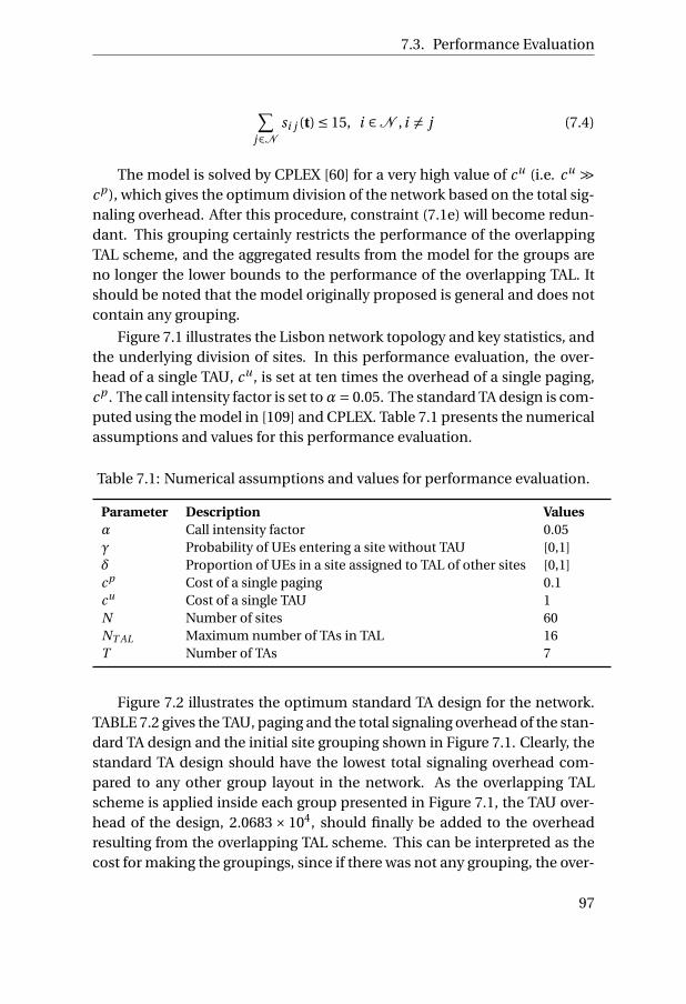
7.3. Performance Evaluation
∑j∈N
si j (t) ≤ 15, i ∈N , i = j (7.4)
The model is solved by CPLEX [60] for a very high value of cu (i.e. cu ≫cp ), which gives the optimum division of the network based on the total sig-naling overhead. After this procedure, constraint (7.1e) will become redun-dant. This grouping certainly restricts the performance of the overlappingTAL scheme, and the aggregated results from the model for the groups areno longer the lower bounds to the performance of the overlapping TAL. Itshould be noted that the model originally proposed is general and does notcontain any grouping.
Figure 7.1 illustrates the Lisbon network topology and key statistics, andthe underlying division of sites. In this performance evaluation, the over-head of a single TAU, cu , is set at ten times the overhead of a single paging,cp . The call intensity factor is set to α= 0.05. The standard TA design is com-puted using the model in [109] and CPLEX. Table 7.1 presents the numericalassumptions and values for this performance evaluation.
Table 7.1: Numerical assumptions and values for performance evaluation.
Parameter Description Valuesα Call intensity factor 0.05γ Probability of UEs entering a site without TAU [0,1]δ Proportion of UEs in a site assigned to TAL of other sites [0,1]cp Cost of a single paging 0.1cu Cost of a single TAU 1N Number of sites 60NT AL Maximum number of TAs in TAL 16T Number of TAs 7
Figure 7.2 illustrates the optimum standard TA design for the network.TABLE 7.2 gives the TAU, paging and the total signaling overhead of the stan-dard TA design and the initial site grouping shown in Figure 7.1. Clearly, thestandard TA design should have the lowest total signaling overhead com-pared to any other group layout in the network. As the overlapping TALscheme is applied inside each group presented in Figure 7.1, the TAU over-head of the design, 2.0683 × 10⁴, should finally be added to the overheadresulting from the overlapping TAL scheme. This can be interpreted as thecost for making the groupings, since if there was not any grouping, the over-
97

7. REDUCING SIGNALING OVERHEAD
Figure 7.1: An illustration of the site groupings for the overlapping TALscheme.
Table 7.2: Signaling overhead comparisons of Figures 7.1 and 7.2. Figure 7.2represents the standard TA design.
TAU Paging TotalDesign in Figure 7.1 2.0683×10⁴ 2.3684×10⁴ 4.4367×10⁴
Design in Figure 7.2 2.3849×10⁴ 1.8603×10⁴ 4.2452×10⁴
lapping TAL model would have had more flexibility in choosing the sites in-cluded in each TAL.
To configure the overlapping TALs for the Lisbon network, the model inSection 7.1 is applied to each group in Figure 7.1. TABLE 7.3 presents the
98

7.3. Performance Evaluation
Figure 7.2: An illustration of the optimum standard TA design.
number of sites, the computed TAU, paging and the total signaling over-head for the overlapping TAL scheme for each group. The last column ofthe table presents the model computing time for each group. The computa-tions are run on Intel Core 2 Duo of 2.1 GHz. One immediate observation isthat the paging overhead accounts for most of the total signaling overheadof each group. The reason is that the network is already divided into groupsof geographically close sites, most of which have a high amount of handoverbetween them, and hence the model is intended to consider those sites ineach others’ TALs.
To give an insight into the design of overlapping TAL designs, TABLE7.4 presents the load and handover of sites in Group 1, which contains four
99
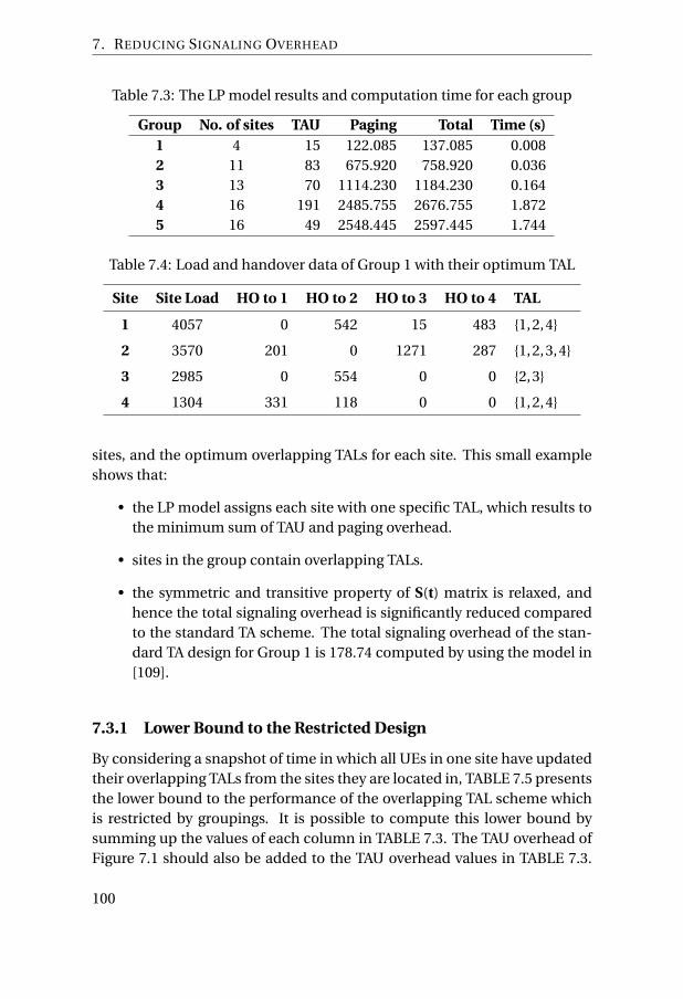
7. REDUCING SIGNALING OVERHEAD
Table 7.3: The LP model results and computation time for each group
Group No. of sites TAU Paging Total Time (s)1 4 15 122.085 137.085 0.0082 11 83 675.920 758.920 0.0363 13 70 1114.230 1184.230 0.1644 16 191 2485.755 2676.755 1.8725 16 49 2548.445 2597.445 1.744
Table 7.4: Load and handover data of Group 1 with their optimum TAL
Site Site Load HO to 1 HO to 2 HO to 3 HO to 4 TAL
1 4057 0 542 15 483 {1,2,4}
2 3570 201 0 1271 287 {1,2,3,4}
3 2985 0 554 0 0 {2,3}
4 1304 331 118 0 0 {1,2,4}
sites, and the optimum overlapping TALs for each site. This small exampleshows that:
• the LP model assigns each site with one specific TAL, which results tothe minimum sum of TAU and paging overhead.
• sites in the group contain overlapping TALs.
• the symmetric and transitive property of S(t) matrix is relaxed, andhence the total signaling overhead is significantly reduced comparedto the standard TA scheme. The total signaling overhead of the stan-dard TA design for Group 1 is 178.74 computed by using the model in[109].
7.3.1 Lower Bound to the Restricted Design
By considering a snapshot of time in which all UEs in one site have updatedtheir overlapping TALs from the sites they are located in, TABLE 7.5 presentsthe lower bound to the performance of the overlapping TAL scheme whichis restricted by groupings. It is possible to compute this lower bound bysumming up the values of each column in TABLE 7.3. The TAU overhead ofFigure 7.1 should also be added to the TAU overhead values in TABLE 7.3.
100

7.3. Performance Evaluation
Table 7.5: Performance comparison of the two schemes in an ideal case.
Overhead Standard TA Designed overlapping TAL Improvement
(lower bound)
TAU 2.3849×10⁴ 2.1091×10⁴ 11.6%
Paging 1.8603×10⁴ 6.9464×10³ 62.7%
Total 4.2452×10⁴ 2.8037×10⁴ 34.0%
TABLE 7.5 compares the overhead values of the standard TA scheme withthe ones obtained by the overlapping TAL design for an "ideal" scenario.
The comparisons show that, ideally, the overlapping TAL design restrictedby groupings is able to significantly (i.e. 34%) improve the performance ofthe signaling overhead in terms of both TAU and paging costs. The reasonfor having 5.4 times more improvement in the paging overhead comparedto the TAU overhead is the elimination of extra paging overhead by relaxingthe symmetric and transitive property of the S(t) matrix.
7.3.2 Empirical Validation of the Design
To justify the effectiveness of the proposed overlapping TALs, the perfor-mance of the scheme is analyzed based on different realistic UE movementscenarios. One advantage of the proposed scheme is the availability of theexact possible TALs that the UEs in one site may have. Let us consider site2 of the small group in TABLE 7.4. As all other sites in the group have {2} intheir TALs, the UEs moving from any of the sites in the group to this site donot perform any TAU. It is obvious that, as time passes, the number of UEshaving the TAL {1,2,3,4} decreases in site 2, as no UE from any of the sites inthe group will update to the TAL of site 2. On the other hand, UEs with thelist of site 2 will not perform any update while moving to any other sites inthe group.
Two methods are used for calculating the signaling overhead of the over-lapping TAL design while considering different UEs’ distribution. Both meth-ods use the aggregated data of UEs, and not any specific UE-trace scenario.Both methods are expected to generate close results, as they, to some extent,share the same fundamentals.
101

7. REDUCING SIGNALING OVERHEAD
0 0.2 0.4 0.6 0.8 10
0.5
1
1.5
2
2.5
3
3.5
4
4.5x 10
4
δ
Sign
alin
g O
verh
ead
TAL TotalTAL TAUTAL PagingSTA TotalSTA TAUSTA Paging
Figure 7.3: Evaluating the overlapping TAL scheme by Method I.
7.3.2.1 Method I
Factor δ represents the proportion of UEs in site i having a TAL other thanthe one assigned by i . Hence, δ= 0 corresponds to the overheads presentedin TABLE 7.5 for the overlapping TAL design. By increasing the value ofδ, the number of UEs with other TALs inside i is increased. The popula-tion of UEs having TAL of site j in i is naturally assumed to be a portionof the handover from j to i . Figure 7.3 compares the signaling overheadsresulting from Method I for different values of δ ∈ [0,1] with the standardTA design. The results show that the proposed overlapping TAL scheme ispromising in terms of reducing the total signaling overhead under differentUE-distribution situations.
7.3.2.2 Method II
The definition of si j given in (6.1) and presented in Section 6.1 is re-usedhere. The parameter li j , which is defined 1 if j is in the TAL of i and 0 oth-erwise, can be obtained from xiℓ solutions of the overlapping TAL design.Figure 7.4 compares the signaling overheads resulting from Method II for
102

7.4. Conclusions
0 0.2 0.4 0.6 0.8 10.5
1
1.5
2
2.5
3
3.5
4
4.5x 10
4
γ
Sign
alin
g O
verh
ead
TAL TotalTAL TAUTAL PagingSTA TotalSTA TAUSTA TAU
Figure 7.4: Evaluating the overlapping TAL scheme by Method II.
all values of γ with the standard TA scheme. As before, the results showthat the proposed scheme is able to improve the performance of the TAL-heterogeneous network.
Figure 7.5 shows that the results from the two methods are very closeto each other, as they both estimate the UE’s distribution based on the loadand handover of the network.
7.4 Conclusions
In this chapter, a linear programming model was proposed to configure over-lapping tracking area lists (TALs) for the purpose of minimizing the totalsignaling overhead of location management in LTE networks. An optimumoverlapping TAL design was allocated to each cell in order to minimize thetotal signaling overhead. It has been proved that the optimum overlappingTAL solution for this problem is that each cell assigns one specific TAL to allUEs being registered in that cell. The LTE constraint on the number of TAsin a list was considered and formulated in the model. Two separate meth-ods were used to evaluate the performance of the overlapping TALs with-
103

7. REDUCING SIGNALING OVERHEAD
0 0.2 0.4 0.6 0.8 10
0.5
1
1.5
2
2.5
3
3.5
4
4.5x 10
4
δ and γ
Sign
alin
g O
verh
ead
Total/ Method I
TAU/ Method I
Paging/ Method I
Total/ Method II
TAU/ Method II
Paging/ Method II
Figure 7.5: Comparison of the overlapping TAL overheads by Method I andII.
out considering any specific UE-trace scenario. The results showed that theoptimized TALs outperform the standard TA scheme in reducing the totalsignaling overhead.
104

CH
AP
TE
R
8SIGNALING CONGESTION MITIGATION
OF THE TRAIN SCENARIO
The signaling congestion problem of the train scenario has been one of themost challenging problems of the standard TA design. The problem has pre-viously been explained in Chapter 5. In this chapter, a modified overlappingTAL scheme is developed to mitigate the signaling congestion due to simul-taneous mass mobility. An LP model which minimizes the number of TAUswhile keeping the total paging overhead lower than some pre-defined limit,is presented.
The congestion mitigation problem of this chapter has also been consid-ered in [74]. The authors of there used a randomized time distribution forthe initiation of the process of cell re-selections to avoid the mass mobilitysignaling congestion. However, their mechanism requires additional con-figuration on the network side to provide the algorithm parameters, whilethe approach presented here uses only existing features of the standard LTEsystems.
One of the main challenges in applying TAL is the estimation of the to-tal signaling overhead of a fully deployed TAL scheme in a large-scale net-work. In the modified overlapping TAL scheme presented in this chapter,the signaling overhead calculation is independent of UE traces. The numer-ical results demonstrate that the proposed model is able to balance the loadin some representative scenarios of massive mobility signaling congestion.The study in this chapter has been appeared in [84].
105

8. SIGNALING CONGESTION MITIGATION OF THE TRAIN SCENARIO
8.1 Modified Overlapping Tracking Area List
In order to mitigate the TAU signaling congestion, some extra paging over-head is introduced, and to mitigate the paging signaling congestion, addi-tion of some extra TAU overhead is inevitable. Therefore, towards avoidingsignaling congestion, the signaling overhead calculation of TAU and pag-ing should be considered, separately. Hence, Equation (2.2) is divided intoEquations (8.1) and (8.2) for TAU and paging signaling overhead, respec-tively.
CU = ∑i∈N
∑j∈N :i = j
cT AU (i , j ) = ∑i∈N
∑j∈N : j =i
cuhi j (1− si j (t)) (8.1)
C P = ∑i∈N
cpag i ng (i ) = ∑i∈N
∑j∈N : j =i
αcp ui si j (t) (8.2)
In Equations (8.1) and (8.2), CU denotes the total TAU signaling over-head, and C P denotes the total paging signaling overhead for a given TA de-sign S(t). In both equations, the middle equality terms relate the parametersto the ones defined in Chapter 7.
In the modified overlapping TAL scheme, each cell uses multiple andoverlapping TALs to be allocated to UEs updating their TALs from the cell.The following subsection explains the modified overlapping TAL schemewith a network of three cells.
8.1.1 An Instructive Example
Figure 8.1 considers the three cells, A, B, and C, along a train path. The op-timum standard TA configuration of this part of the network is one of thefour possible combinations presented in Table 8.1. The parentheses in thesecond column of the table specify different groupings of these three cells.The configuration {(A,C ), (B)} is not a feasible combination, as by construc-tion of this example there is no direct handover from A to C. According toEquations (8.1) and (8.2), the total TAU and paging overheads are calculatedfor each of the four configurations.
If the transitivity condition of the S(t) matrix is relaxed, then Snew (t) ma-trix in (8.3) could become a possible configuration for the example in Figure8.1.
106

8.1. Modified Overlapping Tracking Area List
Figure 8.1: Three cells along a train path.
Table 8.1: Possible TA configurations, CU and C P of the ABC network.
No. Configuration CU C P
1 (A),(B),(C) cu(hAB +hB A +hBC +hC B ) 02 (A,B),(C) cu(hBC +hC B ) αcp (uA +uB )3 (A),(B,C) cu(hAB +hB A) αcp (uB +uC )4 (A,B,C) 0 2αcp (uA +uB +uC )
Snew (t) = 1 1 0
1 1 10 1 1
(8.3)
CUnew +C P
new = cu(hAC +hC A)+αcp (uA +2uB +uC ) (8.4)
The total signaling overhead of Snew (t) is given in (8.4). In the example,hAC = hC A = 0, and CU
new = 0, and hence the Snew (t) configuration has thelowest TAU overhead compared to the configurations in Table 8.1. Assumethat uA ≫ uB and uC ≫ uB (for example considering that there are trainstations in A and C with large number of UEs standing in the platform), thenthe paging overhead C P
new is almost half of the paging overhead of the fourthconfiguration in the table.
This example shows that the transitive property of the S(t) matrix canlimit the performance of the standard TA scheme. Here, it is of interest toshow that the TAL concept has the potential to reduce the overhead by re-laxing this property, and achieving an effect similar to that of Snew (t). How-ever, the challenge in using the list concept is that the UEs in one cell mighthave different lists depending on the cells from which the lists are assigned.One can refer back to the discussion in Section 5.3.
By assuming that each of the cells A, B and C are a separate TA (configu-ration 1) and they can assign UEs with different TALs, Table 8.2 presents the
107

8. SIGNALING CONGESTION MITIGATION OF THE TRAIN SCENARIO
Table 8.2: The list of TALs for each cell in the ABC network of Figure 8.1.
A B C{A} {B} {C }{A,B} {A,B} {B ,C }{A,B ,C } {B ,C } {A,B ,C }
{A,B ,C }
set of all possible TALs for each cell. The TALs assigned by each cell shouldcontain that cell. Cells A and C are not giving TAL {A,C } to their UEs as thereis no direct handover between these two cells; this list only increases thepaging overhead without any improvement in TAU. The table shows thatthe UEs in the ABC network have the possibility to be assigned one of thefollowing six TALs: ({A}, {B}, {C }, {A,B}, {B ,C }, {A,B ,C }).
Let t a denote any TA, and t al denote any TAL of the ABC network; X t at al
is defined as the percentage of the UEs inside each t a having t al as theirlist. Consider the following three equations. Equation (8.5) assures that allthe UEs receiving their lists from A use one of the three candidate TALs of A.Equations (8.6) and (8.7) express the same logic for TAs B and C, respectively.
X AA +X A
AB +X AABC = 1 (8.5)
X BB +X B
AB +X BBC +X B
ABC = 1 (8.6)
X CC +X C
BC +X CABC = 1 (8.7)
By the definition of TAL, the UEs assigned to the list {A,B ,C } can movein the ABC network without any TAU, and they could have also been up-dated to this TAL from any of the cells/TAs. To make the calculation of sig-naling overhead tractable, the restriction that the percentage of assigninga common TAL from different TAs are equal is imposed. This means thatX A
AB = X BAB , X B
BC = X CBC and X A
ABC = X BABC = X C
ABC . Thus, there is no need tocontinue with the superscripts of elements (X t al ).
In the overlapping TAL scheme, the cells inside each TA are assigned alist of overlapping TALs. The cells update the UEs with different TALs intheir lists. The standard TA design is considered as the backbone structure,and the lists are created by different combinations of TAs. In the modifiedoverlapping TAL scheme, the restriction explained in the example is applied.This means that in the modified overlapping TAL scheme, the percentages
108

8.2. An LP Model for the Train Scenario
of assigning a common list from different cells to the UEs in the network areequal.
The biggest difficulty in calculating the signaling overhead was havingUEs with different TALs in one cell. With the assumption on the definitionof X t al and the modified overlapping TAL scheme, the percentage of UEs as-signed to each TAL is known. Therefore, unlike previous studies where thesignaling overhead was calculated by following each UE movement patternand call arrivals or estimated by methods such as the ones presented in Sec-tions 7.3.2.1 and 7.3.2.2, here the TAU and paging overhead formulas givenin (8.1) and (8.2) can be directly used.
From now on and throughout the rest of the dissertation the term over-lapping TAL scheme refers to this modified scheme, and for simplicity theword modified is omitted.
8.2 An LP Model for the Train Scenario
To overcome the signaling congestion in the train scenario, the cells alongthe railway path can assign different TALs to the UEs inside the train, thiswas previously shown in Figure 5.4. As the TAs involved in the train scenarioform a line such as the one in Figure 8.2, the LP formulation has a simplestructure. UE movement occurs only between consecutive TAs along theline. Thus, the TALs contain blocks of consecutive cells, and the formula-tion’s size becomes polynomial in the number of TAs. As numbering the TAsfollows naturally by their positions along the line, for convenience, the po-sition indices are used to refer to TAs. Hence, TA i , i = 1, ..,T , is the i th TAon the line. Each TAL is uniquely identified by its starting and ending TAs,therefore the variable definition is simplified to xi j for the TAL which con-tains all TAs from i to j .
A min-max approach for TAU congestion mitigation is applied, that is,TALs are used to minimize the maximum TAU between all pairs of TAs. Tothis end, an upper bound on the increase of the total paging overhead is nec-essary, as otherwise the optimum would be to completely eliminate TAU byexclusively using the TAL containing all TAs (i.e., as if all cells form one TA).The bound is expressed as βC P , where C P is the total paging overhead ofTA design T , and β is a non-negative parameter denoting the allowed per-centage of increase. An auxiliary variable z is used to denote the maximumTAU between TAs. The min-max TAU optimization problem for the trainscenario can then be modeled by the following LP.
109

8. SIGNALING CONGESTION MITIGATION OF THE TRAIN SCENARIO
Figure 8.2: Definition of variables for the train scenario.
min z (8.8a)
s. t.k∑
i=1
T∑j=k
xi j = 1, k = 1, . . . ,T (8.8b)
cu(hi ,i+1
i∑k=1
xki +hi+1,i
T∑k=i+1
xi+1,k ) ≤ z, i = 1, . . . ,T −1
(8.8c)
αcpT−1∑i=1
T∑j=i+1
j∑k=i
j∑h=k+1
(uk nh +uhnk )xi j ≤βC P , (8.8d)
xi j ≥ 0, i = 1, . . . ,T, j = i , . . . ,T.(8.8e)
The first set of constraints (8.8b) ensures that each TA assigns all its UEswith feasible TALs. For the train scenario, it is sufficient to account for UEmovements between adjacent TAs on the line, as can be seen in (8.8c). In(8.8d), paging is considered for all TA pairs of a line segment, and furtherover all the segments. Apart from the non-negativity requirement, the num-bers of variables and constraints in (8.8) are of O(T 2) and O(T ), respectively.Thus, the optimization approach of the train scenario has low complexity.
While considering two consecutive TAs, i and i +1, it can be easily veri-fied that there are a total of i (T − i +1) TALs containing i , and, among them,i TALs do not contain i+1. Thus, the amount of TAU generated by UE move-ment from i to i +1 depends on the proportional usage levels of the i TALs.The values are strictly between zero and one at optimum, thus not all of theUEs inside the train will perform TAU at a TA boundary, giving the desiredeffect of TAU congestion mitigation.
110
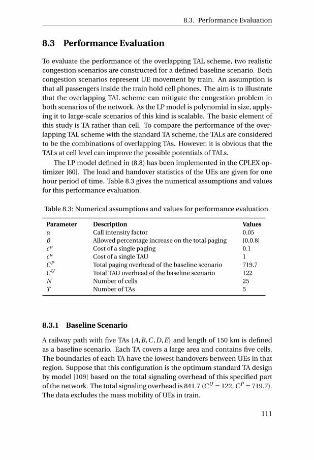
8.3. Performance Evaluation
8.3 Performance Evaluation
To evaluate the performance of the overlapping TAL scheme, two realisticcongestion scenarios are constructed for a defined baseline scenario. Bothcongestion scenarios represent UE movement by train. An assumption isthat all passengers inside the train hold cell phones. The aim is to illustratethat the overlapping TAL scheme can mitigate the congestion problem inboth scenarios of the network. As the LP model is polynomial in size, apply-ing it to large-scale scenarios of this kind is scalable. The basic element ofthis study is TA rather than cell. To compare the performance of the over-lapping TAL scheme with the standard TA scheme, the TALs are consideredto be the combinations of overlapping TAs. However, it is obvious that theTALs at cell level can improve the possible potentials of TALs.
The LP model defined in (8.8) has been implemented in the CPLEX op-timizer [60]. The load and handover statistics of the UEs are given for onehour period of time. Table 8.3 gives the numerical assumptions and valuesfor this performance evaluation.
Table 8.3: Numerical assumptions and values for performance evaluation.
Parameter Description Valuesα Call intensity factor 0.05β Allowed percentage increase on the total paging [0,0.8]cp Cost of a single paging 0.1cu Cost of a single TAU 1C P Total paging overhead of the baseline scenario 719.7CU Total TAU overhead of the baseline scenario 122N Number of cells 25T Number of TAs 5
8.3.1 Baseline Scenario
A railway path with five TAs {A,B ,C ,D,E } and length of 150 km is definedas a baseline scenario. Each TA covers a large area and contains five cells.The boundaries of each TA have the lowest handovers between UEs in thatregion. Suppose that this configuration is the optimum standard TA designby model [109] based on the total signaling overhead of this specified partof the network. The total signaling overhead is 841.7 (CU = 122, C P = 719.7).The data excludes the mass mobility of UEs in train.
111

8. SIGNALING CONGESTION MITIGATION OF THE TRAIN SCENARIO
0 0.2 0.4 0.6 0.80
5
10
15
20
25
Limit on additional paging (parameter β)
Max
imum
TA
U o
verh
ead
at T
A b
ound
arie
s
Standard TA SchemeOverlapping TAL Scheme
Figure 8.3: Evaluating the two schemes for the baseline scenario.
The model (8.8) is applied to the baseline scenario and is run for all βvalues from 0 to maximum. It only takes a few seconds for the solver to cal-culate the optimum proportions of TALs for each β value. Next, the standardTA configurations are designed by minimizing the maximum z, the same ob-jective in Model (8.8), and all the β values. Note that while the β value is 0,all the five TAs are separate in the standard TA configuration, and the equiv-alent solution in the overlapping TAL scheme adapts all the UEs in each TAto contain only that TA in their lists. On the other extreme, when the β valueis maximum, all the five TAs are merged into one in the standard TA config-uration. The overlapping TAL, in this case, gives a list containing all the fiveTAs to every UE. Hence, for the two extremes of the β the optimal standardTA scheme and the overlapping TAL coincide.
The comparison of the standard TA scheme and the overlapping TAL forthe baseline is illustrated in Figure 8.3. As it is explained above, the graphscoincide at the two ends. The figure shows that the standard TA scheme ischanged in four discrete steps. By increasing the limit on the paging over-head, the TAs tend to merge. The behavior of the overlapping TAL schemeis smooth as the proportions of each TAL can be continuously changed. Byallowing 10% addition to the paging overhead, the maximum TAU overhead
112

8.3. Performance Evaluation
Figure 8.4: Congestion Scenario 1.
0 0.2 0.4 0.6 0.8 10
100
200
300
400
500
600
700
Limit on additional paging (parameter β)
Max
imum
TA
U o
verh
ead
at T
A b
ound
arie
s
Standard TA SchemeOverlapping TAL Scheme
Figure 8.5: Evaluating the two schemes for Scenario 1.
at the TA boundaries is reduced by more than 50% with the overlapping TALscheme, while the standard TA scheme can only reduce it by 20%. Note thateven in this uncongested scenario where mass mobility is not considered,the overlapping TAL scheme can significantly perform better than the stan-dard TA scheme by overcoming the transitive restriction explained in Sec-tion 8.1.
113

8. SIGNALING CONGESTION MITIGATION OF THE TRAIN SCENARIO
8.3.2 Congestion Scenario 1
In the first congestion scenario shown in Figure 8.4, a train moves from A toE having 600 passengers on-board.1 After a main station in C , the number ofon-board passengers is reduced to 400. It takes around half an hour for thetrain to pass the whole path (ignoring the time spent at the main station).
The load and handover data from the train scenario are aggregated andadded it to the baseline scenario. All the UEs in the train passing each TAboundary will be added to the corresponding handover. The load is in-creased proportionally to the amount of time the train is spent in each TA.For example, the train spends about 6 min (0.1 hour) in A, therefore the loadof A is increased by 600∗0.1 = 60, due to the fact that the handover and loaddata are given for one hour period of time.
For variousβ values, Figure 8.5 illustrates the behavior of the two schemesin minimizing the maximum TAU. Here the β refers to the additional pag-ing overhead due to the standard TA configurations and the proportions ofthe lists in the overlapping TALs compared to the original ones. By com-paring the values on the y-axis in Figures 8.3 and 8.5, it can be concludedthat Scenario 1 is highly congested. When the β is equal to 20% of the totalpaging overhead, equivalent to 143.94 in Scenario 1 (shown by the verticalline in Figure 8.5), the standard TA scheme can reduce the maximum TAUsignaling at the TAU boundaries by 0.01%. In the same situation, the over-lapping TAL scheme reduces the maximum TAU by 60.9%. This case studydemonstrates the benefit of the overlapping TAL scheme in mitigating thecongestion problem of the train scenario.
8.3.3 Congestion Scenario 2
In Scenario 2, another train is added in the opposite direction to Scenario1 (Figure 8.6). This train, which can be a regional train with speed reaching160 km/h, has 450 passengers in the beginning and it stops in every TA onits way. It takes one hour for the train to pass the specified railway path. Thesame data aggregation is applied for this scenario.
Figure 8.7 illustrates the performance of the two schemes for Scenario2. The results of Scenario 1 in Figure 8.5 are replicated to Figure 8.7 to easecomparison. Couple of observations follow from Figure 8.7. First by addingthe second train to the scenario, the gap between the standard TA schemes
1One example can be TGV Eurostar train which can move at a speed up to 300 km/h andmay carry up to 784 passengers [78].
114
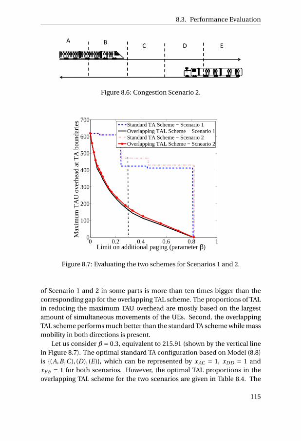
8.3. Performance Evaluation
Figure 8.6: Congestion Scenario 2.
0 0.2 0.4 0.6 0.8 10
100
200
300
400
500
600
700
Limit on additional paging (parameter β)
Max
imum
TA
U o
verh
ead
at T
A b
ound
arie
s
Standard TA Scheme − Scenario 1Overlapping TAL Scheme − Scenario 1Standard TA Scheme − Scenario 2Overlapping TAL Scheme − Scneario 2
Figure 8.7: Evaluating the two schemes for Scenarios 1 and 2.
of Scenario 1 and 2 in some parts is more than ten times bigger than thecorresponding gap for the overlapping TAL scheme. The proportions of TALin reducing the maximum TAU overhead are mostly based on the largestamount of simultaneous movements of the UEs. Second, the overlappingTAL scheme performs much better than the standard TA scheme while massmobility in both directions is present.
Let us consider β = 0.3, equivalent to 215.91 (shown by the vertical linein Figure 8.7). The optimal standard TA configuration based on Model (8.8)is {(A,B ,C ), (D), (E)}, which can be represented by xAC = 1, xDD = 1 andxEE = 1 for both scenarios. However, the optimal TAL proportions in theoverlapping TAL scheme for the two scenarios are given in Table 8.4. The
115

8. SIGNALING CONGESTION MITIGATION OF THE TRAIN SCENARIO
variables’ representations are based on the definition illustrated in Figure8.2. Variables not included in the table are zero.
Table 8.4: Optimal solutions for β= 0.3.
Scenario 1 Scenario 2STA OTAL STA OTAL
xA A 0 0.27 0 0.29xDD 1 0 1 0xEE 1 0.18 1 0.41xAB 0 0.26 0 0.24xAC 1 0.39 1 0.42xAD 0 0.08 0 0.05xBD 0 0.05 0 0.25xC D 0 0.26 0 0.11xC E 0 0 0 0.17xDE 0 0.60 0 0.37
The overhead results of these configurations are given in Tables 8.5 forthe two scenarios. As the TAL variables can take fractional values, the over-lapping TAL scheme is able to utilize all the possible total additional paging(TPAG) to the favor of reducing the maximum TAU (MTAU), i.e. T PAG =βC P for the overlapping TAL scheme in the table. The numerical resultsshow that the overlapping TAL scheme is able to mitigate the first conges-tion scenario by 61.49% and the second congestion scenario by 62.51% morethan the standard TA scheme for the limit under consideration, which isβ = 0.3. The fundamental flexibility of the overlapping TAL scheme in as-signing different proportions of each TAL significantly improves the perfor-mance compared to the standard TA scheme.
Table 8.5: Signaling overhead results for β= 0.3.
Scenario 1 Scenario 2STA OTAL STA OTAL
βC P 215.91 215.91 215.91 215.91MTAU 424.00 163.28 471.00 176.59TPAG 173.55 215.91 175.49 215.91
116

8.4. Conclusions
8.4 Conclusions
In this chapter, a low-complexity solution approach was presented basedon linear programming, to find the optimal proportional use of the lists ofTAs for the proposed overlapping TAL scheme. The congestion mitigationeffect was achieved by minimizing the maximum TAU signaling overheadin the network. The study showed that by assigning different TALs to theUEs involved in massive mobility, one can avoid the excessive TAU signalingmessages at the TA boundaries. The transitive property of the standard TAconfiguration is relaxed in the overlapping TAL scheme, which considerablyimproves the load balancing capability.
There are several topics deserving further research. One is to apply theoverlapping TAL scheme in a large-scale network to see its potentials com-pared to the standard TA scheme. This is studied in the following chapter.Another interesting subject worth studying is to extend the scheme by con-sidering more data in hand, for example assuming that the destination ofeach UE in a train is known.
117

CH
AP
TE
R
9SIGNALING CONGESTION MITIGATION
The rationale of avoiding signaling congestion is to ensure no significantdegradation in the quality of service, which may occur due to resource ex-haustion for tracking UEs. In addition to the train scenario explained in theprevious chapter, there are several types of mobility patterns that may causeTAU and paging congestion. As explained in Chapter 3, reconfiguring TAs inorder to adapt to the UEs movement behavior during peak hours typicallyrequires temporally turning down the cells, which is a costly process fromthe service perspective. This chapter aims to mitigate the signaling con-gestion resulted from mass mobility of idle UEs without performing a TArevision.
In previous studies of applying TALs, e.g., [35, 81, 118], the performancecomparison relies heavily on the assumptions made on UE mobility andother network parameters. Because UEs that are initially registered to thesame TAL by a cell will spread out within the area defined by the TAL, af-ter some time duration, as a result of each UE’s individual movement, theproportion of UEs assigned a certain TAL will become heterogeneous overthe area. Note that the amount of TAU and paging generated by a UE areboth dependent on the content of its TAL. Therefore, unless a very accuratemobility model is available (which is hardly the case in many scenarios), thepractical performance of TAL may deviate significantly from the estimatedone.
In the overlapping TAL scheme explained in the previous chapter, theconstruction of the LPs ensures the same proportional use of each TAL byall cells within the TAL. Therefore, statistically the proportion of UEs of eachTAL remains homogeneous with the TAL’s area, meaning that the perfor-mance is insensitive to individual UE movement. By assuming that the loca-
119

9. SIGNALING CONGESTION MITIGATION
tion distribution and mobility pattern of idle UEs are similar to those of ac-tive UEs, which is a well-accepted assumption, the performance of the over-lapping TAL scheme is conveniently assessed. This makes the performancecomparison both simple and unbiased, and its validity is not impacted bymobility models.
In this chapter, the LP formulation of the overlapping TAL scheme forthe train scenario is generalized to find the optimal proportional use of theoverlapping TALs for mitigating both TAU and paging congestions in large-scale networks. The study of this chapter has previously appeared in [86].
9.1 An Instructive Example
In this section, the overlapping TAL scheme for TAU congestion mitigationis explained using a small example of a network with four TAs in Figure 9.1.Each of these TAs contain multiple cells and the assumption is that the TAlayout in Figure 9.1 is optimum in terms of the total signaling overhead ofthe standard TA scheme. Suppose TALs which may partially overlap in theircomposition are created and assigned to UEs. Overall for the example inFigure 9.1, there are a total of fifteen TALs, each being a non-empty subsetof {1,2,3,4}.
Any UE in this network will be registered to one of these fifteen TALsand each TA belongs to its respective collections of TALs. For example, thecells in TA 1 potentially belong to eight TALs, which can be assigned to theUEs registered or updated in 1: {1}, {1,2}, {1,3}, {1,4}, {1,2,3}, {1,2,4}, {1,3,4},{1,2,3,4}. Each of these eight TALs has a proportional value of usage, andthe sum of all these values is one. For example TAL {1,3} can be assignedto a UE from cells of both TAs 1 and 3. If TAs 1 and 3 assign different pro-portional values of this TAL to their UEs, then the total number of UEs beingregistered to the TAL in the area of these two TAs will depend on the UEs mo-bility behaviors. It is assumed that, the two TAs apply the same proportionalvalues for the TALs containing both TAs. This assumption is generalized toany TAL, meaning that all TAs within the TAL are fully consistent in theirproportional use of the TAL.
To formalize the optimization framework, the proportional usage of TALℓ is denoted by a non-negative optimization variable xℓ. All cells in oneTA will apply the same collection of TALs, and they update their UEs withthe same proportional use of each TAL. For the network in Figure 9.1, thefour TAs apply their respective collections of TALs by Equations (9.1)-(9.4).Because the usage of any TAL ℓ is unified within the entire service area of ℓ,
120
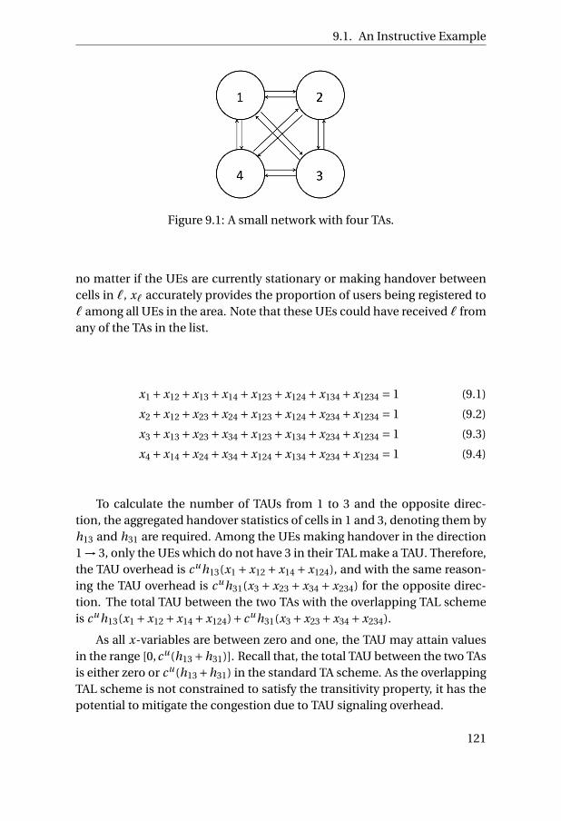
9.1. An Instructive Example
Figure 9.1: A small network with four TAs.
no matter if the UEs are currently stationary or making handover betweencells in ℓ, xℓ accurately provides the proportion of users being registered toℓ among all UEs in the area. Note that these UEs could have received ℓ fromany of the TAs in the list.
x1 +x12 +x13 + x14 +x123 +x124 +x134 +x1234 = 1 (9.1)
x2 +x12 +x23 + x24 +x123 +x124 +x234 +x1234 = 1 (9.2)
x3 +x13 +x23 + x34 +x123 +x134 +x234 +x1234 = 1 (9.3)
x4 +x14 +x24 + x34 +x124 +x134 +x234 +x1234 = 1 (9.4)
To calculate the number of TAUs from 1 to 3 and the opposite direc-tion, the aggregated handover statistics of cells in 1 and 3, denoting them byh13 and h31 are required. Among the UEs making handover in the direction1 → 3, only the UEs which do not have 3 in their TAL make a TAU. Therefore,the TAU overhead is cuh13(x1 + x12 + x14 + x124), and with the same reason-ing the TAU overhead is cuh31(x3 + x23 + x34 + x234) for the opposite direc-tion. The total TAU between the two TAs with the overlapping TAL schemeis cuh13(x1 +x12 +x14 +x124)+cuh31(x3 + x23 +x34 + x234).
As all x-variables are between zero and one, the TAU may attain valuesin the range [0,cu(h13 +h31)]. Recall that, the total TAU between the two TAsis either zero or cu(h13+h31) in the standard TA scheme. As the overlappingTAL scheme is not constrained to satisfy the transitivity property, it has thepotential to mitigate the congestion due to TAU signaling overhead.
121

9. SIGNALING CONGESTION MITIGATION
9.2 Congestion Mitigation of TAU
In this section, the optimization approach which was previously used forTAU congestion mitigation of the train scenario is generalized by optimizingthe TALs for a network region where massive TAU is of concern.
All cells in one TA will use the same collection of TALs, and they updatetheir UEs with the same proportional use of each TAL. The standard TA de-sign is considered as the underlying structure. For the network region inquestion, denote the current TAs forming the region by set T = {1, . . . ,T }.Each TA v ∈ T is a set of cells. The TAs can be, for example, optimized forthe total TAU and paging overhead.
A min-max approach for TAU congestion mitigation is applied, that is,TALs are used to minimize the maximum TAU between all pairs of TAs. Tothis end, an upper bound on the increase of the total paging overhead isnecessary, as otherwise the optimum would be to completely eliminate TAUby exclusively using the TAL containing all TAs. The bound is expressed asβC P , where C P is the total paging overhead of TA design T , and β is a non-negative parameter denoting the allowed percentage of increase.
The set of all possible TALs of T is denoted by L . Thus L is the set ofall non-empty subsets of T . The total load parameter of all cells inside TAv ∈ T is given by uv , and hv w denotes the total handover between TAs vand w . These values are easily derived from the load and handover valuesbetween cells. Parameter avℓ is a binary indicator, denoting whether or notTA v is in TAL ℓ. Moreover, nv denotes the number of cells in TA v . Theaforementioned continuous variable xℓ represents the proportional use ofTAL ℓ by all cells of the TAs in ℓ. An auxiliary variable z is used to denote themaximum TAU between TAs. The min-max TAU optimization problem canthen be modeled by the following LP.
min z (9.5a)
s. t.∑ℓ∈L
avℓxℓ = 1, v ∈T (9.5b)
cu(hv w∑ℓ∈L
avℓ(1−awℓ)xℓ+hw v∑ℓ∈L
awℓ(1−avℓ)xℓ) ≤ z, v, w ∈T , v = w
(9.5c)
αcp∑ℓ∈L
∑v∈ℓ
∑w∈ℓ,v =w
uv nw xℓ ≤βC P , (9.5d)
xℓ ≥ 0, ℓ ∈L . (9.5e)
The first constraint set (9.5b) assures that, within any TA, the propor-
122

9.3. Congestion Mitigation of Paging
tional usage values of TALs containing the TA sum up to one. This is thegeneralization of (9.1)-(9.4). The next set of constraints (9.5c) defines themaximum TAU between TA pairs. For each ordered pair v and w , there isa contribution of cuhv w xℓ, if TAL ℓ contains v (i.e., avℓ = 1) but not w (i.e.,awℓ = 0). Constraints (9.5d) bound the total paging overhead. For any list ℓ,the overhead imposed by paging UEs in TA v ∈ ℓ to TA w ∈ ℓ is αcp uv , scaledby the number of cells in w and variable xℓ that stands for the proportionaluse of ℓ.
It is often the fact that at the optimum of (9.5) the x-variables are frac-tional. As a result, some but not all of the UEs moving from one TA to an-other generate TAUs, in contrast to the original TA layout. In other words,the sharp boundaries between the TAs are “blurred” by the fractional use ofTALs.
The number of variables in (9.5) is exponential in the number of TAs T .However, in practice this is not problematic for two reasons. First, the regionwith high risk of excessive TAU is typically confined to a part of the network.Second, as (9.5) is an LP, it can be solved efficiently even for a large numberof variables.
9.3 Congestion Mitigation of Paging
The min-max optimization approach is not limited to congestion mitigationof TAU. It is easily adapted to reducing the risk of signaling congestion inpaging that may become of concern for scenarios where massive UEs arepopulated densely in some area with little mobility (e.g., a football stadium).The paging overhead in this area becomes considerably higher than that inthe rest of the network.
To reduce the paging overhead, some type of area splitting needs to takeplace. However, if the area would be in one common TA, such a split wouldnot be possible without reconfiguring the TAs into smaller ones. For clarityof the discussion, every single cell is assumed to be a TA in the current con-figuration. The assumption does not impose excessive TAU, because the ef-fect of “TA” of any size equivalently can be achieved by using a TAL contain-ing the corresponding single-cell TAs [35, 82]. Thus, in this section, it is as-sumed that TALs are already in place in the current TA design, but the func-tion has been limited to forming TAs in a conventional sense. For mitigatingpaging congestion, new (and smaller) TALs are created within the originalones, and their proportional usage levels are determined by the min-maxoptimization.
123

9. SIGNALING CONGESTION MITIGATION
Let T = {1, . . . ,T } be the set of single-cell TAs in the TAL containing thearea with risk of paging congestion. As in the previous section, L is used todenote the non-empty collections of elements of T . The other variable andparameter definitions are reused as well. Note that within T , TAU is zero forthe mentioned configuration (single TAL containing all TAs of T ). Reducingpaging would lead to a positive amount of TAU, and the limit is denotedby CU
lim. The min-max LP formulation of paging congestion mitigation isprovided in (7.1).
min z (9.6a)
s. t.∑ℓ∈L
avℓxℓ = 1, v ∈T (9.6b)
αcp∑
v∈T
uv∑ℓ∈L
avℓawℓxℓ ≤ z, w ∈T (9.6c)∑v∈T
∑w∈T :v =w
cu(hv w∑ℓ∈L
avℓ(1−awℓ)xℓ+hw v∑ℓ∈L
awℓ(1−avℓ)xℓ) ≤CUlim,
(9.6d)
xℓ ≥ 0, ℓ ∈L . (9.6e)
The first set of constraints are identical to that of (9.5). Constraints (9.6c)define, together with the objective, the maximum paging. For each single-cell TA w , the left-hand side of (9.6c) represents the total amount of over-head generated to w because of paging UEs located in TAs other than w ,due to the use of TALs with multiple cells. The next constraint set is theaggregated form of (9.5c) to represent the total TAU, bounded by the limitvalue in the right-hand side.
The fixed limit value in (9.6) and parameter β in (9.5) are not necessarilyconsidered constants prior to running TAL optimization. In fact, the LP canbe solved repeatedly for a range of limit values. Doing so generates a setof candidate solutions representing various levels of the trade-off betweencongestion reduction of TAU and the price of more paging, and vice versa(cf. Pareto optimization).
9.4 Performance Evaluation
In the following performance evaluation, TA and TAL are defined on the sitelevel and the overhead of a single TAU, cu is set ten times as much as cp [66].Parameter α is set to 0.05, i.e. 5% of the UEs are paged. Table 9.1 gives thenumerical assumptions and values for this performance evaluation.
124
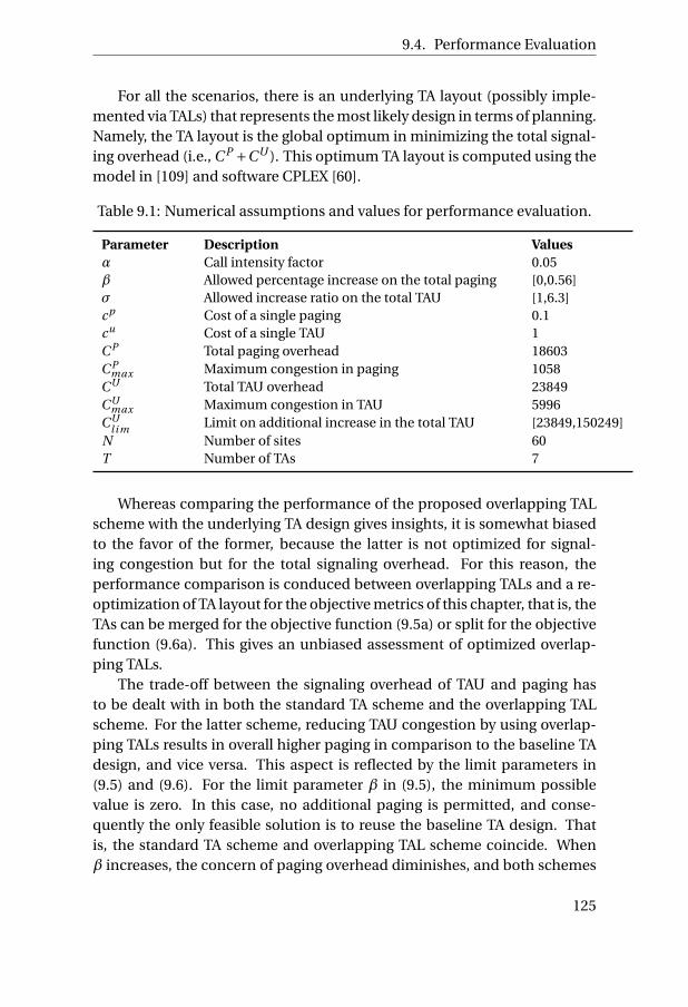
9.4. Performance Evaluation
For all the scenarios, there is an underlying TA layout (possibly imple-mented via TALs) that represents the most likely design in terms of planning.Namely, the TA layout is the global optimum in minimizing the total signal-ing overhead (i.e., C P +CU ). This optimum TA layout is computed using themodel in [109] and software CPLEX [60].
Table 9.1: Numerical assumptions and values for performance evaluation.
Parameter Description Valuesα Call intensity factor 0.05β Allowed percentage increase on the total paging [0,0.56]σ Allowed increase ratio on the total TAU [1,6.3]cp Cost of a single paging 0.1cu Cost of a single TAU 1C P Total paging overhead 18603C P
max Maximum congestion in paging 1058CU Total TAU overhead 23849CU
max Maximum congestion in TAU 5996CU
li m Limit on additional increase in the total TAU [23849,150249]N Number of sites 60T Number of TAs 7
Whereas comparing the performance of the proposed overlapping TALscheme with the underlying TA design gives insights, it is somewhat biasedto the favor of the former, because the latter is not optimized for signal-ing congestion but for the total signaling overhead. For this reason, theperformance comparison is conduced between overlapping TALs and a re-optimization of TA layout for the objective metrics of this chapter, that is, theTAs can be merged for the objective function (9.5a) or split for the objectivefunction (9.6a). This gives an unbiased assessment of optimized overlap-ping TALs.
The trade-off between the signaling overhead of TAU and paging hasto be dealt with in both the standard TA scheme and the overlapping TALscheme. For the latter scheme, reducing TAU congestion by using overlap-ping TALs results in overall higher paging in comparison to the baseline TAdesign, and vice versa. This aspect is reflected by the limit parameters in(9.5) and (9.6). For the limit parameter β in (9.5), the minimum possiblevalue is zero. In this case, no additional paging is permitted, and conse-quently the only feasible solution is to reuse the baseline TA design. Thatis, the standard TA scheme and overlapping TAL scheme coincide. Whenβ increases, the concern of paging overhead diminishes, and both schemes
125

9. SIGNALING CONGESTION MITIGATION
eventually coincide again, giving the same solution with one single TA (orTAL) containing all sites with zero TAU overhead. At this point, constraint(9.5d) is void, and increasing β further clearly has no effect. A similar obser-vation applies to the TAU limit in (9.6). Namely, the two schemes coincidewhen the limit is zero for which the baseline TA design is kept, or when thelimit is very large such that the optimum for both is to split TAs maximallywith zero paging (but completely sacrifices TAU). Thus, for each of the limitparameters, there is a maximum value of significance.
In the performance evaluation, for each limit parameter, its maximumvalue of significance is found by using bi-section search for the given plan-ning scenario. Then, within the range of significance, computations for 500equally-spaced values of the limit parameter are conducted, in order to givea comprehensive performance picture. The results represent, in fact, a largenumber of possible options for the trade-off between TAU and paging, bothfor the standard TA scheme and for the overlapping TAL scheme, allowingthe network operator to select the solution to implement, based on the op-erator’s preference.
The data from the Lisbon network is again used for performance evalua-tion on a general and large-scale topology. Figure 9.2 illustrates the underly-ing TA layout (i.e., the optimum with respect to the total signaling overhead).There are seven TAs in the design; these are used for creating overlappingTALs. Note that, in mitigating signaling congestion of paging, the function-ality of the standard TA scheme is implemented with non-overlapping TALsof single-sited TAs (see Section 9.3). In this case, the term TA group is usedfor the sake of clarity.
Key statistics of the TA design are as follows. The total TAU overhead isCU = 23849, and the total paging overhead is C P = 18603. The highest TAUbetween TAs, denoted by CU
max = 5996, and the most congested site in paginghas a paging overhead of C P
max = 1058.
For parameter β, the range of significance in this case is [0,0.56]. For-mulation (9.5) in Section 9.2 is solved with β varying within the range. Thesame range is applied in re-optimizing TAs with the standard TA scheme forthe same objective function (9.5a). The results are displayed in Figure 9.3and Table 9.2. In addition to the signaling overhead, the table contains in-formation of the computing time.
As was previously explained in Chapter 8 for the case of train scenario,the performance curves coincide at the two ends. One immediate obser-vation is that the curve of the overlapping TAL scheme is smooth, whereasthat of the standard TA scheme has a stepwise shape. For the latter, the TAs
126

9.4. Performance Evaluation
Figure 9.2: The underlying TA design.
Table 9.2: Performance comparison for TAU congestion mitigation.
β Standard TA scheme Overlapping TAL schemeMaximum TAU Time (ms) Maximum TAU Time (ms)
0.0 5963 - 5953 80.1 4109 52 537 120.2 2953 52 131 120.3 2423 76 62 120.4 1910 60 37 120.5 373 230 14 12
127

9. SIGNALING CONGESTION MITIGATION
Figure 9.3: Evaluating the TAU congestion mitigation.
may not overlap due to the binary and transitive properties of the S(t) ma-trix (Section 5.1). As a result, the only possibility of reducing the maximumTAU is by merging TAs. This inherent limitation of the standard TA schemeleads to the stepwise shape. Overlapping TALs, in contrast, can achieve “par-tial merge” of TAs, by solving the optimization formulation (9.5), yielding asmooth curve that significantly outperforms the standard TA scheme.
For example, if the total paging overhead is allowed to increase by 10%,re-optimizing TAs by the standard TA scheme reduces the peak TAU be-tween TAs from CU
max = 5996 to slightly above 4109. Using optimized over-lapping TALs, the peak is pushed down to 537, see Table 9.2. This is onlyone seventh of the maximum TAU resulted from the standard TA scheme.Hence, TAU signaling congestion can be effectively handled by the proposedTAL scheme with little price paid for a higher amount of paging.
Examining the computing time in Table 9.2 shows that solving (9.5) forTAU mitigation runs very fast, and the computing time is not sensitive at allto the limit value. In fact, the overlapping TAL scheme runs several timesfaster than the standard TA scheme. In conclusion, the former has superiorperformance both in TAU mitigation and the computational burden.
Figures 9.4 and 9.5 provide illustrations of the designs corresponding to
128

9.4. Performance Evaluation
Figure 9.4: The standard TA design for a chosen maximum TAU.
the two markers in Figure 9.3. The standard TA scheme and overlappingTAL give the same level of peak TAU (approximately 2400) for the selectedsolutions, although the former has considerably higher paging. Figure 9.4shows the TA layout given by the standard TA scheme; one can see this lay-out is a simple merge of TAs 1-3 in Figure 9.2. The composition and usageof TALs are shown in Figure 9.5. In this figure, the original three TAs are stillused, but to lesser extent. In addition, TALs containing pairs of TAs are inplace, with the effect of reducing TAU peak between them. The illustrationhighlights the effect of blurring TA boundaries by overlapping TALs.
As the last part of the performance evaluation, the overlapping TAL schemeis applied for mitigating paging congestion, using Figure 9.2 as the base lay-
129

9. SIGNALING CONGESTION MITIGATION
Figure 9.5: The overlapping TAL design for a chosen maximum TAU.
Table 9.3: Performance comparison for paging congestion mitigation.
σ Standard TA scheme Overlapping TAL schemeMaximum paging Time (s) Maximum paging Time (s)
1.0 1058 - 1058 < 11.2 847 45 201 331.4 501 555 72 941.6 400 340 22 18811.8 340 517 11 2592.0 324 378 6 384
130

9.4. Performance Evaluation
1 2 3 4 5 6 70
200
400
600
800
1000
Limit of total TAU (parameter σ)
Max
imum
site
pag
ing
Standard TA SchemeOverlapping TAL Scheme
Figure 9.6: Evaluating the paging congestion mitigation.
out. In this case, the TAs are assumed to be single-sited, and the groupingin Figure 9.2 is implemented by means of non-overlapping TALs explainedin Section 9.3. Overlapping TALs are then created and optimized by formu-lation (9.6) to achieve partial split within each TA group. The TA groups arealso re-optimized following the standard principle of TA design; this cor-responds to finding the optimal split (with sharp boundaries) for objectivefunction (9.6a). The performance comparison is given in Figure 9.6 and Ta-ble 9.3. For the sake of compactness, the results represent the aggregatedvalues over all TA groups. Thus CU
lim can be set in relation to CU of the base-line design. The ratio between CU
lim and CU is denoted by σ. The range ofsignificance for the scenario is σ ∈ [1.0,6.3].
In the figure, the horizontal axis is σ, For example, σ = 2.0 on the axismeans that CU
lim = 2CU . The vertical axis represents the maximum pagingoverhead generated by the sites. For each site, this overhead is the amountof paging overhead of the site in order to locate UEs of other sites. When σ=1.0, the only feasible solution is to keep the baseline TA groups, for which themaximum site paging equals C P
max. The maximum decreases gradually inrespect of σ, and reaches zero (i.e., full split) when σ≥ 6.3. Note that in Table9.3, σ is limited to 2.0, because the maximum paging in the overlapping TAL
131

9. SIGNALING CONGESTION MITIGATION
scheme is virtually zero beyond this point.In comparison to Figure 9.3, the performance curve of the standard TA
scheme in Figure 9.6 is much smoother. This is because splitting a TA groupcan be done with a much better granularity (e.g., one site at a time) thanmerging TAs. Nevertheless, the performance is evidently inferior to that ofadopting overlapping TALs, as can be seen from Figure 9.6 and Table 9.3.The overlapping TAL scheme is able to reduce the maximum paging muchmore steeply in comparison to conventional split of TA groups. For example,the former virtually eliminates paging, if the TAU is allowed to be doubled(i.e., σ = 2.0), whereas in the latter case the maximum paging is still aboveone third of the baseline value, as shown in Table 9.3. Moreover, the mag-nitude of the performance difference grows in σ for the range consideredin the table. As another comparison, recall that the average site paging ofthe baseline design is approximately 310 (that is, C P divided by the num-ber of sites), and suppose it is of interest to bring the maximum paging leveldown to this value, for which the horizontal dashed line in the figure showthe performance of the two schemes. Using the standard TA scheme (orequivalently non-overlapping TALs), the TAU overhead has to be doubled.With optimized overlapping TALs, the effect is achieved with merely a 13%increase in TAU. Thus overlapping TALs provide an effective means of split-ting hotspots for avoiding paging congestion.
In Table 9.3, the computing time used by the overlapping TAL schemeis up to 30 minutes. The major part of the time is attributed to the largestTA group with 16 sites, see Figure 9.2. For this TA group, the LP (9.6) con-tains 216 −1 variables. Although the run time may not admit on-line use, itremains reasonable in a planning stage, because typically a hotspot of mas-sive and close-to-static UEs can be predicted in advance. It is also observ-able that time values for the overlapping TAL scheme and the standard TAscheme are comparable in magnitude, and the former scheme runs fasterfor all except for two cases in the table.
9.5 Conclusions
This chapter presented a scheme using a overlapping TALs and a min-maxoptimization approach for the purpose of mitigating signaling congestionfor location management in LTE networks. The optimization task was for-mulated and computed by means of linear programming. As the key aspectof the optimization framework, consistency in the proportional use of TALsis maintained throughout the network, and consequently no assumption
132

9.5. Conclusions
or model of UE mobility is required in order to assess the performance ofoverlapping TALs. Numerical evaluations of mitigating massive TAU as wellas paging congestion demonstrated that the proposed optimization frame-work is very effective. Optimization of overlapping TALs significantly out-performs the standard TA scheme in signaling congestion. By providinghigh granularity in re-distributing the signaling overhead over the networkarea, TALs open up a new dimension of freedom in location management.
An interesting line of extension of the current work is dynamic config-uration of overlapping TALs. By monitoring TAU and paging statistics andadapting the proportional use of TALs accordingly, the proposed TAL schemecan be extended to form an automated process in location managementwithin the paradigm of self-optimization networks. This topic will be ad-dressed in the next chapter.
133


CH
AP
TE
R
10STUDY OF STATIC AND DYNAMIC
DESIGNS
Conventionally, TAs are manually configured and the design is static. Whilenetwork conditions change, this approach is not efficient for reconfiguringTAs. The static design often does not perform very well in terms of the sig-naling overhead, but it has the advantage of low computational complexity.In contrast, a dynamic approach that frequently updates the designs mayachieve better results, while requiring a higher degree of computational ef-fort [39, 47].
Self-Organizing Networks (SON) capability is one of the key componentsof the LTE network. Automatic dynamic configuration is a key aspect forSON. Although the concept of automated reconfiguration is not new in cel-lular networks and there are already extensive uses of automated processesin performance engineering, introducing a higher level of automation re-mains one of the key topics in cellular communications. In Releases 8 and9, 3GPP is standardizing self-optimizing and self-organizing capabilities forLTE. This was a continuation of the natural evolution of automation in cel-lular networks by extending the scope deeper into the network for LTE [9].SON techniques aim at doing both planning and reconfiguration in a semi-autonomous fashion.
Due to the complexity of TA reconfiguration, until now the operatorsdecide about the TA of each cell at the time of network deployment, andchanges are made only in case of extreme performance degradations. Thenetwork continuously collects UE statistics and monitors performance in-dicators, and in SON there is a potential of improving the TA or TAL designsin short time intervals without any cost in terms of service interruption [97].
135

10. STUDY OF STATIC AND DYNAMIC DESIGNS
The aim of this chapter is to study the performance of the standard TAscheme under static and dynamic frameworks. The comparison of the twoframeworks helps in understanding the potential of SON in reducing theOPEX of the network. Moreover, the problem of signaling congestion mit-igation is studied in a dynamic framework. The dynamic framework is in-tended to correspond to SON mechanism. The work presented here haspartially been published in [82].
10.1 SON Dynamic Framework
In a dynamic framework, the optimum configuration is always based on thedata which has been collected until that specific point in time. However, theoptimum design based on the gathered data up till that time, may not re-main optimum for the next time interval. This is due to the dynamic changein UEs’ behaviors. Hence, the challenge in the dynamic framework study isthe signaling overhead estimation based on different sets of available data.
Previously in [82, 83], the challenge was tackled by defining differentsets of signaling overhead values including ideal, potential and actual. Theideal/potential signaling overhead represented the signaling overhead of ap-plying the STA/TAL design made for data of time interval d to the same data.The actual signaling overhead, which was the most practically feasible esti-mation among all, represents the signaling overhead of applying the designmade for data of time interval d −1 to the data of time interval d . However,in this case the design was optimized for one set of data and applied to thenext set of data, therefore the approach was vulnerable to consecutive setsof data, and may not be practical for SON. In this section, a mechanism touse the data collected from SON is proposed for the design of standard TAand TAL layout in a dynamic framework. A realistic assumption consideredin this study is that the similarity of data degrades by the increase of timeinterval.
The dynamic SON time framework is denoted by the set D = {1, . . . ,D},and D is the total number of data sets. The data entering the optimizationmodel ui (d) and hi j (d) are defined to be the weighted sum of the previousvalue and the new data gathered in the last time slot ui (d −1) and hi j (d −1).The idea is to smoothly reduce the impact of old data sets, and not makinga sharp change in the design of two consecutive time slots. With each col-lected data from SON, ui (d−1) and hi j (d−1), the new aggregated ui (d) andhi j (d) are computed by Equations (10.1) and (10.2). These two equationsare referred to as "exponential filters" in the glossary of statistical terms,
136

10.2. Congestion Mitigation in SON
where λ is a constant between 0 and 1 that smooths the changes in ui (d)and hi j (d).
ui (d) = (1−λ)ui (d −1)+λui (d −1) (10.1)
hi j (d) = (1−λ)hi j (d −1)+λhi j (d −1) (10.2)
The total TAU and paging signaling overhead for the TA design of timeslot d , Sd(t) are denoted by CU (d) and C P (d), respectively. Equations (10.3)and (10.4) compute the TAU and paging signaling overheads for each timeslot d . If cells i and j are in different TAs, according to Equation (10.3) themovement between the two cells contributes to CU (d). Based on Equation(10.4), the total paging overhead generated by cell i to other cells in the sameTA is computed by the load of cell i and the size of that TA. Note that a pagingoverhead is generated in each of the cells in the TA, except the cell where theUE is located. This is considered by the inner summation. By adding thepaging overhead of all cells in the network (the outer summation), the totalpaging overhead is calculated for time slot d .
CU (d) = ∑i∈N
∑j∈N : j =i
cuhi j (d)(1− sdi j (t)), d ∈D (10.3)
C P (d) = ∑i∈N
∑j∈N : j =i
αcp ui (d)sdi j (t), d ∈D (10.4)
10.2 Congestion Mitigation in SON
The SON mechanism can combine the static and dynamic framework basedon the network behavior. The TAU and paging congestion problems donot exist all the time, but only during certain time intervals and locations.Hence, the standard TA scheme can be kept until the time when TAU con-gestion reaches a certain threshold. According to the study in Chapter 9,the objective of the overlapping TAL scheme is to minimize the maximumTAU overhead between the TA boundaries or paging overhead of a standardTA scheme. Thus based on the SON mechanism, whenever the maximumTAU signaling at the TA borders exceeds a pre-defined threshold value, sayξ, the overlapping TAL scheme is applied to reduce this value and to avoidthe congestion in the network.
One major issue in applying the overlapping TAL scheme in a dynamicframework is making a reasonable assumption for the parameter β in (9.5)
137

10. STUDY OF STATIC AND DYNAMIC DESIGNS
and σ in (9.6). A relatively high value for β or σ can completely eliminate thecongestion problem, while it introduces a large amount of paging overheador TAU overhead in each time interval, whereas β or σ of very small sizemight not solve the problem of congestion to the limit lower than ξ. This infact opens a new problem which deserves further research.
An alternative in using the overlapping TAL scheme is the fact that theset T can denote the TAs inside the congested region and not the total TAsof the entire network. Therefore, one mechanism is that while MME mon-itors the TAU and paging overheads and determines the congestion area, itcan allow only those TAs with high TAU or paging at their boundaries andtheir neighboring TAs to enter the optimization formulations (9.5) or (9.6),respectively. In this way the problem significantly reduces in size. However,this study explores the bigger picture and considers the entering of all theTAs of the network inside the optimization model and solves the problem ofexponentially higher size. One main reason is that the congestion can hap-pen in several parts of the network at the same time interval and as TAs aregeographically connected to each other, solving the congestion problemsindividually for small subsets of TAs, may omit the optimum proportionaluse of TALs which could be found by solving the overall problem.
10.3 Performance Evaluation
The performance evaluation in this chapter consists of two parts. One is tocompare static and SON dynamic framework for the standard TA scheme.The other one is to apply the overlapping TAL scheme in a dynamic frame-work, and evaluate its performance. The overlapping TAL scheme is studiedon the problem of TAU signaling congestion, because based on the availabledata, the TAU overhead contributed more in the total signaling overhead.However, it is expected that the mitigation of paging signaling congestionresults to a similar outcome.
In this study, the realistic data of the Lisbon network is again used, andthe performance evaluation has been applied at site level. The generatedtraffic data is simulated based on the mobility patterns of the city streets andthe traffic intensity of the region types (e.g. commercial, office, housing,...)differentiated at different times of the day and week. Due to a dynamicframework, for each time interval, there exists a set of site load and han-dover statistics, which are used as an approximation for idle UEs locationsand mobility behavior. The time frame of one entire week is considered inthe experiment and each time interval is one hour. Hence, the number of
138

10.3. Performance Evaluation
4.855 4.86 4.865 4.87 4.875 4.88 4.885 4.89 4.895 4.9
x 105
4.284
4.2845
4.285
4.2855
4.286
4.2865
4.287
4.2875
4.288
4.2885
4.289x 10
6(m)
(m)
Figure 10.1: An illustration of the number of mobility in the Lisbon networkon a Monday dawn (3:00-4:00).
data sets D is 168. The traffic is simulated to vary over different times ofeach day and different days of the week. This is especially observable whencomparing the weekdays to weekends. The UEs’ activities are very low dur-ing nights and higher during days with two peaks at the beginning and theend of the office hours. For example, Figure 10.1 illustrates a low number ofmobility between (3:00-4:00) of a Monday morning, and Figure 10.2 shows ahigh number of mobility at (17:00-18:00) of a Friday afternoon in the Lisbonnetwork.
139

10. STUDY OF STATIC AND DYNAMIC DESIGNS
4.855 4.86 4.865 4.87 4.875 4.88 4.885 4.89 4.895 4.9
x 105
4.284
4.2845
4.285
4.2855
4.286
4.2865
4.287
4.2875
4.288
4.2885
4.289x 10
6 (m)
(m)
Figure 10.2: An illustration of the number of mobility in the Lisbon networkon a Friday evening (17:00-18:00).
10.3.1 A Comparison of the Static and SON Dynamic STA
In the static TA, which is still the location management deployment in mostcellular networks, a standard TA design based on the average data of siteload and handover of the entire time period (in this case study: one week) isapplied to all the data sets. The optimum standard TA design is computedby CPLEX [60] using the model in [109].
The dashed lines in Figures 10.3 and 10.4 illustrate the total and the TAUsignaling overhead of the static standard TA scheme during the examinedweek. The values presented on the y-axis of all the forthcoming diagramsare all based on the same cost unit, and due to having the same unit, they
140

10.3. Performance Evaluation
Mon Tue Wed Thu Fri Sat Sun Mon0
500
1 000
1 500
2 000
2 500
3 000
3 500
4 000
4 500T
otal
Sig
nalin
g O
verh
ead
SON STA SchemeStatic STA Scheme
Figure 10.3: The total signaling overhead of the static and SON standard TAschemes.
are comparable. In the entire experiment, the call intensity factor α is setto 0.05, and the overhead of a single TAU cu is set ten times as much as cp
[66]. Table 10.1 summarizes all the numerical assumptions and values con-sidered in the following performance evaluation study.
Table 10.1: Numerical assumptions and values for performance evaluation.
Parameter Description Valuesα Call intensity factor 0.05β Allowed percentage increase on the total paging [0.05,0.1]λ Smoothing factor 0.75ξ Paging threshold value 100cp Cost of a single paging 0.1cu Cost of a single TAU 1D Number of data sets 168N Number of sites 60T Number of TAs [11 - 30]
To apply SON on the standard TA scheme, the data is calculated accord-ing to the exponential filters explained in Section 10.1. This data is used forthe standard TA design of each time interval. However in SON, the TA layoutis applied to the network’s data of the next time interval. This assumption
141

10. STUDY OF STATIC AND DYNAMIC DESIGNS
Mon Tue Wed Thu Fri Sat Sun Mon0
500
1 000
1 500
2 000
2 500
3 000
3 500
4 000
4 500T
AU
Sig
nalin
g O
verh
ead
SON STA SchemeStatic STA Scheme
Figure 10.4: The TAU signaling overhead of the static and SON standard TAschemes.
has been previously explained in Section 10.1, and it is because in realitythere is no possibility of going back in time and applying the optimum de-sign to the same set of data. Note that the optimum design based on thehistory of UEs’ behaviors might not perform well for the next time interval.The λ value in this study is set to 0.75, this means that the current time in-terval has three times more impact than the aggregated data of the previoustime intervals. Larger values of λ actually reduce the level of smoothing, andin case of λ= 1 the data applied is just the same as the original data ui (d−1)and hi j (d − 1) for calculating the actual signaling overhead. While valuesof λ closer to zero have a greater smoothing effect and are less responsiveto recent changes. The solid lines in Figures 10.3 and 10.4 illustrate the to-tal and TAU signaling overhead of the SON standard TA scheme during theexamined week.
Figure 10.3 compares the total signaling overhead of the static and SONstandard TA scheme during the examined week. The key statistics of theTA design are as follows. There are 26 TAs in the static design, whereas inthe SON designs the number of TAs in different time intervals varies from aminimum value of 11 to a maximum of 30. The total signaling overhead ofthe static design during one week is
∑Dd=1(CU
st ati c (d)+C Pst ati c (d)) = 2.6304×
105, while in SON it has a 35.9% lower value,∑D
d=1(CUSON (d)+C P
SON (d)) =
142

10.3. Performance Evaluation
Mon Tue Wed Thu Fri Sat Sun Mon0
100
200
300
400
500
600M
axim
um T
AU
ove
rhea
d at
TA
bou
ndar
ies
SON STA SchemeStatic STA Scheme
Figure 10.5: The maximum TAU signaling congestion of the static and SONstandard TA schemes.
1.6864× 10⁵. According to Figure 10.4 which compares the TAU overheadof the static and SON standard TA schemes during the examined week, itcan be concluded that the improved total signaling overhead of the dynamicSON framework over the static one is a result of TAU overhead improvement.The total TAU overhead of the week is
∑Dd=1 CU
st ati c (d) = 2.3283×10⁵ for thestatic TA, and
∑Dd=1 CU
SON (d) = 9.0235×10⁴ for SON, that is 61.24% reduction.
The next step is to evaluate the problem of TAU congestion while a stan-dard TA design based on the minimization of total signaling overhead is ap-plied to the network. For the same static and SON frameworks explainedabove, the maximum and average TAU overhead have been computed atTA boundaries of the standard TA design for each time interval. Figure 10.5presents the maximum value of TAU among all TA boundaries for both static(dashed line) and SON (solid line) frameworks. Although the figure showsthat the static framework has higher TAU congested TAs compared to SONin the whole time frame, the difference is more highlighted for two peaks inthe morning and afternoon of the working days.
Figure 10.6 provides an illustration of the average TAU overhead at TAboundaries for the two frameworks. This explains that the SON standard TAscheme outperforms the static TA mostly on reducing the average TAU over-head, however the problem of congested TAs still remains while compar-
143

10. STUDY OF STATIC AND DYNAMIC DESIGNS
Mon Tue Wed Thu Fri Sat Sun Mon0
50
100
150A
vera
ge T
AU
ove
rhea
d at
TA
bou
ndar
ies
SON STA SchemeStatic STA Scheme
Figure 10.6: The average TAU signaling congestion of the static and SONstandard TA schemes.
ing Figures 10.5 and 10.6. This motivates the idea of applying the proposedoverlapping TAL scheme of Chapter 9 in order to mitigate the congestionsituations.
10.3.2 Applying the Overlapping TAL for Congestion Mitigation
In this section, the aim is to mitigate the TAU congestion in the SON stan-dard TA scheme presented with solid line in Figure 10.5. This figure showsthat the problem of TAU congestion does not exist in all time intervals. Thethreshold value ξ= 100 is set, and hence the overlapping TAL scheme is onlyapplied to the data of time intervals in which the maximum TAU at the TAboundaries is higher than this threshold value.
Figure 10.7 compares the TAU congested scenario of the SON standardTA scheme with the uncongested scenario while the overlapping TAL schemeis applied to the network. For each time interval, it is assumed that β= 0.1 informulation (9.5), meaning that the model allows 10% increase in the totalpaging of each time interval in order to minimize the TAU congestion. Thehorizontal line at 100 shows which time intervals are congested, and hencethe optimization model is applied only to those time intervals. The figureshows that with β = 0.1 the maximum TAU remains well below the thresh-
144

10.3. Performance Evaluation
Mon Tue Wed Thu Fri Sat Sun Mon0
50
100
150
200
250
300
350M
axim
um T
AU
ove
rhea
d at
TA
bou
ndar
ies
SON STA SchemeSON Overlapping TAL Scheme
Figure 10.7: The TAU signaling congestion mitigation by the overlappingTAL scheme (β= 0.1).
Mon Tue Wed Thu Fri Sat Sun Mon0
20
40
60
80
100
Tot
al a
dditi
onal
pag
ing
SON Overlapping TAL Scheme
Figure 10.8: Total additional paging (β= 0.1).
old value ξ= 100.
The goal is to avoid any TAU congestion however this does not mean to
145

10. STUDY OF STATIC AND DYNAMIC DESIGNS
Mon Tue Wed Thu Fri Sat Sun Mon0
50
100
150
200
250
300
350M
axim
um T
AU
ove
rhea
d at
TA
bou
ndar
ies
SON STA SchemeSON Overlapping TAL Scheme
Figure 10.9: The TAU signaling congestion mitigation by the overlappingTAL scheme (β= 0.05).
reduce the TAU overhead as much as possible. Note that additional pagingoverhead is added in each time interval by introducing the overlapping TALscheme. Figure 10.8 illustrates the amount of additional paging for eachtime interval for avoiding congestion. The total additional paging for thewhole week is∑D
d=1 C Paddi ti onal (d) = 5.1947×10³ for β= 0.1.
In the final step of the performance evaluation, the value of β is re-duced to 0.05 in order to see if the overlapping TAL scheme is able to mit-igate the TAU congestion. Figure 10.9 compares the TAU congested sce-nario of SON standard TA scheme with the SON overlapping TAL schemewhile β = 0.05. The figure shows that the overlapping TAL scheme is ableto mitigate the TAU congestion problem in most of the time intervals, andfor the time intervals which still have congestion, the maximum TAU over-head at the boundaries has been significantly reduced. Figure 10.10 illus-trates that the total additional paging in the case where β = 0.05 is only∑D
d=1 C Paddi ti onal (d) = 2.5973×10³.
From the numerical results, it is concluded that the proposed overlap-ping TAL scheme is highly able to mitigate the TAU congestion in a SON dy-namic framework. To fully mitigate the TAU congestion problem while notadding extra additional paging, SON can dynamically change the value of β
146

10.4. Conclusions
Mon Tue Wed Thu Fri Sat Sun Mon0
20
40
60
80
100T
otal
add
ition
al p
agin
g
SON Overlapping TAL Scheme
Figure 10.10: Total additional paging (β= 0.05).
based on the amount of congestion in different time intervals. Nevertheless,the performance of a fixed β is evidently satisfactory.
10.4 Conclusions
In this chapter, an automated process was proposed in location manage-ment of LTE networks within the paradigm of self-organizing networks. Theperformance of the standard TA scheme was examined under time-vary datawithin the static and SON dynamic frameworks. The problem of mitigatingTAU signaling congestion was tackled in a dynamic framework by using theoverlapping TALs. The TAU and paging statistics have been monitored andthe proportional use of TALs were adapted based on a linear program op-timization formulation. Numerical evaluations for mitigating massive TAUdemonstrated that the proposed dynamic optimization framework is veryeffective. The study was limited in having the data of only one week, how-ever by introducing more history of network’s behavior, SON can signifi-cantly improve the network performance.
147


CH
AP
TE
R
11CONCLUSIONS AND FUTURE RESEARCH
The dissertation work has dealt with four main themes. The first theme(Chapters 3-4) was TA design re-optimization considering a cost budget,and finding the Pareto-optimal solutions for the trade-off between the sig-naling overhead and the reconfiguration cost. Although these problems werestudied in the TA context, the results can be generalized to the study ofLA and RA optimization. The second theme (Chapters 5-7) dealt with theTAL concept and its potentials compared to the standard TA scheme. Thereare still many open problems which require more investigation in the TALscheme. The dissertation gave insight into the performance of TAL. Thethird theme (Chapters 8-9) dealt with the signaling congestion mitigationproblem. The dissertation proposed an overlapping TAL scheme which solvesthe well-known train problem scenario, and can be generalized to mitigatethe TAU and paging congestion in general topology. The fourth theme wasthe dynamic framework explored in Chapter 10. LTE supports SON, whichis one of the visions in future network management. The dissertation ex-amined the standard TA and the overlapping TAL schemes under a dynamicevaluation framework, in order to investigate the aptness of the schemes forSON.
11.1 Conclusions
The work presented in the dissertation justifies the benefit of tracking areaplanning and optimization for improving the performance in cellular net-works. There are also some detailed conclusions from each specific themestudied in the dissertation.
149

11. CONCLUSIONS AND FUTURE RESEARCH
Once a TA design is in use, adopting a new solution of green-field op-timization does not typically pay off in real networks. The repeated localsearch algorithm which is developed to solve the re-optimization problemin this dissertation is able to approach high-quality solutions. The noveltyof the approach is the consideration of the reconfiguration-cost budget.
Before applying any reconfiguration, a decision maker can be providedby a set of Pareto-optimal solutions of potential trade-offs between the sig-naling overhead and the reconfiguration cost. The proposed integer pro-gramming model provides the exact Pareto-optimal solutions, and the sug-gested GA algorithm gives close to optimal solutions for large-scale net-works in short time.
The signaling overhead obtained from the TAL assigned by the presentedlocal-search algorithm is half of the signaling overhead resulted from thestandard TA scheme. The rule of thumb in the dissertation is a very simpleand quick approach for assigning a reasonably good TAL for a large-scalenetwork.
Even if each cell is allowed to have a set of TALs to assign to its UEs, theoptimum TAL solution based on minimizing the total signaling overhead isto consider only one TAL for each cell. This conclusion is obtained from theLP model, and justifies the previously studied approaches, such as the ruleof thumb.
The proposed overlapping TAL scheme is able to successfully mitigateboth TAU and paging signaling congestion. The scheme is invaluable due toits independence from each UE’s specific mobility behavior.
The SON dynamic framework is able to significantly improve the perfor-mance of the network, even if a standard TA scheme is applied. The over-lapping TAL scheme can be applied whenever a congestion scenario occurs.The study shows that the scheme is able to successfully mitigate the signal-ing congestion in a dynamic fashion.
11.2 Suggestions for Future Work
There are still many open problems in the study of TA management of cel-lular networks. Some related topics deserving further research are summa-rized below.
The re-optimization problem explored in the dissertation for the stan-dard TA scheme can be extended to the TAL scheme. Even though in theTAL scheme the problem of service interruption in reconfiguration is solved,from the network standpoint it is still more preferable to avoid major changes
150

11.2. Suggestions for Future Work
between two consecutive configurations. Hence, another extension is to in-troduce a "change" budget in reconfiguring the TAL. It is also of interest tostudy the proposed TAL schemes under the defined SON dynamic frame-work.
In the performance evaluation of the static and dynamic frameworks,the aggregated data is based on short and equal-length time intervals. Dueto the effort required for data collection, it is of relevance to evaluate thetotal signaling overheads which resulted from considering data with higherlevel of aggregation.
Additional experimental analysis on larger networks and various topolo-gies can give more insights into the performance of the proposed algorithms.Another topic is the investigation of alternative and better optimization al-gorithms, especially for the TAL scheme, of which one example can be toextend the idea of rule of thumb to neighbors other than the first-hop onesin order to overcome the existing limitation.
One of the main extension lines of this research is to build an LM frame-work based on the overlapping TAL scheme. The framework should be com-patible for both minimization of the total signaling overhead, and mitiga-tion of the signaling congestion depending on the priority of either problemin the network. Reasonable thresholds must be computed for triggering theoverlapping TAL assignments according to the two problems.
In order to offer wireless coverage in different environments, rangingfrom the open outdoors to office buildings and undergrounds, Heteroge-neous Networks (HetNets) are defined [40]. HetNets are a gradual evolu-tion of cellular topology that involve a mix of radio technologies and celltypes (femto, pico, micro, and macro) working together seamlessly. HetNetsconsist of several subsystems, where each subsystem uses different accesstechnologies and protocols [45]. Location management study of HetNets,in which LAs, RAs and TAs coexist, will introduce new research problems inthis area.
151


BIBLIOGRAPHY
[1] 3GPP. TS 23.002 – v9.1.0. Network architecture. 3G Release 9, 2009.
[2] 3GPP. TS 23.401 – v8.6.0. General Packet Radio Services (GPRS) en-hancements for Evolved Universal Terrestrial Radio Access Network (E-UTRAN) access. 3G Release 8, 2009.
[3] 3GPP. TR 23.880 – v0.1.0. Stage2 for registration in densely-populatedarea (RED). 3G Release 8, 2007.
[4] 3GPP. TS 23.882 – v1.9.0. System architecture evolution: Report ontechnical options and conclusions. 3G Release 7, 2007.
[5] 3GPP TS 24.301 – v12.1.0. Technical specification group core networkand terminals; Non-Access-Stratum (NAS) protocol for Evolved PacketSystem (EPS). 3G Release 12, 2013.
[6] 3GPP TS 32.500 – v8.0.0. Self organizing networks (SON): concepts andrequirements. 3G Release 8, 2008.
[7] 3GPP TS 36.300 – v8.0.0. Overall description; Stage 2. 3G Release 8,2008.
[8] 3GPP TS 36.304 – v8.0.0. User Equipment (UE) procedure in idle mode.3G Release 8, 2008.
[9] 3GPP TS 36.902. Evolved Universal Terrestrial Radio Access Network(E-UTRAN); Self-configuring and self-optimizing network (SON) usecases and solutions. 3G Release 9, 2009.
[10] 3G Americas. The benefits of SON in LTE. White Paper, 2009.
[11] E. H. L. Aarts and J. H. M. Korst. Simulated Annealing and BoltzmannMachines. Wiley, 1989.
[12] E. H. L. Aarts and J. K. Lenstra. Local Search in Combinatorial Opti-mization. Wiley, 1997.
[13] D. K. Agrafiotis. Multiobjective optimization of combinatorial libraries.IBM Journal of Research and Development, 2001.
153

BIBLIOGRAPHY
[14] N. Akkari, S. Tohme, and M. Doughan. Vertical-to-horizontal han-dovers: Architecture and mobility management. In Proc. of WirelessCommunications and Networking Conference (WCNC ’07), 2007.
[15] I. F. Akyildiz, J. S. M. Ho and Y. B. Lin. Movement-based location up-date and selective paging for PCS networks. ACM/IEEE Transactions onNetworking, 4: 629-638, 1996.
[16] I. F. Akyildiz, J. McNair, J. S. M. Ho, H. Uzunalioglu, and W. Wang. Mo-bility management in next generation wireless systems. Proceedings ofthe IEEE, 87(8): 1347-1384, 1999.
[17] S. Z. Ali. Design of location areas for cellular mobile radio networks. InProc. of IEEE Vehicular Technology Conference (VTC ’02), pp. 1106-1110,2002.
[18] S. Almeida-Luz, M. A. Vega-Rodrigeuz, J. A. Gomez-Pulido, and J.M. Sanchez-Perez. Applying different evolution to the reporting cellsproblem. In Proc. of IEEE International Multiconference on ComputerScience and Information Technology, pp. 65-71, 2008.
[19] X. An, F. Pianese, I. Widjaja, and U. G. Acer. DMME: Virtualizing LTEmobility management. In Proc. of 36th IEEE Conference on Local Com-puter Networks, pp. 528-536, 2011.
[20] V. Angelakis, D. Gundlegård, B. Rajna, C. Rydergren, K. Vrotsou, R.Carlsson, J. Forgeat, and et al. Mobility modeling for transport effi-ciency - Analysis of travel characteristics based on mobile phone data.In Proc. of Mobile Phone Data For Development (D4D ’13), 2013.
[21] C. Barnhart, E. L. Johnson, G. L. Nemhauser, M. W. P. Savelsbergh, andP. H. Vance. Branch-and-Price: Column generation for solving huge in-teger programs. Operations Research, 46(3): 316-329, 1998.
[22] A. Bar-Noy and I. Kessler. Tracking mobile users in wireless communi-cations networks. IEEE Transactions on Information Theory, 39: 1877-1886, 1993.
[23] A. Bar-Noy, I. Kessler, and M. Sidi. Mobile users: To update or not toupdate?. Wireless Networks, 2 :175-185, 1995.
154

Bibliography
[24] Y. Bejerano, M. A. Smith, J. Naor, and N. Immorlica. Efficient locationarea planning for personal communication systems. ACM/IEEE Trans-action on Networking, 14: 438-450, 2006.
[25] R. E. Bellman. Dynamic Programming. Princeton University Press,1957.
[26] D. Bertsimas and J. N. Tsitsiklis. Introduction to Linear Optimization.Athena Scientific, 1997.
[27] C. Bettstetter. Mobility modeling in wireless networks: Categorization,smooth movement, and border effects. ACM SIGMOBILE Mobile Com-puting and Communications Review, 5: 55-66, 2001.
[28] P. S. Bhattacharjee, D. Saha, A. Mukherjee, and M. Maitra. Location areaplanning for personal communication services networks. In Proc. of the2nd ACM International Workshop on Modeling, Analysis and Simula-tion of Wireless and Mobile Systems (MSWiM ’99), pp. 95-98, 1999.
[29] E. Cayirci and I. F. Akyildiz. Optimal location area design to minimizeregistration signaling traffic in wireless systems. IEEE Transactions onMobile Computing, 2: 76-85, 2003.
[30] M. Canales, J. R. Gallego, A. H. Solana, and A. Valdovinos. An adaptivelocation management scheme for mobile broadband cellular systems.In Proc. of the 6th International Symposium on Wireless Communica-tion Systems (ISWCS ’09), pp. 333-337, 2009.
[31] K. Chander, D. Juneja, S. Iyengar, and S. Mukhopadhyay. An agent-based smart solution for vertical handover in 4G. International Journalof Engineering Science and Technology, 2010.
[32] A. Charnes and W. W. Cooper. Goal programming and multiple objec-tive optimization, European Journal of Operational Research, 1: 39-45,1977.
[33] K. -H. Chiang and N. Shenoy. A 2-D random-walk mobility model forlocation-management studies in wireless networks. IEEE Transactionson Vehicular Technology, 53: 413-424, 2004.
[34] M. I. Chowdhury, M. Iqbal, N. Sultana, and F. Rahman. Analysing an an-alytical solution model for simulations mobility. International Journalof Wireless & Mobile Networks, 5: 111-124, 2013.
155

BIBLIOGRAPHY
[35] Y. W. Chung. Adaptive design of tracking area list in LTE. In Proc. of the8th IEEE International Conference on Wireless and Optical Communi-cations Networks (WOCN ’11), 2011.
[36] D. Chung, H. Choo and H. Y. Youn. Reduction of location update trafficusing virtual layer in PCS. In Proc. of the International Conference onParallel Processing (ICPP ’01), pp. 331-338, 2001.
[37] V. Chvatel. Linear Programming. Freeman, New York, 1983.
[38] W. J. Cook, W. H. Cunningham, W. R. Pulleyblank, and A. Schrijver.Combinatorial Optimization. Wiley, 1997.
[39] J. Cowling. Dynamic Location Management in Heterogeneous CellularNetworks, Thesis, University of Sydney, 2004.
[40] A. Damnjanovic, J. Montojo, Y. Wei, T. Ji, T. Luo, M. Vajapeyam, T. Yoo,O. Song, and D. Malladi. A survey on 3GPP heterogeneous networks.IEEE Wireless Communications, 18(3): 10-21, 2011.
[41] G. B. Dantzig. Linear Programming and Extensions. Princeton Univer-sity Press, 1963.
[42] I. Demirkol, C. Ersoy, M. U. Caglayan, and H. Delic. Location area plan-ning in cellular networks using simulated annealing. In Proc. of IEEEInternational Conference on Computer Communications (INFOCOM’01), pp. 13-20, 2001.
[43] I. Demirkol, C. Ersoy, M. U. Caglayan and H. Delic. Location area plan-ning and cell-to-switch assignment in cellular networks. IEEE Transac-tions on Wireless Communications, 3: 880-890, 2004.
[44] M. Ehrgott and X. Gandibleux (editors). Multiple Criteria Optimization:State of the Art Annotated Bibliographic Surveys. Kluwer Academic Pub-lishers, 2002.
[45] G. Fan, X. Lu, and S. Ci. Mobility Management in Heterogeneous Net-works, in Handbook of Computer Networks: LANs, MANs, WANs, the In-ternet, and Global, Cellular, and Wireless Networks. John Wiley & Sons,Inc., 2007.
[46] G. Fan, I. Stojmenovic, and J. Zhang. Elimination of generalized ping-pong effects using triple-layers of location areas in cellular networks.Computer Science and Information Systems, 5: 1-16, 2008.
156

Bibliography
[47] J. Ferragut and J. Mangues-Bafalluy. A self-organized tracking area listmechanism for large-scale networks of femtocells. In Proc. of Interna-tional Conference on Communications (ICC ’12), 2012.
[48] P. C. Fishburn. Lexicographic orders, utilities and decision rules: A sur-vey. Management Science, 20: 1442-1471, 1974.
[49] P. Garcia, V. Casares, and J. Mataix. Reducing location update and pag-ing costs in a PCS network. IEEE Transactions on Wireless Communica-tions, 1: 200-209, 2002.
[50] M. R. Garey and D. S. Johnson. Computers and Intractability: A Guideto the Theory of NP-Completeness. W. H. Freeman and Company, 1979.
[51] F. Glover. Tabu search - part 1. ORSA Journal on Computing, 1(2): 190-206, 1989.
[52] F. Glover. Tabu search - part 2. ORSA Journal on Computing, 2(1): 4-32,1990.
[53] F. Glover and M. Laguna. Tabu Search. Kluwer Academic Publishers,1997.
[54] D. E. Goldberg. Genetic Algorithms in Search, Optimization, and Ma-chine Learning. Addison-Welsey, 1989.
[55] P. R. L. Gondim. Genetic algorithms and location area partitioningproblem in cellular networks. In Proc. of IEEE Vehicular TechnologyConference (VTC ’96), pp. 1835-1838, 1996.
[56] Gurobi 3.0.1. Reference Manual. 2010.
[57] F. S. Hillier and G. J. Lieberman. Introduction to Mathematical Pro-gramming. McGraw-Hill, 1991.
[58] D. S. Hochbaum. Approximation Algorithms for NP-hard Problems.PWS Publishing, 1995.
[59] J. H. Holland. Adaptation in Natural and Artificial Systems. The Univer-sity of Michigan Press, Ann Arbor, 1975.
[60] ILOG CPLEX 10.0. User’s Manual. 2006.
157

BIBLIOGRAPHY
[61] H. Isermann. Proper efficiency and the linear vector maximum prob-lem. Operations Research, 22: 189-191, 1974.
[62] J. K. Karlof. Integer Programming: Theory and Practice. CRC Press, 2006.
[63] N. Karmarkar. A new polynomial time algorithm for linear program-ming. Combinatorica, 4(4): 373-395. 1984.
[64] J. K. Karlof, C. D. Gelatt, and M. P. Vecchi. Optimization by simulatedannealing. Science, 220(4598): 671-680, 1983.
[65] J. R. Koza. Survey of genetic algorithms and genetic programming. InProc. of WESCON ’95 - Conference Record: Microelectronics, Commu-nications Technology, Producing Quality Products, Mobile and PortablePower, Emerging Technologies, 1995.
[66] K. Kyamakya and K. Jobmann. Location management in cellular net-works: Classification of the most important paradigms, realistic sim-ulation framework, and relative performance analysis. IEEE Transac-tions on Vehicular Technology, 54: 687-708, 2005.
[67] A. H. Land and A. G. Doig. An automatic method for solving discreteprogramming problems. Econometrica, 28: 479-520, 1960.
[68] C. Y. Lee, S. J. Kim and T. Park. A design of multi-layered location reg-istration areas in micro-cellular systems, Telecommunication Systems,14: 107-120, 2000.
[69] B. Liang and Z. Haas. Predictive distance-based mobility managementfor PCS networks. In Proc. of IEEE Conference on Computer Communi-cations (INFOCOM ’99), pp. 1377-1384, 1999.
[70] Y. B. Lin. Reducing location update cost in a PCS network, IEEE Trans-actions on Networking, 5: 25-33, 1997.
[71] R. -H. Liou, Y. -B. Lin, and S. -C. Tsai. An investigation on LTE mobil-ity management. IEEE Transactions on Mobile Computing, 12: 166-175,2013.
[72] J. Lundgren, M. Rönnqvist, and P. Värbrand. Optimization. Studentlit-teratur, 2010.
158

Bibliography
[73] G. L. Lyberopoulos, J. G. Markoulidakis, D. V. Polymeros, D. F. Tsirkas,and E. D. Sykas. Intelligent paging strategies in future mobile telecom-munication networks, IEEE Transactions on Vehicular Technology, 44:534-554, 1995.
[74] T. Mach and R. Tafazolli. Mass mobility signaling congestion avoidancemechanism using randomized time distribution of cell reselections. InProc. of International Conference on Telecommunications (ICT ’09), pp.238-242, 2009.
[75] S. Martello and P. Toth. Knapsack Problems: Algorithms and ComputerImplementations. John Wiley & Sons, 1990.
[76] S. Mishra and O. K. Tonguz. Most recent interaction area and speed-based intelligent paging in PCS. In Proc. of IEEE Vehicular TechnologyConference (VTC ’97), pp. 505-509, 1997.
[77] J. E. Mitchell. Handbook of Applied Optimization. Oxford UniversityPress, 2002.
[78] Mitsubishi Electric. Tracking Areas Sizes and Tracking Area List Op-timization. Technical Report in 3GPP TSG RAN WG3 Meeting, R3-071931, 2007.
[79] S. Modarres Razavi and D. Yuan. Performance improvement of LTEtracking area design: a re-optimization approach. In Proc. of the 6thACM International Workshop on Mobility Management and WirelessAccess (MobiWac ’08), pp. 77-84, 2008.
[80] S. Modarres Razavi, D. Yuan, F. Gunnarsson, and J. Moe. Optimizingthe trade-off between signaling and reconfiguration: A novel bi-criteriasolution approach for revising tracking area design. In Proc. of IEEE Ve-hicular Technology Conference (VTC ’09), 2009.
[81] S. Modarres Razavi, D. Yuan, F. Gunnarsson, and J. Moe. Exploitingtracking area list for improving signaling overhead in LTE. In Proc. ofIEEE Vehicular Technology Conference (VTC ’10), 2010.
[82] S. Modarres Razavi, D. Yuan, F. Gunnarsson, and J. Moe. Dynamictracking area list configuration and performance evaluation in LTE. InProc. of Global Communications (GLOBECOM) Workshops, 2010.
159

BIBLIOGRAPHY
[83] S. Modarres Razavi. Tracking Area Planning in Cellular Networks, The-sis, Linköping University, 2011.
[84] S. Modarres Razavi and D. Yuan. Mitigating mobility signaling con-gestion in LTE by overlapping tracking area lists. In Proc. of the 14thACM International Conference on Modeling, Analysis and Simulationof Wireless and Mobile Systems (MSWiM ’11), pp. 285-292, 2011.
[85] S. Modarres Razavi, D. Yuan, F. Gunnarsson, and J. Moe. Perfor-mance and cost trade-off in tracking area reconfiguration: A Pareto-optimization approach. Journal of Computer Networks, 56: 157-168,2012.
[86] S. Modarres Razavi and D. Yuan. Mitigating signaling congestion inLTE location management by overlapping tracking area lists. Journalof Computer Communications, 35: 2227–2235, 2012.
[87] IST-2000-28088 MOMENTUM project. http://momentum.zib.de.
[88] Motorola. Long Term Evolution (LTE): A Technical Overview. TechnicalWhite Paper, 2007.
[89] Z. Naor and H. Levy. Minimizing the wireless cost of tracking mobileusers: an adaptive threshold scheme. In Proc. of IEEE InternationalConference on Computer Communications (INFOCOM ’98), pp. 720-729, 1998.
[90] G. L. Nemhauser and L. A. Wolsey. Integer and Combinatorial Opti-mization. Wiley, 1988.
[91] NEC. Tracking Area Concepts and Influence on Paging Load. TechnicalReport in 3GPP TSG RAN2 Meeting, R2-070655, 2007.
[92] C. H. Park and S. Soni. A simulated annealing based solution approachfor the two-layered location registration and paging areas partitioningproblem in cellular mobile networks. European Journal of OperationalResearch, 178: 579-594, 2007.
[93] K. E. Parsopoulos, D. K. Tasoulis, and M. N. Vrahatis. Multiobjective op-timization using parallel vector evaluated particle swarm optimization.In Proc. of IASTED International Conference on Artificial Intelligenceand Applications (AIA ’04), pp. 823-828, 2004.
160

Bibliography
[94] J. Plehn. The design of location areas in a GSM network. In Proc. of IEEEVehicular Technology Conference (VTC ’95), pp. 871-875, 1995.
[95] G. P. Pollini and C. L. I. A profile-based location strategy and its perfor-mance. IEEE Journal on Selected Areas in Communications. 15: 1415-1424, 1997.
[96] R. Prakash, Z. Haas, and M. Singhal. Load-balanced location manage-ment for cellular mobile systems using quorums and dynamic hashing.Wireless Networks, 7: 497-512, 2001.
[97] QUALCOMM Europe and T-Mobile. New SON User Case: Tracking AreaOptimization. Technical Report in 3GPP TSG RAN WG3 Meeting, R3-071594, 2007.
[98] C. R. Reeves and J. E. Rowe. Genetic Algorithms, Principles and Perspec-tives: A Guide to GA Theory. Kluwer, 2002.
[99] C. Rose and R. Yates. Minimizing the average cost of paging under delayconstraints. Wireless Networks, 1: 211-219, 1995.
[100] D. Saha, P. S. Bhattacharjee, and A. Mukherjee. Time efficient heuris-tics for cell-to-switch assignment in quasi-static/dynamic locationarea planning of mobile cellular network. Computer Communications,30: 326-340, 2007.
[101] S. K. Sen, A. Bhattacharya, and S. K. Das. A selective location updatestrategy for PCS users. Wireless Networks, 5: 313-326, 1999.
[102] I. Shayea, M. Ismail, and R. Nordin. Advanced handover techniquesin LTE-advanced system. In Proc. of International Conference on Com-puter and Communication Engineering (ICCCE ’12), 2012.
[103] G. Sierksma. Integer and Linear Programming: Theory and Practice.Marcel Dekker, 1996.
[104] R. E. Steuer. Multiple Criteria Optimization: Theory, Computation,and Application. John Wiley & Sons, 1986.
[105] R. E. Steuer, L. R. Gardiner, and J. Gray. A bibliographic survey of theactivities and international nature of multiple criteria decision making.Journal of Multi-Criteria Decision Analysis, 5: 195-217, 1996.
161

BIBLIOGRAPHY
[106] S. Subramaniam and G. Krishnamurthi. Load balancing locationmanagement. In Proc. of IEEE International Conference on Communi-cations (ICC ’01), pp. 2835-2839, 2001.
[107] S. Tabbane. An alternative strategy for location tracking. IEEE Journalon Selected Areas in Communications, 13: 880-892, 1995.
[108] E. G. Talbi. Metaheuristics: From Design to Implementation. John Wi-ley & Sons, 2009.
[109] D. W. Tcha, T. J. Choi, and Y. S. Myung. Location-area partition in acellular radio network. Journal of the Operational Research Society, 48:1076-1081, 1997.
[110] Telecom Cloud. LTE TA planning, 31. 11/100 56-HSC 105 50/1 Uen B,2009.
[111] G. Wan and E. Lin. A dynamic paging scheme for wireless commu-nication systems. In Proc. of the 3rd ACM International Conference onMobile Computing and Networking (MobiCom ’97), pp. 195-203, 1997.
[112] W. Wang, I. F. Akyildiz, G. L. Stüber, and B. Chung. Effective pag-ing schemes with delay bound as QoS constraints in wireless systems.Wireless Networks, 7: 455-466, 2001.
[113] W. L. Winston and M. Venkataramanan. Introduction to MathematicalProgramming. Brooks/Cole - Thomson Learning, 2003.
[114] T. Winter. Mobility management and network design for UMTS. InProc. of IEEE International Symposium on Personal, Indoor and MobileRadio Communications (PIMRC ’04), 2004.
[115] L. A. Wolsey. Integer Programming. Wiley, 1998.
[116] V. W. -S. Wong and V. C. M. Leung. Location management for next gen-eration personal communication networks. IEEE Network, 14: 18-24,2000.
[117] V. W. -S. Wong and V. C. M. Leung. An adaptive distance-based loca-tion update algorithm for PCS networks. In Proc. of IEEE InternationalConference on Communications (ICC ’01), pp. 2001-2005, 2001.
162
Bibliography
[118] Y. Zhang and M. Fujise. Location management congestion problem inwireless networks. IEEE Transactions on Vehicular Technology, 56: 942-954, 2007.
[119] K. Zhu, D. Niyato, P. Wang, E. Hossain, and D. I. Kin. Mobility andhandoff management in vehicular networks: A survey. Wireless Com-munications and Mobile Computing, 11(4): 459-476, 2011.
[120] E. Zitzler and S. Kunzli. Indicator-based selection in multi-objectivesearch. In Proc. of the 8th International Conference on Parallel Solvingfrom Nature (PPSN ’04), pp. 832-842, 2004.
[121] ZTE. Self Optimization for Tracking Areas, Technical Report in 3GPPTSG RAN WG3 Meeting, R3-071415, 2007.
163


AP
PE
ND
IX
AMATHEMATICAL MODELS NOTATION
Parameters
α Call intensity factor (probability that a UE has to be paged)β Allowed percentage increase on the total pagingγ Probability factor of UEs entering cell i and have been a TAL
in Qi
δ Probability factor of UEs in cell i assigned to a TAL differentfrom the one assigned by i
λ Smoothing factorξ Paging threshold valueσ Allowed percentage increase on the total TAUτ The time intervalaiℓ Binary indicator that identifies if cell i is in TAL ℓ
avℓ Binary indicator that identifies if TA v is in TAL ℓ
cp The overhead of a single pagingcpag i ng (i ) The total paging of cell icR (t) The total cost of reconfigurationcSO(t) The total signaling overhead of design tcT AU (i , j ) The total TAU overhead between i and jcu The overhead of a single TAUd(t,t0) Binary vector representing cells that have been assigned new TAshi j Number of UEs having handover from cell i to cell jn Number of items in the knapsack problemni length of a line segment starting with i in the train scenarionv Number of cells in TA v
165

A. MATHEMATICAL MODELS NOTATION
Parameters (cont.)
t Vector notation of cell-to-TA assignmentt0 The TA design currently deployedti The TA of cell iui Number of UEs in cell i scaled by the time proportion spent in cell ivi The value of item i in the knapsack problemwi The weight of item i in the knapsack problemz Maximum TAU at TA boundaries or paging in a congestion scenarioB The budget valueB ′ Total cell load factor corresponding to the budget levelC P Total paging signaling overheadC P (d) Total paging signaling overhead of the data set dC P
addi ti onal Total additional paging signaling overheadC P
M AX Maximum congestion in pagingCU Total TAU signaling overheadCU (d) Total TAU signaling overhead in the data set dCU
li m Limit on additional increase in TAUCU
M AX Maximum congestion in TAUD Number of data setsK Number of iterationLt al Length of the TALMT AU Maximum TAUN Number of cells/sitesNT AL Maximum number of TAs in TALPOPSIZE GA population sizePV The Preference Value of the designPV-MAX The threshold on PV valueS(t) Binary matrix presenting the TA configuration of all cellsT Number of TAsT PAG Total additional pagingW Maximum weight that knapsack can carryX t a
t al Percentage of UEs inside each t a having t al as their list.
Sets
D Set of all data in a dynamic frameworkL Set of all possible TALs of T
N Set of all cells/sitesQi Set of all neighbors of i having i in their TAL
166

Sets (cont.)
Qni Set of neighbors of n in Qi having both i and n in their TALsT Set of TAs currently in use
Variables
di (t , t 0) Binary variable that identifies if cell i has been assigned a new TAli j Binary variable that identifies if cell j is in the TAL of cell ipi t Binary variable that identifies if cell i belongs to TA tpi t 0 Binary variable that identifies if cell i belongs to the current TA t 0
si j (t) Binary variable that identifies if cell i and j are in the same TAsd
i j (t) Binary variable that identifies if cell i and j are in the same TA in the
data set dxi Binary variable that represents the knapsack problemxi j Continuous variable that represents the proportional use of TAL starting
from i to j in a train scenarioxiℓ Continuous variable that represents the proportional use of TAL ℓ by cell ixℓ Continuous variable that represents the proportional use of TAL ℓ by
all cells of the TAs in ℓ
167


AP
PE
ND
IX
BUE-TRACES SCENARIO
B.1 Generating UE-traces Scenario
Assuming that cell load, handover and the call intensity factor (α) are theavailable data of the UEs’ mobility behaviors of a network in order to gen-erate a reasonable UE-traces scenario, the following aspects should be con-sidered.
• The UE is more probable to exist in cells with higher cell load. Equa-tion (B.1), where ui is the load of cell i , estimates the probability ratioof cell i being the starting cell of a UE in the specified time period.
Pst ar t (i ) = ui∑j∈N u j
(B.1)
• The UE tends to move towards neighbors with high handover value.Equation (B.2) gives the probability of a UE moving from cell i to cellj , provided that the UE leaves cell i . The handover between i and j isdefined by hi j and the set of neighbors of cell i is denoted by Ai .
Pmove (i , j ) = hi j∑p∈Ai
hi p(B.2)
• Among the UEs inside the UE-traces scenario, α of them are paged inthe specified time period.
169
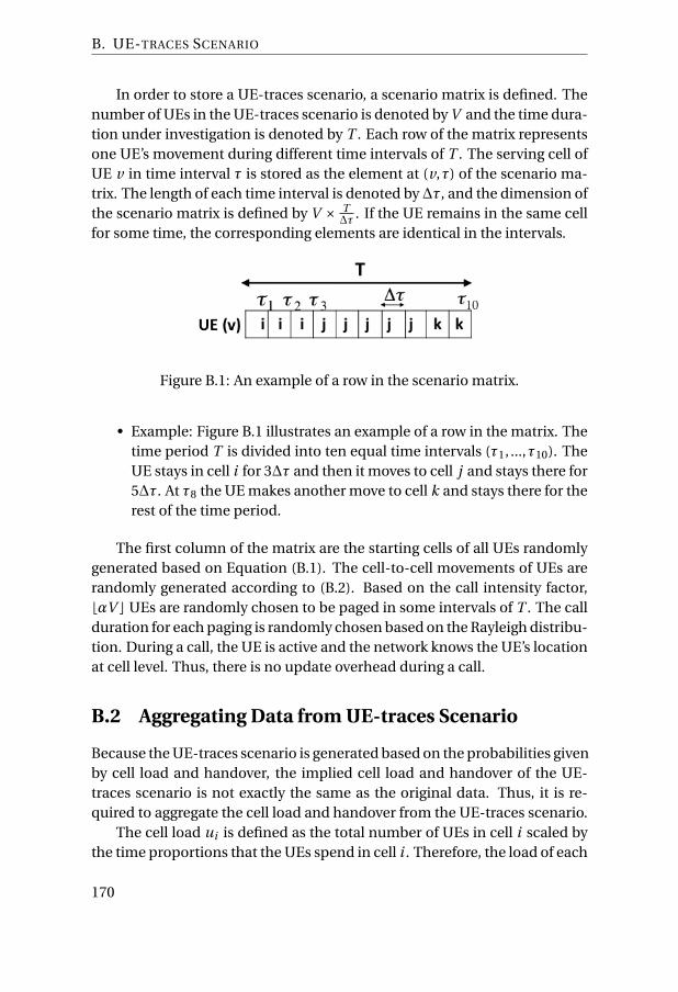
B. UE-TRACES SCENARIO
In order to store a UE-traces scenario, a scenario matrix is defined. Thenumber of UEs in the UE-traces scenario is denoted by V and the time dura-tion under investigation is denoted by T . Each row of the matrix representsone UE’s movement during different time intervals of T . The serving cell ofUE v in time interval τ is stored as the element at (v,τ) of the scenario ma-trix. The length of each time interval is denoted by ∆τ, and the dimension ofthe scenario matrix is defined by V × T
∆τ . If the UE remains in the same cellfor some time, the corresponding elements are identical in the intervals.
Figure B.1: An example of a row in the scenario matrix.
• Example: Figure B.1 illustrates an example of a row in the matrix. Thetime period T is divided into ten equal time intervals (τ1, ...,τ10). TheUE stays in cell i for 3∆τ and then it moves to cell j and stays there for5∆τ. At τ8 the UE makes another move to cell k and stays there for therest of the time period.
The first column of the matrix are the starting cells of all UEs randomlygenerated based on Equation (B.1). The cell-to-cell movements of UEs arerandomly generated according to (B.2). Based on the call intensity factor,⌊αV ⌋ UEs are randomly chosen to be paged in some intervals of T . The callduration for each paging is randomly chosen based on the Rayleigh distribu-tion. During a call, the UE is active and the network knows the UE’s locationat cell level. Thus, there is no update overhead during a call.
B.2 Aggregating Data from UE-traces Scenario
Because the UE-traces scenario is generated based on the probabilities givenby cell load and handover, the implied cell load and handover of the UE-traces scenario is not exactly the same as the original data. Thus, it is re-quired to aggregate the cell load and handover from the UE-traces scenario.
The cell load ui is defined as the total number of UEs in cell i scaled bythe time proportions that the UEs spend in cell i . Therefore, the load of each
170

B.2. Aggregating Data from UE-traces Scenario
cell in the network is aggregated by the scaled values of UEs staying in thecell using all the elements of the scenario matrix. The aggregated handovervalue is the number of moves from one cell to another.
• Example: Considering the example in Figure B.1 and that ∆τT = 0.1, the
aggregated cell load and handover from UE v are:
ui = 0.3, u j = 0.5, uk = 0.2, hi j = 1, and h j k = 1.
171
