Economics & Management Series EMS-2012-15

Planning under Correlated and Truncated Price andDemand Uncertainties

Wenkai LiInternational University of Japan

I. A. KarimiNational University of Singapore

R. SrinivasanNational University of Singapore

September 2012

IUJ Research InstituteInternational University of Japan

These working papers are preliminary research documents published by the IUJ research institute. To facilitate prompt distribution, they havenot been formally reviewed and edited. They are circulated in order to stimulate discussion and critical comment and may be revised. The viewsand interpretations expressed in these papers are those of the author(s). It is expected that the working papers will be published in some otherform.

1

Planning under Correlated and Truncated Price and Demand Uncertainties

Wenkai Lia,b

, I. A. Karimi*,b

, R. Srinivasanb

aGraduate School of International Management, International University of Japan, Niigata

949-7277, Japan bDepartment of chemical and Biomolecular Engineering, National University of Singapore, 4

Engineering Drive 4, Singapore 117576

ABSTRACT

This paper presents a novel approach to handle refinery planning under correlated and truncated random demand

and price uncertainties. To compute the expectation of plant revenue, which is the main difficulty for a planning

problem under uncertainty, a bivariate normal distribution is used to describe demand and price. Formulae for

revenue calculation under correlated and truncated price and demand are derived. It is found that the correlation

and truncation of price and demand have major influences on plant net profit. A plan that ignores these factors

can be far from optimal. The Type 2 service level or fill rate undercorrelated and truncated random price and

demand is derived and efficiently calculated in this paper. Maximum plant net profit that satisfies certain fill rate

target can thus be obtained. The proposed approach can be generally applied for modeling other chemical plants

under uncertainty.

Keywords: Refinery, Planning, Uncertainty, Correlation, Truncation

1. Introduction and motivation

Due to the changing market conditions, fluctuating environment and many other unobservable factors, many

parameters in an industry are uncertain. These uncertain parameters, such as fluctuating demands and volatile

raw material/product prices, are challenging and motivating decision makers to seek efficient managerial tools

and models to cope with the difficulty and achieve their KPIs. This ubiquitous phenomenon is thoroughly

exhibited in one of the most important industry in the national economy: the refining industry. The prices and

* Corresponding author. Email: cheiak@nus.edu.sg

2

demands of crude oil, gasoline and diesel oil are highly uncertain in reality arising from uncertain global and

national economic situations and indeterminate factors such as outbreaks of war, strikes and diseases, etc.

Uncertainty can be categorized into different types according to different criteria. From the time horizon point of

view, uncertainty can be categorized as short-term, mid-term and long-term uncertainty. Short-term uncertainty

includes day-to-day or week-to-week processing variations, canceled/rushed orders, equipment failure, etc.

Mid-term uncertainty addresses horizons of one to two years and incorporates some features from short-term

and long-term uncertainties1. Long-term uncertainty refers to raw material/final product unit price fluctuations,

demand variations, and production rate changes occurring over longer time frames ranging from five to ten

years.

From the process operation point of view, there are two types of uncertainties2: external uncertainties and

internal uncertainties. External uncertainties originate from outside but have impacts on the process. They can

be the feed rate and/or feed composition and recycle flows as well as flows of utilities, the temperature and

pressure of the coupled operating units or market conditions. Internal uncertainties come from the unavailability

of knowledge of the process. For a determined model structure, they are uncertain model parameters that are

often regressed from a limited number of experimental data. They can be the kinetic parameters of reactions in a

unit such as FCC (fluidized-bed catalytic cracker) or the transfer rate of a unit such as a CDU (crude distillation

unit).

From the observability point of view, uncertain parameters can be categorized into two types3: unknown

parameters and variable parameters. The exact values of unknown parameters are never known even though the

expected values may be known. These parameters include model parameters determined from experimental

studies such as the kinetic parameter of a reaction as well as unmeasured and unobservable disturbances such as

3

the influence of wind and sunshine. Variable parameters are not known at the design stage, but can be specified

or measured accurately at later operating stages. These include feed flow rates, product demands and process

conditions.

1.1. Correlation and truncation between uncertain demand and price

Among all the uncertainties discussed above, demand uncertainty has the dominant impact on plant profit and

customer satisfaction4,5

. Until now, most research work4,6

on uncertainty assumes that the demand and price are

independent and the price is assumed to be a constant because of the difficulty in computing the bivariate

integral originated from the correlated demand and price. Such methods are only as good as their underlying

assumptions. Furthermore, underlying the research of most previous papers4,6

, the ranges of demand and price

are assumed to be (– to +). This assumption may also bring significant inaccuracies in revenue calculation.

In this section, we show to what extent the real world demand and price are corrected and truncated.

1.1.1. Dependency between demand and price

Some researchers7 have studied the factors that influence the inter-correlation between demand and price. In

general, the main relationship between crude oil demand and price can be summarized in Figure 1. Many factors,

such as war, strikes, etc., influence the demand for crude oil. There are also many factors, such as the inventory

level, OPEC behavior, etc., influence the crude oil price. Crude oil demand has major influences on the price of

crude oil. However, this influence is weaker reversely. In both the long-run and short-run, the demand for crude

oil internationally is highly insensitive to changes in price8. By regressing real world demand and price data

from EIA (the U.S. Energy Information Administration)9, the correlation coefficient between gasoline (New

York Harbor Gasoline Regular) price and its demand is 0.44 for the year 2003 to 2004. For world crude oil in

2003 and 2004, the correlation coefficient is 0.30 (see Appendix I for regressing details). These data show that

4

the demand and price are far from independent. Some researchers4 have considered the correlation among

different products. However, no research work considers the correlation between demand and price so far.

Considering the correlation between the price and demand and studying its influences on plant revenue are the

main concern to be addressed in this paper.

Figure 1 Dependency between crude oil demand and price

1.1.2. Truncation of demand and price

Truncation can happen when a portion of data range is not attainable on physical grounds10

. An apparent

example is that the demand or price can only take positive values. In fact, despite their random nature, most real

world variables take values in a relatively narrow range. Table 1 lists some parameters estimated from the real

world demand and price data (EIA9). In the second row, the mean, and the standard deviation, , of the crude

oil demand in 2003–2004 are 49.2 and 1.3 million barrels/day, respectively. The maximum and minimum

demands in this period are 51.9 (=+2.1) and 47.2 (=–1.6) million barrels/day, respectively. Thus, we

obtain the range inside which crude oil demand locates in these two years: (). From the last

column of Table 1, it can be seen that, real world crude oil demand and price fluctuate one to two standard

deviations around their means.

Crude Oil

Demand

World Economy

Crude Oil

Price

War, Strikes…

Strong influence

Weak influence

Production Cost

Inventory level

Crude supply: OPEC behavior

5

Year / Max/Min Range:(-A*,+B*)

(A, B)

2003-2004

Total OECD crude oil demand*

Million barrels/day 49.2/1.3 51.9/47.2 (1.6, 2.1)

Crude Oil Price**

33.1/6.2 47.2/23.4 (1.6, 2.3)

1970-1999

World Total Oil Demand

Million barrels/day 65.3/8.6 82.6/46.8 (2.2, 2.0)

Crude Oil Price***

29.0/15.0 60.4/8.8 (1.3, 2.1)

*: Total OECD includes OECD Europe, Canada, Japan, South Korea, United States, and Other.

**: Brent, US$/barrel; ***: Venezuelan Tia Juana Light, US$/barrel (in 1999 real dollar)

Table 1 Ranges of the real world crude oil demand and price

Figure 2 shows the normally distributed truncated and non-truncated density functions. The difference between

the truncated and non-truncated density functions is obvious. Thus, using a non-truncated density function to

approximate a real world truncated density function may bring significant inaccuracies in revenue calculation

and a planning strategy based on this may far from optimal.

Non-truncated vs. Truncated Density Functions

0

0.01

0.02

0.03

0.04

-10 0 10 20 30 40 50 60

Non-truncated

Truncated

Figure 2 Normally distributed (=14.5) non-truncated and truncated (truncation range: –, + ) density

functions

Thomopoulos11

recognized that the impossibility of negative demands effectively truncates normally distributed

demand patterns. He used left-truncated normal distributions to determine safety stocks and shows how the

truncated normal distribution can be used to more accurately estimate the safety stock. Bookbinder and

Lordahl12

also used the left-truncated normal distribution to simulate the stochastic nature of demand patterns to

set the re-order point. Johnson A. et al.13

used univariate left-truncated normal distribution to improve the

achieved service level. They realized the significant computational errors in applications led by the

6

non-truncated normal distribution assumption. Johnson A. et al.14

extended the univariate left truncated normal

distribution to BLTN (bivariate left truncated normal distribution) and derived formula to approximate the

cumulative distribution function of BLTN. They then implemented the derived formula into EXCEL. However,

there exists an error in their extension which will be discussed later.

1.2. Solution approaches

Stochastic programming deals with problems in which some parameters incorporated into the objective or

constraints are uncertain. These uncertain parameters are usually described by probability distributions or by

possible scenarios in stochastic programming. Stochastic programming mainly consists of recourse models15

and

chance constrained programming4,6

, distinguished by the methods of describing uncertain parameters and the

algorithms of solving the model.

1.2.1. Recourse model and chance constrained programming

Recourse models use corrective actions (usually penalty functions) to compensate for the violation of constraints

arising during the realization of uncertainty. The two-stage model is one of the main paradigms of recourse

models. Two-stage model divides the decision variables into two stages. The first-stage variables are those that

have to be decided right now before future realization of uncertain parameters. Then, the second-stage variables

are those used as corrective measures or as recourse against any infeasibilities arising during the realization of

the uncertainty.

Because the exact values of the penalty terms are difficult to determine since they include intangible

components such as loss of goodwill, the costs of off-specification products or outsourcing of production

requirements in recourse models, in many cases of process operations, this penalty term is not available. This

7

difficulty is overcome in chance constrained programming. Chance constrained programming (or the

probabilistic approach) seeks to satisfy the constraints involved by a predetermined confidence level using the

known probability density/cumulative distribution of random variables16

. That is, rather than requiring

constraints containing the uncertain parameters always to be satisfied or imposing penalties for infeasibilities, a

probability of constraint satisfaction (usually called the confidence level) can be specified by the decision maker.

This approach provides comprehensive information on economic achievements as a function of the desired

confidence level.

Zimmermann17

argued that the choice of the appropriate method is context-dependent, with no single theory

being sufficient to model all kinds of uncertainty. A general-purpose algorithm is unlikely to solve all problems

efficiently or exactly. It might be a good strategy that one applies different approaches for different problems.

For design problems which penalty terms are easy to be obtained, using two-stage method is appropriate. For

problems that penalty terms are difficult to estimate, chance constrained programming is suitable. If the

computation speed is the main concern, fuzzy programming maybe a good choice. In this work, we extend the

approach presented in Li et al.6 for refinery planning under uncertainty to consider correlated and truncated

demand and price uncertainty. A bivariate normal distribution is used to describe demand and price. The double

integral for revenue calculation is reduced to several single integrals after detailed derivation. The unintegrable

standard normal cumulative distribution function in the single integrals is approximated by polynomial function.

1.2.2. Revenue calculation methods

The computation of the revenue of a plant involves uncertain variables such as market demand and product price.

How to compute the expectations of uncertain functions introduced by these uncertain variables generates the

main difficulty in stochastic rogramming18

and approaches in the literature differ primarily in how these

expectations are computed19

. Several approaches have been used in the literature to compute these expectations.

8

Clay et al.15

applied the certainty equivalent transformation (CET) to yield a deterministic equivalent problem.

Ierapetritou et al.20

used the Gaussian quadrature formula to approximate the expected revenue. Liu et al.21

used

Monte Carlo sampling to estimate the expectation of the objective function. Li et al.6 categorized different

revenue calculation approaches into three types which include: A) Minimizing cost. The objective is to

minimize the total costs and the computation of plant revenue is avoided. B). Maximizing profit I. The revenue

is calculated by the product of the market price and the amount of the product produced by the plant. In this

approach, it is assumed that a product can always be absorbed by the market. C). Maximizing profit II. The

revenue is calculated by the product of the market price and the market demand. In this approach, it is assumed

that the amount of a product is always greater than the market demand. However, the assumptions in B) and C)

are not always true in the real world. As pointed out by Petkov et al.4 and Li et al

6, in many cases, if the market

demand is less than the product amount, only part of the product can be sold; otherwise if the market demand is

higher than the product amount, then only part of the demand can be satisfied. The revenue should then be

calculated by:

Revenue [ min( , )]c x

E c P x (1)

where c is the price, P is the production rate of the product and x is the random demand. This representation

implies that Revenue is not normally distributed even though x is normal. In previous works4,6

, c is assumed to

be a constant and replaced by its expected value, c .

1.3 Applications of modeling with uncertainty

Since Dantzig’s seminal work on uncertainty appeared22

, research on uncertainty has been attracting the

attention of numerous researchers. Problems that include uncertainty mainly focus on plant design, plant

planning/scheduling and supply chain management.

Researchers commonly studied the design of chemical process using two-stage (operating and design stage)

9

approach. The investment decisions (equipment sizes) are determined at the design stage and the effect of

uncertainty is considered in the second stage. Wellons and Reklaitis23

investigated the design of multiproduct

batch plants under uncertainty. They suggested a distinction between “hard” and “soft” constraints and

introduced penalty terms for the latter type. Analytical expressions of the expected profit objective were

developed in their paper. Rooney and Biegler3 studied the optimal process design that incorporated two types of

uncertain parameters, unknown parameters and variable parameters. An extended two-stage method was

proposed in their paper. Yi et al.24

proposed PSW (periodic square wave) model which can provide useful data

for investment decision making in a highly uncertain business environment. Uncertainty on demand, cycle time

and product quality were considered. The model was used to design a batch-storage network.

Planning is essential for plants after optimal design was made. It addresses applications such as feedstock

selection and disposition, as well as overall material balance and conversion optimization15

. Clay et al.15

studied

production planning using linear two-stage approach. Uncertain parameters were presented by finite discrete

probility distribution functions. Petkov et al. 4 studied the planning of multiproduct batch plants under demand

uncertainty. They converted normally distributed demand into a chance constraint programming problem. The

expectation of revenue was computed for correlated product demands. Lee et al.25

proposed a general strategy

for treating an open-shop batch process planning. Discrete demand pattern was used and a hybridization of the

Monte Carlo simulation and simulated annealing techniques was applied in the flexible planning algorithm.

They also concluded that the open-shop mode is preferred in a batch process when the inventory cost is large.

Refineries are vital components of national economies. However, the study on refinery planning under

uncertainty is still far from mature up to now. Clay et al.15

used refinery planning in their case studies to

illustrate their solution algorithm. Neiro et al.26

performed supply chain optimization of refineries with the

10

consideration of uncertainty using a scenario-based approach. Li et al.6 studied refinery planning under

uncertainty using chance constraint programming. They used approximated standard loss function to calculate

the plant revenue. They also implemented Type 2 service level (fill rate) target into the planning model. For

linear planning problem, the model can be solved efficiently.

In the past few years, scheduling under uncertainty is attracting the attention of more and more researchers.

Balasubramanian et al.27

studied the problem of multi-period batch plant scheduling under demand uncertainty.

Scenario tree was used to describe all possible solutions of the scheduling model. They proposed a

shrinking-horizon approach to approximate the multistage stochastic MILP model. By solving a series of

two-stage models and implementing the decisions period by period, the computational difficulties associated

with large-scale multistage model was overcome. Janak et al.28

proposed a robust optimization methodology

based on a min-max framework. Uncertainty was considered in the coefficients of the objective function and the

right-hand-side parameters of inequality constraints. Several known distributions were used to describe

uncertain data. Bonfill et al.29

studied scheduling under uncertain processing times. A two-stage stochastic

approach was applied whose objective was to minimize a weighted sum of the expected makespan and the

expected wait times.

The study of the supply chain under uncertainty is important with the ever-changing market conditions. Gupta et

al.1 studied supply chain planning using two-stage programming. Inventories were considered in the model and

hard-to-specify penalty terms were used for stockout or too low inventory levels. Applequist et al.30

introduced a

new metric for evaluating supply chain design and planning risk under uncertainty. A rational balance between

the return and risk can thus be obtained. Chen and Lee31

developed a multi-objective scheduling model for a

11

multi-echelon supply chain network with uncertain demands and product prices. Scenarios with known

probabilities were used to describe random demand. Conflicting objectives, such as fair profit distribution

among all participants, safe inventory levels and maximum customer service levels, were taken into account.

Guillen et al.32

proposed a two-level framework to address the design of chemical supply chains under

uncertainty. The structure of the supply chain network was decided in the strategic level and sent to the lower

operational and tactical level to compute the expectation of profit under uncertainty. The profit from the lower

level was sent back and evaluated in the strategic level to decide whether any changes of the supply chain

structure is needed. The product price was assumed to be known a priori in their work. Alternatively, Mele et

al.33

applied agent-based approach for supply chain retrofitting under uncertainty. The demand was modeled as a

set of events distributed over time horizon. Uncertain processing and transport times were incorporated via

normal probability functions.

2. Revenue for correlated price and demand

Assuming independent demand and the price can cause significant discrepancies in revenue calculation due to

correlated price and demand for a real world plant. In this section, the formulae for plant revenue computation

considering the correlation between price and demand are derived. Instead of a constant, the price, c, is assumed

to conform a two-dimensional normal distribution together with the demand, x. The corresponding pdf

(probability density function) is represented by:

2

2 2

2 2

2

( ) 2 ( )( ) ( )1 [ ]2(1 )1

( , )2 1

c xc x

c x

c c c c x x

c x e

(2)

where, c is the mean of price, σc is the standard deviation of price. is the mean of demand and σx is the

standard deviation of demand. is the correlation coefficient. The normally distributed price and demand are

independent if =0. Normal distribution is widely used in scientific and statistical computing because it captures

12

the essential features of variables in broad areas such as petroleum industry10

. Furthermore, from the Central

Limit Theorem, normal distribution can be used as an approximation to some other distributions and provides

the foundation for other statistical procedures because the distribution of non-normal average tends to be normal.

Therefore, we focus on normally distributed demand and price in this paper.

Assuming both the demand and price take values in the range (–, +) and combining eqs (1) and (2), the

revenue is ( , )

P

c x

xc c x dxdc

if x P and ( , )

c x P

Pc c x dxdc

if x > P.

Then, eq (1) becomes

Revenue ( , ) ( , )

A + B C

P

c x c x P

xc c x dxdc Pc c x dxdc

(3)

where, A ( , )

P

c x

xc c x dxdc

, B= ( , )

c x

Pc c x dxdc

, C ( , )

P

c x

Pc c x dxdc

.

Since ( , )

x

c x dx

is the marginal denisty function of c (referred to as h(c)), then

B ( )

c

P ch c dc Pc

(4)

We first expand the simpler term C:

C ( , ) { ( , ) }

P P

c x c x

Pc c x dxdc P c c x dx dc

(5)

where

2

2 2

2 2

2

( ) 2 ( )( ) ( )1 [ ]2(1 )1

( , )2 1

P P

c xc x

x x c x

c c c c x x

c x dx e dx

(5.1)

let c

c cm

,

x

xn

, then cdc dm , xdx dn ; when x=P,

x

Pn

. Then eq (5.1) becomes,

13

2 2

2

1[ 2 ]

2(1 )

2( , )

2 1

x

P

P m mn nx

x n c x

c x dx e dn

(5.2)

Since

2 22 2 2 2 2 2 2 2 2 2 2

2 2 2 2

1 1 1 ( )[ 2 ] [ 2 ] [( ) (1 )]

2(1 ) 2(1 ) 2(1 ) 2(1 ) 2

n m mm mn n m mn n m m n m m

e e e e e

,

eq (5.2) becomes,

22

2

( )2

2(1 )

2( , )

2 1

x

Pm

n mP

x nc

ec x dx e dn

(5.3)

Let 21

n mt

, then 21dn dt ; when

x

Pn

,

2=U

1

x

Pm

t

. Eq (5.3) becomes,

2 2

2U2 2

2( , ) (U)2 2

m mP t

c cx

e ec x dx e dt

(5.4)

In the above equation, (.) is the standard normal cumulative function:

2

21

( )2

x t

x e dt

Combining eqs (5.4) and (5), we have

2 2

2 2

C (U) ( ) (U) C1 C22 2

m m

c

cc m

e eP c dc P m c dm

(6)

where

2

2

C1= (U)2

m

m

ePc dm

and

2

2

C2= (U)2

m

c

m

eP m dm

.

Since (.) is unintegrable in eq (6), we have to use a simpler function to approximate (.).

Now we expand A:

2 2

2 2 2

1 ( ) 2 ( )( ) ( )[ ]

2(1 )

2A

2 1

c xc x

c c c c x xP

c x c x

xce dxdc

(7)

let c

c cm

,

x

xn

, then

14

2 2

2

22

2

1[ 2 ]

2(1 )

2

( )

2(1 )2

2

1A ( )( )

2 1

( ) ( )

2 1

x

x

P

m mn n

x c

m n

P

n mm

cx

m n

n m c e dndm

m ce n e dn dm

(7.1)

let 21

n mt

, then

2 2

2

2

2

2

( ) U

2 22(1 ) 2

U U2

2 22

U

2 22

( ) 1 [( 1 ) ]

(1 ) 1 2 ( )2

(1 ) 1 2 ( ) (U)

x

P

n m t

x x

n

tt

x x

x x

n e dn t m e dt

ete dt m dt

e m

(7.2)

U

A1

2 2m2x c 2 2

m

1me e dm

2

A4 (U)

2m

c x 2

m

cme dm

2

U

A2

2 2m2x 2 2

m

1 ce e dm

2

A5 (U)

2m

2

m

ce dm

2

A3 (U)

2m

2x c 2

m

m e dm2

U L

TA1 [ ]

U

2 2 2c

L

c

c c

m2x c 2 2 2

LU c c

1me e e dm

2 F

TA4 [ (U) (L)]

U

2c

L

c

c c

m

c x 2

LU c c

cme dm

2 F

U L

TA2 [ ]

U

2 2 2c

L

c

c c

m2x 2 2 2

LU c c

1 ce e e dm

2 F

TA5 [ (U) (L)]

U

2c

L

c

c c

m

2

LU c c

ce dm

2 F

TA3 [ (U) (L)]

U

2c

L

c

c c

m

2x c 2

LU c c

m e dm2 F

Table 2. Single integrals for A and AT

15

Combining eqs (7.1) and (7.2), A becomes

2 2U

2 22 2

2

( )A (1 ) 1 2 ( ) (U)

2 1

m

cx x

m

m ce e m dm

(7.3)

From eq (7.3), it is straightforward to reduce A into five single integrals, A1 to A5, as follows:

A A1+A2+A3+A4+A5 (8)

Where, A1 to A5 are listed in Table 2.

Combining eqs (3), (4), (6) and (8), we obtain the equation to calculate the revenue when the price and demand

are correlated:

Revenue = A1 + A2 + A3 + A4 + A5 + B – C1 – C2 (9)

3. Revenue for correlated and truncated price and demand

Besides the independence assumption, in the derivation of the works in the literature4,6

, the integration ranges of

price and demand are assumed to be (–, +), which is not the case in the real world. This may bring further

discrepancy in revenue computation. To handle this, the formulae for truncated price and demand are derived in

this paper and the influence of degree of truncation on revenue computation is studied using case studies. Now

suppose that the range of demand is [xL, xU], where –∞ < xL < xU < +∞ and the range of price is [cL, cU], where

–∞ < cL < cU < +∞. Then the pdf (probability density function) of BBTN (Bivariate Bi-Truncated Normal

distribution) is:

( , ),

( , )

0, otherwise

L U L U

LUBBTN

c xx x x and c c c

Ff c x

(10)

16

where, ( , )c x is the pdf of the two-dimensional non-truncated normal distribution function defined by eq (2)

and ( , )U U

L L

c x

LU

c x

F c x dxdc .

We point out that some researchers14

used incorrect pdf for bivariate left truncated normal distribution as

follows

( , ),

1 ( , )( , )

0, otherwise

L L

L LBLTN

c xx x and c c

F x cf c x

In fact, the term 1 ( , ) 1 ( , )L Lc x

L LF x c c x dxdc

does not equal to ( , )

L Lc x

c x dxdc

.

Combining eqs (1) and (10), the plant revenue is

T TRevenue A + C (11)

where, TA ( , )

U

L L

c P

BBTN

c c x x

xcf c x dxdc

; TC ( , )

U U

L

c x

BBTN

c c x P

Pcf c x dxdc

.

Here, the value of P should locate in [xL, xU].

Now we expand AT:

2 2

2 2 2

1 ( ) 2 ( )( ) ( )[ ]

2(1 )T

2

1A

2 1

U

c xc x

L L

c c c c x xc P

LU c c x x c x

xce dxdc

F

(12)

substitute c and x with m and n respectively, eq (12) becomes

22

2

( )

2(1 )2T

2

( )A ( )

2 1

U

c x

LL

xc

c c P

n mm

cx

xLUc c nm

m ce n e dn dm

F

(12.1)

substitute n with t and define2

L1

L

x

xm

:

17

2 2

2

2 2

( ) U

2 22(1 ) 2

L

U L

2 22 2

( ) 1 [( 1 ) ]

(1 ) ( ) 1 2 ( )( (U) (L))

x

L

x

P

n m t

x x

xn

x x

n e dn t m e dt

e e m

(12.2)

Combing eqs (12.1) and (12.2), AT becomes

2 2 2U L

2 22 2 2T

2

( )A (1 ) ( ) 1 2 ( )( (U) (L))

2 1

U

c

L

c

c c

m

cx x

LUc c

m ce e e m dm

F

(12.3)

From eq (12.3), it is straightforward to reduce AT into five single integrals, A1T to A5T, as follows:

T T T T T TA A1 + A2 + A3 + A4 + A5 (13)

Where A1T to A5T are listed in Table 2.

Now we expand CT:

TC ( , ) { ( , ) }

U U U U

L L

c x c x

BBTNLUc c x P c c x P

PPcf c x dxdc c c x dx dc

F

(14)

substitute c and x with m and n respectively

22

2

( )2

2(1 )

2( , )

2 1

U

U x

x

xm

n mx

Px P cn

ec x dx e dn

(14.1)

substitute n with t and define U2

U1

U

x

xm

:

2

2

U( , ) ( (U ) (U))2

U

mx

cx P

ec x dx

(14.2)

Combining eqs (14) and (14.2), we have

T T TC C1 C2 (15)

where

2

2T UC1 = [ (U ) (U)]

2

U

c

L

c

c c

m

LU c cm

Pce dm

F

,

2

2T UC2 = [ (U ) (U)]

2

U

c

L

c

c c

m

c

LU c cm

Pme dm

F

.

18

Combining eqs (11), (13) and (15), we obtain the equation to calculate the revenue when the price and demand

are correlated and truncated:

Revenue = A1T+ A2T + A3T + A4T + A5T + C1T + C2T (16)

4. Revenue calculation using approximated method

4.1. Approximation of the standard normal cumulative function

We still cannot calculate the single integrals listed in Tables 2 and 3 directly because the standard normal

cumulative function, (.), is unintegrable. To overcome this difficulty, we should use some simpler functions to

approximate (.). There exist some accurate approximations to the standard normal cumulative function in the

literature34

. However, those approximations, complicated by exponential functions, are still unintegrable or too

complicated to integrate. In this paper, simple polynomial functions are used to approximate (.):

3 50 1 3 5( ) ... n

nx a a x a x a x a x , n=1,2,3.... (17)

Table 3 lists the regressed coefficients a0~an when seventh-order and ninth-order polynomial functions are used

(n =7 and 9 in eq (17)) and the regression ranges of x are [–3, 3] and [–5, 5], respectively. Note that, the

regression range of x is selected based on the range of U, L and UU (see Appendix II for details). The last

column is the sum of error square of the regression. The accuracy of the approximation will be shown in case

studies.

order Range

of x a0 a1 a3 a5 a7 a9

Sum of error

square

7th [-3, 3] 0.5 0.3942473009 -0.0581252700 0.0056884266 -2.28133E-04 NA 6.99847E-05

[-5, 5] 0.5 0.3587807973 -0.0348111040 0.0017667944 -3.18160E-05 NA 0.0134016761

9th [-3, 3] 0.5 0.3979964902 -0.064081932 0.0082040258 -6.17138E-04 1.9877E-05 2.05180E-06

[-5, 5] 0.5 0.3814916121 -0.047908688 0.0037750801 -1.44598E-04 2.0933E-06 0.0019402717

Table 3 Coefficients of polynomial approximation functions for (.)

19

4.2. Revenue calculation using approximated (.)

With (.) approximated by eq (17), we can further derive the formulae for the single integrals. Here we show

formulae for seventh-order polynomial approximation. It is straightforward to extend to ninth-order polynomial

approximation.

4.2.1 Revenue for correlated price and demand

We first define:

21W

,

21U

x

PZ

Applying eq (17):

2

3 5 70 1 3 5 7

(U) ( ) ( )1

( ) ( ) ( ) ( )

xU

U U U U

Pm

Wm Z

a a Wm Z a Wm Z a Wm Z a Wm Z

(18)

expand eq (18):

(U) F+G+H+I+J+K+L+M (19)

where, 7 77F a W m , 6 6

7G 7 Ua W Z m , 5 5 2 55 7H ( 21 )Ua W a W Z m , 4 4 3 4

5 7I (5 35 )U Ua W Z a W Z m ,

3 3 2 3 4 33 5 7J ( 10 35 )U Ua W a W Z a W Z m , 2 2 3 2 5 2

3 5 7K (3 10 21 )U U Ua W Z a W Z a W Z m ,

2 4 61 3 5 7L ( 3 5 7 )U U Ua W a WZ a WZ a WZ m , 3 5 7

0 1 3 5 7M U U U Ua a Z a Z a Z a Z .

With eq (19), the single integrals for A are now integrable and listed in Table 4. In Table 4, coefficients F to M

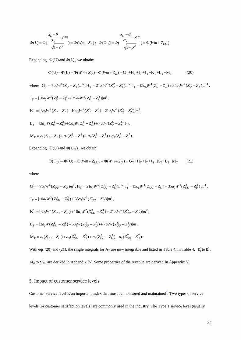
are defined in eq (19); E1, E3, M0 to M8 are derived in Appendix III.

20

1A1 E2

x c1

2

3A2 E2

x1 c

2

A3 (G I K M )x c8 6 4 2M M M M

2

A4 (F H J L )c x8 6 4 2

cM M M M

2

A5 (G I K M )6 4 2 0

cM M M M

2

C1 (G I K M )6 4 2 0

PcM M M M

2

C2 (F H J L )c8 6 4 2

PM M M M

2

' 'T 1 2A1 (E E )

2x c

LU

1

2 F

' 'T 3 4A2 (E E )

2x

LU

1 c

2 F

' ' ' ' ' ' 'T T T T T T T TA3 (G H I J +K L M )x c

8 7 6 5 4 3 2LU

M M M M M M M2 F

' ' ' ' ' ' 'T T T T T T T TA4 (G H I J +K L M )c x

7 6 5 4 3 2 1LU

cM M M M M M M

2 F

' ' ' ' ' ' 'T T T T T T T TA5 (G H I J +K L M )6 5 4 3 2 1 0

LU

cM M M M M M M

2 F

' ' ' ' ' ' ' ' ' ' ' ' ' 'T T T T T T T TC1 (G H I J +K L M )6 5 4 3 2 1 0

LU

PcM M M M M M M

2 F

' ' ' ' ' ' ' ' ' ' ' ' ' 'T T T T T T T TC2 (G H I J +K L M )c

7 6 5 4 3 2 1LU

PM M M M M M M

2 F

Table 4. The single integrals for eqs (9) and (16)

4.2.2 Revenue for correlated and truncated price and demand

We first define:

21

LL

x

xZ

,

21

UUU

x

xZ

then

21

2( ) ( ) ( )

1

L

xL

xm

L Wm Z

; U2

(U ) ( ) ( )1

U

xUU

xm

Wm Z

Expanding (U) and (L) , we obtain:

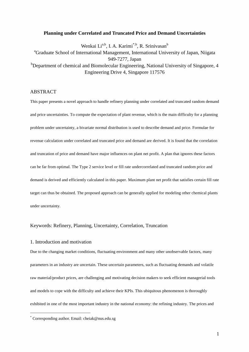
T T T T T T T(U) (L) ( ) ( ) G +H +I +J +K +L +MU LWm Z Wm Z (20)

where 6 6T 7G 7 ( )U La W Z Z m , 5 2 2 5

T 7H 21 ( )U La W Z Z m , 4 4 3 3 4T 5 7I [5 ( ) 35 ( )]U L U La W Z Z a W Z Z m ,

3 2 2 3 4 4 3T 5 7J [10 ( ) 35 ( )]U L U La W Z Z a W Z Z m ,

2 2 3 3 2 5 5 2T 3 5 7K [3 ( ) 10 ( ) 21 ( )]U L U L U La W Z Z a W Z Z a W Z Z m ,

2 2 4 4 6 6T 3 5 7L [3 ( ) 5 ( ) 7 ( )]U L U L U La W Z Z a W Z Z a W Z Z m ,

3 3 5 5 7 7T 1 3 5 7M ( ) ( ) ( ) ( )U L U L U L U La Z Z a Z Z a Z Z a Z Z .

Expanding (U) and U(U ) , we obtain:

' ' ' ' ' ' 'U T T T T T T T(U ) (U) ( ) ( ) G +H +I +J +K +L +MUU UWm Z Wm Z (21)

where

' 6 6T 7G 7 ( )UU Ua W Z Z m , ' 5 2 2 5

T 7H 21 ( )UU Ua W Z Z m , ' 4 4 3 3 4T 5 7I [5 ( ) 35 ( )]UU U UU Ua W Z Z a W Z Z m ,

' 3 2 2 3 4 4 3T 5 7J [10 ( ) 35 ( )]UU U UU Ua W Z Z a W Z Z m ,

' 2 2 3 3 2 5 5 2T 3 5 7K [3 ( ) 10 ( ) 21 ( )]UU U UU U UU Ua W Z Z a W Z Z a W Z Z m ,

' 2 2 4 4 6 6T 3 5 7L [3 ( ) 5 ( ) 7 ( )]UU U UU U UU Ua W Z Z a W Z Z a W Z Z m ,

' 3 3 5 5 7 7T 1 3 5 7M ( ) ( ) ( ) ( )UU U UU U UU U UU Ua Z Z a Z Z a Z Z a Z Z .

With eqs (20) and (21), the single integrals for AT are now integrable and listed in Table 4. In Table 4, '1E to '

4E ,

'0M to '

8M are derived in Appendix IV. Some properties of the revenue are derived In Appendix V.

5. Impact of customer service levels

Customer service level is an important index that must be monitored and maintained5. Two types of service

levels (or customer satisfaction levels) are commonly used in the industry. The Type 1 service level (usually

22

also called the confidence level) is the probability of not stocking out in all scenarios or horizons35

. The Type 2

service level (also often called the fill rate) is the proportion of demands that are met from a plant35

. The Type 1

service level is widely applied in chance constrained programming up to now. However, it is not how service is

interpreted in most applications35

. The Type 2 service level is a greater concern of most managers in industry6,35

.

The difference of Type 1 and 2 service level can be found in the literature6,35

.

5.1 Type 1 service level

To apply Type 1 service level on uncertain customer demand x, the following constraint should be added in the

model2,6

:

Pr D x

where α is the Type 1 service level or confidence level target, D is the production rate (no inventory) or the

deliverable amount (with inventory). The above constraint is transformed to the following by applying chance

constrained programming2,6

:

1( )D F (22)

In the above constraint, 1F is the reverse cumulative distribution function of the product demand. When

demand conforms to non-truncated normal distribution, constraint (22) becomes:

1( )xD (22a)

When demand conforms to doubly truncated normal distribution, constraint (22) becomes:

Pr ( )

L

D

BTN

x

D x x dx (22b)

where ( )BTN x is the bi-truncated density function of demand x:

23

( ) ( )

( ) .

[ ( ) ( )]

x xBTN

U L BTNx

x x

x x

xx x

where [ ( ) ( )]BTN x XU XLZ Z and UXU

x

xZ

, L

XL

x

xZ

.

let x

xt

and define XP

x

DZ

, then

( )

L

D

BTN

x

x dx =

2

21

2

XP

XL

Z t

x

BTN Z

e dt

= [ ( ) ( )]x

XP XL

BTN

Z Z

=

( ) ( )

( ) ( )

XP XL

XU XL

Z Z

Z Z

Thus, (22b) becomes

( ) ( )

( ) ( )

XP XL

XU XL

Z Z

Z Z

, or ( ) ( ) ( ( ) ( ))XP XL XU XLZ Z Z Z , i.e.,

1( ( ) ( ( ) ( )))x XL XU XLD Z Z Z (22c)

5.2 Type 2 service level

Type 2 service level is the one that most managers need6,35

. However, it cannot be accurately approximated by a

Type 1 service level6. To apply Type 2 service level on customer demand, the following constraint should be

added in the model6:

S

(23)

where β is the Type 2 service level or fill rate target defined by the decision maker, S is the actual amount of

product sold to customers. S/θrepresents the actual Type 2 service level. For non-truncated normally

distributed demand, the standard loss function, LF(.), has been effectively applied and approximated to compute

S in the literature6. In this paper, we extend the research to cases when demand is truncated.

5.3. The actual Type 2 service level

When demand x is doubly truncated, the actual amount of product sold to customers, SBTN, is the minimum value

of the customer demand and the production rate:

24

min{ , } ( )

U

L

x

BTN BTN

x

S P x x dx (24)

Expand eq (24), we have

( ) ( ) ( ) ( )

U U

L

x x

BTN BTN BTN BTN BTN

x P

S x x dx x P x dx LF P (25)

where BTN and ( )BTNLF P are the mean and the loss function of the bi-truncated normal demand,

respectively. Loss function represents the amount of unmet demand (the backorder level) of a plant facing

uncertain demand36

. BTN and ( )BTNLF P are derived in Appendix VI. From eqs (23) and (25), the actual

Type 2 service level for bi-truncated normal demand is:

( ) ( )1BTN BTN BTN BTN

BTN BTN BTN

S LF P LF P

(26)

Eq (23) then becomes:

( )1BTN BTN

BTN BTN

S LF P

(27)

6. The optimization model

The optimization model implementing the revenue calculation and the Type 1 and 2 service levels is shown as

follows:

p

p

P

max Revenue COSTS (eqs 9 or 16)

s.t. Constraints for Revenue (Tables 5 and 6)

Constraints for Type 1 or 2 service levels (eqs 22 and 27)

Constraints for COSTS

Other operational

constraints

where pRevenue is revenue from product p. The model is to maximize the net profit of a plant. We use the

formulae (eqs (9) or (16)) derived in this paper to calculate the actual revenue for each product. Tables 5 and 6

are used to support eqs (9) or (16). The constraints for Type 1 or 2 service levels are eqs (22) and (27),

respectively. COSTS includes the raw material cost, operating cost, inventory cost and investment cost, etc.

25

Other operational constraints, such as material balance and product quality, should also be included. Parameters

such as W, LZ , UUZ , XUZ , XLZ , M0 to M8, '0M to '

8M , LUF , BTN etc. should be calculated before running

the optimization model according to their definitions and the formulae derived in Appendixes III~VI.

7. Case Study

Two examples are used to illustrate the influences of correlation and truncation of price and demand on plant

revenue. Example 1 is taken from the case 1 of Li et al.6. Figure 3

6 shows the configuration of example 1.

MTBE and GASO (gasoline) enter the gasoline blending (GB) unit to produce two products: 90# (GASO’90)

and 93# (GASO’93) gasoline. The price of GASO and MTBE are 1400 and 3500 Yuan/tom, respectively. The

price of 90# and 93# gasoline are 3215 and 3387 Yuan/ton, respectively. The means of the demand for 90# and

93# gasoline are 50 and 70 tons, respectively. The octane number of GASO and MTBE are 70 and 101,

respectively. The octane number of 90# and 93# gasoline are 90 and 93, respectively. The blending requirement

is that the octane number of each product should equal or be greater than the required octane number of that

product. No inventory is considered and the overproduced products are assumed to be valueless. All examples

are formulated with GAMS37

. The solver MINOS5 in GAMS 21.7 is used for NLP.

10.1 Accuracy of different approximation functions

GASO’90

GASO’93 GASO

MTBE

G90

G93

M90

M93

Figure 3 The configuration of example 1

Gasoline Blending Unit

26

In this case, the correlation coefficients between all products and their prices are set to zero and hence the

normally distributed price and demand becomes independent. The results from eq (9) should then be the same as

that obtained from the literature6. The standard deviation of 90# and 93# gasoline demands are both 10 tons.

In Table 5.1, the result of the first row is taken from the case 1 of Li et al.6 Rows 2 to 4 are results from (.)

approximation methods with three orders (5th

, 7th

, 9th

). It can be seen that, all three approximation methods have

rather high accuracy. The polynomial approximation with higher order has higher accuracy. For the sake of

simplicity, seventh order polynomial function is used to approximate the standard normal cumulative function in

this paper because it has high enough accuracy. Our formulae involve more equations and variables and thus,

the solution time is longer than that in the literature6. In this small case study, the solution times of all methods

are similar.

Net Profit Gap (%) Solution time

(s)

SINGLE

EQUATIONS

SINGLE

VARIABLES

Li et al. 2004 38733.69 0.03 11 13

5th

polynomial 38882.36 0.38 0.04 37 39

7th

polynomial 38685.95 -0.12 0.05 41 43

9th

polynomial 38717.32 -0.04 0.05 47 49

Table 5.1 Accuracies of different polynomial functions

In Table 5.2, the revenue calculated from eq (9) using GAMS for 90# gasoline is compared with the result by

integrating eq (3) directly using MATLAB,38

at different correlation coefficients. The price and demand are

non-truncated and the standard deviation of 90# gasoline is 300 Yuan/ton. The production rate of 90# gasoline is

fixed to 39.565 at all correlation coefficients. MATLAB

uses rigorous double integral to compute revenue and

thus accurate. We can see that the gap between the approximation formulae and MATLAB

is very small. It is

difficult to implement MATLAB

into refinery planning model because MATLAB

takes very long time to

compute eq (3) and it is difficult to iteratively communicate MATLAB

with an optimization solver.

27

MATLAB 7

th polynomial

approximation Gap,%

0.0 1.24740E+05 1.24720E+05 -0.016

0.1 1.24780E+05 1.24760E+05 -0.016

0.2 1.24830E+05 1.24810E+05 -0.016

0.3 1.24870E+05 1.24850E+05 -0.016

0.4 1.24920E+05 1.24900E+05 -0.016

0.5 1.24960E+05 1.24950E+05 -0.008

Table 5.2 Comparison with MATLAB

10.2. Effect of correlation

In this case, we consider the influence of correlation coefficient on plant revenue at different CVs (Coefficient

of Variation, the ratio of the standard deviation σ to the meanμ: CV= / ). The standard deviation of 90#

and 93# gasoline at different CVs are listed in Table 6. The standard deviation of 90# and 93# gasoline prices at

different CVs are assumed to be fixed at 600 and 620 Yuan/ton, respectively.

CV

Products 0.2 0.3 0.5

90# gasoline 10 15 25

93# gasoline 10 20 35

Table 6 Standard deviation of products at different CVs for example 1

Net Profit,

Yuan Difference,%

0 10097.50 0.0

0.1 10589.83 4.9

0.2 11096.87 9.9

0.3 11638.74 15.3

0.4 12225.64 21.1

0.5 12853.69 27.3

Table 7 Effect of correlation at CV=0.5 in example 1

The net profits at different correlation coefficients at CV=0.5 are listed in Table 7 (the correlation coefficients

between all products and their demands are set to be the same). It can be seen that, the net profit at correlation

28

coefficient of 0.4 (near the real world data) is 21.1% higher than the net profit calculated by assuming

independent demand and price (correlation coefficient=0.0). That means, if for a large enough CV of a product,

assuming independent price and demand may underestimate the net profit by up to 21%. Note that when the

correlation coefficient is too high (bigger than 0.6), the net profit will decrease significantly.

In general, the revenue difference between the independent and correlated cases depends on the CV of products.

In the problem studied here, if the CV of a product takes value of 0.2, the net profit difference between =0.4

and =0 is about 2%. This difference is about 5% for CV of 0.3. We set =0.4 for correlated demand and price

because it near the real world value according to the regressed data from EIA9. If is set to be a constant, then

as the standard deviation of price increases, the revenue increases slightly. However, as the standard deviation of

demand increases, the revenue decreases significantly.

10.3 Effect of Truncation

Integrating over the whole range of a normal distribution may give incorrect results to revenue calculation. The

formulae derived for bivariate double-truncated normal distribution are applied in the model. The results are

shown in Tables 10 and 11 (the product production rates of truncated cases are fixed to those of the

non-truncated case for fair comparison). In Table 8 (at CV=0.2), it can be seen that, if the price and demand

vary inside two standard deviations of their mean values, integrating over the whole range will underestimate

the revenue by 2 to 3%. If the price and demand vary inside one standard deviation of their mean values,

integrating over the whole range will underestimate the revenue by about 12%. The revenue difference between

truncated and non-truncated becomes much more significant for large enough CV. In Table 8 (at CV=0.5),

integrating over the whole range will underestimate the revenue from 20% up to 130%.

29

CV=0.2 CV=0.5

Integration

Range of

Non-truncated

case

Integration Ranges of

Truncated Cases

Integration

Range of

Non-truncated

case

Integration Ranges of

Truncated Cases

(–, +) (+/–2) (+/–) (–, +) (+/–2) (+/–)

0 38685.9 39847.6 43513.6 10097.5 14986.6 23935.1

0.1 38851.2 39948.7 43772.7 10589.8 15234.4 24545.5

0.2 39021.0 40107.0 43958.2 11096.9 15556.8 25030.0

0.3 39202.3 40418.5 44166.1 11638.7 16067.2 25457.7

0.4 39398.5 40792.3 44369.3 12225.6 16693.6 25907.6

0.5 39608.6 39418.8 44445.2 12853.7 15504.5 26286.5

Table 8 Effect of truncation at CV=0.2 and CV=0.5 in example 1

10.4 Effect of customer service levels

Table 9 lists the net profits when the constraints for Type 1 and 2 service levels are added into the model. The

price and demand vary inside two standard deviations of their mean values. The CVs of demand and price are

set to 0.2. The net profits in the second column (No C.L./F.L.) are slightly higher than those in the third column

of Table 8 because the product production rates are free to change in this case.

It can be seen that, the net profit decreases when we set Type 1 service level target to 0.5. This is because the

production rate has to be greater than certain value to satisfy the customer demand. Even though a 50% of

confidence level seems to be low, the actual fill rates achieved are high enough: 92.% and 94.8% for product 1

and 2, respectively. In this case, the gap between these two service levels is rather big. When fill rate is set to 0.9,

the net profit decreases by about 7~10% compare to “No C.L./F.L.” case. In this case, the net profit becomes

negative (-38408.2 Yuan at =0.4) when we set too high C.L. target (e.g., 95%). The plant loses money if the

customer demand has to be satisfied at too high ratio. A planning strategy taking Type 1 service level target into

account only might be thus suboptimal. A plant has to compromise between the net profit and the two service

30

levels. In fact, when C.L. is 95%, the actual fill rates for product 1 and 2 are both 99.9%, which are

unnecessarily high. In this case, setting a Type 2 service level target, F.L.=0.9, is a better choice.

No C.L./F.L. C.L.=0.5 F.L.=0.90

0 39885.4 28469.6 35868.0

0.1 39980.6 28877.1 36136.1

0.2 40135.6 29373.0 36478.4

0.3 40445.1 30052.0 36987.2

0.4 40817.8 30805.2 37557.8

0.5 39439.4 29713.7 36318.7

No C.L./F.L.: No service level constraints are added;

C.L.: Type 1 service level constraint is added;

F.L.: Type 2 service level constraint is added.

Table 9 Net profit at different service levels at CV=0.2 in example 1

10.5 Example 2

A larger size example (example 2) was used to illustrate the results using our derived formula. A process flow

diagram of a refinery plant is shown in Figure 4. Details of this example can be found in Li et al.39,40

. The

problem contains three main production units: CDU (Crude Distillation Unit), GB (Gasoline Blending) and DB

(Diesel Oil Blending). Crude oil is separated into three fractions by CDU. Gasoline and MTBE enter the GB to

produce two products: 90# gasoline and 93# gasoline. Diesel oil and naphtha enter the DB to produce another

two products: -10# diesel and 0# diesel. The prices (Yuan/ton) of the raw materials and the products are listed in

Table 10. The capacity of the CDU is 400 ton/day; the CDU operation cost is 20 Yuan/ton/day. The CDU

transfer ratios of crude oil to gasoline, to diesel oil, and to naphtha are fixed at 0.2, 0.3 and 0.5, respectively. The

market demands for 90# gasoline and 93# gasoline are assumed to conform to normal distributions, N(50, 25)

and N(40, 25), respectively. For the sake of simplicity, the market demands for the other two products are

assumed to be deterministic without losing the generality of the model. The objective of this case study is to

determine the optimal planning strategy for the refinery under uncertain market conditions. The results are

shown in Table 11.

31

C

D

U

GASOLINE

G

B

D

B

NAPHTHA

DIESEL OIL

90 # GASOLINE

93 # GASOLINE

-5 # DIES OIL

0 # DIESEL OIL

MTBE

CRUDE OIL

In Table 11, it can be seen that, as increases, the net profit increases along each column. In the second and

third column, confidence level and fill rate are considered and assumed to be 95%. The net profit reduced by

around 30% and 12% when C.L. and F.L. are set to 95%, respectively. In the truncated case, the net profit

increases by 1.4% to 4.5% when the degree of truncation is (+/–2). The net profit increases by 14.8% to

22.3% when the degree of truncation is (+/–).

Table 10 Price Data (Yuan/ton) for example 2

Figure 4 The configuration of example 2

Non-truncated Truncated

No. C.L./F.L. C.L.=0.95 F.L.=0.95 (+/–2) (+/–)

0 120,118.8 81,967.0 102,912.8 125,549.6 146,859.5

0.1 121,971.4 84,814.5 105,452.8 126,730.4 147,108.9

0.2 123,843.1 87,698.7 107,975.3 128,044.3 147,388.0

0.3 125,730.8 90,600.8 110,494.3 129,586.9 147,776.8

0.4 127,632.7 93,495.6 113,026.5 131,271.3 148,242.2

0.5 129,551.4 96,490.6 115,577.7 131,312.3 148,690.1

Table 11 Results from example 2

Raw Material Products

Crude Oil MTBE 90# gasoline 93# gasoline -5# diesel 0# diesel

1400 3500 3215 3387 2700 2500

32

12. Conclusion

In this paper, the correlation between price and demand as well as their integration ranges are studied.

Theoretical derivations are performed and several case studies are developed to study the influences of

correlation and truncation on plant revenue. Case studies show that, for a large enough CV of a product,

assuming independent price and demand may underestimate the revenue by up to 20%. Since the real world

demands or prices vary in limited ranges, integrating over the whole range of a normal distribution, which some

research has done, may give incorrect results. This paper thus approximates a bivariate double-truncated normal

distribution for demand and price. Case studies show that the degree of truncation can significantly influence the

on plant revenue.

To handle possible unmet customer demands, the hard-to-specify penalty functions of the two-stage

programming are avoided and replaced by two of the decision maker’s service level targets, namely the

confidence level and fill rate target. Confidence level or the Type 1 service level is commonly used in

chance-constrained programming. However, fill rate or the Type 2 service level is a greater concern of most

managers. Two types of service levels, Type 1 and 2, are implemented into the planning model in this paper.

Case studies show that a planning strategy that satisfies certain confidence level targets might be too generous

compared to a strategy that satisfies a fill rate target. Case studies including refinery planning problems were

used to illustrate the proposed approach.

33

Literature Cited

(1) Gupta, A.; Maranas, C. D. Managing demand uncertainty in supply chain planning, Comput. Chem. Eng., 2003, 27,

1219.

(2) Li, P.; Moritz Wendt; Günter Wozny Optimal Operations Planning under Uncertainty by Using Probabilistic

Programming, Proceedings Foundations of Computer-Aided Process Operations (FOCAPO 2003), Coral Springs,

Florida, USA, January 12-15, 2003.

(3) Rooney, W. C.; Biegler, L. T. Optimal process design with model parameter uncertainty and process variability, AIChE

J, 2003, 49, 438.

(4) Petkov, S. B.; Maranas, C. D. Multiperiod planning and scheduling of multiproduct batch plants under demand

uncertainty, Ind. Eng. Chem. Res., 1997, 36 4864-4881.

(5) Jung, J. Y.; Blau, G.; Pekny, J. F.; Reklaitis G. V.; Eversdyk, D. A simulation based optimization approach to supply

chain management under demand uncertainty, Comput. Chem. Eng. 2004, 28 (10), 2087–2106.

(6) Li W. K.; Chi-Wai Hui; Pu Li; An-Xue Li Refinery planning under uncertainty, Ind. Eng. Chem. Res. 2004, 43,

6742-6755.

(7) Roberto A. De Santis, Crude oil price fluctuations and Saudi Arabia's behaviour, Energy Economics, 2003, 25(2),

155-173.

(8) Cooper, John C.B. Price elasticity of demand for crude oil: estimates for 23 countries. OPEC Review, 2003, 27 (1), 1-8.

(9) The U.S. Energy Information Administration, http://www.eia.doe.gov

(10) Jensen, J.L., Lake, L.W., Corbett, P.W.M., and Goggin, D.J., Statistics for petroleum engineers and geoscientists, New

Jersey, Prentice Hall, 1997.

(11) Thomopoulos, N.T., Applied Forecasting Methods, Prentice-Hall, Englewood Cliffs, New Jersey, 1980.

34

(12) Bookbinder, J.H., and A.E. Lordahl, Estimation of Inventory Re-Order Levels Using the Bootstrap Statistical Procedure,

IIE Transactions, 1989, 21, 302-312.

(13) Johnson, A.C., and Thomopoulos, N.T., Use of the Left-Truncated Normal Distribution for Improving Achieved

Service Levels, Proceedings of the Decision Sciences Institute, 2002, 2033-2041.

(14) Johnson, A.C., and Dhungel, B.K., Approximation of the Cumulative Distribution Function of the Bivariate Truncated

Normal Distribution, Proceedings of the Decision Sciences Institute, 2003, 3111-3118.

(15) Clay, R.L.; Grossman, I.E. A disaggregation algorithm for the optimization of stochastic planning models, Comput.

Chem. Eng., 1997, 21, 751.

(16) Kall, P.; Wallace, S. W. Stochastic programming. New York: Wiley, 1994.

(17) Zimmermann H.J. An Application-Oriented View of Modeling Uncertainty. Eur. J. Oper. Res. 2000, 122, 190-198.

(18) Kim, K. J.; Diwekar, U. M. Efficient Combinatorial Optimization under Uncertainty. 1. Algorithm Development, Ind.

Eng. Chem. Res., 2002, 41 1276.

(19) Applequist, G. E.; Pekny, J. F.; Reklaitis, G. V. Risk and uncertainty in managing chemical manufacturing supply

chains, Comput. Chem. Eng. 2000, 24, 2211-2222.

(20) Ierapetritou, M.G.; Pistikopoulos, E.N. Batch Plant Design and Operations under Uncertainty, Ind. Eng. Chem. Res.,

1996, 35 772.

(21) Liu, M. L.; Sahinidis, N.V. Optimiztion in Process Planning under Uncertainty Ind. Eng. Chem. Res., 1996, 35 4154.

(22) Dantzig, G. B. Linear programming under uncertainty, Management Science, 1955, 1:197-206.

(23) Wellons, H.S.; Reklaitis, G. V. The design of Multiproduct batch plants under uncertainty with stage expansion,

Comput. Chem. Eng., 1989, 13, 115-126.

(24) Yi G.; Reklaitis G.V. Optimal design of batch-storage network with uncertainty and waste treatments, AIChE J., 2006,

52 (10), 3473-3490.

35

(25) Lee, Y. G.; Malone, M. F. A General Treatment of Uncertainties in Batch Process Planning, Ind. Eng. Chem. Res.,

2001, 40 1507

(26) Neiro, S.M.S.; Pinto, J., Supply Chain Optimization of Petroleum Refinery Complexes, The Foundations of Computer

Aided Process Operations Conference (FOCAPO 2003), Coral Springs, Florida, USA, January 12-15, 2003.

(27) Balasubramanian J.; Grossmann I.E. Approximation to multistage stochastic optimization in multiperiod batch plant

scheduling under demand uncertainty, Ind. Eng. Chem. Res. 2004, 43 (14): 3695-3713.

(28) Janak S.L.; Lin X.X.; Floudas C.A. A new robust optimization approach for scheduling under uncertainty - II.

Uncertainty with known probability distribution, Comput. Chem. Eng., 2007, 31 (3), 171-195.

(29) Bonfill A.; Espuna A.; Puigjaner L. Addressing robustness in scheduling batch processes with uncertain operation times

Ind. Eng. Chem. Res. 2005, 44 (5), 1524-1534.

(30) Applequist, G. E.; Pekny, J. F.; Reklaitis, G. V. Risk and uncertainty in managing chemical manufacturing supply

chains, Comput. Chem. Eng. 2000, 24, 2211-2222.

(31) Chen C.L.; Lee W.C. Multi-objective optimization of multi-echelon supply chain networks with uncertain product

demands and prices, Comput. Chem. Eng., 2004, 28 (6-7): 1131-1144.

(32) Guillen G.; Mele FD.; Espuna A. et al. Addressing the design of chemical supply chains under demand uncertainty, Ind.

Eng. Chem. Res. 2006, 45 (22), 7566-7581.

(33) Mele F.D.; Guillen G.; Espuna A. et al. An agent-based approach for supply chain retrofitting under uncertainty,

Comput. Chem. Eng., 2007, 31(5-6), 722-735.

(34) Abramowitz & Stegun, Handbook of Mathematical Functions, Dover Publications, 1965.

(35) Nahmias, S. Production and operations analysis, McGraw-Hill, 2001.

(36) Hopp, W. J.; Spearman, M. L. Factory Physics: foundations of manufacturing management, Irwin/McGraw-Hill, 2000.

36

(37) Brooke, A.; Kendrik, D.; Meeraus, A.; Raman, R.; Rosenthal, R. E. GAMS—A User’s Guide; GAMS Development

Corporation, Washington DC, 1998.

(38) Works, T. M. MATLAB 7.0 (R14) User’s Manual; The MathWorks Inc., Natick, MA, 2004.

(39) Wenkai L.; Hui CW; Anxue L. New Methodology enhances planning for refined products, Hydrocarbon Processing,

2003, 82(10), 81-88.

(40) Li, W.; Hui, C. W. Applying Marginal Value Analysis in Refinery Planning, Chem. Eng. Comm., 2007, 194(7),

962-974.

37

Appendix I Real world correlation coefficient estimation between demand and price

We estimate the correlation coefficients between demand and price for world crude oil and gasoline by

regressing the real world 2003-2004 data from EIA9.

The mean and standard deviation of the price and demand are estimated using:

1

n

i

i

x

xn

(A1.1)

2

1

( )

1

n

i

i

x x

n

(A1.2)

where, xi is the sample data from EIA and n is the total number of sample data. x and are the UMVUE

(Uniformly Minimum Variance Unbiased Estimators) of the mean and standard deviation.

The sample correlation coefficient is used as the estimator for 10

:

1

2 2

1 1

( )( )

( ) ( )

n

i i

i

n n

i i

i i

c c x x

c c x x

(A1.3)

where, xi and ci are the sample demand and price data respectively. x and c are obtained using (A1.1).

The correlation coefficient between gasoline (New York Harbor Gasoline Regular) price and demand is 0.44

and 0.30 for world crude oil for year 2003 and 2004 using eq (A1.3) and the real world data from EIA. Figure

A.1 shows the profile of the world crude oil demand and price (EIA). In Figure A.1, the crude oil price increases

generally as the increase of crude oil demand.

38

Figure A.1 World* crude oil demand vs. crude oil price

**(2003-2004)

*: Refers to total OECD which includes OECD Europe, Canada, Japan, South Korea, United States, and Other.

**: Brent (US. Dollars per Barrel)

Appendix II The range of x

To increase accuracy, the polynomial approximation function, eq (17), is regressed in the range [–3, 3] and [–5,

5] because the domain of (x) used in the single integrals locates in this range with high probability.

For a normal distribution with mean and standard deviation , we have

{ } 0.9545

{ } 0.9973

Pr 2 x 2

Pr 3 x 3

where Pr is the operator of the probability computation. In other words, there is a possibility of 99.73% that x

locates in the range [–3, +3]. We have

U2 2

U1 1

U U

x x c

x x c cm

and 2 2

L1 1

L L

x x c

x x c cm

.

In the above equations, with a 99.73% confidence, when U xx 3 and cc c 3 , UU is at its the upper

bound, UB

UU ; when L xx 3 and cc c 3 , L is at its the lower bound, LBL .

Thus, with a 99.73% confidence, we have the range of UU and L:

World Crude Oil Demand vs. crude oil Price(2003-2004)

20

25

30

35

40

45

50

1 2 3 4 5 6 7 8 9 10 11 12 13 14 15 16 17 18 19 20 21 22 23 24

Month

US

$/B

arr

el

46

47

48

49

50

51

52

53

Mil

lion b

arr

els

/day

price

demand

39

x c

UB x cU

2 2

3 c 3 c

3 3U

1 1

x c

LB x c

2 2

3 c 3 c

3 3L

1 1

As P locates in the range [XL, XU], the range of U locates between UU and L.

Similarly, we can obtain the ranges when the confidence is 95.45%. Table A.1 lists the ranges of L, U and UU at

different confidences and correlation coefficients. When the degree of truncation is 2 , the ranges of L, U

and UU are listed in the first row of Table A.1 at different correlation coefficients. In this situation, we use [–3, 3]

as the range of x and set a0~an in eq (17) to values in the row [–3, 3] in Table 3. When the the degree of

truncation is , the ranges of L, U and UU are narrower than those in first row of Table A.1. Thus, we also

can use [–3, 3] as the range of x. When the degree of truncation is 3 , we use [–5, 5] as the range of x and

set a0~an in eq (17) to values in the row [–5, 5] in Table 3.

0 0.1 0.4 0.5

Range (95.45% confidence) [–2.0, 2.0] [–2.2, 2.2] [–3.1, 3.1] [–3.5, 3.5]

Range (99.73% confidence) [–3.0, 3.0] [–3.3, 3.3] [–4.6, 4.6] [–5.2, 5.2]

Table A.1 Range of x

Appendix III Some frequently used integrals for eq (9)

We derive the frequently used integrals in eq (9) (listed in Table 4) in this section.

40

22 2 2

2 22 2 2

2 2

2 22

2

2

( )U

2 2 2 21

[(1 )( ) ]1 1

2

(1 )( )1 1( )2 1 2

E

U

U UU

U

U

Wm Zm m

m m

WZ W ZW m Z

W W

m

WZW m

Z W

W

m

me e dm me e dm

me dm

e me dm

Let 2

21 ( )

1

UWZt W m

W

, then

2 2

2

2 2 2

2

2

2

1( )

2 1 21 22 2

1( )

2 1 2 22 3

2 2

1( )

2 13

2 2

1E ( )

11 1

1 [

1(1 )

2

(1 )

U

U

U

Z t

UW

Z t t

UW

Z

UW

WZte e dt

WW W

WZe te dt e dt

WW

WZe

W

(A3.1)

Similarly,

22 2

22 2 2 2

2

1(1 )( ) ( )1U 1 2 1( )2 12 2 2

32

E 21

U U

U

WZ ZW mZm W WW

m m

ee e dm e e dm

W

(A3.2)

2

20 2

m

m

M e dm

,

2

21 0

m

m

M me dm

2 2 2 2

2 2 2 2 22 0( ) |

m m m m

m m m

M m e dm md e me e dm M

2

3 23 0

m

m

M m e dm

,

2

4 24 3 2

m

m

M m e dm

In general,

2

2 22

1

2 (2 2 1)

m nn

n

im

M m e dm n i

, n=1,2,3,… (A3.3)

2

2 1 22 1 0

m

nn

m

M m e dm

, n=1,2,3,… (A3.4)

41

Appendix IV Some frequently used integrals for eq (16)

We derive the frequently used integrals in eq (16) (listed in Table 4) in this section.

Define L

c

c ca

, U

c

c cb

, we have

2 222 2 2

2

(1 )( )1U 1( )

' 2 12 2 21E

UU

c U

L

c

c c WZW m

Z bm W

W

ac cm

me e dm e me dm

let 2

21 ( )

1

UWZt W m

W

, then

2 21

2

1

2 2 21 1

2

1( )

' 2 1 21 22 2

1 ( ) ( )( )

2 1 2 21 12 3

2 2

1E ( )

11 1

1 ( ) 2 [ ( ) ( )]

1(1 )

EU

E

U E E

UZ t

UW

L

Z U L

UWE E

WZte e dt

WW W

WZe e e U L

WW

(A4.1)

where 21

21

1

UE

WZL a W

W

, 2

12

11

UE

WZU b W

W

. Similarly,

2 2

2 2 22 2

2

L

' 2 22

1 ( ) ( )( )

2 1 2 22 22 3

2 2

E

1 ( ) 2 [ ( ) ( )]

1(1 )

L E E

b m

a

Z U L

LWE E

me e dm

WZe e e U L

WW

(A4.2)

where 22

21

1

LE

WZL a W

W

, 2

22

11

LE

WZU b W

W

.

2

2 22

1( )U 2 1

' 2 23 1 1

2E 2 [ ( ) ( )]

1

UZb m

W

E E

a

ee e dm U L

W

(A4.3)

2

2 22

1( )L 2 1

' 2 24 2 2

2E 2 [ ( ) ( )]

1

LZb m

W

E E

a

ee e dm U L

W

(A4.4)

2

' 20 2 [ ( ) ( )]

b m

a

M e dm b a

,

2 2 2

' 2 2 21 ( )

b m b a

a

M me dm e e

In general,

42

2 2 2 2

2 2

2

' 1 1 22 2 2 2

1 1 '2 2

( ) | ( 1)

= [ ] ( 1) , 2,3,4,...n

b b bm m m m

n n n b nn a

a a a

b a

n n

M m e dm m d e m e n e m dm

b e a e n M n

(A4.5)

Appendix V Properties of the revenue

In this appendix, we show that revenue formulae for correlated and truncated, eq (9) and eq (16), can be reduced

to the formulae appeared in the literature when demand and price are independent and non-truncated. The

normally distributed price and demand are independent if =0. In this situation, we have

20

1W

,

2U

1U

xx

P PZ

, U becomes a constant.

From Table 2,

U U U

A1 0

2 2 2 2 2m m2x c x c x c2 2 2 2 2

1

m m

1me e dm e me dm e M

2 2 2

U U U

A2

2 2 2 2 2m m2x x x2 2 2 2 2

m m

1 c c ce e dm e e dm e

2 2 2

A3 =0,

A4 (U) (U) 0

2 2m m

c x c2 2

m m

cme dm me dm

2 2

A5 (U) (U) (U)

2 2m m

2 2

m m

c ce dm e dm c

2 2

From eq (6),

2 2

2 2

C1= (U) (U) (U)2 2

m m

m m

e ePc dm Pc dm Pc

43

2 2

2 2

C2= (U) (U) 02 2

m m

c c

m m

e eP m dm P m dm

.

Thus, from eq (9),

Revenue = A1 + A2 + A3 + A4 + A5 + B – C1 – C2=

U

( ) (U)

2

x 2c

e c P Pc2

= ( ) ( ) ( )xx x

P Pc c P Pc

= ( ) [1 ( )]x

x x x

P P Pc c

where (.) is the standard normal density function,

2

21

( )2

t

x e

. The above equation has reduced to the

formulae appeared in the literature4,6

. This also proves that, underlying the formulae used in the literature, the

demand and price are assumed to be independent and take values in the range (–, +).

It is also easy to show that, when Ux and Lx , Uc and Lc , the equation for

truncated and correlated revenue, eq (16), is reduced to the equation for non-truncated and correlated revenue,

eq (9). In fact, when Lx then

2L

2 0e

, (L) 0 ; when Ux then UU , U(U ) 1 .

We also have 1LUF . Thus, the single integrals for AT tend to the single integrals for A (Table 2), i.e.,

T TA1 ~A5 A1~A5 , respectively. Furthermore, TC1 C1=B C1Pc ; TC2 C2 . Hence, eq (16) reduces

to eq (9).

Appendix VI Derivation of the bi-truncated expectation and loss function

The expectation of the bi-truncated normal demand, BTN , is:

1( ) ( )

U U

L L

x x

BTN BTNBTN xx x

xx x dx x dx

44

let x

xt

, then

2 2 22

2 2 2

2

1( )

2 2 2

[ ( ) ( )] [ ( ) ( )]

XU XU XU

XL XL XL

Z Z Zt t t

x x xBTN x

BTN BTN BTNZ Z Z

x xXU XL XU XL

BTN BTN

t e dt te dt e dt

Z Z Z Z

Since [ ( ) ( )]BTN x XU XLZ Z , we have

( ) ( )

( ) ( )

XU XLBTN x

XU XL

Z Z

Z Z

(A5.1)

The bi-truncated loss function, ( )BTNLF P , is:

1( ) ( ) ( ) ( ) ( )

U U UX X X

BTN BTN

BTN x BTN xP P P

x P xLF P x P x dx x dx dx

let x

xt

and define XP

x

PZ

, then

2 2

2 2 2

2 2

2

2 2 2

1( ) ( )

2 2

2 2 2

XU XU

XP XP

XU XU XU

XP XP XP

Z Zt t

x xBTN x

BTN BTNZ Z

Z Z Zt t t

x xX

Z Z ZBTN BTN BTN

PLF P t e dt e dt

Pte dt e dt e dt

Thus

( )( ) { [ ( ) ( )] [ ( ) ( )]}x

BTN x XU XP XU XP

BTN BTN

PLF P Z Z Z Z

(A5.2)

When the demand conforms to left truncated normal distribution, that is, UX and XUZ , we have

( ) 1, ( ) 0XU XUZ Z and [1 ( )]BTN LTN x XLZ . Thus the left truncated loss function, ( )LTNLF P ,

is

( ) ( )( ) { [1 ( )]}x XP

LTN x XP

LTN LTN

Z PLF P Z

(A5.3)

When the demand conforms to right truncated normal distribution, i.e., LX and XLZ , then

( ) 0, ( ) 0XL XLZ Z and ( )BTN RTN x XUZ . Thus the right truncated loss function, ( )RTNLF P , is

( )( ) [ ( ) ( )] [ ( ) ( )]

( ) ( )

xRTN XU XP XU XP

XU XU

PLF P Z Z Z Z

Z Z

(A5.4)

For non-truncated normal distribution, i.e., UX and LX , we have XUZ and XLZ

and BTN x . Eq (A5.2) is reduced to

45

( ) { ( ) [1 ( )]}x XP XP XPLF P Z Z Z (A5.5)

The above formula can also be found in the literature4,6

.