plantsafety(cdi)
DESCRIPTION
Industrial Facility SafetyTRANSCRIPT

JJ OO ÃÃ OO LL UU ÍÍ SS SS AA NN TT OO SS
IINNDDUUSSTTRRIIAALL FFAACCIILLIITTYY SSAAFFEETTYY CCOONNCCEEPPTTIIOONN,, DDEESSIIGGNN AANNDD IIMMPPLLEEMMEENNTTAATTIIOONN
22000099

II NN DD UU SS TT RR II AA LL FF AA CC II LL II TT YY SS AA FF EE TT YY
AA BB OO UU TT TT HH EE AA UU TT HH OO RR The author is a professional engineer and an independent consultant with more than ten years of industrial experience in chemical, petroleum and petrochemical industries where he designed process safety systems and made industrial risk analysis, performed safety reviews, implemented compliance solutions, and participated in process safety management (PSM). The author holds a Bachelor (B. Eng.) degree in Chemical Engineering and Licentiate (Lic. Eng.) degree in Chemical Engineering from School of Engineering of Polytechnic Institute of Oporto (Portugal), and a Master (M. Sc.) degree in Environmental Engineering from Faculty of Engineering of the University of Oporto (Portugal). Also, he has an Advanced Diploma in Safety and Occupational Health from the Institute for Welding and Quality (ISQ) and he is licensed and certified by ACT (National Examination Board in Occupational Safety and Health, Work Conditions National Authority). Notice This report was prepared as an account of work sponsored by Risiko Technik Gruppe (RTG). Reference herein to any specific commercial product, process, or service by trade name, trademark, manufacturer, or otherwise, does not necessarily constitute or imply its endorsement, recommendation, or favoring by the Risiko Technik Gruppe, any agency thereof, or any of their contractors or subcontractors. Available to the public from the sponsor agency: Risiko Technik Gruppe Office of Scientific and Technical Information can be requested to: E-Mail: [email protected] Website: http://www.geocities.com/risiko.technik/index.html Available to the public from the author: E-Mail: [email protected]

CC OO NN CC EE PP TT II OO NN ,, DD EE SS II GG NN ,, AA NN DD II MM PP LL EE MM EE NN TT AA TT II OO NN
TTEERR MMIINNOOLLOOGGYY AIChE American Institute of Chemical Engineers. BPCS Basic Process Control System. CCPS Center for Chemical Process Safety. CDF cumulative distribution function. DCS Distributed Control System. Electrical / Electronical / Programmable Electronical Systems (E/E/PES) A term used to embrace all possible electrical equipment that may be used to carry out a safety function. Thus simple electrical devices and programmable logic controllers (PLCs) of all forms are included. Equipment Under Control (EUC) Equipment, machinery, apparatus or plant used for manufacturing, process, transportation, medical or other activities. ESD Emergency shut-down. ETA Event Tree Analysis. FME(C)A Failure Mode Effect (and Criticality) Analysis. FMEDA Failure Mode Effect and Diagnostics Analysis. FTA Fault Tree Analysis. Hazardous Event hazardous situation which results in harm. HAZOP Hazard and Operability study. HFT Hardware failure tolerance. IEC EN 61508 Functional safety of electrical / electronical / programmable electronical safety-related systems. IEC EN 61511 Functional safety, safety instrumented systems for the process industry sector.

II NN DD UU SS TT RR II AA LL FF AA CC II LL II TT YY SS AA FF EE TT YY
IPL Independent Protection Layer. ISA The Instrumentation, Systems, and Automation Society. LOPA Layer of Protection Analysis. Low Demand Mode (LDM) Where the frequency of demands for operation made on a safety related system is no greater than one per year and no greater than twice the proof test frequency. MTBF Mean time between failures. PDF Probability density function. PFD Probability of failure on demand. PFH Probability of dangerous failure per hour. PHA Process Hazard Analysis. PLC Programmable Logic Controller. SFF Safe failure fraction. SIF Safety instrumented function. SIL Safety integrity level. SIS Safety instrumented system. SLC Safety life cycle. Safety The freedom from unacceptable risk of physical injury or of damage to the health of persons, either directly or indirectly, as a result of damage to property or the environment Safety Function Function to be implemented by an E/E/PE safety-related system, other technology safety-related system or external risk reduction facilities, which is intended to achieve or maintain a safe state for the EUC, in respect of a specific hazardous event.

CC OO NN CC EE PP TT II OO NN ,, DD EE SS II GG NN ,, AA NN DD II MM PP LL EE MM EE NN TT AA TT II OO NN
Tolerable Risk Risk, which is accepted in a given context based upon the current values of society.

II NN DD UU SS TT RR II AA LL FF AA CC II LL II TT YY SS AA FF EE TT YY
CCOONNTT EENNTT Preface 8 Safer Design and Chemical Plant Safety 9
Introduction to Risk Management 9 Risk Management 10 Hazard Mitigation 11
Inherently Safer Design and Chemical Plant Safety 12 Inherently Safer Design and the Chemical Industry 13
Control Systems Engineering Design Criteria 16 Codes and Standards 16 Control Systems Design Criteria Example 16
Risk Acceptance Criteria and Risk Judgment Tools 18 Chronology of Risk Judgment Implementation 19 Conclusions 23
References 24 Safety Lvel Integrity (SIL) 25
Background 25 What are Safety Integrity Levels (SIL) 25 Safey Life Cycle 26
Risks and their reduction 28 Safety Integrity Level Fundamentals 28
Probability of Failure 29 The System Structure 30 How to read a safety integrity level (SIL) product report? 32 Safety Integrity Level Formulae 33
Methods of Determining Safety Integrity Level Requirements 34 Definitions of Safety Integrity Levels 34 Risk Graphic Methods 36 Layer of Protection Analysis (LOPA) 42 After-the-Event Protection 44 Conclusions 45
Safety Integrity Levels Versus Reliability 45 Determining Safety Integrity Level Values 46 Reliability Numbers: What Do They Mean? 46 The Cost of Reliability 47
References 48 Layer of Protection Analysis (LOPA) 49
Introduction 49 Layer Of Protection Analysis (LOPA) Principles 49 Implementing Layer Of Protection Analysis (LOPA) 53
Layer of Protection Analysis (LOPA) Example For Impact Event I 55 Layer of Protection Analysis (LOPA) Example For Impact Event II 57
Integrating Hazard And Operability Analysis (HAZOP), Safety Integrity Level (SIL), and Layer Of Protection Analysis (LOPA) 58
Methodology 59 Safety Integrity Level (SIL) and Layer of Protection Analysis (LOPA) Assessment 60 The Integrated Hazard and Operability (HAZOP) and Safety Integrity Level (SIL) Process 61 Conclusion 61
Modifying Layer of Protection Analysis (LOPA) for Improved Performance 62 Changes to the Initiating Events 62 Changes to the Independent Protection Layers (IPL) Credits 63 Changes to the Severity 64 Changes to the Risk Tolerance 66 Changes in Instrument Assessment 67
References 68

CC OO NN CC EE PP TT II OO NN ,, DD EE SS II GG NN ,, AA NN DD II MM PP LL EE MM EE NN TT AA TT II OO NN
Understanding Reliability Prediction 69 Introduction 69 Introduction to Reliability 69 Overview of Reliability Assessment Methods 71 Failure Rate Prediction 71
Assumptions and Limitations 71 Prediction Models 72 Failure Rate Prediction at Reference Conditions (Parts Count) 72 Failure Rate Prediction at Operating Conditions (Part Stress) 72 The Failure Rate Prediction Process 73 Failure Rate Data 73
Reliability Tests Accelerated Life Testing Example 74 Reliability Questions and Answers 75 References 76

II NN DD UU SS TT RR II AA LL FF AA CC II LL II TT YY SS AA FF EE TT YY
PPRREEFFAACCEE This document explores some of the issues arising from the recently published international standards for safety systems, particularly within the process industries, and their impact upon the specifications for signal interface equipment. When considering safety in the process industries, there are a number of relevant national, industry and company safety standards – IEC EN 61511, ISA S84.01 (USA), IEC EN 61508 (product manufacturer) – which need to be implemented by the process owners and operators, alongside all the relevant health, energy, waste, machinery and other directives that may apply. These standards, which include terms and concepts that are well known to the specialists in the safety industry, may be unfamiliar to the general user in the process industries. In order to interact with others involved in safety assessments and to implement safety systems within the plant it is necessary to grasp the terminology of these documents and become familiar with the concepts involved. Thus the safety life cycle, risk of accident, safe failure fraction, probability of failure on demand, safety integrity level and other terms need to be understood and used in their appropriate context. It is not the intention of this document to explain all the technicalities or implications of the standards but rather to provide an overview of the issues covered therein to assist the general understanding of those who may be: (1) Involved in the definition or design of equipment with safety implications; (2) Supplying equipment for use in a safety application; (3) Just wondering what BS IEC EN 61508 is all about. The concept of the safety life cycle introduces a structured statement for risk analysis, for the implementation of safety systems and for the operation of a safe process. If safety systems are employed in order to reduce risks to a tolerable level, then these safety systems must exhibit a specified safety integrity level. The calculation of the safety integrity level for a safety system embraces the factors “safe failure fraction” and “failure probability of the safety function”. The total amount of risk reduction can then be determined and the need for more risk reduction analysed. If additional risk reduction is required and if it is to be provided in the form of a safety instrumented function (SIF), the layer of protection analysis (LOPA) methodology allows the determination of the appropriate safety integrity level (SIL) for the safety instrumented function. Why use a certified product? A product certified for use within a given safety integrity level environment offers several benefits to the customer. The most common of these would be the ability to purchase a “Black Box” with respect to safety integrity level requirements. Reliability calculations for such products are already performed and available to the end user. This can significantly cut lead times in the implementation of a safety integrity level rated process. Additionally, the customer can rest assured that associated reliability statistics have been reviewed by a neutral third party. The most important benefit to using a certified product is that of the associated certification report. Each certified product carries with it a report from the certifying body. This report contains important information ranging from restrictions of use to diagnostics coverage within the certified device to reliability statistics. Additionally, ongoing testing requirements of the device are clearly outlined. A copy of the certification report should accompany any product certified for functional safety. Governing Specifications There exist several specifications dealing with safety and reliability. Safety integrity level values are specified in both ISA SP84.01 and IEC 61508. IEC 61511 is the specification that is specific to the process industry. The IEC 61511 is the process industry specific safety standard based on the IEC 61508 standard and is titled «Functional Safety of Safety Instrumented Systems for the Process Industry Sector». IEC 61511 Part 3 is informative and provides guidance for the determination of safety integrity levels. Annex F illustrates the general principles involved in the layer of protection analysis (LOPA) method and provides a number of references to more detailed information on the methodology.

CC OO NN CC EE PP TT II OO NN ,, DD EE SS II GG NN ,, AA NN DD II MM PP LL EE MM EE NN TT AA TT II OO NN
CC HH AA PP TT EE RR 11
SSAAFFEERR DDEESS IIGGNN AANNDD CCHH EEMMIICCAALL PPLLAANNTT SSAAFFEETTYY
II NN TT RR OO DD UU CC TT II OO NN TT OO RR II SS KK MM AA NN AA GG EE MM EE NN TT Few would disagree that life is risky. Indeed, for many people it is precisely the element of risk that makes life interesting. However, unmanaged risk is dangerous because it can lead to unforeseen outcomes. This fact has led to the recognition that risk management is essential, whether in business, projects, or everyday life. But somehow risks just keep happening. Risk management apparently does not work, at least not in the way it should. This textbook addresses this problem by providing a simple method for effective industrial risk management. The target is management of risks on projects and industrial activities, although many of the techniques outlined here are equally applicable to managing other forms of risk, including business risk, strategic risk, and even personal risk. But before considering the details of the risk management process, there are some essential ideas that must be understood and clarified. For example, what exactly is meant by the word risk? Some may be surprised that there is any question to be answered here. After all, the word risk can be found in any English dictionary, and surely everyone knows what it means. But in recent years risk practitioners and professionals have been engaged in an active and controversial debate about the precise scope of the word. Everyone agrees that risk arises from uncertainty, and that risk is about the impact that uncertain events or circumstances could have on the achievement of goals and human activities. This agreement has led to definitions combining two elements of uncertainty and objectives, such as, “A risk is any uncertainty that, if it occurs, would have an effect on achievement of one or more objectives”. Traditionally risk has been perceived as bad; the emphasis has been on the potential effects of risk as harmful, adverse, negative, and unwelcome. In fact, the word risk has been considered synonymous with threat. But this is not the only perspective. Obviously some uncertainties could be helpful if they occurred. These uncertainties have the same characteristics as threat risks (i.e. they arise from the effect of uncertainty on achievement of objectives), but the potential effects, if they were to occur, would be beneficial, positive, and welcome. When used in this way, risk becomes synonymous with opportunity. Risk practitioners are divided into three camps around this debate. One group insists that the traditional approach must be upheld, reserving the word risk for bad things that might happen. This group recognizes that opportunities also exist, but sees them as separate from risks, to be treated differently using a distinct process. A second group believes that there are benefits from treating threats and opportunities together, broadening the definition of risk and the scope of the risk management process to handle both. A third group seems unconcerned about definitions, words, and jargon, preferring to focus on “doing the job”. This group emphasizes the need to deal with all types of uncertainty without worrying about which labels to use. While this debate remains unresolved, clear trends are emerging. The majority of official risk management standards and guidelines use a broadened definition of risk, including both upside opportunities and downside threats. Following this trend, increasing numbers of organizations are widening the scope of their risk management approach to address uncertainties with positive upside impacts as well as those with negative downside effects. Using a common process to manage both threats and opportunities has many benefits, including: (1) Maximum efficiency, with no need to develop, introduce, and maintain a separate opportunity
management process. (2) Cost-effectiveness (double “bangs per buck”) from using a single process to achieve proactive
management of both threats and opportunities, resulting in avoidance or minimization of problems, and exploitation and maximization of benefits.
(3) Familiar techniques, requiring only minor changes to current techniques for managing threats so organizations can deal with opportunities.
(4) Minimal additional training, because the common process uses familiar processes, tools, and techniques. (5) Proactive opportunity management, so that opportunities that might have been missed can be
addressed. (6) More realistic contingency management, by including potential upside impacts as well as the downside,
taking account of both “overs and unders”.

II NN DD UU SS TT RR II AA LL FF AA CC II LL II TT YY SS AA FF EE TT YY
(7) Increased team motivation, by encouraging people to think creatively about ways to work better,
simpler, faster, more effectively, etc. (8) Improved chances of project success, because opportunities are identified and captured, producing
benefits for the project that might otherwise have been overlooked. Having discussed what a risk is – “any uncertainty that, if it occurs, would have a positive or negative effect on achievement of one or more objectives” – it is also important to clarify what risk is not. Effective risk management must focus on risks and not be distracted by other related issues. A number of other elements are often confused with risks but must be treated separately, such as: (1) Issues – This term can be used in several different ways. Sometimes it refers to matters of concern that
are insufficiently defined or characterized to be treated as risks. In this case an issue is more vague than a risk, and may describe an area (such as requirement volatility, or resource availability, or weather conditions) from which specific risks might arise. The term issue is also used (particularly in the United Kingdom) as something that has occurred but cannot be addressed by the project manager without escalation. In this sense an issue may be the result of a risk that has happened, and is usually negative.
(2) Problems – A problem is also a risk whose time has come. Unlike a risk that is a potential future event, there is no uncertainty about a problem, it exists now and must be addressed immediately. Problems can be distinguished from issues because issues require escalation, whereas problems can be addressed by the project manager within the project.
(3) Causes – Many people confuse causes of risk with risks themselves. The cause, however, describes existing conditions that might give rise to risks. For example, there is no uncertainty about the statement “We have never done a project like this before”, so it cannot be a risk. But this statement could result in a number of risks that must be identified and managed.
(4) Effects – Similar confusion exists about effects, which in fact only occur as the result of risks that have happened. To say, “The project might be late”, does not describe a risk, but what would happen if one or more risks occurred. The effect might arise in the future, i.e. it is not a current problem, but its existence depends on whether the related risk occurs.
RR II SS KK MM AA NN AA GG EE MM EE NN TT The widespread occurrence of risk in life and human activities, business, and projects has encouraged proactive attempts to manage risk and its effects. History as far back as Noah’s Ark, the pyramids of Egypt, and the Herodian Temple shows evidence of planning techniques that include contingency for unforeseen events. Modern concepts of probability arose in the 17th century from pioneering work by Pascal and his contemporaries, leading to an improved understanding of the nature of risk and a more structured approach to its management. Without covering the historical application of risk management in detail here, clearly those responsible for major projects have always recognized the potentially disruptive influence of uncertainty, and they have sought to minimize its effect on achievement of project objectives. Recently, risk management has become an accepted part of project management, included as one of the key knowledge areas in the various bodies of project management knowledge and as one of the expected competencies of project management practitioners. Unfortunately, embedding risk management within project management leads some to consider it as “just another project management technique”, with the implication that its use is optional, and appropriate only for large, complex, or innovative projects. Others view risk management as the latest transient management fad. These attitudes often result in risk management being applied without full commitment or attention, and are at least partly responsible for the failure of risk management to deliver the promised benefits. To be fully effective, risk management must be closely integrated into the overall project management process. It must not be seen as optional, or applied sporadically only on particular projects. Risk management must be built in not bolted on if it is to assist organizations in achieving their objectives. Built-in risk management has two key characteristics: (1) First, project and activities management decisions are made with an understanding of the risks involved.
This understanding includes the full range of management activities, such as scope definition, pricing and budgeting, value management, scheduling, resourcing, cost estimating, quality management, change control, post-project review, etc. These must take full account of the risks affecting the different assets, giving the project a risk-based plan with the best likelihood of being met.
(2) Secondly, the risk management process must be integrated with other management processes. Not only must these processes use risk data, but there should also be a seamless interface across process

CC OO NN CC EE PP TT II OO NN ,, DD EE SS II GG NN ,, AA NN DD II MM PP LL EE MM EE NN TT AA TT II OO NN
boundaries. This has implications for the project toolset and infrastructure, as well as for project procedures.
Benefits of Effective Risk Management Risk management implemented holistically, as a fully integral part of the project management process, should deliver benefits. Empirical research, gathering performance data from benchmarking cases of major organizations across a variety of industries, shows that risk management is the single most influential factor in success. Unfortunately, despite indications that risk management is very influential in human activity success, the same research found that risk management is the lowest scoring of all management techniques in terms of effective deployment and use, suggesting that although many organizations recognize that risk management matters, they are not implementing it effectively. As a result, businesses still struggle, too many foreseeable downside threat-risks turn into real issues or problems, and too many achievable upside opportunity-risks are missed. There is clearly nothing wrong with risk management in principle. The concepts are clear, the process is well defined, proven techniques exist, tools are widely available to support the process, and there are many training courses to develop risk management knowledge and skills. So where is the problem? If it is not in the theory of risk management, it must be in the practice. Despite the huge promise held out by risk management to increase the likelihood of human activity success and business success by allowing uncertainty and its effects to be managed proactively, the reality is different. The problem is not a lack of understanding the “why”, “what”, “who”, or “when” of risk management. Lack of effectiveness comes most often from not knowing “how to”. Managers and their teams face a bewildering array of risk management standards, procedures, techniques, tools, books, training courses – all claiming to make risk management work – which raises the questions: “How to do it?”, “Which method to follow?”, “Which techniques to use?”, and “Which supporting tools?”. The main aim of this textbook is to offer clear guidance on “how to” do risk management in practice. Undoubtedly risk management has much to offer to both businesses and projects. HH AA ZZ AA RR DD MM II TT II GG AA TT II OO NN Hazard mitigation is “any action taken to reduce or eliminate the long-term risk to human life and property and assets from natural or non-natural hazards. In California state (United States of America) this definition has been expanded to include both natural and man-made hazards. We understand that hazard events will continue to occur, and at their worst can result in death and destruction of property and infrastructure. The work done to minimize the impact of hazard events to life and property is called hazard mitigation. Often, these damaging events occur in the same locations over time (i.e. flooding along rivers), and cause repeated damage. Because of this, hazard mitigation is often focused on reducing repetitive loss, thereby breaking the disaster or hazard cycle. The essential steps of hazard mitigation are: (1) Hazard Identification – First we must discover the location, potential extent, and expected severity of
hazards. Hazard information is often presented in the form of a map or as digital data that can be used for further analysis. It is important to remember that many hazards are not easily identified, for example, many earthquake faults lie hidden below the earth’s surface.
(2) Vulnerability Analysis – Once hazards have been identified, the next step is to determine who and what would be at risk if the hazard event occurs. Natural events such as earthquakes, floods, and fires are only called disasters when there is loss of life or destruction of property.
(3) Defining a Hazard Mitigation Strategy – Once we know where the hazards are, and who or what could be affected by a event, we have to strategize about what to do to prevent a disaster from occurring or to minimize the effects if it does occur. The end result should be a hazard mitigation plan that identifies long-term strategies that may include planning, policy changes, programs, projects and other activities, as well as how to implement them. Hazard mitigation plans should be done at every level including individuals, businesses, state, local, and federal governments.
(4) Implementation of hazard mitigation activities – Once the Hazard Mitigation plans and strategies are developed, they must be followed for any change in the disaster cycle to occur.

II NN DD UU SS TT RR II AA LL FF AA CC II LL II TT YY SS AA FF EE TT YY
II NN HH EE RR EE NN TT LL YY SSAA FF EE RR DDEE SS II GG NN AA NN DD CC HH EE MM II CC AA LL PP LL AA NN TT SSAA FF EE TT YY The Center for Chemical Process Safety (CCPS) is sponsored by the American Institute of Chemical Engineers (AIChE), which represents the Chemical Engineering Professionals in technical matters in the United States of America. The Center for Chemical Process Safety is dedicated to eliminating major incidents in chemical, petroleum, and related facilities by: (1) Advancing state of the art process safety technology and management practices. (2) Serving as the premier resource for information on process safety. (3) Fostering process safety in engineering and science education. (4) Promoting process safety as a key industry value. The Center for Chemical Process Safety was formed by American Institute of Chemical Engineers (AIChE) in 1985 as the ch emical engineering profession’s response to the Bhopal, India chemical release tragedy. In the past 21 years, the Center for Chemical Process Safety (CCPS) has defined the basic practices of process safety and supplemented this with a wide range of technologies, tools, guidelines, and informational texts and conferences. What is inherently safer design? Inherently safer design is a philosophy for the design and operation of chemical plants, and the philosophy is actually generally applicable to any technology. Inherently safer design is not a specific technology or set of tools and activities at this point in its development. It continues to evolve, and specific tools and techniques for application of inherently safer design are in early stages of development. Current books and other literature on inherently safer design, describe a design philosophy and give examples of implementation, but do not describe a methodology. What do we mean by inherently safer design? One dictionary definition of “inherent” which fits the concept very well is “existing in something as a permanent and inseparable element”. This means that safety features are built into the process, not added on. Hazards are eliminated or significantly reduced rather than controlled and managed. The means by which the hazards are eliminated or reduced are so fundamental to the design of the process that they cannot be changed or defeated with out changing the process. In many cases this will result in simpler and cheaper plants, because the extensive safety systems which may be required to contro all major hazards will introduce cost and complexity to a plant. The cost includes both the initial investment for safety equipment, and also the ongoing operating cost for maintenance and operation of safety systems through the life of the plant. Chemical process safety strategies can be grouped in four categories: (1) Inherent – As described in the previous paragraphs (for example, replacement of an oil based paint in a
combustible solvent with a latex paint in a water carrier). (2) Passive – Safety features which do not require action by any device, they perform their intended
function simply because they exist (for example, a blast resistant concrete bunker for an explosives plant).
(3) Active – Safety shutdown systems to prevent accidents (for example, a high pressure switch which shuts down a reactor) or to mitigate the effects of accidents (for example, a sprinkler system to extinguish a fire in a building). Active systems require detection of a hazardous condition and some kind of action to prevent or mitigate the accident.
(4) Procedural – Operating procedures, ope rator response to alarms, emergency response procedures. In general, inherent and passive strategies are the most robust and reliable, but elements of all strategies will be required for a comprehensive process safety management program when all hazards of a process and plant are considered. Approaches to inherently safer design fall into these categories: (1) Minimize – Significantly reduce the quantit y of hazardous material or energy in the system, or eliminate
the hazard entirely if possible. (2) Substitute – Replace a hazardous material with a less hazardous substance, or a hazardous chemistry
with a less hazardous chemistry. (3) Moderate – Reduce the hazards of a process by handling materials in a less hazardous form, or under
less hazardous conditions, for example at lower temperatures and pressures. (4) Simplify – Eliminate unnecessary complexity to make plants more “user friendly” and less prone to
human error and incorrect operation.

CC OO NN CC EE PP TT II OO NN ,, DD EE SS II GG NN ,, AA NN DD II MM PP LL EE MM EE NN TT AA TT II OO NN
One important issue in the development of inherently safer chemical technologies is that the property of a material which makes it hazardous may be the same as the property which makes it useful. For example, gasoline is flammable, a well known hazard, but that flammability is also why gasoline is useful as a transportation fuel. Gasoline is a way to store a large amount of energy in a small quantity of material, so it is an efficient way of storing energy to operate a vehicle. As long as we use large amounts of gasoline for fuel, there will have to be large inventories of gasoline somewhere. II NN HH EE RR EE NN TT LL YY SS AA FF EE RR DD EE SS II GG NN AA NN DD TT HH EE CC HH EE MM II CC AA LL II NN DD UU SS TT RR YY While some people have criticized the chemical industry for resisting inherently safer design, we believe that history shows quite the opposite. The concept of inherently safer design was first proposed by an industrial chemist (Trevor Kletz) and it has been publicized and promoted by many technologists from petrochemical and chemical companies. The companies that these people work for have strongly supported efforts to promote the concept of inherently safer chemical technologies. Center for Chemical Process Safety (CCPS) sponsors supported the publication of the book “Inherently Safer Chemical Processes: A Life Cycle Approach” in 1996, and several companies ordered large numbers of copies of the book for distribution to their chemists and chemical engineers. Center for Chemical Process Safety sponsors have recognized a need to update this book after 10 years, and there is a current project to write a second edition of the book, with active participation by many Center for Chemical Process Safety sponsor companies. There has been some isolated academic activity on how to measure the inherent safety of a technology (and no consensus on how to do this), but we have seen little or no academic research on how to actually go about inventing inherently safer technology. All of the papers and publications that we have seen describing inherently safer technologies have either been written by people work ing for industry, or describe designs and technologies developed by industrial companies. And, we suspect that there are many more examples which have not been described because most industry engineers are too busy running plants, and managing process safety in those plants, to go all of the effort required to publish and share the information. We believe that industry has strongly advocated inherently safer design, supporting the writing of Center for Chemical Process Safety books on the subject, teaching the concept to their engineers (who most likely never heard of it during their college education), and incorporating it in to internal process safety management programs. Nobody wants to spend time, money, and scarce technical resources managing hazards if there are viable alternatives which make this unnecessary. Inherently Safer Design and Security Safety and security are good business. Safety and security incidents threaten the license to operate for a plant. Good performance in these areas results in an improved community image for the company and plant, reduced risk and actual losses, and increased productivity, as discussed in the Center for Chemical Process Safety publication “Business Case for Process Safety”, which has been recently revised and updated. A terrorist attack on a chemical plant that causes a toxic release can have the same kinds of potential consequences as accidental events resulting in loss of containment of a hazardous material or large amounts of energy from a plant. Clearly anything which reduces the amount of material, the hazard of the material, or the energy contained in the plant will also reduce the magnitude of this kind of potential security related event. The chemical industry recognizes this, and current security vulnerability analysis protocols require evaluation of the magnitude of consequences from a possible security related loss of containment, and encourage searching for feasible means of reducing these consequences. But inherently safer design is not a solution which will resolve all issues related to chemical plant security. It is one of the tools available to address concerns, and needs to be used in conjunction with other a pproaches, particularly when considering all potential safety and security hazards. In fact, inherently safer design will rarely avoid the need for implementing conventional security measures. To understand this, one must consider the four main elements of concern for safety vulnerability in the chemical industry: (1) Off-site consequences from toxic release, a fire, or an explosion. (2) Theft of material or diversion to other purposes. (3) Contamination of products, particularly those destined for human consumption such as pharmaceuticals,
food products, or drinking water. (4) Degradation of infrastructure such as the loss of communication ability.

II NN DD UU SS TT RR II AA LL FF AA CC II LL II TT YY SS AA FF EE TT YY
Inherently safer design of a process addresses the first bullet, but does not have any impact whatsoever on conventional safety and security needs for the others. A company will still need to protect the site the same way, whether it uses inherently safer processes or not. Therefore, inherently safer design will not significantly reduce safety and security requirements for a plant. The objectives of process safety management and security vulnerability management in a chemical plant are safety and security, not necessarily inherent safety and inherent security. It is possible to have a safe and secure facility for a facility with inherent hazards. In fact this is essential for a facility for which there is no technologically feasible alternative; for example, we cannot envision any way of eliminating large inventories of flammable transportation fuels in the foreseeable future. An example from another technology – one which much of us frequently use – may be useful in understanding that the true objective of safety and security management is safety and security, not inherent safety and security. Airlines are in the business of transporting people and things from one place to another. They are not really in the business of flying airplanes – that is just the technology they have selected to accomplish their real business purpose. Airplanes have many major hazards associated with their operation. One of them tragically demonstrated on September 11, is that they can crash into buildings or people on the ground, either accidentally or from terrorist activity. In fact, essentially the entire population of the United States, or even the world, is potentially vulnerable to this hazard. Inherently safer technologies which completely eliminate this hazard are available – high speed rail transport is well developed in Europe and Japan. But we do not require airline companies to adopt this technology, or even to consider it and justify why they do not adopt it. We recognize that the true objective is “safety” and “security” not “inherent safety” or “inherent security.” The passive, active, and procedural risk management features of the air transport system have resulted in an enviable, if not perfect, safety record, and nearly all of us are willing to travel in an airplane or allow them to fly over our houses. Some issues and challenges in implementation of inherently safer design are: (1) The chemical industry is a vast interconnected ecology of great complexity. There are dependencies
throughout the system, and any change will have cascading effects throughout the chemical ecosystem. It is possible that making a change in technology that appears to be inherently safer locally at some point within this complex enterprise will actually increase hazards elsewhere once the entire system reaches a new equilibrium state. Such changes need to be carefully and thoughtfully evaluated to fully understand all of their implications.
(2) In many cases it will not be clear which of several potential technologies is really inherently safer, and there may be strong disagreements about this. Chemical processes and plants have multiple hazards, and different technologies will have different inherent safety characteristics with respect to each of those multiple hazards. Some examples of chemical substitutions which were thought to be safer when initially made, but were later found to introduce new hazards include: (1) Chlorofluorcarbon (CFC) refrigerants – Low acute toxicity, non-flammable, but later found to have long-term environmental impacts; (2) PCB transformer fluids – Non-flammable, but later determine to have serious toxicity and long term environmental impacts.
(3) Who is to determine which alternative is inherently safer, and how are they make this determination? This decision requires consideration of the relative importance of different hazards, and there may not be agreement on this relative importance. This is particularly a problem with requiring the implementation of inherently safer technology – who determines what that technology is? There are tens of thousands of chemical products manufactured, most of them by unique and specialized processes. The real experts on these technologies, and on the hazards associated with the technology, are the people who invent the processes and run the plants. In many cases they have spent entire careers understanding the chemistry, hazards, and processes. They are in the best position to understand the best choices, rather than a regulator or bureaucrat with, at best, a passing knowledge of the technology. But, these chemists and engineers must understand the concept of inherently safer design, and its potential benefits – we need to educate those who are in the best position to invent and promote inherently safer alternatives.
(4) Development of new chemical technology is not easy, particularly if you want to fully understand all of the potential implications of large scale implementation of that technology. History is full of examples of changes that were made with good intentions that gave rise to serious issues which were not anticipated at the time of the change, such as the use of CFCs and PCBs mentioned above. Dennis Hendershot personally has published brief de scriptions of an inherently safer design for a reactor in which a large batch reactor was replaced with a much smaller continuous reactor. This is easy to describe in a few

CC OO NN CC EE PP TT II OO NN ,, DD EE SS II GG NN ,, AA NN DD II MM PP LL EE MM EE NN TT AA TT II OO NN
paragraphs, but actually this change represents the results of several years of process research by a team of several chemists and engineers, followed by another year and millions of dollars to build the new plant, and get it to operate reliably. And, the design only applies to that particular product. Some of the knowledge might transfer to similar products, but an extensive research effort would still be required. Furthermore, Dennis Hendershot has also co-authored a paper which shows that the small reactor can be considered to be less inherently safe from the viewpoint of process dynamics – how the plant responds to changes in external conditions – for example, loss of power to a material feed pump. The point that underlies here is that these are not easy decisions and they require an intimate knowledge of the process.
(5) Extrapolate the example in the preceding paragraph to thousands of chemical technologies, which can be operated safely and securely using an appropriate blend of inherent, passive, active, and procedural strategies, and ask if this is an appropriate use of our national resources. Perhaps money for investment is a lesser concern: “Do we have enough engineers and chemists to be able to do this in any reasonable time frame?”, “Do the inherently safer technologies for which they will be searching even exist?”.
(6) The answer to the question “which technology is inherently safer?” may not always the same – there is most likely not a single “best technology” for all situations. Consider this non-chemical example. Falling down the steps is a serious hazard in a house and causes many injuries. These injuries could be avoided by mandating inherently safer houses – we could require that all new houses be built with only one floor, and we could even mandate replacement of all existing multi-story houses. But would this be the best thing for everybody, even if we determined that it was worth the cost? Many people in New Orleans survived the flooding in the wake of Hurricane Katrina by fleeing to the upper floors or attics of their houses. Some were reportedly trapped there, but many were able to escape the flood waters in this way. So, single story houses are inherently safer with respect to falling down the steps, but multi-story houses may be inherently safer for flood prone regions. We need to recognize that decision makers must be able to account for local conditions and concerns in their decision process.
(7) Some technology choices which are inherently safer locally may actually result in an increased hazard when considered more globally. A plant can enhance the inherent safety of its operation by replacing a large storage tank with a smaller one, but the result might be that shipments of the material need to be received by a large number of truck shipments instead of a smaller number of rail car shipments. Has safety really been enhanced, or has the risk been transferred from the plant site to the transportation system, where it might even be larger?
(8) We have a fear that regulations requiring implementation of inherently safer technology will make this a “one time and done” decision. You get through the technology selection and pick the inherently safer option, meet the regulation, and then you do not have to think about it any more. We want engineers to be thinking about opportunities for implementation of inherently safer designs at all times in everything they do – it should be a way of life for those designing and operating chemical, and other, technologies.
(9) Inherently safer processes require innovation and creativity. How do you legislate a requirement to be creative? Inherently safer alternatives can not be invented by legislation.
What should we be doing to encourage inherently safer technology? Inherently safer design is primarily an environmental and process safety measure, and its potential benefits and concerns are better discussed in context of future environmental legislation, with full consideration of the concerns and issues discussed above. While consideration of inherently safer processes does have value in some areas of chemical plant security vulnerability – the concern about off site impact of releases of toxic materials – there are other approaches which can also effectively address these concerns, and industry needs to be able to utilize all of the tools in determining the appropriate security vulnerability strategy for a specific plant site. Some of the current proposals regarding inherently safer design in safety and security regulations seem to drive plants to create significant paperwork to justify not using inherently safer approaches, and this does not improve safety and security. We believe that future invention and implementation of inherently safer technologies, to address both safety and security concerns, is best promoted by enhancing awareness and understanding of the concepts by everybody associated with the chemical enterprise. They should be applying this design philosophy in everything they do, from basic research through process development, plant design, and plant operation. Also, business management and corporate executives need to be aware of the philosophy, and its potential benefits to their operations, so they will encourage their organization to look for opportunities where implementing inherently safer technology makes sense.

II NN DD UU SS TT RR II AA LL FF AA CC II LL II TT YY SS AA FF EE TT YY
CC OO NN TT RR OO LL SSYY SS TT EE MM SS EE NN GG II NN EE EE RR II NN GG DDEE SS II GG NN CC RR II TT EE RR II AA This chapter summarizes the codes, standards, criteria, and practices that will be generally used in the design and installation of instrumentation and controls. More specific information will be developed during execution of the project to support detailed design, engineering, material procurement and construction specifications. CC OO DD EE SS AA NN DD SS TT AA NN DD AA RR DD SS The design of the control systems and components will be in accordance with the laws and regulations of the national or federal government, and local ordinances and industry standards. If there are conflicts between cited documents, the more conservative requirements will apply. The following codes and standards are applicable: (1) The Institute of Electrical and Electronics Engineers (IEEE). (2) Instrument Society of America (ISA). (3) American National Standards Institute (ANSI). (4) American Society of Mechanical Engineers (ASME). (5) American Society for Testing and Materials (ASTM). (6) National Electrical Manufacturers Association (NEMA). (7) National Electrical Safety Code (NESC). (8) National Fire Protection Association (NFPA). (9) American Petroleum Institute (API). (10) Other international and national standards. CC OO NN TT RR OO LL SS YY SS TT EE MM SS DD EE SS II GG NN CC RR II TT EE RR II AA EE XX AA MM PP LL EE An overall distributed control system (DCS) or programmable logic controller (PLC) will be used as the top-level supervisor and controller for the project. Distributed control system (DCS) or programmable logic controller (PLC) operator workstations will be located in the control room. The intent is for the plant operator to be able to completely run the entire facility from a distributed control system (DCS) or programmable logic controller (PLC) operator station, without the need to interface to other local panels or devices. The distributed control system (DCS) or programmable logic controller (PLC) system will provide appropriate hard-wired signals to enable control and operation of all plant systems required for complete automatic operation. Each combustion turbine generator (CTG) is provided with its own microprocessor-based control system with both local and remote operator workstations, installed on the turbine-generator control panels and in the remote main control room, respectively. The distributed control system (DCS) or programmable logic controller (PLC) shall provide supervisory control and monitoring of the turbine generator. Several of the larger packaged subsystems associated with the project include their own PLC-based dedicated control systems. For larger systems that have dedicated control systems, the distributed control system (DCS) and balance-of-plant (BOP) programmable logic controller (PLC) will function mainly as a monitor, using network data links to collect, display, and archive operating data. Pneumatic signal levels, where used, will be 3 to 15 pounds per square inch gauge (psig) for pneumatic transmitter outputs, controller outputs, electric-to-pneumatic converter outputs, and valve positioner inputs. Instrument analog signals for electronic instrument systems shall be 4 to 20 milliampere (mA) direct current (DC). The primary sensor full-scale signal level, other than thermocouples, will be between 10 millivolts (mV) and 125 volts (V). Pressure Instruments In general, pressure instruments will have linear scales with units of measurement in pounds per square inch gauge (psig). Pressure gauges will have either a blowout disk or a blowout back and an acrylic or shatterproof glass face. Pressure gauges on process piping will be resistant to plant atmospheres. Pressure test points will have isolation valves and caps or plugs. Pressure devices on pulsating services will have pulsation dampers. Temperature Instruments In general, temperature instruments will have scales with temperature units in degrees Celsius (ºC) or Fahrenheit (ºF). Exceptions to this are electrical machinery resistance temperature detectors (RTD) and

CC OO NN CC EE PP TT II OO NN ,, DD EE SS II GG NN ,, AA NN DD II MM PP LL EE MM EE NN TT AA TT II OO NN
transformer winding temperatures, which are in degrees Celsius (ºC). Dial thermometers will have 4.5 or 5 inch-in-diameter (minimum) dials and white faces with black scale markings and will be every-angle type and bimetal actuated. Dial thermometers will be resistant to plant atmospheres. Temperature elements and dial thermometers will be protected by thermowells except when measuring gas or air temperatures at atmospheric pressure. Temperature test points will have thermowells and caps or plugs. resistance temperature detectors (RTD) will be 100 ohm platinum or 10 ohm copper, ungrounded, three-wire circuits (R100/R0-1.385). The element will be spring-loaded, mounted in a thermowell, and connected to a cast iron head assembly. Thermocouples will be single-element, grounded, spring-loaded, Chromel-Constantan (ANSI Type E) for general service. Thermocouple heads will be the cast type with an internal grounding screw. Level Instruments Reflex-glass or magnetic level gauges will be used. Level gauges for high-pressure service will have suitable personnel protection. Gauge glasses used in conjunction with level instruments will cover a range that is covered by the instrument. Level gauges will be selected so that the normal vessel level is approximately at gauge center. Flow Instruments Flow transmitters will be the differential pressure type with the range matching the primary element. In general, linear scales and charts will be used for flow indication and recording. In general, airflow measurements will be temperature-compensated. Control Valves Control valves in throttling service will generally be the globe-body cage type with body materials, pressure rating, and valve trims suitable for the service involved. Other style valve bodies (e.g. butterfly, eccentric disk) may also be used when suitable for the intended service. Valves will be designed to fail in a safe position. Control valve body size will not be more than two sizes smaller than line size, unless the smaller size is specifically reviewed for stresses in the piping. Control valves in 600-class service and below will be flanged where economical. Where flanged valves are used, minimum flange rating will be ANSI 300 Class. Severe service valves will be defined as valves requiring anti-cavitation trim, low noise trim, or flashing service, with differential pressures greater than 100 pounds per square inch differential (psid). In general, control valves will be specified for a noise level no greater than 90 A-weighted decibels (dBA) when measured 3-feet downstream and 3-feet away from the pipe surface. Valve actuators will use positioners and the highest pressure, smallest size actuator, and will be the pneumatic-spring diaphragm or piston type. Actuators will be sized to shut off against at least 110 percent of the maximum shutoff pressure and designed to function with instrument air pressure ranging from 60 psig to 125 psig. Handwheels will be furnished only on those valves that can be manually set and controlled during system operation (to maintain plant operation) and do not have manual bypasses. Control valve accessories (excluding controllers) will be mounted on the valve actuator unless severe vibration is expected. Solenoid valves supplied with control valves will have Class H coils. The coil enclosure will normally be a minimum of NEMA 4 but will be suitable for the area of installation. Terminations will typically be by pigtail wires. Valve position switches (with input to the distributed control system for display) will be provided for motor operated valves (MOV) and open-close pneumatic valves. Automatic combined recirculation flow control and check valves (provided by the pump manufacturer) will be used for pump minimum-flow recirculation control. These valves will be the modulating type. Instrument Tubing and Installation
Tubing used to connect instruments to the process line will be 83
inch-outside or 21
inch-outside diameter
copper or stainless steel as necessary for the process conditions. Instrument tubing fittings will be the compression type. One manufacturer will be selected for use and will be standardized as much as practical throughout the plant. Differential pressure (flow) instruments will be fitted with three-valve manifolds; two-valve manifolds will be specified for other instruments as appropriate. Instrument installation will be designed to correctly sense the process variable. Taps on process lines will be located so that sensing lines do not trap air in liquid service or liquid in gas service. Taps on process lines will be fitted with a shutoff (root or gauge valve) close to the process line. Root and gauge valves will be main-line class valves.

II NN DD UU SS TT RR II AA LL FF AA CC II LL II TT YY SS AA FF EE TT YY
Instrument tubing will be supported in both horizontal and vertical runs as necessary. Expansion loops will be provided in tubing runs subject to high temperatures. The instrument tubing support design will allow for movement of the main process line. Pressure and Temperature Switches Field-mounted pressure and temperature switches will have either NEMA Type 4 housings or housings suitable for the environment. In general, switches will be applied such that the actuation point is within the center one-third of the instrument range. Field-Mounted Instruments Field-mounted instruments will be of a design suitable for the area in which they are located. They will be mounted in areas accessible for maintenance and relatively free of vibration and will not block walkways or prevent maintenance of other equipment. Freeze protection will be provided. Field-mounted instruments will be grouped on racks. Supports for individual instruments will be prefabricated, off-the-shelf, 2 inch pipe stand. Instrument racks and individual supports will be mounted to concrete floors, to platforms, or on support steel in locations not subject to excessive vibration. Individual field instrument sensing lines will be sloped or pitched in such a manner and be of such length, routing, and configuration that signal response is not adversely affected. Local control loops will generally use a locally-mounted indicating controller (flow, pressure, temperature, etc.). Liquid level controllers will generally be the non-indicating, displacement type with external cages. Instrument Air System Branch headers will have a shutoff valve at the takeoff from the main header. The branch headers will be
sized for the air usage of the instruments served, but will be no smaller 83
inch. Each instrument air user will
have a shutoff valve and filter at the instrument.
RR II SS KK AA CC CC EE PP TT AA NN CC EE CC RR II TT EE RR II AA AA NN DD RR II SS KK JJUU DD GG MM EE NN TT TTOO OO LL SS From 1994 through early 1996, a multinational chemical company developed a standard for evaluating risk of potential accident scenarios. This standard was developed to help users (i.e., engineers, chemists, managers, and other technical staff) determine (1) when sufficient safeguards were in place for an identified scenario and (2) which of these safeguards were critical to achieving (or maintaining) the tolerable risk level. Plant management was held accountable for upholding this standard, and they were also held accountable for maintaining (to an extremely high level of availability) the critical safety features that were identified. In applying this standard, the users found they needed more guidance on selecting the appropriate methodology for judging risk; some used methodologies that were deemed too rigorous for the questions being answered and others in the company used purely qualitative judgment tools. The users in the company agreed to a set of three methods for judging risk and developed a decision tree, followed by training, to help the users (1) choose the proper methodology and (2) apply the methodology chosen consistently. The new guidelines for risk acceptance and risk judgment were taught to technical staff (those who lead hazard reviews and design new processes) worldwide in early 1996. This environment ultimately penalizes any company that recognizes the necessity of accepting or tolerating any risk level above “zero” risk. However, the only way to reach zero risk is to go out of business altogether. All chemical processing operations contain risk factors that must be managed to reasonably reduce the risk to people and the environment to tolerable levels, but the risk factors cannot be entirely eliminated. The chemical industry has made significant strides in recent years in risk management; particularly, the company has implemented effective risk judgment and risk acceptance (tolerance) criteria. To understand the risk management systems described in this document, a brief portrait of the chemical company is essential. Many times, the chemical processes involve flammable, toxic, and highly reactive chemicals. Each plant has technical staff who implement the process safety standards and related standards and guidelines. One key to success is holding each plant manager accountable for implementation of the risk management policies and standards; any deviation from a standard or criteria based on a standard, must be pre-approved by the responsible vice

CC OO NN CC EE PP TT II OO NN ,, DD EE SS II GG NN ,, AA NN DD II MM PP LL EE MM EE NN TT AA TT II OO NN
president of operation. In our experience, many companies claim to hold plant managers accountable, but in the final analysis production goals usually take precedence over safety requirements. CC HH RR OO NN OO LL OO GG YY OO FF RR II SS KK JJ UU DD GG MM EE NN TT II MM PP LL EE MM EE NN TT AA TT II OO NN Although each company may follow a different path to achieve the same goals, there are valuable lessons to be learned from each company's particular experiences. Recognize the Need for Risk-Based Judgment (Step 1) The technical personnel who were responsible for judging risk of accident scenarios for the company recognized the need for adequately understanding and evaluating risk many years ago. However, most decisions about plant operations were made subjectively without comparing relative risk of the accident scenarios. Not until a couple of major accidents occurred did key line managers, including operations vice presidents, become convinced of the value of risk judgment and the need to include risk analysis in the decision-making process. Standardize an Improved Approach to Hazard Evaluation (Step 2) The company realized that the best chance for managing risk was to maximize the opportunity for identifying key accident scenarios. Therefore, the first enhancement was to improve the specifications for process hazard analyses (PHA) and provide training to process hazard analyses leaders to meet these specifications. A standard and a related guideline were developed prior to training. The standard became one of the process safety standards that plant management was not allowed to circumvent without prior approval. The guideline provided corporate's interpretation of the standard, and although all plants were strongly advised to follow the guideline, plant managers were allowed flexibility to develop their own plant-specific guidelines. The major enhancements to the process hazard analyses specification were (1) to require a step-by-step analysis of critical operating procedures (because deviations from these procedures lead to most accidents), (2) improve consideration of human factors, and (3) improve consideration of facility siting issues. The company also began using quantitative risk assessment (QRA) to evaluate complex scenarios. Determine if Purely Qualitative Risk-Based Judgment is Sufficient (Step 3) These improvements to the hazard identification methodologies led to many recommendations for improvements. Managers were left with the daunting task of resolving each recommendation, which included deciding between competing alternatives and deciding which recommendations to reject. Their only tool was pure qualitative judgment. Simultaneously, the company began to intensify its efforts in mechanical integrity. Without any definitive guidance on how to determine critical safety features, the company identified a large portion of the engineered features as “critical” to safe operation. The company recognized that many of the equipment and instrument features listed in the mechanical integrity system did little to minimize risk to the employees, public, or environment. They also recognized that it would be wasting valuable maintenance and operations resources to consider all of these features to be critical. So, the company had to decide which of the engineered features (protection layers) were most critical. With all of the impending effort to maintain critical design features and to implement or decide between competing recommendations, the company began a search for a risk-based decision methodology. They decided to focus on “safety risk” as the key parameter, rather than “economic” or “quality” risk. The company had a few individuals who were well trained and experienced in using quantitative risk assessment (QRA), but this tool was too resource intensive for evaluating the risk associated with each critical feature recommendation, even when the focus of the decision was narrowed to “safety risk”. So the managers (decision makers) in charge of resolving the hazard review recommendations and deciding which components were critical, were left with qualitative judgment only; this proved too inconsistent and led many managers to wonder if they were performing a re-analysis to decide between alternatives. Corporate management realized that they needed to make a baseline decision on the “safety-related” risk the company was willing to tolerate. They also needed a methodology to estimate more consistently if they were within the tolerable risk range. Prevent High Consequence Accident Scenarios (Step 4) Many companies would not have this as the next chronological step, but about this time, the company recognized that they also needed a corporate standard for safety interlocks to control design, use, and maintenance of key safety features throughout their global operations. So, the company developed
II NN DD UU SS TT RR II AA LL FF AA CC II LL II TT YY SS AA FF EE TT YY
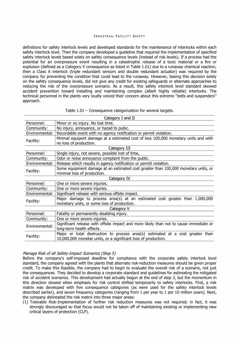
definitions for safety interlock levels and developed standards for the maintenance of interlocks within each safety interlock level. Then the company developed a guideline that required the implementation of specified safety interlock levels based solely on safety consequence levels (instead of risk levels). If a process had the potential for an overpressure event resulting in a catastrophic release of a toxic material or a fire or explosion (defined as a Category V consequence as listed in Table 1.01) due to a runaway chemical reaction, then a Class A interlock (triple redundant sensors and double redundant actuator) was required by the company for preventing the condition that could lead to the runaway. However, basing this decision solely on the safety consequence levels, did not give any credit for existing safeguards or alternate approaches to reducing the risk of the overpressure scenario. As a result, this safety interlock level standard skewed accident prevention toward installing and maintaining complex (albeit highly reliable) interlocks. The technical personnel in the plants very loudly voiced their concern about this extreme “belts and suspenders” approach.
Table 1.01 – Consequence categorization for several targets.
CCaatteeggoorryy II aanndd IIII Personnel: Minor or no injury. No lost time. Community: No injury, annoyance, or hazad to pubic. Environmental: Recordable event with no agency notification or permit violation.
Facility: Mnimal equipent damage at a estimeted cost of less 100,000 monetary units and with no loss of production.
CCaatteeggoorryy IIIIII Personnel: Single injury, not severe, possible lost of time, Community: Odor or noise annoyance complaint from the public. Environmental: Release which results in agency notification or permit violation.
Facility: Some equipment damage at an estimated cost greater than 100,000 monetary units, or minimal loss of production.
CCaatteeggoorryy IIVV Personnel: One or more severe injuries. Community: One or more severe injuries. Environmental: Significant release with serious offsite impact.
Facility: Major damage to process area(s) at an estimated cost greater than 1,000,000 monetary units, or some loss of production.
CCaatteeggoorryy VV Personnel: Fatality or permanently disabling injury. Community: One or more severe injuries.
Environmental: Significant release with offsite impact and more likely than not to cause immediate or long-term health effects.
Facility: Major or total destruction to process area(s) estimated at a cost greater than 10,000,000 monetar units, or a significant loss of production.
Manage Risk of all Safety-Impact Scenarios (Step 5) Before the company's self-imposed deadline for compliance with the corporate safety interlock level standard, the company agreed with the plants that alternate risk-reduction measures should be given proper credit. To make this feasible, the company had to begin to evaluate the overall risk of a scenario, not just the consequences. They decided to develop a corporate standard and guidelines for estimating the mitigated risk of accident scenarios. This development had actually begun at the end of step 3, but the momentum in this direction slowed when emphasis for risk control shifted temporarily to safety interlocks. First, a risk matrix was developed with five consequence categories (as were used for the safety interlock levels described earlier), and seven frequency categories (ranging from 1 per year to 1 per 10 million years). Next, the company delineated the risk matrix into three major areas: (1) Tolerable Risk-Implementation of further risk reduction measures was not required; in fact, it was
strongly discouraged so that focus would not be taken off of maintaining existing or implementing new critical layers of protection (CLP).

CC OO NN CC EE PP TT II OO NN ,, DD EE SS II GG NN ,, AA NN DD II MM PP LL EE MM EE NN TT AA TT II OO NN
(2) Intolerable Risk-Action was required to reduce the risk further. (3) Optional-An intermediate zone was defined, which allowed plant management the option to implement
further risk reduction measures, as they deemed necessary. Some companies would have called this a semi-quantitative approach, but in this company, the process hazard analyses (PHA) teams used this matrix to “qualitatively” judge risk. Teams would vote on which consequence and frequency categories an accident scenario belonged (considering the qualitative merits of each existing safeguard), and they would generate recommendations for scenarios not in the tolerable risk area. This approach worked well for most scenarios, but the company soon found considerable inconsistencies in the application of the risk matrix in qualitative risk judgments. Also, the company observed that too many accident scenarios were requiring resource-intensive quantitative risk assessments (QRA). It was clear that an intermediate approach for judging the risk of moderately complex scenarios was needed. And, the company still needed to eliminate the conflict between the risk matrix and the safety interlock level standard.
Table 1.02 – Consequence risk matrix and action categorization.
FFrreeqquueennccyy ooff CCoonnsseeqquueennccee
((ppeerr yyeeaarr)) CCaatteeggoorryy II CCaatteeggoorryy IIII CCaatteeggoorryy IIIIII CCaatteeggoorryy IIVV CCaatteeggoorryy VV
100 < f < 101 Optional (Eval. Alternatives)
Optional (Eval. Alternatives)
Notify Management Immediate Immediate
101 < f < 102 Optional (Eval. Alternatives)
Optional (Eval. Alternatives) Optional Notify
Management Immediate
102 < f < 103 Optional (Eval. Alternatives)
Optional (Eval. Alternatives)
Notify Management
Notify Management
Notify Management
103 < f < 104 No action Optional (Eval. Alternatives)
Optional (Eval. Alternatives)
Notify Management
Notify Management
104 < f < 105 No action No action Optional (Eval. Alternatives)
Optional (Eval. Alternatives)
Notify Management
105 < f < 106 No action No action No action Optional (Eval. Alternatives)
Optional (Eval. Alternatives)
106 < f < 107 No action No action No action No action Optional (Eval. Alternatives)
f < 107 No action No action No action No action No action Develop A Semiquantitative Approach (The Beginnings Of A Tiered Approach) For Risk Judgment (Step 6) This was a very significant step for the company to take; the effort began in early 1995 and was implemented in early 1996. Along with the inconsistencies in applying risk judgment tools, there was still confusion among plant personnel about when and how they should use the safety interlock level standard and the risk matrix. Both were useful tools that the company had spent considerable resources to develop and implement. The new guidelines would need to somehow integrate the safety interlock levels and the risk matrix categories to form a single standard for making decisions. And the plants also needed a tool (or multiple tools), besides the extremes of pure qualitative judgment and a quantitative risk assessments (QRA), to decide on the best alternative for controlling the risk of an identified scenario. The technical personnel from the corporate offices and from the plants worked together to develop a semiquantitative tool and to define the needed guidelines. One effort toward a semiquantitative tool involved defining a new term called an independent protection layer (IPL), which would represent a single layer of safety for an accident scenario. Defining this new term required developing examples of independent protection layers (IPL) to which the plant personnel would be able to relate. For example, a spring-loaded relief valve is independent from a high-pressure alarm; thus a system protected by both of these devices has two independent protection layers (IPL). On the other hand, a system protected by a high-pressure alarm and a shutdown interlock using the same transmitter has only one independent protection layer. Class A, Class B, and Class C safety interlocks (which were defined previously in the safety interlock level standard) were also included as

II NN DD UU SS TT RR II AA LL FF AA CC II LL II TT YY SS AA FF EE TT YY
example independent protection layers (IPL). To ensure consistent application of independent protection layers, i.e. to account for the relative reliability and availability of various types of independent protection layers, it was necessary to identify how much “credit” plant personnel could claim for a particular type of independent protection layer (IPL). For example, a Class A safety interlock would deserve more credit than a Class B interlock, and a relief valve would be given more credit than a process alarm. This need was addressed by assigning a “maximum credit number” for each example independent protection layers (see Table 1.03).
Table 1.03 – Credits for independent protection layers (IPL).
NNuummbbeerr ffoorr IInnddeeppeennddeenntt PPrrootteeccttiioonn LLaayyeerr ((IIPPLL)) EExxaammppllee IIPPLL BBaassiicc PPrroocceessss CCoonnttrrooll SSyysstteemm
Automatic control loop (if failure is not a significant initiating event contributor and is independent of the Class A, Class B, or Class C interlock, if applicable, and final element is tested at least once per 4 years).
1
HHuummaann IInntteerrvveennttiioonn Manual response in field with more than 10 minutes available for response (if sensor or alarm are independent of the Class A, Class B, or Class C interlock, if applicable, and operator training includes required response).
1
Manual response in field with more than 40 minutes available for response (if sensor or alarm are independent of the Class A, Class B, or Class C interlock, if applicable, and operator training includes required response).
2
PPaassssiivvee DDeevviicceess Secondary containment such as dike (if good administrative control over drain valves exists). 2
Spring-loaded relief valve in clean service. 3 SSaaffeettyy IInntteerrlloocckkss
Class A interlock (provided independent of other interlocks). 3 Class B interlock (provided independent of other interlocks). 2 Class C interlock (provided independent of other interlocks). 1
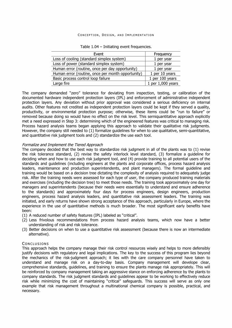
The credit is essentially the order of magnitude of the risk reduction anticipated by claiming the safeguard as an independent protection layer (IPL) for the accident scenario. The company believed that when process hazard analysis teams or designers used the independent protection layer definitions and related credit numbers, the consistency between risk analyses at the numerous plants would improve. Another (parallel) effort involved assigning frequency categories to typical “initiating events” for accident scenarios (see Table 1.04); these initiating events were intended to represent the types of events that could occur at any of the various plants. The frequency categories were derived from process hazard analysis (PHA) experience within the company and provided a consistent starting point for semiquantitative analysis. Finally, a semi-quantitative approach for estimating risk was developed, incorporating the frequency of initiating events and the independent protection layer (IPL) credits described previously. Although this approach used standard equations and calculation sheets not described here, the basic approach required teams to: (1) Identify the ultimate consequence of the accident scenario and document the scenario as clearly as
possible, stating the initiating event and any assumptions. (2) Estimate the frequency of the initiating event (using a frequency from Table 1.04, if possible). (3) Estimate the risk of the unmitigated event and determine from the risk matrix if the risk is tolerable as is
if the risk is not tolerable, take credit for existing independent protection layers (IPL) until the risk reaches a tolerable level in the risk matrix (use best judgment in defining independent protection layers and deciding which ones to take credit for first), and if the risk is still not tolerable, develop a recommendation(s) that will lower the risk to a tolerable level.
(4) Record the specific safety features (independent protection layers) that were used to reach a tolerable risk level.
CC OO NN CC EE PP TT II OO NN ,, DD EE SS II GG NN ,, AA NN DD II MM PP LL EE MM EE NN TT AA TT II OO NN
Table 1.04 – Initiating event frequencies.
EEvveenntt FFrreeqquueennccyy Loss of cooling (standard simplex system) 1 per year Loss of power (standard simplex system) 1 per year Human error (routine, once per day opportunity) 1 per year Human error (routine, once per month opportunity) 1 per 10 years Basic process control loop failure 1 per 100 years Large fire 1 per 1,000 years
The company demanded “zero” tolerance for deviating from inspection, testing, or calibration of the documented hardware independent protection layers (IPL) and enforcement of administrative independent protection layers. Any deviation without prior approval was considered a serious deficiency on internal audits. Other features not credited as independent protection layers could be kept if they served a quality, productivity, or environmental protection purpose; otherwise, these items could be “run to failure” or removed because doing so would have no effect on the risk level. This serniquantitative approach explicitly met a need expressed in Step 3: determining which of the engineered features was critical to managing risk. Process hazard analysis teams began applying this approach to validate their qualitative risk judgments. However, the company still needed to (1) formalize guidelines for when to use qualitative, semi-quantitative, and quantitative risk judgment tools and (2) standardize the use each tool. Formalize and Implement the Tiered Approach The company decided that the best way to standardize risk judgment in all of the plants was to (1) revise the risk tolerance standard, (2) revise the safety interlock level standard, (3) formalize a guideline for deciding when and how to use each risk judgment tool, and (4) provide training to all potential users of the standards and guidelines (including engineers at the plants and corporate offices, process hazard analysis leaders, maintenance and production superintendents, and plant managers). The formal guideline and training would be based on a decision tree dictating the complexity of analysis required to adequately judge risk. After the training needs were assessed for each type of user, the company produced training materials and exercises (including the decision tree) to meet those needs. The training took approximately one day for managers and superintendents (because their needs were essentially to understand and ensure adherence to the standards) and approximately four days for process engineers, design engineers, production engineers, process hazard analysis leaders, and quantitative risk assessment leaders. The training was initiated, and early returns have shown strong acceptance of this approach, particularly in Europe, where the experience in the use of quantitative methods is much broader. The most significant early benefits have been: (1) A reduced number of safety features (IPL) labeled as “critical”. (2) Less frivolous recommendations from process hazard analysis teams, which now have a better
understanding of risk and risk tolerance. (3) Better decisions on when to use a quantitative risk assessment (because there is now an intermediate
alternative). CC OO NN CC LL UU SS II OO NN SS This approach helps the company manage their risk control resources wisely and helps to more defensibly justify decisions with regulatory and legal implications. The key to the success of this program lies beyond the mechanics of the risk-judgment approach; it lies with the care company personnel have taken to understand and manage risk on a day-to-day basis. Company management will develope clear, comprehensive standards, guidelines, and training to ensure the plants manage risk appropriately. This will be reinforced by company management taking an aggressive stance on enforcing adherence by the plants to company standards. The risk judgment standards and guidelines appear to be working to effectively reduce risk while minimizing the cost of maintaining “critical” safeguards. This success will serve as only one example that risk management throughout a multinational chemical company is possible, practical, and necessary.

II NN DD UU SS TT RR II AA LL FF AA CC II LL II TT YY SS AA FF EE TT YY
RR EE FF EE RR EE NN CC EE SS Advanced Process Hazard Analysis Leader Training, Process Safety Institute, Knoxville, TN, 1993. D. F. Montague, Process Risk Evaluation-What Method to Use, Reliability Engineering and System Safety, Vol. 29, Elsevier Science Publishers Ltd., England, 1990. F. P. Lees, Loss Prevention in the Process Industries, Vols. 1 and 2, Butterworth's, London, 1980. Guidelines for Chemical Process Quantitative Risk Analysis, Center for Chemical Process Safety, American Institute of Chemical Engineers, New York, NY, 1989. Guidelines for Hazard Evaluation Procedures, 2nd Edition with Worked Examples, Center for Chemical Process Safety, American Institute of Chemical Engineers, New York, NY, 1992.
CC OO NN CC EE PP TT II OO NN ,, DD EE SS II GG NN ,, AA NN DD II MM PP LL EE MM EE NN TT AA TT II OO NN
CC HH AA PP TT EE RR 22
SSAAFFEETTYY LLVVEELL IINNTTEEGGRRIITTYY ((SSIILL))
BBAA CC KK GG RR OO UU NN DD In 1996, in response to an increasing number of industrial accidents, the Instrument Society of America (ISA) enacted a standard to drive the classification of safety instrumented systems for the process industry within the United States. This standard, ISA S84.01, introduced the concept of Safety Integrity Levels. Subsequently, the International Electrotechnical Commission (IEC) enacted an industry neutral standard, IEC 61508, to help quantify safety in programmable electronic safety-related systems. The combination of these standards has driven industry, most specifically the hydrocarbon processing and oil and gas industries, to seek instrumentation solutions that will improve the inherent safety of industry processes. As a byproduct, it was discovered that many of the parameters central to Safety Integrity Levels, once optimized, provided added reliability and up time for the concerned processes. This document will define and describe the key components of safety and reliability for instrumentation systems as well as draw contrasts between safety and reliability. Additionally, this document will briefly describe available methods for determining safety integrity levels. Lastly, a brief depiction of the governing standards will be presented.
WWHH AA TT AA RR EE SSAA FF EE TT YY II NN TT EE GG RR II TT YY LL EE VV EE LL SS ((SSII LL )) Safety integrity levels (SIL) are measures of the safety of a given process. Specifically, to what extent can the end user expect the process in question to perform safely, and in the case of a failure, fail in a safe manner? The specifics of this measurement are outlined in the standards IEC 61508, IEC 61511, JIS C 0508, and ISA SP84.01. It is important to note that no individual product can carry a safety integrity level rating. Individual components of processes, such as instrumentation, can only be certified for use within a given safety integrity level environment. The need to derive and associate safety integrity level values with processes is driven by risk based safety analysis (RBSA). Risk based safety analysis is the task of evaluating a process for safety risks, quantifying them, and subsequently categorizing them as acceptable or unacceptable. Acceptable risks are those that can be morally, monetarily, or otherwise, justified. Conversely, unacceptable risks are those whose consequences are too large or costly. However risks are justified, the goal is to arrive at a safe process. A typical risk based safety analysis might proceed as follows. With a desired level of safety being a starting point, a “risk budget” is established specifying the amount of risk of unsafe failure to be tolerated. The process can then be dissected into its functional components, with each being evaluated for risk. By combining these risk levels, a comparison of actual risk can be made against the risk budget. When actual risk outweighs budgeted risk, optimization is called for. Processes can be optimized for risk by selecting components rated for use within the desired safety integrity level environment. For example, if the desired safety integrity level value for the process is class SIL 3, then by using components rated for use within a safety integrity level environment this goal may be achieved. It is important to note that simply combining process components rated to be used in a given safety integrity level rated environment does not guarantee the process to be rated at the specified safety integrity level. The process safety integrity level must still be determined by an appropriate method. These are simplified calculations, fault tree analysis, or Markov analysis. An example of a tool used to estimate what safety integrity level rating to target for a given process is that of the risk assessment tree (RAT). See the Figure 2.05. By combining the appropriate parameters for a given process path, the risk assessment tree can be used to determine what safety integrity level value should be obtained. By optimizing certain process parameters, the SIL value of the process can be affected.

II NN DD UU SS TT RR II AA LL FF AA CC II LL II TT YY SS AA FF EE TT YY
SSAA FF EE YY LL II FF EE CC YY CC LL EE It is seldom, if ever, that an aspect of safety in any area of activity depends solely on one factor or on one piece of equipment. Thus the safety standards concerned here, IEC EN 61511 and IEC EN 61508, identify an overall approach to the task of determining and applying safety within a process plant. This approach, including the concept of a safety life cycle (SLC), directs the user to consider all of the required phases of the life cycle. In order to claim compliance with the standard it ensures that all issues are taken into account and fully documented for assessment. Essentially, the standards give the framework and direction for the application of the overall safety life cycle (SLC), covering all aspects of safety including conception, design, implementation, installation, commissioning, validation, maintenance and de-commissioning. The fact that “safety” and “life” are the key elements at the core of the standards should reinforce the purpose and scope of the documents. For the process industries the standard IEC EN 61511 provides relevant guidance for the user, including both hardware and software aspects of safety systems. To implement their strategies within these overall safety requirements the plant operators and designers of safety systems, following the directives of IEC EN 61511 for example, utilise equipment developed and validated according to IEC EN 61508 to achieve their safety instrumented systems (SIS). The standard IEC EN 61508 deals specifically with “functional safety of electrical, electronic, programmable electronic safety-related systems” and thus, for a manufacturer of process instrumentation interface equipment, the task is to develop and validate devices following the demands of IEC EN 61508 and to provide the relevant information to enable the use of these devices by others within their safety instrumented systems. Unlike previous fail-safe related standards in this field, IEC EN 61508 makes possible a “self-certification” approach for quantitative and qualitative safety-related assessments. To ensure that this is comprehensive and demonstrable to other parties it is obviously important that a common framework is adopted; this is where the safety life cycle can be seen to be of relevance. The safety life cycle, as shown in Figure 2.01, includes a series of steps and activities to be considered and implemented. Within the safety life cycle the various phases or steps may involve different personnel, groups, or even companies, to carry out the specific tasks. For example, the steps can be grouped together and the various responsibilities understood as identified below. The first five steps can be considered as an analytical group of activities: (1) Concept. (2) Overall scope definition. (3) Hazard and risk analysis. (4) Overall safety requirements. (5) Safety requirements allocation and would be carried out by the plant owner or end user, probably
working together with specialist consultants. The resulting outputs of overall definitions and requirements are the inputs to the next stages of activity.
Implementation measures The second group of implementation comprises the next eight steps: (1) Operation and maintenance planning. (2) Validation planning. (3) Installation and commissioning planning. (4) Safety-related systems and E/E/PES implementation. (5) Safety-related systems: other technology implementation. (6) External risk reduction facilities implementation. (7) Overall installation and commissioning. (8) Overall safety validation and would be conducted by the end user together with chosen contractors and
suppliers of equipment. It may be readily appreciated, that whilst each of these steps has a simple title, the work involved in carrying out the tasks can be complex and time-consuming!
The third group is essentially one of operating the process with its effective safeguards and involves the final three steps: (1) Overall operation and maintenance (2) Overall modification and retrofit (3) Decommissioning, these normally being carried out by the plant end-user and his contractors.

CC OO NN CC EE PP TT II OO NN ,, DD EE SS II GG NN ,, AA NN DD II MM PP LL EE MM EE NN TT AA TT II OO NN
Following the directives given in IEC EN 61511 and implementing the steps in the safety life cycle, when the safety assessments are carried out and E/E/PES are used to carry out safety functions, IEC EN 61508 then identifies the aspects which need to be addressed. There are essentially two groups, or types, of subsystems that are considered within the standard: (1) The equipment under control (EUC) carries out the required manufacturing or process activity. (2) The control and protection systems implement the safety functions necessary to ensure that the
equipment under control is suitably safe.
Overall operation andmaintenance planning
Concept
Overall ScopeDefinition
Hazard and RiskAnalysis
Overall SafetyRequirements
Safety RequirementsAllocation
Overall Planning Safety-related Systems(E/E/PES)
Safety-related Systems(other technology)
External RiskReduction Facilities
Overall safetyvalidation planning
Overall installation andcommissioning planning
Overall Installation andCommissioning
Overall SafetyValidation
Overall Operation andMmaintenance and
Repair
Decommissioning orDisposal
Overall Modificationand Retrofit
Back to appropriate overallsafety life cycle phase
Figure 2.01 – Phases of the safety life cycle. Fundamentally, the goal here is the achievement or maintenance of a safe state for the equipment under control. You can think of the “control system” causing a desired equipment under control operation and the

II NN DD UU SS TT RR II AA LL FF AA CC II LL II TT YY SS AA FF EE TT YY
“protection system” responding to undesired equipment under control operation. Note that, dependent upon the risk-reduction strategies implemented, it may be that some control functions are designated as safety functions. In other words, do not assume that all safety functions are to be performed by a separate protection system. If you find it difficult to conceive exactly what is meant by the IEC EN 61508 reference to equipment under control, it may be helpful to think in terms of “process”, which is the term used in IEC EN 61511. When any possible hazards are analysed and the risks arising from the equipment under control and its control system cannot be tolerated, then a way of reducing the risks to tolerable levels must be found. Perhaps in some cases the equipment under control or control system can be modified to achieve the requisite risk-reduction, but in other cases protection systems will be needed. These protection systems are designated safety-related systems, whose specific purpose is to mitigate the effects of a hazardous event or to prevent that event from occurring. RR II SS KK SS AA NN DD TT HH EE II RR RR EE DD UU CC TT II OO NN One phase of the safety life cycle (SLC) is the analysis of hazards and risks arising from the equipment under control and its control system. In the standards the concept of risk is defined as the probable rate of occurrence of a hazard (accident) causing harm and the degree of severity of harm. So risk can be seen as the product of “incident frequency” and “incident severity”. Often the consequences of an accident are implicit within the description of an accident, but if not they should be made explicit. There is a wide range of methods applied to the analysis of hazards and risk around the world and an overview is provided in both IEC EN 61511 and IEC EN 61508. These methods include techniques such as: (1) Hazard and Operability study (HAZOP). (2) Failure Mode Effect (and Criticality) Analysis (FMECA). (3) Failure Mode Effect and Diagnostics Analysis (FMEDA). (4) Event Tree Analysis (ETA). (5) Fault Tree Analysis (FTA). (6) Other study, checklist, graph and model methods. When there is a history of plant operating data or industry-specific methods or guidelines, then the analysis may be readily structured, but is still complex. This step of clearly identifying hazards and analysing risk is one of the most difficult to carry out, particularly if the process being studied is new or innovative. The standards embody the principle of balancing the risks associated with the equipment under control (i.e. the consequences and probability of hazardous events) by relevant dependable safety functions. This balance includes the aspect of tolerability of the risk. For example, the probable occurrence of a hazard whose consequence is negligible could be considered tolerable, whereas even the occasional occurrence of a catastrophe would be an intolerable risk. If, in order to achieve the required level of safety, the risks of the equipment under control cannot be tolerated according to the criteria established, then safety functions must be implemented to reduce the risk. The goal is to ensure that the residual risk – the probability of a hazardous event occurring even with the safety functions in place – is less than or equal to the tolerable risk. The diagram shows this effectively, where the risk posed by the equipment under control is reduced to a tolerable level by a “necessary risk reduction” strategy. The reduction of risk can be achieved by a combination of items rather than depending upon only one safety system and can comprise organisational measures as well. The effect of these risk reduction measures and systems must be to achieve an “actual risk reduction” that is greater than or equal to the necessary risk reduction.
SSAA FF EE TT YY II NN TT EE GG RR II TT YY LL EE VV EE LL FFUU NN DD AA MM EE NN TT AA LL SS As we have seen, analysis of hazards and risks gives rise to the need to reduce the risk and within the safety life cycle (SLC) of the standards this is identified as the derivation of the safety requirements. There may be some overall methods and mechanisms described in the safety requirements but also these requirements are then broken down into specific safety functions to achieve a defined task. In parallel with this allocation of the overall safety requirements to specific safety functions, a measure of the dependability or integrity of those safety functions is required. What is the confidence that the safety function will perform when called upon? This measure is the safety integrity level (SIL). More precisely, the safety integrity of a system can be defined as “the probability (likelihood) of a safety-related system performing the required safety function

CC OO NN CC EE PP TT II OO NN ,, DD EE SS II GG NN ,, AA NN DD II MM PP LL EE MM EE NN TT AA TT II OO NN
under all the stated conditions within a stated period of time”. Thus the specification of the safety function includes both the actions to be taken in response to the existence of particular conditions and also the time for that response to take place. The safety integrity level is a measure of the reliability of the safety function performing to specification. PP RR OO BB AA BB II LL II TT YY OO FF FF AA II LL UU RR EE To categorise the safety integrity of a safety function the probability of failure is considered, in effect the inverse of the safety integrity level definition, looking at failure to perform rather than success. It is easier to identify and quantify possible conditions and causes leading to failure of a safety function than it is to guarantee the desired action of a safety function when called upon. Two classes of safety integrity level are identified, depending on the service provided by the safety function. For safety functions that are activated when required (on demand mode) the probability of failure to perform correctly is given, whilst for safety functions that are in place continuously the probability of a dangerous failure is expressed in terms of a given period of time (per hour or in continous mode). In summary, IEC EN 61508 requires that when safety functions are to be performed by E/E/PES the safety integrity is specified in terms of a safety integrity level. The probabilities of failure are related to one of four safety integrity levels, as shown in Table 2.01.
Table 2.01 – Probability of failure.
MMooddee ooff OOppeerraattiioonn ((PPrroobbaabbiilliittyy ooff FFaaiilluurree)) SSIILL OOnn DDeemmaanndd CCoonnttiinnuuoouuss ((ppeerr hhoouurr))
4 105 P < 104 109 P < 108 3 104 P < 103 108 P < 107 2 103 P < 102 107 P < 106 1 102 P < 101 106 P < 105
An important consideration for any safety related system or equipment is the level of certainty that the required safe response or action will take place when it is needed. This is normally determined as the likelihood that the safety loop will fail to act as and when it is required to and is expressed as a probability. The standards apply both to safety systems operating on demand, such as an emergency shut-down (ESD) system, and to systems operating “continuously” or in high demand, such as the process control system. For a safety loop operating in the demand mode of operation the relevant factor is the probability the function fails on demand average (PFDavg), which is the average probability of failure on demand. For a continuous or high demand mode of operation the probability of a dangerous failure per hour (PFH) is considered rather than probability the function fails on demand average (PFDavg). Obviously the aspect of risk that was discussed earlier and the probability of failure on demand of a safety function are closely related. Using the definitions, frequency of accident or event in the absence of protection functions (Fnp) and tolerable frequency of accident or event (Ft), then the risk reduction factor (R) is defined as,
t
np
F
FR [2.01]
whereas probability the function fails on demand (PFD) is the inverse,
np
tavg F
FR1
PFD
[2.02]
Since the concepts are closely linked, similar methods and tools are used to evaluate risk and to assess the probability the function fails on demand average (PFDavg). Failure modes and effects analysis (FMEA) is a way to document the system being considered using a systematic approach to identify and evaluate the effects of component failures and to determine what could reduce or eliminate the chance of failure. Once the possible failures and their consequence have been evaluated, the various operational states of the subsystem can be associated using the Markov models, for example. One other factor that needs to be applied to the calculation is that of the interval between tests, which is known as the “proof time” or the

II NN DD UU SS TT RR II AA LL FF AA CC II LL II TT YY SS AA FF EE TT YY
“proof test interval”. This is a variable that may depend not only upon the practical implementation of testing and maintenance within the system, subsystem or component concerned, but also upon the desired end result. By varying the proof time within the model it can result that the subsystem or safety loop may be suitable for use with a different safety integrity level (SIL). Practical and operational considerations are often the guide. In the related area of application that most readers may be familiar with one can consider the fire alarm system in a commercial premises. Here, the legal or insurance driven need to frequently test the system must be balanced with the practicality and cost to organise the tests. Maybe the insurance premiums would be lower if the system were to be tested more frequently but the cost and disruption to organise and implement them may not be worth it. Note also that “low demand mode” is defined as one where the frequency of demands for operation made on a safety related system is no greater than one per year and no greater than twice the proof test frequency. Failure rate d is the dangerous (detected and undetected) failure rate of a channel in a subsystem. For the probability the function fails on demand (PFD) calculation (low demand mode) it is stated as failures per year. Target failure measure probability the function fails on demand average (PFDavg) is the average probability of failure on demand of a safety function or subsystem, also called average probability of failure on demand. The probability of a failure is time dependant,
dte1tQ [2.03] It is a function of the failure rate () and the time (t) between proof tests. The maximum safety integrity level (SIL) according to the failure probability requirements is then read out from Table 2.05. That means that you cannot find out the maximum safety integrity level of your system, or subsystem, if you do not know if a test procedure is implemented by the user and what the test intervals are! These values are required for the whole safety function, usually including different systems or subsystems. The average probability of failure on demand of a safety function is determined by calculating and combining the average probability of failure on demand for all the subsystems, which together provide the safety function. If the probabilities are small, this can be expressed by the following,
PFDsys = PFDs + PFDl + PFDfe [2.04] where PFDsys is the average probability of failure on demand of a safety function safety-related system; PFDs is the average probability of failure on demand for the sensor subsystem; PFDl is the average probability of failure on demand for the logic subsystem; and, PFDfe is the average probability of failure on demand for the final element subsystem. TT HH EE SS YY SS TT EE MM SS TT RR UU CC TT UU RR EE The safe failure fraction (SFF) is the fraction of the total failures that are assessed as either safe or diagnosed or detected. When analysing the various failure states and failure modes of components they can be categorised and grouped according to their effect on the safety of the device. Thus we have the terms: (1) safe is the failure rate of components leading to a safe state. (2) dangerous is a failure rate of components leading to a potentially dangerous state. These terms are further categorised into “detected” or “undetected” to reflect the level of diagnostic ability within the device. For example: (1) dd is dangerous detected failure rate (2) du is dangerous undetected failure rate. The sum of all the component failure rates is expressed as,
dangeroussafetotal [2.05]
and the safe failure fraction (SFF) can be calculated as,
total
du1SFF [2.06]

CC OO NN CC EE PP TT II OO NN ,, DD EE SS II GG NN ,, AA NN DD II MM PP LL EE MM EE NN TT AA TT II OO NN
Hardware Fault Tolerance One further complication in associating the safe failure fraction (SFF) with a safety integrity level (SIL) is that when considering hardware safety integrity two types of subsystems are defined. For type A subsystems it is considered that all possible failure modes can be determined for all elements, while for type B subsystems it is considered that it is not possible to completely determine the behaviour under fault conditions. Subsystem type A have by definition a set of characteristics: the failure mode of all components well defined, and behaviour of the subsystem under fault conditions can be completely determined, and sufficient dependable failure data from field experience show that the claimed rates of failure for detected and undetected dangerous failures are met. Table 2.02 – Hardware safety integrity. Architectural constraints on type A safety-related subsystems (IEC EN 61508-2, Part 2).
SSaaffeettyy FFaaiilluurree FFrraaccttiioonn HHaarrddwwaarree FFaauulltt TToolleerraannccee ((HHFFTT)) ((SSFFFF)) 00 11 22
< 60% SIL 1 SIL 2 SIL 3 60% 90% SIL 2 SIL 3 SIL 4 90% 99% SIL 3 SIL 4 SIL 4
> 99% SIL 3 SIL 4 SIL 4 Subsystem type B have by definition the characteristics: the failure mode of at least one component is not well defined, or behaviour of the subsystem under fault conditions cannot be completely determined, or insufficient dependable failure data from field experience show that the claimed rates of failure for detected and undetected dangerous failures are met. Table 2.03 – Hardware safety integrity. Architectural constraints on type B safety-related subsystems (IEC EN 61508-2, part 3).
SSaaffeettyy FFaaiilluurree FFrraaccttiioonn HHaarrddwwaarree FFaauulltt TToolleerraannccee ((HHFFTT)) ((SSFFFF)) 00 11 22
< 60% Not allowed SIL 1 SIL 2 60% 90% SIL 1 SIL 2 SIL 3 90% 99% SIL 2 SIL 3 SIL 4
> 99% SIL 3 SIL 4 SIL 4 These definitions, in combination with the fault tolerance of the hardware, are part of the “architectural constraints” for the hardware safety integrity as shown in Table 2.02 and Table 2.03. In the tables above, a hardware fault tolerance of N means that N+1 faults could cause a loss of the safety function. For example, if a subsystem has a hardware fault tolerance of 1 then 2 faults need to occur before the safety function is lost. We have seen that protection functions, whether performed within the control system or a separate protection system, are referred to as safetyrelated systems. If, after analysis of possible hazards arising from the equipment under control (EUC) and its control system, it is decided that there is no need to designate any safety functions, then one of the requirements of IEC EN 61508 is that the dangerous failure rate of the equipment under control system shall be below the levels given as SIL 1 rating. So, even when a process may be considered as benign, with no intolerable risks, the control system must be shown to have a rate not lower than 105 dangerous failures per hour. Connecting Risk and Safety Integrity Level Already we have briefly met the concepts of risk, the need to reduce these risks by safety functions and the requirement for integrity of these safety functions. One of the problems faced by process owners and users is how to associate the relevant safety integrity level with the safety function that is being applied to balance a particular risk. The risk graph shown in the Figure 2.02, based upon IEC EN 61508, is a way of achieving the linkage between the risk parameters and the safety integrity level for the safety function. For example, with the particular process being studied, the low or rare probability of minor injury is considered a tolerable risk, whilst if it is highly probable that there is frequent risk of serious injury then the safety function to reduce that risk would require an integrity level of three. There are two further concepts related to the
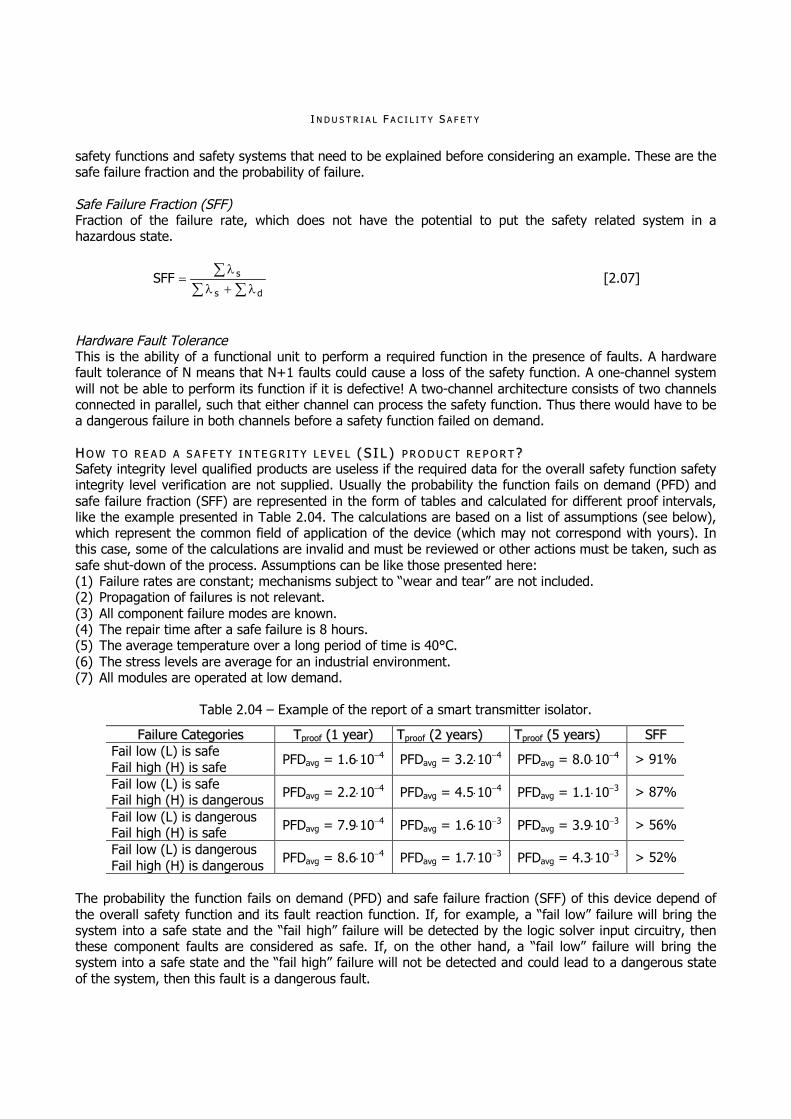
II NN DD UU SS TT RR II AA LL FF AA CC II LL II TT YY SS AA FF EE TT YY
safety functions and safety systems that need to be explained before considering an example. These are the safe failure fraction and the probability of failure. Safe Failure Fraction (SFF) Fraction of the failure rate, which does not have the potential to put the safety related system in a hazardous state.
ds
sSFF [2.07]
Hardware Fault Tolerance This is the ability of a functional unit to perform a required function in the presence of faults. A hardware fault tolerance of N means that N+1 faults could cause a loss of the safety function. A one-channel system will not be able to perform its function if it is defective! A two-channel architecture consists of two channels connected in parallel, such that either channel can process the safety function. Thus there would have to be a dangerous failure in both channels before a safety function failed on demand. HH OO WW TT OO RR EE AA DD AA SS AA FF EE TT YY II NN TT EE GG RR II TT YY LL EE VV EE LL (( SS II LL )) PP RR OO DD UU CC TT RR EE PP OO RR TT ?? Safety integrity level qualified products are useless if the required data for the overall safety function safety integrity level verification are not supplied. Usually the probability the function fails on demand (PFD) and safe failure fraction (SFF) are represented in the form of tables and calculated for different proof intervals, like the example presented in Table 2.04. The calculations are based on a list of assumptions (see below), which represent the common field of application of the device (which may not correspond with yours). In this case, some of the calculations are invalid and must be reviewed or other actions must be taken, such as safe shut-down of the process. Assumptions can be like those presented here: (1) Failure rates are constant; mechanisms subject to “wear and tear” are not included. (2) Propagation of failures is not relevant. (3) All component failure modes are known. (4) The repair time after a safe failure is 8 hours. (5) The average temperature over a long period of time is 40°C. (6) The stress levels are average for an industrial environment. (7) All modules are operated at low demand.
Table 2.04 – Example of the report of a smart transmitter isolator.
FFaaiilluurree CCaatteeggoorriieess TTpprrooooff ((11 yyeeaarr)) TTpprrooooff ((22 yyeeaarrss)) TTpprrooooff ((55 yyeeaarrss)) SSFFFF Fail low (L) is safe Fail high (H) is safe PFDavg = 1.6104 PFDavg = 3.2104 PFDavg = 8.0104 > 91%
Fail low (L) is safe Fail high (H) is dangerous PFDavg = 2.2104 PFDavg = 4.5104 PFDavg = 1.1103 > 87%
Fail low (L) is dangerous Fail high (H) is safe PFDavg = 7.9104 PFDavg = 1.6103 PFDavg = 3.9103 > 56%
Fail low (L) is dangerous Fail high (H) is dangerous PFDavg = 8.6104 PFDavg = 1.7103 PFDavg = 4.3103 > 52%
The probability the function fails on demand (PFD) and safe failure fraction (SFF) of this device depend of the overall safety function and its fault reaction function. If, for example, a “fail low” failure will bring the system into a safe state and the “fail high” failure will be detected by the logic solver input circuitry, then these component faults are considered as safe. If, on the other hand, a “fail low” failure will bring the system into a safe state and the “fail high” failure will not be detected and could lead to a dangerous state of the system, then this fault is a dangerous fault.

CC OO NN CC EE PP TT II OO NN ,, DD EE SS II GG NN ,, AA NN DD II MM PP LL EE MM EE NN TT AA TT II OO NN
SS AA FF EE TT YY II NN TT EE GG RR II TT YY LL EE VV EE LL FF OO RR MM UU LL AA EE The failure rate is expressed as the number of failures per unit of time for a given number of components (Ncomp), ususally stated in failures per billion hours (FIT, 109 hours).
compNFIT
[2.08]
Usually, the failure rate of components and systems is high at the beginning of their life and falls rapidly (“infant mortality”, defective components fail normally within 72 hours). Then, for a long time period the failure rate is constant. At the end of their life, the failure rate of components and systems starts to increase, due to wear effects. This failure distribution is also referred to as a “bathtub” curve. In the area of electrical and electronic devices the failure rate is considered to be constant ( = k). Since we have considered the failure rate as being constant, in this case the failure distribution will be exponential. This kind of probability density function (PDF) is very common in the technical field.
tetf [2.09] where is the constant failure rate (failures per unit of time) and t is the time. The cumulative distribution function (CDF, also referred to as the cumulative density function) represents the cumulated probability of a random component failure, F(t). F(t) is also referred to as the unavailability and includes all the failure modes. The probability of failure on demand (PFD) is given by,
PDF = F(t) – PFS [2.10] where PFS is the probability of safe failures, PFD is the probability of dangerous failures ( = du), and F(t) is the probability of failure on demand (PFD), when = du. For continuous random variable,
t
dttftF [2.11]
where f(t) is the probability density function (PDF). In the case of an exponential distribution,
te1tF [2.12] If t is much lower than 1, then we can assume that,
ttF [2.13] Accordingly, the reliability is given by,
tetR [2.14] The reliability represents the probability that a component will operate successfully. The only parameter of interest in industrial control systems, in this context, is the average probability of failure on demand (PFDavg). In the case of an exponential distribution,
1T
01avg dttF
T1
PFD [2.15]
If t is much lower than 1, then we have the following,

II NN DD UU SS TT RR II AA LL FF AA CC II LL II TT YY SS AA FF EE TT YY
1T
0d
1avg dtt
T1
PFD [2.16]
where d is the rate of dangerous failures per unit of time and T1 is the time to the next test.
1davg T21
PFD [2.17]
If the relationship between du and dd is unknown, one usually sets the following assumption,
1d T21
PFD [2.18]
and
1davg T41
PFD [2.19]
where du are the dangerous undetected failures and dd are the dangerous detected failures. The mean time between failures (MTBF) is the “expected” time to a failure and not the “guaranteed minimum life time”! For constant failure rates,
T
0dttRMTBF [2.20]
or
1MTBF [2.21]
MM EE TT HH OO DD SS OO FF DDEE TT EE RR MM II NN II NN GG SSAA FF EE TT YY II NN TT EE GG RR II TT YY LL EE VV EE LL RR EE QQ UU II RR EE MM EE NN TT SS The concept of safety integrity levels (SIL) was introduced during the development of BS EN 61508 (BSI 2002) as a measure of the quality or dependability of a system which has a safety function – a measure of the confidence with which the system can be expected to perform that function. It is also used in BS IEC 61511 (BSI 2003), the process sector specific application of BS EN 61508. This chapter discusses the application of two popular methods of determining safety integrity levels requirements – risk graph methods and layer of protection analysis (LOPA) – to process industry installations. It identifies some of the advantages of both methods, but also outlines some limitations, particularly of the risk graph method. It suggests criteria for identifying the situations where the use of these methods is appropriate. DD EE FF II NN II TT II OO NN SS OO FF SS AA FF EE TT YY II NN TT EE GG RR II TT YY LL EE VV EE LL SS The standards recognise that safety functions can be required to operate in quite different ways. In particular they recognise that many such functions are only called upon at a low frequency (these functions have a low demand rate). If we consider a car, examples of such functions applied to the car are: (1) Anti-lock braking (ABS). It depends on the driver, of course! (2) Secondary restraint system (SRS), such air bags. On the other hand there are functions which are in frequent or continuous use; examples of such functions are: (1) Normal braking. (2) Steering.

CC OO NN CC EE PP TT II OO NN ,, DD EE SS II GG NN ,, AA NN DD II MM PP LL EE MM EE NN TT AA TT II OO NN
The fundamental question is how frequently will failures of either type of function lead to accidents. The answer is different for the two types: (1) For functions with a low demand rate, the accident rate is a combination of two parameters. The first
parameter is the frequency of demands, and the second parameter is the probability the function fails on demand (PFD). In this case, therefore, the appropriate measure of performance of the function is function fails on demand, or its reciprocal, risk reduction factor (RRF).
(2) For functions which have a high demand rate or operate continuously, the accident rate is the failure rate () which is the appropriate measure of performance. An alternative measure is mean time to failure (MTTF) of the function. Provided failures are exponentially distributed, mean time to failure is the reciprocal of failure rate ().
These performance measures are, of course, related. At its simplest, provided the function can be proof-tested at a frequency which is greater than the demand rate, the relationship can be expressed as,
MTTF2t
2t
PFD
[2.22]
or
tMTTF2
t2
RRF
[2.23]
where t is the proof-test interval. Note that to significantly reduce the accident rate below the failure rate
of the function, the test frequency
t1
, should be at least two and preferably equal to five times the
demand frequency. They are, however, different quantities. Probability the function fails on demand (PFD) is a probability (dimensionless); is a failure rate with dimension units time1. The standards, however, use the same term safety integrity level (SIL) for both these measures, with the following definitions shown in the Table 2.05. Table 2.05 – Definitions of safety integrity level (SIL) for low demand mode and high demand mode (BS EN 61508).
LLooww DDeemmaanndd MMooddee SSIILL PPFFDD RRRRFF 4 10-5 PFD < 10-4 100,000 RRF > 10,000 3 10-4 PFD < 10-3 10,000 RRF > 1,000 2 10-3 PFD < 10-2 1,000 RRF > 100 1 10-2 PFD < 10-1 100 RRF > 10
HHiigghh DDeemmaanndd MMooddee // CCoonnttiinnuuoouuss MMooddee SSIILL ((hhrr11)) MMTTTTFF ((yyeeaarrss)) 4 10-9 < 10-8 100,000 MTTF > 10,000 3 10-8 < 10-7 10,000 MTTF > 1,000 2 10-7 < 10-6 1,000 MTTF > 100 1 10-6 < 10-5 100 MTTF > 10
In low demand mode, safety integrity level (SIL) is a proxy for probability the function fails on demand (PFD); in high demand and continuous mode, safety integrity level is a proxy for failure rate. The boundary between low demand mode and high demand mode is in essence set in the standards at one demand per year. This is consistent with proof-test intervals of 3 to 6 months, which in many cases will be the shortest feasible interval. Now consider a function which protects against two different hazards, one of which occurs at a rate of 1 every 2 weeks, or 25 times per year, i.e. a high demand rate, and the other at a rate of 1 in 10 years, i.e. a low demand rate. If the mean time to failure (MTTF) of the function is 50 years, it would qualify

II NN DD UU SS TT RR II AA LL FF AA CC II LL II TT YY SS AA FF EE TT YY
as achieving SIL 1 rating for the high demand rate hazard. The high demands effectively proof-test the function against the low demand rate hazard. All else being equal, the effective safety integrity level for the second hazard is given by,
410450204.0
PFD
SIL 3 rating [2.24]
So what is the safety integrity level achieved by the function? Clearly it is not unique, but depends on the hazard and in particular whether the demand rate for the hazard implies low or high demand mode. In the first case, the achievable safety integrity level is intrinsic to the equipment; in the second case, although the intrinsic quality of the equipment is important, the achievable safety integrity level is also affected by the testing regime. This is important in the process industry sector, where achievable safety integrity levels are liable to be dominated by the reliability of field equipment – process measurement instruments and, particularly, final elements such as shutdown valves – which need to be regularly tested to achieve required safety integrity levels. The differences between these definitions may be well understood by those who are dealing with the standards day-by-day, but are potentially confusing to those who only use them intermittently. The standard BS EN 61508 offers three methods of determining safety integrity level requirements: (1) Quantitative method. (2) Risk graph, described in the standard as a qualitative method. (3) Hazardous event severity matrix, also described as a qualitative method. Additionally, BS IEC 61511 offers: (1) Semi-quantitative method. (2) Safety layer matrix method, described as a semi-qualitative method. (3) Calibrated risk graph, described in the standard as a semi-qualitative method, but by some practitioners
as a semi-quantitative method. (4) Risk graph, described as a qualitative method. (5) Layer of protection analysis (LOPA). Although the standard does not assign this method a position on
the qualitative and quantitative scale, it is weighted toward the quantitative end. Risk graphs and layer of protection analysis are popular methods for determining safety integrity level requirements, particularly in the process industry sector. Their advantages and disadvantages and range of applicability are the main topic of this chapter. RR II SS KK GG RR AA PP HH II CC MM EE TT HH OO DD SS Risk graph methods are widely used for reasons outlined below. A typical risk graph is shown in Figure 2.02. The parameters of the risk graph can be given qualitative descriptions, e.g. CC is death of several persons, or quantitative descriptions, e.g. CC is probable fatalities per event in range 0.1 to 1.0. The first definition begs the question “What does several mean?”. In practice it is likely to be very difficult to assess safety integrity level requirements unless there is a set of agreed definitions of the parameter values, almost inevitably in terms of quantitative ranges. These may or may not have been calibrated against the assessing organisation’s risk criteria, but the method then becomes semi-quantitative (or is it semi-qualitative?). It is certainly somewhere between the extremities of the qualitative and quantitative scale. Table 2.06 shows a typical set of definitions. Benefits of Risk Graphic Methods Risk graph methods have the following advantages: (1) They are semi-qualitative or semi-quantitative. Precise hazard rates, consequences, and values for the
other parameters of the method, are not required; no specialist calculations or complex modelling is required. They can be applied by people with a good “feel” for the application domain.
(2) They are normally applied as a team exercise, similar to Hazard and Operability Analysis (HAZOP). Individual bias can be avoided; understanding about hazards and risks is disseminated among team members (e.g. from design, operations, and maintenance); issues are flushed out which may not be apparent to an individual. Planning and discipline are required.
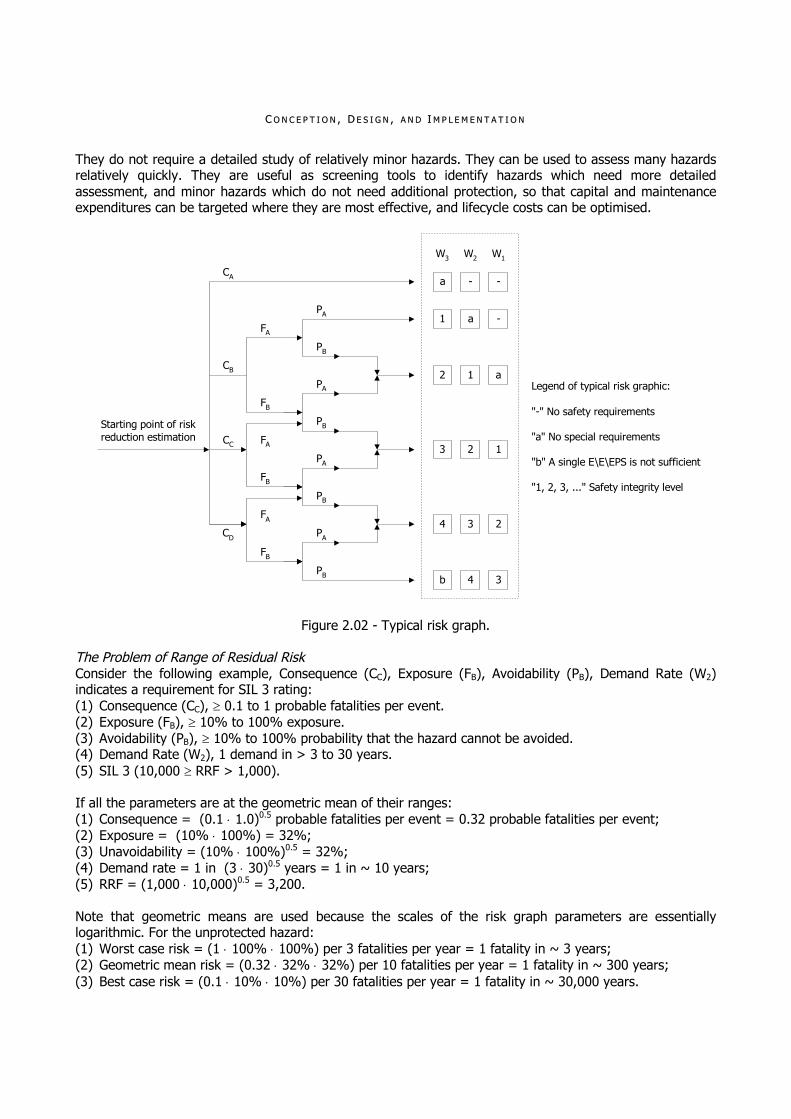
CC OO NN CC EE PP TT II OO NN ,, DD EE SS II GG NN ,, AA NN DD II MM PP LL EE MM EE NN TT AA TT II OO NN
They do not require a detailed study of relatively minor hazards. They can be used to assess many hazards relatively quickly. They are useful as screening tools to identify hazards which need more detailed assessment, and minor hazards which do not need additional protection, so that capital and maintenance expenditures can be targeted where they are most effective, and lifecycle costs can be optimised.
Starting point of riskreduction estimation
CA
CB
CC
CD
FA
FB
FA
FB
PA
PB
PA
PB
PA
PB
PA
PB
FA
FB
a - -
1 a -
2 1 a
3 2 1
4 3 2
b 4 3
W3 W2 W1
Legend of typical risk graphic:
"-" No safety requirements
"a" No special requirements
"b" A single E\E\EPS is not sufficient
"1, 2, 3, ..." Safety integrity level
Figure 2.02 - Typical risk graph. The Problem of Range of Residual Risk Consider the following example, Consequence (CC), Exposure (FB), Avoidability (PB), Demand Rate (W2) indicates a requirement for SIL 3 rating: (1) Consequence (CC), 0.1 to 1 probable fatalities per event. (2) Exposure (FB), 10% to 100% exposure. (3) Avoidability (PB), 10% to 100% probability that the hazard cannot be avoided. (4) Demand Rate (W2), 1 demand in > 3 to 30 years. (5) SIL 3 (10,000 RRF > 1,000). If all the parameters are at the geometric mean of their ranges: (1) Consequence = (0.1 1.0)0.5 probable fatalities per event = 0.32 probable fatalities per event; (2) Exposure = (10% 100%) = 32%; (3) Unavoidability = (10% 100%)0.5 = 32%; (4) Demand rate = 1 in (3 30)0.5 years = 1 in ~ 10 years; (5) RRF = (1,000 10,000)0.5 = 3,200. Note that geometric means are used because the scales of the risk graph parameters are essentially logarithmic. For the unprotected hazard: (1) Worst case risk = (1 100% 100%) per 3 fatalities per year = 1 fatality in ~ 3 years; (2) Geometric mean risk = (0.32 32% 32%) per 10 fatalities per year = 1 fatality in ~ 300 years; (3) Best case risk = (0.1 10% 10%) per 30 fatalities per year = 1 fatality in ~ 30,000 years.

II NN DD UU SS TT RR II AA LL FF AA CC II LL II TT YY SS AA FF EE TT YY
Table 2.06 – Typical definitions of risk graph parameters.
CCoonnsseeqquueennccee CCllaassss CCoonnssqquueennccee CA Minor injury CB 0.01 to 0.1 probable fatalities per event CC > 0.1 to 1.0 probable fatalities per event CD > 1 probable fatalities per event
EExxppoossuurree CCllaassss EExxppoossuurree FA < 10% of time FB 10% of time
AAvvooiiddaabbiilliittyy CCllaassss AAvvooiiddaabbiilliittyy UUnnaavvooiiddaabbiilliittyy
PA > 90% probability of avoiding hazard
< 10% probability hazard cannot be avoided
PB 90% probability of avoiding hazard
10% probability hazard cannot be avoided
DDeemmaanndd RRaattee CCllaassss DDeemmaanndd RRaattee W1 < 1 in 30 years W2 1 in > 3 to 30 years W3 1 in > 0.3 to 3 years
Conclusion, the unprotected risk has a range of 4 orders of magnitude. With SIL 3 rating protection: (1) Worst case residual risk = 1 fatality in (~ 3 1,000) years = 1 fatality in ~ 3,000 years; (2) Geometric mean residual risk = 1 fatality in (~ 300 3,200) years = 1 fatality in ~ 1 million years; (3) Best case residual risk = 1 fatality in (~ 30,000 10,000) years = 1 fatality in ~ 300 million years. With SIL 3 rating the residual risk with protection has a range of 5 orders of magnitude. Figure 2.03 shows the principle, based on the mean case.
Residual Risk Tolerable Risk Process Risk
One fatality in1,000,000 years
One fatality in100,000 years
One fatality in300 years
Increasing Risk
Necessary Risk Reduction
Actual Risk Reduction
Partial risk covered byother protection layers
Partial riskcovered by SIS
Partial risk covered by other non-SIS prevention and mitigation
protection layers
Risk reduction achieved by all protection layers
Figure 2.03 – Risk reduction model from BS IEC 61511. A reasonable target for this single hazard might be 1 fatality in 100,000 years. In the worst case we achieve less risk reduction than required by a factor of 30; in the mean case we achieve more risk reduction than required by a factor of 10; and in the best case we achieve more risk reduction than required by a factor of 3,000. In practice, of course, it is most unlikely that all the parameters will be at their extreme values, but on average the method must yield conservative results to avoid any significant probability that the required

CC OO NN CC EE PP TT II OO NN ,, DD EE SS II GG NN ,, AA NN DD II MM PP LL EE MM EE NN TT AA TT II OO NN
risk reduction is under-estimated. Ways of managing the inherent uncertainty in the range of residual risk, to produce a conservative outcome, include: (1) Calibrating the graph so that the mean residual risk is significantly below the target, as above. (2) Selecting the parameter values cautiously, i.e. by tending to select the more onerous range whenever
there is any uncertainty about which value is appropriate. Restricting the use of the method to situations where the mean residual risk from any single hazard is only a very small proportion of the overall total target risk. If there are a number of hazards protected by different systems or functions, the total mean residual risk from these hazards should only be a small proportion of the overall total target risk. It is then very likely that an under-estimate of the residual risk from one hazard will still be a small fraction of the overall target risk, and will be compensated by an over-estimate for another hazard when the risks are aggregated.
This conservatism may incur a substantial financial penalty, particularly if higher safety integrity level requirements are assessed. Use in the Process Industries Risk graphs are popular in the process industries for the assessment of the variety of trip functions – high and low pressure, temperature, level and flow, and so on – which are found in the average process plant. In this application domain, the benefits listed above are relevant, and the criterion that there are a number of functions whose risks can be aggregated is usually satisfied. The objective is to assess the safety integrity level requirement of the instrumented overpressure trip function, in the terminology of BS IEC 61511, a “safety instrumented function” (SIF) implemented by a “safety instrumented system” (SIS). One issue which arises immediately, when applying a typical risk graph in a case such as this, is how to account for the relief valve, which also protects the vessel from overpressure. This is a common situation, a safety instrumented function backed up mechanical protection. The options are: (1) Assume it ALWAYS works. (2) Assume it NEVER works. (3) Something in-between. The first option was recommended in the UKOOA Guidelines (UKOOA, 1999), but cannot be justified from failure rate data. The second option is liable to lead to an over-estimate of the required SIL, and to incur a cost penalty, so cannot be recommended. An approach which has been found to work, and which accords with the standards is: (1) Derive an overall risk reduction requirement (SIL) on the basis that there is no protection, i.e. before
applying the safety instrumented function (SIF) or any mechanical protection. (2) Take credit for the mechanical device, usually as equivalent to SIL 2 rating for a relief valve (this is
justified by available failure rate data, and is also supported by BS IEC 61511, Part 3, Annex F). (3) The required safety integrity level (SIL) for the safety instrumented function is the safety integrity level
determined in the first step minus 2 (or the equivalent safety integrity level of the mechanical protection).
The advantages of this approach are: (1) It produces results which are generally consistent with conventional practice. (2) It does not assume that mechanical devices are either perfect or useless. (3) It recognises that safety instrumented functions (SIF) require a safety integrity level (SIL) whenever the
overall requirement exceeds the equivalent safety integrity level of the mechanical device (e.g. overall requirement must have a SIL 3 rating; relief valve must have SIL 2 rating; safety instrumented function requirement must have SIL 1 rating).
General Calibration for Process Plants Before a risk graph can be calibrated, it must first be decided whether the basis will be: (1) Individual risk (IR), usually of someone identified as the most exposed individual. (2) Group risk of an exposed population group, such as the workers on the plant or the members of the
public on a nearby housing estate.

II NN DD UU SS TT RR II AA LL FF AA CC II LL II TT YY SS AA FF EE TT YY
(3) Some combination of these two types of risk. Calibration for Process Plants Based on Group Risk Consider the risk graph and definitions developed above as they might be applied to the group risk of the workers on a given plant. If we assume that on the plant there are twenty such functions, then, based on the geometric mean residual risk (1 in 1 million years), the total risk is 1 fatality in 50,000 years. Compare this figure with published criteria for the acceptability of risks. The United Kingdom Health and Safety and Environment Protection Authority have suggested that a risk of one 50 fatality event in 5,000 years is intolerable (HSE Books, 2001). They also make reference, in the context of risks from major industrial installations, to “Major hazards aspects of the transport of dangerous substances” (HMSO, 1991), and in particular to the F-N curves it contains (Figure 2.04). The “50 fatality event in 5,000 years” criterion is on the “local scrutiny line”, and we may therefore deduce that 1 fatality in 100 years should be regarded as intolerable, while 1 in 10,000 years is on the boundary of “broadly acceptable”. Our target might therefore be “less than 1 fatality in 1,000 years”. In this case the total risk from hazards protected by safety instrumented functions (1 in 50,000 years) represent 2% of the overall risk target, which probably allows more than adequately for other hazards for which safety instrumented functions are not relevant. We might therefore conclude that this risk graph is over-calibrated for the risk to the population group of workers on the plant. However, we might choose to retain this additional element of conservatism to further compensate for the inherent uncertainties of the method. To calculate the average individual risk (IR) from this calibration, let us estimate that there is a total of 50 persons regularly exposed to the hazards (i.e. this is the total of all regular workers on all shifts). The risk of fatalities of 1 in 50,000 per year from hazards protected by safety instrumented functions is spread across this population, so the average individual risk is 1 in 2.5 million (4107) per year. Comparing this individual risk with published criteria from HSE Books (2001) we can state the following: (1) Intolerable if we have 1 case in 1,000 per year (for workers). (2) Broadly acceptable if we have 1 case in 1 million per year. Our overall target for individual risk might therefore be “less than 1 in 50,000 (2105) per year” for all hazards, so that the total risk from hazards protected by safety instrumented functions again represents 2% of the target, so probably allows more than adequately for other hazards, and we might conclude that the graph is also over-calibrated for average individual risk to the workers. The consequence (C) and demand rate (W) parameter ranges are available to adjust the calibration. The Exposure (F) and Avoidability (P) parameters have only two ranges each, and FA and PA indices both imply reduction of risk by at least a factor of 10. Typically, the ranges might be adjusted up or down by half an order of magnitude. The plant operating organisation may, of course, have its own risk criteria, which may be onerous than these criteria derived from R2P2 and the major hazards of transport study. Calibration for Process Plants Based on Individual Risk to Most Exposed Person To calibrate a risk graph for individual risk of the most exposed person it is necessary to identify who that person is, at least in terms of his job and role on the plant. The values of the consequence (C) parameter must be defined in terms of consequence to the individual,
CA Minor injury CB ~ 0.01 probability of death per event CC ~ 0.1 probability of death per event CD Death almost certain
The values of the exposure parameter (F) must be defined in terms of the time he spends at work,
FA Exposed for < 10% of time spent at work FB exposed for 10% of time spent at work

CC OO NN CC EE PP TT II OO NN ,, DD EE SS II GG NN ,, AA NN DD II MM PP LL EE MM EE NN TT AA TT II OO NN
Recognising that this person only spends ~ 20% of his life at work, he is potentially at risk from only ~ 20% of the demands on the safety instrumented function (SIF). Thus, again using consequence index (CC), exposure index (FB), avoidability index (PB), and demand rate index (W2): (1) Consequence index (CC) , ~ 0.1 probability of death per event; (2) Exposure index (FB), exposed for 10% of working week or year; (3) Avoidability index (PB), > 10% to 100% probability that the hazard cannot be avoided; (4) Demand rate index (W2), 1 demand in > 3 to 30 years; (5) SIL 3 rating range is 1,000 RRF > 10,000.
Figure 2.04 – F-N curves from major hazards of transport study.
For the unprotected hazard we can do the following calculations: (1) Worst case risk is equal to 20% (0.1 100% 100%) per 3 probability of death per year (1 in ~ 150
probability of death per year); (2) Geometric mean risk is equal to 20% (0.1 32% 32%) per 10 probability of death per year (1 in ~
4,700 probability of death per year); (3) Best case risk is equal to 20% (0.1 10% 10%) per 30 probability of death per year (1 in ~ 150,000
probability of death per year). With SIL 3 rating protection: (1) Worst case residual risk is equal to 1 in ~ 150,000 probability of death per year; (2) Geometric mean residual risk is equal to 1 in ~ 15 million probability of death per year;

II NN DD UU SS TT RR II AA LL FF AA CC II LL II TT YY SS AA FF EE TT YY
(3) Best case residual risk is equal to 1 in ~ 1.5 billion probability of death per year. If we estimate that this person is exposed to 10 hazards protected by safety instrumented functions (SIF) (i.e. to half of the total of 20 assumed above), then, based on the geometric mean residual risk, his total risk of death from all of them is 1 in 1.5 million per year. This is 3.3% of our target of 1 in 50,000 per year individual risk for all hazards, which probably leaves more than adequate allowance for other hazards for which safety instrumented functions are not relevant. We might therefore conclude that this risk graph also is overcalibrated for the risks to our hypothetical most exposed individual, but we can choose to accept this additional element of conservatism. Note that this is not the same risk graph as the one considered above for group risk, because, although we have retained the form, we have used a different set of definitions for the parameters. The above definitions of the consequence (C) parameter values do not lend themselves to adjustment, so in this case only the demand rate (W) parameter ranges can be adjusted to recalibrate the graph. We might for example change the demand rate ranges to: (1) W1 denotes < 1 demand in 10 years. (2) W2 denotes 1 demand in > 1 to 10 years. (3) W3 denotes 1 demand in 1 year. Typical Results As one would expect, there is wide variation from installation to installation in the numbers of functions which are assessed as requiring safety integrity level ratings, but Table 2.07 shows figures which were assessed for a reasonably typical offshore gas platform.
Table 2.07 – Typical results of safety integrity level assessment.
SSIILL NNuummbbeerr ooff FFuunnccttiioonnss %% 4 0 0.0 3 0 0.0 2 1 0.3 1 18 6.0
None 281 93.7 Total 300 100
Typically, there might be a single SIL 3 rating requirement, while identification of SIL 4 rating requirements is very rare. These figures suggest that the assumptions made above to evaluate the calibration of the risk graphs are reasonable. The implications of the issues identified above are: (1) Risk graphs are very useful but coarse tools for assessing safety integrity level requirements. It is
inevitable that a method with five parameters – consequence (C), exposure (F), avoidability (P), demand rate (W) and safety integrity level (SIL) – each with a range of an order of magnitude, will produce a result with a range of five orders of magnitude.
(2) They must be calibrated on a conservative basis to avoid the danger that they underestimate the unprotected risk and the amount of risk reduction and protection required. Their use is most appropriate when a number of functions protect against different hazards, which are themselves only a small proportion of the overall total hazards, so that it is very likely that under-estimates and over-estimates of residual risk will average out when they are aggregated. Only in these circumstances can the method be realistically described as providing a “suitable” and “sufficient”, and therefore legal, risk assessment.
(3) Higher safety integrity level requirements (rating SIL 2+) incur significant capital costs (for redundancy and rigorous engineering requirements) and operating costs (for applying rigorous maintenance procedures to more equipment, and for proof-testing more equipment). They should therefore be re-assessed using a more refined method.
LL AA YY EE RR OO FF PP RR OO TT EE CC TT II OO NN AA NN AA LL YY SS II SS (( LL OO PP AA )) The layer of protection analysis (LOPA) method was developed by the American Institute of Chemical Engineers as a method of assessing the safety integrity level (SIL) requirements of safety instrumented functions, noted previously as SIF (AIChemE, 1993). The method starts with a list of all the process hazards on the installation as identified by Hazard and Operability (HAZOP) studies or other hazard identification technique. The hazards are analysed in terms of:

CC OO NN CC EE PP TT II OO NN ,, DD EE SS II GG NN ,, AA NN DD II MM PP LL EE MM EE NN TT AA TT II OO NN
(1) Consequence description (“Impact Event Description”). (2) Estimate of consequence severity (“Severity Level”). (3) Description of all causes which could lead to the Impact Event (“Initiating Causes”). (4) Estimate of frequency of all Initiating Causes (“Initiation Likelihood”). The severity level may be expressed in semi-quantitative terms, with target frequency ranges (see Table 2.08), or it may be expressed as a specific quantitative estimate of harm, which can be referenced to F-N curves.
Table 2.08 – Example definitions of severity levels and mitigated event target frequencies.
SSeevveerriittyy CCoonnsseeqquueennccee TTaarrggeett MMiittiiggaatteedd EEvveenntt LLiikkeelliihhoooodd
Minor Serious injury at worst No specific requirement
Serious Serious permanent injury or up to 3 fatalities < 3106 per year 1 in > 330,000 years
Extensive 4 or 5 fatalities < 2106 per year 1 in > 500,000 years
Catastrophic > 5 fatalities use F-N curve Similarly, the initiation likelihood may be expressed semi-quantitatively (see Table 2.09), or it may be expressed as a specific quantitative estimate.
Table 2.09 – Example definitions of initiation likelihood.
IInniittiiaattiioonn LLiikkeelliihhoooodd FFrreeqquueennccyy RRaannggee Low < 1 in 10,000 years
Medium 1 in > 100 to 10,000 years High 1 in = 100 years
The strength of the method is that it recognises that in the process industries there are usually several layers of protection against an initiating cause leading to an impact event. Specifically, it identifies the following: (1) General Process Design – There may, for example, be aspects of the design which reduce the probability
of loss of containment, or of ignition if containment is lost, so reducing the probability of a fire or explosion event.
(2) Basic Process Control System (BPCS) – Failure of a process control loop is likely to be one of the main Initiating Causes. However, there may be another independent control loop which could prevent the Impact Event, and so reduce the frequency of that event.
(3) Alarms – Provided there is an alarm which is independent of the basic process control system, sufficient time for an operator to respond, and an effective action he can take (a “handle” he can “pull”), credit can be taken for alarms to reduce the probability of the impact event.
(4) Additional Mitigation, Restricted Access – Even if the impact event occurs, there may be limits on the occupation of the hazardous area (equivalent to the F parameter in the risk graph method), or effective means of escape from the hazardous area (equivalent to the P parameter in the risk graph method), which reduce the severity level of the event.
(5) Independent Protection Layers (IPL) – A number of criteria must be satisfied by an independent protection layer, including risk reduction factor (RRF) equal to 100. Relief valves and bursting disks usually qualify.
Based on the initiating likelihood (frequency) and the probability the function fails on demand (PFD) of all the protection layers listed above, an intermediate event likelihood (frequency) for the impact event and the initiating event can be calculated. The process must be completed for all initiating events, to determine a total intermediate event likelihood for all initiating events. This can then be compared with the target mitigated event likelihood (frequency). So far no credit has been taken for any safety instrumented function (SIF). The ratio, between intermediate event likelihood (IEL) and mitigated event likelihood (MEL), gives the

II NN DD UU SS TT RR II AA LL FF AA CC II LL II TT YY SS AA FF EE TT YY
required risk reduction factor (RRF) of the safety instrumented function, and can be converted to a safety integrity level.
PFD1
MELIEL
RRF [2.25]
Benefits of Layer of Protection Analysis The layer of protectio analysis (LOPA) method has the following advantages: (1) It can be used semi-quantitatively or quantitatively. Used semi-quantitatively it has many of the same
advantages as risk graph methods. Use quantitatively the logic of the analysis can still be developed as a team exercise, with the detail developed “off-line” by specialists.
(2) It explicitly accounts for risk mitigating factors, such as alarms and relief valves, which have to be incorporated as adjustments into risk graph methods (e.g. by reducing the W value to take credit for alarms, by reducing the safety integrity level to take credit for relief valves).
(3) A semi-quantitative analysis of a high safety integrity level function can be promoted to a quantitative analysis without changing the format.
AA FF TT EE RR -- TT HH EE -- EE VV EE NN TT PP RR OO TT EE CC TT II OO NN Some functions on process plants are invoked “after-the-event”, i.e. after a loss of containment, even after a fire has started or an explosion has occurred. Fire and gas detection and emergency shutdown are the principal examples of such functions. Assessment of the required safety integrity levels of such functions presents specific problems: (1) Because they operate after the event, there may already have been consequences which they can do
nothing to prevent or mitigate. The initial consequences must be separated from the later consequences. (2) The event may develop and escalate to a number of different eventual outcomes with a range of
consequence severity, depending on a number of intermediate events. (3) Analysis of the likelihood of each outcome is a specialist task, often based on event trees (Figure 2.05).
Significantgas release
No ignition
Operates release isolated
FailsExplosionJet fire
Operates release isolated
FailsPossible escalation
Delayed
ImmediateJet fire, immediate fatalities and injuries
FailsPossible escalation
Operates release isolated
Outcome
Outcome
Outcome
Outcome
Outcome
Outcome
Loss ofContainment Ignition Gas Detection Fire Detection Consequences
Figure 2.05 – Event tree for after the event protection.

CC OO NN CC EE PP TT II OO NN ,, DD EE SS II GG NN ,, AA NN DD II MM PP LL EE MM EE NN TT AA TT II OO NN
The risk graph method does not lend itself at all well to this type of assessment: (1) Demand rates would be expected to be very low, e.g. 1 in 1,000 to 10,000 years. This is off the scale of
the risk graphs presented here, i.e. it implies a range 1 to 2 orders of magnitude lower than demand rate class W1.
(2) The range of outcomes from function to function may be very large, from a single injured person to major loss of life. Where large scale consequences are possible, use of such a coarse tool as the risk graph method can hardly be considered “suitable” and “sufficient”.
The layer of protection analysis method does not have these limitations, particularly if applied quantitatively. CC OO NN CC LL UU SS II OO NN SS To summarise, the relative advantages and disadvantages of these two methods are listed as follows. Advantages of risk graph methods: (1) Can be applied relatively rapidly to a large number of functions to eliminate those with little or no safety
role, and highlight those with larger safety roles. (2) Can be performed as a team exercise involving a range of disciplines and expertise. Advantages of layer ofprotection analysis (LOPA): (1) Can be used both as a relatively coarse filtering tool and for more precise analysis. (2) Can be performed as a team exercise, at least for a semi-quantitative assessment. (3) Facilitates the identification of all relevant risk mitigation measures, and taking credit for them in the
assessment. (4) When used quantitatively, uncertainty about residual risk levels can be reduced, so that the assessment
does not need to be so conservative. (5) Can be used to assess the requirements of after-the-event functions. Disadvantages of risk graph methods: (1) A coarse method, which is only appropriate to functions where the residual risk is very low compared to
the target total risk. (2) The assessment has to be adjusted in various ways to take account of other risk mitigation measures
such as alarms and mechanical protection devices. (3) Does not lend itself to the assessment of after-the-event functions. Disadvantages of layer of protection analysis (LOPA): (1) Relatively slow compared to risk graph methods, even when used semi-quantitatively. (2) Not so easy to perform as a team exercise; makes heavier demands on team members’ time, and not so
visual. Both methods are useful, but care should be taken to select a method which is appropriate to the circumstances.
SSAA FF EE TT YY II NN TT EE GG RR II TT YY LL EE VV EE LL SS VV EE RR SS UU SS RR EE LL II AA BB II LL II TT YY While the main focus of the safety integrity level (SIL) ratings is the interpretation of a process’ inherent safety, an important byproduct of the statistics used in calculating safety integrity level ratings is the statement of a product’s reliability. In order to determine if a product can be used in a given safety integrity level environment, the product must be shown to “BE AVAILABLE” to perform its designated task at some predetermined rate. In other words, how likely is it that the device in question will be up and functioning when needed to perform its assigned task? Considerations taken into account when determining “AVAILABIITY” include mean time between failure (MTBF), mean time to repair (MTTR), and probability to fail on demand (PFD). These considerations, along with variations based upon system architecture, determine the reliability of the product. Subsequently, this reliability data, combined with statistical measurements of the likelihood of the product to fail in a safe manner, known as safe failure fraction (SFF), determine the maximum rated safety integrity level environment in which the device(s) can be used. Safety

II NN DD UU SS TT RR II AA LL FF AA CC II LL II TT YY SS AA FF EE TT YY
integrity level ratings can be equated to the probability to fail on demand (PFD) of the process in question. The following tables gives relationships based on whether the process is required “Continuously” or “On Demand”. DD EE TT EE RR MM II NN II NN GG SS AA FF EE TT YY II NN TT EE GG RR II TT YY LL EE VV EE LL VV AA LL UU EE SS Note that the following text is not intended to be a step-by-step “How To Do” guide. This text is intended to serve as an overview and primer. As mentioned previously, there are three recognized techniques for determining the safety integrity level (SIL) rating for a given process. These are simplified calculations, fault tree analysis, and Markov analysis. Each of these techniques will deliver a useable safety integrity level value; however, generally speaking the simplified calculations method is more conservative and the least complex. Conversely, Markov Analysis is more exact and much more involved. Fault tree analysis (FTA) falls somewhere in the middle. For each of these techniques, the first step is to determine the probability to fail on demand (PFD) for each process component. This can be done using the following relationship,
tPFD 2avg [2.26]
where is the failure rate and t is the test interval. Note that,
MTBF1
[2.27]
In the case of the simplified calculations method, the next step would be to sum the probability to fail on demand (PFD) values for every component in the process. This summed probability to fail on demand can then be compared for the safety integrity level rating for the process. In the case of the fault tree analysis method, the next step would be to produce a fault tree diagram. This diagram is a listing of the various process components involved in a hazardous event. The components are linked within the tree via Boolean logic (logical OR gate and AND gate relationships). Once this is done, the probability to fail on demand for each path is determined based upon the logical relationships. Finally, the probability to fail on demands are summed to produce the average probability to fail on demand (PFDavg) for the process. Once again, the average probability to fail on demand can be referenced for the proper safety integrity level. The Markov analysis is a method where a state diagram is produced for the process. This state diagram will include all possible states, including all “Off Line” states resulting from every failure mode of all process components. With the defined state diagram, the probability of being in any given state, as a function of time, is determined. This determination includes not only mean time between failure (MTBF) numbers and probability to fail on demand (PFD) calculations, but it also includes the mean time to repair (MTTR) numbers. This allows the Markov analysis to better predict the availability of a process. With the state probability (PFDavg) determined, they can once again be summed and compared to table 1.03 to determine the process safety integrity level (SIL). As the brief descriptions above point out, the simplified calculations method will be the easiest to perform. It will provide the most conservative result, and thus should be used as a first approximation of safety integrity level values. If having used the simplified calculations method, and find that a less conservative result is desired, then employ the fault tree analysis (FTA) method. This method is considered by many to be the proper mix of simplicity and completeness when performing safety integrity level calculations. For the subject expert, the Markov analysis will provide the most precise result. It can be very tedious and complicated to perform. A simple application can encompass upwards of 50 separate equations needing to be solved. It is suggested, that relying upon a Markov analysis to provide that last little bit of precision necessary to improve a given safety integrity level, is a misguided use of resource. A process that is teetering between two safety integrity level ratings would be better served being redesigned to comfortably achieve the desired safety integrity level rating. RR EE LL II AA BB II LL II TT YY NN UU MM BB EE RR SS :: WW HH AA TT DD OO TT HH EE YY MM EE AA NN ?? It seems that every organization has its own special way of characterizing reliability. However, there are a few standards in the world of reliability datum. These are Mean Time Between Failure (MTBF), Mean Time To Repair (MTTR), and Probability to Fail on Demand (PFD). The following is a brief explanation of these terms:
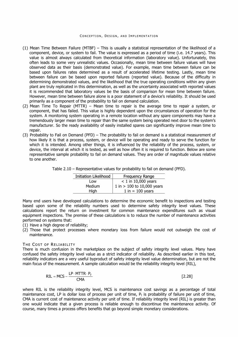
CC OO NN CC EE PP TT II OO NN ,, DD EE SS II GG NN ,, AA NN DD II MM PP LL EE MM EE NN TT AA TT II OO NN
(1) Mean Time Between Failure (MTBF) – This is usually a statistical representation of the likelihood of a component, device, or system to fail. The value is expressed as a period of time (i.e. 14.7 years). This value is almost always calculated from theoretical information (laboratory value). Unfortunately, this often leads to some very unrealistic values. Occasionally, mean time between failure values will have observed data as their basis (demonstrated value). For example, mean time between failure can be based upon failures rates determined as a result of accelerated lifetime testing. Lastly, mean time between failure can be based upon reported failures (reported value). Because of the difficulty in determining demonstrated values, and the likelihood that the true operating conditions within any given plant are truly replicated in this determination, as well as the uncertainty associated with reported values it is recommended that laboratory values be the basis of comparison for mean time between failure. However, mean time between failure alone is a poor statement of a device’s reliability. It should be used primarily as a component of the probability to fail on demand calculation.
(2) Mean Time To Repair (MTTR) – Mean time to repair is the average time to repair a system, or component, that has failed. This value is highly dependent upon the circumstances of operation for the system. A monitoring system operating in a remote location without any spare components may have a tremendously larger mean time to repair than the same system being operated next door to the system’s manufacturer. So the ready availability of easily installed spares can significantly improve mean time to repair.
(3) Probability to Fail on Demand (PFD) – The probability to fail on demand is a statistical measurement of how likely it is that a process, system, or device will be operating and ready to serve the function for which it is intended. Among other things, it is influenced by the reliability of the process, system, or device, the interval at which it is tested, as well as how often it is required to function. Below are some representative sample probability to fail on demand values. They are order of magnitude values relative to one another.
Table 2.10 – Representative values for probability to fail on demand (PFD).
IInniittiiaattiioonn LLiikkeelliihhoooodd FFrreeqquueennccyy RRaannggee Low < 1 in 10,000 years
Medium 1 in > 100 to 10,000 years High 1 in = 100 years
Many end users have developed calculations to determine the economic benefit to inspections and testing based upon some of the reliability numbers used to determine safety integrity level values. These calculations report the return on investment for common maintenance expenditures such as visual equipment inspections. The premise of these calculations is to reduce the number of maintenance activities performed on systems that: (1) Have a high degree of reliability; (2) Those that protect processes where monetary loss from failure would not outweigh the cost of
maintenance. TT HH EE CC OO SS TT OO FF RR EE LL II AA BB II LL II TT YY There is much confusion in the marketplace on the subject of safety integrity level values. Many have confused the safety integrity level value as a strict indicator of reliability. As described earlier in this text, reliability indicators are a very useful byproduct of safety integrity level value determination, but are not the main focus of the measurement. A sample calculation would be the reliability integrity level (RIL),
CMAPMTTRLP
MCSRIL f [2.28]
where RIL is the reliability integrity level, MCS is maintenance cost savings as a percentage of total maintenance cost, LP is dollar loss of process per unit of time, Pf is probability of failure per unit of time, CMA is current cost of maintenance activity per unit of time. If reliability integrity level (RIL) is greater than one would indicate that a given process is reliable enough to discontinue the maintenance activity. Of course, many times a process offers benefits that go beyond simple monetary considerations.

II NN DD UU SS TT RR II AA LL FF AA CC II LL II TT YY SS AA FF EE TT YY
RR EE FF EE RR EE NN CC EE SS AIChemE, 1993. Guidelines for Safe Automation of Chemical Processes, ISBN 0-8169-0554-1. BSI, 2002. BS EN 61508 – Functional Safety of Electrical, Electronic, Programmable Electronic Safety-Related Systems. BSI, 2003. BS IEC 61511 – Functional Safety: Safety Instrumented Systems for the Process Industry Sector. HMSO, 1991. Major Hazards Aspects of the Transport of Dangerous Substances, ISBN 0-11-885699-5. HSE Books, 2001. Reducing Risks, Protecting People, Clause 136, ISBN 0-7176-2151-0. UKOOA, 1999. Guidelines for Instrument-Based Protective Systems, Issue No. 2, Clause 4.4.3.

CC OO NN CC EE PP TT II OO NN ,, DD EE SS II GG NN ,, AA NN DD II MM PP LL EE MM EE NN TT AA TT II OO NN
CC HH AA PP TT EE RR 33
LLAAYY EERR OOFF PPRROOTTEECCTT IIOONN AANNAALLYY SS IISS ((LLOOPPAA))
II NN TT RR OO DD UU CC TT II OO NN In the 1990s, companies and industry groups devel oped standards to design, build, and maintain safety instrumented systems (SIS). A key input for the tools and techniques required to implement these standards was the required probability of failure on demand (PFD) for each safety instrumented function (SIF). Process hazard analysis (PHA) teams and project teams struggled to determine the required safety integrity level (SIL) for the safety instrumented functions (“interlocks”). The concept of layers of protection and an approach to analyze the number of layers needed was first published by the Center for Chemical Process Safety (CCPS) in the 1993 book “Guidelines for Safe Automation of Chemical Processes”. From those concepts, several companies developed internal procedures for layer of protection analysis (LOPA), and in 2001, the Center for Chemical Process Safety published a book describing layer of protection analysis. This document briefly describes the layer of protection analysis process, and discusses experience in implementing the technique. Layer of protection analysis (LOPA) is a simplifie d risk assessment tool that is uniquely useful for determining how “strong” the design should be for a safety instrumented function – “interlock” (SIF). Layer of protection analysis is a semi-quantitative tool that can estimate the required probability of failure on demand (PFD) for a safety instrumented function. It is readily applied after the process hazard analysis (PHA), for example hazard and operability analysis (HAZOP), and before fault tree analysis (FTA) or quantitative risk assessment (QRA). In most cases, the safety instrumented function’s safety integrity level requirements can be determined by layer of protection analysis without using the more time-consuming tools of fault tree analysis or quantitative risk assessment. The tool is self-documenting. The layer of protection analysis (LOPA) method is a process hazard analysis (PHA) tool. The method utilizes the hazardous events, event severity, initiating causes and initiating likelihood data developed during the hazard and operability analysis (HAZOP). The layer of protection analysis method allows the user to determine the risk associated with the various hazardous events by utilizing their severity and the likelihood of the events being initiated. Using corporate risk standards, the user can determine the total amount of risk reduction required and analyze the risk reduction that can be achieved from various layers of protection. If additional risk reduction is required after the reduction provided by process design, the basic process control system (BPCS), alarms and associated operator actions, pressure relief valves, etc., a safety instrumented function (SIF) may be required. The safety integrity level (SIL) of the safety instrumented function can be determined directly from the additional risk reduction required.
LLAA YY EE RR OO FF PPRR OO TT EE CC TT II OO NN AA NN AA LL YY SS II SS (( LLOOPPAA)) PPRR II NN CC II PP LL EE SS Layer of protection analysis (LOPA) is a semi-quantitative risk analysis technique that is applied following a qualitative hazard identification tool such as hazard and operability analysis (HAZOP). We describe layer of protection analysis as semi-quantitative because the technique does use numbers and generate a numerical risk estimate. However, the numbers are selected to conservatively estimate failure probability, usually to an order of magnitude level of accuracy, rather than to closely represent the actual performance of specific equipment and devices. The result is intended to be conservative (overestimating the risk), and is usually adequate to understand the required safety integrity level for the safety instrumented functions. If a more complete understanding of the risk is required, more rigorous quantitative techniques such as fault tree analysis or quantitative risk analysis may be required. Layer of protection analysis (LOPA) starts with an undesired consequence – usually, an event with environmental, health, safety, business, or economic impact.
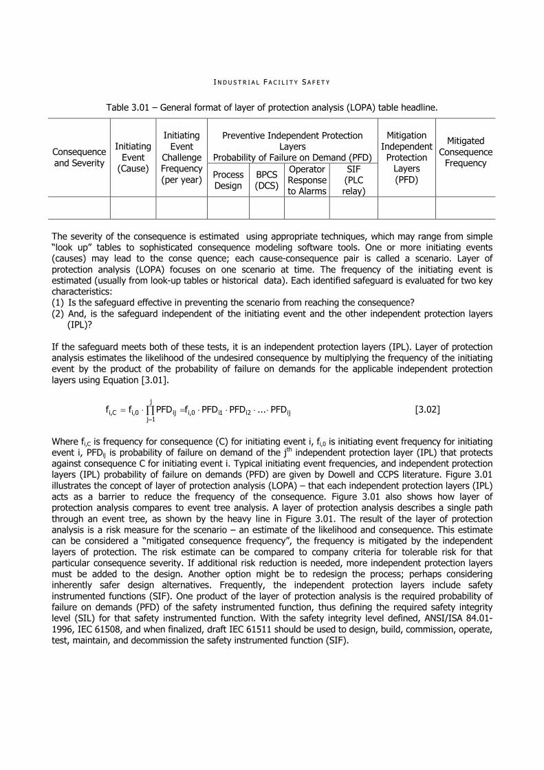
II NN DD UU SS TT RR II AA LL FF AA CC II LL II TT YY SS AA FF EE TT YY
Table 3.01 – General format of layer of protection analysis (LOPA) table headline.
Preventive Independent Protection
Layers Probability of Failure on Demand (PFD) Consequence
and Severity
Initiating Event
(Cause)
Initiating Event
Challenge Frequency (per year) Process
Design BPCS (DCS)
Operator Response to Alarms
SIF (PLC relay)
Mitigation Independent Protection
Layers (PFD)
Mitigated Consequence
Frequency
The severity of the consequence is estimated using appropriate techniques, which may range from simple “look up” tables to sophisticated consequence modeling software tools. One or more initiating events (causes) may lead to the conse quence; each cause-consequence pair is called a scenario. Layer of protection analysis (LOPA) focuses on one scenario at time. The frequency of the initiating event is estimated (usually from look-up tables or historical data). Each identified safeguard is evaluated for two key characteristics: (1) Is the safeguard effective in preventing the scenario from reaching the consequence? (2) And, is the safeguard independent of the initiating event and the other independent protection layers
(IPL)? If the safeguard meets both of these tests, it is an independent protection layers (IPL). Layer of protection analysis estimates the likelihood of the undesired consequence by multiplying the frequency of the initiating event by the product of the probability of failure on demands for the applicable independent protection layers using Equation [3.01].
ij2i1i0,i
j
1jij0,iC,i PFD...PFDPFDfPFDff
[3.02]
Where fi,C is frequency for consequence (C) for initiating event i, fi,0 is initiating event frequency for initiating event i, PFDij is probability of failure on demand of the jth independent protection layer (IPL) that protects against consequence C for initiating event i. Typical initiating event frequencies, and independent protection layers (IPL) probability of failure on demands (PFD) are given by Dowell and CCPS literature. Figure 3.01 illustrates the concept of layer of protection analysis (LOPA) – that each independent protection layers (IPL) acts as a barrier to reduce the frequency of the consequence. Figure 3.01 also shows how layer of protection analysis compares to event tree analysis. A layer of protection analysis describes a single path through an event tree, as shown by the heavy line in Figure 3.01. The result of the layer of protection analysis is a risk measure for the scenario – an estimate of the likelihood and consequence. This estimate can be considered a “mitigated consequence frequency”, the frequency is mitigated by the independent layers of protection. The risk estimate can be compared to company criteria for tolerable risk for that particular consequence severity. If additional risk reduction is needed, more independent protection layers must be added to the design. Another option might be to redesign the process; perhaps considering inherently safer design alternatives. Frequently, the independent protection layers include safety instrumented functions (SIF). One product of the layer of protection analysis is the required probability of failure on demands (PFD) of the safety instrumented function, thus defining the required safety integrity level (SIL) for that safety instrumented function. With the safety integrity level defined, ANSI/ISA 84.01-1996, IEC 61508, and when finalized, draft IEC 61511 should be used to design, build, commission, operate, test, maintain, and decommission the safety instrumented function (SIF).

CC OO NN CC EE PP TT II OO NN ,, DD EE SS II GG NN ,, AA NN DD II MM PP LL EE MM EE NN TT AA TT II OO NN
Initiating event
Success
Failure
IPL
1
Success
Failure
Success
Failure
Safe outcome
Undesired but tolerable outcome
Undesired but tolerable outcome
Consequences exceeding criteria
IPL
2
IPL
3
Cosequence occurs
Figure 3.01 – Comparison between layer of protection analysis (LOPA) and event tree analysis. The safety lifecycle defined in IEC 61511-1 requires the determination of a safety integrity level for the design of a safety-instrumented function. The layer of protection analysis (LOPA) described here is a method that can be applied to an existing plant by a multi-disciplined team to determine the required safety instrumented functions and the safety integrity level for each. The team should consist of: (1) Operator with experience operating the process under consideration. (2) Engineer with expertise in the process. (3) Manufacturing management. (4) Process control engineer. (5) Instrument and electrical maintenance person with experience in the process under consideration. (6) Risk analysis specialist. At least one person on the team should be trained in the layer of protection analysis (LOPA) methodology. The information required for the layer of protection analysis is contained in the data collected and developed in the hazard and operability analysis (HAZOP). Table 3.01 shows a typical spreadsheet that can be used for the layer of protection analysis. Impact Event Each impact event (consequence) determined from the hazard and operability analysis is entered in the spreadsheet. Severity Level Severity levels of Minor (M), Serious (S), or Extensive (E) are next selected for the impact event. Likelihood values are events per year, other numerical values are average probabilities of failure on demand (PFDavg). Initiating Event (Cause) All of the initiating causes of the impact event are listed. Impact events may have many initiating causes, and it is important to list all of them. Initiation Likelihood Likelihood values of the initiating causes occurring, in events per year, are entered. The experience of the team is very important in determining the initiating cause likelihood.

II NN DD UU SS TT RR II AA LL FF AA CC II LL II TT YY SS AA FF EE TT YY
Protection Layers Each protection layer consists of a grouping of equipment and administrative controls that function in concert with the other layers. Protection layers that perform their function with a high degree of reliability may qualify as independent protection layer (IPL). The criteria to qualify a protection layer (PL) as an independent protection layers are: (1) The protection provided reduces the identified risk by a large amount, that is, a minimum of a ten-fold
reduction. (2) The protective function is provided with a high degree of availability (90% or greater). It has the following important characteristics: (1) Specificity – An independent protection layer (IPL) is designed solely to prevent or to mitigate the
consequences of one potentially hazardous event (e.g. a runaway reaction, release of toxic material, a loss of containment, or a fire). Multiple causes may lead to the same hazardous event; and, therefore, multiple event scenarios may initiate action of one independent protection layer.
(2) Independence – An independent protection layer (IPL) is independent of the other protection layers associated with the identified danger.
(3) Dependability – It can be counted on to do what it was designed to do. Both random and systematic failures modes are addressed in the design.
(4) Auditability – It is designed to facilitate regular validation of the protective functions. Proof testing and maintenance of the safety system is necessary.
Only those protection layers that meet the tests of availability, specificity, independence, dependability, and auditability are classified as independent protection layers. If a control loop in the basic process control system (BPCS) prevents the impacted event from occurring when the initiating cause occurs, credit based on its average probabilities of failure on demand (PFDavg) is claimed. Additional Mitigation Mitigation layers are normally mechanical, structural, or procedural. Examples would be: (1) Pressure relief devices; (2) Dikes; (3) Restricted access. Mitigation layers may reduce the severity of the impact event but not prevent it from occurring. Examples would be: (1) Deluge systems for fire or fume release; (2) Fume alarms; (3) Evacuation procedures. Independent Protection Layers Protection layers that meet the criteria for independent protection layer (IPL). Intermediate Event Likelihood The intermediate event likelihood is calculated by multiplying the initiating likelihood by the probability of failure on demands (PFD) of the protection layers and mitigating layers. The calculated number is in units of events per year. If the intermediate event likelihood is less than your corporate criteria for events of this severity level, additional protection layers (PL) are not required. Further risk reduction should, however, be applied if economically appropriate. If the Intermediate event likelihood is greater than your corporate criteria for events of this severity level, additional mitigation is required. Inherently safer methods and solutions should be considered before additional protection layers in the form of safety instrumented systems (SIS) are applied. If the above attempts to reduce the intermediate likelihood below corporate risk criteria fail, a safety instrumented systems (SIS) is required. Safety Instrumented Functions (SIF) Integrity Level If a new safety instrumented function (SIF) is needed, the required integrity level can be calculated by dividing the corporate criteria for this severity level of event by the intermediate event likelihood. A

CC OO NN CC EE PP TT II OO NN ,, DD EE SS II GG NN ,, AA NN DD II MM PP LL EE MM EE NN TT AA TT II OO NN
probabilities of failure on demand (PFDavg) for the safety instrumented function below this number is selected as a maximum for the safety instrumented systems (SIS). Mitigated Event Likelihood The mitigated event likelihood is now calculated by multiplying intermediate event likelihood (IEL) and safety instrumented function (SIF) integrity level. This is continued until the team has calculated a mitigated event likelihood for each impact event that can be identified. Total Risk The last step is to add up all the mitigated event likelihood for serious and extensive impact events that present the same hazard. For example, the mitigated event likelihood for all serious and extensive events that cause fire would be added and used in formulas like the following,
Risk of Fatality due to Fire = [Mitigated Event Likelihood of all flammable material release][Probability of Ignition][Probability of a person in the area][Probability of Fatal Injury in the Fire]
Serious and extensive impact events that would cause a toxic release could use the following formula,
Risk of Fatality due to Toxic Release = [Mitigated Event Likelihood of all Toxic Releases][Probability of a person in the area][Probability of Fatal Injury in the Release]
The expertise of the risk analyst specialist and the knowledge of the team are important in adjusting the factors in the formulas to conditions and work practices of the plant and affected community. The total risk to the corporation from this process can now be determined by totalling the results obtained from applying the formulas. If this meets or is less than the corporate criteria for the population affected, the layer of protection analysis (LOPA) is complete. However, since the affected population may be subject to risks from other existing units or new projects, it is wise to provide additional mitigation if it can be accomplished economically.
II MM PP LL EE MM EE NN TT II NN GG LLAA YY EE RR OO FF PPRR OO TT EE CC TT II OO NN AA NN AA LL YY SS II SS (( LLOOPPAA)) Some important considerations and experience in implementing layer of protection analysis (LOPA) are discussed by Dowell, and these are summarized briefly below. A greatly expanded discussion of these points can be found in the original reference. The important considerations are as follows: (1) Team Makeup – Some organizations conduct layer of protection analysis as a part of the process hazard
analysis (PHA) review, using the process hazard analysis team. This can be efficien t because the team is familiar with the scenario and decisions can be recorded as part of the process hazard analysis recommendations. This approach works best when the risk tolerance criteria are applied to each scenario individually. Other companies have found it to be more efficient to capture the list of potential layer of protection analysis scenarios during the process hazard analysis, for later evaluation by a smaller team (perhaps just a process engineer and a person skilled in layer of protection analysis). The layer of protection analysis team may then report back to the process hazard analysis team on the re sults of their evaluation. Either approach may be used successfully. The important factor is that the process knowledge is incorporated in the layer of protection analysis and that the layer of protection analysis methodology is applied correctly and consistently.
(2) One Cause, One Consequence, One Scenario. It is critical that each layer of protection analysis scenario have only one cause and one consequence. Users may be tempted to combine causes that lead to the same consequence to save time in the analysis and documentation. Unfortunately, each independent protection layers (IPL) may not protect against each initiating event. For example, a safety instrumented function (SIF) that blocks the feed flow into a reactor protects against high pressure from the feed streams, but this safety instrumented function does not protect against high pressure caused by internal reaction. It is important each candidate independent protection layers (IPL) be evaluated for its effectiveness against a single initiating event leading to a single consequence.

II NN DD UU SS TT RR II AA LL FF AA CC II LL II TT YY SS AA FF EE TT YY
(3) Understanding what constitutes an independent protection layer (IPL). An independent protection layers
is a device, system, or action that is capable of preventing a scenario from proceeding to its undesired consequence independent of the initiating event or the action of any other layer of protection associated with the scenario. The effectiveness and independence of an independent protection layer must be auditable. All independent protection layers are safeguards, but not all safeguards are independent protection layers. Each safeguard identified for a scenario must be tested for conformance with this definition. The following keywords may be helpful in evaluating an independent protection layer (IPL). The “three Ds” help determine if a candidate is an independent protection layer (IPL): Detect – Most independent protection layers detect or sense a condition in the scenario; Decide – Many independent protection layers make a decision to take action or not; Deflect – All independent protection layers deflect the undesired consequence by preventing it. The “four Enoughs” help evaluate the effectiveness of a candidate independent protection layer (IPL): “Big Enough?”, “Fast Enough?”, “Strong Enough?”, “Smart Enough?”. The “Big I” – Remember that the independent protection layer (IPL) must be independent of the initiating event and all other independent protection layers.
(4) Understanding Independence. A critical issue for layer of protection analysis (LOPA) is determining whether independent protection layers (IPL) are independent from the initiating event and from each other. The layer of protection analysis (LOPA) methodology is based on the assumption of independence. If there are common mode failures among the initiating event and independent protection layers, the layer of protection analysis will underestimate the risk for the scenario. Dowell and CCPS discuss how to ensure independence, and provide several useful examples.
(5) Procedures and Inspections. Procedures and inspections cannot be counted as independent protection layers (IPL). They do not have the ability to detect the initiating event, cannot make a decision to take action, and cannot take action to preven t the consequence. Inspections and tests of the independent protection layer do not count as another independent protection layer. They do affect the probability of failure on demands (PFD) of the independent protection layer (IPL).
(6) Mitigating independent protection layers (IPL). An independent protection layer may prevent the consequence identified in the scenario, but, through its proper functioning, it may generate another less severe, but still undesirable, consequence. A rupture disk on a vessel is an example. It prevents overpressurization of the vessel (although not 100% of the time, the rupture disk does have a probability of failure on demands). However, the proper operation of the rupture disk results in a loss of containment from the vessel to the environment or a containment or treatment system. This best way do deal with this situation is to create another layer of protection analysis (LOPA) scenario to estimate the frequency of the release through the rupture disk, its consequence, and then determine if it meets the risk tolerance criteria.
(7) Beyond layer of protection analysis (LOPA). Some scenarios or groups of scenarios are too complex for layer of protection analysis. A more detailed risk assessment tool such as event tree analysis, fault tree analysis, or quantitative risk analysis is needed. Some examples where this might be true include: A system that has shared components be tween the initiating event and candidate independent protection layers (IPL), and no cost effective way of providing independence. This system violates the layer of protection analysis requirement for independence between initiating event and independent protection layers (IPL). A large complex system with many layer of protection analysis scenarios, or a variety of different consequences impacting different populations. This system may be more effectively analyzed and understood using quantitative risk analysis.
(8) Risk Criteria. Implementation of layer of protection analysis (LOPA) is easier if an organization has defined risk tolerance criteria. It is ve ry difficult to make risk ba sed decisions without these criteria, which are used to decide if the frequency of the mitigated consequence (with the independent protection layers in place) is low enough. CCPS provides guidance and references on how to develop and use risk criteria.
(9) Consistency. When an organization implements layer of protection analysis (LOPA), it is important to establish tools, including aids like look-up tables for consequence severity, initiating event frequency, and probability of failure on demands (PFD) for standard independent protection layers (IPL). The calculation tools must be documented, and users trained. All layer of protection analysis (LOPA) practitioners in an organization must use the same rules in the same way to ensure consistent results.

CC OO NN CC EE PP TT II OO NN ,, DD EE SS II GG NN ,, AA NN DD II MM PP LL EE MM EE NN TT AA TT II OO NN
Process safety engineers and safety integrity level (SIL) assignment teams from many companies have concluded that layer of protection analysis (LOPA) is an effective tool for safety integrity level assignment. Layer of protection analysis requires fewer resources and is faster than fault tree analysis or quantitative risk assessment. If more detailed analysis is needed, the layer of protection analysis scenarios and candidate IPLs provide an excellent starting point. Layer of protection analysis (LOPA) has the following advantages: (1) Focuses on severe consequences; (2) Considers all the identified initiating causes; (3) Encourages system perspective; (4) Confirms which IPLs are effective for which initiating causes; (5) Allocates risk reduction resources efficiently; (6) Provides clarity in the reasoning process; (7) Documents everything that was considered; (8) Improves consistency of SIL assignment; (9) Offers a rational basis for managing IPLs in an operating plant. LL AA YY EE RR OO FF PP RR OO TT EE CC TT II OO NN AA NN AA LL YY SS II SS (( LL OO PP AA )) EE XX AA MM PP LL EE FF OO RR II MM PP AA CC TT EE VV EE NN TT II Following is an example of the layer of protection analysis (LOPA) methodology that addresses one impact event identified in the hazard and operability analysis (HAZOP). Impact Event and Severity Level The hazard and operability analysis (HAZOP) identified high pressure in a batch polymerisation reactor as a deviation. The stainless steel reactor is connected in series to a packed steel fiber reinforced plastic column and a stainless steel condenser. Rupture of the fiber reinforced plastic column would release flammable vapor that would present the possibility for fire if an ignition source is present. Using Table 3.02 severity level serious is selected by the layer of protection analysis (LOPA) team since the impact event could cause a serious injury or fatality on site.
Table 3.02 – Impact event severity levels.
IImmppaacctt EEvveenntt LLeevveell CCoonnsseeqquueennccee
Minor (M) Impact initially limited to local area of event with potential for Broader consequence, if corrective action not taken.
Serious (S) Impact event could cause any serious injury or fatality on site or off site. Extensive (E) Impact event that is five or more times severe than a serious event.
Initiating Causes The hazard and operability analysis (HAZOP) listed two initiating causes for high pressure: Loss of cooling water to the condenser and failure of the reactor steam control loop. Initiating Likelihood Plant operations have experienced loss in cooling water once in 15 years in this area. The team selects once every 10 years as a conservative estimate of cooling water loss. It is wise to carry this initiating cause all the way through to conclusion before addressing the other initiating cause (failure of the reactor steam control loop in this case). Protection Layers Design The process area was designed with an explosion proof electrical classification and the area has a process safety management plan in effect. One element of the plan is a management of change procedure for replacement of electrical equipment in the area. The layer of protection analysis (LOPA) team estimates that the risk of an ignition source being present is reduced by a factor of 10 due to the management of change procedures. Basic Process Control System (BPCS) High pressure in the reactor is accompanied by high temperature in the reactor. The basic process control system (BPCS) has a control loop that adjusts steam input to the reactor jacket based on temperature in the

II NN DD UU SS TT RR II AA LL FF AA CC II LL II TT YY SS AA FF EE TT YY
reactor. The basic process control system would shut off steam to the reactor jacket if the reactor temperature is above setpoint. Since shutting off steam is sufficient to prevent high pressure, the basic process control system is a protection layer. The basic process control system (BPCS) is a very reliable distributed control system (DCS) and the production personnel have never experienced a failure that would disable the temperature control loop. The layer of protection analysis (LOPA) team decides that a average probability of failure on demands (PFDavg) of 0.1 is appropriate and enters 0.1 under basic process control system (0.1 is the minimum allowable for the basic process control system). Alarms There is a transmitter on cooling water flow to the condenser, and it is wired to a different basic process control system (BPCS) controller than the temperature control loop. Low cooling water flow to the condenser is alarmed and utilizes operator intervention to shut off the steam. The alarm can be counted as a protection layer since it is located in a different basic process control system controller than the temperature control loop. The layer of protection analysis (LOPA) team agrees that a 0.1 average probability of failure on demands (PFDavg) is appropriate since an operator is always present in the control room and enters 0.1 under alarms column. Additional Mitigation Access to the operating area is restricted during process operation. Maintenance is only performed during periods of equipment shut down and lock out. The process safety management plan requires all non-operating personnel to sign into the area and notify the process operator. Because of the enforced restricted access procedures, the layer of protection analysis (LOPA) teams estimate that the risk of personnel in the area is reduced by a factor of 10. Therefore 0.1 is entered under additional mitigation column. Independent Protection Layer (IPL) The reactor is equipped with a relief valve that has been properly sized to handle the volume of gas that would be generated during over temperature and pressure caused by cooling water loss. Since the relief valve is set below the design pressure of the fiber glass column and there is no possible human failure that could isolate the column from the relief valve during periods of operation, the relief valve is considered a protection layer. The relief valve is removed and tested once a year and never in 15 years of operation has any pluggage been observed in the relief valve or connecting piping. Since the relief valve meets the criteria for an independent protection layer (IPL), it is listed in and assigned a average probability of failure on demands (PFDavg) of 0.01. Intermediate Event Likelihood The columns are now multiplied together and the product is entered under intermediate event likelihood column. Safety Instrumented Systems (SIS) The mitigation obtained by the protection layers are sufficient to meet corporate criteria, but additional mitigation can be obtained for a minimum cost since a pressure transmitter exists on the vessel and is alarmed in the basic process control system (BPCS). The layer of protection analysis (LOPA) team decides to add a safety instrumented function (SIF) that consists of a current switch and a relay to de-energize a solenoid valve connected to a block valve in the reactor jacket steam supply line. The safety instrumented function is designed to the lower range of SIL 1 rating, with a average probability of failure on demands (PFDavg) of 0.01, entered under safety instrumented function (SIF) integrity level. The mitigated event likelihood is now calculated by multiplying intermediate event likelihood column by safety instrumented function (SIF) integrity level column and putting the result (1109) in mitigated event likelihood column. Next Event The layer of protection analysis (LOPA) team now considers the second initiation event (failure of reactor steam control loop). Table 3.03 is used to determine the likelihood of control valve failure and 0.1 is entered under initiation likelihood column. The protection layers obtained from process design, alarms, additional mitigation and the safety instrumented systems (SIS) still exist if a failure of the steam control loop occurs.

CC OO NN CC EE PP TT II OO NN ,, DD EE SS II GG NN ,, AA NN DD II MM PP LL EE MM EE NN TT AA TT II OO NN
The only protection layer lost is the basic process control system (BPCS). The layer of protection analysis team calculates the intermediate likelihood (1105) and the mitigated event likelihood (1.1108).
Table 3.03 – Typical protection layer (prevention & mitigation) probability of failure on demands (PFD).
IInnddeeppeennddeenntt PPrrootteeccttiioonn LLaayyeerr ((IIPPLL)) PPrroobbaabbiilliittyy ooff FFaaiilluurree oonn DDeemmaanndd ((PPFFDD)) Control loop 1.0101 Relief valve 1.0102 Human performance (trained, no stress) 1.0102 Human performance (under stress) 0.5 to 1.0 Operator Response to Alarms 1.0101 Vessel pressure rating above maximum challenge from internal and external pressure sources 1.0104 or better
Table 3.04 – Initiation likelihood.
CCaatteeggoorryy DDeessccrriippttiioonn LLiikkeelliihhoooodd ((ppeerr yyeeaarr))
Low
A failure or series of failures with a very low probability of occurrence within the expected lifetime of the plant. Examples: Three or more simultaneous; Instrument, valve, or human failures; Spontaneous failure of single tanks or process vessels.
f < 1.0104
Medium
A failure or series of failures with a low probability of occurrence within the expected lifetime of the plant. Examples: Dual instrument or valve failures; Combination of instrument failures and operator errors; Single failures of small process lines or fittings.
1.0104< f < 1.0102
High A failure can reasonably be expected to occur within the expected lifetime of the plant. Examples: Process Leaks; Single instrument or valve failures; Human errors that could result in material releases.
1.0102 < f
The layer of protection analysis team would continue this analysis until all the deviations identified in the hazard and operability analysis (HAZOP) have been addressed. The last step would be to add the mitigated event likelihood for the serious and extensive events that present the same hazard. In this example, if only the one impact event was identified for the total process, the number would be 1108. Since the probability of ignition was accounted for under process design (0.1) and the probability of a person in the area was accounted for under additional mitigation (0.1), the equation for risk of fatality due to fire reduces to, Risk of Fatality Due to Fire = [Mitigated Event Likelihood of all flammable material releases][Probability of
Fatal Injury in the fire] or
Risk of Fatality Due to Fire = 1.1108 0.5 = 5.5109 This number is below the corporate criteria for this hazard so the work of the layer of protection analysis (LOPA) team is complete. LL AA YY EE RR OO FF PP RR OO TT EE CC TT II OO NN AA NN AA LL YY SS II SS (( LL OO PP AA )) EE XX AA MM PP LL EE FF OO RR II MM PP AA CC TT EE VV EE NN TT II II The hazard and operability analysis (HAZOP) identified high pressure as a deviation. One consequence of high pressure in the column was catastrophic rupture of the column, if it exceeded its design pressure. In the layer of protection analysis (LOPA), this impact event is listed as extensive for severity class, since there is potential for five or more fatalities. The maximum target likelihood for extensive impact events is 1.0108 per year. The hazard and operability analysis (HAZOP) listed several initiating causes for this impact event. One initiating cause was loss of cooling tower water to the main condenser. The operators said this happened about once every ten years. Challenge likelihood is 0.1 per year. The layer of protection analysis

II NN DD UU SS TT RR II AA LL FF AA CC II LL II TT YY SS AA FF EE TT YY
(LOPA) team identified one process design independent protection layer (IPL) for this impact event and this cause. The maximum allowable working pressure of the distillation column and connected equipment is greater than the maximum pressure that can be generated by the steam reboiler during a cooling tower water failure. Its probability of failure on demand (PFD) is 1.0102. The basic process control system (BPCS) for this plant is a distributed control system (DCS). The distributed control system contains logic that trips the steam flow valve and a steam RCV on high pressure or high temperature of the distillation column. This logic's primary purpose is to place the control system in the shut-down condition after a trip so that the system can be restarted in a controlled manner; it can prevent the impact event. However, no probability of failure on demand (PFD) credit is given for this logic since the valves it uses are the same valves used by the safety instrumented system (SIS) – the distributed control system (DCS) logic does not meet the test of independence for an independent protection layer. High pressure and temperature alarms displayed on the distributed control system can alert the operator to shut off the steam to the distillation column, using a manual valve if necessary. This protection layer meets the criteria for an independent protection layer, the sensors for these alarms are separate from the sensors used by the safety instrumented systems. The operators should be trained and drilled in the response to these alarms. Safety instrumented systems logic implemented in a PLC will trip the steam flow valve and a steam RCV on high distillation column pressure or high temperature using dual sensors separate from the distributed control system. The PLC has sufficient redundancy and diagnostics such that the safety instrumented systems has a probability of failure on demands of 1.0103 or SIL 3 rating. The distillation column has additional mitigation of a pressure relief valve designed to maintain the distillation column pressure below the maximum allowable working pressure when cooling tower water is lost to the condenser. Its probability of failure on demand is 1.0102. The number of independent protection layers is three. The mitigated event likelihood for this cause-consequence pair is calculated by multiplying the challenge likelihood by the independent protection layer probability of failure on demands,
CChhaalllleennggee PPrroocceessss AAllaarrmmss aanndd SSIISS RReelliieeff MMiittiiggaatteedd EEvveenntt LLiikkeelliihhoooodd DDeessiiggnn PPrroocceedduurreess VVaallvvee LLiikkeelliihhoooodd
1.0101 1.0102 1.0101 1.0103 1.0102 = 1.0109
The value of 1.0109 is less than the maximum target likelihood of 1.0108 for extensive impact events. Note that the relief valve protects against catastrophic rupture of the distillation column, but it introduces another impact event, a toxic release.
II NN TT EE GG RR AA TT II NN GG HHAA ZZ AA RR DD AA NN DD OO PP EE RR AA BB II LL II TT YY AA NN AA LL YY SS II SS ((HHAAZZOOPP)) ,, SSAA FF EE TT YY
II NN TT EE GG RR II TT YY LL EE VV EE LL ((SSII LL )) ,, AA NN DD LLAA YY EE RR OO FF PPRR OO TT EE CC TT II OO NN AA NN AA LL YY SS II SS (( LLOOPPAA)) Traditionally, a hazard and operability (HAZOP) study and safety integrity level (SIL) assessment determination (usually using the risk graph or layer of protection analysis methodology) are two separate facilitated sessions, which produce two unique databases. Safety integrity level validation is yet a third requirement of the International Electro technical Commission (IEC) 61511 standards that demands the use of another set of tools and produces a third database. Trying to manage the recommendations of these interconnected studies is extremely difficult. In the integrated approach, only one facilitated session is required for hazard and operability study and safety integrity level assessment. Only one database is created, and it is used to perform safety integrity level validation. In addition to being a secure and auditable database, this single database is also part of a complete “handover package” that operators need to ensure and maintain the safety integrity level integrity assigned to each safety integrity level loop. Some demonstrated benefits of the integrated approach are a minimum 30% time and costs savings; a single auditable database; elimination of mathematical errors during safety integrity level validation; creation of a complete electronic handover data package and the capability of operators to easily model proposed changes to their maintenance and testing plans (safety integrity level optimization) using the same database.

CC OO NN CC EE PP TT II OO NN ,, DD EE SS II GG NN ,, AA NN DD II MM PP LL EE MM EE NN TT AA TT II OO NN
Deviation
Cause
Consequence
Safeguard
Recommendation
Cause Frequency
Risk Matrix
Consequence Severity
Hazard and Operability Analysis(HAZOP) Information
Layer of Protection Analysis(LOPA) InformationImpact Event
Initiating Cause
Cause Likelihood
Process Design(IPL & PFD)
BPCS(IPL & PFD)
Alarms, Procedures(IPL & PFD)
SIS(IPL & PFD)
Additional Mitigation(IPL & PFD)
Mitigated EventLikelihood
Event Severity
Target Mitigated EventLikelihood
Mitigated Likelihoodless than target?
Add IPLs or redesignthe process NO
Continue with nextConsequence-Cause pair
YES
Totalize MitigatedEvent Likelihoods for
whole process
Figure 3.02 – Relationship between hazard and operability (HAZOP) and layer of protection analysis (LOPA). MM EE TT HH OO DD OO LL OO GG YY The integrated hazard and operability (HAZOP) and safety integrity level (SIL) study is initiated by calling a meeting (or session) usually comprising of the operating company, the engineering consultancy company (if this is a new project) and the hazard and operability and safety integrity level facilitator with his scribe (who is usually an independent third party). The team of engineers should definitely consist of chemical (or process engineers), instrumentation and safety engineers. Other engineers are optional depending on their need during the course of the session. The session has the following steps in the order as listed below.

II NN DD UU SS TT RR II AA LL FF AA CC II LL II TT YY SS AA FF EE TT YY
Hazard And Operability (HAZOP) Study A hazard and operability (HAZOP) study is used to identify major process hazards or operability issues related to the process design. Major process hazards include the release of hazardous materials and energy. The focus of the study is to address incidents, which may impact on public health and safety, worker safety in the workplace, economic loss, the environment, and the company’s reputation. The inputs to the hazard and operability (HAZOP) are the Process and Instrumentation Diagrams (P&ID), Cause and Effect charts (C&E) and the operating company’s risk matrix which is a matrix quantifying the risk level depending on the likelihood and severity. A typical risk matrix would look as given below in Table 3.05.
Table 3.05 – A typial risk matrix used in hazard and operability (HAZOP) study.
FFrreeqquueenntt ((mmoorree tthhaann oonnccee ppeerr yyeeaarr))
PPrroobbaabbllee ((oonnccee eevveerryy ffoouurr yyeeaarrss))
OOccccaassiioonnaall ((oonnccee eevveerryy 2255 yyeeaarrss))
RReemmoottee ((nnoott iinn tthhee lliiffee ooff tthhee ffaacciilliittyy))
SSeevveerriittyy LLeevveell 11 ((CCrriittiiccaall))
Priority 1 (Unacceptable)
Priority 1 (Unacceptable)
Priority 1 (Unacceptable)
Priority 2 (High)
SSeevveerriittyy LLeevveell 22 ((HHiigghh))
Priority 1 (Unacceptable)
Priority 2 (High)
Priority 2 (High)
Priority 3 (Medium)
SSeevveerriittyy LLeevveell 33 ((MMooddeerraattee))
Priority 2 (High)
Priority 3 (Medium)
Priority 4 (Low)
Priority 4 (Low)
SSeevveerriittyy LLeevveell 44 ((MMiinnoorr))
Priority 3 (Medium)
Priority 4 (Low)
Priority 4 (Low)
Priority 4 (Low)
The outputs from the hazard and operability (HAZOP) are the risk ranking of each identified cause of process deviation and recommendations to lower the risk involved. These recommendations are given in the form of safeguards. SS AA FF EE TT YY II NN TT EE GG RR II TT YY LL EE VV EE LL (( SS II LL )) AA NN DD LL AA YY EE RR OO FF PP RR OO TT EE CC TT II OO NN AA NN AA LL YY SS II SS (( LL OO PP AA )) AA SS SS EE SS SS MM EE NN TT Safety integrity level (SIL) and layer of protection analysis (LOPA) assessment study is to assess the adequacy of the safety protection layers (SPL) or safeguards that are in place to mitigate against hazardous events relating to major process hazards, identify those safety protection layers or safeguards that do not meet the required risk reduction for a particular hazard, and make reasonable recommendations where a hazard generates a residual risk that needs further risk reduction. This is done by defining the tolerable frequency (TF). The tolerable frequency of the process deviation is a number which is derived from the level of the risk identified from the hazard and operability (HAZOP) risk matrix. It indicates the period of occurrence, in terms of years, of the process deviation which the operating company can tolerate. For example a tolerable frequency of 104 indicates that the company can tolerate the occurrence of the process deviation once in 10,000 years. The mitigation frequency (MF) is derived as a calculation from the likelihood of each cause and the probability of failure on demand (PFD) of the safety protection layers (SPL). The inputs to the safety integrity level (SIL) and layer of protection analysis (LOPA) assessment are the process deviations, causes, risk levels and safeguards identified during the hazard and operability (HAZOP). The safety integrity level (SIL) and layer of protection analysis (LOPA) assessment recommend the safety protection layers (SPL) to be designed to meet the process hazard. Recommendations In the event that the mitigation frequency (MF) is not less than the tolerable frequency (TF), more safety protection layers (SPL) are recommended, their probability of failure on demand (PFD) values are assumed and it is included in the equation of the mitigation frequency to get it less than the tolerable frequency. These safety protection layers are recommended as safeguards to decrease the risk of the consequences because of the deviation (or cause) being analyzed. The session ends with the mitigation frequency values of all the layer of protection analysis scenarios derived lees than the tolerable frequency. Safety Integrity Level (SIL) and Layer of Protection Analysis (LOPA) Assessment Validation This is done after the session by the reliability or safety engineer. The methodology is to calculate the probability of failure on demand (PFD) values of the identified safety protection layers (SPL), then derive the mitigation frequency (MF) as a calculation from the likelihood of each cause and the probability of failure on demand of the safety protection layers. If the total mitigation frequency (MF) of all the causes is less than

CC OO NN CC EE PP TT II OO NN ,, DD EE SS II GG NN ,, AA NN DD II MM PP LL EE MM EE NN TT AA TT II OO NN
the tolerable frequency (TF), which is defined as a numerical value from the hazard and operability (HAZOP) risk matrix, the integrated study is complete. This validates the assumed probability of failure on demand values of the safety protection layers during the session. TT HH EE II NN TT EE GG RR AA TT EE DD HH AA ZZ AA RR DD AA NN DD OO PP EE RR AA BB II LL II TT YY (( HH AA ZZ OO PP )) AA NN DD SS AA FF EE TT YY II NN TT EE GG RR II TT YY LL EE VV EE LL (( SS II LL )) PP RR OO CC EE SS SS The following process is used in a session for each of the identified nodes during an hazard and operability (HAZOP) study: (1) The process engineer describes the intention of the node. (2) Concerns and hazards within the node are recorded under the discussed node notes. (3) The team applies process parameter deviations to each node and identifies the associated hazards. (4) Causes and initiating events to those hazards are identified, and recorded. (5) The resulting consequences are identified, categorized, and recorded based on the consequence
grading in the operating company’s risk matrix. (6) The likelihood of the initiating event is then assigned by the group and recorded based on the risk
matrix. (7) The resulting risk score based on the consequence and likelihood scores are recorded not taking credit
for any of the safeguards in place, as per the risk matrix (8) An identification of the safeguards and an evaluation as safety protection layers (SPL) is then carried
out. (9) The risk is re-scored taking into account the identified safeguards which are independent safety
protection layers (SPL). Usually a standard safety integrity level (SIL) value is assigned to the safety protection layers (SPL) which are validated outside the session for accuracy.
(10) If sufficient independent layers of protection are identified to reduce the risk to the tolerable level (TF), then no further safeguards are identified and no recommendations are required.
(11) If the risk with safeguards are high and not meeting the tolerable frequency, then recommendations and actions are developed in the aim of reducing the risk below the tolerable frequency (TF).
(12) The implementation of those actions and recommendations are assigned to the responsible party and individual. The recommended safety protection layers are validated and their probability of failure on demand (PFD) numbers are used to calculate if the mitigation frequency (MF) is less than the tolerable frequency (TF).
(13) The process is repeated covering the applicable parameters, deviations, and nodes. In the following example, a hazard and operability (HAZOP) related with “High Level” in a storage tank is considered. As per the hazard and operability (HAZOP) process, all the causes have been identified, consequences listed and risk ranking done without and with the existing safeguards (SPLs). From the hazard and operability (HAZOP), the causes of deviation are listed as layer of protection analysis (LOPA) causes, their likelihoods identified and the safeguards are listed as protection layers (SPL). The probability of failure on demand (PFD) value of each safety protection layer (SPL) is either manually entered or linked to a calculated value. If the mitigation frequency (MF) is less than tolerable frequency (as in the case of this example), it implies that some additional safety protection layers (SPL) are required to meet the tolerable frequency (TF). CC OO NN CC LL UU SS II OO NN By integrating hazard and operability (HAZOP) and safety integrity level (SIL) process into one session, the time and cost to conduct these sessions are reduced, there is more data integrity as the same team conducts both the studies and it removes the subjectivity which comes out of a pure hazard and operability session. An integrated study is a semi-quantitative technique and applies much more rigor than a hazard and operability study alone. It determines if the existing safeguards are enough and if proposed safeguards are warranted. It tightly couples the risk tools (matrices, risk graphs) of a corporation.

II NN DD UU SS TT RR II AA LL FF AA CC II LL II TT YY SS AA FF EE TT YY
MM OO DD II FF YY II NN GG LLAA YY EE RR OO FF PPRR OO TT EE CC TT II OO NN AA NN AA LL YY SS II SS (( LLOOPPAA)) FF OO RR II MM PP RR OO VV EE DD
PP EE RR FF OO RR MM AA NN CC EE Layers of protection analysis (LOPA) is a semi-quantitative risk analysis method that has been popularized by the American Institute of Chemical Engineers (AIChE) book “Layers of Protection Analysis – Simplified Process Risk Assessment” (2001). Finding wide support in the chemical, refining, and pipeline industries, the layer of protection analysis (LOPA) process has become a popular tool for assessing risk. The layer of protection analysis (LOPA) process is built upon the principle that process experts in a given industry are cognizant of and accurate in assessing the severity of possible process events, but do a poor job of assessing the likelihood of these possible process events. Because risk is composed both of severity and likelihood, a divergence in either of the factors gives a skewed assessment of true risk. Layer of protection analysis (LOPA) attempts to overcome the inherent “human-nature problem” of misdiagnosing likelihood by taking likelihoods from insurance industry data. Using historical data, the likelihood is more likely to be accurate. Layer of protection analysis suffers from a number of shortcomings. Among these is the fact that each layer of protection analysis is restricted to a single cause-consequence pair. When multiple causes can instigate the same consequence, multiple layer of protection analyses must sometimes be done. When a single cause can instigate multiple consequences, multiple layer of protection analyses must sometimes be done. An additional shortcoming is that layer of protection analysis (LOPA) is a coarse tool. Layer of protection analysis (LOPA) likelihoods are broken down into orders of magnitude change, and exact probabilities are impossible to calculate unless a large amount of field data is available. The independent protection layers (IPL) that protect against a specific scenario are also given probabilities-of-failure-on-demand (PFD) that are broken down into orders of magnitude change. Because layer of protection analysis (LOPA) has been so widely adopted over the past five years, and because its penetration of the process industries has been so deep, a broad and deep knowledge base has been developed. The first consequence of such wide acceptance has been an expansion of layer of protection analysis’ scope. The original layer of protection analysis (LOPA) book provided example tables that gave industry and insurance probabilities of a variety of process events. This table lists such items as “loss of cooling” and “human error” without offering much guidance on their application. CC HH AA NN GG EE SS TT OO TT HH EE II NN II TT II AA TT II NN GG EE VV EE NN TT SS Many companies were frustrated by the limitations of the initiating event frequency tables and proceeded to expand the number of items in the table. The addition of new causes made the layer of protection analysis (LOPA) process more flexible and able to cover more of the scenarios developed in a typical process hazards analysis (PHA). A typical table in use for 2006 is shown below (see Table 3.06). Note that a wider variety of causes has been included in Table 3.06 than was originally provided in the layer of protection analysis (LOPA) textbook. Layer of protection analysis (LOPA) practitioners are also allowed to modify the table values, based on field failure experience or on the number of opportunities for the initiating event to occur. In every case where a modification of the table value is made, the layer of protection analysis report for that incident should include a clear and defensible rationale for why the table value was modified. It is best to provide a specific procedure for deviation from the initiating events table values, so that consistency can be achieved over time and over the multiple sites of a company. Each company should strive to provide an internal guidance document so that all sites will be consistent in their application of layer of protection analysis (LOPA) initiating event frequencies. In cases where inconsistency is found in a review of layer of protection analyses, some companies ban the modification of the layer of protection analysis (LOPA) values for initiating events. Consistency is generally preferable unless there is a strong rationale for exception. Also, in order to maintain consistency, most companies have a procedure for adding new causes to the initiating events table. These new causes and their likelihoods should receive formal review and acceptance before being used. A formal, periodic review should be made to verify that the initiating events table is consistent with not only local field experience but also with wider industry practice. Such verification can be done through internal incident reviews, through industry associations, through employment of outside consultants with experience specific to the layer of protection analysis (LOPA) procedures of your industry, or through commercial and insurance databases that are typically available for a fee.

CC OO NN CC EE PP TT II OO NN ,, DD EE SS II GG NN ,, AA NN DD II MM PP LL EE MM EE NN TT AA TT II OO NN
Table 3.06 – A typical initiating events table.
IInniittiiaattiinngg EEvveennttss EEvveenntt VVaalluueess ((ppeerr yyeeaarr))
Check valve fails to check fully 1100 Check valve sticks shut 1102 Check valve leaks internally (severe) 1105 Gasket or packing blows out 1102 Regulator fails 1101 Safety valve opens or leaks through badly 1102 Spurious operation of motor or pneumatic valves – all causes 1101 Pressure vessel fails catastrophically 1106 Atmospheric tank failure 1103 Process vessel BLEVE 1106 Sphere BLEVE 1104 Small orifice (equal to 2 inch) vessel release 1103 Cooling water failure 1101 Power failure 1100 Instrument air failure 1101 Nitrogen (or inerting) system failure 1101 Loss of containment (flange leak or pump seal leak) 1100 Flex hose leak – minor – for small hoses 1100 Flex hose rupture or large leak – for small hoses 1101 Unloading or loading hose failure – for large hoses 1101 Pipe fails (large release) for = 6" pipe 1105 Pipe fails (large release) for > 6" pipe 1106 Piping leak – minor - per each 50 feet 1103 Piping rupture or large leak – per each 50 feet 1105 External impact by vehicle (assuming guards are in place) 1102
Crane drops load 1103 (per number of lifts per year)
LOTO (Lock-Out Tag-Out) procedure not followed 1x10 –3 (per opportunity)
Operator error with no stress (routine operations) 1101 Operator error with stress (alarms, startup, shutdown, etc.) 1100 Pump bowl failure (varies with material) 1103 Pump seal fails 1101 Pumps and other rotating equipment with redundancy (loss of flow) 1101 Turbine-driven compressor stops 1100 Cooling fan or fin-fan stops 1101 Motor-driven pump or compressor stops 1101 Overspeed of compressor or turbine with casing breach 1103 BPCS loop fails 1101 Lightning hit 1103 Large external fire (all causes) 1102 Small external fire (all causes) 1101 Vapor cloud explosion 1103
CC HH AA NN GG EE SS TT OO TT HH EE II NN DD EE PP EE NN DD EE NN TT PP RR OO TT EE CC TT II OO NN LL AA YY EE RR SS (( II PP LL )) CC RR EE DD II TT SS Another modification that is coming into common use for layer of protection analysis (LOPA) practitioners is the change of the independent protection layer (IPL) credits table. Independent protection layer (IPL) credits tables commonly used today no longer use a raw probability-of-failure-on-demand number (PFOD) but a single digit credit number. The original layer of protection analysis tables gave probability-of-failure-on-demand number in the same style as the initiating event likelihood. This identical style, in some cases, led

II NN DD UU SS TT RR II AA LL FF AA CC II LL II TT YY SS AA FF EE TT YY
inadequately trained layer of protection analysis practitioners to misuse the probability-of-failure-on-demand number table values and substitute them for initiating event values. With a different numbering system, such substitution becomes unlikely. In the “credit system” probability-of-failure-on-demand number table, each number represents an order-of-magnitude reduction in the likelihood of the scenario under study. A typical probability-of-failure-on-demand (PFOD) number table commonly in use in 2006 would resemble the following one (see Table 3.07).
Table 3.07 – A typical independent protection layer (IPL) credits table.
IIPPLL CCrreeddiittss ((AAssssuummeess aaddeeqquuaattee ddooccuummeennttaattiioonn,, ttrraaiinniinngg,, tteessttiinngg pprroocceedduurreess,, ddeessiiggnn bbaassiiss,, aanndd iinnssppeeccttiioonn//mmaaiinntteennaannccee pprroocceedduurreess))
CCrreeddiittss ((PPFFDD))
Passive Protection: Secondary containment (dikes) or other passive devices. 1 Underground drainage system that reduces the widespread spill of a tank overfill, rupture, leak, etc. 2
Open snorkel vent with no valve that prevents overpressure. 2 Equipment-specific fireproofing that provides adequate time for depressurizing, firefighting, etc. 2
Blast walls or bunkers that confine explosions and protect equipment, buildings, etc. 3 Vessel MAWP of equal 2 times maximum credible internal or external pressures 2 Flame and detonation arrestors ONLY if properly designed, installed and maintained 2 Active Protection: Automatic deluge or active sprinkler systems (if adequately designed) 2 Automatic vapor depressuring system (can’t be overridden by BPCS) 2 Remotely operated emergency isolation valve(s) 1 Isolation valve designed to fail-safe (can’t be overridden by BPCS) 2 Excess flow valve 2 Spring-loaded pressure relief valve 2 Rupture disc (if separate from relief valve) 2 Basic Process Control System can be credited as an IPL ONLY if not part of the initiating event 1 SIL 1 Trip (independent sensor, single logic processor, single final element) 2 SIL 2 Trip (dual sensors, dual logic processors, dual final elements) 3 SIL 3 Trip (triple sensors, triple logic processors, triple final elements) 4 Human Response: Operator responds to alarms (stress) 1 Operator routine response (trained, no stress, normal operations) 2 Human action with at least 10 minute response needed. Simple, well-documented action with clear and reliable indications that action is required 1
Human action with between 10 and 30 minute response needed. Simple, well-documented action with clear and reliable indications that action is required 2
Note that the human response credits are generous in Table 3.07. Many companies reduce these numbers by one credit each. Again, companies that choose to modify the independent protection layer (IPL) credits table usually have a formal procedure for comment, review and acceptance. A formal, periodic review should be made to verify that the independent protection layer (IPL) credits table is consistent with not only local field experience but also with wider industry practice. Such verification can be done through internal incident reviews, through industry associations, through employment of outside consultants with experience specific to the layer of protection analysis (LOPA) procedures of your industry, or through commercial and insurance databases that are typically available for a fee. CC HH AA NN GG EE SS TT OO TT HH EE SS EE VV EE RR II TT YY The layer of protection analysis (LOPA) severity table (also used for process hazard analysis studies) has changed significantly over the past few years. Industry practice, as recently as five years ago, used a single number for overall severity of an event. Within the severity description was a variety of verbiage describing multiple conditions, any of which would justify that level of severity. Today, industry practice is to separate

CC OO NN CC EE PP TT II OO NN ,, DD EE SS II GG NN ,, AA NN DD II MM PP LL EE MM EE NN TT AA TT II OO NN
the various categories of severity. Each consequence of interest is then rated for severity within each category (see Figure 3.03).
No businessinterruption expected.Cumulative losses upto 50,000 monetary
units.
No environmentalrelease expected.
No off-site effectexpected.
Potential for a singleminor injury requiringfirst-aid treatment.
SEVERITY LEVELS1 S
(Negligible)
On-
site
Inju
ryEn
viro
nmen
tal R
elea
ses
Rel
iabi
lity
per
Dam
age
(mon
etay
uni
ts)
Rep
utat
ion No potential for public
inconvenience ornuisance.
2 S(Low)
Potential for multipleminor injuries or a
single moderate injuryor illness requiringmedical treatment.
Potential for multiplemoderate injuries orillnesses or a single
major injury requiringphysician's care.
Potential for multiplemoderate injuries orillnesses or a single
life-threatening injuryor irreversible illness.
Potential for multiplemoderate injuries orillnesses or a single
life-threatening injuryor irreversible illness.
3 S(Medium)
4 S(Major)
5 S(Ctastrophic)
Publ
icIn
jury Potential for a single
minor injury requiringfirst-aid treatment.
Potential for multipleminor injuries or a
single moderate injuryor illness requiringmedical treatment.Toxic gas impacting
(shelter-in-place) up to1,000 people or
explosives impactingup to 100 people.
Potential for multiplemoderate injuries orillness or a single
major injury requiringa physicians care.
Toxic gas impacting(civilian evacuation) up
to 10,000 people orexplosives impactingup to 1,000 people.
Potential for multiplemajor injuries or
illnesses or a singlelife-threatening injury.Toxic gas impactingmore than 10,000
people or explosivesimpacting more than
1,000 people.
Potential for a minorenvironmental releaserequiring an internal or
state only releasereport. No loss of site
containment.
Potential for anenvironmental releaserequiring an NRC typerelease report and an
on-site mitigationresponse action.
Potentialenvironmental impactresulting in damage
to sensitiveenvironmental
receptors or a minorunconfined release andsignificant mitigation
response actions.
Potential for a majorenvironmental incidentrequiring significant
cleanup, remediation,or off-site response or
a very largeunconfined release.
Potential for a plantupset resulting in
efficiency loss or lossproduction. Potential
for businessinterruption of less
than one week.Cumulative losses upto 500,000 monetary
units.
Potential for short-term business
interruption greaterthan one week or
damage. Cumulativelosses up to 5 million
monetary units.
Potential for short-term business
interruption greaterthan one month or
damage or cumulativelosses up to 50 million
monetary units.
Potential for long-termbusiness interruption
greater than sixmonths or damage or
cumulative lossesgreater than 50 million
monetary units.
Potential for aneighbor complaint
without mediaattention.
Potential for multiplepublic complaints andlocal media attention.
Potential for organizedpublic protests, or
widespread communityrelation's impact and
regional mediaattention.
Potential for boycott orother disastrous
community relationsand national
mediaattention.
Figure 3.03 – A typical severity level chart. A typical consequence of an on-site chemical release might receive a severity ranking of 2-1-3-2-2 with the five numbers corresponding to the categories of on-site injury, off-site injury, environmental consequence, cost, and publicity, respectively. The highest of these numbers (in this case, the “3” for environmental impact) would be the overall severity number used in the risk tolerance calculation. Using a multi-factor severity table of this type allows insight into the process hazards analysis team’s concerns even years after the study. By looking at the severity category rankings done by the process hazards analysis team, the team’s actual concerns and thinking can be reconstructed by reviewing the study report documents. Without such categorization of severity, no such reconstruction is possible. The team (even if team members are available for interview) will have forgotten the exact scenario discussed and will be unable to reconstruct

II NN DD UU SS TT RR II AA LL FF AA CC II LL II TT YY SS AA FF EE TT YY
the “worst case scenario” from memory. Severity categories of this kind are now considered standard industry practice in the chemical manufacturing, refinery, and pipeline industries. CC HH AA NN GG EE SS TT OO TT HH EE RR II SS KK TT OO LL EE RR AA NN CC EE Layer of protection analysis (LOPA) tends to drive initiating-event likelihoods to higher levels than actual field experience. Because layer of protection analysis typically classifies initiating-event likelihoods only in order-of-magnitude changes (once in ten years, once in a hundred, etc.), all likelihood numbers are rounded upwards to the next order of magnitude. For example, if an event were observed to happen twice in ten years, layer of protection analysis would round the likelihood upward to once per year. This layer of protection analysis likelihood (ten times in ten years) is eight events more than the actual, observed likelihood of two in ten years. The layer of protection analysis (LOPA) method insists on this method of rounding, though. Therefore, risk-tolerance tables sometimes differ from the corporate process hazard analysis (PHA) risk ranking matrix in minor details. These deviations are artifacts of the layer of protection analysis evaluation method. Many companies now use a layer of protection analysis-specific, risk-tolerance table that provides for somewhat greater tolerance of low severity events than the corporate risk-tolerance matrix. The skew in the layer of protection analysis-specific table is introduced by the layer of protection analysis procedure and is appropriate only to results derived from layer of protection analysis analysis. The following example, hown in Table 3.08, is a corporate risk-tolerance table with risk categorized from “E” to “A” in increasing magnitude.
Table 3.08 – A typical corporate risk-tolerance table.
CCoorrppoorraattee RRiisskk MMaattrriixx Severity PPrroobbaabbiilliittyy LLeevveell 11 SS 22 SS 33 SS 44 SS 55 SS CCaatteeggoorryy RRaannggee ((NNeegglliiggiibbllee)) ((LLooww)) ((MMeeddiiuumm)) ((MMaajjoorr)) ((CCaattaassttrroopphhiicc))
Probable < 1100 5 D B B A A High 1100 < P < 1101 4 D C B B A
Medium 1101 < P < 1102 3 D D C B B Low 1102 < P < 1103 2 E D D C B
Remote 1103 < P < 1104 1 E E D D C
Like
lihoo
d
Extremely Unlikely > 1105 0 E E E D D
The layer of protection analysis (LOPA) table, as shown in Table 3.09, allows for slightly higher tolerance of moderate risk events. This is done to compensate for layer of protection analysis’ “round-up” requirement for likelihoods. These changes in risk tolerance were artifacts of the layer of protection analysis process and should not provide significantly different risk to the company. The company used for these examples makes another modification to their layer of protection analysis table. That modification is shown below. Table 3.09 – A typical layer of protection analysis (LOPA) risk-tolerance table with independent protection layer (IPL) credit numbers.
LLaayyeerr ooff rrootteeccttiioonn AAnnaallyyssiiss ((LLOOPPAA)) RRiisskk MMaattrriixx Severity PPrroobbaabbiilliittyy LLeevveell 11 SS 22 SS 33 SS 44 SS 55 SS CCaatteeggoorryy RRaannggee ((NNeegglliiggiibbllee)) ((LLooww)) ((MMeeddiiuumm)) ((MMaajjoorr)) ((CCaattaassttrroopphhiicc))
Probable < 1100 5 D C 2 B 3 A 4 A 5 High 1100 < P < 1101 4 D C 1 C 2 B 3 A 4
Medium 1101 < P < 1102 3 D D C 1 B 2 B 3 Low 1102 < P < 1103 2 E D D C 1 B 2
Remote 1103 < P < 1104 1 E E D D C 1
Like
lihoo
d
Extremely Unlikely > 1105 0 E E E D D

CC OO NN CC EE PP TT II OO NN ,, DD EE SS II GG NN ,, AA NN DD II MM PP LL EE MM EE NN TT AA TT II OO NN
Note the numbers after the A, B, and C risk letters. These numbers represent the number of credits required from the independent protection layer (IPL) credits table to reach what this company considers a minimally acceptable risk (“D”). By placement on the layer of protection analysis (LOPA) risk matrix, it will be evident that a specific number of credits will be required to reduce risk to an acceptable level. Since each credit in the independent protection layer (IPL) credits table represents an order of magnitude reduction in likelihood of the undesired event, this practice is consistent with the layer of protection analysis procedure, as defined by the AIChE guidelines. The use of numbers in the layer of protection analysis (LOPA) risk matrix makes it less likely that an inexperienced layer of protection analysis practitioner will err in assessing the risk reduction required. CC HH AA NN GG EE SS II NN II NN SS TT RR UU MM EE NN TT AA SS SS EE SS SS MM EE NN TT Two new consensus standards have become significant in the assessment of instrument reliability. The Instrument Systems & Automation Society’s ISA-84.01 and the International Electrotechnical Commission’s IEC-61511 concern the implementation of safety instrumented systems (SIS). In addition to these two main standards, the following standards and guidelines also affect safety instrumented systems: (1) IEC-61508; (2) ANSI/ISA TR84.00.04 ; (3) CCPS SIS Guidelines Book. While traditional instrument concerns have been over architecture and manufacturer’s recommendations, the safety instrumented systems standards base instrument requirements on hazard analysis. LOPA is the most commonly used tool for assessing instrument reliability requirements. The regulatory implementation of the safety instrumented systems standards became active by way of an industrial explosion in 2004 where five workers were killed. OSHA cited the employer for not documenting that the plant’s programmable logic controllers and distributed control systems installed prior to 1997 (emphasis mine) complied with recognized generally accepted engineering practices such as ANSI/ISA 84.01. Since this citation was paid without contest, a precedent has been set that these safety instrumented systems consensus standards are now “generally accepted engineering practice” in the chemical manufacturing, refining, and pipeline industries. The safety instrumented systems standards (to simplify significantly) require the company to ask the question “If this safeguard fails to operate on demand, what will the consequences be?”. After the worst-case severity of consequence is determined, then the likelihood of the existing control system to fail is calculated. In calculating the likelihood of failure of an existing control system, all elements of the control system must be assessed, including the sensor(s), the logic element(s), and the actuated element(s) or valves. Because a failure of any of these elements will disable the entire control or trip system, the probabilities of failure are additive. Probability of failure on demand (PFOD) of the sensor(s) PLUS the . Probability of failure on demand of the logic element(s) PLUS the probability of failure on demand of the actuated element(s) equals the total probability of failure on demand (PFOD). Once the system total probability of failure on demand is determined, the severity of the consequences can be included to determine overall risk. Most companies use a chart to equate the expected risk to a desired reliability level for the instrumented system. If the existing system is not sufficiently reliable to provide a desired risk level, then the reliability of the instrumented system can be improved by any combination of the following: (1) Substituting more reliable components for the existing ones. (2) Adding redundancy to reduce the total PFOD for the system. (3) Increasing testing and calibration frequency to ensure desired function. The goal of safety instrumented systems (SIS) is to reduce the hazard assessment errors, design errors, installation errors, operations errors, maintenance errors, and change-management errors that might cause the instrument system to fail. Layers of protection analysis (LOPA) is now a firmly established, industry-wide “generally accepted engineering practice”. Businesses affected by OSHA’s 1910.119 (Process Safety Management of Highly Hazardous Chemicals) should already be using layers of protection analysis to verify risk assessments. The practices illustrated in this paper are typical of current industry layers of protection analysis practice. All industries that should be using layers of protection analysis (LOPA) should also be starting implementation of safety instrumented systems (SIS).

II NN DD UU SS TT RR II AA LL FF AA CC II LL II TT YY SS AA FF EE TT YY
RR EE FF EE RR EE NN CC EE SS Bollinger et al., Inherently Safer Chemical Processes, A Life Cycle Approach, CCPS, New York, 1996. Center for Chemical Process Safety (CCPS), Inherently Safer Chemical Pro cesses: A Life Cycle Approach, American Institute of Chemical Engineers, New York, NY, 1996. Center for Chemical Process Safety (CCPS), Layer of Protection Analysis, Simplified Process Risk Assessment, American Institute of Chemical Engineers, New York, NY, 2001. Center for Chemical Process Safety (CCPS), Guidelines for Safe Automation of Chemical Processes, American Institute of Chemical Engineers, New York, NY, 1993. Center for Chemical Process Safety. Layers of Protection Analysis: Simplified Process Risk Assessment. New York: John Wiley, 2001. Dowell, A. M., III, Layer of Protection Analys is: A New PHA Tool, After HAZOP, Before Fault Tree Analysis, Presented at Center for Chemical Process Safety International Conference and Workshop on Risk Analysis in Process Safety , Atlanta, GA, October 21, 1997, American Institute of Chemical Engineers, New York, NY, 1997. Dowell, A. M., III, Layer of Protection Analysis – A Worked Distillation Example, ISA Tech 1999, Philadelphia PA, The Instrumentation, Systems, and Automation Society, Research Triangle Park, NC, 1999. Dowell, A. M., III, Layer of Protection Analysis and Inherently Safer Processes, Process Safety Progress 18, 4, 214-220, 1999. Dowell, A. M., III, Layer of Protection Analysis for Determining Safety Integrity Level, ISA Transactions 37, 155-165, 1998. Dowell, A. M., III, Layer of Protection Analysis: Lessons Learned, ISA Technical Conference Series: Safety Instrumented Systems for the Process Industry, May 14-16, 2002, Baltimore, MD. Ewbank, R, M., and York, G. S., 1997. Rhone-Poulenc Inc., Process Hazard Analysis and Risk Assessment Methodology”, International Conference and Workshop on Risk Analysis in Process Safety, CCPS, pp 61-74. Huff, A. M., and Montgomery, R. L., 1997. A Risk Assessment Methodology for Evaluating the Effectiveness of Safeguards and Determining Safety Instrumented System Requirements, International Conference and Workshop on Risk Analysis in Process Safety, CCPS, pp 111-126. International Electrotechnical Commission, IEC 61508. Functional Safety of Electrical, Electronic, Programmable Electronic Safety-related Systems, Parts 1-7, Geneva, International Electrotechnical Commission, 1998. International Electrotechnical Commission, IEC 61511, Functional Safety Instrumented Systems for the Process Industry Sector, Parts 1-3, International Electrotechnical Commission, Geneva, Draft in Progress. The Instrumentation, Systems, and Automation Society (ISA), ANSI/ISA 84.01-1996. Application of Safety Instrumented Systems to the Process Industries, The Instrumentation, Systems, and Automation Society, Research Triangle Park, NC, 1996.

CC OO NN CC EE PP TT II OO NN ,, DD EE SS II GG NN ,, AA NN DD II MM PP LL EE MM EE NN TT AA TT II OO NN
CC HH AA PP TT EE RR 44
UUNNDDEERRSSTTAANNDDIINNGG RREELL IIAABB II LL IITTYY PPRREEDD IICCTT IIOONN
II NN TT RR OO DD UU CC TT II OO NN This chapter gives an extensive overview of reliability issues, definitions and prediction methods currently used in the industry. It defines different methods and looks for correlations between these methods in order to make it easier to compare reliability statements from different manufacturers’ that may use different prediction methods and databases for failure rates. The author finds however such comparison very difficult and risky unless the conditions for the reliability statements are scrutinized and analysed in detail. Furthermore the chapter provides a thorough aid to understanding the problems involved in reliability calculations and hopefully guides users of power supplies to ask power manufacturers the right questions when choosing a vendor. This chapter was produced to help customers understand reliability predictions and the different calculation methods and life tests. There is an uncertainty among customers over the usefulness of, and the exact methods used for the calculation of reliability data. Manufacturers use various prediction methods and the reliability data of the elements used can come from a variety of published sources or manufacturer’s data. This can have a significant impact on the reliability figure quoted and can lead to confusion especially when a similar product from different manufacturers appear to have different reliability. In view of this, the author decided to produce this document with the following aim: “A document which introduces reliability predictions and compares results from different mean time between failures (MTBF) calculation methodologies and contrast the results obtained using these methods. The guide should support customers to ask the right questions and make them aware of the implications when different calculation methods are used”.
II NN TT RR OO DD UU CC TT II OO NN TT OO RR EE LL II AA BB II LL II TT YY Reliability is an area in which there are many misconceptions due to a misunderstanding or misuse of the basic language. It is therefore important to get an understanding of the basic concepts and terminology. Some of these basic concepts are described in chapter. What is failure rate ()? Every product has a failure rate () which is the number of units failing per unit time. This failure rate changes throughout the life of the product that gives us the familiar bathtub curve, that shows the failure rate per operating time for a population of any product. It is the manufacturer’s aim to ensure that product in the “infant mortality period” does not get to the customer. This leaves a product with a useful life period during which failures occur randomly, i.e. the failure rate () is constant, and finally a wear out period, usually beyond the products useful life, where is increasing. What is reliability? A practical definition of reliability is “the probability that a piece of equipment operating under specified conditions shall perform satisfactorily for a given period of time”. The reliability is a number between 0 and 1. What is mean time between failures (MTBF), and mean time to failure (MTTF)? Strictly speaking, mean time between failures (MTBF) applies to equipment that is going to be repaired and returned to service, and mean time to failure (MTTF) applies to parts that will be thrown away on failing. During the useful life period assuming a constant failure rate, mean time between failures (MTBF) is the inverse of the failure rate and we can use the terms interchangeably,
1MTBF [4.01]
Many people misunderstand mean time between failures (MTBF) and wrongly assume that the mean time between failures (MTBF) figure indicates a minimum, guaranteed, time between failures. If failures occur randomly then they can be described by an exponential distribution,

II NN DD UU SS TT RR II AA LL FF AA CC II LL II TT YY SS AA FF EE TT YY
tMTBF
1t eetR
[4.02]
After a certain time (t) which is equal to the mean time between failures (MTBF), the reliability (Equation [3.02]) becomes,
37.0etR 1 [4.03] This can be interpreted in a number of ways: (1) If a large number of units are considered, only 37% of their operating times will be longer than the
mean time between failures (MTBF) figure. (2) For a single unit, the probability that it will work for as long as its mean time between failures (MTBF)
figure, is only about 37%. (3) We can say that the unit will work for as long as its mean time between failures (MTBF) figure with a
37% confidence level. (4) In order to put these numbers into context, let us consider a power supply with a mean time between
failures (MTBF) of 500,000 hours (a failure rate of 0.2% per 1,000 hours), or as the advertising would put it “an mean time between failures (MTBF) of 57 years”.
(5) From the equation for reliability (Equation [3.02]) we calculate that at 3 years (26,280 hours) the reliability is approximately 0.95, i.e. if such a unit is used 24 hours a day for three years, the probability of it surviving that time is about 95%. The same calculation for a ten year period will give reliability of about 84%.
Now let us consider a customer who has 700 such units. Since we can expect, on average, 0.2% of units to fail per 1,000 hours, the number of failures per year is,
26.1236524700000,11
1002.0
[4.04]
What is service life, mission life, useful life? Note that there is no direct connection or correlation between service life and failure rate. It is possible to design a very reliable product with a short life. A typical example is a missile for example: it has to be very, very reliable (with a mean time between failures of several million hours), but its service life is only 0.06 hours (4 minutes)! Twenty-five year old humans have an mean time between failures (MTBF) of about 800 years (a failure rate about 0.1% per year), but not many have a comparable “service life”. Just because something has a good mean time between failures (MTBF), it does not necessarily have a long service life as well. What is reliability prediction? Reliability prediction describes the process used to estimate the constant failure rate during the useful life of a product. This however is not possible because predictions assume that: (1) The design is perfect, the stresses known, every thing is within ratings at all times, so that only random
failures occur. (2) Every failure of every part will cause the equipment to fail. (3) The database is valid. These assumptions are sometimes wrong. The design can be less than perfect, not every failure of every part will cause the equipment to fail, and the database is likely to be at least 15 years out-of-date. However, none of this matters much, if the predictions are used to compare different topologies or approaches rather than to establish an absolute figure for reliability. This is what predictions were originally designed for. Some prediction manuals allow the substitution of use of vendor reliability data where such data is known instead of the recommended database data. Such data is very dependant on the environment under which it was measured and so, predictions based on such data could no longer be depended on for comparison purposes. These and other issues will be covered in more detail in the following chapters.

CC OO NN CC EE PP TT II OO NN ,, DD EE SS II GG NN ,, AA NN DD II MM PP LL EE MM EE NN TT AA TT II OO NN
OOVV EE RR VV II EE WW OO FF RR EE LL II AA BB II LL II TT YY AA SS SS EE SS SS MM EE NN TT MM EE TT HH OO DD SS Reliability of a power product can be predicted from knowledge of the reliability of all of its components. Prediction of reliability can begin at the outset of design of a new product as soon as an estimate of component count can be made. This is known as “parts count” reliability prediction. When the product has been designed and component stresses can be measured or calculated then a more accurate “parts stress” reliability prediction can be made. Reliability can also be predicted by life tests to determine reliability by testing a large number of the product at their specified temperature. The prediction can be determined sooner by increasing the stress on the product by increasing its operating temperature above the nominal operating temperature. This is known as accelerated life testing. Predictions by these methods take account of the number of units and their operating hours of survival before failure. From either method the reliability under different specified end-user operating conditions can be predicted. In practice when a product is first released, the customer demand for samples may mean that there has been insufficient time to perform extensive life testing. In these circumstances a customer would expect reliability prediction by calculation and that field-testing would be progressing so that eventually there would be practical evidence to support the initial calculated predictions. Some prediction methods take account of life test data from burn-in, lab testing and field test data to improve the prediction obtained by parts stress calculations. The following chapter explains reliability prediction from both parts count and parts stress methods. Subsequent chapters look at life testing and compare the results of both prediction and life tests.
FFAA II LL UU RR EE RRAA TT EE PPRR EE DD II CC TT II OO NN Reliability predictions are conducted during the concept and definition phase, the design and development phase and the operation and maintenance phase, at various system levels and degrees of detail, in order to evaluate, determine and improve the dependability measures of an item. Successful reliability prediction generally requires developing a reliability model of the system considering its structure. The level of detail of the model will depend on the level of design detail available at the time. Several prediction methods are available depending on the problem (e.g. reliability block diagrams, fault tree analysis, state-space method). During the conceptual and early design phase a failure rate prediction is a method that is applicable mostly, to estimate equipment and system failure rate. Following models for predicting the failure rate of items are given: (1) Failure rate prediction at reference conditions (parts count method). (2) Failure rate prediction at operating conditions (parts stress method). Failure rate predictions are useful for several important activities in the design phase of electronic equipment in addition to many other important procedures to ensure reliability. Examples of these activities are: (1) To assess whether reliability goals can be reached; (2) To identify potential design weaknesses; (3) To compare alternative designs; (4) To evaluate designs and to analyse life-cycle costs; (5) To provide data for system reliability and availability analysis; (6) To plan logistic support strategies; (7) To establish objectives for reliability tests. AA SS SS UU MM PP TT II OO NN SS AA NN DD LL II MM II TT AA TT II OO NN SS Failure rate predictions are based on the following assumptions: (1) The prediction model uses a simple reliability series system of all components, in other words, a failure
of any component is assumed to lead to a system failure. (2) Component failure rates needed for the prediction are assumed to be constant for the time period
considered. This is known to be realistic for electronic components after burn-in. (3) Component failures are independent. (4) No distinction is made between complete failures and drift failures. (5) Components are faultless and are used within their specifications. (6) Design and manufacturing process of the item under consideration are faultless.

II NN DD UU SS TT RR II AA LL FF AA CC II LL II TT YY SS AA FF EE TT YY
(7) Process weaknesses have been eliminated, or if not, screened by burn-in. Limitations of failure rate predictions are: (1) Provide only information whether reliability goals can be reached. (2) Results are dependent on the trustworthiness of failure rate data. (3) The assumption of constant component failure rates may not always be true. In such cases this method
can lead to pessimistic results. (4) Failure rate data may not exist for new component types. (5) In general redundancies cannot be modelled. (6) Other stresses as considered may predominate and influence the reliability. (7) Improper design and process weaknesses can cause major deviations. PP RR EE DD II CC TT II OO NN MM OO DD EE LL SS The failure rate of the system is calculated by summing up the failure rates of each component in each category (based on probability theory). This applies under the assumption that a failure of any component is assumed to lead to a system failure. The following models assume that the component failure rate under reference or operating conditions is constant. Justification for use of a constant failure rate assumption should be given. This may take the form of analyses of likely failure mechanisms, related failure distributions, etc. FF AA II LL UU RR EE RR AA TT EE PP RR EE DD II CC TT II OO NN AA TT RR EE FF EE RR EE NN CC EE CC OO NN DD II TT II OO NN SS (( PP AA RR TT SS CC OO UU NN TT )) The failure rate for equipment under reference conditions is calculated as follows,
n
1ii,refi,s [4.05]
where ref is the failure rate under reference conditions; n is the number of components. The reference conditions adopted are typical for the majority of applications of components in equipment. Reference conditions include statements about: (1) Operating phase; (2) Failure criterion; (3) Operation mode (e.g. continuous, intermittent); (4) Climatic and mechanical stresses; (5) Electrical stresses. It is assumed that the failure rate used under reference conditions is specific to the component, i.e. it includes the effects of complexity, technology of the casing, different manufacturers and the manufacturing process etc. Data sources used should be the latest available that are applicable to the product and its specific use conditions. Ideally, as said before, failure rate data should be obtained from the field. Under these circumstances failure rate predictions at reference conditions used at an early stage of design of equipment should result in realistic predictions. FF AA II LL UU RR EE RR AA TT EE PP RR EE DD II CC TT II OO NN AA TT OO PP EE RR AA TT II NN GG CC OO NN DD II TT II OO NN SS (( PP AA RR TT SS TT RR EE SS SS )) Components in equipment may not always operate under the reference conditions. In such cases, the real operational conditions will result in failure rates different from those given for reference conditions. Therefore, models for stress factors, by which failure rates under reference conditions can be converted to values applying for operating conditions (actual ambient temperature and actual electrical stress on the components), and vice versa, may be required. The failure rate for equipment under operating conditions is calculated as follows,
n
1iiITUref [4.06]

CC OO NN CC EE PP TT II OO NN ,, DD EE SS II GG NN ,, AA NN DD II MM PP LL EE MM EE NN TT AA TT II OO NN
where ref is the failure rate under reference conditions; U is the voltage dependence factor; I is the current dependence factor; T is the temperature dependence factor; and n is the number of components. In the standard IEC 61709, clause 7 specific stress models and values for component categories are given for the -factors and should be used for converting reference failure rates to field operational failure rates. The stress models are empirical and allow fitting of observed data. However, if more specific models are applicable for particular component types then these models should be used and their usage noted. Conversion of failure rates is only possible within the specified functional limits of the components. TT HH EE FF AA II LL UU RR EE RR AA TT EE PP RR EE DD II CC TT II OO NN PP RR OO CC EE SS SS The failure rate prediction process consists of the following steps: (1) Define the equipment to be analyzed; (2) Understand system by analysing equipment structure; (3) Determine operational conditions (e.g. operating temperature, rated stress); (4) Determine the actual electrical stresses for each component; (5) Select the reference failure rate for each component from the database; (6) In the case of a Failure rate prediction at operating conditions calculate the failure rate under operating
conditions for each component using the relevant stress models; (7) Sum up the component failure rates; (8) Document the results and the assumptions. The following data is needed: (1) Description of equipment including structural information; (2) All components categories and the number of components in each category; (3) Failure rates at reference conditions for all components; (4) Relevant stress factors for the components. FF AA II LL UU RR EE RR AA TT EE DD AA TT AA Failure rate data of components are published in several well-known Reliability Handbooks. Usually the data published is component data obtained from equipment in specific applications, e.g. telephone exchanges. In some cases the source of the data is unspecified and is not principally obtained from field data. Due to this reason failure rate predictions often differ significantly from field observations and can often lead to false consequences. It is therefore advisable to use current reliable sources of field data whenever it is available and applicable as long as they are valid for the product. Data required to quantify the prediction model is obtained from sources such as company warranty records, customer maintenance records, component suppliers, or expert elicitation from design or field service engineers. If field failure rate data has been collected then the conditions (environmental and functional stresses) for which the values are valid shall also be stated. The failure rates stated should be understood as expected values for the stated time interval and the entirety of lots and apply to operation under the stated conditions (i.e. it is to be expected that in future use under the given conditions the stated values will, on average, be obtained). Confidence limits for expected values are not reasonable because they will only be determined for estimated failure rates based on samples (life tests). When comparing the expected values from reliable failure rate database with specifications in data sheets or other information released by component manufacturers, the following shall be considered: (1) If a manufacturer's stated values originate from accelerated tests with high stresses and have been
converted to normal levels of stress for a long period through undifferentiated use of conversion factors, they may deviate from the values observed in operation.
(2) Due to the different procedures used to determine failure rates by the manufacturer (e.g. worst case toleranced components) and by the user (e.g. function maintained despite parameter changes, fault propagation law), more favourable values may be obtained.
Failure Rate Prediction Based on IEC 61709 The standard IEC 61709 “Electronic components – Reliability, Reference Conditions for Failure Rates and Stress Models for Conversion” allows developing a database of failure rates and extrapolating the same for other operating conditions using stress models provided. The standard IEC 61709 provides the following:

II NN DD UU SS TT RR II AA LL FF AA CC II LL II TT YY SS AA FF EE TT YY
(1) Gives guidance on obtaining accurate failure rate data for components used on electronic equipment, so
that we can precisely predict reliability of systems. (2) Specifies reference conditions for obtaining failure rate data, so that data from different sources can be
compared on a consistent basis. (3) Describes stress models as a basis for conversion of the failure rate data from reference conditions to
the actual operating conditions. Benefit of using IEC 61709: (1) The adopted reference conditions are typical for the majority of applications of components in
equipment; this allows realistic reliability predictions in the early design phase (parts count); (2) The stress models are generic for the different component types; (3) They represent a good fit of observed data for the component types; this simplifies the prediction
approach; (4) Will lead to harmonization of different data sources; this supports communication between parties. (5) If failure rate data are given in accordance with this standard then no additional information on specified
conditions is required. The stated stress models contain constants that were defined according to the state of the art. These are averages of typical component values taken from tests or specified by various manufacturers. A factor for the effect of environmental application conditions is basically not used in IEC 61709 because the influence of the environmental application conditions on the component depends essentially on the design of equipment. Thus, such an effect may be considered within the reliability prediction of equipment using an overall environmental application factor.
RR EE LL II AA BB II LL II TT YY TT EE SS TT SS AA CC CC EE LL EE RR AA TT EE DD LL II FF EE TT EE SS TT II NN GG EE XX AA MM PP LL EE
As mentioned earlier, life testing can be used to provide evidence to support predictions calculated from reliability models. This testing can be performed either by testing a quantity of units at their likely operating environment (e.g. 25°C) or at an elevated temperature to accelerate the failure mechanism. The latter method is known as accelerated life testing and it is based on failures being attributed to chemical reactions within electronic components. To test the reliability of a product at 25°C, a reasonable number of about 100 units would be subjected to continuous testing (not cycled) in accordance with say MIL-HDBK-781 test plan VIII-D at nominal input and maximum load for about one year (Discrimination ratio is 2; Decision risk is 30% each). If there are any failures the test time is extended. For example with two failures the test is continued to twice the minimum length of time. Preferably the test would be continued indefinitely even if there were no failures. Every failure would be analysed for the root cause and if that resulted in a component or design change all the test subjects would be modified to incorporate the change and the test would be restarted. The mean time to failure (MTTF) demonstrated by life tests under representative operating conditions is often found to be many times longer than the calculated value and it has the benefit of providing operational evidence of reliability. If predictions are required for higher temperatures then the tests at 25°C can be used with an acceleration factor to predict the reduced mean time to failure (MTTF) at elevated temperatures. Alternatively if units are tested at temperatures higher than 25°C then an acceleration factor again applies. In this situation the time to failure is “accelerated” by the increased stress of higher temperatures and the test time to calculate mean time to failure (MTTF) at 25°C can be reduced. The acceleration factor (AF) is calculated from the formula below. In practice an assumption has to be made on a value for the activation energy per molecule (E). This depends on the failure mechanism and can vary. Different data sources shows activation energy per molecule from less than about 0.3eV (gate oxide defect in a semiconductor) to more than 1.1eV (contact electro-migration).
2T1
1T1
kE
2,f
1,f et
tAF [4.07]

CC OO NN CC EE PP TT II OO NN ,, DD EE SS II GG NN ,, AA NN DD II MM PP LL EE MM EE NN TT AA TT II OO NN
where tf,1 is time to failure at temperature T1, tf,2 is time to failure at temperature T2, T1 and T2 are temperature in degrees Kelvin (K), E is activation energy per molecule (eV), k is Boltzmann’s constant (8.617 x 10⁻⁵ eVK1).
RR EE LL II AA BB II LL II TT YY QQUU EE SS TT II OO NN SS AA NN DD AA NN SS WW EE RR SS What is the use of reliability predictions? Reliability predictions can be used for assessment of whether reliability goals, e.g. mean time between failures (MTBF) can be reached, identification of potential design weaknesses, evaluation of alternative designs and life-cycle costs, the provision of data for system reliability and availability analysis, logistic support strategy planning and to establish objectives for reliability tests. What causes the discrepancy between the reliability prediction and the field failure report? Predicted reliability is based on: (1) Constant failure rate; (2) Random failures; (3) Predefined electrical and temperature stress; (4) Predefined nature of use etc. Field failure may include failure due to: (1) Unexpected use; (2) Epidemic weakness (wrong process, wrong component); (3) Insufficient derating. What are the conditions that have a significant effect on the reliability? Important factors affecting reliability include: (1) Temperature stress; (2) Electrical and mechanical stress; (3) End use environment; (4) Duty cycle; (5) Quality of components. What is the mean time between failures (MTBF) of items? In the case of exponential distributed lifetimes the mean time between failures (MTBF) is the time that approximately 37% of items will run without random failure. Statements about mean time between failures (MTBF) prediction should at least include the definition of: (1) Evaluation method (prediction and life testing); (2) Operational and environmental conditions (e.g. temperature, current, voltage); (3) Failure criteria; (4) Period of validity. What is the difference between observed, predicted and demonstrated mean time between failures (MTBF)? Observed mean time between failures is field failure experienced; Predicted mean time between failures is the estimated reliability based on reliability models and predefined conditions; Demonstrated mean time between failures is statistical estimation based on life tests or accelerated reliability testing. How many field failures can be expected during the warranty period if mean time between failures (MTBF) is known? If lifetimes are exponential distributed and all devices are exposed to the same stress and environmental conditions used in predicting the mean time between failures (MTBF) the mean number of field failures excluding other than random failures can be estimated by,
wwT
wt
tnTtn
e1n
[4.08]
where n is quantity of devices under operation, tw is warranty period (in years, hours etc.), T is mean time between failures (MTBF) or mean time to failure (MTTF) in years, hours etc.

II NN DD UU SS TT RR II AA LL FF AA CC II LL II TT YY SS AA FF EE TT YY
RR EE FF EE RR EE NN CC EE SS MIL-HDBK-217F. Military Handbook, Reliability prediction of electronic equipment (1991). MIL-HDBK-781. A Handbook for reliability test methods, plans, and environments for engineering, development qualification, and production. Department of Defence (1996).