plasma descriptions ii: mhd - princeton plasma physics laboratory

CHAPTER 6. PLASMA DESCRIPTIONS II: MHD 1

Chapter 6

Plasma Descriptions II:MHD

The preceding chapter discussed the microscopic, kinetic and two-fluid decsrip-tions of a plasma. But we would actually like a simpler model — one that wouldinclude most of the macroscopic properties of a plasma in a “one-fluid” model.The simplest such model is magnetohydrodynamics (MHD), which is a combi-nation of a one-fluid (hydrodynamic-type plus Lorentz force effects) model forthe plasma and the Maxwell equations for the electromagnetic fields. The mainequations, properties and applications of the MHD model are developed in thischapter.

In the first section, we further approximate and combine the two-fluid de-scription in Section 5.5 to obtain a “one-fluid” magnetohydrodynamics (MHD)description of a magnetized plasma. Section 6.2 presents the MHD equations invarious forms and discusses their physical content. Subsequent sections discussgeneral properies of the MHD model – (force-balance) equilibria (Section 6.3),boundary and shock conditions (Section 6.4), dynamical responses (Section 6.5),and the Alfven waves (Section 6.6) that result from them. Then, Section 6.7 dis-cusses magnetic field diffusion in the presence of a nonvanishing plasma electricalresistivity. Finally, Section 6.8 discusses the relevant time and length scales onwhich the kinetic, two-fluid and MHD models of magnetized plasmas are appli-cable, and hence usable for describing various magnetized plasma phenomena.This chapter thus presents the final steps in the procedures and approximationsused to progress from the two-fluid plasma model to a macroscopic description,and discusses the key properties of the resultant MHD plasma model.

6.1 Magnetohydrodynamics Model*

Magnetohydrodynamics (MHD) is the name given to the nonrelativistic singlefluid model of a magnetized (ω, νi << ωci), small gyroradius (%i∇⊥ << 1)plasma. The MHD description is derived in this section by adding appropri-

DRAFT 10:31January 28, 2003 c©J.D Callen, Fundamentals of Plasma Physics


ately the two-fluid equations [(??)–(??)] to obtain a “one-fluid” description andthen making suitable approximations. The philosophy of the “ideal MHD” de-scription is to obtain density, momentum and equation of state equations thatgovern the macroscopic behavior of a magnetized plasma on “fast” time scaleswhere dissipative processes are negligible and entropy is conserved. Thus, idealMHD processes are isentropic. The philosophy of “resistive MHD” is to extendthe time scale beyond the electron collision time scale (∼ 1/νe) by adding toideal MHD the irreversible, dissipative effects due to the electrical resistivity inthe plasma.

The pedagogical approach we will use is to first define the MHD plasmavariables and next obtain conservation equations for these quantities. Then, wediscuss the approximations used in obtaining the MHD plasma equations, andfinally (in the next Section) we summarize the equations that constitute theMHD model of a plasma and its electromagnetic fields. We begin by definingthe one-fluid “plasma” variables of MHD:

mass density (kg/m3): ρm ≡∑s

msns = mene +mini ' mini (6.1)

mass flow velocity (m/s): V ≡∑smsnsVs∑smsns

=meneVe +miniVi

ρm' Vi

(6.2)

current density (A/m2): J ≡∑s

nsqsVs = −nee(Ve −Vi) (6.3)

plasma pressure (N/m2): P ≡∑s

[ps +

nsms

3|Vs|2

]' pe + pi (6.4)

stress tensor (N/m2): Π =∑s

[πs + nsms

(VsVs −

13

I |Vs|2)]

' πe + πi, (6.5)

in which Vs ≡ Vs − V is the species flow velocity relative to the mass flowvelocity V of the entire plasma. Here, the forms on the right indicate first thegeneral form as a sum over the species index s, second the electron-ion two-fluidform, and finally, after an appoximate equality, the usual, approximate formsfor me/mi

<∼ 1/1836 <<< 1, comparable Ve and Vi, and |Vi| << vTi. Byconstruction, the pressure and stress tensor are defined in the flow velocity restframe, which is often called the center-of-mass (really momentum) frame — seeProblem 6.1.

A one-fluid mass density (continuity) equation for the plasma is obtainedby multiplying the electron and ion density equations (??) and (??) by theirrespective masses to yield ∂ρm/∂t+∇·ρmV = 0. Multiplying the density equa-tions by their respective charges qs and summing over species yields the chargecontinuity equation ∂ρq/∂t +∇· J = 0. In MHD the plasma is presumed tobe quasineutral because we are interested in plasma behavior on time scaleslong compared to the plasma period (ω << ωp) and length scales long com-pared to the Debye shielding distance (λD/δx ∼ kλD << 1). Mathematically,



quasineutrality in the plasma means ρq ≡∑s nsqs = e(Zini − ne) ' 0. Thus,

in the MHD model the charge continuity equation simplifies to ∇· J = 0. Notethat this equation is also consistent with the divergence of Ampere’s law whenthe displacement current is neglected — see (??). Hence, the charge continuityequation ∇· J = 0 is also consistent with a nonrelativistic MHD description ofparticles and waves in a plasma. Since MHD plasmas are quasineutral and haveno net charge density (ρq = 0), the Gauss’ law Maxwell equation ∇·E = ρq/ε0cannot be used to determine the electric field in the plasma. Rather, sincea plasma is a highly polarizable medium, in MHD the electric field E is deter-mined self-consistently from Ohm’s law, Ampere’s law and the charge continuityequation (∇· J = 0).

A one-fluid momentum equation (equation of motion) for a plasma is ob-tained by simply adding the electron and ion momentum equations (??) and(??) (see Problem 6.2 for the structure of the inertia term ρmdV/dt):

ρmdVdt

= ρqE + J×B−∇P −∇·Π, (6.6)

in which Π ' πe + πi is the total plasma stress tensor in the center-of-massframe defined in (6.5). The electric field term is eliminated in MHD by theassumption of quasineutrality in the plasma: ρq ' 0. In a collisional plasmathe viscosity effects of the ions are dominant in the stress tensor Π [see (??)].The dissipative effects due to ion viscosity become important on time scaleslong compared to the relatively slow ion collision time scale [see (??)]. For lowcollisionality plasmas in axisymmetric toroidal magnetic systems these parallelion viscosity effects (due to b ·∇·π‖i) represent the viscous drag on the parallel(poloidal) ion flow carried by untrapped ions due to their collisions with thestationary trapped ions, and are included in a model called neoclassical MHD;there they result in damping of the poloidal ion flow at a rate proportional tothe ion collision frequency νi and consequently to an increased perpendicularinertia and dielectric response for t >> 1/νi — see Chapter 16. In ideal andresistive MHD it is customary to neglect the viscous stress effects and thus setΠ = 0 in (6.6). This assumption is usually valid for time scales shorter thanthe ion collision time scale: d/dt ∼ −iω >> νi.

Since the magnetic field causes the plasma responses to be very differentalong and transverse to the magnetic field direction, it is useful to explore theresponses in different directions separately. Taking the dot product of b ≡ B/Bwith the plasma momentum equation (6.6) and neglecting ρqE (quasineutralityassumption) and the stress tensor Π, the parallel plasma momentum equationbecomes

ρmdV‖dt

= −∇‖P − ρmV· dbdt. (6.7)

in which∇‖ ≡ b ·∇ = ∂/∂`. The last term is important only when the magneticfield direction is changing in time or in inhomogeneous plasmas when the flowvelocity V is large. Neglecting this term, (6.7) in combination with the plasmamass density (continuity) equation leads to compressible flows due to plasma



pressure perturbations and hence to sound waves along the magnetic field —see (??)–(??) in Section A.6 and (6.89) below.

Taking the cross product of B with the momentum equation and using thebac− cab vector identity (??), again neglecting ρqE and the stress tensor Π, weobtain the two perpendicular components of the current:

J∗ ≡ B×∇PB2

, diamagnetic current density, (6.8)

Jp ≡ B×ρmdV/dtB2

, polarization current density. (6.9)

The diamagnetic current is the sum of the currents produced by the diamag-netic currents due to flows in the various species of charged particles in theplasma: J∗ =

∑s nsqsV∗s. Like the species diamagnetic flows, it is called a

“diamagnetic” current because it produces a magnetic field that reduces themagnetic field strength — in proportion to the plasma pressure P (see Problem6.13). The electric field produces no perpendicular current in MHD becausethe E×B flows of all species are the same; hence, they produce no current:∑s nsqsVEs = (

∑s nsqs)VE = ρqVE ' 0.

Like for the individual species diamagnetic flows [see (??) and Fig. ??], the(fluid picture) diamagnetic current is equal to the (particle picture) current dueto the combination of the particle guiding center drifts and the magnetizationproduced by the magnetic moments (µ) of all the charged particles gyrating inthe B field:

J∗ = JD +∇×M, (6.10)

in which the particle drift (D) and the magnetization (M) currents are

JD ≡∑s

nsqsvDs =B×P (∇ lnB + κ)

B2+P

Bb(b ·∇×b), (6.11)

JM ≡ ∇×M, M ≡∑s

∫d3vµsfMs = − b

B

∑s

ps = −PB

b. (6.12)

Note that since the (dimensionless) magnetic susceptibility χM is defined byM = χMB/µ0 [see (??)], in the MHD model of the plasma χM = −(µ0P/B

2).The negative sign of χM indicates the diamagnetism effect of the magneticmoments of the gyrating particles in a magnetized plasma. As an illustration ofthe magnitude of this diamagnetism effect, when the plasma pressure P is equalto the magnetic energy density [see (??)] B2/2µ0, the magnetic field strengthis halved.

The polarization current is the current produced by the sum of the currentsdue to the polarization flows of the various species: Jp =

∑s nsqsVp. Since

the ion mass is so much larger than the electron mass, the ion polarization flowdominates: Jp ' niZieVpi. There is no resistivity-driven current (i.e., no Jη)because the classical diffusion induced by the plasma resistivity η is ambipolar[see (??)]. Also, there is no viscosity-induced current (i.e., no Jπ) in MHDbecause the stress tensor effects are neglected, assuming ω >> νi.



The total current in MHD is a combination of the parallel current, and thediamagnetic and polarization perpendicular currents:

J = J‖ + J∗ + Jp = J‖BB

+B×∇PB2

+B×ρmdV/dt

B2. (6.13)

The parallel component of the current density is defined by J‖ ≡ b · J =(B · J)B. Quasineutrality of the highly polarizable, magnetized plasma is en-sured in MHD through

0 =∇· J = (B ·∇)(J‖/B) +∇· J∗ +∇· Jp,MHD charge continuity equation, (6.14)

which is a very important equation for analyzing MHD equilibria and instabil-ities. The derivative of the parallel current has been simplified here using thevector identity (??) and the Maxwell equation ∇·B = 0:

∇· J‖ =∇· (J‖/B)B = (B ·∇)(J‖/B)+(J‖/B)∇·B = (B ·∇)(J‖/B). (6.15)

Taking the divergence of the diamagnetic current equation (6.20), we obtain(see Problem 6.3)

∇· J∗ =∇· JD =B×(∇ lnB + κ)

B2· ∇P +

1B

(b ·∇P )(b ·∇×b),

= −J∗· (∇ lnB + κ) + (b ·∇P )(µ0J‖/B2). (6.16)

Here, we have used vector identities (??) and (??) to evaluate the divergenceof J∗ and Ampere’s law to write b ·∇×b = µ0J ·B/B2 = µ0J‖/B — seediscussion after (??). Thus, like for the individual species current contributions,the net (divergence of the) electrical current flow in or out of an infinitesimalvolume can be computed from either the divergence of the diamagnetic current(fluid picture) or the divergence of the particle drift current (particle picture).

The important effects of the (mostly radial) pressure gradients in the MHDmodel of a magnetized plasma are manifested through the diamagnetic cur-rent J∗ it induces and, for inhomogeneous magnetic fields, the net charge flowsinduced [see (6.16)]. For the MHD charge continuity equation (6.14) to be sat-isfied, compensating parallel (J‖) or polarization (Jp) currents must flow in theplasma. These electrical currents can lead, respectively, to modifications of theMHD equilibrium (Chapter 20) and pressure-gradient-driven MHD instabilities(Chapter 21).

Next, we obtain an Ohm’s law for MHD. A one-fluid “generalized Ohm’slaw” is obtained by multiplying the electron and ion momentum equations byqs/ms and summing them to produce an equation for ∂J/∂t — see Problem 6.4.However, we proceed more physically and directly from the electron momentumequation. Using Ve = Vi − J/nee ' V − J/nee and the anisotropic frictionalforce R in (??), and dividing the electron momentum equation (??) by −nee,



we find it can be written (to lowest order in me/mi) as

me

e2

d

dt

(Jene

)= E + V×B−

(J‖σ‖

+J⊥σ⊥

)− J×B−∇pe −∇·πe

nee,

generalized Ohm’s law. (6.17)

Here, we have neglected an ion flow inertia term on the left because it is orderme/mi

<∼ 1/1836 smaller than the inertial flow contribution coming from theJp×B term evaluated using the polarization current (6.9). While the first andthird terms on the right indicate a simple Ohm’s law E = J/σ, there are anumber of additional terms. To understand the role and magnitude of theseother contributions to the generalized Ohm’s law and obtain an MHD Ohm’slaw, we need to explore separately their contributions along and perpendicularto the magnetic field direction.

The parallel component (b · ) of the generalized Ohm’s law is:

(me/e2) b · de(J/ne)/dt = E‖ − J‖/σ‖ + (∇‖pe + b ·∇·πe)/nee. (6.18)

The electron inertia term on the left is small compared to E‖ for scale lengthslonger than the electromagnetic skin depth (see Section 1.5): |(c/ωpe)∇| ∼kc/ωpe << 1 — see Problem 6.5. Since c/ωpe is typically a very short distance(c/ωpe ' 10−3 m = 1 mm for ne ' 3×1019 m−3), this is usually a good approx-imation in MHD which seeks to provide a plasma description on macroscopicscale lengths. Also, since 1/σ‖ ∼ meνe/nee

2, the electron inertia term is ofof order ω/νe compared to the parallel friction force term J‖/σ‖. In resistiveMHD it is assumed that ω << νe so the electron inertia can be neglected in theparallel Ohm’s law.

The parallel electron pressure gradient term is neglected in MHD because ofa fundamental approximation in MHD that electric field effects are larger thanpressure gradient effects:

|E‖| >> |∇‖P |/nee, |E⊥| >> |∇⊥P |/nee, MHD approximations. (6.19)

Physically, the MHD model describes situations in which collective electric fieldeffects are more important than the thermal motion (pressure) effects of bothelectrons and ions. Mathematically, this approximation is appropriate (bothalong and across magnetic field lines — see Problem 6.6) when the E×B flowvelocity VE is large compared to the diamagnetic flow velocities V∗e,V∗i andhence for ω, ωE >> ω∗e, ω∗i.

Finally, we consider the contribution due to the parallel component of theviscous stress. While this term is negligible compared to J‖/σ‖ in a colli-sional plasma [see (??)], it can be important in more collisionless plasmas whereλe∇‖ >∼ 1 in which λe = vTe/νe is the electron collision length. For low colli-sionality plasmas in axisymmetric toroidal magnetic systems these parallel elec-tron viscosity effects (from b ·∇·π‖e) represent the viscous drag on the parallelelectron flow carried by untrapped electrons due to their collisions with thestationary trapped electrons and ions, and they are included in a model called



neoclassical MHD; there they result in order unity modifications of the parallelOhm’s law (see Chapter 16) — reductions in the parallel electrical conductivityand a so-called “bootstrap current” parallel to B induced by the radial gradientof the plasma pressure. In ideal and resistive MHD the parallel electron inertia,pressure gradient and viscosity effects are all neglected and the parallel Ohm’slaw becomes simply E‖ = J‖/σ‖.

Next, we consider the perpendicular component of the generalized Ohm’slaw. It is obtained by operating on (6.17) with −b×(b× ):

0 = E⊥ + V×B + J⊥/σ⊥ − [ J×B−∇⊥pe − (∇·πe)⊥]/nee (6.20)

in which the ⊥ subscript indicates the component perpendicular to B [see (??)].The perpendicular electron inertia term has been neglected here because it is afactor of at least ω/ωce = (ωci/ωce)(ω/ωci) <∼ (1/1836)(ω/ωci) <<< 1 smallerthan the E⊥ term and hence negligible in MHD — see Problem 6.7. The firsttwo terms on the right give the dominant part of the perpendicular Ohm’s lawand when set to zero yield a perpendicular plasma flow velocity V⊥ = VE =E×B/B2. The J×B term on the right is known as the Hall term; it indicatesa perpendicular electric field caused by current flowing transverse to a magneticfield. In MHD the perpendicular current is composed of the diamagnetic andpolarization currents defined in (6.8) and (6.9). The diamagnetic Hall termcomponent J∗×B =∇⊥P , and the∇⊥pe and (∇·π∧e)⊥ terms are comparablein magnitude; they are all neglected in MHD because of the perpendicular partof the MHD approximation (6.19). Finally, the ratio of the polarization currentcontribution in the Hall term to the electric field term is |Jp×B|/(nee|E⊥|) ∼(ρm/nee)|dV⊥/dt|/|E⊥| ∼ (1/ωci)|dE⊥/dt|/|E⊥| ∼ ω/ωci, which is small inthe small gyroradius expansion necessary for the validity of MHD. Thus, ourperpendicular Ohm’s law in MHD becomes simply E⊥ + V×B = J⊥/σ⊥.

The perpendicular Ohm’s law can be combined with the MHD parallel Ohm’slaw to yield

E + V×B = J‖/σ‖ + J⊥/σ⊥, complete MHD Ohm’s law. (6.21)

The parallel electrical conductivity σ‖ is at most a factor [see (??)] of 1/αe ≤32/3π ' 3.4 greater than the perpendicular conductivity σ⊥ = σ0. Thus, itis customary in resistive MHD to not distinguish the electrical conductivityalong and transverse to the magnetic field, but instead to just use an isotropicelectrical resistivity defined by η ≡ 1/σ0 = meνe/nee

2. Hence, the MHD Ohm’slaw is usually written as simply E + V×B = ηJ.

In MHD the Ohm’s law is used to write the electric field in terms of the flowvelocity V and current J. Taking the cross product of the Ohm’s law with themagnetic field B, we obtain the perpendicular MHD mass flow velocity V⊥:

V⊥ =E×BB2

+B×ηJB2

= VE + Vη. (6.22)

Thus, the perpendicular MHD mass flow velocity is the sum of the E×B flowvelocity (??) and the (ambipolar) classical transport flow velocity (??), which



although small is kept because it is a consequence of including resistivity inthe Ohm’s law. [The diamagnetic flow velocity V∗ does not appear in theperpendicular MHD mass flow velocity V⊥ because of the MHD approximation(6.19); the polarization flow Vp and viscosity-driven flow Vπ are not included inthe MHD V⊥ because they are higher order in the small gyroradius expansion.]

The parallel (b · ) component of the MHD Ohm’s law (??) yields

E‖ = ηJ‖. (6.23)

In the ideal MHD limit where η → 0, this equation requires E‖ = 0, whichfor a general E = −∇φ − ∂A/∂t is satisfied in equilibrium by the equilibriumpotential Φ being constant along the magnetic field, and in perturbations by theparallel gradient of the potential being balanced by a parallel inductive (vectorpotential) component: E‖ = −∇‖φ− ∂A‖/∂t = 0.

Finally, we need a one-fluid energy equation or equation of state to closethe hierarchy of MHD equations. In MHD it is customary to use an isentropicequation of state (d/dt) ln(P/ρΓ

m) ' 0. Using P = pe+pe, 3/2 =⇒ 1/(Γ−1) andworking out the time derivative in terms of the time derivatives of the electronand ion entropies given in (??), (??), (??) and (??), we obtain

d

dtln

P

ρΓm

=Γ− 1P

(pedsedt

+ pidsidt

)' Γ− 1

P

(−∇ · qe −∇Vi :πi + ηJ2

).

(6.24)The last, approximate form indicates the dominant contributions to the overallplasma entropy production rate. Its last term indicates entropy production byjoule heating; while this rate is usually small [' νe(|J|/neevTe)2 << νe, of orderone over the plasma confinement time], it should be kept in resistive MHD forconsistency with the inclusion of resistivity in the Ohm’s law. As discussedafter (??), the ion viscous dissipation rate is at most of order the ion collisionfrequency νi for fluidlike ions; thus, like the ion viscous stress tensor effectsin the plasma momentum equation, it is usually neglected assuming d/dt ∼−iω >> νi.

Most problematic for an isentropic plasma equation of state is the electronheat conduction. In a collisional plasma, parallel electron heat conduction leadsto a plasma entropy production rate of order νe(λe∇‖)2 << νe, which is oftensmaller than MHD wave frequencies and hence negligible. However, in lowcollisionality plasmas where λe∇‖ >∼ 1, parallel electron heat conduction cancause entropy production rates of order νe or perhaps larger [see disussion after(??)], which can be of order MHD wave frequencies. On the other hand, if theelectron fluid responds totally collisionlessly, there is no entropy production fromelectron heat conduction (or any other collisionless electron process). In MHDit is customary to neglect the electron heat conduction contributions to entropyproduction on the basis that either: 1) d/dt ∼ −iω >> νe; 2) parallel electrontemperature gradients are quite small because of parallel heat conduction andthus lead to a negligible entropy production rate [ω >> νeλ

2e(∇2

‖T )/T ]; or 3) therelevant electron response is totally collisionless and hence leads to no entropy



production. However, there could be circumstances where entropy-producingparallel electron heat conduction effects are important on MHD wave time scales.

6.2 MHD Equations

The equations used to describe the MHD model of a magnetized plasma andthe associated electric and magnetic fields are thus given by

MHD Plasma Description (Ideal, η → 0; Resistive, η 6= 0):

mass density:∂ρm∂t

+∇·ρmV = 0, (6.25)

charge continuity: ∇· J = 0, (6.26)

momentum: ρmdVdt

= J×B−∇P, (6.27)

Ohm’s law: E + V×B = ηJ, (6.28)

equation of state:d

dtln

P

ρΓm

= (Γ− 1)ηJ2

P' 0, (6.29)

total time derivative:d

dt≡ ∂

∂t+ V·∇. (6.30)

Maxwell Equations for MHD:

Faraday’s law:∂B∂t

= −∇×E, (6.31)

no magnetic monopoles: ∇·B = 0, (6.32)nonrelativistic Ampere’s law: µ0J =∇×B. (6.33)

Gauss’ law (∇·E = ρq) does not appear in the list of Maxwell equations becausein the MHD model plasmas are highly polarizable, quasineutral (ρq ' 0) fluids inwhich the electric field is determined self-consistently from Ohm’s law, Ampere’slaw and the charge continuity equation ∇· J = 0.

The MHD model describes a very wide range of phenomena in small gyrora-dius, magnetized plasmas — macroscopic plasma equilibrium and instabilities,Alfven waves, magnetic field diffusion. It is the fundamental, lowest order modelused in analyzing magnetized plasmas.

The physics content of the MHD plasma description is briefly as follows.The equation for the mass density (ρm ' mini) is also called the continuityequation and can be written in the form ∂ρm/∂t = −V·∇ρm− ρm∇·V. Whenwritten in the latter form, it describes changes in mass density due to advection(V·∇ρm) and compressibility (∇·V 6= 0) by the mass flow velocity V — seeFig. ??. The charge continuity equation is the quasineutral (ρq ' 0) form ofthe general charge continuity equation ∂ρq/∂t + ∇· J = 0 that results fromadding equations for the charge densities of the electron and ion species inthe plasma. [While ∇· J = 0 also results from taking the divergence of thenonrelativistic (i.e., without displacement current) Ampere’s law, it is oftenbetter to think of it as the equation that ensures quasineutrality of the plasma



in the MHD model — as indicated in (6.14).] The momentum equation, whichis also known as the equation of motion, provides the force density balance fora fluid element (infinitesimal volume of fluid) that is analogous to ma = F fora particle: the inertial force (ρmdV/dt) is equal to the magnetic force (J×B)plus the (expansive) pressure gradient force (−∇P , where P = pe + pi is thetotal plasma pressure) on a fluid element. The MHD Ohm’s law, which is asimplified form of the electron momentum equation, is just the basic laboratoryframe Ohm’s law E′ = ηJ for a fluid moving with plasma mass flow velocityV: E′ = E + V×B. The MHD equation of state is an isentropic (adiabaticin thermodynamics) equation of state except for the small entropy productionrate by joule heating (∼ ηJ2/P ∼ 1/τE), which is usually negligibly small butis retained for consistency with inclusion of resistivity in Ohm’s law. The totaltime derivative in (6.30) indicates that time-differentiated quantities changeboth because of local (Eulerian) temporal changes (∂/∂t|x) and because of beingcarried along (advected) with the MHD fluid (V·∇) at the velocity V.

After some manipulations, it can be shown (see Problems 6.8–6.9) that theMHD equations yield the following conservative forms of total MHD systemmass, momentum and energy relations:

MHD system mass equation:∂ρm∂t

+∇·ρmV = 0, (6.34)

MHD system momentum equation:∂(ρmV)∂t

+∇·T = 0, (6.35)

MHD system energy equation:∂w

∂t+∇· S = 0, (6.36)

in which

MHD stress tensor: T ≡ ρmVV +(P +

B2

2µ0

)I− BB

µ0, (6.37)

MHD energy density: w ≡ ρmV2

2+

P

Γ− 1+B2

2µ0, (6.38)

MHD energy flux: S ≡(ρmV

2

2+

ΓΓ− 1

P

)V +

E×Bµ0

. (6.39)

Here, the contributions to the MHD system stress tensor are due to the flow(ρmVV, Reynolds stress), isotropic pressure (P I) and both isotropic expansion[(B2/2µ0)I] and tension (−BB/µ0) stresses in the magnetic field — see (??).The Reynolds stress is only important in systems with large flow; it is negligiblein MHD systems with strongly subsonic flows (ρmV 2/2P ∼ V 2/c2S << 1). Thesystem energy density is composed of the densities of the kinetic (flow) energy(ρmV 2/2), internal energy (3P/2 for a three-dimensional system with Γ = 5/3)and the magnetic field energy density (B2/2µ0). Joule heating (ηJ2) does notappear in the MHD system energy density equation because energy lost from theelectromagnetic fields by joule heating [see (??)] increases the internal energy inthe plasma [see (6.29)]; thus, the total MHD energy density, which sums theseenergies, remains constant. The terms in the MHD energy flux represent the



flow of kinetic (ρmV 2/2) and internal [P/(Γ−1)] energies with the flow velocityV, mechanical work done on or by the plasma as it moves (PV), and energyflow by the electromagnetic fields (E×B/µ0) [Poynting vector — see (??)].

To illutrate the usefulness of these MHD system conservation equations,consider the system energy equation (6.36). Integrating this equation over thevolume V of an isolated plasma, the divergence term can be converted usingGauss’ theorem (??) into a surface integral that vanishes if there is no flow ofplasma or electromagnetic energy across the surface that bounds the volume.For such an isolated system the integral of the system energy over the volumemust be independent of time:∫

V

d3x

(ρmV

2

2+

P

Γ− 1+B2

2µ0

)≡ Wk +Wp = constant, (6.40)

in which

Wk =∫V

d3xρmV

2

2, plasma kinetic energy, (6.41)

Wp =∫V

d3x

(P

Γ− 1+B2

2µ0

), MHD potential energy. (6.42)

Thus, in the MHD model while there can be exchanges of energy between theplasma kinetic, and internal and magnetic energies, their sum must be constant.For a plasma motion to grow monotonically (as in a collective instability), in-creases in plasma kinetic energy due to dynamical motion of the plasma mustbe balanced by reductions in the potential (plasma internal plus magnetic field)energy in the plasma volume. In Chapter 21 the constancy of the total systemenergy in MHD will be used as the basis for developing a variational (“energy”)principle for plasma instability, which can occur for a plasma perturbation thatreduces the system potential energy Wp.

6.3 MHD Equilibrium

In this section we discuss the equilibrium (∂/∂t = 0) consequences of the systemconservation relations for MHD (6.34)–(6.36). In equilibrium the mass densityequation yields ∇·ρmV = 0. In one dimension (x), this equilibrium continu-ity equation yields ρm(x)Vx(x) = constant. Thus, in a one-dimensional flowsituation the mass density will be higher (lower) where the flow velocity V islower (higher). Equilibrium flows are negligible in MHD for many plasma situa-tions; then the equilibrium continuity equation is trivially satisfied for any massdensity profile ρm(x).

Next, consider the stress-induced forces which contribute to the system mo-mentum conservation equation (6.35). Consider first the magnetic (subscriptB) contribution that is represented by the J×B force density in the momen-tum equation (6.27) and the magnetic field part of the system stress tensor Tin (6.37). The stress in the magnetic field exerts a force density fB on a fluid



Figure 6.1: Schematic illustration of the stresses and force densities on a fluidelement of plasma in the MHD model: a) isotropic expansive pressure stressTP = P I, b) anisotropic magnetic stresses TB , c) pressure gradient force densityfP = −∇P , and d) magnetic force density fB in the normal (N ∝ curvature)and binormal (B) directions.

element (infinitesimal volume of MHD plasma fluid) given by

fB ≡ J×B =1µ0

(∇×B)×B = − Bµ0

b×(∇×Bb)

= − Bµ0

b×(∇B×b)− B2

µ0b×(∇×b)

= −∇⊥(B2

2µ0

)+B2

µ0κ = −∇· B

2

2µ0

(I− bb

2

)≡ −∇·TB , (6.43)

in which we have used vector identities (??), (??), (??), (??), (??), (??) and(??). The corresponding force density fP due to the plasma pressure is

fP ≡ −∇P = −∇·P I ≡ −∇·TP . (6.44)

These stresses and force densities are illustrated schematically in Fig. 6.1 anddiscussed in the next few paragraphs.

Consider first the stresses. Adopting ex, ey, b ≡ B/B as the base vectors fora local magnetic field coordinate system, the sum of the pressure and magneticstress tensors can be written (in matrix notation) as

TP + TB ≡(ex ey b

) P +B2/2µ0 0 00 P +B2/2µ0 00 0 P −B2/2µ0

ex

ey

b

= exT⊥⊥ex + eyT⊥⊥ey + bT‖‖b, (6.45)

with T⊥⊥ ≡ P +B2/2µ0, T‖‖ ≡ P −B2/2µ0.

(For simplicity of presentation, often the directional vectors are omitted andonly the elements of the matrix of tensor coefficients are shown.) The plasmapressure produces an isotropic tensor (I) expansive (positive) stress, which repre-sents the thermal motion of particles expanding uniformly in all directions. Themagnetic stress is anisotropic. From TB and (6.45), we see that the magneticstress is expansive (positive) in directions ex, ey perpendicular to the magneticfield B = Bb, but in tension (negative) along magnetic field lines. Physically,



the magnetic field can be thought of as providing a magnetic “pressure” B2/2µ0

perpendicular to magnetic field lines, and tension along field lines — as if themagnetic field lines are elastic cords with tension stress of B2/µ0 along B press-ing against the plasma fluid, which is trying to expand perpendicular to themagnetic field lines due to the combination of the pressure and magnetic energydensity expansive forces.

The force density on an MHD fluid element is given (for subsonic flows wherethe Reynolds stress tensor ρmVV is negligible) by the divergence of this stresstensor:

fP + fB ≡ −∇P + J×B = −∇· (TP + TB)

= −∇P −∇(B2

2µ0

)+

(B ·∇)Bµ0

= −∇P −∇⊥(B2

2µ0

)+B2

µ0κ. (6.46)

In the last form, the −∇P term represents the isotropic, pressure gradient force,the next term represents the perpendicular (to B) force due to the magnetic“pressure” B2/2µ0 and the last term represents the force due to the paralleltension of magnetic field lines, as if each “magnetic cord” presses on the fluidwith a force density of (B2/µ0)κ = −(B2/µ0)RC/R

2C where RC is the local

radius of curvature vector [see (??)] of a magnetic field line.An MHD fluid element will be in force balance equilibrium, which is usually

just called “equilibrium” in MHD, if the force density fP + fB vanishes. Then,there is no net force to drive an inertial force response via the MHD momentumequation (6.27) and the system momentum conservation equation (6.35) is sat-ified in equilibrium [∂(ρmV)/∂t = 0]. When there is no gradient in the plasmapressure (an unconfined plasma), the force balance equilibrium becomes

fB = J×B = 0, force-free equilibrium with ∇P = 0. (6.47)

In order for a magnetic field system to be able to support a pressure gradient inforce balance equilibrium, the current and magnetic field must not be parallelto each other; rather, their cross product must satisfy

J×B =∇P, MHD force-balance equilibrium. (6.48)

Taking the cross product of B with this equation, we obtain the diamagneticcurrent J∗ = (B×∇P )/B2 in (6.8), which is the sum of the diamagnetic flowsof all species of charged particles in the plasma given in (??). The perpendicular[−b×(b× )] component of the MHD force-balance equation can also be written[from the last form of (6.46)] as

κ =∇⊥ lnB +µ0

B2∇⊥P, perpendicular equilibrium in MHD. (6.49)

This formula is the same as (??) given previously in Chapter 3 for the magneticfield curvature if we use the MHD equilibrium condition J×B =∇⊥P .



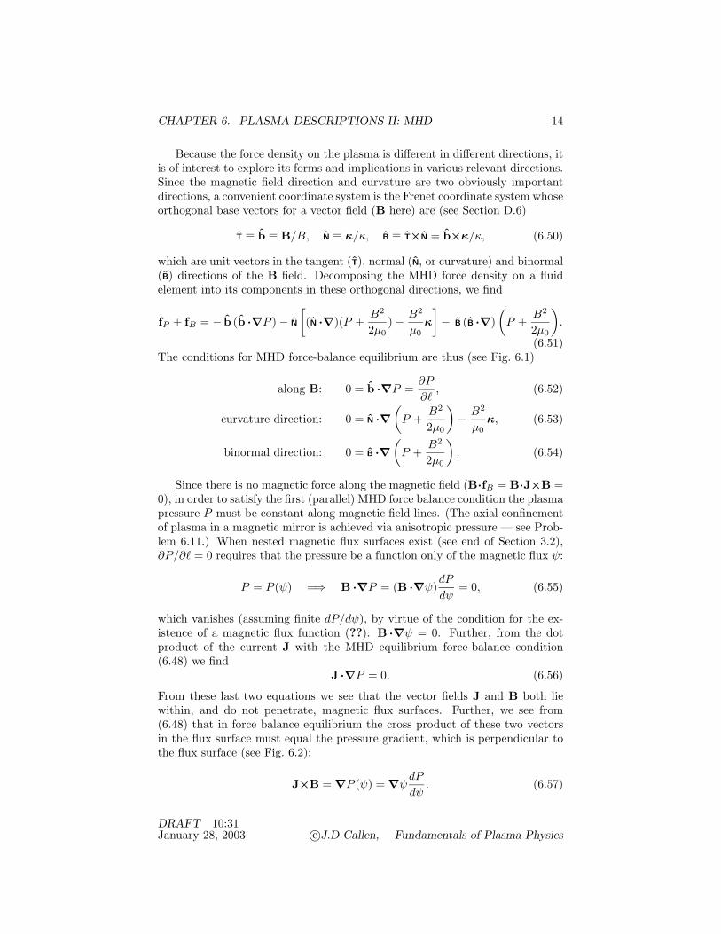
Because the force density on the plasma is different in different directions, itis of interest to explore its forms and implications in various relevant directions.Since the magnetic field direction and curvature are two obviously importantdirections, a convenient coordinate system is the Frenet coordinate system whoseorthogonal base vectors for a vector field (B here) are (see Section D.6)

T ≡ b ≡ B/B, N ≡ κ/κ, B ≡ T×N = b×κ/κ, (6.50)

which are unit vectors in the tangent (T), normal (N, or curvature) and binormal(B) directions of the B field. Decomposing the MHD force density on a fluidelement into its components in these orthogonal directions, we find

fP + fB = − b (b ·∇P )− N

[(N ·∇)(P +

B2

2µ0)− B2

µ0κ

]− B (B ·∇)

(P +

B2

2µ0

).

(6.51)The conditions for MHD force-balance equilibrium are thus (see Fig. 6.1)

along B: 0 = b ·∇P =∂P

∂`, (6.52)

curvature direction: 0 = N ·∇(P +

B2

2µ0

)− B2

µ0κ, (6.53)

binormal direction: 0 = B ·∇(P +

B2

2µ0

). (6.54)

Since there is no magnetic force along the magnetic field (B·fB = B·J×B =0), in order to satisfy the first (parallel) MHD force balance condition the plasmapressure P must be constant along magnetic field lines. (The axial confinementof plasma in a magnetic mirror is achieved via anisotropic pressure — see Prob-lem 6.11.) When nested magnetic flux surfaces exist (see end of Section 3.2),∂P/∂` = 0 requires that the pressure be a function only of the magnetic flux ψ:

P = P (ψ) =⇒ B ·∇P = (B ·∇ψ)dP

dψ= 0, (6.55)

which vanishes (assuming finite dP/dψ), by virtue of the condition for the ex-istence of a magnetic flux function (??): B ·∇ψ = 0. Further, from the dotproduct of the current J with the MHD equilibrium force-balance condition(6.48) we find

J ·∇P = 0. (6.56)

From these last two equations we see that the vector fields J and B both liewithin, and do not penetrate, magnetic flux surfaces. Further, we see from(6.48) that in force balance equilibrium the cross product of these two vectorsin the flux surface must equal the pressure gradient, which is perpendicular tothe flux surface (see Fig. 6.2):

J×B =∇P (ψ) =∇ψdPdψ

. (6.57)



Figure 6.2: In ideal MHD equilibrium the cross product of the current density Jand magnetic field B vectors within a flux surface is equal to∇P = (dP/dψ)∇ψ,which is normal to the flux surface.

Figure 6.3: Pressure P and magnetic energy density B2/2µ0 profiles for: a)β << 1, and b) β ' 1.

When there is no magnetic field curvature, the force balance equilibriumcondition is the same in all directions perpendicular to the magnetic field:

∇⊥(P +

B2

2µ0

)= 0, MHD equilibrium with no B field curvature. (6.58)

To illustrate the implications of this equation, consider the MHD equilibrium ofa localized plasma placed in a uniform magnetic field B = B0b = B0ez, For agiven plasma pressure profile P (x⊥) that varies in directions (x⊥) perpendicularto the magnetic field but does not extend to infinite dimensions, (6.58) yields

∂

∂x⊥

(B2

2µ0

)= − ∂P

∂x⊥=⇒ B(x⊥) = B0

√1− β(x⊥) . (6.59)

Here, we have defined the very important MHD parameter β by

β(x⊥) ≡ P (x⊥)B2

0/2µ0= 4.0× 10−25

( neB2

)[Te(eV) +

nineTi(eV)

],

ratio of plasma pressure to magnetic energy density. (6.60)

Thus, in an MHD equilibrium, for a situation where the magnetic field Bhas no curvature, the plasma digs a magnetic well (region of reduced magneticenergy density) that is just deep enough so that the sum of the plasma pres-sure P and magnetic field energy density B2/2µ0 is constant (at B2

0/2µ0) inall directions perpendicular to the magnetic field. This result is illustrated inFig. 6.3 for a cylindrical plasma where the plasma pressure vanishes at r = a fortwo cases: small β and near unity β. The cylindrical form of (6.59) can also beobtained directly (see Problem 6.14) from the radial force balance equation bycalculating the radial variation of the magnetic field Bz(r) using the azimuthalcomponent of Ampere’s law.

When the magnetic field has curvature, the force balance condition in thenormal (curvature) direction is changed to condition (6.53). Then, the pressure



gradient in the curvature direction can be supported in force balance equilibriumby either the curvature-induced force density (κB2/µ0) or the gradient in themagnetic energy density, or by some combination thereof. When the plasmapressure is low (β << 1), the magnetic field curvature is equal to the gradientof the magnetic field energy density [the situation for a vacuum magnetic field —see (??)] plus a small correction due to the plasma pressure. In the limit wherethe magnetic field curvature is weak (radius of curvature RC much greater thanthe presssure gradient scale length LP ≡ P/|∇⊥P |), the curvature effects aresmall and the variation in magnetic field strength is still approximately as givenin (6.59). [In an axisymmetric tokamak both of these small corrections to (6.59)are unfortunately comparable in magnitude — see Chapter 20.] In the binormaldirection, (6.54) shows that in force balance equilibrium, even with curvaturein the magnetic field B, P + B2/2µ0 is constant in the binormal direction —increases in the plasma pressure P in the binormal direction are balanced bydecreases in magnetic energy density B2/2µ0, like in (6.59).

From the preceding discussion is is clear that the parameter β characterizesthe relative importance of the plasma pressure P versus the magnetic field B.For β << 1 the plasma pressure has a small effect on the MHD equilibriumand the magnetic field structure is approximately that determined from a vac-uum magnetic field representation (??). Also, the diamagnetic current is small(J∗ ' B×∇β/2µ0), as is the (diamagnetic) magnetic susceptibility due to theplasma magnetization produced by the magnetic moments of all the chargedparticles in the plasma gyrating in the magnetic field [χM ' −β/2 — see dis-cussion after (6.12)]. Since the magnetic field is much stronger than the plasmapressure in this regime, it can be used to provide a “magnetic bottle” for plasmaconfinement. In the opposite limit (β >> 1) where the the plasma pressure inmuch larger than the magnetic energy density, in general the plasma “pushes themagnetic field around” and carries it along with its natural motions (pressureexpansion plus flows). A key question for magnetic fusion confinement systemsis the maximum β they can stably confine in equilibrium; the β ∼ 5–10% that isneeded for economically viable deuterium-tritium fusion reactors is apparentlyaccessible in many types of toroidal confinement systems — see Chapter 21.

It is often asked: can a finite pressure plasma support itself entirely with thediamagnetic current and the magnetic field it produces, without any externallyimposed magnetic field? That is, can a plasma organize itself into a closedmagnetic equilibrium that has no connection to the outside world? In orderto examine this question, we consider the equilibrium [∂(ρmV)/∂t = 0] MHDsytem momentum (or force balance) equation obtained from (6.35): ∇·T = 0.Taking the dot product of this equation with the position vector x from thecentroid of the plasma system (to obtain a measure of the MHD system potentialenergy density), we obtain the relation

0 = x ·∇·T =∇· (x ·T)−∇x : T =∇· (x ·T)− tr{T}, (6.61)

in which we have used vector identities (??), (??) and (??). Integrating this



last form over a volume larger than the proposed isolated plasma, we obtain∫©∫S

dS · (x ·T) =∫d3x tr{T}, (6.62)

in which we have used the tensor form of Gauss’ divergence theorem (??) toconvert the volume integral to a surface integral. We now examine the integralson the left and right separately. For the integral on the left we assume negligibleflows (V→ 0) and use (6.37) for T. Then, the integral on the left can be writtenas ∫©∫dS · (x ·T) =

∫©∫dS ·

[x(P +

B2

2µ0

)− (x ·B)B

µ0

]∼ 1r3

r→∞=⇒ 0.

(6.63)As indicated at the end, in the limit of large radial distances r from the isolatedplasma this integral vaishes — because since there are apparently no magneticmonopoles in the universe, the magnetic field B must decrease like that for adipole field does (|B| ∼ 1/r3) so the integrand scales as 1/r5 and when integratedover the surface (|dS| → 4πr2) one finds that the integral decreases at least asfast as 1/r3. Next, we consider the integral on the right. Using the matrixdefinition of the stress tensor T given in (6.45), we find (for an isolated plasmawithin a finite volume V )∫

V

d3x tr{T} =∫V

d3x

(3P +

B2

2µ0

)=⇒ constant. (6.64)

The only way this last integral can vanish, as is required by the combinationof (6.62) and (6.63), is if the plasma pressure P and magnetic energy den-sity B2/2µ0 (both of which are intrinsically positive quantities) vanish. Thus,we have found a contradiction: no isolated finite-pressure plasma can by it-self develop a self-confining magnetic field in force balance equilibrium. Thisproof and analysis is sometimes called a virial theorem (because it results from∫d3x x · f =

∫d3x x ·∇·T = 0) and was first derived by V.D. Shafranov.1

6.4 Boundary Conditions and Shock Relations

The basic subject to be discussed here are the jump conditions at a disconti-nuity in a plasma or at a plasma-vacuum interface, and then the correspondingbounday conditions at a vacuum wall or around coils for a “free-boundary” equi-librium. See Section 3.2 of the Freidberg book. These same equations becomethe shock conditions in a plasma. This section will be written later.

6.5 MHD Dynamics

To explore the elementary dynamical (evolution in time) properties of a plasmain the MHD model, we first assume that the plasma fluid moves with a velocity

1V.D. Shafranov, in Reviews of Plasma Physics, edited by M.A. Leontovich (ConsultantsBureau, New York, 1966), Vol. II.



V(x, t) and determine the changes in the mass density ρm, pressure P and mag-netic field B induced by V. Then, these responses are used in the momentumequation (6.27) which is then solved self-consistently to determine the mass flowvelocity V.

We begin by considering the temporal evolution of the mass density in re-sponse to V, which is governed by (6.25):

∂ρm/∂t|x = −V·∇ρm + ρm∇·V ⇐⇒ dρm/dt = −ρm∇·V, (6.65)

in which we have used the vector identity (??) in obtaining the first form and thetotal time derivative definition in (6.30) in obtaining the second form. Here, asshown in Fig. ??, in the Eulerian (fixed position) picture [first form of (6.65)], theflow causes changes in the mass density at a fixed point by advecting (−V·∇ρm)the mass flow at velocity V into a region of different mass density, or by com-pressibility (∇·V 6= 0) of the flow. In the Lagrangian (moving with fluid ele-ment) picture [second form of (6.65)], the mass density only changes due to thecompressibility of the flow (∇·V 6= 0).

The pressure evolution can be determined from the isentropic form of theMHD equation of state [i.e., (6.29) neglecting the small entropy production dueto joule heating]:

d

dtln

P

ρΓm

=1P

dP

dt− Γρm

dρmdt

=1P

dP

dt+ Γ∇·V = 0, (6.66)

in which (6.65) has been used to obtain the last form. With the total timederivative definition (6.30), this yields

∂P

∂t= −V·∇P − ΓP∇·V = −V·∇P − c2S ρm∇·V (6.67)

in whichcS ≡

√ΓP/ρm, MHD sound speed (m/s). (6.68)

Thus, like the mass density, the plasma pressure changes in MHD are due toadvection (V·∇P ) and flow compression (∇·V 6= 0). The presence of the soundspeed in the last form of (6.67) shows that the compressiblity of the flow leads topressure changes that move at the MHD sound speed through the plasma. Thus,the fluid motion at velocity V causes advection and compressibility changes inthe mass density ρm and plasma pressure P , which are scalar quantities.

Note that the MHD sound speed is different from the ion acoustic speed(??) in Section 1.4 — because in a MHD description both the electrons and ionshave fluidlike (inertial) responses whereas for ion acoustic waves while the ionshave a fluidlike response the electrons respond adiabatically. Unfortunately,inplasma physics the same symbol is usually used for both wave speeds — whichis meant is usually clear from the context. Also note that for most plasmaswith comparable electron and ion temperatures these two speeds are close inmagnitude.

The next question is: what is the effect of the fluid motion on the magneticfield B(x, t), which is a vector field? Physically, we know that plasmas have



a very high electrical conductivity (low resistivity). In the ideal MHD modelwe set the resistivity to zero and hence effectively assume infinite electricalconductivity; thus, the plasma is a “superconductor” in ideal MHD. From theproperties of a superconducting wire of finite cross-section, we know that themagnetic field is “frozen” into it and moves with the wire as it is moved. Thus,we can intuitively anticipate that a fluid element in our superconducting idealMHD plasma will carry the magnetic field (or at least the bundle of magneticfield lines penetrating it) with it wherever it moves — and will always contain thesame amount of magnetic flux (number of field lines2). We can also anticipatethat the addition of resistivity in the resistive MHD model will allow someslippage of the magnetic field lines relative to the fluid element.

We now develop mathematical representations of the idea that the magneticfield is mostly frozen into an MHD fluid element and moves with it. Considerthe time derivative of the magnetic flux Ψ ≡

∫∫S

B · dS [see (??)] though anopen surface S in the fluid that moves with the fluid at velocity V:

dΨdt

=d

dt

∫∫S

B · dS =∫∫S

[dBdt· dS + B · d

dt(dS)

]. (6.69)

The total time derivative is appropriate here because we are seeking the changein the magnetic flux penetrating a (changing) surface whose boundary is dis-torted in time as it moves with the fluid velocity V(x, t), which is in generalnonuniform. The time derivative of the (vectorial) differential surface area dSrepresents changes due to changes in its constituent differential line elementsinduced by the nonuniform flow — see Section D.4. Using (??) for this timederivative and the definition of the total time derivative in (6.30), we find

dΨdt

=∫∫S

[(∂B∂t

+ V·∇B)

+ B (∇·V)−B ·∇V]· dS

=∫∫S

[∂B∂t−∇×(V×B)

]· dS, (6.70)

in which we have used vector identity (??) and the Maxwell equation ∇·B = 0in going from the first to the second line.

For the evolution of the magnetic field B we use Faraday’s law (6.31) togetherwith the MHD Ohm’s law (6.28) to specify the electric field E:

∂B∂t

= −∇×E = ∇×(V×B)−∇×ηJ ' ∇×(V×B) +η

µ0∇2B

MHD magnetic field evolution. (6.71)

Here, in the last, approximate form we have used J =∇×B/µ0 (Ampere’s law),neglected ∇η for simplicity, and used the vector identity (??) and the Maxwell

2While magnetic field lines do not really exist since their properties cannot be measured,they are a useful concept for visualizing the behavior of the magnetic field B.



equation∇·B = 0. Substituting this magnetic field evolution into (6.70), usingAmpere’s law for J again and Stokes’ theorem (??), we finally obtain

dΨdt

= −∫∫S

dS · ∇×ηJ = −∮C

d` · ηµ0

B. (6.72)

In ideal MHD where η → 0, this becomes

dΨdt

= 0, ideal MHD frozen flux theorem.3 (6.73)

Thus, in the absence of resistivity the magnetic flux (number of field lines)through an open surface that moves with the fluid velocity V is “frozen” intothe fluid and hence constant: the magnetic field moves with the superconductingideal MHD fluid just as we wanted to prove! The key ingredient in this derivationis the V×B term in the MHD Ohm’s law. It led to the ∇×(V×B) term inthe magnetic field evolution equation (6.71) and causes the magnetic field to becarried along with the ideal MHD fluid. Hence, this∇×(V×B) term representsthe advection of the vector field B by the flow velocity V; note that this vectorfield advection operator is different in structure from the advection operatorfor scalar quantities such as the mass density (−V·∇ρm). Since the MHDOhm’s law is an approximation to the electron momentum balance equation, itis fundamentally the electron fluid into which magnetic field is frozen (despitethe fact that the advection is induced by the overall plasma mass flow velocityV).

By taking the limit of an infintesimally small surface S in the precedingderivation, one can show that an individual magnetic field line is carried alongwith the superconducting ideal MHD plasma. This can also be shown directlyby examining the conditions under which the time derivative of the definitionsof magnetic field lines vanish — see Problems 6.15 and 6.16. However, it isimportant to note that all these derivations have some ambiguity because thelabeling of a magnetic field line is not unique [see discussion after (??)] andthe properties of magnetic field lines cannot be measured. Thus, while we canmark infintesimal elements of a fluid (e.g., with radioactive nuclei or fluorescingpartially ionized atoms), and know that the magnetic field is frozen into the idealMHD fluid elements as they move, the association with a particular magneticfield line from one instant in time to the next is not unique. The “frozen flux”methodology provides a prescription for labeling field lines as they move. Whileit is not a unique prescription, it represents a very important tool for visualizingthe motion of magnetic fields in a moving plasma in the MHD model.

The frozen flux theorem provides a very strong constraint on the motionsof the magnetic field in an ideal MHD plasma. In particular, in this modeladjacent magnetic field lines and flux bundles that are originally adjacent toeach other will forever remain adjacent. Also, magnetic flux bundles and fluid

3This theorem is also known as the Alfven frozen flux theorem. It is the magnetic fieldanalogue of the Kelvin circulation theorem (??) for the constancy of the circulation or vorticityflux in a vortex in an inviscid neutral fluid.



Figure 6.4: Possible MHD evolution of a set of field lines in a sheared slabmagnetic field model: a) initial sheared magnetic field equilibrium, b) sinusoidalperturbation in ideal MHD (η = 0), and c) resistive MHD (η 6= 0) with magneticfield reconnection into magnetic island structures.

elements are tied together, cannot break up or tear, and cannot interchangepositions relative to each other. Thus, as illustrated in Figure 6.4, in the idealMHD model the topology of magnetic field lines and flux surfaces is conserved— nested magnetic flux surfaces remain forever nested (even though their shapemay become highly distorted), and plasma in regions “inside” (or “outside”) agiven magnetic flux surface remain inside (outside) forever. The inclusion ofresistivity in the MHD model allows diffusion of the magnetic field relative tothe plasma, and hence reconnection of the magnetic field lines and changes inthe magnetic topology — for example by forming a magnetic island such asindicated in Figure 6.4c. In section 6.7 we discuss the relative importance ofresistivity in MHD analyses of plasmas.

The most convenient form of the MHD momentum equation (6.27) for dy-namical analyses uses the middle form of the force density fB in (6.46) and isgiven by

ρmdVdt

= −∇(P +

B2

2µ0

)+

(B ·∇)Bµ0

. (6.74)

Note that we have now reduced the full MHD equation set (6.25)–(6.44) tojust three (or seven component) equations — the scalar pressure equation in(6.67), the vector magnetic field evolution equation in (6.71) and this last vectormomentum equation (6.76). These equations are usually all we need to describethe linear and nonlinear dynamics of plasmas in the MHD model. [The massdensity equation (6.65) is only needed when the equilibrium mass density isinhomogeneneous.] Note that for these MHD dynamical model equations thecharge continuity equation ∇· J = 0 is automatically satisfied by our havingused Ampere’s law to replace the current J with ∇×B/µ0, which is divergencefree. Also, the electric field E does not appear because it was replaced by−V×B + ηJ using the MHD Ohm’s law.

6.6 Alfven Waves

To illustrate the fundamental wave responses of plasmas in the MHD model(Alfven waves — named after their discoverer), we consider plasma responsesto small perturbations in the simplest possible plasma and magnetic field model.Namely, for the equilibrium we consider a uniform, nonflowing (V0 = 0) plasmain an infinite, homogeneous magnetic field B0 = B0ez = B0b. This model



trivially satisfies the MHD equilibrium force balance condition (6.48) sinceµ0J0 = ∇×B0 = 0 and ∇P = 0 because both the equilibrium magnetic fieldB0 and pressure P0 are uniform in space. For perturbed responses we assume

ρm = ρm0 + ρm, P = P0 + P , V = V, B = B0 + B, (6.75)

in which the zero subscript indicates equilibrium quantities and the tilde overquantities indicates perturbed variables. Decomposing the perturbed mag-netic field into its parallel [B‖ = b(b · B) = B‖b] and perpendicular [B⊥ ≡−b×(b×B)] components, we find the square of the magnetic field strength Bis

B2 ≡ (B0 + B) · (B0 + B) = B20 + 2B0B‖+ B2

‖ + |B⊥|2 ' B20 + 2B0B‖. (6.76)

We will use the last expression, which is the linearized form (i.e., it neglectsterms that are second order in the perturbation amplitudes).

Substituting the equilibrium plus perturbed quantities in (6.75) and (6.76)into the ideal MHD equations for the evolution of the pressure (6.67), flowvelocity (6.74) and magnetic field [(6.71) with η → 0] and linearizing (neglectsecond and higher order terms in the perturbation amplitudes), we obtain

∂P

∂t= −ΓP0∇·V, (6.77)

ρm0∂V∂t

= −∇(P +

B0B‖µ0

)+

1µ0

(B0·∇)B, (6.78)

∂B∂t

= ∇×(V×B0) = −B0(∇·V) + (B0·∇)V. (6.79)

In the last equation we used vector identity (??) and set to zero terms involvinggradients of the homogeneous equilibrium magnetic field B0. Equations for theparallel and perpendicular components of the magnetic field are obtained fromthe corresponding projections of the magnetic field evolution equation:

∂B‖/∂t = −B0(∇·V) + (B0·∇)V‖, (6.80)

∂B⊥/∂t = (B0·∇)V⊥. (6.81)

These equations can be combined into a single (vector) equation by taking thepartial derivative of the perturbed momentum equation (6.78) and substitutingin the needed partial derivatives from the other equations (see Problem 6.20):

∂2V∂t2

= (c2S + c2A)∇(∇·V) + c2A[∇2‖V⊥ −∇⊥∇‖V‖ − b∇‖(∇·V)] (6.82)

in which

cA ≡B0√µ0ρm0

' 2.2× 1016 B0√niAi

m/s, Alfven speed. (6.83)



Here, Ai ≡ mi/mp is the atomic mass value of the ions, the perpendicular (⊥)and parallel (‖) subscripts indicate the respective components of the quantitiesas defined in (??)–(??). The magnitude of the Alfven speed can be appreciatedby noting its relationship to the sound speed defined in (6.68):

c2Sc2A

=ΓP0/ρm0

B2/µ0ρm0=

Γ2β. (6.84)

Thus, for β < 1 the Alfven speed is a factor of about 1/√β greater than the

MHD sound speed.While (6.82) clearly has a wavelike structure, it is a quite complicated and

anisotropic wave equation. We consider here only some special cases to illustratethe basic waves involved. (Section 7.6* provides a comprehensive analysis.)

First, consider waves propagating purely perpendicular to the magnetic fieldby setting ∇‖ = 0. Then, taking the divergence of (6.82) we obtain[

∂2

∂t2− (c2A + c2S)∇2

⊥

](∇⊥· V⊥) = 0 =⇒ ω2 = k2

⊥(c2A + c2S),

compressional Alfven waves. (6.85)

This wave equation describes “fast” compressional Alfven waves. In the lastform we assumed a wave-like response V⊥ ∼ exp[i(k·x−ωt)] to obtain the wavedispersion relation. Compressional Alfven waves propagate perpendicular tothe magnetic field with a wave phase speed given by Vϕ⊥ ≡ ω/k⊥ =

√c2A + c2S ,

which is the fastest MHD wave phase speed. These waves propagate by per-pendicular flow compression (∇⊥ · V⊥ 6= 0) and also involve magnetic fieldcompression [B‖ 6= 0 — see (6.80)] and pressure perturbations [P 6= 0 — see(6.85)]. Adding the pressure perturbation (6.77) and B0/µ0 times the magneticperturbation (6.80) with ∇‖ = 0, one can show that

∂2

∂t2

(P +

B0B‖µ0

)= −(c2A + c2S)∇⊥· ρm0

∂V⊥∂t

= (c2A + c2S)∇2⊥

(P +

B0B‖µ0

)(6.86)

in which for the last form we have used (6.78) with ∇‖ = 0. Thus, the compress-ibility in the perpendicular flow also causes the sum of the perturbed pressureand magnetic field energy density to satisfy a compressional Alfven wave equa-tion. Physically, as can be noted from the importance of the perpendicularcomponent of (6.78) in these waves, the compressional Alfven waves are theresponses of the plasma to imbalances in the perpendicular (to B) force balancein the plasma. Thus, on “equilibrium” time scales (after these wave responseshave propagated away), MHD plasma responses will be in radial force balanceequilibrium and not have any driving sources for compressional Alfven waves:

J0×B0 =∇⊥P0, ∇⊥· V⊥ = 0, P +B0B‖/µ0 = 0. (6.87)

These are the lowest order conditions for equilibria and perturbations in anMHD plasma (even in inhomogeneous magnetic fields — see Chapter 21); they



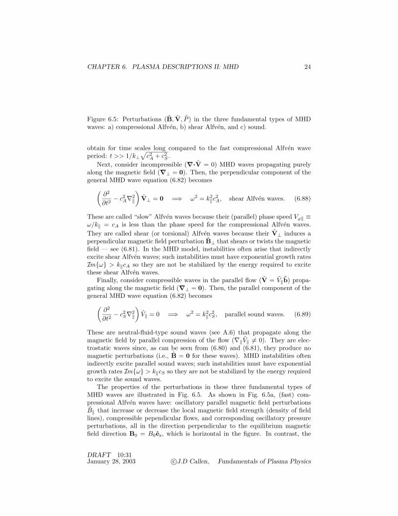
Figure 6.5: Perturbations (B, V, P ) in the three fundamental types of MHDwaves: a) compressional Alfven, b) shear Alfven, and c) sound.

obtain for time scales long compared to the fast compressional Alfven waveperiod: t >> 1/k⊥

√c2A + c2S .

Next, consider incompressible (∇·V = 0) MHD waves propagating purelyalong the magnetic field (∇⊥ = 0). Then, the perpendicular component of thegeneral MHD wave equation (6.82) becomes(

∂2

∂t2− c2A∇2

‖

)V⊥ = 0 =⇒ ω2 = k2

‖c2A, shear Alfven waves. (6.88)

These are called “slow” Alfven waves because their (parallel) phase speed Vϕ‖ ≡ω/k‖ = cA is less than the phase speed for the compressional Alfven waves.They are called shear (or torsional) Alfven waves because their V⊥ induces aperpendicular magnetic field perturbation B⊥ that shears or twists the magneticfield — see (6.81). In the MHD model, instabilities often arise that indirectlyexcite shear Alfven waves; such instabilities must have exponential growth ratesIm{ω} > k‖cA so they are not be stabilized by the energy required to excitethese shear Alfven waves.

Finally, consider compressible waves in the parallel flow (V = V‖b) propa-gating along the magnetic field (∇⊥ = 0). Then, the parallel component of thegeneral MHD wave equation (6.82) becomes(

∂2

∂t2− c2S∇2

‖

)V‖ = 0 =⇒ ω2 = k2

‖c2S , parallel sound waves. (6.89)

These are neutral-fluid-type sound waves (see A.6) that propagate along themagnetic field by parallel compression of the flow (∇‖V‖ 6= 0). They are elec-trostatic waves since, as can be seen from (6.80) and (6.81), they produce nomagnetic perturbations (i.e., B = 0 for these waves). MHD instabilities oftenindirectly excite parallel sound waves; such instabilities must have exponentialgrowth rates Im{ω} > k‖cS so they are not be stabilized by the energy requiredto excite the sound waves.

The properties of the perturbations in these three fundamental types ofMHD waves are illustrated in Fig. 6.5. As shown in Fig. 6.5a, (fast) com-pressional Alfven waves have: oscillatory parallel magnetic field perturbationsB‖ that increase or decrease the local magnetic field strength (density of fieldlines), compressible pependicular flows, and corresponding oscillatory pressureperturbations, all in the direction perpendicular to the equilibrium magneticfield direction B0 = B0ez, which is horizontal in the figure. In contrast, the



(slow) shear Alfven waves (Fig. 6.5b) have: oscillatory perpendicular magneticfields B⊥ and oscillatory perpendicular flows V⊥ along the magnetic field, butno pressure perturbation (because these perurbed flows are incompressible). Fi-nally, as shown in Fig. 6.5c, the parallel sound waves have: no magnetic fieldperturbation (because they are electrostatic), an oscillatory compressible paral-lel flow V‖ and corresponding pressure P perturbations along the magnetic fielddirection.

In the more general case of propagation of MHD waves at arbitrary anglesto the magnetic field direction, these three types of waves become coupled (seeSection 7.6). These waves also become coupled in inhomogeneous magnetic fields— because the parallel and perpendicular directions vary spatially. Nonetheless,the basic wave characteristics we have discussed are usually still evident in thesemore complicated situations.

6.7 Magnetic Field Diffusion in MHD

In order to examine the effect of electrical resistivity on a plasma in the MHDmodel, consider first the evolution of the magnetic field in (6.71) without theadvection term:

∂B∂t

=η

µ0∇2B, magnetic field diffusion equation. (6.90)

This equation describes the diffusion (see Section A.5) of the magnetic field(both its magnitude and directional components) that is caused by the electricalresistivity of a plasma. The diffusion coefficient is

Dη =η

µ0=

meνeµ0nee2

' 1.4× 103

(Zi

Te(eV)]3/2

)(ln Λ17

)m2/s

magnetic field diffusivity. (6.91)

Phenomenologically, since we can write Dη = νe(c/ωpe)2, magnetic field diffu-sion can be thought of [via D ∼ (∆x)2/∆t — see (??)] as emanating from arandom walk process in which magnetic field lines step a collisionless skin depth(∆x ∼ c/ωpe) in an electron collision time (∆t ∼ 1/νe). The relative magnitudeof the magnetic field diffusivity can be ascertained from its relationship to theclassical diffusivity D⊥ defined in (??):

D⊥η/µ0

=νe%

2e

νe(c/ωpe)2

(Te + Ti

2Te

)=ne(Te + Ti)c2ε0B2

=β

2. (6.92)

Thus, for a plasma with β < 1 particles diffuse classically across magneticfield lines slower than the magnetic field lines themselves diffuse relative tothe plasma! However, in most plasmas of interest microscopic turbulence inplasmas causes an anomalous perpendicular transport that is rapid comparedto the magnetic field diffusion; hence one can usually consider the magnetic fieldto be stationary for calculations of anomalous transport.



To illustrate the spatial and temporal scale lengths involved in magnetic diff-ision, consider the distance an electromagnetic wave can penetrate (see Section1.5) into a resistive medium in which the magnetic field behavior is governed by(6.90). For wavelike perturbations B ∼ exp[i(k·x− ωt)], the diffusion equationbecomes

−iωB = −k2(η/µ0)B =⇒ k =√iωµ0/η = (1 + i)

√(ω/2)(µ0/η). (6.93)

To use the analysis of Section 1.5, we identify this complex wavenumber k asthe transmitted wavenumber kT in (??). Thus, an electromagnetic wave will bedissipated and damped exponentially, as it oscillates spatially (due to Re{kT })and propagates into a resistive medium, with a characteristic decay length of

δη ≡1

Im{(kT }=√

2ω

η

µ0, resistive skin depth. (6.94)

It is called a “skin” depth because of its analogy with the problem of deter-mining how far an oscillating magnetic field (e.g., due to 60 Hz AC electricity)penetrates into a cylindrical wire of finite radius. This skin depth formula isappropriate for radian frequencies ω < νe, while the collisionless skin depth for-mula (??) is appropriate for higher frequencies — see Problem 6.25. For Te =2000 eV, which gives η/µ0 ' 0.016 m2/s (close to the resistivity of copper atroom temperature of η/µ0 ' 0.135 m2/s), the resistive skin depth ranges from0.07 mm for f = ω/2π = 104 Hz (ω = 2π × 104) to about 1 cm for 60 Hz.

Another way of illustrating the temporal behavior of magnetic field diffusionin a magnetized plasma is to ask: on what time scale τ will a magnetic fieldcomponent diffuse away from being localized to a region of width L⊥? Becausefor diffusive processes the diffusion coefficient scales with spatial and temporalsteps as D ∼ (∆x)2/∆t ∼ L2

⊥/τ (see Appendix A.5), we can estimate phe-nomenologically that τ ∼ L2

⊥/(η/µ0). One often considers a cylindrical modelconsisting of a column of magnetized plasma with radius a that initially carriesan axial current. For such a cylindrical model the resistivity-induced decay timeof the current (and induced azimuthal magnetic field) is (see Section A.5)

τη 'a2

6 η/µ0, resistive skin diffusion time. (6.95)

Here, the numerical factor of 6 is a cylindrical geometry factor which more pre-cisely is the square of the first zero of the J0 Bessel function: j2

0,0 ' 2.4052 ' 5.78— see Appendix A.5 and (??). However, the additional accuracy is unwarrantedboth because of the approximations involved in the simple model used to deriveτη and because of the intrinsic accuracy of the electrical resistivity (' 1/ ln Λ ∼5–10%). For a plasma of radius a = 0.3 m with Te = 2000 eV, which givesη/µ0 ' 0.016 m2/s, the skin time is τη ∼ 1 s.

Finally, we discuss the relative importance of the two contributions to mag-netic field evolution (6.71) in the MHD model: advection of the magnetic fieldby ∇×(V×B), and resistive diffusion by (η/µ0)∇2B. The relative importance



of these two terms is indicated by the scaling properties of their ratio:

S =|∇×(V×B)||(η/µ0)∇2B| ∼

cA/L‖(η/µ0)/a2

' 1.6× 1013 a2B[Te(eV)]3/2

L‖Zi√niAi

(17

ln Λ

),

Lundquist number.4 (6.96)

Here, we have taken the typical velocity to be the Alfven speed cA and assumedscale lengths L‖ [e.g., periodicity scale length along B — see (6.81)] for theadvection process and a (e.g., plasma radius) for the magnetic diffusion. TypicalLundquist numbers range from 102 for cold, resistive plasmas, to 105–1010 forthe earth’s magnetosphere and magnetic fusion experiments, to 1010–1014 forthe sun’s corona and astrophysical plasmas.

Because the Lundquist number is large for almost all magnetized plasmasof interest (and extremely large for high temperature plasmas), one might betempted to just set the resistivity to zero (S → ∞) and always use the idealMHD model. Indeed, throughout most of a plasma the magnetic field is frozeninto and moves with the plasma fluid. However, a small resistivity can bevery important in resistive boundary layers. The boundary layers occur inthe vicinity of magnetic field lines where the parallel derivative (B0·∇)V⊥ in(6.81) vanishes so the B⊥ evolution becomes dominated by resistive evolutionof B⊥, rather than by advection. The width of these resistive boundary layersscales inversely with a fractional power of the Lundquist number (S−1/3 orS−2/5) and hence is not negligible — see Chapter 22. Since resistivity allows themagnetic field lines to slip relative to the plasma fluid, they relax (in the resistivelayers) the frozen flux constraint and thereby allow new types of instabilities— resistive MHD instabilities, which are described in Chapter 22. Since theresistivity only relaxes the frozen flux constraint in thin layers, resistive MHDinstabilities grow much slower (by factors of S−1/3 or S−3/5) than ideal MHDinstabilities. However, resistive MHD instabilities are quite important, becausethey can lead to turbulent plasma transport (see Section 25.3) and becausein these narrow resistive boundary layers the magnetic field lines can tear orreconnect and thereby lead to changes in the magnetic topology (see Section22.3). For example, they can nonlinearly evolve into a magnetic island structurelike that shown in Fig. 6.4c.

6.8 Which Plasma Description To Use When?

In this section we discuss which types of plasma descriptions are used for describ-ing various types of plasma processes in magnetized plasmas. This discussionalso serves as an introduction to most of the subjects that will be covered in theremainder of the book. The basic logic is that the fastest, finest scale processes

4Many plasma physics textbooks refer to this as the “magnetic Reynolds number.” How-ever, S is the ratio of linear advection to a dissipative process rather than the ratio of nonlinearadvection to a dissipative process, as the neutral fluid Reynolds number is — see (??). Wewill call S the Lundquist number to avoid the implication that this dimensionless number isindicative of nonlinear processes that always lead to turbulence when it is large.



require kinetic descriptions, but then over longer time and length scales morefluidlike, macroscopic models become appropriate. Also, the “equilibrium” ofthe faster time scale processes often provide constraint conditions for the longertime scale, more macroscopic processes.

In a magnetized plasma there are many more relevant parameters, and theirrelative magnitudes and consequences can vary from one application to another.Thus, to provide a table similar to Table ?? for magnetized plasmas, we need tospecify the parameters for a particular application. We will choose parameterstoward the edge (r/a = 0.7) of a typical 1990s “large-scale” tokamak plasma(e.g., the Tokamak Fusion Test Reactor: TFTR): Te = Ti = 1 keV, ne = 3×1019

m−3, B = 4 T, deuterium ions, Zeff = 2, L‖ = R0q ' 6 m, a = 0.8 m, Lp = 0.5m. In a magnetized plasma the unmagnetized phenomena listed in Table ??still occur; however, their effects only influence responses along the magneticfield direction. Parameters for the gyromotion, bounce motion and drift motionof charged particles in this tokamak magnetic field structure are approximatelythe same as those indicated in (??) and (??).

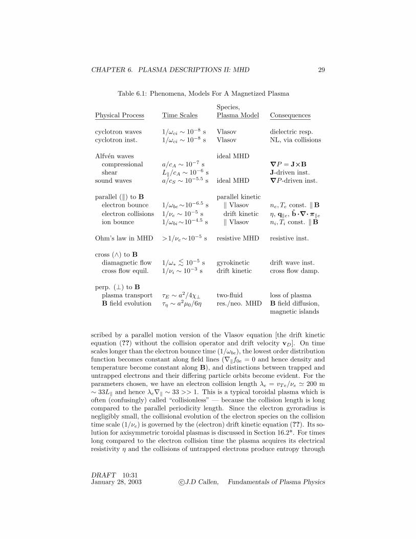
Table 6.1 presents an outline of magnetized-plasma-specific plasma phenom-ena, and their relevant time scales, appropriate models and possible conse-quences for the tokamak plasma parameters indicated in the preceding para-graph. In it time scales are indicated in “half order of magnitudes” (100.5 =3.16 · · · ∼ 3). As indicated, the fastest magnetic-specific process in magnetizedplasmas is the gyromotion of particles about the magnetic field, for which the ap-propriate model is the Vlasov equation. The ion gyromotion leads to cyclotron(Bernstein) waves, finite ion gyroradius (FLR) effects and a perpendicular di-electric response (Sections 7.5, 7.6). There are of course also electron cyclotronmotion and waves. The propagation of (electron and ion) cyclotron-type wavesin plasmas and their use for wave heating of magnetized plasmas are discussedin Chapters 9 and 10. If the electron or ion distribution function is peaked at anonzero energy (so ∂f0/∂ε > 0), it can lead to cyclotron instabilities (Chapter18) whose nonlinear evolution to a steady state or bursting situation is oftendetermined by collisions (Section 24.1).

The next fastest time scales are typically those associated with the the Alfvenwave and sound wave frequencies which are described by the ideal MHD model:(6.25)–(6.39) with η → 0. As indicated in Table 6.1, in the usual situationwhere compressional Alfven waves are stable, their effect is to impose radial (⊥to B) force balance equilbrium [(6.48) and Chapter 20] on the plasma and lowerfrequency perturbations in the plasma. The shear Alfven and sound wavescan lead to virulent macroscopic current-driven (kink) and pressure-gradient-driven (interchange) instabilities (Chapter 21). The nonlinear consequencesof an ideal MHD instability is often dramatic movement or catastrophic lossof the plasma in a few to ten instability growth times; hence most magneticconfinement systems are designed to provide ideal MHD stability for the plasmasplaced in them.

Next, we turn to the sequentially slower particle and plasma motions along(‖), across (∧) and perpendicular (⊥) to the magnetic field B. The fastestmotion along a magnetic field line is the electron bounce motion, which is de-



Table 6.1: Phenomena, Models For A Magnetized Plasma

Species,Physical Process Time Scales Plasma Model Consequences

cyclotron waves 1/ωci ∼ 10−8 s Vlasov dielectric resp.cyclotron inst. 1/ωci ∼ 10−8 s Vlasov NL, via collisions

Alfven waves ideal MHDcompressional a/cA ∼ 10−7 s ∇P = J×Bshear L‖/cA ∼ 10−6 s J-driven inst.

sound waves a/cS ∼ 10−5.5 s ideal MHD ∇P -driven inst.

parallel (‖) to B parallel kineticelectron bounce 1/ωbe∼10−6.5 s ‖ Vlasov ne, Te const. ‖Belectron collisions 1/νe ∼ 10−5 s drift kinetic η, q‖e, b ·∇·π‖eion bounce 1/ωbi∼10−4.5 s ‖ Vlasov ni, Ti const. ‖B

Ohm’s law in MHD >1/νe∼10−5 s resistive MHD resistive inst.

cross (∧) to Bdiamagnetic flow 1/ω∗ <∼ 10−5 s gyrokinetic drift wave inst.cross flow equil. 1/νi ∼ 10−3 s drift kinetic cross flow damp.

perp. (⊥) to Bplasma transport τE ∼ a2/4χ⊥ two-fluid loss of plasmaB field evolution τη ∼ a2µ0/6η res./neo. MHD B field diffusion,

magnetic islands

scribed by a parallel motion version of the Vlasov equation [the drift kineticequation (??) without the collision operator and drift velocity vD]. On timescales longer than the electron bounce time (1/ωbe), the lowest order distributionfunction becomes constant along field lines (∇‖f0e = 0 and hence density andtemperature become constant along B), and distinctions between trapped anduntrapped electrons and their differing particle orbits become evident. For theparameters chosen, we have an electron collision length λe = vTe/νe ' 200 m∼ 33L‖ and hence λe∇‖ ∼ 33 >> 1. This is a typical toroidal plasma which isoften (confusingly) called “collisionless” — because the collision length is longcompared to the parallel periodicity length. Since the electron gyroradius isnegligibly small, the collisional evolution of the electron species on the collisiontime scale (1/νe) is governed by the (electron) drift kinetic equation (??). Its so-lution for axisymmetric toroidal plasmas is discussed in Section 16.2*. For timeslong compared to the electron collision time the plasma acquires its electricalresistivity η and the collisions of untrapped electrons produce entropy through



“neoclassical” heat conduction (q‖e) and parallel viscosity (b ·∇·π‖e) — seeChapter 16. Similarly, the lowest order ion distribution function, density andtemperature become constant along magnetic field lines for time scales longerthan the ion bounce time (1/ωbi) and their collisional effects (in relaxing crossflows within a magnetic flux surface) become evident on the ion collision timescale (1/νi).

The plasma exhibits an electrical resistivity for time scales longer than theelectron collision time (1/νe). Its introduction into MHD leads to the resistiveMHD model: (6.25)–(6.39). Since the introduction of resistivity relaxes theideal MHD frozen flux constraint (in narrow layers), it can lead to resistiveMHD instabilities related to their ideal MHD counterparts (kink → tearing,∇P -driven “interchange” → resistive interchange), which, however, grow moreslowly and hence are less virulent — see Chapter 22.

The next set of phenomena concern the effects of particle drifts and plasmaspecies flows in the cross direction (∧ — perpendicular to B and within a fluxsurface if it exists). On this time scale a global (as opposed to local) descriptionof the magnetic field is usually required. The diamagnetic flows of electronsand ions lead to drift-wave-type oscillations (Sections 7.4* and 8.6*) and insta-bilities (Section 23.3*). Since these “universal” instabilities involve modes withsignificant ion gyroradius (FLR) effects (%i∇⊥ ∼ k⊥%i ∼ 1), the gyrokineticequation is used to describe their nonlinear evolution into microsopic plasmaturbulence (Chapter 25) that leads to anomalous radial transport (Chapter 26)of the plasma. On the same time scales the combination of the E×B and dia-magnetic flows come into “equilibrium” (a steady state saturation or boundedcyclic behavior); flow components within a magnetic flux surface in directionsin which the magnetic field is inhomogeneous (e.g., the poloidal direction in anaxisymmetric tokamak) are damped on the ion collision time scale (1/νi) — seeSection 16.3*. Steady-state net radial transport fluxes can only be properly cal-culated after the flows within magnetic flux surfaces are determined and relaxedto their equilibium values. Also, in determining transport fluxes it is implicitlyassumed that nested magnetic flux surfaces exist and that “radial” transport isto be calculated relative to them.

Finally, we reach the transport time scales on which the plasma and mag-netic field diffuse radially out of the plasma confinement region, and radiation(Chapter 14) can be significant. Plasma transport (relative to the magneticfield) is usually modeled with two-fluid equations averaged over magnetic fluxsurfaces to yield equations that govern the transport of plasmas perpendicularto magnetic flux surfaces — see Chapter 17. However, the radial particle andheat diffusion coefficients D⊥, χ⊥ are usually assumed to be the sum of thoseproduced by anomalous transport (Chapter 26) and those due to classical [(??),(??) and Chapter 15] and neoclassical (Chapter 16) transport processes. For acylindrical-type plasma model the characteristic time scale for the usally dom-inant plasma energy loss is (see Section 17.3) approximately τE ∼ a2/4χ⊥ inwhich a is the plasma radius; for the plasma parameters we are considering itis of order 0.1 s. Simultaneously, the magnetic field is diffusing. The character-istic time scale for diffusive transport of magnetic field lines out of a cylindrical



plasma is τη ∼ a2/(6η/µ0); for the plasma parameters we are considering it is oforder 1 s. If resistive or neoclassical MHD tearing-type instabilities are present,they can reconnect magnetic field lines on rational magnetic flux surfaces andevolve nonlinearly by forming magnetic islands which grow (to saturation ortotal plasma loss) on a fraction (∼ 0.1) of the magnetic field diffusion time scaleτη. Since the magnetic field typically diffuses more slowly than energy is lost viaanomalous transport (i.e., τη >> τE or η/µ0 << χ⊥), it is usually reasonableto assume that the magnetic field is stationary and the plasma moves relativeto it via Coulomb-collision-induced or anomalous plasma transport processes.

REFERENCES AND SUGGESTED READING

The MHD description of a plasma and its properties are presented in

Schmidt, Physics of High Temperature Plasmas (1966,1979), Chapts. 3,4 [?]

Krall and Trivelpiece, Principles of Plasma Physics (1973), Chapts. 2.3 [?]

Freidberg, Ideal Magnetoydrodynamics (1987) [?]

Sturrock, Plasma Physics, An Introduction to the Theory of Astrophysical, Geo-physical & Laboratory Plasmas (1994), Chapts. 11,12 [?]

Hazeltine and Waelbroeck, The Framework of Plasma Physics (1998), Chapts.3–6 [?]

Bateman, MHD Instabilities (1980) [?]

Biskamp, Nonlinear Magnetohydodynamics (1993) [?]

The neoclassical MHD model for axisymmetric toroidal plasmas is described in

J.D. Callen, W.X. Qu, K.D. Siebert, B.A. Carreras, K.C. Shaing and D.A.Spong,“Neoclassical MHD Equations, Instabilities and Transport in Tokamaks,”in Plasma Physics and Controlled Nuclear Fusion Research 1986 (IAEA, Vienna,1987), Vol. II, p. 157 [?]

PROBLEMS

6.1 Use the definition of the pressure in (??) with vr ≡ v − V to show that theisotropic pressure of a species in the center-of-mass frame (V) of an MHD plasmais

pCMs = ps + (nsms/3)|Vs −V|2. /∗

6.2 Show that the plasma momentum equation (6.6) obtained by adding the electronand ion momentum equations is exact (i.e., it does not involve an me/mi << 1approximation). [Hint: To obtain the inertia term on the left it is easiest to use(??) for the electron and ion momentum equations. Also, first show that∑

s

msnsVsVs = ρmVV +∑s

msns(Vs −V)(Vs −V)

in which V is the MHD mass flow velocity defined in (6.19).] //*

6.3 Evaluate ∇· JD and show that it is equal to ∇· J∗, and to the terms on theright of (6.16). Explain the physical significance of the equality of these twoquantities. //*



6.4 Multiply the electron and ion momentum balance equations (??) by qe/me andqi/mi and add them to obtain the exact generalized Ohm’s law

∂J

∂t+∇· (JV + VJ− ρqVV) = ε0ω

2p

{E + V×B−

(J‖

σ‖+

J⊥σ⊥

)− (1− Zime/mi)J×B−∇· [PCM

e − Zi(me/mi)PCMi ]

(1 + Zime/mi)nee

}in which PCM

s ≡ psI + πs + nsms(Vs − V)(Vs − V) is the pressure tensor ofa species in the center-of-mass frame (V) of the plasma. Show that this resultsimplifies to (6.17) for me/mi << 1 and strongly subsonic relative species flows(|Vs−V|/vTs << 1). [Hint: Use ne/ni = qi/e = Zi for this two species plasmaand

Ve = V − mini(J/nee)

mene +mini, Vi = V +

mene(J/nee)

mene +mini.] ///∗

6.5 Show that the electron inertia term is negligible compared to the electric fieldin the parallel generalized Ohm’s law for kc/ωpe << 1. [Hint: Use the parallelcomponent of the nonrelativistic Ampere’s law: ∇2A‖ = −µ0J‖ from (??).] //*

6.6 Show that for a wavelike perturbation in a sheared slab model magnetic fieldthe perturbed electron pressure gradient is negligible in the parallel generalizedOhm’s law when (6.19) is satisfied and ω >> ω∗e. [Hint: When the magneticfield is perturbed in MHD B → B0 +∇×A ' B0 +∇A‖×b and ∇‖ ≡ b ·∇is changed accordingly.] //*

6.7 Show that the perpendicular electron inertia term is a factor of at least ω/ωcesmaller than E⊥ in (6.20) and hence negligible in MHD. [Hint: Show that for thediamagnetic and polarization MHD currents the electron inertia term is smallerthan that due to the electron polarization flow (??).] //*

6.8 Derive the MHD system momentum density equation (6.35). [Hint: Rewrite themomentum equation (6.27) using Ampere’s law and vector identities (??), (??)and (??).] //

6.9 Derive the MHD system energy density equation (6.36). [Hint: Take the dotproduct of V with the MHD momemtum equation (6.45), and simplify the resultusing Ohm’s law in the form V×B = ηJ − E, vector identities (??) and (??),and

V·∇P =1

Γ− 1

∂P

∂t+

Γ

Γ− 1∇·PV − ηJ2,

which is obtained from a combination of the equation of state (6.29) and themass density equation (6.25).] //

6.10 Use the tensor form of Gauss’ theorem (??) to calculate the force on a volumeof MHD fluid in terms of a surface integral over the stress tensor. Use aninfinitesimal volume form of your result to discuss the components of the forcein the ex, ey, b directions. //

6.11 The pressure tensor in an open-ended magnetic mirror is anisotropic becauseof the loss-cone. a) Show that for species distribution functions fs which donot depend on the gyroangle ϕ the pressure tensor is in general of the formP = P⊥(I − bb) + P‖bb in which P⊥ = P⊥(α, β,B) and P‖ = P‖(α, β,B). b)



Work out ∇·P. c) Show that the condition for force balance along a magneticfield (b ·∇·P = 0) can be reduced to

∂P‖

∂B

∣∣∣∣α,β

=P‖ − P⊥

B.

d) Discuss how this result indicates confinement of plasma along the magneticfield in a magnetic mirror. ///

6.12 Obtain the angle between J and B in a screw pinch equilibrium as a functionof a relevant plasma β. //*

6.13 Consider a pressure profile given by P (x)/P (0) = exp(−x2/a2) in a sheared slabmagnetic field model with no curvature or shear. a) Calculate the diamagneticcurrent. b) Determine the Bz(x) profile induced by this diamagnetic current.c) Show that the plasma pressure produces a diamagnetic effect. d) Show thatyour Bz(x) agrees with (6.59). //

6.14 Consider the MHD radial force balance equilibrium of a cylindrical plasma witha pressure profile P (r) that vanishes for r ≥ a which is placed in a uniformmagnetic field B = B0ez. Use the azimuthal component of Ampere’s law for Jθand solve the resultant force balance equation for Bz(r). Show that your resultagrees with (6.59). /

6.15 One definition of a magnetic field line is d`×B = 0. Show that its time deriva-tive yields the magnetic evolution equation (6.71). How does this show that amagnetic field line is advected with the moving plasma in the ideal MHD limit?[Hint: Use vector identities (??) for (d/dt)d` and (??), (??).] //

6.16 Show that for a Clebsch magnetic field representation B = ∇α×∇β the idealMHD evolution equation (6.71) is satisfied by dα/dt = dβ/dt = 0. Why doesthis show that a magnetic field line is advected with an ideal MHD plasma? //

6.17 Derive the canonical flux invariant for an isentropic plasma species that is acombination of the magnetic flux and species vorticity flux which is deducedfrom the canonical momentum (??) ps = msv + qsA as follows. a) First,average the canonical momentum over a Maxwellian distribution to obtain ps =msVs+ qsA. b) Next, use this result to define a species canonical flux invariant

ψ#s ≡∫∫

S

dS ·∇×(

A +ms

qsVs

)=

∫∫S

dS ·(

B +ms

qs∇×Vs

).

c) Obtain dψ#s/dt and use the species momentum equation (??) to show that

dψ#s

dt= −

∫∫S

dS ·∇×(∇ps +∇·πs −Rs

nsqs

).

d) Show that dψ#s/dt = 0 for an isentropic plasma species. e) Discuss how thecanonical flux invariant ψ#s combines the ideal MHD frozen flux theorem (6.73)and the Kelvin circulation theorem (??). f) Indicate the physical processesthat can cause net transport of a plasma species relative to the canonical fluxsurfaces ψ#s. g) Why doesn’t inertia contribute to transport relative to the ψ#s

surfaces? [Hint: Use vector identities (??), (??) and (??) in part c).] ///*



6.18 Show that for the MHD model the electron and ion canonical fluxes defined inthe preceding problem are, to lowest order in (me/mi)

1/2 << 1,

ψ#e '∫∫

S

dS ·(

1− c2

ω2pe∇2

)B, ψ#i '

∫∫S

dS ·(

B +Bc

ωpi∇×V

cA

).

Use these two relations to discuss the degree to which the magnetic field is frozeninto the electron and ion fluids in an ideal MHD plasma. //*

6.19 Show that the total mass M of an MHD plasma in a volume V that moves withthe plasma flow velocity V will be conserved if the mass density satisfies themass density equation (6.25). [Hint: Determine the condition for dM/dt = 0and use vector identity (??) for (d/dt)d3x.] //

6.20 Work out the terms on the right of (6.82). [Hint: Since B = B0b is spatiallyuniform, it commutes with the ∇‖ ≡ b ·∇ and ∇⊥ =∇− b∇‖ operators.] //

6.21 Work out formulas for the ratio of the electron and ion thermal speeds to theAlfven speed in terms of βe ≡ 2µ0pe/B

2 and βi ≡ 2µ0pi/B2. What are these

ratios for a β = 0.08, Te = Ti, electron-deuteron plasma? /

6.22 How large would the magnetic field strength B have to be for the Alfven speedto be equal to the speed of light for ne = 1020 m−3 and Ai = 2? /

6.23 Show that for perturbations on the equilibrium time scale for compressionalAlfven waves

B‖/B0 = − (β/2) (P /P0). /

6.24 Since to lowest order in me/mi << 1 the MHD momentum equation results fromthe ion momentum equation, on the equilibrium time scale for compressionalAlfven waves the radial component of the ion momentum equation should be inequilibrium. Show that the equilibrium radial ion momentum (force) balanceequation in a screw pinch plasma yields the following relation for the axial flowin terms of the radial electric field, pressure gradient and poloidal flow:

Viz = − 1

Bθ

(dΦ0

dr+

1

n0iqi

dp0i

dr− ViθBz

). /∗

6.25 Determine the frequency ranges where an electromagnetic wave impinging onan unmagnetized plasma: a) propagates through it, b) is evanescent on a c/ωpelength scale, and c) dissipatively decays in a resistive skin depth (6.94)? [Hint:review Section 1.5 and consider a time-dependent electrical conductivity.] //

6.26 Show that the Lundquist number can be written in terms of fundamental mi-croscopic variables as

S =ωceνe

a

c/ωpi

a

L‖

Should S always be a large number for a magnetized MHD plasma? /


plasma descriptions ii: mhd - princeton plasma physics laboratory

Documents