plasma heating simulation in the vasimr system - ad astra … · · 2009-07-29free license to...

43rd AIAA Aerospace Sciences Meeting and Exhibit AIAA-2005-0949 Reno, Nevada, 10-13 January 2005

1 American Institute of Aeronautics and Astronautics

Copyright 2005 by the American Institute of Aeronautics and Astronautics, Inc. The U.S. Government has a royalty-free license to exercise all rights under the copyright claimed herein for governmental purposes. All other rights reserved by the copyright owner.

Plasma Heating Simulation in the VASIMR System

Andrew V. Ilin∗, Franklin R. Chang Díaz†, Jared P. Squire‡, Advanced Space Propulsion Laboratory, JSC / NASA, Houston, TX 77059

and

Mark D. Carter§,

Oak Ridge National Laboratory, Oak Ridge, TN 37831

∗ Senior Research Scientist, Muniz Engineering, Inc., ASPL/JSC/NASA, Code ASPL, [email protected], Member. † NASA Astronaut, ASPL Director, ASPL/JSC/NASA, Code CB, Member. ‡ Senior Research Scientist, Muniz Engineering, Inc., ASPL/JSC/NASA, Code ASPL, Member. § Research Staff, Fusion Energy Division, Member

The paper describes the recent development in the simulation of the ion-cyclotron

acceleration of the plasma in the VASIMR experiment. The modeling is done using an improved EMIR code for RF field calculation together with particle trajectory code for plasma transport calculation. The simulation results correlate with experimental data on the plasma loading and predict higher ICRH performance for a higher density plasma target. These simulations assist in optimizing the ICRF antenna so as to achieve higher VASIMR efficiency.

Nomenclature

A = magnetic vector potential (Wb / m) B = magnetic induction (0 – 1 Tesla) c = speed of light (3×108 m / s) E = electric field (Volt / m) I = identity tensor i = imaginary unit J = current (Ampere) j = current density (0 – 105 Ampere / m2) K = dialectric tensor k|| = wave number (m-1) m = azimuthal mode number ml = particle mass (3.35×10-27 kg for Deuterium ion) n = plasma particle density (0 – 1020 m-3) P = power (24,000 Watt) p = power density (W / m2) q = particle charge (1.6× 10-19 Coulomb) R = resistance (0.2 Ohm – for circuit) r = radial coordinates (m) T = temperature (0 – 100 eV) t = time (s) V = flow velocity (16,000 m/s for inlet) vi = ion velocity (m / s) W = ion energy (0 - 100 eV) w = computational particle weght wl = thermal speed (m / s)


Xj = cell position (m) xi = ion position (m) z = axial coordinate (m) ε = electric permittivity (8.85 10-12 F / m) φ = azimuthal coordinate (rad) η = efficiency µ = magnetic permeability (1.25 10-6 Henry / m) Ω = computational domain σ = plasma conductivity tensor (S / m) ω = RF frequency (1.2 107 rad / s) ψ = magnetic flux (Tesla m2) Subscripts: 0 = vacuum, inlet ANT = ICRF antenna c = circuit e = electron IC = ion cyclotron i = ion j = cell number k = particle number l = particle p = plasma ⊥ = orthogonal directions to vacuum magnetic induction B0 in the (r, n) plane || = parallel to the magnetic induction B0

I. Introduction ecent experiments at Advanced Space Propulsion Laboratory (ASPL) of the NASA Johnson Space Center have demonstrated significant ion heating at the Ion Cyclotron Range of Frequencies (ICRF) in the Variable

Specific Impulse Magnetoplasma Rocket (VASIMR)1 device. The current VASIMR experiment (VX-25, Figure 1) consists of the plasma production section including a helicon antenna with up to 20 kW of RF power, and a plasma booster area with an ICRF antenna that has up to 1.5 kW of RF power, though a 10 kW ICRF upgrade is underway. The ICRF coupling efficiency is related to plasma resistance Rp and circuit resistance Rc by

ηIC = 100% Rp / (Rp + Rc). (1) Thus, to improve the ICRF efficiency, the plasma resistance needs to be higher and the circuit resistance lower.

R

Figure 1. The VX-25 system.

Electro-magnets

Helicon antenna ICRF antenna


As predicted by theory and numerical simulations, better ICRF efficiency occurs when there is a higher density in the plasma target. Mathematical simulations of ICRF antenna performance are currently done by the EMIR code2, which assumes that the RF electric field and RF current density depend on all three space independent variables and time, while the plasma target characteristics (magnetic field, plasma density, velocity, temperature, energy and absorbed power density) are in steady state and depend only on radial and axial position. All variables are presented in this paper have SI units, except for temperature and energy, which are measured in electron-volts.

II. Mathematical Model for RF-field In the EMIR code2, the RF electric field, E, RF magnetic field, B, and RF antenna current density, jANT, are expanded in a Fourier series in azimuthal coordinate φ. Harmonic dependence with respect to time t is also assumed, so that the fields and currents in cylindrical coordinates (r, φ, z) can be expanded as, for example:

im i tm

m( r , ,z,t ) ( r ,z )e φ ωφ −= ∑E E . (2)

Here m is an azimuthal mode number and ω is RF frequency. The RF fields are obtained by solving Maxwell’s equations, which, written in harmonic form for the electric field E, are

2 2 2ANT( / c ) ( i / c ) iω ω ε ωµ−∇×∇× + + = −pE E j j , (3)

where c is speed of light, ε is electric permittivity, and µ is magnetic permeability in vacuum. The plasma current density jP is related to the electric field by a collisional cold plasma conductivity tensor σ :

p ˆ= ⋅j σ E . Equation (3) can then be represented by a system of independent equations for Em as presented by Stix3:

im im 2 2m m m

ˆe e ( / c ) iφ φ ω ωµ−− ∇×∇× + ⋅ = −E K E j , (4)

where ˆ ˆ ˆ( i / )ωε= +K I σ is a plasma dielectric tensor:

⎟⎟⎟

⎠

⎞

⎜⎜⎜

⎝

⎛ −= ⊥

⊥

||0000

ˆ

KKiKiKK

φ

φ

K . (5)

Here, the system of coordinates (⊥, φ, ||), ⊥ and || denotes, respectively, the direction perpendicular and parallel to the vacuum magnetic field B0 in the (r, z) plane. In Eq. (4), jm is the m-th mode of the current density applied by the antenna, having only azimuthal non-zero component. The plasma dielectric tensor K is chosen from two options: either a collisional cold plasma ( cK ), or a reduced order kinetic description ( rK ) suitable for parallel wave propagation4. In the cold plasma model3, the entries of the dielectric tensor depend on the plasma density n, on the vacuum magnetic field B0 and on the driving frequency ω. In the warm plasma model4, a kinetic dispersion relation for parallel propagation5 is used:

2 2 2 2 1

|| pl l ||l e ,i

k c A ( k )ω ω ω +

=

= + ∑ . (6)

This is solved for the wave number k||, by considering the effect of the plasma flow velocity V and the electron and ion temperature Tl on the conductivity. Parallel propagation can be considered using the same form for the dielectric tensor as that used in the cold plasma model if nonlocal effects caused by perpendicular propagation can be neglected. This model also considers the Doppler shift for the case of collisionless plasma. A reduced order formulation5 is used for deriving the dielectric tensor components as follows


2plr 1 1

l || l ||l e ,i

K 1 ( A ( k ) A ( k )),2ωω⊥

− +

=

= + +∑ 2plr 1 1

l || l ||l e ,i

K ( A ( k ) A ( k )),2φ

ωω

− +

=

= −∑ ||

2plr 0

l ||2l e ,i || l

2 VK 1 B ( k ) ,k wω

ω= ⊥

⎛ ⎞= + +⎜ ⎟⎝ ⎠

∑ (7)

where k|| is the slow wave root from Eq. (4). The 1

l ||A ( k )± and 0l ||B ( k ) functions4 in Eqs. (6) and (7) depend on

plasma density n, velocity V and temperature Tl. Also, w⊥,l ,2 l l lq T m⊥= is thermal speed, and ωp,l = ql2 n / (ε ml) is

the plasma frequency. In VX-25 simulations, reported in this paper, the electron part of the dielectric tensor is that of the cold plasma model, while the ion dielectric tensor comes from the warm plasma model.

III. Calculation of Plasma Target The EMIR code uses the following input data: 1) vacuum magnetic field, B0, 2) target plasma density, 3) RF antenna geometry, and 4) computation domain and grid description. The vacuum magnetic field is calculated by a finite difference method using the MagStat code6. The plasma density can be calculated analytically or numerically from the particle trajectory code ParTraj8. The plasma velocity can be calculated either analytically or from the particle trajectory code. Ion temperature can be assumed constant or calculated by the particle trajectory code. Electron temperature is assumed constant. Electron density and electron velocity are assumed to be the same as ion density and ion velocity, respectivly.

A. Vacuum magnetic

field/induction Calculation of the vacuum magnetic induction B0 for the set of cylindrical coils by MagStat code was described elsewhere6. The MagStat code solves the following equation for the magnetic potential A = (0, Aφ, 0):

2

02

( )1 rA Ar r rj

r r r rφ φ µ

∂ ∂∂− − =

∂ ∂ ∂; (8)

A finite difference algorithm with a non-uniform adaptive mesh and a fast iterative solver are used. From the magnetic potential, the magnetic induction B0 is calculated as

0 r z

A 1( B ,0,B ) ,0, ( rA )z r rφ

φ

∂⎛ ⎞∂= = −⎜ ⎟∂ ∂⎝ ⎠

B

(9)

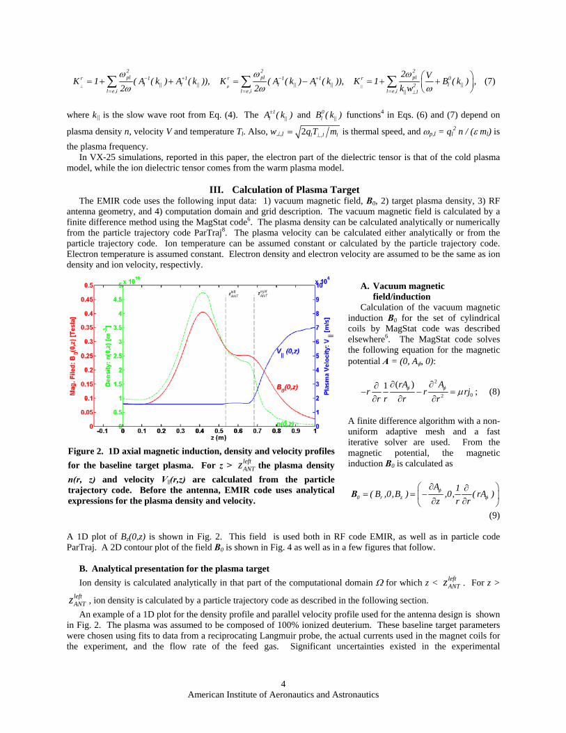
A 1D plot of Bz(0,z) is shown in Fig. 2. This field is used both in RF code EMIR, as well as in particle code ParTraj. A 2D contour plot of the field B0 is shown in Fig. 4 as well as in a few figures that follow.

B. Analytical presentation for the plasma target Ion density is calculated analytically in that part of the computational domain Ω for which z < left

ANTz . For z > leftANTz , ion density is calculated by a particle trajectory code as described in the following section.

An example of a 1D plot for the density profile and parallel velocity profile used for the antenna design is shown in Fig. 2. The plasma was assumed to be composed of 100% ionized deuterium. These baseline target parameters were chosen using fits to data from a reciprocating Langmuir probe, the actual currents used in the magnet coils for the experiment, and the flow rate of the feed gas. Significant uncertainties existed in the experimental

Figure 2. 1D axial magnetic induction, density and velocity profiles for the baseline target plasma. For z > left

ANTz the plasma density n(r, z) and velocity V||(r,z) are calculated from the particle trajectory code. Before the antenna, EMIR code uses analytical expressions for the plasma density and velocity.


measurements of the electron temperature this time, so the flow velocity was chosen as a parameter for study within the reduced order model.

The radial density profile measured at the probe location for the baseline study is shown in Fig. 3. The two-dimensional fit of the baseline density using these parameters is shown in Fig. 4. The density is assumed to be proportional to the magnetic induction strength along the axis, for the case where the ICRF antenna does not accelerate plasma too much. The general two-dimensional dependence of plasma density n(r,z) is reduced to a simpler dependence ni(ψ), where ψ = B0(r,z)r2 is the magnetic flux. There are two options available to define the radial profile of the plasma density. In the “PARABOLIC” option the density is calculated through the following formula

1/ 2 2 4

00 0 0 0

( ) 1n n A B C Dι ι ι ιψ ψ ψ ψψψ ψ ψ ψ

⎛ ⎞⎛ ⎞ ⎛ ⎞⎜ ⎟= + + + +⎜ ⎟ ⎜ ⎟⎜ ⎟⎝ ⎠ ⎝ ⎠⎝ ⎠

(10)

In the “GAUSSIAN” option the density is calculated through the following formula

1/ 2 2 4

00 0 0 0

( ) exp 1n n A B C Dι ι ι ιψ ψ ψ ψψψ ψ ψ ψ

⎛ ⎞⎛ ⎞ ⎛ ⎞⎜ ⎟= + + + +⎜ ⎟ ⎜ ⎟⎜ ⎟⎝ ⎠ ⎝ ⎠⎝ ⎠

. (11)

The ion velocity and temperature fields for z > left

ANTz , are defined by a particle trajectory code as described in

the following section. For z < leftANTz the parallel plasma velocity and temperatures are assumed constant along the

magnetic field lines as shown in Fig. 2.

C. Particle trajectory simulation of the plasma target When plasma is accelerated by the RF power, the density is not proportional to the vacuum magnetic field. It is simulated by a simple version of the particle method, called the “particle trajectory method”, where the plasma fluid characteristics (density, velocity, temperature) are assumed time-independent. Also, collisions are neglected. The ion motion satisfies the following equation of motion with respect to ion position and velocity vectors, xi = (xr, xφ , xz) and vi = (vr, vφ , vz), as functions of time t:

( ( , ) ( , )),i ii i i i i i

d dm q t tdt dt

= × + =v xv B x E x v . (12)

Single particle trajectories are integrated from Eq. (12) with an adaptive time-scheme, which can quickly solve extensive particle simulations for systems of hundreds of thousands of particles in a reasonable time (10 min), and without the need for a powerful supercomputer. The particle calculation method is described in previous publications7,8,9,10. During extensive particle simulation, one needs to define an initial ion velocity distribution, as will be discussed in the following section. Notice, that implementation of the formula (12) requires interpolation of the pre-calculated fields B and E from their grids to the arbitrary position. This is implemented efficiently using a grid-table method.

Figure 3. Radial density profiles were considered based on probe measurements and mapping back along magnetic field lines.


D. Particle to Grid Weighting Here we present our approach of calculating plasma fluid characteristics (density n, velocity V, temperature Ti) based on the kinetic theory, from the calculated particle trajectories, defined by particle positions and velocities (x,and vi). The discrete ion density n is defined constant at each finite difference cell Xj, using the formula

( ) ( )j jk

n w Count= ∈∑ kX x X , (13)

where xk is a position of k-particle, w is a particle weight calculated, such that it makes the grid density equal given value at given point n(X0)=n0: 0

0( )kk

w n Count= ∈∑ x X .

Now, to describe the method of trajectories11. All trajectories start at the same axial position. The choice of that location is made from the following consideration. Only the ICRF area is considered with non-collisional behavior, so that location should be downstream of the flow from the magnet 3, where maximal magnetic strength occurs. Also, it has to be upstream of the flow from the Ion Cyclotron heating location. Thus it can be chosen near left

ANTz . First, the non-uniform grid is generated defining the finite-size cells Xj. Assuming that the vacuum magnetic induction B0 is precomputed on B-grid, as well as RF field Em on RF-grid, allows grid tables to be generated. These grid tables are the fast way to find a grid cell corresponding to the given position xi. With a given distribution for the initial position and velocity vectors at a z near left

ANTz , a large number (order of 105) of ion trajectories are calculated. For simplicity it is assumed that the distribution function at this initial location is a product of radial distribution, velocity magnitude distribution and two velocity slope distributions. Those distributions are chosen such way to satisfy the experimental data, like in Fig. 3. Current simulation assume that a Maxwellian distribution of ion velocity occurs in the flow before it goes into the computational domain inlet at z = left

ANTz . Each single trajectory is used to generate many particles distributed along it with equal time steps between them. Other fluid quantities (velocity V, ion current density j, temperature T and energy W) are calculated by a technique similar to that used to calculate the ion density in (9), as presented below:

( ) : : ( )j k j k j jk k

Count= ∈ = ∈ ∈∑ ∑k k kV X v x X v x X x X , ( ) : i j i k jk

q w= ∈∑ kj X v x X , (14)

2|| ||, ||( ) ( ) : j i k j i j

k kT m v V q Count⎛ ⎞= − ∈ ∈⎜ ⎟

⎝ ⎠∑ ∑k kX x X x X , 2

|| ||,( ) : 2 j i k j i jk k

W m v q Count⎛ ⎞= ∈ ∈⎜ ⎟⎝ ⎠

∑ ∑k kX x X x X .

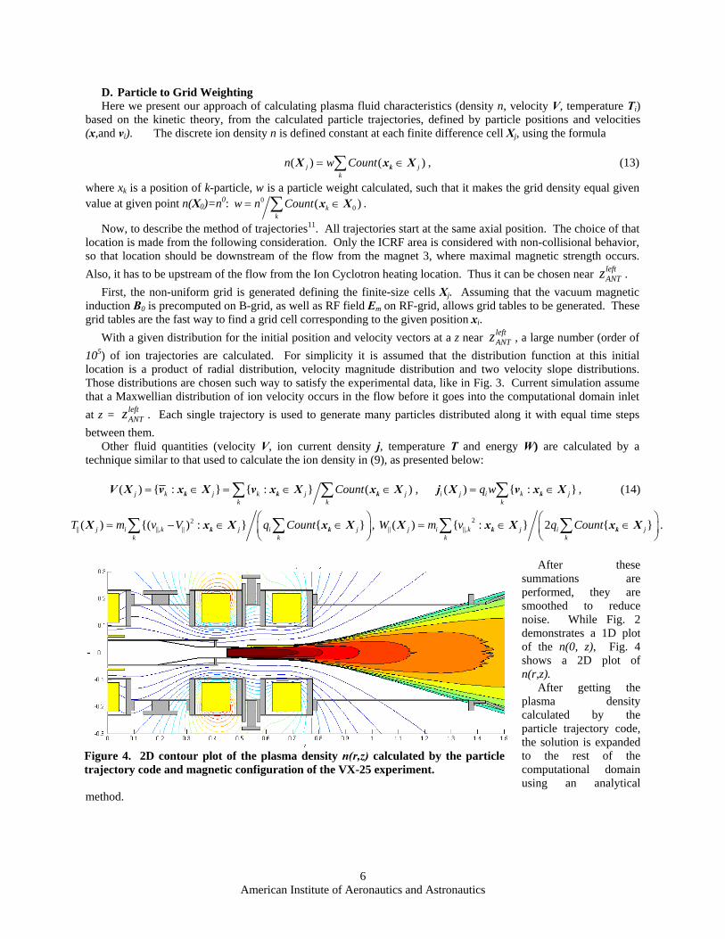
After these summations are performed, they are smoothed to reduce noise. While Fig. 2 demonstrates a 1D plot of the n(0, z), Fig. 4 shows a 2D plot of n(r,z). After getting the plasma density calculated by the particle trajectory code, the solution is expanded to the rest of the computational domain using an analytical

method.

Figure 4. 2D contour plot of the plasma density n(r,z) calculated by the particle trajectory code and magnetic configuration of the VX-25 experiment.


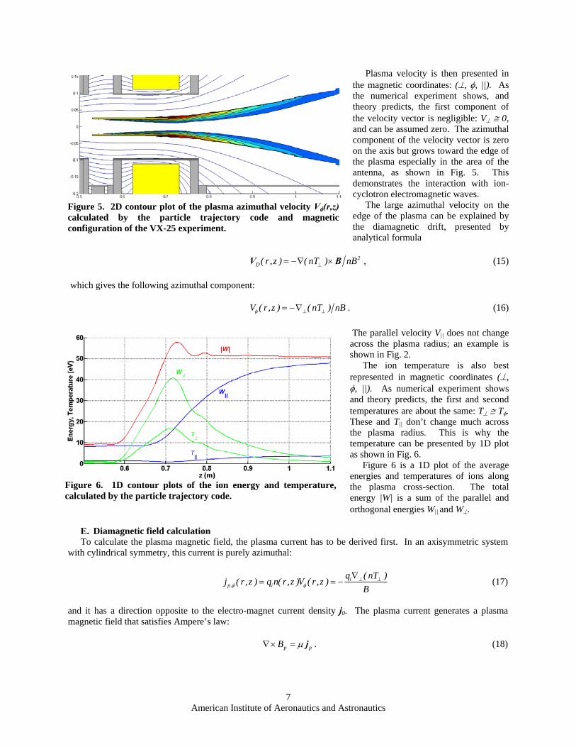
Plasma velocity is then presented in the magnetic coordinates: (⊥, φ, ||). As the numerical experiment shows, and theory predicts, the first component of the velocity vector is negligible: V⊥ ≅ 0, and can be assumed zero. The azimuthal component of the velocity vector is zero on the axis but grows toward the edge of the plasma especially in the area of the antenna, as shown in Fig. 5. This demonstrates the interaction with ion-cyclotron electromagnetic waves. The large azimuthal velocity on the edge of the plasma can be explained by the diamagnetic drift, presented by analytical formula

2

D( r,z ) ( nT ) nB⊥= −∇ ×V B , (15) which gives the following azimuthal component:

V ( r,z ) ( nT ) nBφ ⊥ ⊥= −∇ . (16)

The parallel velocity V|| does not change across the plasma radius; an example is shown in Fig. 2. The ion temperature is also best represented in magnetic coordinates (⊥, φ, ||). As numerical experiment shows and theory predicts, the first and second temperatures are about the same: T⊥ ≅ Tφ. These and T|| don’t change much across the plasma radius. This is why the temperature can be presented by 1D plot as shown in Fig. 6. Figure 6 is a 1D plot of the average energies and temperatures of ions along the plasma cross-section. The total energy |W| is a sum of the parallel and orthogonal energies W|| and W⊥.

E. Diamagnetic field calculation

To calculate the plasma magnetic field, the plasma current has to be derived first. In an axisymmetric system with cylindrical symmetry, this current is purely azimuthal:

ip , i

q ( nT )j ( r,z ) q n( r ,z )V ( r,z )Bφ φ

⊥ ⊥∇= = − (17)

and it has a direction opposite to the electro-magnet current density j0. The plasma current generates a plasma magnetic field that satisfies Ampere’s law:

p pB µ∇× = j . (18)

Figure 5. 2D contour plot of the plasma azimuthal velocity Vφ(r,z) calculated by the particle trajectory code and magnetic configuration of the VX-25 experiment.

Figure 6. 1D contour plots of the ion energy and temperature, calculated by the particle trajectory code.


Figure 7 demonstrates the plasma diamagnetic current and the magnetic field calculated by last equation. The diamagnetic effect is essential only for high magnetic field in the area close to the thruster core and becomes negligible further away from it. The plasma magnetic field is calculated using the same solver, as used for the vacuum magnetic field calculation. The only difference in this calculation is the presence of a current density source jp. Calculation of Bp is iterated with the calculation of plasma velocity and density. For the VX-25 experiment, the maximal diamagnetic field has a strength less than 1% of the vacuum magnetic

field, so the reduction of the total magnetic field is not significant.

IV. RF Power Absorption Simulation The RF power absorbed by the plasma is calculated by the following formula

( )*** m m m mp l l

m l e,i m l e,i

1 1 ˆP Re d Re d Re d p( r,z )d2 2Ω Ω Ω Ω

Ω Ω σ Ω Ω= =

⎡ ⎤ ⎡ ⎤ ⎡ ⎤= ⋅ = ⋅ = ⋅ ⋅ =⎢ ⎥ ⎢ ⎥ ⎢ ⎥

⎣ ⎦ ⎣ ⎦ ⎣ ⎦∑∑ ∑∑∫ ∫ ∫ ∫E j E j E E , (19)

where ( )*m ml

m l e,i

1 ˆp( r,z ) Re2

σ=

⎡ ⎤= ⋅ ⋅⎢ ⎥⎣ ⎦∑∑ E E is a RF power density.

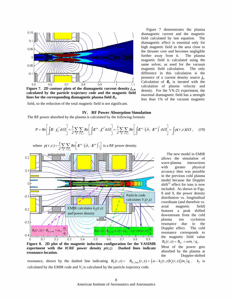
The new model in EMIR allows the simulation of wave-plasma interactions with greater physical accuracy then was possible in the previous cold plasma model because the Doppler shift12 effect for ions is now included. As shown in Figs. 8 and 9, the power density distribution vs. longitudinal coordinate (and therefore vs. axial magnetic field) features a peak shifted downstream from the cold plasma ion cyclotron resonance due to the Doppler effect. The cold resonance corresponds to the magnetic field value

0 ( , ) /IC i iB r z B m qω= = . Most of the power gets absorbed by the plasma at the Doppler-shifted

resonance, shown by the dashed line indicating 0 ( , )B r z = , ( , )IC DopB r z = ( )|| ||( , ) ( , ) i ik r z V r z m qω − . k|| is calculated by the EMIR code and V|| is calculated by the particle trajectory code.

Figure 7. 2D contour plots of the diamagnetic current density jp,φ, calculated by the particle trajectory code and the magnetic field lines for the corresponding diamagnetic plasma field Bp.

( )0 , || ||( , ) ( , ) ( , ) ( , ) iIC Dop IC

i

mB r z B r z k r z V r zq

ω= = −0 ,( , ) iIC cold IC

i

mB r z Bq

ω= =

EMIR calculates k||(r,z)and power density

Particle code calculates V||(r,z)

Figure 8. 2D plot of the magnetic induction configuration for the VASIMR experiment with the ICRF power density p(r,z). Dashed lines indicate resonance location.


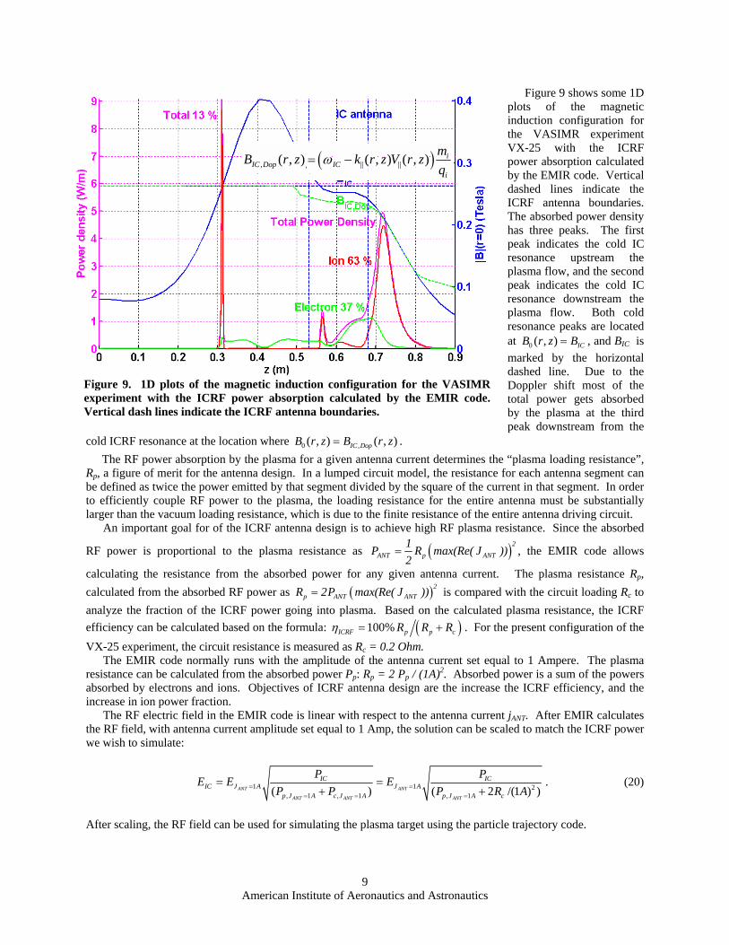
Figure 9 shows some 1D plots of the magnetic induction configuration for the VASIMR experiment VX-25 with the ICRF power absorption calculated by the EMIR code. Vertical dashed lines indicate the ICRF antenna boundaries. The absorbed power density has three peaks. The first peak indicates the cold IC resonance upstream the plasma flow, and the second peak indicates the cold IC resonance downstream the plasma flow. Both cold resonance peaks are located at 0 ( , ) ICB r z B= , and BIC is marked by the horizontal dashed line. Due to the Doppler shift most of the total power gets absorbed by the plasma at the third peak downstream from the

cold ICRF resonance at the location where 0 ,( , ) ( , )IC DopB r z B r z= . The RF power absorption by the plasma for a given antenna current determines the “plasma loading resistance”, Rp, a figure of merit for the antenna design. In a lumped circuit model, the resistance for each antenna segment can be defined as twice the power emitted by that segment divided by the square of the current in that segment. In order to efficiently couple RF power to the plasma, the loading resistance for the entire antenna must be substantially larger than the vacuum loading resistance, which is due to the finite resistance of the entire antenna driving circuit.

An important goal for of the ICRF antenna design is to achieve high RF plasma resistance. Since the absorbed

RF power is proportional to the plasma resistance as ( )2

ANT p ANT1P R max(Re( J ))2

= , the EMIR code allows

calculating the resistance from the absorbed power for any given antenna current. The plasma resistance Rp, calculated from the absorbed RF power as ( )2

p ANT ANTR 2P max(Re( J ))= is compared with the circuit loading Rc to analyze the fraction of the ICRF power going into plasma. Based on the calculated plasma resistance, the ICRF efficiency can be calculated based on the formula: ( )100%ICRF p p cR R Rη = + . For the present configuration of the VX-25 experiment, the circuit resistance is measured as Rc = 0.2 Ohm.

The EMIR code normally runs with the amplitude of the antenna current set equal to 1 Ampere. The plasma resistance can be calculated from the absorbed power Pp: Rp = 2 Pp / (1A)2. Absorbed power is a sum of the powers absorbed by electrons and ions. Objectives of ICRF antenna design are the increase the ICRF efficiency, and the increase in ion power fraction.

The RF electric field in the EMIR code is linear with respect to the antenna current jANT. After EMIR calculates the RF field, with antenna current amplitude set equal to 1 Amp, the solution can be scaled to match the ICRF power we wish to simulate:

1 1 2, 1 , 1 , 1( ) ( 2 /(1 ) )ANT ANT

ANT ANT ANT

IC ICIC J A J A

p J A c J A p J A c

P PE E EP P P R A= =

= = =

= =+ +

. (20)

After scaling, the RF field can be used for simulating the plasma target using the particle trajectory code.

( ), || ||( , ) ( , ) ( , ) iIC Dop IC

i

mB r z k r z V r zq

ω= −

Figure 9. 1D plots of the magnetic induction configuration for the VASIMR experiment with the ICRF power absorption calculated by the EMIR code. Vertical dash lines indicate the ICRF antenna boundaries.


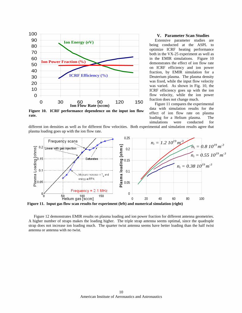
V. Parameter Scan Studies

Extensive parameter studies are being conducted at the ASPL to optimize ICRF heating performance both in the VX-25 experiment as well as in the EMIR simulations. Figure 10 demonstrates the effect of ion flow rate on ICRF efficiency and ion power fraction, by EMIR simulation for a Deuterium plasma. The plasma density was fixed, while the input flow velocity was varied. As shown in Fig. 10, the ICRF efficiency goes up with the ion flow velocity, while the ion power fraction does not change much. Figure 11 compares the experimental data with simulation results for the effect of ion flow rate on plasma loading for a Helium plasma. The simulations were conducted for

different ion densities as well as for different flow velocities. Both experimental and simulation results agree that plasma loading goes up with the ion flow rate.

Figure 12 demonstrates EMIR results on plasma loading and ion power fraction for different antenna geometries. A higher number of straps makes the loading higher. The triple strap antenna seems optimal, since the quadruple strap does not increase ion loading much. The quarter twist antenna seems have better loading than the half twist antenna or antenna with no twist.

0102030405060708090

100

0 30 60 90 120 150Ion Flow Rate (sccm)

ICRF Efficiency (%)

Ion Energy (eV)

Ion Power Fraction (%)

Figure 10. ICRF performance dependence on the input ion flow rate.

0

0.05

0.1

0.15

0.2

0.25

0 20 40 60 80 100

Plas

ma

load

ing

[ohm

s]

ni = 0.38 1019 m-3

ni = 0.55 1019 m-3

ni = 0.8 1019 m-3ni = 1.2 1019 m-3

Figure 11. Input gas flow scan results for experiment (left) and numerical simulation (right)


Figure 13 shows experimental and simulation results for ICRF loading for different magnetic field slopes under the ICRF antenna. Three magnetic field profiles were compared: flat (zero), slightly negative, and slightly positive slopes with the cold ICRF resonance under the middle of the antenna. As both experiment and simulations agree, the best ICRF performance is provided for a magnetic field profile with a slightly positive slope under the antenna. This profile corresponds to the multiple cold ICRF resonance under the antenna. Due to the Doppler shift, all slopes had maximal RF absorption at the area downstream from the antenna.

Figure 12. Analysis of the ICRF plasma loading and the ICRF efficiency as a function of the antenna geometry

+∇B ∇B~0 -∇B

0

0.05

0.1

0.15

0.2

0.25

0.3

0.35

0.9 0.95 1 1.05 1.1 1.15 1.2

experiment

simulation ω/ωci

Figure 13. Analysis of the ICRF plasma resistance as a function of the magnetic field slope under antenna


VI. Conclusions Effective ion cyclotron wave coupling to the plasma has been observed in the VASIMR experiment. Recent plasma parameters considered with the latest ICRF antenna design give a plasma loading with Rp >> Rc, that is, most of the RF transmitter power gets absorbed by the plasma, with more than half directly coupled to the ions. Future design improvements are directed to increase overall VASIMR efficiency by minimizing RF circuit losses, increasing plasma flux from the helicon source and optimizing the magnetic geometry. The EMIR simulation of RF wave propagation in the VASIMR plasma allows us to design the ICRF antenna with improved efficiency, as well as to optimize the magnetic field profile. Recent developments in the EMIR code have resulted in a code performance improvement that will enable further refinement in the physics of the model without sacrificing the fast turnaround of simulation results that is required in the present design effort to support the VASIMR experiment. Future plasma heating simulations in the VASIMR system will involve integration of the EMIR code and particle simulation code into “Numerical VASIMR” simulation software. The plan is to have a self-consistent modeling tool of all significant VASIMR areas: plasma production, plasma booster and exhaust. The next version of the EMIR code will also be parallelizable, and the next version of the particle trajectory code will involve Monte-Carlo collisions.

Acknowledgments This research was supported by NASA Space Operations Mission Directorate (former code M) and the NASA Johnson Space Center. Research and physics development of the EMIR4 code was also provided by Oak Ridge National Laboratory, which is managed by UT-Battelle, LLC, under contract DE-AC05-00OR22725.

References 1 Chang Díaz, F. R., “The VASIMR engine,” Scientific American, Vol. 283, 2000, pp. 72-79. 2 Carter, M. D., Baity, F. W., Barber, G. C., Goulding, R. H., Mori, Y., Sparks, D. O., White, K. F., Jaeger, E. F., Chang Díaz, F.

R. and Squire, J. P. “Comparing Experiments with Modeling for Light Ion Helicon Plasma Sources”, Physics of Plasmas, Vol. 9, 2002, pp. 5097 – 5110.

3 Stix, T. H., Waves in Plasmas, American Institute of Physics, New York, 1992. 4 Ilin, A. V., Chang Díaz, F. R., Squire, J. P., Tarditi, A. G., and Carter, M. D., “Simulation of ICRF Plasma Heating in the

VASIMR Experiment”, Proceedings of 42nd AIAA Aerospace Sciences Meeting and Exhibit’ January 5-8, 2004, Reno, NV, AIAA 2004-0151, 2004, 8 p.

5 Colestock, P. and Kashuba, R. J. “The theory of mode conversion and wave damping near the ion cyclotron frequency”, Nuclear Fusion, Vol. 23, 1983.

6 Ilin, A. V., Chang Díaz, F. R., Gurieva, Y. L. and Il’in, V. P., “Accuracy Improvement in Magnetic Field Modeling for an Axisymmetric Electromagnet”, NASA/TP—2000-210194, 2000, 38 p.

7 Hockney, R. W., and Eastwood, J. W., Computer Simulation Using Particles, Inst. of Physics Publishing, Bristol UK, 1988. 8 Ilin, A. V., Chang Díaz, F. R., Squire, J. P., and Carter, M. D., “Monte Carlo Particle Dynamics in a Variable Specific Impulse

Magnetoplasma Rocket”, Proceedings of Open Systems’ July 27-31, 1998, Novosibirsk, Russia, American Nuclear Society, Trans. of Fusion Tech. Vol. 35, 1999, pp. 330—334.

9 Ilin, A. V., Chang Díaz, F. R., Squire, J. P., Breizman, B. N., and Carter, M. D., “Particle Simulations of Plasma Heating in VASIMR”, Proceedings of 36th AIAA/ASME/SAE/ASEE Joint Propulsion Conference’ July 17-19, 2000, Huntsville, AL, AIAA 2000-3753, 2000, 10 p.

10 Ilin, A. V., Chang Díaz, F. R., Squire, J. P., Tarditi A. G., Breizman, B. N., and Carter, M. D., “Simulations of Plasma Detachment in VASIMR”, Proceedings of 40th AIAA Aerospace Sciences Meeting & Exhibit’ January 14-17, 2002, Reno, NV, AIAA 2002-0346, 2002, 11 p.

11 Ilin, V. P., Numerical Methods for Solving Problems in Electrophysics, (in Russian) Nauka, Moscow, 1985, 335 p. 12 Dendy, R. O., Plasma Dynamics, Clarendon Press, Oxford, 1990, 161 p.

plasma heating simulation in the vasimr system - ad astra … · · 2009-07-29free license to...

Documents