Chapter 7

Plasticity

7.1 Introduction

Various plasticity models of mechanics are developed to describe a class of permanentdeformations. These deformations are generated during loading processes and remainafter the removal of the load. In this Chapter we present a few aspects of the classicallinear plasticity. This model is based on the assumption on the additive separation ofelastic and plastic deformation increments. In nonlinear models it is the deformationgradient F in which these permanent deformations are separated

F = FeFp, (7.1)

where the plastic deformation is described by Fp and the elastic part is Fe. Only theproduct of these two objects is indeed the gradient of the function of motion f . NeitherFe nor Fp can be written in such a form — they are not integrable. In spite of thisproblem, material vectors transformed by Fp form a vector space for each material pointX ∈B0 and these spaces are sometimes called intermediate configurations. We shall notelaborate these issues of nonlinear models1 . However, it should be mentioned that theassumption (7.1) indicates the additive separation of increments of deformation in thelinear model. Namely, the time derivative of the deformation gradient has, obviously,the form

F = FeFp + FeFp, (7.2)

which yields for small strainse = ee + ep, (7.3)

where ee is the elastic strain rate and ep is the plastic strain rate. In some older models itis even assumed that this additive decomposition concerns strains themselves: e = ee+ep

which is obviously much stronger than (7.3) and yields certain general doubts.

1 e.g. see: A�*����� B�����; Elasticity and Plasticity of Large Deformations, Springer Berlin,2008.

135

136 Plasticity

The aim of the elastoplastic models in the displacement formulation is to find thedisplacement vector u whose gradient defines the strain e — as in the case of linearelasticity, and the plastic strain ep which becomes an additional field.

Fig. 7.1: States of material in the stress space Σ. A — the elastic state, B— the plastic state.

The most fundamental characteristic feature of classical plasticity is the distinction ofan elastic domain in the space of stresses Σ = {T} ,T = σijei⊗ ej . All paths of stresseswhich lie in the elastic domain produce solely elastic deformations, i.e. after invertingthe process of loading the material returns to its original state. This is schematicallyshown in Fig. 7.1.

The elastic domain lies within the bounding yield surface also called the yield limit orthe yield locus. Stress states which lie beyond this limit are attainable only by movingthe whole yield surface. Such processes are called hardening. In Fig. 7.1. we demonstratethe so-called isotropic hardening. We return to this notion in the sequel. Increments ofplastic strains are described by stresses whose direction points in the outward directionof the yield surface. This is related to the so-called Drucker2 stability postulate whichwe present further.

The above described way of construction of plasticity is sometimes called stress spaceformulation and it was motivated by properties of metals. There is an alternative whichhas grown up from soil mechanics3 . Such materials as rocks, soils and concrete revealsoftening behaviour which violates Drucker’s postulate. In order to avoid this problem,the so-called strain space formulation4 was developed in which, instead of Drucker’spostulate one applies the Ilyushyn5 postulate. The detailed discussion of these stabilityproblems can be found, for instance, in the book of Wu [24].

2D. C. D� ����; A more fundamental approach to plastic stress-strain relations, in: Proc. 1st Nat.Congress Appl. Mech., ASME, 487, 1951.

3This formulation has been initiated by the work: Z. M�6.; Non-associated flow laws in plasticity,Journ. de Mecanique, 2, 21-42, 1963.

4J. C���4, P. M. N�����; On the nonequivalence of the stress space and strain space formulationsof plasticity theory, J. Appl. Mech., 50, 350, 1983.

5A. A. I�4 ����; On the postulate of plasticity, PMM, 25, 503, 1961.

7.1 Introduction 137

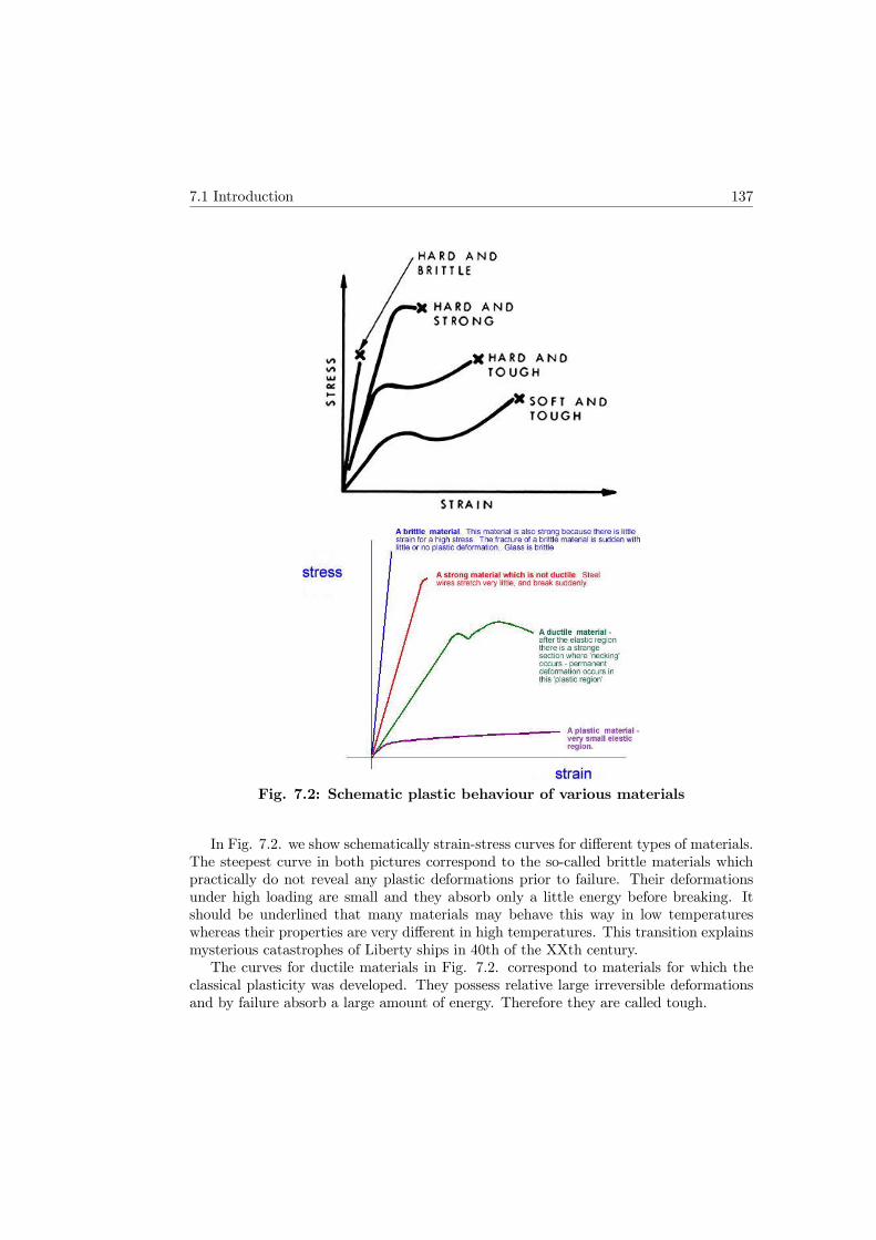
Fig. 7.2: Schematic plastic behaviour of various materials

In Fig. 7.2. we show schematically strain-stress curves for different types of materials.The steepest curve in both pictures correspond to the so-called brittle materials whichpractically do not reveal any plastic deformations prior to failure. Their deformationsunder high loading are small and they absorb only a little energy before breaking. Itshould be underlined that many materials may behave this way in low temperatureswhereas their properties are very different in high temperatures. This transition explainsmysterious catastrophes of Liberty ships in 40th of the XXth century.

The curves for ductile materials in Fig. 7.2. correspond to materials for which theclassical plasticity was developed. They possess relative large irreversible deformationsand by failure absorb a large amount of energy. Therefore they are called tough.

138 Plasticity

Many damages and accidents of cargovessels were occurred, and especiallyfor Liberty Ships. The vast majorityof the sea accidents were relatedto brittle fracture. By 1st of April 1946,1441 cases of damage had been reportedfor 970 cargo vessels, 1031 of which wereto Liberty Ships. Total numbers of 4720damages were reported. Seven ships werebroken in two, e.g. "Schenectady".

7.2 Plasticity of ductile materials

We proceed to specify the yield surface in the stress space. As mentioned above this stressformulation was primarily motivated by plastic deformations of metals. In such materialsthe pressure p has practically no influence on plastic strains which means that the yieldsurface should be described only by the stress deviator: σDij = σij + pδij , p = −13σkk.The eigenvalues of the stress deviator follow from the eigenvalue problem

(σDij − sδij

)nj = 0, (7.4)

and the solutions must satisfy the condition

Is = s(1) + s(2) + s(3) = 0. (7.5)

The eigenvalues s(α) and the eigenvalues σ(α) of the full stress tensor σij are, of course,connected by the relation

σ(α) = s(α) − p, α = 1, 2, 3. (7.6)

For the purpose of formulation of various hypotheses for the yield surface, it is con-venient to calculate invariants of the stress deviator and the maximum shear stresses.As presented in Subsection 3.2.4 (compare the three-dimensional Mohr circles), the ex-tremum values of shear stress are given by the differences of three principal values of thestress tensor (radii of Mohr’s circles)

τ (1) =σ(2) − σ(3)

2, τ (2) =

σ(1) − σ(3)2

, τ (3) =σ(1) − σ(2)

2. (7.7)

Hence, we have as well

τ (1) =s(2) − s(3)

2, τ (2) =

s(1) − s(3)2

, τ (3) =s(1) − s(2)

2. (7.8)

7.2 Plasticity of ductile materials 139

Further we use the sum of squares of these quantities. In terms of invariants of the stresstensor and of the stress deviator it has the form

3∑

α=1

(τ (α)

)2=3

2

[1

3I2σ − IIσ

]= −3

2IIs =

1

2σ2eq, σeq =

√3

2σDijσ

Dij , (7.9)

where σeq = σ(1) in the uniaxial tension/compression for which σ(2) = σ(3) = 0. Itis clear that the second invariant of the deviatoric stresses must be negative. Theserelations follow from the definitions of the invariants

Iσ = σkk = −3p, IIσ =1

2

(I2σ − σijσij

), IIIσ = det (σij) , (7.10)

Is = 0, IIs = −1

2σDijσ

Dij = −J2 = −

σ2eq3, IIIs = J3 = det

(σDij).

The quantity σeq =√3J2 is called the equivalent (effective) stress.

Now, we are in the position to define the elastic domain in the space of stresses. Itis convenient to represent it by a domain in the three-dimensional space of principalstresses. In this space we choose the principal stresses σ(1), σ(2), σ(3) as coordinates. Theassumption that the pressure does not influence plastic strains means that yield surfacesin this space must be cylindrical surfaces with generatrix perpendicular to surfaces s(1)+s(2) + s(3) = 0, i.e. σ(1) + σ(2) + σ(3) + 3p = 0. The axis of those cylinders is, certainly,the straight line σ(1) = σ(2) = σ(3). This line is called the hydrostatic axis. In general,we can write the equation of the yield surface in the form

f(J2, J3, e

pij , κ, T

)= 0, (7.11)

with the parametric dependence on the plastic strain epij , temperature T and the harden-ing parameter κ. We return to these parameters later. Two examples of yield surfaces,discussed further in some details, are shown in Fig. 7.3.

It is also convenient to introduce a normal (perpendicular) vector to the yield surfacein the stress space given by its gradient in this space, i.e.

N =∂f∂T∣∣∣ ∂f∂T∣∣∣, i.e. Nij =

∂f∂σij√∂f∂σkl

∂f∂σkl

. (7.12)

Then we can introduce local coordinates in which the yield function f identifies the elasticdomain of the Σ-space assuming there negative values, i.e. for all elastic processes f < 0.

We skip here the presentation of the history of the definition of yield surfaces whichgoes back to Galileo Galilei. There are two fundamental forms of this surface which arestill commonly used in the linear plasticity of solids. The older one was proposed by H.Tresca in 1864 and it is called Tresca-Guest surface. Its equation has the form

maxα

∣∣∣τ (α)∣∣∣ = σ0 ⇒ σ(1) − σ(3) = 2σ0 > 0, (7.13)

where σ0 is the material parameter and we have ordered the principal stresses σ(1) ≥σ(2) ≥ σ(3). It means that the beginning of the plastic deformation appears in the point of

140 Plasticity

the maximum shear stress. In the space of principal stresses it is a prism of six sides andinfinite length (see: Fig. 7.3.). The parameter σ0 may be dependent on all parameterslisted in the general relation (7.11).

Fig. 7.3: Yield surfaces in the space of principal stresses

The second yield surface was proposed in 1904 by M. T. Huber6 and then rediscoveredin 1913 by R. von Mises and H. von Hencky. It says that the limit of elastic deformationis reached when the energy of shape changes (distortion energy) reaches the limit valueρεY . The distortion energy ρεD is defined as a part of the full energy of deformation ρεreduced by the energy of volume changes ρεV (e.g. compare (5.175)). We have

ρε =1

2σijeij =

1

2

(

σijσkk9K

δij + σijσDij2µ

)

=

=1

2K

(σkk3

)2+1

4µ

(σDijσ

Dij

)⇒ ρεV =

p2

2K, ρεD =

1

4µ

(σDijσ

Dij

), (7.14)

i.e. ρεD = ρεY ⇒ ρεY =1

4µ

(σDijσ

Dij

)=σ2eq6µ

.

Making use of the identity, following from (7.5),

3(s(1)s(2) + s(1)s(3) + s(2)s(3)

)= −1

2

[(s(1) − s(2)

)2+(s(1) − s(2)

)2+(s(1) − s(2)

)2],

(7.15)6M. T. H *��; Przyczynek do podstaw wytrzymałosci, Czasop. Techn., Lwów, 22, 1904. Due to

the publication of this work in Polish it remained unknown until the hypothesis was rediscovered by vonMises and von Hencky.

7.2 Plasticity of ductile materials 141

we obtain

σDijσDij =

1

3

[(s(1) − s(2)

)2+(s(1) − s(2)

)2+(s(1) − s(2)

)2]. (7.16)

Consequently, bearing (7.6) in mind, the yield limit is reached when the principal stressesfulfil the condition

3σDijσDij =

(σ(1) − σ(2)

)2+(σ(2) − σ(3)

)2+(σ(1) − σ(3)

)2= 2σ2Y , (7.17)

i.e. σeq = σY ,

whereσY =

√6µρεY , (7.18)

is the yield limit (σ(1) = σY in uniaxial tension, i.e. for σ(2) = σ(2) = 0). It means thatfor processes in which σeq < σY all states are elastic (f < 0) and otherwise the systemdevelops plastic deformations. Clearly, the relation (7.17) defines a circular cylinder inthe space of principal stresses. Its axis is again identical with the line σ(1) = σ(2) = σ(3),it is extended to infinity and it has common generatrix with the prism of Tresca as shownin Fig. 7.3.⋆In order to compare analytically both definitions of the yield surface we show that

the yield stress σY calculated by means of the distortion energy of the Huber-Mises-Hencky hypothesis (7.17) is not bigger than the material parameter 2σ0 of the Trescahypothesis (7.13). Let us write (7.17) in the following form

σY =1√2

√(σ(1) − σ(2)

)2+(σ(2) − σ(3)

)2+(σ(1) − σ(3)

)2=

=

∣∣σ(1) − σ(3)∣∣

√2

√(σ(1) − σ(2)σ(1) − σ(3)

)2+

(σ(2) − σ(3)σ(1) − σ(3)

)2+ 1 =

=

∣∣σ(1) − σ(3)∣∣

√2

√(1− µσ2

)2+

(1 + µσ2

)2+ 1 =

=∣∣∣σ(1) − σ(3)

∣∣∣

√3 + µ2σ4

, (7.19)

where

µσ =2σ(2) −

(σ(1) + σ(3)

)

σ(1) − σ(3) , (7.20)

is the so-called Lode parameter which describes an influence of the middle principalstress σ(2). Obviously −1 ≤ µσ ≤ 1 which corresponds to σ(2) = σ(3) for the lowerbound, and σ(2) = σ(1) for the upper bound. It plays an important role in the theory ofcivil engineering structures. Hence

σY ≤∣∣∣σ(1) − σ(3)

∣∣∣ = 2σ0.♣ (7.21)

142 Plasticity

⋆ We demonstrate on a simple example an application of the notion of the yieldstress. We consider a circular ring of a constant thickness with external and internalradii a and b, respectively, and an external loading by the pressures pa and pb on thesecircumferences. We check when the material of the ring reaches in all points the yieldstress according to the Huber-Mises-Hencky hypothesis. This is the so-called state of theload-carrying capacity of this structure.

This is the axial symmetric problem of plane stresses. Consequently, the principalstresses in cylindrical coordinates are given by σ(1) = σrr, σ(2) = σθθ, σ(3) = 0. Thesecomponents of stresses must fulfil the equilibrium condition (momentum balance (5.43))

dσrrdr

+σrr − σθθ

r= 0, (7.22)

and, according to (7.17), at each place of the ring

(σrr − σθθ)2 + (σrr)2 + (σθθ)2 = 2σ2Y . (7.23)

By means of (7.22) we eliminate the component σθθ of stresses and obtain the followingequation (

rds

dr

)2+ s

(rds

dr

)+ s2 − 1 = 0, s =

σrr

σY√2. (7.24)

Solution of this quadratic equation with respect to the derivative ds/dr yields

ds

dr= − s

2r± 1

2r

√4− 3s2. (7.25)

Consequentlyds

−s±√4− 3s2

=dr

2r. (7.26)

As we have to require |s| < 2/√3 we can change the variables

s =2√3sinϕ, (7.27)

and this yields

− dϕ

tanϕ∓√3=dr

2r. (7.28)

Hence, we obtain two solutions but only one of them is real and it has the form

r = C

√√√√√√√√

1 +3s2

4− 3s2√s√3

4− 3s2 +√3

exp

[

−√3

2arctan

s√3√

4− 3s2

]

, (7.29)

where C is the constant of integration.

7.2 Plasticity of ductile materials 143

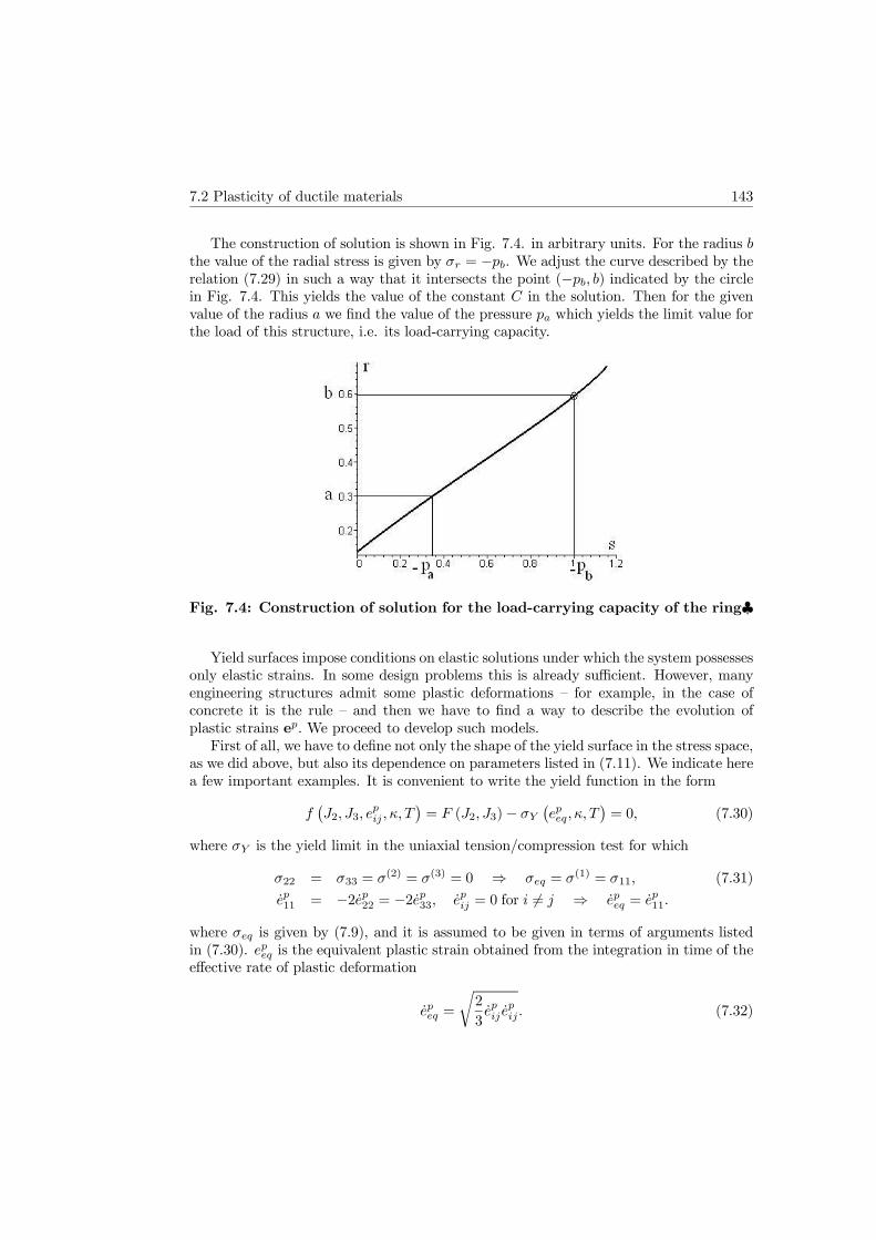
The construction of solution is shown in Fig. 7.4. in arbitrary units. For the radius bthe value of the radial stress is given by σr = −pb. We adjust the curve described by therelation (7.29) in such a way that it intersects the point (−pb, b) indicated by the circlein Fig. 7.4. This yields the value of the constant C in the solution. Then for the givenvalue of the radius a we find the value of the pressure pa which yields the limit value forthe load of this structure, i.e. its load-carrying capacity.

Fig. 7.4: Construction of solution for the load-carrying capacity of the ring♣

Yield surfaces impose conditions on elastic solutions under which the system possessesonly elastic strains. In some design problems this is already sufficient. However, manyengineering structures admit some plastic deformations — for example, in the case ofconcrete it is the rule — and then we have to find a way to describe the evolution ofplastic strains ep. We proceed to develop such models.

First of all, we have to define not only the shape of the yield surface in the stress space,as we did above, but also its dependence on parameters listed in (7.11). We indicate herea few important examples. It is convenient to write the yield function in the form

f(J2, J3, e

pij , κ, T

)= F (J2, J3)− σY

(epeq, κ, T

)= 0, (7.30)

where σY is the yield limit in the uniaxial tension/compression test for which

σ22 = σ33 = σ(2) = σ(3) = 0 ⇒ σeq = σ(1) = σ11, (7.31)

ep11 = −2ep22 = −2ep33, epij = 0 for i �= j ⇒ epeq = ep11.

where σeq is given by (7.9), and it is assumed to be given in terms of arguments listedin (7.30). epeq is the equivalent plastic strain obtained from the integration in time of theeffective rate of plastic deformation

epeq =

√2

3epij e

pij . (7.32)

144 Plasticity

Obviously, for isotropic materials we expect epij to be deviatoric. This yields relations(7.31).

Let us begin with the simplest case. In a particular case of ideal plasticity we considermaterials without hardening. Then the function (7.30) has the form

f =

√3

2σDijσ

Dij − σY = 0, (7.33)

with the constant yield limit σY . Of course, the stress tensor must be such that elasticprocesses remain within the elastic domain which is characterized by f < 0. Plasticdeformations may develop for stresses which belong to the yield surface. Their changesyielding plastic deformation must remain on this surface which means that the incrementsof stresses described by σij must be tangent to the yield surface. Hence, for such processes

f =∂f

∂σijσij = 0, (7.34)

as the gradient ∂f/∂σij is perpendicular to the yield surface.Now we make the fundamental constitutive assumption, specifying the rate of plastic

strain epij and require that this quantity follows from a potential G (σij) defined on thestress space

epij = λ∂G

∂σij, (7.35)

where λ is a scalar function following from the so-called Prager consistency condition.We demonstrate it further.

Let us introduce the notion of the outward normal vector to the surface f = 0 (com-pare (7.12)). Clearly

Nij =∂f

∂σij

∥∥∥∥∂f

∂σkl

∥∥∥∥−1

,

∥∥∥∥∂f

∂σkl

∥∥∥∥ =√

∂f

∂σkl

∂f

∂σkl, (7.36)

is such a vector. For the yield surface (7.33) it becomes

Nij =σDij∥∥σDkl∥∥ ,

∥∥σDkl∥∥ =

√σDklσ

Dkl =

√2

3σY . (7.37)

Obviously, we have the following classification

epij =

{0 for f < 0 or f = 0 and Nijσij < 0.

λ ∂G∂σij

for f = 0 and Nijσij = 0.(7.38)

The condition Nijσij < 0 means that the process yields the unloading — as Nij is or-thogonal to the yield surface, σij must point in the direction of the elastic domain and,consequently, the process must be elastic.

In a particular case when the potential G and the yield function are identical weobtain

7.2 Plasticity of ductile materials 145

epij = λ∂f

∂σij. (7.39)

This is the so-called associated flow rule. In this case, the rate of plastic deformation epijis perpendicular to the yield surface, i.e. it is parallel to the normal vector Nij .

It is appropriate to make here the following remark concerning the geometry of theyield surface. If this surface were not convex then in points in which it is concave tangentchanges of the stress tensor σij , i.e. (∂f/∂σij) σij = 0, would yield stresses in the interiorof the yield surface, i.e. in the range f < 0. This would be related to the developmentof pure elastic deformations in contrast to the assumption that tangent changes of stressyield plastic deformations. Therefore, in the classical plasticity nonconvex yield surfacesare not admissible. This is the subject of the so-called Drucker stability postulate. Inthe local form for the associated flow rules (7.39) it can be written as

epijσij > 0. (7.40)

It is also sometimes postulated in the global form∫ (

σij − σ0ij)depij > 0, (7.41)

which shows that the postulate imposes a restriction on the work of plastic deformationsbetween an arbitrary initial state of stress σ0ij and an arbitrary finite state of stress σij .

For the Huber-Mises-Hencky yield function (7.33) we obtain the associated flow rule

epij = λ

√3

2

σDij∥∥σDkl∥∥ = λ

√3

2Nij . (7.42)

In the simple uniaxial tension/compression test we have then

epeq = ep11 = λ ⇒ epijσij = λ

√3

2

∥∥σDkl∥∥ = λσ11 = epeqσY . (7.43)

Hence for the rate of work (working) we obtain

W = eijσij =(eeij + e

pij

)σij ⇒

⇒ Wp = epijσij = λ

√3

2

∥∥σDkl∥∥ = epeqσeq = epeqσY . (7.44)

The last expression — epeqσY — describes the plastic working in the one-dimensional testwhich is an amount of energy dissipated by the system per unit time due to the plasticdeformation. Hence

λ ≥ 0, (7.45)

and the equality holds only for elastic deformations. This statement follows easily fromthe second law of thermodynamics.

146 Plasticity

In order to construct an equation for plastic strains we account for the additive de-composition (7.3). For f < 0 we have elastic processes and then this property indicates(compare (5.26)) the following Prandl-Reuss equation for the rate of deformation

eij =

(σDij2µ

+σkk9K

δij

)

+ λ

√3

2Nij = (7.46)

=

(σDij2µ

+σkk9K

δij

)

+ Wp

σDij∥∥σDkl∥∥2. (7.47)

This follows from the property of isotropic elastic materials for which the eigenvectorsfor the stress and for the strain are identical7 . The spherical part is, obviously, purelyelastic while the deviatoric part can be written in the form

dσDijdt

+ Wp4µ

3σ2YσDij = 2µ

deDijdt

. (7.48)

This equation is very similar to the evolution equation for stresses within the standardlinear model of viscoelasticity (6.58) divided by the relaxation time τ . However, there isa very essential difference between these two models. It is easy to check that the equationof viscoelasticity (6.58) is not invariant with respect to a change of time scale t → αt,where α is an arbitrary constant. This indicates the rate dependence in the reaction ofthe material. It is not the case for the equation of plasticity (7.48). Differentiation withrespect to time appears in all terms of this equation and for this reason the transformationparameter α cancels out. This is the reason for denoting the consistency parameter byλ = depeq/dt. It transforms: t → αt ⇒ λ → λ/α. Therefore, the classical plasticity israte independent. The response of the system is the same for very fast and very slowtime changes of the loading. In reality, metals do possess this property when the rate ofdeformation epeq is approximately 10−6−10−4 1/s. For higher rates one has to incorporatethe rate dependence (compare the book of Lemaitre, Chaboche [9] for further details).This yields viscoplastic models presented further in these notes.

In the more general case of isotropic hardening and for isothermal processes σY be-comes a function of epeq alone. For many materials it is also important to include thetemperature dependence. Then σY becomes the function of these two quantities. Themodel is similar to this which we have considered above but one has to correct the defin-ition of the consistency parameter λ. Finally, a dependence on the hardening parameterκ means that we account for the accumulation of plastic deformations in the material.The most common definitions of this parameter are as follows

a) the parameter accounting for the accumulation of the plastic energy

κ =

t∫

0

σij (ξ) epij (ξ) dξ, (7.49)

7 In order to prove it, it is sufficient to compare the eigenvalue problems for deviatoric stress andstrain tensors.

7.2 Plasticity of ductile materials 147

b) Odqvist parameter accounting for the accumulation of the plastic deformation(compare (7.30) and (7.32))

κ =

t∫

0

√2

3epij e

pijdξ =

t∫

0

depeqdξ

dξ. (7.50)

Then the relation (7.11) yields the consistency condition

f = 0 ⇒ ∂f

∂σijσij +

∂f

∂epijepij +

∂f

∂TT +

∂f

∂κκ = 0. (7.51)

Simultaneously, epij �= 0 only in processes of loading which are defined by the relation

∂f

∂σijσij +

∂f

∂TT > 0. (7.52)

In the limit case∂f

∂σijσij +

∂f

∂TT = 0, (7.53)

we say that the process is neutral. Finally, for the process of unloading,

∂f

∂σijσij +

∂f

∂TT < 0. (7.54)

Consequently, for the evolution of plastic deformation we have the following relations

epij =

0 for either f < 0 or f = 0 and ∂f∂σij

σij +∂f∂T T ≤ 0

λ∂f

∂σijfor f = 0 and ∂f

∂σijσij +

∂f∂T T > 0.

(7.55)

In the case of the hardening parameter (7.49) the consistency condition (7.51) can bewritten in the form

f =∂f

∂σklσkl +

∂f

∂TT +

[∂f

∂epij++

∂f

∂κσij

]

epij = 0.

Hence, we obtain the following relation for the consistency parameter

λ =

∂f∂σkl

σkl +∂f∂T T

D, D = − ∂f

∂epij

∂f

∂σij− ∂f

∂κ

∂f

∂σijσij . (7.56)

The quantity D is called the hardening function. We have

λ > 0 ⇒ D > 0. (7.57)

The flow rule can be now written in the form

epij =1

D

∂f

∂σij

(∂f

∂σklσkl +

∂f

∂TT

). (7.58)

148 Plasticity

The right hand side is the homogeneous function of σij and T . Consequently, this flowrule possesses the same time invariance as the rule (7.39) for the model without hardening,i.e. the model is rate independent.

Apart from the above presented isotropic hardening materials reveal changes of theyield limit which can be attributed to the shift of the origin in the space of stresses. Atypical example is the growth of the yield stress in tensile loading with the simultaneousdecay of the yield stress for compression. In the uniaxial case it means that the wholestress-strain diagram will be shifted on a certain value of stresses. This is the Bauschingereffect.

Fig. 7.5: An example of Bauschinger effect in cyclic loading

The corresponding hardening is called kinematical or anisotropic. It is described bythe so-called back-stress Z = Zijei⊗ej which specifies the shift of the origin in the stressspace. The yield function can be then written in the form

f (T,Z, κ) = F (T,Z)− σY(epeq, T

)=

√3

2σDij σ

Dij − σY = 0, (7.59)

whereσDij = σDij − Zij . (7.60)

One has to specify an equation for the back-stress. It is usually assumed to have theform of the evolution equation, e.g.

Zij = β (σij − Zij) , (7.61)

where β is a material parameter. We skip here the further details referring to numerousmonographs on the subject8 .

8 e.g. see the book [9] orA�*����� B�����; Elasticity and Plasticity of Large Deformations, Springer Berlin, 2008.M����7 K���*��; Handbook of Computational Solid Mechanics, Springer, Heidelberg, 1998.G����� A. M� ���; The Thermomechanics of Plasticity and Fracture, Cambridge University Press,

1992.

7.3 Plasticity of soils 149

7.3 Plasticity of soils

Theories of irrecoverable, permanent deformations of soils is very different from theplasticity of metals presented above. Metals produce plastic deformations primarilydue to the redistribution and production of crystallographic defects called dislocations.Plastic behaviour of soils is mainly connected with the redistribution of grains and it isstrongly influenced by fluids filling the voids (pores) of such a granular material. Straindue to the deformation of grains is often negligible in comparison to the amount of shearand dilatation caused by relative motions of grains. The behaviour is entirely differentin the case of dry granular materials (frictional materials) than a material saturated by,for instance, water or oil where the cohesive forces play an important role. A detailedmodern presentation of the problem of permanent deformations of soils can be found inthe book of D. Muir Wood [23] (compare also a set of lectures von Verruijt [19]). Similarissues for rocks are presented in the classical book of Jaeger, Cook and Zimmerman[6].We limit the attention only to few issues of this subject.

Attempts to describe the plasticity of granular materials stem from Coulomb, whoformulated a simple relation between the normal stress σn on the surface with a normalvector n and the shear stress τn on this surface. It is a generalization of the law offriction between two bodies and has the form

|τn| = c− σn tanϕ, (7.62)

where ϕ is the so-called friction angle (angle of repose) and c denotes the cohesionintercept. This relation is called Mohr-Coulomb law. For dry granular materials thecohesion does not appear, c = 0, and then the angle of repose ϕ is the only materialparameter. It is, for instance, the slope of natural sand hills and pits (Fig. 7.6).

Fig. 7.6: Sand pit trapof antlion in dry sand.Slope almost equal to ϕ

The above relation leads immediately to the yield function in terms of principalstresses σ(1) > σ(2) > σ(3).. Namely

f(σ(1), σ(2), σ(3)

)=(σ(1) − σ(3)

)+(σ(1) + σ(3)

)sinϕ− 2c cosϕ = 0. (7.63)

150 Plasticity

The derivation from properties of Mohr’s circle is shown in Fig. 7.7. Namely

|τn| =σ(1) − σ(3)

2cosϕ, σn =

σ(1) + σ(3)

2− σ(1) − σ(3)

2sinϕ. (7.64)

Substitution in (7.62) yields (7.63).For ϕ = 0 and c = σ0 the yield function (7.63) becomes the Tresca-Guest yield

condition (7.13).

Fig. 7.7: Construction of Mohr-Coulomb yield function

Cohesive forces are influencing not only the relation between normal and shear stresses.Due to the porosity of granular materials a fluid in pores yields cohesive interactions aswell as it carries a part of external loading. This observation was a main contribution ofvon Terzaghi to the theory of consolidation of soils9 . He has made an assumption thatthe pore pressure p does not have an influence on the plastic deformation of soils. Themeaning of p is here the same as in Subsection 6.4. and it should not be confused withthe trace of the bulk stress σij , i.e. p �= −13σkk. It means that the stress appearing inyield functions must be reduced by subtracting the contribution of this pressure. If wedefine the effective stress

σ′ij = σij + pδij , (7.65)

then the Mohr-Coulomb yield function becomes(σ′(1) − σ′(3)

)+(σ′(1) + σ′(3)

)sinϕ− 2c cosϕ = 0. (7.66)

σ′(α) = σ(α) + p, α = 1, 2, 3.

This function is shown in the upper panel of Fig. 7.8.Further we distinguish by primes all quantities based on the effective stress.

9K. '�� T��.����; Erdbaumechanik auf bodenphysikalischer Grundlage, Franz Deuticke, Wien, 1925.

7.3 Plasticity of soils 151

Incidentally, a similar notion of effective stresses appears in the theory of damage — itis related to changes of reference surface due to the appearance of cracks. Such modelsshall be not presented in these notes.⋆Remark. There exists some confusion within the soil mechanics concerning the

definition of positive stresses. Soils carry almost without exception only compressiveloads (compare Fig. 7.7. and 7.8.) and, for this reason, in contrast to the classicalcontinuum mechanics, a compressive stress is assumed to be positive. This is convenientin a fixed system of coordinates related to experimental setups such as triaxial apparatus.Then pressure p in the definition of effective stresses (7.65) would appear with the minussign. Usually it is denoted in soil mechanics by u. In some textbooks10 both conventionsconcerning the sign of stresses appear simultaneously. However, such a change of signin a general stress tensor yields the lack of proper invariance with respect to changes ofreference systems. It is also contradictory with the choice of the positive direction ofvectors normal to material surfaces on which many mathematical problems of balancelaws and the Cauchy Theorem rely. For these reasons, we work here with the sameconvention as in the rest of this book — tensile stress is positive.

In addition, one should be careful in the case of relation of such one-component modelsto models following from the theory of immiscible mixtures, for instance to Biot’s model.Such models are based on partial quantities and then the pore pressure p is not the partialpressure pF of a multicomponent model but rather p = pF/n, where n is the porosity.♣

In soil mechanics, where the definitions of elastic domains described in the previousSubsection are not appropriate, it is convenient to introduce special systems of referencein the space of effective principal stresses. One of them is directly related to the set ofinvariants (7.10)

p′ =1

3I ′1 = −

1

3I ′σ, q =

√3J ′2 = σeq, r = 3

3

√J ′32. (7.67)

Another one is a cylindrical system. One of the axes is the pressure(−13σ′kk

), i.e. it

is oriented along the line σ′(1) = σ′(2) = σ′(3). It is denoted by ξ and scaled ξ = I ′σ/√3.

The other two coordinates are defined by the relations

ρ =√2J ′2 ≡

√2

3σ′eq ≡

√σ′Dij σ

′Dij , cos (3θ) =

(r

σ′eq

)3. (7.68)

These are the so-called Haigh—Westergaard coordinates. The (ξ, ρ)- planes are calledRendulic planes and the angle θ is called the Lode angle. The transformation from thesecoordinates back to principal stresses is given by the relation

σ′(1)

σ′(2)

σ′(3)

=1√3

ξξξ

+√2

3ρ

cos θ

cos(θ − 2

3π)

cos(θ + 2

3π)

. (7.69)

Mohr-Coulomb yield function in the Haigh—Westergaard coordinates has the followingform [√

3 sin(θ +

π

3

)− sinϕ cos

(θ +

π

3

)]ρ−√2ξ sinϕ =

√6c cosϕ. (7.70)

10 e.g. [23] or R. L����������; Geotechnical Engineering, Balkema, Rotterdam, 1995.

152 Plasticity

Alternatively, in terms of the invariants (p′, q, r) we can write[

1√3 cosϕ

sin(θ +

π

3

)− 13tanϕ cos

(θ +

π

3

)]q − p′ tanϕ = c, (7.71)

θ =1

3arccos

(r

q

)3.

As in the classical theory of plasticity, modifications of Mohr-Coulomb condition wereintroduced in order to eliminate corners in the yield surface. One of such modificationswas introduced by D. C. Drucker and W. Prager. This condition for the limit state ofsoils has the following form

√J ′2 −

√3 cosϕ

√3 + sin2 ϕ

c− sinϕ√3(3 + sin2 ϕ

)I′σ = 0, (7.72)

where the invariants J ′2 and I ′σ are defined by relations for effective stress analogousto (7.10). This function is shown in the lower panel of Fig. 7.8. The dependence onthe invariant I ′σ follows from the dependence of the yield in soils on volume changes,i.e. it describes an influence of dilatancy on the appearance of the critical limit state.For ϕ = 0 and c = σY /

√3 this condition becomes identical with Huber-Mises-Hencky

condition (7.17).Due to its simplicity the Mohr-Coulomb yield surface is often used to model the

plastic flow of geomaterials (and other cohesive-frictional materials). However, manysuch materials show dilatational behavior under triaxial states of stress which the Mohr-Coulomb model does not include. Also, since the yield surface has corners, it maybe inconvenient to use the original Mohr-Coulomb model to determine the direction ofplastic flow. Therefore it is common to use a non-associated plastic flow potential thatis smooth. For example, one is using the function

g =

√(αcY tanψ)

2+G2 (ϕ, θ) q2 − p′ tanϕ, (7.73)

where α is a parameter, cY is the value of c when the plastic strain is zero (also calledthe initial cohesion yield stress), ψ is the angle made by the yield surface in the Rendulicplane at high values of p′ (this angle is also called the dilation angle), and G (ϕ, θ) is anappropriate function that is also smooth in the deviatoric stress plane.

7.3 Plasticity of soils 153

Fig. 7.8: Yield surfaces (7.66) and (7.72) in the space of principal effectivestresses σ1 = σ′(1), σ2 = σ′(2), σ3 = σ′(3).

We shall not expand this subject anymore. Due to the vast field of applications: soils,powders, avalanches, debris flows and many others, the number of models describing thecritical behaviour of such materials is also very large. Cap plasticity models, Cam-Clay(CC) models, Modified-Cam-Clay (MCC) models, Mroz models, etc. are based on similarideas as the models presented above. There exists also a class of hypoplasticity modelsin which the notion of the yield surface does not appear at all and which seem to fit wellphenomena appearing in sands11 .

11 compare articles of E. B� ��: Analysis of Shear Banding with a Hypoplastic Constitutive Modelfor a Dry and Cohesionless Granular Material, 335-350, and D. K��4*��: The Importance of Sandin Earth Sciences, both in: B. A�*��� (ed.); Continuous Media with Microstructure, Springer, Berlin,2010.

154 Plasticity

7.4 Viscoplasticity

There are many ways of extension of the classical plasticity to include rate dependence.Obviously, one of them would be to incorporate additionally some viscous propertiesas we did in Chapter 7. This kind of the model is developed since early works of P.Perzyna12 . The other way, less ambitous, is to incorporate a rate dependence in thedefinition of the yield function. In principle, the classical yield function cannot exist insuch models but one gets results by direct extension of plasticity models presented inthis Chapter. For such models it is advocated in the books of Lemaitre, Chaboche [9]and Lemaitre, Desmorat [10].

We present here only a few hints to the model of the second kind. Namely, it isassumed that the yield criterion satisfies the relation

f = 0, f = 0 — plasticity,

f = σV > 0 — viscoplasticity, (7.74)

with f < 0 satisfied in the elastic domain. σV is a viscous stress given by a viscosity law.In both cases f can be chosen according to the rules discussed in previous Subsections.For instance, in the case of Huber-Mises-Hencky model with isotropic and kinematichardening we have

f = (T−Z)eq − κ− σY , (7.75)

(T−Z)eq =

√3

2

(σDij − ZD

ij

) (σDij − ZD

ij

),

where κ describes the isotropic hardening related to the size growth of the yield surface.It may be, for instance, assumed to have the exponential form

κ = κ∞[1− exp

(−bepeq

)], (7.76)

where κ∞, b are material parameters depending on temperature. Sometimes a power lawκ = Kp

(epeq)1/M

is sufficient.Kinematic hardening described by the back-stresses Zij requires an evolution equa-

tion. It may have the form (7.61) or it may be the so-called Armstrong-Frederick law13

d

dt

(ZijC

)=2

3epij −

γ

CZij e

peq, (7.77)

for which the identification of parameters is easier [10].The viscous stress σV is also given by various empirical relations. Two of them have

the form1) Norton power law

σV = KN

(epeq)1/N

, (7.78)

12 e.g. P. P��.4��; The constitutive equations for the rate sensitive plastic materials, Quart. Appl.Math., 20, 321-332, 1963.

13P. J. A�������, C. O. F��������; A mathematical representation of the multiaxial Bauschingereffect, CEGB Report, RD/B/N731, Berkeley Nuclear Laboratories, 1966.

7.4 Viscoplasticity 155

2) exponential law leading to the saturation at large plastic rates

σV = K∞

[1− exp

(−epeqn

)], (7.79)

where KN ,K∞, N and n are material parameters.In Fig. 7.9 we show a comparison of results for various viscous models14 .

Fig. 7.9: Relaxation test for the identification of viscosity parameters —Inconel alloy at θ = 6270 C.

For the alloy investigated by Lemaitre and Dufailly the following parameters areappropriate

E = 160 GPa, KN = 75 GPa/s1/N , N = 2.4, K∞ = 104 GPa, n = 1.4× 10−2s−1.

Rate-dependent viscoplastic models must be used in cases of high deformation rates.For metals, the rates up to app. 10−3 1/s do not influence substantially results in theplastic range of deformations. For higher rates the yield limit may grow even three timesby the rate 100 1/s15 .

14J. L������, J. D -����4; Damage measurements, Engn. Fracture Mech., 28, 1987

15P. P��.4��; Thermodynamics of Inelastic Materials (in Polish), PWN, Warsaw, 1978.

156 Plasticity