please scroll down for article - ubc …nancy/papers/gijbels_heckman.pdf · a ‘burn-in’ process...

PLEASE SCROLL DOWN FOR ARTICLE

This article was downloaded by: [Canadian Research Knowledge Network]On: 6 August 2008Access details: Access Details: [subscription number 783016891]Publisher Taylor & FrancisInforma Ltd Registered in England and Wales Registered Number: 1072954 Registered office: Mortimer House,37-41 Mortimer Street, London W1T 3JH, UK

Journal of Nonparametric StatisticsPublication details, including instructions for authors and subscription information:http://www.informaworld.com/smpp/title~content=t713645758

Nonparametric testing for a monotone hazard function via normalized spacingsIrène Gijbels a; Nancy Heckman b

a Institute of Statistics, Catholic University of Louvain, Louvain-la-Neuve, Belgium b Department of Statistics,The University of British Columbia, Vancouver, BC, Canada

Online Publication Date: 01 June 2004

To cite this Article Gijbels, Irène and Heckman, Nancy(2004)'Nonparametric testing for a monotone hazard function via normalizedspacings',Journal of Nonparametric Statistics,16:3,463 — 477

To link to this Article: DOI: 10.1080/10485250310001622668

URL: http://dx.doi.org/10.1080/10485250310001622668

Full terms and conditions of use: http://www.informaworld.com/terms-and-conditions-of-access.pdf

This article may be used for research, teaching and private study purposes. Any substantial orsystematic reproduction, re-distribution, re-selling, loan or sub-licensing, systematic supply ordistribution in any form to anyone is expressly forbidden.

The publisher does not give any warranty express or implied or make any representation that the contentswill be complete or accurate or up to date. The accuracy of any instructions, formulae and drug dosesshould be independently verified with primary sources. The publisher shall not be liable for any loss,actions, claims, proceedings, demand or costs or damages whatsoever or howsoever caused arising directlyor indirectly in connection with or arising out of the use of this material.

http://www.informaworld.com/smpp/title~content=t713645758

http://dx.doi.org/10.1080/10485250310001622668

http://www.informaworld.com/terms-and-conditions-of-access.pdf

Nonparametric StatisticsVol. 16(3–4), June–August 2004, pp. 463–477

NONPARAMETRIC TESTING FOR A MONOTONEHAZARD FUNCTION VIA NORMALIZED SPACINGS

IRENE GIJBELSa,∗ and NANCY HECKMANb,†

aInstitute of Statistics, Catholic University of Louvain, Voie du Roman Pays 20, B-1348Louvain-la-Neuve, Belgium; bDepartment of Statistics, The University of British Columbia,

Vancouver BC, V6T 1Z2, Canada

(Received 22 January 2003; Revised 15 July 2003; In final form 30 July 2003)

We study the problem of testing whether a hazard function is monotonic or not. The proposed test statistics, a globaltest and four localized tests, are all based on normalized spacings. The global test is in fact just the test statistic[Proschan, F. and Pyke, R. (1967). Tests for monotone failure rate. Fifth Berkeley Symposium, 3, 293–313], introducedfor testing a constant hazard function versus a nondecreasing nonconstant hazard function. This global test is powerfulfor detecting global departures of the null hypothesis, but lacks power when there are local departures from the nullhypothesis. By localizing the global test, we obtain tests that respond to this drawback. We also show how the testingprocedures can be used when dealing with Type II censored data. We evaluate the performance of the test statisticsvia simulation studies and illustrate them on some data sets.

Keywords: Monotone hazard function; Order statistics; Spacings; Type II censoring

1 INTRODUCTION

The distribution of a variable of interest is commonly characterized via the cumulativedistribution function, the probability density function, or the characteristic function. Whendealing with ‘lifetimes’ though it is often more useful to describe the distribution via the hazardfunction, which is the instantaneous risk of ‘dying’ given ‘survival’ up to the present time.Owing to their interpretation, hazard functions are a handy tool for modeling. For example, theinstantaneous risk of ‘dying’ might be higher in one group than another. Therefore, the studyof lifetimes is often done via the hazard function. When talking about ‘lifetime’, we areautomatically thinking of a positive random variable. The word ‘lifetime’ is used here in abroad sense: it denotes the time of the occurence of a certain specified event. Examples ofevents are ample: death of an individual or the appearance of a tumor in a medical study,failure of a machine in a factory or the ‘breaking down’ of a product in a quality-controlexperiment in engineering.

Hazard functions can have various shapes. The most important ones are: monotoneincreasing hazards, bathtub-shaped or U-shaped hazards, monotone decreasing hazards. Thehuman lifetime can be appropriately described by a bathtub-shaped hazard: there is an initial

∗ E-mail: [email protected]† Corresponding author. E-mail: [email protected]

ISSN 1048-5252 print; ISSN 1029-0311 online c© 2004 Taylor & Francis LtdDOI: 10.1080/10485250310001622668

Downloaded By: [Canadian Research Knowledge Network] At: 23:53 6 August 2008

464 I. GIJBELS AND N. HECKMAN

period with high risk due to birth defects or infant diseases, followed by a period of moreor less constant risk; after a while the risk starts increasing again due to the aging process.Models with increasing hazard are frequently used. For example, manufacturers often usea ‘burn-in’ process for their products: the products are subjected to operation before beingsold to customers. In this way, an initial early failure of defective items is prevented and theitems that are put on the market exhibit gradual aging. Decreasing hazards can be useful whenmodeling survival time after a successful medical treatment. More examples of typical hazardfunctions are provided in Lawless (1982). See this reference for inference procedures for themost important parametric models also.

There are early references on nonparametric estimation of a hazard function with kernelestimators for the hazard function (Watson and Leadbetter, 1964a, b), and with estimation ofthe cumulative hazard function (Nelson, 1969). The literature on nonparametric estimationof a hazard function under monotonicity constraints is rather limited. Maximum likelihoodestimators for an increasing hazard function were studied in Grenander (1956), Marshall andProschan (1965), Padgett and Wei (1980), Myktyn and Santner (1981), Wang (1986), Tsai(1988), Mukerjee and Wang (1993) and Huang and Wellner (1995). Recently, Hall et al. (2001)proposed a method for monotonizing kernel-type estimators of a hazard function. The methodis based on a ‘biased bootstrap’ (Hall and Presnell, 1999).

In this paper, we study the problem of testing

H0: the hazard function is nonincreasing versus

H1: the hazard function increases on some interval. (1)

Our methods can also be applied to testing

H0: the hazard function is nondecreasing versus

H1: the hazard function decreases on some interval. (2)

If we reject the hypothesis of monotonicity, then we should not consider modeling survivaltimes via a certain parametric family, such as the Weibull, which always has a monotonehazard. On the other hand, if we can accept the hypothesis that the hazard is monotone, wemay more accurately estimate it by using an appropriate parametric family or by a constrainednonparametric estimate. Furthermore, confirming or disproving monotonocity is of interestin its own right: if we believe that the hazard function of time to relapse after a treatment isdecreasing, then we know that the positive effect of the treatment increases over the time spanconsidered.

Most papers in the literature focus on testing the null hypothesis of a constant hazard rateversus the alternative of a nondecreasing, nonconstant hazard rate:

H R0 : the hazard function is constant versus

H R1 : the hazard function is a nondecreasing, nonconstant function. (3)

This is a rather restricted testing problem. The null hypothesis is equivalent to testing thatlifetimes are exponentially distributed and the alternative hypothesis only involves a rathersmall class of nonconstant functions.

In many situations observations are censored, that is we do not observe the particular eventdefining the lifetime. For example, an individual might drop out of a medical study beforethe actual end of the study and hence one only knows that his lifetime is larger than theobserved time. Censoring complicates but does not preclude inference on the distribution ofthe survival times.


TESTING FOR A MONOTONE HAZARD 465

In the uncensored case, seminal work on testing H R0 versus H R

1 has been done in Proschanand Pyke (1967), Bickel and Doksum (1969) and Bickel (1969). These tests are based onnormalized spacings, which we define in Eq. (6). These tests were extended in Barlow andProschan (1969) to handle Type I censored data. Other tests for the complete data case werealso proposed (Barlow and Doksum, 1972; Ahmad, 1975; Klefsjo, 1983), among others. Forrandomly censored data, Gerlach introduced a test statistic based on a measure of the deviationof the lifetime distribution from a lifetime distribution with increasing failure rate (Gerlach,1987). This was generalized, with a proposal of a general class of statistics using weightfunctions (Kumazawa, 1992). Related references on goodness-of-fit testing for exponentialityare given in Gail and Gastwirth (1978a, b), among others. Recently, Hall et al. (2001) presenteda nonparametric test based on evaluating the distance between the monotonized estimator andthe standard kernel estimator. This test depends on the smoothing parameter involved in thekernel estimator. Another testing procedure, less dependent on smoothing parameter selection,is introduced in Hall and Van Keilegom (2002).

Our testing procedures are localized versions of the test of Eq. (3) as in Proschan and Pyke(1967), a test based on comparisons of all normalized spacings. We show in Section 3 thatthis test can also be used for testing the null hypotheses (1) and (2). While the test is powerfulfor the alternative hypothesis of a monotone hazard, it is not designed to test against the moregeneral alternative hypotheses of (1) and (2). Our local versions of their test do not focus onan overall comparison of spacings, but rather are based on comparisons belonging to certain‘local’ regions. Our ideas are inspired by recent developments in nonparametric testing usinglocal techniques (Gijbels et al., 2000; Hall and Heckman, 2000). The advantage of our tests incomparison to the recently proposed nonparametric test in Hall et al. (2001) and Hall and VanKeilegom (2002) is that our tests do not depend on a smoothing parameter. Dumbgen (2002)gives another approach to localized data analysis, wherein the main goal is to identify timeintervals where the hazard is likely to be increasing or decreasing.

Based on simulation studies, we find that our local tests of (1) are more powerful than theglobal test when the true hazard is decreasing except on a small interval, where it is increasing.When the hazard is increasing except for a small interval of decrease, the local methods arecomparable to or slightly better than the global test. When the hazard is strictly increasing, theglobal test is most powerful, as expected.

The paper is organized as follows. In Section 2, we briefly describe some preliminary factsabout hazard functions that will be necessary for a clear explanation of the testing procedures.These procedures are introduced in Section 3, and evaluated via a simulation study in Section 4.In the same section, we also illustrate our procedures on a real data set. In Section 5, we describeanalysis of Type II censored data and apply our methodology to a data set. Some conclusionsand further discussion are provided in Section 6.

2 DECREASING AND INCREASING HAZARD FUNCTIONS

Let T be the nonnegative variable of interest, and denote by F the distribution function ofT . Assume for a moment that T is a continuous random variable with density f . The hazardfunction of T is then defined for values of t with F(t) < 1 as

h(t) = lim�→0+

pr{t ≤ T < t + �|T ≥ t}�

.

Thus h(t) represents the risk that an individual or item fails immediately after time t givensurvival up to time t . The cumulative hazard function is defined via the survival function



S(t) = 1 − F(t) = pr{T > t}:H (t) = − log S(t),

but can also be defined as H (t) = ∫ t0 h(u) du. The hazard function then equals h(t) =

−d{log S(t)}/dt = f (t)/{1 − F(t)}. Similar definitions of the hazard function and thecumulative hazard function can be given in the case of a discrete random variable T or inthe case of a mixed discrete–continuous random variable. Our method is valid in general, forany nonnegative random variable T .

We first recall a simple fact about the hazard and the cumulative hazard function, which willallow us to formulate testing problems that are equivalent to problems (1) and (2) but whichdo not require T to have a density. Proposition 1 states that the monotonicity of the hazardfunction h(·) can be formulated in terms of the convexity/concavity of the cumulative hazardfunction H (·). A proof of this proposition can be found in Barlow and Proschan (1965).

PROPOSITION 1 The following statements are equivalent:

(i) h(t) is a nondecreasing (respectively nonincreasing) function(ii) H (t) is a convex (respectively concave) function on {t ≥ 0: F(t) < 1} ≡ [0, τF [,

where τF denotes the upper endpoint of the support of F, i.e. τF = sup{t ≥ 0: F(t) < 1}.

As a consequence of this proposition, testing problem (1) is equivalent to

H0: H is a concave function on [0, τF [ versus

H1: H is not a concave function,(4)

and testing problem (2) is equivalent to

H0: H is a convex function on [0, τF [ versus

H1: H is not a convex function.(5)

We will focus on testing problem (1) or (4) since this will allow us to stay close to the originaldescription of the test in Proschan and Pyke (1967). In Remark 2 in Section 3, we will indicatehow to use our test procedures for testing (2) or equivalently (5).

We now briefly describe the test in Proschan and Pyke (1967), proposed for testing (3),and justify later on that it can be used for testing the null hypothesis in (1). Note first that thenull hypothesis H R

0 is equivalent to H R0 : T has an exponential distribution. See for example

Lawless (1982). The null hypothesis in (1) describes a much larger class of functions, includingthe case of the exponential distribution.

Let T1, . . . , Tn be a sample of independent and identically distributed random variablesfrom T , and denote by 0 ≡ T(0) ≤ T(1) ≤ T(2) ≤ · · · ≤ T(n) the order statistics of the observedtimes. The test in Proschan and Pyke (1967) is based on the normalized spacings

Dni = (n − i + 1)(T(i) − T(i−1)), i = 1, . . . , n, (6)

and uses the test statistic

Vn =n∑

i, j=1,i< j

Vi j with Vi j = I {Dni > Dn j}. (7)

The null hypothesis is rejected when the observed value of Vn is too large. Our tests will alsobe based on the normalized spacings, but will not compare all of them in a global sense as isdone in Eq. (7). We will be more selective in comparing the normalized spacings and workmore locally.



To understand this test statistic one needs to have insights into the behavior of the normali-zed spacings, which have been studied in detail in the literature. See for example Barlow andProschan (1965),Appendix 2, and earlier references provided therein, as well as Robertson et al.(1988). Some known facts about the normalized spacings are summarized in Proposition 2.Recall that a random variable U is said to be stochastically smaller (larger) than a randomvariable W if pr{U > u} ≤ pr{W > u} for all u (respectively pr{U > u} ≥ pr{W > u} forall u). We use the notation U ≤st W (U ≥st W ) for indicating that U is stochastically smaller(larger) than W . The proof of item (i) below can be found in Epstein and Sobel (1953), whereasan easily accessible proof of items (ii) and (iii) is given in Robertson et al. (1988).

PROPOSITION 2

(i) If the Ti s are exponentially distributed with mean θ then Dn1, . . . , Dnn are independentexponential random variables with mean θ .

(ii) If the Ti s have a nonincreasing hazard function then Dn1 ≤st Dn2 ≤st · · · ≤st Dnn.

(iii) If the Ti s have a nondecreasing hazard function then Dn1 ≥st Dn2 ≥st · · · ≥st Dnn .

An immediate consequence of Proposition 2(i) is that, for i, j = 1, . . . , n, i �= j, the Vi j sare Bernoulli distributed with pr{Vi j = 1} = 1/2 if the Ti s are exponentially distributed. FromProposition 2(ii) and (iii), we might suspect that, for i < j , pr{Vi j = 1} is less than 1/2 if theTi s have a decreasing hazard function and is greater than 1/2 if the Ti s have an increasinghazard function. This is indeed the case, as shown in Proschan and Pyke (1967) and implied byparts (ii) and (iii) of the theorem in the following section. Motivated by these facts Proschanand Pyke (1967) proposed rejecting H R

0 in favor of H R1 when Vn is too big. Determining the

critical region for this test is straightforward in principle since the distribution of the Vi j s isdetermined under the null hypothesis H R

0 of exponentiality.

3 TEST STATISTICS

We now consider several testing procedures for testing problem (1). All of our test statistics arenondecreasing functions of the Vi j s, i < j . We prove below that we can calculate the signifi-cance levels of our tests using rejection probabilities calculated for exponentially distributedlifetimes. We also argue heuristically that our tests will have some power against the alternativehypothesis. To accomplish this we first transform the lifetimes to exponential random variablesand then compare the Vi js from the original lifetimes to the Vi j s of the transformed lifetimes.Specifically let

T 0i = H (Ti) = − log S(Ti ), i = 1, . . . , n, (8)

and let V 0i j be the indicator variable, defined similarly as Vi j but based on the T 0

i s. The proof ofthe following theorem is similar to that in Proschan and Pyke (1967), but is given here briefly,for clarity.

THEOREM

(i) The random variables T 01 , . . . , T 0

n are independent and identically distributed having anexponential distribution with unit mean.

(ii) If H is concave on an interval [a, b[, then V 0i j ≥ Vi j for i < j, i, j = 1, . . . , n, if T(i−1)

and T( j) are in the interval [a, b[.(iii) If H is convex on an interval [a, b[, then V 0

i j ≤ Vi j for i < j, i, j,= 1, . . . , n, if T(i−1)

and T( j) are in the interval [a, b[.



Remark 1 When testing whether the hazard function is decreasing on the whole domain, weconsider [a, b[ equal to [0, τF [. See Proposition 1. If, on the other hand, we want to test whetherthe hazard function is decreasing on a certain subset of its domain then we will choose theinterval [a, b[ accordingly.

Proof of the Theorem Proof of statement (i). The random variables T 01 , . . . , T 0

n are indepen-dent since T1, . . . , Tn are independent. Moreover, it is easy to show that Ti is exponentiallydistributed with unit mean.

Proof of statement (ii). If H is concave on [a, b[, then this implies that for all i < j

H (T(i)) − H (T(i−1))

T(i) − T(i−1)

≥ H (T( j)) − H (T( j−1))

T( j) − T( j−1)

whenever T(i−1) and T( j) are in [a, b[. Since H is a nondecreasing function, the ordering of theT 0

i s is the same as that of the Ti s. Let T 0(1) ≤ T 0

(2) ≤ · · · ≤ T 0(n) be the ordered T 0

i s. Thus

T 0(i) − T 0

(i−1)

T 0( j) − T 0

( j−1)

≥ T(i) − T(i−1)

T( j) − T( j−1)

or alsoD0

ni

D0n j

≥ Dni

Dn j.

Consequently, if Vi j = 1, then V 0i j = 1. If Vi j = 0, then V 0

i j can equal 0 or 1. Hence, in general,V 0

i j ≥ Vi j , for all i < j .Proof of statement (iii). This is similar to the proof of statement (ii) but relies on the convexity

of H . �

The following Corollary follows immediately.

COROLLARY Let T1, . . . , Tn be independent and identically distributed survival times, T 0i as

defined in (8), let V be a nondecreasing function of the Vi j s, i < j , with Vi j as defined in (6)and (7), and let V 0 be the corresponding statistic based on the T 0

i s.

(i) If H is concave on an interval [a, b[, and all the Ti s fall in this interval, then V 0 ≥ V .(ii) If H is convex on an interval [a, b[, and all the Ti s fall in this interval, then V 0 ≤ V .

Suppose that, in the testing problem (1), we reject H0 when V > c, where V satisfies theconditions of the Corollary. We now easily see that the significance level α can be calculatedassuming lifetimes have an exponential distribution. Indeed, for all nonincreasing hazard func-tions h or, equivalently, all concave cumulative hazard functions H , we find from Corollary (i)that pr{V > c} ≤ pr{V 0 > c}, for all c, and since a constant hazard is just an element of thisclass of nonincreasing hazard functions, we have

α = suph nonincreasing

pr{V > c} = pr{V 0 > c}.

Thus, to calculate the critical region of the test or the p-value we simulate samples of indepen-dent and identically distributed random variables from an exponential distribution with unitmean, and calculate the statistic V 0.



Corollary (ii) gives us an heuristic indication that our test might have power if the hazardis increasing on some interval [a, b[: we would expect our test statistic V to be large becauseof that interval of increase.

Remark 2 It is easy to see that our generic test statistic V can also be used for testingproblem (2). Indeed, from part (iii) of the Theorem, we see that, for H convex and i > j,V 0

i j ≥ Vi j . So it suffices to work with the original test statistic V but with the reverse of thenormalized spacings, DI

ni ≡ Dn,n−i+1.We consider five tests, all of which are based on test statistics which are nondecreasing

functions of the Vi j s for i < j , and we reject the null hypothesis when the test statistic is large.Our first statistic is Vn , as proposed in Proschan and Pyke (1967), which we call the globalsign test, denoted by

Tglobal ≡ Vn =n∑

i, j=1,i< j

Vi j . (9)

The other four test statistics are localized versions of Tglobal.A first local version is obtained by summing not all indicator variables, but using a local

sum and taking the maximum over these local sums. More precisely, for two indices s and k,with values in the set {1, . . . , n} and such that s + k ≤ n, define the local sum

Vsk =∑

s≤i< j≤s+k

Vi j .

Note that Tglobal = V1,n−1. We see that Vsk measures the monotonicity of the hazard in theinterval (T(s−1), T(s+k)), since Vi j depends on T(i−1), T(i), T( j−1), and T( j). Before taking amaximum over s and k, we normalize Vsk to take account of the number of terms in the sum.The mean and variance of the statistic Tglobal under H R

0 (i.e. exponentiality of the Ti s) are inProschan and Pyke (1967): E(Tglobal) = n(n − 1)/4 and var (Tglobal) = (2n + 5)(n − 1)n/72.This result was obtained in Mann (1945). The mean and variance of the quantity Vsk are easilyobtained from these expressions by taking n = k + 1. So, if the Tis are exponentially distributedwe have

µk ≡ E(Vsk) = (k + 1)k

4vk ≡ var(Vsk) = (2k + 7)(k + 1)k

72.

Let V∗sk denote the normalized local sums: V∗

sk = v−1/2k (Vsk − µk). Then the local sign test is

defined as

Tlocal = max1≤s≤n−1

max1≤k≤n−s

V∗sk . (10)

Our other three tests use comparisons of spacings that are separated by a certain index, sayk with k ≥ 1. The three tests differ in the way we normalize Vsk(r)s and in the values of s, kand r used when taking the maximum. More precisely, define

Vsk(r) =r∑

i=0

Vs+i,s+i+k .

We see that Vsk(r) measures monotonicity in the interval (T(s−1), T(s+r+k)). The differencebetween Vsk and Vsk(r) is that the former studies monotonicity via Dni , Dnj with i and jboth close together and far apart, while Vsk(r) restricts attention to j − i = k. For a strictlyincreasing hazard one Dni is more likely to be greater than Dnj when j − i is large. Thus one



might anticipate that a test based on Vsk(r) has more power than a test based on Vsk . However,our final test statistics involve taking the maximum over k, in order to detect departures frommonotonicity in small intervals. So the power benefit of these ‘skip’ tests is unclear. Oursimulation study indicates that two of the ‘skip’ tests might have higher power than Tlocal.

For one test, we use the fact that, if the Ti s are independent and exponentially distributedrandom variables, and hence the normalized spacings Dni s are independent and identicallydistributed exponential random variables, then

µ(r) ≡ E{Vsk(r)} = r + 1

2vk(r) ≡ var{Vsk(r)} = r + 1

4− (r + 1 − k)+

6,

where y+ = max(y, 0). The calculation of µ(r) is straightforward since Vsk(r) is a sum of(possibly) dependent Bernoulli random variables with success probabilities 1/2. The calcu-lation of Vk(r) involves the calculation of covariances among Vi j s and careful counting ofsimilar terms. Let V∗

sk(r) denote the normalized quantity:V∗sk = vk(r)−1/2{Vsk(r) − µ(r)}. We

then define the test statistic

Tskip = max1≤s≤n−1

max1≤k≤n−s

max0≤r≤n−k−s

V∗sk(r), (11)

which we call the local skip test since it skips spacings.Another statistic is obtained by approximating the variance ofVsk(r) assuming that all terms

in the sum are independent Bernoulli random variables with success probability 1/2. We thusobtain the approximated variance

v(r) = r + 1

4.

The local skip test using this approximated variance will be based on V∗sk(r) = v(r)−1/2

{Vsk(r) − µ(r)}, and leads to the test statistic

Tskip approx = max1≤s≤n−1

max1≤k≤n−s

max0≤r≤n−k−s

V∗sk(r), (12)

which we will call the approximate local skip test.Our last test statistic only considers Vsk(r) with r ≤ k − 1. Note that, in this case and

assuming exponentially distributed lifetimes, Vsk(r) is indeed a sum of independent Bernoullidistributed random variables. Also, v(r) = vk(r). Our restricted local skip test is defined as

Tskip rest = max1≤s≤n−1

max1≤k≤n−s

max0≤r≤min(k+1,n−k−s)

V∗sk(r). (13)

4 ANALYSIS WITH UNCENSORED DATA

4.1 Simulation Study

In this section, we evaluate the performance of the five tests discussed in Section 3 for testingproblem (1) via a simulation study.

In our simulations, we model the logarithm of the hazard function as

log h(t) = a0 + a1 log t + β(2πσ 2)−1/2 exp

{− (t − µ)2

2σ 2

}. (14)



The first two terms are the logarithm of the Weibull hazard, and are obviously increasing(decreasing) when a1 is positive (negative). For β sufficiently large, the third term induces abump at location t = µ and so the hazard is not monotone.

When a1 = β = 0, (14) is the exponential log hazard. Figures 1 and 2 illustrate propertiesof the model for several values of parameters: a0 = 0, µ = 1, a1 = −0.2 or 0.1, β = 0 or 0.3,σ = 0.1 or 0.2. Figure 1 shows the densities, the hazards and the cumulative hazards, the firstand last calculated numerically. Figure 2 shows plots of the 5th, 25th, 50th, 75th and 95thpercentiles of the normalized spacings Dni as a function of i , for the case that n = 50. Thesepercentiles were calculated via 1000 simulated data sets. In general, when a1 is positive thehazard has an overall increasing trend and the normalized spacings have a decreasing trend.When a1 is negative the opposite holds. The trend is more pronounced for large values of |a1|.Decreasing σ or increasing β produces a sharp peak in the hazard function or equivalently adip in the normalized spacings.

FIGURE 1 Densities (top row), hazards (middle row) and cumulative hazards (bottom row) for the log hazard (14)with a0 = 0 and µ = 1. The plots on the left side are with a1 = −0.2 and the plots on the right side are with a1 = 0.1.In each plot, the three curves correspond to β = 0 (dashed), β = 0.3 and σ = 0.2 (dotted), and β = 0.3 and σ = 0.1(solid).



FIGURE 2 Plots of the pointwise quantiles (5th, 25th, 50th, 75th, 95th) of the normalized spacings Dni versus ifor n = 50. Data were generated using log hazard (14) with a0 = 0 and µ = 1. In the left column, we have takena1 = −0.2 and the right column a1 = 0.1. In the first row, β = 0, so the lifetimes follow a Weibull distribution. Inthe second row β = 0.3 and σ = 0.2, and in the third row β = 0.3 and σ = 0.1.

For each parameter configuration considered, we generated 1000 data sets of size 50 andcalculated our five test statistics. Table I contains the proportion of times out of 1000 thatH0 is rejected at the 0.05 level. The standard errors of these proportions are approximately0.01. Our 0.05 rejection rule is determined using the results of Section 3, that p-values canbe calculated assuming that the 50 lifetimes are exponentially distributed. We calculated ourp-values using a ‘null distribution’ table based on 2000 simulated exponential data sets. InTable I, the only configurations of parameters that are contained within the null hypothesisare β = 0 with a1 = −0.2,−0.1 or 0.0. Of the local statistics, the restricted local skip testin (13) and the approximate local skip test in (12) are almost never less powerful than the localskip test in (11) and the local sign test in (10), and are usually significantly more powerful.Note that the performances of the restricted local skip test and the approximate local skip testare almost identical. Indeed, closer inspection of the simulation study shows that these twostatistics agree about 80% of the time, because the maximum value of the normalized Vsk(r)soccurs when r ≤ k + 1. The global sign test in (9) is powerful when the overall trend of thehazard is increasing (a1 > 0), but its performance relative to the local tests deteriorates as wemove further from the Weibull. For values of a1 ≤ 0 and β �= 0, we see that the global signtest is less powerful than the local tests. Thus the local tests are better than the global sign testat detecting the bump in a decreasing log hazard. The differences between the global test andthe local tests increase as the value of |a1| increases.

Our simulation results actually hold for a family of parameters, by the following argument.The Vi j s, and hence our statistics, are scale invariant, that is they are not changed if the lifetimesare multiplied by a positive constant. Thus our simulations for lifetimes with survival functionS(·) hold for data with survival function S∗(·) = S(·/γ ), γ > 0. Translating this condition into



TABLE I Proportion of Times the Null Hypothesis Is Rejected at the 5%Level for Survival Times with Log Hazard (14).

a1

−0.2 −0.1 0.0 0.01

β = 0Global 0.001 0.017 0.05 0.189Skip rest 0.010 0.025 0.05 0.095Skip approx 0.012 0.022 0.05 0.092Skip 0.034 0.043 0.05 0.087Local 0.029 0.043 0.05 0.089

β = 0.3, σ = 0.2Global 0.014 0.055 0.128 0.289Skip rest 0.066 0.118 0.184 0.267Skip approx 0.078 0.123 0.180 0.247Skip 0.061 0.101 0.143 0.184Local 0.063 0.087 0.142 0.190

β = 0.3, σ = 0.1Global 0.024 0.102 0.229 0.410Skip rest 0.139 0.255 0.336 0.478Skip approx 0.143 0.269 0.338 0.478Skip 0.118 0.197 0.240 0.373Local 0.147 0.219 0.301 0.393

conditions on the hazard function, we see that our results for parameter values a0, a1, β, σ, µ

also hold for parameter values a∗0 = a0 − (a1 + 1) log γ, a∗

1 = a1, β∗ = γβ, σ ∗ = γ σ and

µ∗ = γµ.We also conducted a simulation study to compare our testing methods to the simulation

results in Hall et al. (2001). That paper considers the testing problem (2), with data simulatedfrom a model with hazard h(t) = αβ(αt)β−1 exp{−(αt)β} with α = 1.5 and β = 0.4(0.1)1.1.

We consider sample size n = 50 and tests of level 0.05. When β = 0.4, the hazard functionis decreasing, so we should easily reject H0. In Hall et al. (2001) H0 is rejected 91.75% ofthe time, and our local methods are comparable with, for example, the restricted local skipmethod rejecting 94.5% of the time. As expected for decreasing hazards, the global methodis very powerful, rejecting 99.5% of the time. When β = 1.0 or 1.1, the hazard function isincreasing and therefore we should not reject the null hypothesis. Here, our tests outperformthe test in Hall et al. (2001). The global test never rejects H0, the restricted local skip test andthe approximate local skip test reject less than 1% of the time, and our other two tests reject1 or 2% of the time. In contrast, the test in Hall et al. (2001) rejects 6.5% or 5.25% of thetime. When β = 0.5, . . . , 0.9 the hazard function is bathtub shaped. All methods lose poweras β increases, but our methods lose power more rapidly than in Hall et al. (2001). In fact,when β = 0.9, our methods perform poorly, rejecting less than 3% of the time, compared torejection rate of 8% as described in Hall et al. (2001). However, when β = 0.9, the bathtub-shaped hazard is mainly decreasing and the normalized spacings are mainly increasing. Whenwe try our methods to test the null hypothesis that the hazard function is nondecreasing wefind that the global test rejects the null hypothesis 55.5% of the time and the restricted localskip test rejects 31% of the time.

4.2 Illustration with Real Data

We now study the hazard function for the lifetime of ball bearings. The data set, originallydiscussed in Lieblein and Zelen (1956), can be found in Lawless (1982, p. 228), and consists



FIGURE 3 The bearings data. The left plot contains the estimate of the cumulative hazard. The right plot is of thenormalized spacings Dni versus i .

of the number of revolutions (in millions) before failure of 23 ball bearings. In Lieblein andZelen (1956), the data are analyzed with a Weibull model, and in Lawless (1982) with theWeibull and the log normal model, which has a hazard that increases then decreases.

Figure 3 contains a plot of the estimated cumulative hazard, calculated as the negative ofthe logarithm of 1 minus the empirical distribution function. The plot on the right side of thefigure gives the normalized spacings Dni versus i . From Figure 3, we see that the cumulativehazard might be convex and that the normalized spacings have an overall decreasing trend. Wefirst test (1) and then test (2) as described in Remark 2 of Section 3. The p-values are presentedin Table II. Both the global and local sign tests reject the hypothesis that the cumulative hazardis concave. All tests give very high p-values for testing the null hypothesis that the cumulativehazard is convex. We conclude that the cumulative hazard function is not concave but maybe convex.

TABLE II The p-Values for Testing the Ball Bearings Data.

(1): H0: nonincreasing hazard (2): H0: nondecreasing hazard

Global 0.008 0.990Skip rest 0.130 0.643Skip approx 0.182 0.722Skip 0.114 0.920Local 0.000 0.601



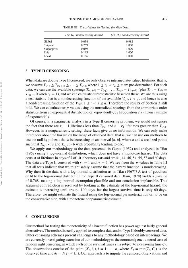
TABLE III The p-Values for Testing the Mice Data.

(1): H0: nonincreasing hazard (2): H0: nondecreasing hazard

Global 0.034 0.982Skiprest 0.259 1.000Skipapprox 0.089 1.000Skip 0.193 1.000Local 0.186 1.000

5 TYPE II CENSORING

When data are double Type II censored, we only observe intermediate-valued lifetimes, that is,we observe T(r1) ≤ T(r1+1) ≤ · · · ≤ T(r2), where 1 ≤ r1 < r2 ≤ n are pre-determined. For suchdata, we can use the available spacings T(r1+1) − T(r1), . . . , T(r2) − T(r2−1) (plus T(1) − T(0) ≡T(1) − 0 when r1 = 1), and we can calculate our test statistic based on these. We are thus usinga test statistic that is a nondecreasing function of the available Vi js, i < j , and hence is alsoa nondecreasing function of the Vi j s, 1 ≤ i < j ≤ n. Therefore the results of Section 3 stillhold. We can calculate our p-values using the normalized spacings from the appropriate orderstatistics from an exponential distribution or, equivalently, by Proposition 2(i ), from a sampleof exponentials.

Of course, in a parametric analysis in a Type II censoring problem, we would not ignorethe fact that there are r1 − 1 lifetimes less than T(r1) and n − r2 lifetimes greater than T(r2).However, in a nonparametric setting, these facts give us no information. We can only makeinferences about the hazard on the range of observed data, that is, we can use our methods totest the null hypothesis that h is decreasing on an interval [a, b[, where a and b are fixed pointssuch that T(r1) < a and T(r2) > b with probability tending to one.

We apply our methodology to the data presented in Gupta (1952) and analyzed in Tiku(1967) using a log–normal distribution, which does not have a monotone hazard. The dataconsist of lifetimes in days of 7 of 10 laboratory rats and are 41, 44, 46, 54, 55, 58 and 60 days.The data are Type II censored with r1 = 1 and r2 = 7. We see from the p-values in Table IIIthat all tests indicate that we might safely assume that the hazard function is nondecreasing.Why then fit the data with a log–normal distribution as in Tiku (1967)? A test of goodnessof fit to the log–normal distribution for Type II censored data (Bain, 1978) yields a p-valueof 0.768, making a log–normal assumption plausible and our conclusion implausible. Thisapparent contradiction is resolved by looking at the estimate of the log–normal hazard: theestimate is increasing until around 100 days, but the largest survival time is only 60 days.Therefore, we might estimate the hazard using the log–normal parameterization or, to be onthe conservative side, with a monotone nonparametric estimate.

6 CONCLUSIONS

Our method for testing the monotonicity of a hazard function has power against fairly generalalternatives. The method is easily applied to complete data and to Type II doubly censored data.Other censoring schemes present challenges to any methodology based on interspacings. Weare currently investigating extension of our methodology to the commonly encountered case ofrandom right censoring, in which each of the survival times Ti is subject to a censoring time Ci .The observations consist of the pairs (Xi , δi), i = 1, . . . , n, where Xi = min(Ti , Ci ) is theobserved time and δi = I {Ti ≤ Ci }. Our approach is to impute the censored observations and



then use the ‘completed’ data set to calculate normalized spacings and then our test statistics.Various reasonable methods of imputation are possible. However, a method for calculatingp-values by a Monte Carlo procedure is not obvious and requires investigation. Clearly wecannot ignore the fact that the original data were censored and that we have imputed values inorder to calculate a test statistic. Therefore we must be able to incorporate censoring into ourMonte Carlo scheme, most likely via an estimate of the censoring time distribution.

The paper of Hall and Van Keilegom (2002) contains a different test of the monotonicity ofthe hazard function and introduces a different method for calculating the p-value. The authorscalculate p-values using a smoothed data-based distribution, roughly speaking, the distributionin the null hypothesis that is closest to the observed data. We calculate p-values by taking thesupremum over the null hypothesis of the probability of rejection. The test in Hall and VanKeilegom (2002) may be more powerful than ours, but it is not clear if the size of the test ismaintained under the exponential distribution. This method of calculating the p-value warrantsfurther exploration, and may improve the power of our testing procedure.

Acknowledgements

This research was supported by ‘Projet d’Actions de Recherche Concertees’, No. 98/03-217 of the Belgian government, by IAP research network no. P5/24 of the Belgian State(Federal Office for Scientific, Technical and Cultural Affairs) and by the Natural Sciences andEngineering Research Council of Canada. The second author would like to thank the Instituteof Pure and Applied Mathematics and the Institute of Statistics of the Universite Catholiquede Louvain, for the financial support and their hospitality. Both authors thank Michael Akritasand an anonymous referee for their careful reading of the paper.

References

Ahmad, I. A. (1975). A nonparametric test for the monotonicity of a failure rate function. Commun. Stat. A-Theor.,A4, 967–974.

Bain, L. J. (1978). Statistical Analysis of Reliability and Life-testing Models: Theory and Methods. M. Dekker, NewYork.

Barlow, R. E. and Doksum, K. (1972). Isotonic tests for convex orderings. Proceedings of the Sixth Berkeley Symposium,1, 293–323.

Barlow, R. E. and Proschan, F. (1965). Mathematical Theory of Reliability, The SIAM series in Applied Mathematics.John Wiley, New York.

Barlow, R. E. and Proschan, F. (1969). A note on tests for monotone failure rate based on incomplete data. Ann. Math.Stat., 40, 595–600.

Bickel, P. J. (1969). Tests for monotone failure rate II. Ann. Math. Stat., 40, 1250–1260.Bickel, P. J. and Doksum, K. A. (1969). Tests for monotone failure rate based on normalized spacings. Ann. Math.

Stat., 40, 1216–1235.Dumbgen, L. (2002). Application of local rank tests to nonparametric regression. J. Nonparametr. Stat., 14, 511–537.Epstein, B. and Sobel, M. (1953). Life testing. J. Am. Stat. Assoc., 48, 486–502.Gail, M. H. and Gastwirth, J. L. (1978a). A scale-free goodness-of-fit test for the exponential distribution based on

the Lorentz curve. J. Am. Stat. Assoc., 73, 787–793.Gail, M. H. and Gastwirth, J. L. (1978b). A scale-free goodness-of-fit test for the exponential distribution based on

the Gini statistic. J. Roy. Stat. Soc. B, 40, 350–357.Gerlach, B. (1987). Testing exponentiality against increasing failure rate with randomly censored data. Statistics, 18,

275–268.Gijbels, I., Hall, P., Jones, M. C. and Koch, I. (2000). Tests for monotonicity of a regression mean with guaranteed

level. Biometrika, 87, 663–673.Grenander, U. (1956). On the theory of mortality measurement, Part II. Skand. Akt. 39, 125–153.Gupta, A. K. (1952). Estimation of the mean and standard deviation of a normal population from a censored sample.

Biometrika, 39, 260–273.Hall, P. and Heckman, N. (2000). Testing for monotonicity of a regression mean by calibrating for linear functions.

Ann. Stat., 28, 20–39.Hall, P., Huang, L.-S., Gifford, J. and Gijbels, I. (2001). Nonparametric estimation of hazard rate under the constraint

of monotonicity. J. Comput. Graph. Stat., 10, 592–614.



Hall, P. and Presnell, B. (1999). Intentionally biased bootstrap methods. J. Roy. Stat. Soc. B, 61, 259–277.Hall, P. and Van Keilegom, I. (2002). Testing for monotone increasing hazard rate, manuscript.Huang, J. and Wellner, J. (1995). Estimation of a monotone density or monotone hazard under random censoring.

Scand. J. Stat., 22, 3–33.Klefsjo, B. (1983). Some tests against aging based on the total time on test transform. Commun. Stat. A-Theor., A12,

907–927.Kumazawa, Y. (1992). Tests for increasing failure rate with randomly censored data. Statistics, 23, 17–25.Lawless, J. F. (1982). Statistical Models and Methods for Lifetime Data. Wiley, New York.Lieblein, J. and Zelen, M. (1956). Statistical investigation of fatigue life of deep groove ball bearings. J. Res. Nat. Bur.

Stand., 57, 273–316.Mann, H. B. (1945). Nonparametric tests against trend. Econometrica, 13, 245–259.Marshall, A. W. and Proschan, F. (1965). Maximum likelihood estimation for distributions with monotone failure rate.

Ann. Math. Stat., 36, 69–77.Mukerjee, H. and Wang, J.-L. (1993). Nonparametric maximum likelihood estimation of an increasing hazard rate for

uncertain cause-of-death data. Scand. J. Stat., 20, 17–33.Myktyn, S. and Santner, T. (1981). Maximum likelihood estimation of the survival function based on censored data

under hazard rate assumptions. Communications in Statistics–Theory & Methods, A10, 1369–1387.Nelson, W. B. (1969). Hazard plotting for incomplete failure data. J. Qual. Technol. 1, 27–52.Padgett, W. J. and Wei, L. J. (1980). Maximum likelihood estimation of a distribution function with increasing failure

rate based on censored observations. Biometrika, 67, 470–474.Proschan, F. and Pyke, R. (1967). Tests for monotone failure rate. Fifth Berkeley Symposium, 3, 293–313.Robertson, T., Wright, F. T. and Dykstra, R. L. (1988). Order Restricted Statistical Inference. Wiley, New York.Tiku, M. L. (1967). Estimating the mean and standard deviation from a censored normal sample. Biometrika, 54,

155–165.Tsai, W. Y. (1988). Estimation of the survival function with increasing failure rate based on left truncated and right

censored date. Biometrika, 75, 319–324.Wang, J.-L. (1986). Asymptotically minimax estimators for distributions with increasing failure rate. Ann. Stat., 14,

1113–1131.Watson, G. S. and Leadbetter, M. R. (1964a). Hazard Analysis I. Biometrika, 51, 175–184.Watson, G. S. and Leadbetter, M. R. (1964b). Hazard Analysis II. Sankhya A, 26, 101–116.


please scroll down for article - ubc …nancy/papers/gijbels_heckman.pdf · a ‘burn-in’ process...

Documents