MEASURING THE IMPACT OF NORWEGIAN AGRICULTURE ON HABITATS

Wendy Fjellstad1

-- Plenary Session 2 --

Ecosystem/Habitats Impacted by Agricultural Activities

Tuesday 6 November 2001

Paper presented to the:

OECD Expert Meeting on Agri-Biodiversity Indicators

5-8 November 2001

Zürich, Switzerland

1 Institute of Land Inventory, Norway.

1

MEASURING THE IMPACT OF NORWEGIAN AGRICULTURE ON HABITATS

Wendy Fjellstad, Institute of Land Inventory, Norway.

ABSTRACT

This paper discusses the potential and limitations of the indicators for wildlife habitat that are being

developed by the OECD. We examine the six indicators that have been suggested under this theme and

comment on data availability and policy relevance for Norway. As a contribution to further indicator

development, the paper presents simple methods for measuring landscape heterogeneity and fragmentation,

drawing on experience from the Norwegian Monitoring Programme for Agricultural Landscapes.

Heterogeneity has previously been outlined by the OECD as an important landscape characteristic for

wildlife, however, concern has been expressed over its interpretability. This paper examines the issues

involved. We conclude with a recommendation to begin implementation of the OECD indicators for

wildlife habitats.

THE PROPOSED WILDLIFE HABITAT INDICATORS.

Current work under the auspices of the OECD Joint Working Party of the Committee for Agriculture and

the Environment Policy Committee (JWP) has lead to the development of a number of environmental

indicators for agriculture. Indicators are grouped according to various themes of interest and are intended

to provide information to support the agri-environmental policy process.

Under the theme “Wildlife Habitats”, six indicators have been proposed in the report “Environmental

indicators for agriculture: methods and results” (OECD, 2001). These are:

• The share of each crop in the total agricultural area

• The share of organic agriculture in the total agricultural area

• The share of the agricultural area covered by semi-natural agricultural habitats

• Net area of aquatic ecosystems converted to agricultural use

• The area of “natural” forest converted to agricultural use

• Habitat matrix

2

In Norway, the data necessary for reporting these indicators will come from a variety of sources. The

share of each crop in the total agricultural area and the share of organic agriculture in the total

agricultural area are relatively straightforward to report, and are data that are also reported internationally

for other purposes. The challenge will be to interpret how these agricultural statistics relate to wildlife

habitats and conditions for biological diversity. The establishment of ‘habitat matrix’ data, linking species

information with crop type, will aid in this endeavour (see below).

The share of the agricultural area covered by semi-natural agricultural habitats is a more difficult

indicator to calculate, yet its relevance as wildlife habitat is very clear. It is estimated that about half of the

European network of Natura 2000 sites designated under the Habitats and Species Directive (92/43/EEC)

are farmed environments (Macdonald et al., 2000). These are ecosystems associated with low intensity

agricultural use.

The Norwegian Monitoring Programme for Agricultural Landscapes (the “3Q programme”) will provide

the standardised data that is required at a national level, for landscapes that are dominated by active

agriculture. An important point for this programme is to capture data on the entire landscape, not just

different types of agricultural land or the most valued habitats. Thus small biotopes within agricultural

areas will also be monitored. These areas may not be of “high value” but they make the landscape more

hospitable to wildlife. By also ensuring that we take care of the common, everyday species of the farming

landscape we may more easily ensure that these species do not become the red-listed species of future

generations.

Figure 1 shows an example of a 3Q monitoring square, where newly collected data from the first year of

the monitoring programme (1998) is compared with historical data from an aerial photograph from 1965

(mapped using the same methods). This historical example illustrates the types of changes that it will be

possible to quantify in the future from the 3Q programme.

3

Figure 1: Map of a monitoring square (1 x 1 km) from the national monitoring programme foragricultural landscapes in a) 1965 and b) 1998, illustrating the simplification of agricultural land in arelatively intensively cultivated part of Norway. Many small biotopes have disappeared from thelandscape, being replaced by either arable fields (light coloured areas) or forest (dark).

a) 1965 b) 1998

The 3Q monitoring programme provides a good overview over in-bye farmland and associated areas, gives

information about the landscape that isn’t available elsewhere and is to be updated every fifth year.

However, the programme only provides data about the actively managed agricultural landscape – not about

very marginal areas or the outfields (mountain grazing) that comprise large areas of Norway. Three

categories of land have been defined in the OECD work:

• Intensively farmed agricultural habitats

• Semi-natural agricultural habitats

• Uncultivated natural habitats

3Q can be said to provide good data for intensively farmed agricultural habitats and for uncultivated

natural habitats and semi-natural habitats that are associated with farmland, but poor data for some

important categories of semi-natural agricultural habitats.

A very important point in the discussion of the indicator “semi-natural agricultural habitats” is how these

habitats are defined. It is very likely that there will be differences in the practical definitions used by the

different member countries. The contribution of definitions from Switzerland is particularly useful (Anon.

1999), but the degree of information about land management (fertilization, cutting regimes etc.) is not

currently available for Norway.

4

The outfield grazing lands are semi-natural grasslands, created by agriculture’s domestic animals and

having a special biological interest. They cover vast areas in Norway and are very much subject to change,

due to abandonment of this type of farming practice. This is a common trend throughout Europe. Over half

of the EU utilised agricultural area falls within the definition of “Less-Favoured Areas” and much of this

comprises mountain areas (MacDonald et al., 2000). Data on the Norwegian outfields are not available

from existing maps, and although mapping projects are now beginning, these are likely to be long-term

projects and will not provide regularly updated information. Sampling data is likely to be the best/only

source of land cover data.

At a national level, subsidies are paid to farmers to encourage outfield grazing and there are therefore good

records of numbers of different species of domestic animals using the outfield grazing-lands. This provides

a relatively sensitive indication of the degree of this type of extensive land use, since changes in land cover

will be preceded by changes in numbers of animals grazing.

Norway can supply data on the net area of aquatic ecosystems converted to agricultural use, through

information from land-owners’ applications to cultivate land. Cultivation of new land must be applied for

according to a regulations under Land Act of 1995 and this information is collated and stored by the

Norwegian Agricultural Authority. The general international importance of this indicator is very clear.

One important aspect which is not captured by this indicator is the conversion of aquatic ecosystems that

are a part of agricultural ecosystems, to other land uses. In Norway, for example, there was a dramatic

disappearance of farm ponds, following the introduction of a new law in 1957 (Brønnloven) that made

land-owners responsible for safety in connection with wells and ponds. A study in Rakkestad municipality

showed a reduction of more than 90 % of ponds (Fjellstad and Dramstad, 1999). Another example, is the

abandonment of previously harvested or grazed water-meadows. This loss of aquatic environments is

assumed to have led to a decline in the biodiversity of the agricultural landscape. Agri-environmental

indicators should also be able to detect important changes in the state of the agricultural environment, even

though the driving force of the change may not be directly linked to agricultural policy.

Data on the area of “natural” forest converted to agricultural use can also be obtained through land-

owners applications to cultivate land. It has been suggested that this indicator could be expressed as “net

change”, since agricultural land is also converted to forest. This would, however, be an over-simplification.

It is recognised that the properties of regenerating forest on agricultural land are likely to be very different

5

from those of a natural undisturbed forest. Thus, in terms of ecological value and function, potential forest

gain would not balance the loss of natural forest.

There is considerable discussion about the definition of forest, in terms of tree height, tree density and

species composition. The concept of “natural” forest is still more difficult to define. It must therefore be

recognised that the data gathered from different countries may not be fully comparable. It should be added

that there are also habitat types other than forest that may be lost through conversion to agriculture.

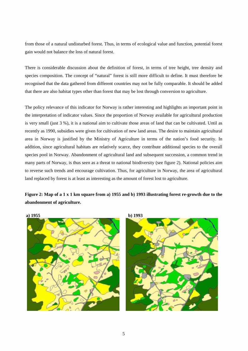
The policy relevance of this indicator for Norway is rather interesting and highlights an important point in

the interpretation of indicator values. Since the proportion of Norway available for agricultural production

is very small (just 3 %), it is a national aim to cultivate those areas of land that can be cultivated. Until as

recently as 1990, subsidies were given for cultivation of new land areas. The desire to maintain agricultural

area in Norway is justified by the Ministry of Agriculture in terms of the nation’s food security. In

addition, since agricultural habitats are relatively scarce, they contribute additional species to the overall

species pool in Norway. Abandonment of agricultural land and subsequent succession, a common trend in

many parts of Norway, is thus seen as a threat to national biodiversity (see figure 2). National policies aim

to reverse such trends and encourage cultivation. Thus, for agriculture in Norway, the area of agricultural

land replaced by forest is at least as interesting as the amount of forest lost to agriculture.

Figure 2: Map of a 1 x 1 km square from a) 1955 and b) 1993 illustrating forest re-growth due to the

abandonment of agriculture.

a) 1955 b) 1993

6

In countries with a greater proportion of agricultural land and small area of forest, say for example

Denmark with its 65 % agricultural land, the loss of forest areas to agriculture would be considered a

negative trend and the reversion of agricultural land to natural forest would be considered positive for

biological diversity. How will the reporting of indicators take into account the different goals suitable for

the different OECD member countries? (see below).

The habitat matrix indicator is an interesting attempt to link biological diversity with land types. To

calculate this indicator, the degree of dependence of many different species on different agricultural land

types must be identified, allowing assessment of which species are most likely to benefit from, or be

adversely affected by, observed changes in land cover. The indicator can be calculated based on the

collation and ordering of existing data on species biology and ecology, avoiding the need for detailed

species monitoring data that currently do not exist for many OECD countries, including Norway.

Calculation of the habitat matrix is seen as a very useful exercise to undertake. It will make explicit the

habitat value of different agricultural habitats in the various OECD countries and will highlight areas of

inadequate knowledge. However, there are many problems associated with this indicator, as reported in

chapter 6 of the OECD publication “Environmental indicators for agriculture: methods and results”. Not

least, the indicator will only be as good as the land cover/land use data used for its calculation. It is the

combination of land cover and land management practices that determine habitat quality and thus value to

biological diversity. If information on land cover/land use is too coarse, the indicator will be of little value.

For example, it would be insufficient to define the habitat suitability of “pasture” without recognising the

importance of grazing intensity, fertiliser application etc. Once the most important agricultural habitat

types have been identified, it would be more straightforward to simply monitor the area of these habitat

types. The theoretical link to potential species lists and habitat use units adds little extra meaning, and may

in some respects be misleading, by implying a level of species monitoring where in practice there may be

none. (In this respect the Natural Capital Index proposed by the Netherlands is better, being based on

actual species data).

In trying to add ecological meaning to measurements of the area of different land types, farming system

has been suggested as a very coarse-scale indicator of habitat quality. There are, however, also limitations

to the degree to which farming system can reflect quality. For the first, even though one farming system

may generally be more species-rich than another, the complement of species (i.e. which species are

present) will be different in the different systems such that interpreting whether changes are for the better

7

or worse may be difficult. Similarly, whilst organic agriculture has a set of clearly defined standards to

follow and checks to ensure that these are upheld, other farming systems may vary immensely with regard

to management and hence their quality as habitat. In addition, natural environmental conditions will lead to

different levels of biodiversity even in areas having the same management. To assess quality, some field

monitoring at the species level is essential. Ideally this intensive monitoring should be done in close

connection with extensive monitoring so that estimates can be more easily made of the connection between

changes in land use and changes in quality.

FRAGMENTATION / HETEROGENEITY

One type of change that is not captured by any of the proposed indicators, is changes in the spatial

structure of agricultural habitats. Landscape ecological theory suggests that it is not only the amount and

quality of habitat that affects biological diversity but also the spatial arrangement of this habitat (Forman,

1995).

A simple way to monitor fragmentation of agricultural land, or fragmentation of natural areas by

agriculture, is to monitor the size of coherent units of agricultural land and natural areas within agricultural

land. Average size will provide an easily interpretable indicator that is applicable at a range of scales

(local, regional and national).

In Norway, for example, the average size of arable fields ranges from just over 2 ha in the most intensively

cultivated counties, to around 1 ha in counties that are more marginal for agriculture. These field sizes are,

of course, very small compared to those of many OECD countries. The indicator provides information

about the landscape structure associated with Norwegian agriculture that cannot be assessed simply from

data about the total area of agricultural land.

Generally, it is in those countries with large areas of highly intensive agro-ecosystems that the problem of

loss of biodiversity has been greatest and the issue of fragmentation of habitats has been most severe. In

such countries, it is the natural habitats which form islands amidst a sea of agricultural land. In Norway, it

is commonly the agricultural areas which are fragmented, forming patches in an expanse of forest.

In order to achieve long-term sustainability in agriculture, the aim should be to improve the entire

countryside not just to preserve isolated islands of habitat. Similarly, to preserve agro-ecosystems such as

species-rich hay meadows, cultivated patches of the landscape should not become too isolated from one

8

another. It is thus important in both cases that indicators should incorporate the entire landscape, not just

the most valued ecosystems.

One indicator for the entire agricultural landscape that is in use in Norway, is a simple indicator of

landscape heterogeneity (Fjellstad et al., 2001). The heterogeneity index (Hix) was designed to distinguish

between ‘large-scaled landscapes’ with few elements per unit area, and ‘small-scaled landscapes’ with

many elements per unit area. Hix can therefore be seen as a measure of grain-size (sensu Wiens, 1989).

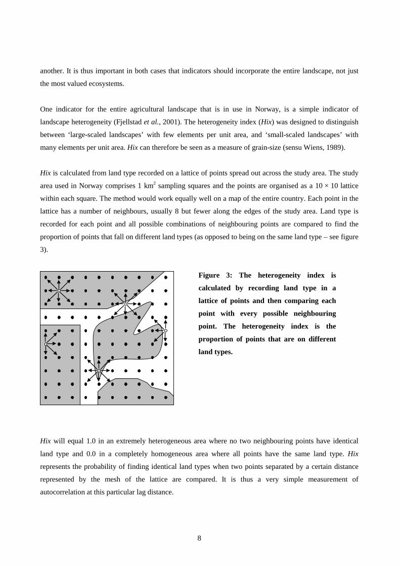
Hix is calculated from land type recorded on a lattice of points spread out across the study area. The study

area used in Norway comprises 1 km2 sampling squares and the points are organised as a 10 × 10 lattice

within each square. The method would work equally well on a map of the entire country. Each point in the

lattice has a number of neighbours, usually 8 but fewer along the edges of the study area. Land type is

recorded for each point and all possible combinations of neighbouring points are compared to find the

proportion of points that fall on different land types (as opposed to being on the same land type – see figure

3).

Figure 3: The heterogeneity index is

calculated by recording land type in a

lattice of points and then comparing each

point with every possible neighbouring

point. The heterogeneity index is the

proportion of points that are on different

land types.

Hix will equal 1.0 in an extremely heterogeneous area where no two neighbouring points have identical

land type and 0.0 in a completely homogeneous area where all points have the same land type. Hix

represents the probability of finding identical land types when two points separated by a certain distance

represented by the mesh of the lattice are compared. It is thus a very simple measurement of

autocorrelation at this particular lag distance.

9

Figure 4: Two example squares from the 3Q monitoring programme for agricultural landscapes,illustrating differences in

• land type diversity -Shannon’s diversity index: a) = 1.60 b) = 2.18• spatial structure -Heterogeneity index: a) = 0.23 b) = 0.77

a) b)

The heterogeneity index is clearly dependent on the spacing of the points used in its calculation. In

addition, the heterogeneity index, and indeed any index of spatial structure, will be highly dependent on the

mapping system used to generate index values, both in terms of the map legend (classification system) and

the mapping scale. Data will only be directly comparable (in time or in space) if the same methods are used

in calculating the index.

It should be emphasised that, whilst indicators of spatial structure provide objective descriptions of present

day agricultural landscapes and can describe changes in the spatial configuration of these landscapes over

time, more research is needed to enable interpretation of the indicators and it is stressed that great care

must be taken when trying to apply the figures for these indicators (e.g. heterogeneity and diversity). An

increase in the value of a given indicator of spatial structure may be a positive development in some areas,

but a negative development in other areas. Interpretation of changes will depend upon the history of the

landscape, present status and the “desired” landscape for the future.

For example, an increase in landscape heterogeneity in a coastal heath landscape may be considered a

negative change, as scrub and forest regenerate following cessation of grazing, and an ecosystem and

cultural heritage loses its specific character. On the other hand, an increase in heterogeneity of a large-

10

scale, intensively farmed arable area may represent the achievement of goals associated with

environmental enhancement, such as the establishment of grass banks to reduce erosion and increase the

occurrence of natural enemies of crop pests. In terms of biodiversity, a change in landscape heterogeneity

may be positive for some species and negative for other species within the same landscape.

Changes in heterogeneity and other structural indices should therefore be interpreted in a wider context and

to answer clearly defined questions. Use within a landscape typology may assist interpretation if clear

goals can be set for the direction and degree of change that is acceptable/desirable in an area. To some

extent, landscape heterogeneity and diversity, as objective descriptors, may also be useful in validating a

landscape typology, since these structural qualities are important components of landscape character.

However, care must be taken to standardise scale of measurement, since a landscape pattern will produce

very different heterogeneity or diversity values depending on the size of the sample units (i.e. dependent

upon whether the entire pattern is sampled or only a part of it).

As a general rule, the interpretation of landscape indices requires an understanding both of what the indices

describe and how this information relates to specific environmental targets. The indices cannot tell us how

best to manage the landscape, only how well we are achieving pre-defined targets.

DIFFERENT GOALS IN DIFFERENT LANDSCAPES

The indicators that have been proposed are relatively straightforward descriptions of aspects of the

agricultural landscape that are considered to be important for biological diversity. To date, however, there

has been little discussion of the fact that these indicators may have different significance in different

regions.

Take for example, the issue of loss of forest area to agriculture or re-growth of forest on agricultural land.

This particular issue of intensification versus extensification is a topic that has been raised frequently in

OECD discussions. The trends of change that are typical for these two opposing processes may easily mask

one another in national indicator estimates; a strong argument for a more regional presentation of indicator

values and targets.

To illustrate this point, the area of land under agriculture in Norway has declined by 8 % since 1939.

However, regional differences are great due to differences in natural conditions for farming. So for

example, the area of agriculture has increased by 2 % in an intensively cultivated municipality of South-

11

Eastern Norway (Rakkestad) but has declined by 36 % in a mountainous municipality (Hjartdal) with less

favourable topographic and climatic conditions.

Similarly, for some specific landscape types, an increase in biodiversity may reflect undesirable changes in

the landscape. When agricultural land is abandoned, for example, species diversity often increases in the

earlier stages of abandonment, but later declines. Certain habitat types, such as heath-land, are species

poor, yet contribute particular species to the national species pool that otherwise would not occur.

For indicators to be useful, they must be used at a resolution that enables observed changes in state to be

linked to driving forces and pressures. Whilst indicator calculation by regions may be undesirable for

international reporting at the level of the OECD, it may be worth considering a grouping of countries

according to broad similarities in landscape type and in environmental goals.

CONCLUSIONS

Although the proposed indicators have their limitations, they are measures that it is realistic to obtain for

the OECD countries. It must be accepted that there will be variations in definitions, and in the resolution at

which data are gathered. The most important point is to monitor and report relative changes over time

rather than actual numbers and amounts. Clearly it is easier for a country to project a positive image by

making a small change to a small total area, compared with the same change or greater on a larger total

area, and this should be recognised in reporting. It is also vital that the definitions used in data collection

are explicitly presented and that every attempt is made to point out where data are not comparable.

There have been many attempts to create international standards for mapping land cover, land use and

biotope cover, such as the Land Cover Classification System (di Gregorio and Hansen, 2000), CORINE

(http://reports.eea.eu.int/), EUNIS (http://mrw.wallonie.be/dgrne/sibw/EUNIS/home.html) etc. One reason

that these have not been universally accepted is that, in trying to be useable by all they may become less

suited for national use. Definitions, such as those for forest, are often relevant and appropriate for the areas

for which they were intended to be used and are useful for regional comparisons within a country. In

addition, once nationally useful data are being gathered, according to nationally appropriate methods, it

may seem unreasonable to use resources to gather the data again in a different way, simply to be able to

report internationally.

12

It therefore seems appropriate to accept some methodological differences between nations and to begin to

report indicators for wildlife habitats. The sooner this begins, the sooner we will have some indication of

the effects of agricultural activities on agricultural ecosystems.

REFERENCES

Anon. (1999). Identification des habitats agricoles semi-naturels et des habitats naturels non-exploites dans

l’ecosysteme agricole. OECD Expert meeting on biodiversity, wildlife habitats and landscape, 3rd

– 5th May 1999. Room document no. 9, Switzerland.

di Gregorio, A. and Hansen, L.J.M. (2000). Land Cover Classification System (LCCS): Classification

concepts and user manual. Rome: FAO. http://www.lccs-info.org/

Fjellstad, W.J. and Dramstad, W.E. (1999). “Patterns of change in two contrasting Norwegian agricultural

landscapes”. Landscape and Urban Planning 45: p. 177-191.

Fjellstad, W.J., Dramstad, W.E., Strand, G.-H. and Fry, G.L.A. (2001). “Heterogeneity as a measure of

spatial pattern for monitoring agricultural landscapes”. Norwegian Journal of Geography 55: 71-

76.

Forman, R.T.T. (1995). Land Mosaics: The ecology of landscapes and regions. Cambridge University

Press, Cambridge.

MacDonald, D., Crabtree, J.R., Wiesinger, G., Dax, T., Stamou, N., Fleury, P., Gutierrez Lazpita, J. and

Gibon, A. (2000). “Agricultural abandonment in mountain areas of Europe: Environmental

consequences and policy response”. Journal of Environmental Management 59: 47-69.

OECD. (2001) “Environmental indicators for agriculture – Volume 3: methods and results”. Paris: OECD

Publications.

White Paper No. 19. (1999). Om norsk landbruk og matproduksjon. Ministry of Agriculture, Oslo.

White Paper No. 1. (2001). Nasjonalbudsjettet. Ministry of Agriculture, Oslo.

Wiens, J.A. (1989). “Spatial scaling in ecology”. Functional Ecology 3, 385-398.