plotting openfoam residuals and forces in real...

~ 1 ~

Plotting OpenFoam residuals and forces in real time

Reference is made to an earlier paper titled Plotting OpenFoam forces and moments in real time. Readers

are encouraged to review that paper before studying this one. The earlier paper describes how

OpenFoam’s case directories work, how Python3 can be installed, how Python3 scripts work, and such

like, which I will not repeat below.

The earlier paper described a Python3 program named “fplot.py”, where “fplot” is an acronym for

“plotting forces”. If this program has been copied into the active OpenFoam case directory, it can be run

in real time, even while OpenFoam continues its calculations, to plot the history through the iterations of

a spatial component of a force or moment. Usage of fplot.py assumes that the “controlDict” for the case

contains a function instructing OpenFoam to write the forces and moments to a file at the end of every

iteration. When run, fplot.py examines the files (there can be more than one) which contain the force and

moment data, collates the information and plots the variable specified by the user.

fplot.py is limited to plotting forces and moments. It is also limited to plotting only one force or moment

component at a time. The program described in this paper removes both limitations. It can plot residuals

as well as forces and moments. In fact, it can plot any of the numerical data which OpenFoam generates,

including variables like time step continuities. I have used the name “plotAll.py” for the program

described in this paper, the name being short for “plot all OpenFoam data”. Like fplot.py, plotAll.py is a

Python3 program which is copied into the active OpenFoam case directory and run from a new terminal

window opened in the case directory.

Source of the data

plotAll.py gets its data from a file which holds a copy of the terminal screen output which OpenFoam

generates. When an OpenFoam solver like simpleFoam is executed, it writes continuous text to the

terminal screen. This text can be made available to other programs quite easily. Here, and elsewhere

below, I will assume that the usual prompt given for a new terminal window is “jim@jim:~$”. I will also

assume that the OpenFoam case directory has the name “Case_120kph_5m_Mesh#A”, which happens to

reside in a directory named “Drafting” on the desktop. After a new terminal window is opened, the

sequence of steps needed to change into the case directory and to run a simpleFoam application is the

following. (I have colored the Linux-generated text in blue and the user’s typing in black.)

jim@jim:~$ cd Desktop/Drafting/Case_120kph_5m_Mesh#A

jim@jim:~/Desktop/Drafting/Case_120kph_5m_Mesh#A$ simpleFoam | tee ofLog.txt

The command in the first line changes the directory to the case directory. The command in the second

line begins the execution of simpleFoam. The vertical slash and following “tee” begin the execution of a

program which works like a T-joint in plumbing – it sends the text it receives to two destinations, the

terminal screen, as usual, but also to the file whose name is given. In the example shown, an exact copy

of the text which appears on the terminal screen will be sent to the text file named “ofLog.txt”. ofLog.txt

will be created in the case directory where it will appear as a sister file to plotAll.py.

The syntax given above is appropriate when the simulation commences at time step 0. If the case has run

before, but was terminated and is now being re-started, the appropriate syntax would be this:

jim@jim:~/Desktop/Drafting/Case_120kph_5m_Mesh#A$ simpleFoam | tee –a ofLog.txt

The “a” option tells the tee program that the text soon to be coming should be appended to file ofLog.txt

which already exists.

~ 2 ~

Time = 74

smoothSolver: Solving for Ux, Initial residual = 0.001088847, Final residual = 8.176141e-05, No Iterations 6

smoothSolver: Solving for Uy, Initial residual = 0.003432152, Final residual = 0.0002506418, No Iterations 6

smoothSolver: Solving for Uz, Initial residual = 0.004479452, Final residual = 0.0003201872, No Iterations 6

GAMG: Solving for p, Initial residual = 0.02337899, Final residual = 0.0008043688, No Iterations 2



GAMG: Solving for p, Initial residual = 0.001157861, Final residual = 8.520689e-05, No Iterations 1

GAMG: Solving for p, Initial residual = 0.0002718626, Final residual = 2.288669e-05, No Iterations 2

time step continuity errors : sum local = 1.079882e-05, global = 3.552218e-08, cumulative = 0.002264786

smoothSolver: Solving for epsilon, Initial residual = 0.0006579817, Final residual = 5.450659e-05, No

Iterations 3

bounding epsilon, min: -0.007851726 max: 81067.49 average: 71.1994

smoothSolver: Solving for k, Initial residual = 0.001858562, Final residual = 0.000115734, No Iterations 4

ExecutionTime = 8545.98 s ClockTime = 9225 s

forces output:

forces(pressure, viscous)((825.5403 -580.248 -0.4527491) (16.02664 1.801927 -0.04621459))

moment(pressure, viscous)((3.037819 1.022001 -26224.27) (-0.0751561 1.973306 62.52686))

forces output:

forces(pressure, viscous)((6047.589 612.475 -65.64116) (85.81894 5.154761 0.2131515))

moment(pressure, viscous)((-94.3312 1608.879 7255.268) (0.3856533 0.2739873 -121.9552))

Format of the data

The user will have to change the code in plotAll.py so that it is consistent with the format of the output

which OpenFoam generates for his application. The format will vary from one application to another but,

often, one application will involve many cases all of which have the same format. The description I will

give below assumes that the output for each iteration has the following format.

This output was produced by simpleFoam using the k-ε turbulence model. The pressure was solved using

four non-orthogonal correctors. There happen to be two separate objects in the flow and the controlDict

contains two functions by which the forces and moments on the two objects are calculated separately.

When plotAll.py is run, it scans through ofLog.txt looking for the start of all time steps. plotAll.py looks

for the key phrase “Time = “. This key phrase has been highlighted in yellow in the text above. Once it

finds the start of a new iteration, plotAll.py begins to parse the following text, looking for other key

phrases the user has specified. These key phrases should uniquely identify the numeric fields in which

the user is interested. For example, the key phrase “Ux, Initial residual = “, which is also

highlighted in yellow in the text above, uniquely identifies the numeric field containing the initial residual

for the -component of the velocity.

If the next key phrase is “p, Initial residual = “, then plotAll.py will find the initial residual of the

first GAMC iteration of the pressure equation.

If the next key phrase is “global = “, then plotAll.py will find the global time step continuity error.

If the next key phrase is “forces(pressure, viscous) ((“, then plotAll.py will find the -component

of the pressure force acting on the first object.

If the next key phrase is “) (“, then plotAll.py will find the -component of the moment from the

pressure forces acting on the first object.

If the next key phrase is “ “ (a single blank), then plotAll.py will find the -component of the moment

from the pressure forces acting on the first object.

This is the single blank.

~ 3 ~

plotAll.py scans the text from beginning to end. The goal when choosing the key phrases is to specify

them so that plotAll.py is directed to the text which immediately precedes the numeric field which the

user may want plotted.

Notes:

1. plotAll.py does not scan the ofLog.txt file directly. When it starts running, plotAll.py copies

ofLog.txt into a temporary file named temp.txt. The copy operation is done quickly and avoids

the conflict which would arise if plotAll.py was parsing ofLog.txt at a time when tee wanted to

write the results from the next iteration into it.

2. Just because a numeric field has been identified by a key phrase does not mean that it has to be

plotted. However, the user should designate key phrases for any numeric fields which he may

want to plot.

3. So that it does not become confused by line feeds or carriage returns at the ends of lines,

plotAll.py combines the output text for each iteration into a single string, where the line-end

character(s) are replaced by single blank spaces.

Naming the numeric fields

The user will also need to specify a name for each numeric field of interest. This is the label which will

appear in the legend on the plot when this variable is plotted. The name should be descriptive and, to the

extent possible, short.

Variable names and key phrases used in the sample plots below

The variable names and key phrases are stored in two lists near the beginning of plotAll.py’s code. The

following extract from the code shows the 12 key phrases and variable names which were defined for the

sample plots which are shown below. They are based on the output text format shown above. They

select the six residuals and the pressure forces (only) acting on the two objects.

# Key phrases;

NumFields = 12

FieldNames = []

FieldNames.append("Ux, Initial residual = ")

FieldNames.append("Uy, Initial residual = ")

FieldNames.append("Uz, Initial residual = ")

FieldNames.append("p, Initial residual = ")

FieldNames.append("epsilon, Initial residual = ")

FieldNames.append("k, Initial residual = ")

FieldNames.append("forces(pressure, viscous)((")

FieldNames.append(" ")





# Variable names:

VariableNames = []

VariableNames.append("UxRes")

VariableNames.append("UyRes")

VariableNames.append("UzRes")

VariableNames.append("pRes")

VariableNames.append("epsRes")

VariableNames.append("kRes")

VariableNames.append("FxVan")

VariableNames.append("FyVan")

VariableNames.append("FzVan")

VariableNames.append("FxTT")

VariableNames.append("FyTT")

VariableNames.append("FzTT")

~ 4 ~

The user will need to amend these two lists for his application so that they identify the numeric fields

which he intends to plot.

A sample plot or two

Let me leap ahead and give a sample plot. The following plot shows the base-10 logarithms of the six

residuals for iterations #100 through #750 of a simpleFoam case which did not converge.

By default, plotAll.py uses the name of the case directory as the title, puts the legend in the lower-left

corner and uses the time step or iteration number for the horizontal axis. An “(R)” after a variable’s name

in the legend indicates that it is plotted with respect to the right-side vertical axis. In this plot, the base-10

logarithms of all six variables are plotted with respect to the right-side vertical axis. Contrast that with

the following plot, in which only three of the residuals are plotted, but the physical variable FyVan (the -

direction pressure force on one of the objects) is also plotted.

In the following plot, the base-10 logarithms of the three selected residuals are plotted with respect to the

right-axis, but FyVan is plotted with respect to the left-side vertical axis. By default, plotAll.py uses thick

lines to render the curves for variables plotted with respect to the right-side vertical axis and thin lines to

render variables plotted with respect to the left-side vertical axis.

Placing the legend in the lower-left corner can be provoking at times. The user can specify that the

legend be placed in one of the other three corners, but cannot put the legend in a white box on top. Like

~ 5 ~

Python3, gnuplot is an interpreter, which executes its code line-by-line from beginning to end. The

legend is rendered at the same time as the curves are drawn, so the curves and legend are rendered in the

same front-to-back order as the code generated them. gnuplot cannot retrace its steps.

plotAll.py displays a command menu on the terminal screen.

When plotAll.py was executed for the case

plotted above, the initial menu looked like

this.

By default, plotAll.py will plot the last 100

iterations or, if there are less than 100

iterations, that lesser number of iterations.

The menu lists all of the defined variable

names and a note about what it intends to

do with them. Each defined variable name

has a cardinal number, starting from 0, by

which the user will identify it.

~ 6 ~

There are seven menu choices. Those with a “#” require that the user enter a whole number (0, 1, 2 …) as

part of his entry.

To plot UxRes, for example, the user would type “tp 0” in response to the “Enter selection: “

prompt, which will have the following result.

The command “tp 0” toggled the plot flag

for this variable. It will now be plotted.

By default, it will be plotted with respect to

the left-side axis. And, by default, it will

be plotted using the original numeric

values, as opposed to base-10 logarithms.

The “tp 0” is a toggle. Typing it in again

in response to the “Enter selection: “

prompt will cause plotAll.py not to plot it.

The “ta” command is also a toggle. It toggles between the left-side axis and the right-side axis. Since

variable 0 (UxRes) is currently set to be plotted with respect to the left-side axis, entering “ta 0” in

response to the “Enter selection: “ prompt will cause it to be plotted with respect to the right-side

axis. The following screenshot shows this.

To toggle UxRes into base-10 logarithm

mode, the user would type “tl 0” in

response to the “Enter selection: “

prompt.

This is a clumsy form of GUI in that the

whole menu is re-written on the screen

every time the user enters a command.

But, it is hard to do much more than this

using Python3.

The “num” command is not a toggle. It is used to change the number of iterations which are plotted. As I

described above, the default number of iterations which plotAll.py will plot is 100. To plot from iteration

#100 to iteration #750, for example, the user would type “num 650” in response to the “Enter

selection: “ prompt. This will case plotAll.py to plot the last 650 iterations, in other words, from #100

to #750.

~ 7 ~

Before describing the remaining commands, note the following screenshot. It shows the selections I

made to produce the second plot set out above, of three residuals and FyVan.

The “go” command is the command which causes plotAll.py to proceed with the plotting. Like the earlier

program fplot.py, plotAll.py generates a data file containing the columns of data which the user has

selected. This data file is a temporary file, and is saved with the name “plotfile.dat”. plotAll.py also

generates a gnuplot script file with the name “gnuscript.txt”. It, too, is a temporary file. If at any time,

the user spots files with the names “temp.txt”, “plotfile.dat” or “gnuscript.txt” somewhere in the case

directory, they can be deleted without concern. They are all temporary files.

The “ex” command ends plotAll.py and closes its terminal window.

The “re” command deserves special mention. I described above how plotAll.py does not read and parse

the ofLog.txt file directly, but creates a copy called “temp.txt” first. plotAll.py will use data from the

temp.txt file until it is told to refresh the data, which it will do by making a new copy of the current

ofLog.txt file. I often use the following procedure. Early in the course of an OpenFoam run, I invoke

plotAll.py and set up a template for a plot, with the residuals and forces I expect will bear watching.

From time-to-time during the run, it is an easy matter to come back to the computer, refresh the data using

“re” and then plot the data using “go”.

One last word: color. By default, gnuplot assigns different colors to each variable on a plot. The colors it

chooses do not always show up as well as one might like. Furthermore, when a plot uses both vertical

axes, it is possible and sometimes better to re-use certain colors. plotAll.py handles this matter as

follows. The code defines two lists of colors, one for the left-side vertical axis and one for the right-side

vertical axis. The user can specify the colors and their order. As it plots the variables, plotAll.py runs

down these two lists and instructs gnuplot which ones to use.

Appendix “A” is a listing of the program plotAll.py.

March 2013

Jim Hawley

An e-mail setting out errors and omissions would be appreciated.

~ 8 ~

Appendix “A”

Listing of plotAll.py

# This is a Python program designed to plot selected numbers from a text file

# which is a verbatim log of the output on the terminal screen from running an

# OpenFoam program. Any quantity which is sent to the terminal screen, and so

# copied into the text file, is available for plotting. The horizontal axis

# will always be the time step number; both vertical axes can be used to plot

# any numerical fields which appear in the log file.

# Assumptions:

# 1. That this file is named "plotAll.py";

# 2. That this file is located in the case directory;

# 3. That an OpenFoam job is running in a terminal window; and

# 4. That the OpenFoam job was initiated using "*Foam | tee ofLog.txt",

# with the appropriate * substitution for simpleFoam, picoFoam, icoFoam, etc.

# Invocation:

# 1. Open a second terminal window;

# 2. Change directory to the case directory;

# 3. Type the command "python3 plotAll.py".

# File names:

InputFileName = "ofLog.txt" # File containing a copy of the screen output

TempFileName = "temp.txt" # A temporary file

PlotFileName = "plotfile.dat" # File with data selected for plotting

GnuFileName = "gnuscript.txt" # File with gnuplot script

# List of colors for variables plotted w.r.t. the left axis

ColorNamesL= []

ColorNamesL.append(" lc rgb 'black' ")

ColorNamesL.append(" lc rgb 'red' ")

ColorNamesL.append(" lc rgb 'green' ")

ColorNamesL.append(" lc rgb 'blue' ")

ColorNamesL.append(" lc rgb 'magenta' ")

ColorNamesL.append(" lc rgb 'pink' ")

ColorNamesL.append(" lc rgb 'grey' ")

ColorNamesL.append(" lc rgb 'aquamarine' ")

ColorNamesL.append(" lc rgb 'lightgreen' ")

ColorNamesL.append(" lc rgb 'cyan' ")

# List of colors for variables plotted w.r.t. the right axis

ColorNamesR= []

ColorNamesR.append(" lc rgb 'black' ")

ColorNamesR.append(" lc rgb 'red' ")

ColorNamesR.append(" lc rgb 'green' ")

ColorNamesR.append(" lc rgb 'blue' ")

ColorNamesR.append(" lc rgb 'magenta' ")

ColorNamesR.append(" lc rgb 'pink' ")

ColorNamesR.append(" lc rgb 'grey' ")

ColorNamesR.append(" lc rgb 'aquamarine' ")

ColorNamesR.append(" lc rgb 'lightgreen' ")

ColorNamesR.append(" lc rgb 'cyan' ")

# Key phrases:

# The following strings are the identifying phrases this program should search for as

# it parses each time step in the screen output. The phrases must be unique. They must

# also be sufficiently complete to enable the program to identify the selected field as

# it parses the time step sequentially from beginning to end. There must be one field

# name for each set of figures which may be plotted. The search phrase for the time

# step will always be "Time = ".

NumFields = 12

FieldNames = []

FieldNames.append("Ux, Initial residual = ")

FieldNames.append("Uy, Initial residual = ")

~ 9 ~

FieldNames.append("Uz, Initial residual = ")

FieldNames.append("p, Initial residual = ")

FieldNames.append("epsilon, Initial residual = ")

FieldNames.append("k, Initial residual = ")







# Variable names:

# The following short strings are the names by which the fields will be referred in the

# plot. There must be one variable name for each set of figures which may be plotted.

# The time step will always have the name "Time".

VariableNames = []

VariableNames.append("UxRes")

VariableNames.append("UyRes")

VariableNames.append("UzRes")

VariableNames.append("pRes")

VariableNames.append("epsRes")

VariableNames.append("kRes")

VariableNames.append("FxVan")

VariableNames.append("FyVan")

VariableNames.append("FzVan")

VariableNames.append("FxTT")

VariableNames.append("FyTT")

VariableNames.append("FzTT")

# TimeStep vector and Value vector:

# The following vectors holds all of the values in a log file which could be plotted.

# Each time step in the log file will generate one entry in the TimeStep vector and

# NumFields entries in the Value vector. The entries for each time step in the Value

# vector will be in the same order as the search phrases defined in FieldNames[]. The

# total number of entries in ValueVector will be the number of complete time steps

# multiplied by NumFields.

TimeStepVector = []

ValueVector = []

# NumValuesToPlot specifies the length of the horizontal axis. NumValuesToPlot is the

# number of time steps which should be plotted. The procedure will plot the most recent

# NumValuesToPlot time steps or, if there are fewer time steps available, just those

# time steps which exist. The default is 100.

NumValuesToPlot = 100

# InstructionVector** specify the variables to plot and how to plot them. There are

# three InstructionVectors. Each is a list containing one position for each of the

# NumFields field names.

# InstructionVectorYN[] is "Y" or "N" depending on whether the corresponding

# field name should be plotted.

# InstructionVectorLR[] is "L" or "R" depending on whether the corresponding field

# name should be plotted on the left or the right axis.

# InstructionVectorOL[] is "O" or "L" depending on whether the corresponding field

# name should be plotted as original or logarithmic values.

InstructionVectorYN = []

InstructionVectorLR = []

InstructionVectorOL = []

for I in range(NumFields):

InstructionVectorYN.append("N")

InstructionVectorLR.append("L")

InstructionVectorOL.append("O")

~ 10 ~

#//////////////////////////////////////

#///// Function InitializeVectors /////

#//////////////////////////////////////

# This functions empties the lists TimeStepVector and ValueVector. This function is

# needed because the same variables are used every time a new plot is generated.

def InitializeVectors():

TimeStepVector[:] = []

ValueVector[:] = []

#/////////////////////////////////////////////

#///// Function SetToFirstTimeStep(fnum) /////

#/////////////////////////////////////////////

# This function reads file fnum up to the first line which begins with "Time = ".

# It stores the number following this phrase as the first entry in TimeStepVector[],

# that is, as TimeStepVector[0]. If no occurrence is found, the function terminates

# the application with an error message.

def SetToFirstTimeStep(fnum):

while True:

NextLine = fnum.readline()

if (NextLine == ""):

print("Error: End-of-file encountered.")

sys.exit()

else:

if (NextLine[0:7] == "Time = "):

# Isolate the number of the first time step.

NumberString = ""

for i in range(7, 1000):

if ( (NextLine[i:i+1] >= "0") and (NextLine[i:i+1] <= "9") ):

NumberString = NumberString + NextLine[i:i+1]

# Store NumberString as TimeStepVector[0].

TimeStepVector.append(int(NumberString))

break

#//////////////////////////////////////////

#///// Function GetNextTimeStep(fnum) /////

#//////////////////////////////////////////

# This function returns, as a string, the entire contents of the next time step in the

# file fnum. When called, the function begins to search from the current position in

# file fnum. The current position will be the start of a line where the previous line

# began with the phrase "Time = ". The number of the time step will already have been

# appended to TimeStepVector. From the current position onwards, this function builds

# the return string by adding each successive line, separated by a blank space from the

# previous contents. The building process ends when another line beginning with the

# phrase "Time = " is found, since this defines the start of the following time step.

# The number of the time step of the following time step is appended to TimeStepVector,

# leaving the file positioned for the next call to this function. Note that this

# function returns a null string if the end-of-file is reached before a complete time

# step string is built. Note also that the carriage return / line feed character at the

# end of each line in the text file is excluded when the line is added to the return

# string.

def GetNextTimeStep(fnum):

RetString = ""

# Search for the next line beginning with "Time = ".

while True:

NextLine = fnum.readline()

if (NextLine == ""):

return ""

else:

if (NextLine[0:7] == "Time = "):

# Isolate the number of the following time step.

NumberString = ""

for i in range(7, 1000):

if ( (NextLine[i:i+1] >= "0") and (NextLine[i:i+1] <= "9") ):

NumberString = NumberString + NextLine[i:i+1]

# Store NumberString as the next entry in TimeStepVector.

TimeStepVector.append(int(NumberString))

return RetString

~ 11 ~

else:

RetString = RetString + NextLine[0:len(NextLine)-1] + " "

#//////////////////////////////////////////////////

#///// Function ParseTimeStepString(tsstring) /////

#//////////////////////////////////////////////////

# This function parses a complete time step string, looking for the search phrases

# defined above as FieldNames[]. The search is linear, from the beginning to the

# end of the time step string. As each search phrase is found, the numerical value

# immediately following the search phrase is parsed out and appended to ValueVector[].

# If an error is encountered, the function terminates the application with an error

# message.

def ParseTimeStepString(tsstring):

# Replace all white spaces in the time step string with single blank spaces.

re.sub("\s\s+" , " ", tsstring)

# Search for the vertical axis search phases one-by-one.

for i in range(NumFields):

Location = tsstring.find(FieldNames[i])

if (Location < 0):

print("Error: The phrase " + FieldNames[i] + " was not found.")

sys.exit()

else:

tsstring = tsstring[Location + len(FieldNames[i]): len(tsstring)]

tstsring = tsstring.lstrip()

# Isolate the number at the start of tsstring.

NumberString = ""

for j in range(1000):

if ((tsstring[j:j+1] == "+") or

(tsstring[j:j+1] == "-") or

(tsstring[j:j+1] == ".") or

( (tsstring[j:j+1] >= "0") and (tsstring[j:j+1] <= "9") ) or

(tsstring[j:j+1] == "e")):

NumberString = NumberString + tsstring[j:j+1]

else:

tsstring = tsstring[j:len(tsstring)]

break

# Append the number to ValueVector[].

if (len(NumberString) <= 0):

print("Error: Field value is the null string")

sys.exit()

else:

ValueVector.append(float(NumberString))

return

# Imports

import math

import os

import re

import shutil

import subprocess

import sys

# Store the name of the case directory in variable CaseDir.

CaseDir = os.getcwd()

#//////////////////////////////

#///// Start of main loop /////

#//////////////////////////////

while True:

# Step #1: Ensure that the file "ofLog.txt" exists.

LogFileExists = False

fnames = os.listdir(CaseDir)

for fname in fnames:

if (os.path.isfile(fname)):

if (fname == InputFileName):

LogFileExists = True

~ 12 ~

if (LogFileExists == False):

print("Error: The log file " + InputFileName + " was not found.")

sys.exit()

# Step #2: Copy the log file into a temporary file.

try:

shutil.copyfile(InputFileName, TempFileName)

except:

print("Error: The log file could not be copied into a temporary file.")

sys.exit()

# Step #3: Open the temporary file containing the copy of the log file.

try:

FileNumber = open(TempFileName, "r")

except:

print("Error: Could not open the temporary file.")

sys.exit()

# Step #4: Position the temporary file to the start of the first time step.

InitializeVectors()

SetToFirstTimeStep(FileNumber)

# Step #5: Process the temporary file time step-by-time step, then close it.

while True:

TimeStepString = GetNextTimeStep(FileNumber)

if (TimeStepString == ""):

FileNumber.close()

break

else:

ParseTimeStepString(TimeStepString)

# Step #6: Display the number of time steps.

NumAvailableValues = int( len(ValueVector) / NumFields )

print(" ")

print("There are " + str(NumAvailableValues) + " time steps in the log.")

if (NumValuesToPlot > NumAvailableValues):

NumValuesToPlot = NumAvailableValues

print(" Will plot " + str(NumValuesToPlot) + " time steps.")

#/////////////////////////

#///// Start of menu /////

#/////////////////////////

while True:

# Step #7: Display the current plotting instructions.

print(" ")

DisplayString = ""

for I in range(NumFields):

DisplayString = " " + str(I) + ". " + VariableNames[I]

if (InstructionVectorYN[I] == "Y"):

DisplayString = DisplayString + " - to be plotted"

if (InstructionVectorLR[I] == "L"):

DisplayString = DisplayString + " on the left axis"

else:

DisplayString = DisplayString + " on the right axis"

if (InstructionVectorOL[I] == "O"):

DisplayString = DisplayString + ", original values"

else:

DisplayString = DisplayString + ", logarithmic values"

else:

DisplayString = DisplayString + " - do not plot"

print(DisplayString)

~ 13 ~

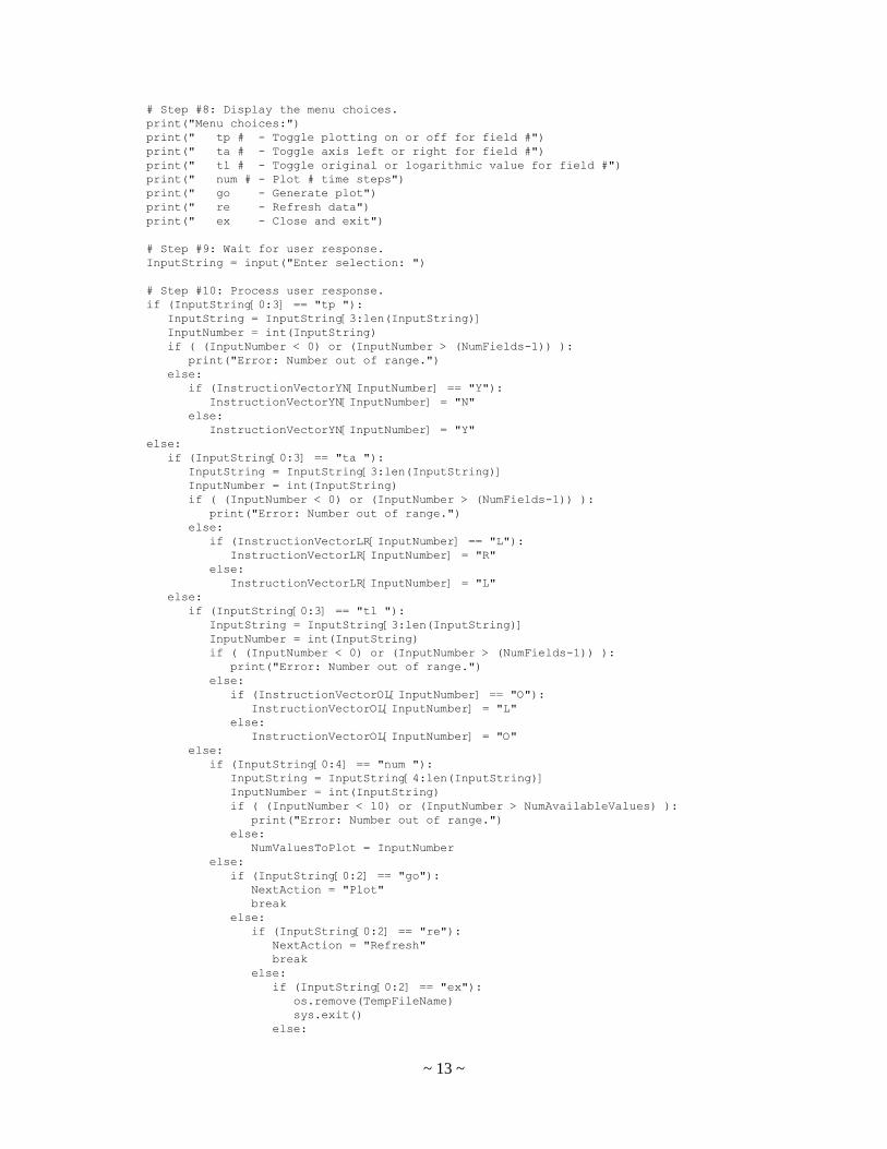
# Step #8: Display the menu choices.

print("Menu choices:")

print(" tp # - Toggle plotting on or off for field #")

print(" ta # - Toggle axis left or right for field #")

print(" tl # - Toggle original or logarithmic value for field #")

print(" num # - Plot # time steps")

print(" go - Generate plot")

print(" re - Refresh data")

print(" ex - Close and exit")

# Step #9: Wait for user response.

InputString = input("Enter selection: ")

# Step #10: Process user response.

if (InputString[0:3] == "tp "):

InputString = InputString[3:len(InputString)]

InputNumber = int(InputString)

if ( (InputNumber < 0) or (InputNumber > (NumFields-1)) ):

print("Error: Number out of range.")

else:

if (InstructionVectorYN[InputNumber] == "Y"):

InstructionVectorYN[InputNumber] = "N"

else:

InstructionVectorYN[InputNumber] = "Y"

else:

if (InputString[0:3] == "ta "):





else:

if (InstructionVectorLR[InputNumber] == "L"):

InstructionVectorLR[InputNumber] = "R"

else:

InstructionVectorLR[InputNumber] = "L"

else:

if (InputString[0:3] == "tl "):





else:

if (InstructionVectorOL[InputNumber] == "O"):

InstructionVectorOL[InputNumber] = "L"

else:

InstructionVectorOL[InputNumber] = "O"

else:

if (InputString[0:4] == "num "):



if ( (InputNumber < 10) or (InputNumber > NumAvailableValues) ):


else:

NumValuesToPlot = InputNumber

else:

if (InputString[0:2] == "go"):

NextAction = "Plot"

break

else:

if (InputString[0:2] == "re"):

NextAction = "Refresh"

break

else:

if (InputString[0:2] == "ex"):

os.remove(TempFileName)

sys.exit()

else:

~ 14 ~

print("Error: Unrecognizable response.")

if (NextAction == "Plot"):

#////////////////////////////////////////////////////

#///// Write data to be plotted to PlotFileName /////

#////////////////////////////////////////////////////

# Step #11: Open the plot data file.

try:

FileNumber = open(PlotFileName, "w")

except:

print("Error: Could not open the plot data file.")

sys.exit()

# Step #12: Write the selected fields for the selected time steps.

FirstValueToPlot = NumAvailableValues - NumValuesToPlot

for i in range(FirstValueToPlot, NumAvailableValues):

LineInPlotFile = str(TimeStepVector[i]) + " "

for j in range(NumFields):

if (InstructionVectorYN[j] == "Y"):

IndexInValueVector = (i * NumFields) + j

if (InstructionVectorOL[j] == "O"):

LineInPlotFile = LineInPlotFile + str(ValueVector[IndexInValueVector]) + " "

else:

if (ValueVector[IndexInValueVector] > 0):

LogValue = math.log10(ValueVector[IndexInValueVector])

else:

LogValue = -math.log10(-ValueVector[IndexInValueVector])

LineInPlotFile = LineInPlotFile + str(LogValue) + " "

FileNumber.write(LineInPlotFile + "\n")

# Step #13: Close the plot data file.

FileNumber.close()

#//////////////////////////////////

#///// Build the gnuplot file /////

#//////////////////////////////////

# Step #14: Open a file for the script to control gnuplot.

try:

FileNumber = open(GnuFileName, "w")

except:

print("Error: Could not open gnuplot script file.")

sys.exit()

# Step #15: Organize and write the gnuplot script.

FileNumber.write("# GnuPlot script file\n")

FileNumber.write("set autoscale # scale axes automatically\n")

FileNumber.write("unset log # remove any loraithmic scaling\n")

FileNumber.write("unset label # remove any previous labels\n")

FileNumber.write("unset mouse # do not display mouse co-ordinates\n")

FileNumber.write("set xtics auto # set xtics automatically\n")

FileNumber.write("set ytics auto # set ytics automatically\n")

FileNumber.write("set y2tics auto # set y2tics automatically\n")

FileNumber.write("set key bottom left\n")

FileNumber.write("set style data lines\n")

FileNumber.write("set grid\n")

TitleString = "Case directory is " + CaseDir

FileNumber.write("set title '" + TitleString + "'\n")

FileNumber.write("set xlabel 'Time or iteration'\n")

# Plot each selected field.

FileNumber.write("plot \\")

FileNumber.write("\n")

Column = 1

ColorL = -1 # Index for color of variables plotted w.r.t. the left axis

ColorR = -1 # Index for color of variables plotted w.r.t. the right axis

for i in range(NumFields):

~ 15 ~

if (InstructionVectorYN[i] == "Y"):

Column = Column + 1

if (Column != 2):

FileNumber.write(",\\")


if (InstructionVectorLR[i] == "L"):

ColorL = ColorL + 1

FileNumber.write(" '" + PlotFileName + "' using 1:" + str(Column) +

" axes x1y1 " + " linewidth 1 " + ColorNamesL[ColorL] +

" title '" + VariableNames[i] + " (L)'")

else:

ColorR = ColorR + 1

FileNumber.write(" '" + PlotFileName + "' using 1:" + str(Column) +

" axes x1y2" + " linewidth 3 " + ColorNamesR[ColorR] +

" title '" + VariableNames[i] + " (R)'")


# Step #16: Close the gnuplot script file.

FileNumber.close()

# Step #17 - Execute the gnuplot script.

GnuPlotProcess = subprocess.Popen("gnuplot -persist " + GnuFileName, shell = True)

os.waitpid(GnuPlotProcess.pid, 0)

# Step #18 - Delete the temporary files.

os.remove(PlotFileName)

os.remove(GnuFileName)

plotting openfoam residuals and forces in real...

Documents