PlSc 724 - FACTORIAL EXPERIMENTS

Factor - refers to a kind of treatment. Factors will be referred to with capital letters.

Level - refers to several treatments within any factor. Levels will be referred to with lower case letters. A combination of lower case letters and subscript numbers will be used to designate individual treatments (a0, a1, bo, b1, a0b0, a0b1, etc.) Experiments and examples discussed so far in this class have been one factor experiments. For one factor experiments, results obtained are applicable only to the particular level in which the other factor(s) was maintained. Example: Five seeding rates and one cultivar. A factorial is not a design but an arrangement. A factorial is a study with two or more factors in combination. Each level of a factor must appear in combination with all levels of the other factors. Factorial arrangements allow us to study the interaction between two or more factors. Interaction – 1) the failure for the response of treatments of a factor to be the same for each

level of another factor.

2) When the simple effects of a factor differ by more than can be attributed to chance, the differential response is called an interaction.

Examples of Interactions

0

1

2

3

4

5

a0 a1

Factor A

Dep

ende

nt v

aria

ble

b0

b1

0

1

2

3

4

5

a0 a1

Factor A

Dep

ende

nt v

aria

ble

b0

b1

No interaction (similar response) Interaction (diverging response)

1

0

1

2

3

4

5

a0 a1

Factor A

Dep

ende

nt v

aria

ble

b0

b1

01234567

a0 a1

Factor A

Dep

ende

nt v

aria

ble

b0b1

Interaction (crossover response) Interaction (converging response) Simple Effects, Main Effects, and Interactions Simple effects, main effects, and interactions will be explained using the following data set: Table 1. Effect of two N rates of fertilizer on grain yield (Mg/ha) of two barley cultivars.

Fertilizer Rate (B)

Cultivar (A) 0 kg N/ha (b0) 60 kg N/ha (b1)

Larker (a0) 1.0 (a0b0) 3.0 (a0b1)

Morex (a1) 2.0 (a1b0) 4.0 (a1b1) The simple effect of a factor is the difference between its two levels at a given level of the other factor. Simple effect of A at b0 = a1b0 - a0b0 = 2 - 1 = 1 Simple effect of A at b1 = a1b1 - a0b1 = 4 - 3 = 1 Simple effect of B at a0 = a0b1 - a0b0 = 3 - 1 = 2 Simple effect of B at a1 = a1b1 - a1b0 = 4 - 2 = 2

2

0

1

2

3

4

5

a0 a1

Factor A

Wei

ght

b0b1

0

1

2

3

4

5

b0 b1

Factor B

Wei

ght

a0a1

The main effect of a factor is the average of the simple effects of that factor over all levels of the other factor. Main effect of A = (simple effect of A at b0 + simple effect of A at b1) 2 = (1 + 1)/2 = 1 Main effect of B = (simple effect of B at a0 + simple effect of B at a1) 2 = (2 + 2)/2 = 2 The interaction is a function of the difference between the simple effects of A at the two levels of B divided by two, or vice-versa. (This works only for 2 x 2 factorials) A x B = 1/2(Simple effect of A at b1 - Simple effect of A at b0) = 1/2(1 - 1) = 0 or A x B = 1/2(Simple effect of B at a1 - Simple effect of B at a0) = 1/2(2 - 2) = 0

3

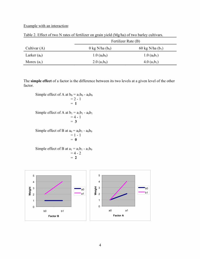
Example with an interaction: Table 2. Effect of two N rates of fertilizer on grain yield (Mg/ha) of two barley cultivars.

Fertilizer Rate (B)

Cultivar (A) 0 kg N/ha (b0) 60 kg N/ha (b1)

Larker (a0) 1.0 (a0b0) 1.0 (a0b1)

Morex (a1) 2.0 (a1b0) 4.0 (a1b1) The simple effect of a factor is the difference between its two levels at a given level of the other factor. Simple effect of A at b0 = a1b0 - a0b0 = 2 - 1 = 1 Simple effect of A at b1 = a1b1 - a0b1 = 4 - 1 = 3 Simple effect of B at a0 = a0b1 - a0b0 = 1 - 1 = 0 Simple effect of B at a1 = a1b1 - a1b0 = 4 - 2 = 2

0

1

2

3

4

5

b0 b1

Factor B

Wei

ght

a0a1

0

1

2

3

4

5

a0 a1

Factor A

Wei

ght

b0b1

4

The main effect of a factor is the average of the simple effects of that factor over all levels of the other factor. Main effect of A = (simple effect of A at b0 + simple effect of A at b1) 2 = (1 + 3)/2 = 2 Main effect of B = (simple effect of B at a0 + simple effect of B at a1) 2 = (0 + 2)/2 = 1 The interaction is a function of the difference between the simple effects of A at the two levels of B divided by two, or vice-versa. (This works only for 2 x 2 factorials) A x B = 1/2(Simple effect of A at b1 - Simple effect of A at b0) = 1/2(3 - 1) = 1 or A x B = 1/2(Simple effect of B at a1 - Simple effect of B at a0) = 1/2(2 - 0) = 1 Facts to Remember about Interactions

1. An interaction between two factors can be measured only if the two factors are tested together in the same experiment.

2. When an interaction is absent, the simple effect of a factor is the same for all levels of the

other factors and equals the main effect.

3. When interactions are present, the simple effect of a factor changes as the level of the other factor changes. Therefore, the main effect is different from the simple effects.

5

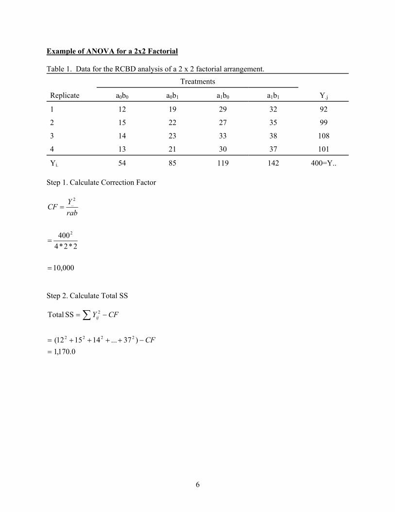
Example of ANOVA for a 2x2 Factorial Table 1. Data for the RCBD analysis of a 2 x 2 factorial arrangement. Treatments

Replicate a0b0 a0b1 a1b0 a1b1 Y.j

1 12 19 29 32 92

2 15 22 27 35 99

3 14 23 33 38 108

4 13 21 30 37 101

Yi. 54 85 119 142 400=Y.. Step 1. Calculate Correction Factor

000,10

2*2*44002

2..

=

=

=rabYCF

Step 2. Calculate Total SS

0.170,1)37...141512(

SS Total

2222

2

=−++++=

−= ∑

CF

CFYij

6

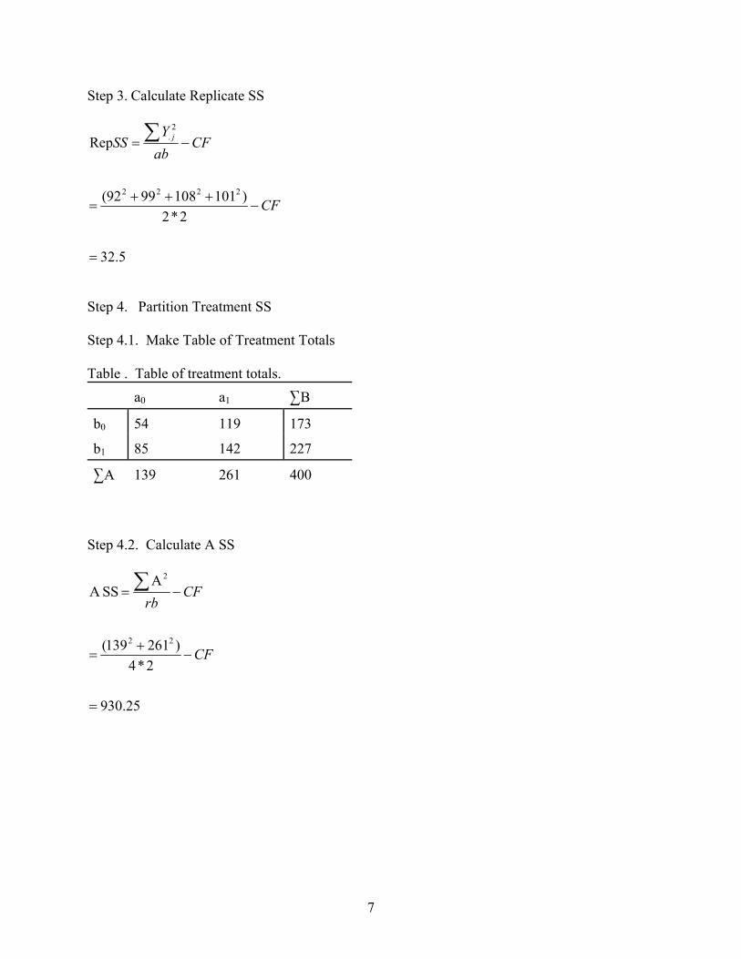
Step 3. Calculate Replicate SS

5.32

2*2)1011089992(

Rep

2222

2.

=

−+++

=

−= ∑

CF

CFabY

SS j

Step 4. Partition Treatment SS Step 4.1. Make Table of Treatment Totals Table . Table of treatment totals. a0 a1 3B

b0 54 119 173

b1 85 142 227

3A 139 261 400 Step 4.2. Calculate A SS

25.930

2*4)261139(

ASSA

22

2

=

−+

=

−= ∑

CF

CFrb

7

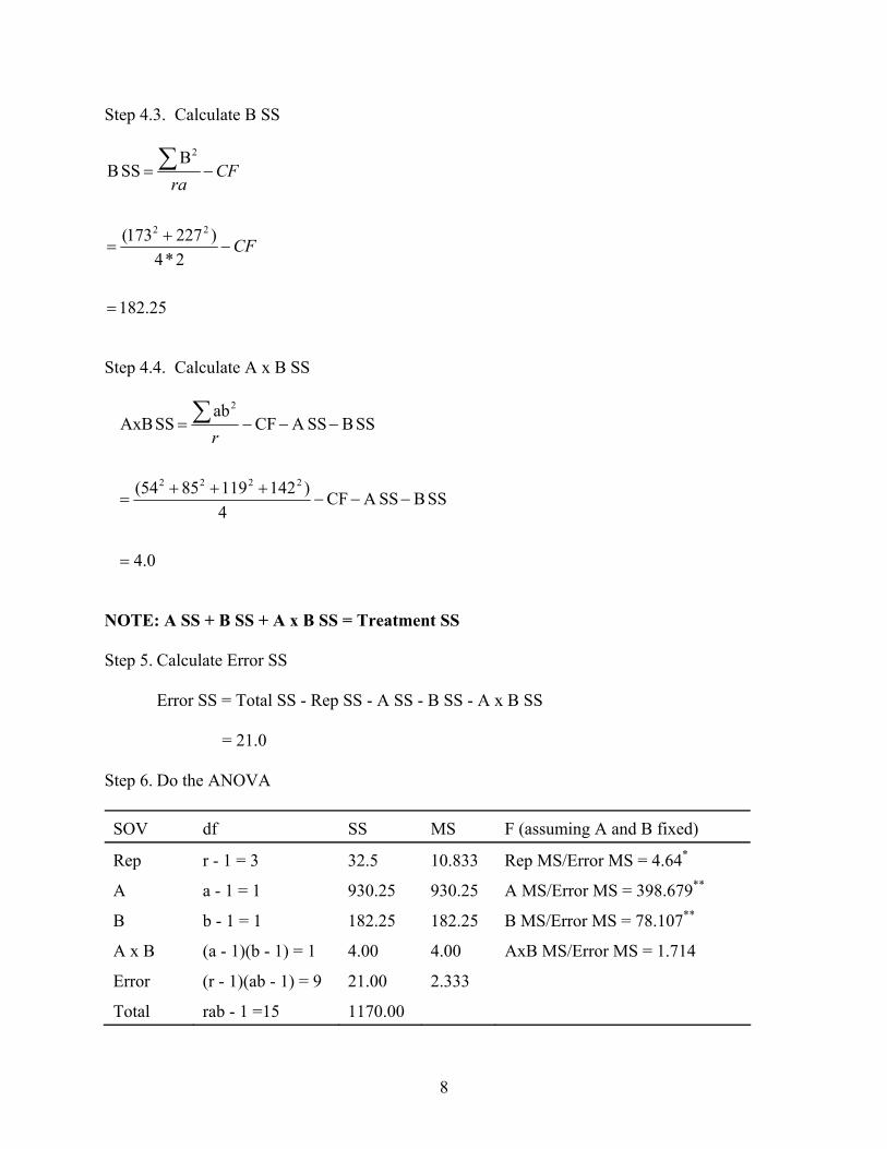
Step 4.3. Calculate B SS

25.182

2*4)227173(

BSS B

22

2

=

−+

=

−= ∑

CF

CFra

Step 4.4. Calculate A x B SS

4.0

SS BSSA CF4

)14211985(54

SS BSSA CFab

SS AxB

2222

2

=

−−−+++

=

−−−= ∑r

NOTE: A SS + B SS + A x B SS = Treatment SS Step 5. Calculate Error SS

Error SS = Total SS - Rep SS - A SS - B SS - A x B SS = 21.0 Step 6. Do the ANOVA SOV df SS MS F (assuming A and B fixed)

Rep r - 1 = 3 32.5 10.833 Rep MS/Error MS = 4.64*

A a - 1 = 1 930.25 930.25 A MS/Error MS = 398.679**

B b - 1 = 1 182.25 182.25 B MS/Error MS = 78.107**

A x B (a - 1)(b - 1) = 1 4.00 4.00 AxB MS/Error MS = 1.714

Error (r - 1)(ab - 1) = 9 21.00 2.333

Total rab - 1 =15 1170.00

8

Step 7. Calculate LDS’s (0.05) Step 7.1 Calculate LSDA

7.1

2*4)333.2(2262.2

rbMSError 2tA LSD .05/2;9df

=

=

=

Mean of treatment A averaged across all levels of B.

Treatment Mean a0 17.4 a a1 32.6 b

Step 7.2 Calculate LSDB

7.1

2*4)333.2(2262.2

raMSError 2tB LSD .05/2;9df

=

=

=

Mean of treatment B averaged across all levels of A.

Treatment Mean b0 21.6 a b1 28.4 b

9

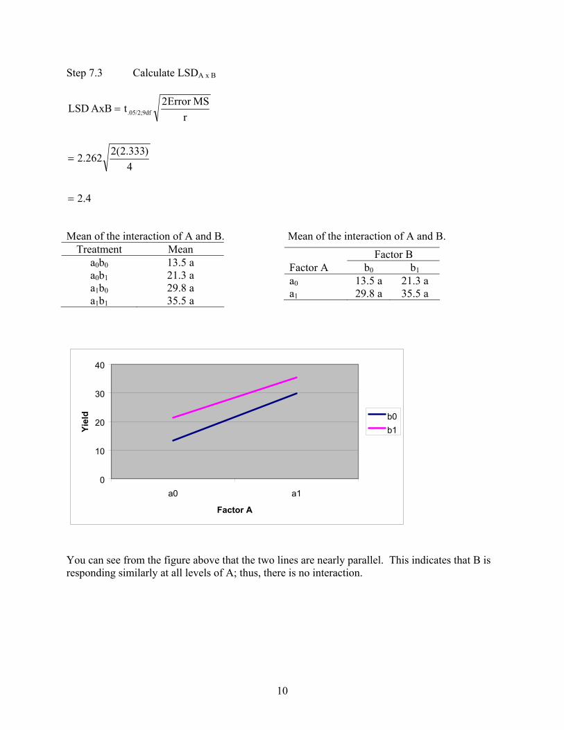
Step 7.3 Calculate LSDA x B

4.2

4)333.2(2262.2

rMSError 2tAxB LSD .05/2;9df

=

=

=

Mean of the interaction of A and B. Mean of the interaction of A and B.

Treatment Mean a0b0 13.5 a a0b1 21.3 a a1b0 29.8 a a1b1 35.5 a

Factor B Factor A b0 b1 a0 13.5 a 21.3 a a1 29.8 a 35.5 a

0

10

20

30

40

a0 a1

Factor A

Yiel

d b0b1

You can see from the figure above that the two lines are nearly parallel. This indicates that B is responding similarly at all levels of A; thus, there is no interaction.

10

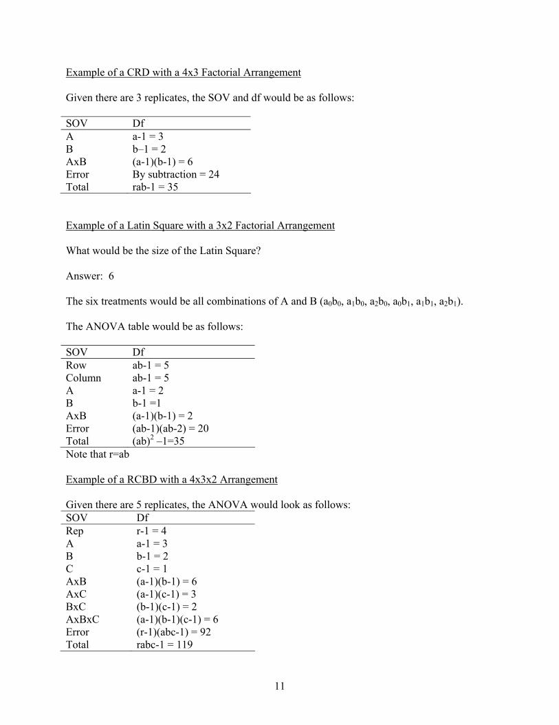
Example of a CRD with a 4x3 Factorial Arrangement Given there are 3 replicates, the SOV and df would be as follows: SOV Df A a-1 = 3 B b–1 = 2 AxB (a-1)(b-1) = 6 Error By subtraction = 24 Total rab-1 = 35 Example of a Latin Square with a 3x2 Factorial Arrangement What would be the size of the Latin Square? Answer: 6 The six treatments would be all combinations of A and B (a0b0, a1b0, a2b0, a0b1, a1b1, a2b1). The ANOVA table would be as follows: SOV Df Row ab-1 = 5 Column ab-1 = 5 A a-1 = 2 B b-1 =1 AxB (a-1)(b-1) = 2 Error (ab-1)(ab-2) = 20 Total (ab)2 –1=35 Note that r=ab Example of a RCBD with a 4x3x2 Arrangement Given there are 5 replicates, the ANOVA would look as follows: SOV Df Rep r-1 = 4 A a-1 = 3 B b-1 = 2 C c-1 = 1 AxB (a-1)(b-1) = 6 AxC (a-1)(c-1) = 3 BxC (b-1)(c-1) = 2 AxBxC (a-1)(b-1)(c-1) = 6 Error (r-1)(abc-1) = 92 Total rabc-1 = 119

11

In order to calculate the Sums of Squares for A, B, C, AxB, Ax C, BxC, and AxBxC, you will need to make several tables of treatment totals. The general outline of these tables is as follows: Table 1. Totals used to calculate A SS, B SS, and AxB SS. a0 a1 a2 a3 ∑B b0 a0b0 a1b0 b1 b2 ∑ A

Remember AxB SS = ( )rcab∑ 2

- CF – A SS – B SS

Table 2. Totals used to calculate A SS, C SS, and AxC SS. a0 a1 a2 a3 ∑C c0 a0c0 a1c0 c1 ∑ A

Remember AxC SS = ( )rbac∑ 2

- CF – A SS – C SS

Table 3. Totals used to calculate B SS, C SS, and BxC SS. b0 b1 b2 ∑C c0 b0c0 b1c0 c1 ∑B

Remember BxC SS = ( )rabc 2∑ - CF – B SS – C SS

Table 4. Values used to calculate Total SS, Rep SS, and AxBxC SS. Rep 1 Rep 2 Rep 3 ∑ ABC a0b0c0 a0b0c1

a0b1c0 … a3b1c1 ∑Rep

Remember AxBxC SS = ( )rabc∑ 2

- CF – A SS - B SS – C SS – AxB SS – AxC SS – BxC SS

12

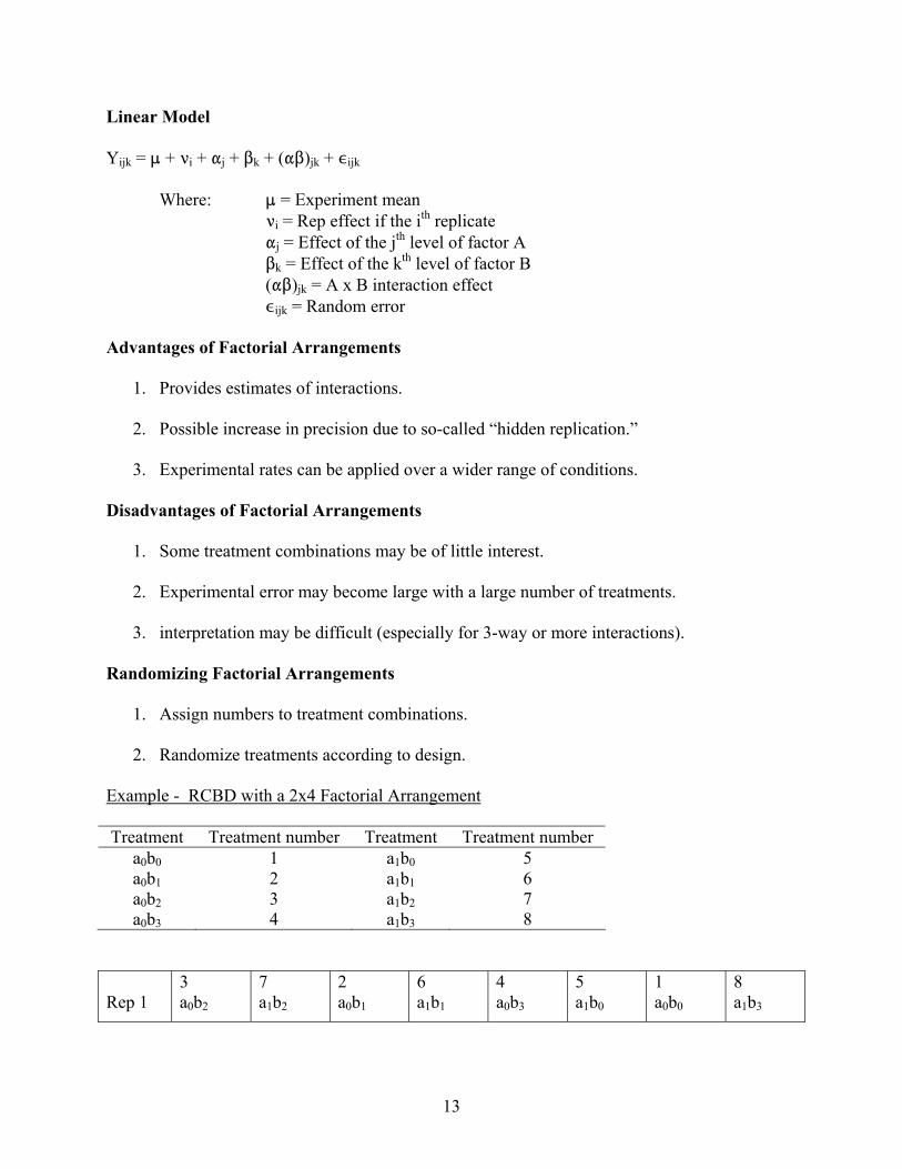
Linear Model Yijk = : + <i + "j + $k + ("$)jk + ,ijk

Where: : = Experiment mean <i = Rep effect if the ith replicate

"j = Effect of the jth level of factor A $k = Effect of the kth level of factor B ("$)jk = A x B interaction effect ,ijk = Random error

Advantages of Factorial Arrangements

1. Provides estimates of interactions. 2. Possible increase in precision due to so-called “hidden replication.”

3. Experimental rates can be applied over a wider range of conditions.

Disadvantages of Factorial Arrangements

1. Some treatment combinations may be of little interest. 2. Experimental error may become large with a large number of treatments.

3. interpretation may be difficult (especially for 3-way or more interactions).

Randomizing Factorial Arrangements

1. Assign numbers to treatment combinations. 2. Randomize treatments according to design.

Example - RCBD with a 2x4 Factorial Arrangement Treatment Treatment number Treatment Treatment number

a0b0 1 a1b0 5 a0b1 2 a1b1 6 a0b2 3 a1b2 7 a0b3 4 a1b3 8

Rep 1

3 a0b2

7 a1b2

2 a0b1

6 a1b1

4 a0b3

5 a1b0

1 a0b0

8 a1b3

13

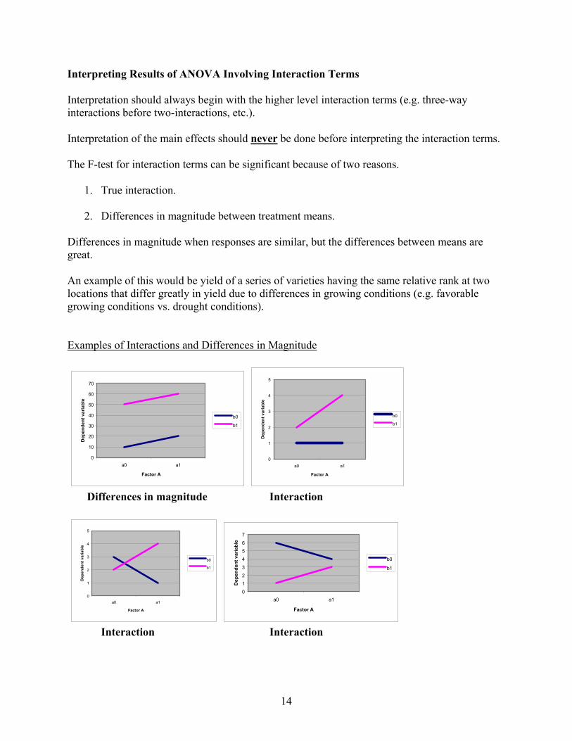
Interpreting Results of ANOVA Involving Interaction Terms Interpretation should always begin with the higher level interaction terms (e.g. three-way interactions before two-interactions, etc.). Interpretation of the main effects should never be done before interpreting the interaction terms. The F-test for interaction terms can be significant because of two reasons.

1. True interaction. 2. Differences in magnitude between treatment means.

Differences in magnitude when responses are similar, but the differences between means are great. An example of this would be yield of a series of varieties having the same relative rank at two locations that differ greatly in yield due to differences in growing conditions (e.g. favorable growing conditions vs. drought conditions). Examples of Interactions and Differences in Magnitude

0

10

20

30

40

50

60

70

a0 a1

Factor A

Dep

ende

nt v

aria

ble

b0

b1

0

1

2

3

4

5

a0 a1

Factor A

Dep

ende

nt v

aria

ble

b0

b1

Differences in magnitude Interaction

0

1

2

3

4

5

a0 a1

Factor A

Dep

ende

nt v

aria

ble

b0

b1

01234567

a0 a1

Factor A

Dep

ende

nt v

aria

ble

b0

b1

Interaction Interaction

14

Flow Chart for Interpreting ANOVA’s with Interaction Terms

Mention that the interaction was NS and discuss the main effects.

Determine why the interaction was significant.

Significant due to a “true” interaction.

Significant due to differences in magnitude.

Significant interaction Non-significant interaction

State that the interaction is significant due tdifferences in magnitude and discuss the main effects. Discussion of the interaction should be avoided.

o Discuss the interaction. Discussion of the main effects should be avoided.

15