plug-in - city university of new yorkuserhome.brooklyn.cuny.edu/irudowsky/mis/plugin/plugint...works...

T3-2 Plug-In T3 Problem Solving Using Excel*

P L U G - I N

T3 Problem Solving Using Excel

1. Describe how to create and sort a list using Excel.2. Explain why you would use conditional formatting using Excel.3. Describe the use of AutoFilter using Excel.4. Explain how to use the Subtotal command using Excel.5. Describe the use of a PivotTable using Excel.

IntroductionIf you routinely track large amounts of information, such as customer mailing lists,phone lists, product inventories, sales transactions, and so on, you can use the ex-tensive list-management capabilities of Excel to make your job easier.

In this plug-in you will learn how to create a list in a workbook, sort the list basedon one or more fields, locate important records by using filters, organize and ana-lyze entries by using subtotals, and create summary information by using pivot ta-bles and pivot charts. The lists that you create will be compatible with Access, and,if you are not already familiar with Access, the techniques that you learn here willgive you a head start on learning several database commands and terms. Plug-InT6, “Basic Skills and Tools Using Access,” will provide detail on many of the Accessdatabase commands and terms.

There are five areas in this plug-in:

1. Lists

2. Conditional Formatting

3. AutoFilter

4. Subtotals

5. PivotTables

ListsA list is a collection of rows and columns of consistently formatted data adher-ing to somewhat stricter rules than an ordinary worksheet. To build a list that

LEARNING OUTCOMES

haa23684_PlugInT3.qxd 9/6/06 5:26 PM Page 2CONFIRMING PAGES

works with all of Excel’s list-management commands, you need to follow a fewguidelines.

When you create a list, keep the following in mind:

� Maintain a fixed number of columns (or categories) of information; you can alter thenumber of rows as you add, delete, or rearrange records to keep your list up to date.

� Use each column to hold the same type of information.

� Don’t leave blank rows or columns in the list area; you can leave blank cells, ifnecessary.

� Make your list the only information in the worksheet so that Excel can more eas-ily recognize the data as a list.

� Maintain your data’s integrity by entering identical information consistently. Forexample, don’t enter an expense category as Ad in one row, Adv in another, andAdvertising in a third if all belong to the same classification.

To create a list in Excel, you would follow these steps:

1. Open a new workbook or a new sheet in an existing workbook.

2. Create a column heading for each field in the list, format the headings in boldtype, and adjust their alignment.

3. Format the cells below the column headings for the data that you plan to use.This can include number formats (such as currency or date), alignment, or anyother formats.

4. Add new records (your data) below the column headings, taking care to be con-sistent in your use of words and titles so that you can organize related recordsinto groups later. Enter as many rows as you need, making sure that there are noempty rows in your list, not even between the column headings and the firstrecord. See Figure T3.1 for a sample list.

Plug-In T3 Problem Solving Using Excel T3-3*

*FIGURE T3.1

An Excel List

Each rowrepresentsa record inthe list.

Each column represents a fieldcontaining one type of information.


SORTING ROWS AND COLUMNS

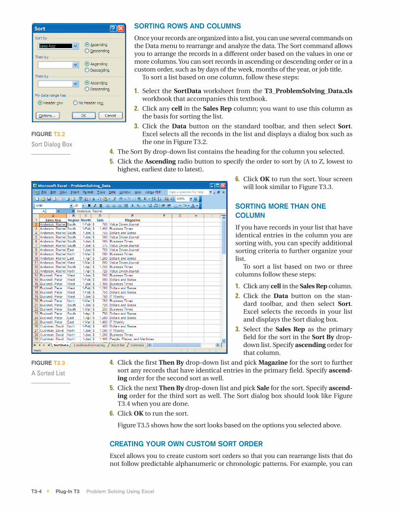
Once your records are organized into a list, you can use several commands onthe Data menu to rearrange and analyze the data. The Sort command allowsyou to arrange the records in a different order based on the values in one ormore columns. You can sort records in ascending or descending order or in acustom order, such as by days of the week, months of the year, or job title.

To sort a list based on one column, follow these steps:

1. Select the SortData worksheet from the T3_ProblemSolving_Data.xlsworkbook that accompanies this textbook.

2. Click any cell in the Sales Rep column; you want to use this column asthe basis for sorting the list.

3. Click the Data button on the standard toolbar, and then select Sort.Excel selects all the records in the list and displays a dialog box such asthe one in Figure T3.2.

4. The Sort By drop-down list contains the heading for the column you selected.

5. Click the Ascending radio button to specify the order to sort by (A to Z, lowest tohighest, earliest date to latest).

6. Click OK to run the sort. Your screenwill look similar to Figure T3.3.

SORTING MORE THAN ONECOLUMN

If you have records in your list that haveidentical entries in the column you aresorting with, you can specify additionalsorting criteria to further organize yourlist.

To sort a list based on two or threecolumns follow these steps:

1. Click any cell in the Sales Rep column.

2. Click the Data button on the stan-dard toolbar, and then select Sort.Excel selects the records in your listand displays the Sort dialog box.

3. Select the Sales Rep as the primaryfield for the sort in the Sort By drop-down list. Specify ascending order forthat column.

4. Click the first Then By drop-down list and pick Magazine for the sort to furthersort any records that have identical entries in the primary field. Specify ascend-ing order for the second sort as well.

5. Click the next Then By drop-down list and pick Sale for the sort. Specify ascend-ing order for the third sort as well. The Sort dialog box should look like FigureT3.4 when you are done.

6. Click OK to run the sort.

Figure T3.5 shows how the sort looks based on the options you selected above.

CREATING YOUR OWN CUSTOM SORT ORDER

Excel allows you to create custom sort orders so that you can rearrange lists that donot follow predictable alphanumeric or chronologic patterns. For example, you can


FIGURE T3.2

Sort Dialog Box

FIGURE T3.3

A Sorted List


create a custom sort order for the regions of the country (West, North, East, South).When you define a custom sort order, it appears in the Options dialog box and isavailable to all the workbooks on your computer.

To create a custom sort order, follow these steps:

1. Choose Tools, Options, and then click the Custom Lists tab.

2. Click the line NEW LIST under Custom Lists section and the text pointer appearsin the List Entries list box. This is where you will type the items in your custom list.

3. Type West, North, South, East, and then click Add. You can either separate eachvalue with a comma or type each one on a separate line. The new custom order ap-pears in the Custom Lists list box, as shown in Figure T3.6.

4. Click OK to close the Options dialog box.

To use a custom sort order, follow these steps:

1. Click any cell in your list.

2. Choose Data, Sort. Excel selects the records in yourlist and displays the Sort dialog box.

3. Select the Region field, and click on Ascendingorder. You may have to remove any secondary andternary sort criteria under the Then By sections.

4. Click Options to display the Sort Options dialog box,as shown in Figure T3.7.

5. Click the First Key Sort Order drop-down list, andclick the custom order you created in the step above.

6. Click OK to run the sort. Your list appears sortedwith the custom criteria you specified.

Creating Conditional FormattingExcel gives you the ability to add conditional formatting—formatting that automat-ically adjusts depending on the contents of cells—to your worksheet. This means


FIGURE T3.4

Sort Dialog Box withMultiple Records

FIGURE T3.5

Data Sort Using MoreThan One Column

FIGURE T3.6

Creating a Custom Sort Order


you can highlight important trends in your data, such as the rise in a stockprice, a missed milestone, or a sudden spurt in your college expenses,based on conditions you set in advance using the Conditional Formattingdialog box. With this feature, an out-of-the-ordinary number jumps out atanyone who routinely uses the worksheet.

For example, if a stock in a Gain/Loss column rises by more than 20 per-cent, you want to display numbers in bold type on a light blue background.In addition, if a stock in the Gain/Loss column falls by more than 20 per-cent, the number will be displayed in bold type on a solid red background.This is where you want to use conditional formatting.

To create such a conditional format, complete the following steps:

1. If the workbook T3_ProblemSolving_Data.xls isclosed, open it.

2. Select the worksheet ConditionalFormatting.

3. Select the column Sale. (Note that each cell canmaintain its own, unique conditional formatting, sothat you can set up several different conditions.)

4. Choose Format, Conditional Formatting. The Con-ditional Formatting dialog box appears, containingseveral drop-down list boxes.

5. In the first list box, select Cell Value Is.

6. In the second list box, select Between.

7. In the first text box, type the number 1000.

8. In the second text box, type the number 1200.

9. Click the Format button and selected Bold style on the Fonts tab and LightBlue on the Patterns tab and then click OK. The formatting will be used forthe cells if the conditional statement you specified in steps 5 through 8 be-comes true.

10. Click the Add button in the Conditional Formatting dialog box to add anoth-er condition to the scenario. The dialog box expands to accept an additional

condition. The Add button lets youadd up to three conditions. The Deletebutton removes conditions you nolonger want.

11. Specify Greater Than as the opera-tor you want to use in the seconddrop-down list box, and then type1250 in the third list box.

12. Click the Format button for Condi-tion 2 and select Bold for the fontstyle on the Font tab, and then,using the Patterns tab, select redshading. Click OK. Figure T3.8 dis-plays the settings for this example.

13. Click OK to close the dialog box,and the conditional formatting willbe applied to the selected text. Ifany numbers fall into the rangesyou specified, the formatting youspecified will be applied. FigureT3.9 shows the conditional format-ting you entered for this example.


FIGURE T3.9

Conditional Formatting

FIGURE T3.8

Conditional FormattingDialog Box

FIGURE T3.7

Sort Options Dialog Box


Using AutoFilter to Find RecordsWhen you want to hide all the records (rows) in your list except those that meet cer-tain criteria, you can use the AutoFilter command on the Filter submenu of theData menu. The AutoFilter command places a drop-down list at the top of each col-umn in your list (in the heading row). To display a particular group of records, selectthe criteria that you want in one or more of the drop-down lists. For example, todisplay the sales history for all employees that had $1,000 orders in January, youcould select January in the Month column drop-down list and $1,000 in the Saledrop-down list.

To use the AutoFilter command to find records, follow these steps:

1. If the workbook T3_ProblemSolving_Data.xls is closed, open it.

2. Select the worksheet AutoFilter.

3. Click any cell in the list.

4. Choose Data, Filter, and then choose AutoFilter from the submenu. Each col-umn head now displays a down arrow.

5. Click the down arrow next to the Region heading. A list box that contains filteroptions appears, as shown in Figure T3.10.

If a column in your list contains one or more blank cells, you will also see (Blanks)and (NonBlanks) options at the bottom of the list. The (Blanks) option displays onlythe records containing an empty cell (blank field) in the filter column, so that you canlocate any missing items quickly. The (NonBlanks) option displays the opposite—allrecords that have an entry in the filter column.

6. Click East to use for this filter. Excel hides the entries that don’t match the crite-rion you specified and highlights the active filter arrow. Figure T3.11 shows theresults of using East as the criterion in the Region column.

You can use more than one filter arrow to further narrow your list, which is useful ifyour list is many records long. To continue working with AutoFilter but to also redisplayall your records, choose Data, Filter, Show All. Excel displays all your records again. To


FIGURE T3.10

AutoFilter Options

Autofilteroptions forthe regioncolumn


remove the AutoFilter drop-down lists, unselect the AutoFilter command on the Filtersubmenu.

CREATING A CUSTOM AUTOFILTER

When you want to display a numeric range of data or customize a column filter inother ways, choose Custom from the AutoFilter drop-down list to display the Cus-tom AutoFilter dialog box. The dialog box contains two relational list boxes and twovalue list boxes that you can use to build a custom range for the filter. For example,you could display all sales greater than $1,000 or all sales between $500 and $800.

To create a custom AutoFilter, follow these steps:

1. Click any cell in the list.

2. If AutoFilter is not already enabled, choose Data, Filter, and then choose AutoFilterfrom the submenu.

3. Click the arrow next to the heading Sale and select (Custom...) from the list ofchoices. The Custom AutoFilter dialog box opens.

4. Click the first relational operator list box and selectis greater than or equal to and then click the valuelist box and select $500.

5. Click the And radio button to indicate that therecords must meet both criteria, then specify is lessthan or equal to in the second relational operatorlist box and select $800 in the second value list box.Figure T3.12 shows the Custom AutoFilter dialogbox with two range criteria specified.

6. Click OK to apply the custom AutoFilter. Therecords selected by the filter are displayed in yourworksheet.


FIGURE T3.12

Custom AutoFilter

Active filterarrow in blue.

Rows that fitthe filtercriteria.

FIGURE T3.11

AutoFilter Output


Analyzing a List with the SubtotalsCommandThe Subtotals command on the Data menu helps you organize and analyze alist by displaying records in groups and inserting summary information,such as subtotals, averages, maximum values, or minimum values. TheSubtotals command can also display a grand total at the top or bottom ofyour list, letting you quickly add up columns of numbers. As a bonus, Subto-tals displays your list in Outline view so that you can expand or shrink eachsection in the list simply by clicking.

To add subtotals to a list, follow these steps:

1. If the workbook T3_ProblemSolving_Data.xls is closed, open it.

2. Select the worksheet Subtotals.

3. Arrange the list so that the records for each group are located together. To do this,sort the list by Region.

4. Choose Data, then select Subtotals. Excel opens the Subtotal dialog box and se-lects the list.

5. In the At Each Change In list box, choose Sales Rep. Each time this valuechanges, Excel inserts a row and computes a subtotal for the numeric fields inthis group of records.

6. In the Use Function list box, choose SUM.

7. In the Add Subtotal To list box, choose Sale, which is the column to use in thesubtotal calculation. Figure T3.13 shows the settings for this example.

8. Click OK to add the subtotals to the list. You will see a screen similar to the one inFigure T3.14, complete with subtotals, outlining, and a grand total.

When you use the Subtotals command in Excel to create outlines, you can exam-ine different parts of a list by clicking buttons in the left margin. Click the numbersat the top of the left margin to choose how many levels of data you want to see.Click the plus or minus button to expand or collapse specific subgroups of data.


FIGURE T3.13

Subtotal Settings

FIGURE T3.14

Subtotals, Outline, and Grand Total

Total forRachel

Anderson

Total forPeter Bucknell


You can choose the Subtotals command as often as necessary to modify yourgroupings or calculations. When you are finished using the Subtotals command,click Remove All in the Subtotal dialog box.

PivotTablesA powerful built-in data-analysis feature in Excel is the PivotTable. A PivotTable an-alyzes, summarizes, and manipulates data in large lists, databases, worksheets, orother collections. It is called a PivotTable because fields can be moved within thetable to create different types of summary lists, providing a “pivot.” PivotTablesoffer flexible and intuitive analysis of data.

Although the data that appear in PivotTables look like any other worksheet data,the data in the data area of the PivotTable cannot be directly entered or changed.The PivotTable is linked to the source data; the output in the cells of the table areread-only data. The formatting (number, alignment, font, etc.) can be changed aswell as a variety of computational options such as SUM, AVERAGE, MIN, and MAX.

PIVOTTABLE TERMINOLOGY

Some notable PivotTable terms are:

� Row field—Row fields have a row orientation in a PivotTable report and are dis-played as row labels. These appear in the ROW area of a PivotTable report layout.

� Column field—Column fields have a column orientation in a PivotTable reportand are displayed as column labels. These appear in the COLUMN area of a Piv-otTable report layout.

� Data field—Data fields from a list or table contain summary data in a PivotTable,such as numeric data (e.g., statistics, sales amounts). These are summarized inthe DATA area of a PivotTable report layout.

� Page field—Page fields filter out the data for other items and display one page ata time in a PivotTable report.

BUILDING A PIVOTTABLE

The PivotTable wizard steps through the process of creating a PivotTable, allowinga visual breakdown of the data in the Excel list or database. When the wizard stepsare complete, a diagram, such as Figure T3.15, with the labels PAGE, COLUMN,


FIGURE T3.15

The PivotTable, PivotTableToolbar, and PivotTableField List

ROWFields

COLUMNFields

PAGEFields

DATA ITEMS


ROW, and DATA appears. The next step is to drag thefield buttons onto the PivotTable grid. This step tellsExcel about the data needed to be analyzed with a Piv-otTable.

Using the PivotTable Feature

1. If the workbook T3_ProblemSolving_Data.xls isclosed, open it.

2. Select the worksheet PivotTableData. Click anycell in the list. Now the active cell is within the list,and Excel knows to use the data in the Excel list tocreate a PivotTable.

3. Select Data on the menu bar, then choose Pivot-Table and PivotChart Report. The PivotTable andPivot Chart Wizard—Step 1 of 3 dialog box opens, as shown in Figure T3.16.

4. In the Where is the data that you want to analyze? area, choose MicrosoftExcel list or database if it is not already selected.

5. In the What kind of report do you want to create? area, choose PivotTable.

6. Click the Next button. The PivotTable and PivotChart Wizard—Step 2 of 3 dia-log box opens. In the Range box, the range should be $A$1:$E$97, which de-fines the data range to use for the PivotTable. The range must include thecolumn headings in row 1, which will be the names of the fields to drag into thePivotTable.

7. Click the Next button. The PivotTable and PivotChart Wizard—Step 3 of 3 dia-log box opens. This dialog box is used to tell Excel whether to place the Pivot-Table on an existing or new worksheet. Select New Worksheet.

8. The next step is to design the layout of the PivotTable. Click the Layout button.Excel opens the PivotTable and PivotChart Wizard–Layout dialog box, as shownin Figure T3.17.

9. The fields appear on buttons to the right in the dialog box. These currently arethe column fields. The four areas you can define to create your PivotTable areROW, COLUMN, DATA, and PAGE.

10. In the next step, you will drag the field buttons to the areas to define the layout of thePivotTable. For example, to summarize the values in a field in the body of the table,place the field button in the DATA area. To arrange items in a field in columns withthe labels across the top, place the field button in the COLUMN area. To arrangeitems in a field of rows with labels along the side, place the field button in the ROW


FIGURE T3.16

The PivotTable andPivotChart Wizard—Step 1of 3 Dialog Box

FIGURE T3.17

The PivotTable andPivotChart Wizard—Layout Dialog Box


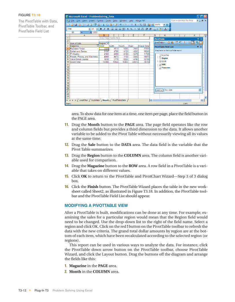
area. To show data for one item at a time, one item per page, place the field button inthe PAGE area.

11. Drag the Month button to the PAGE area. The page field operates like the rowand column fields but provides a third dimension to the data. It allows anothervariable to be added to the Pivot Table without necessarily viewing all its valuesat the same time.

12. Drag the Sale button to the DATA area. The data field is the variable that thePivot Table summarizes.

13. Drag the Region button to the COLUMN area. The column field is another vari-able used for comparison.

14. Drag the Magazine button to the ROW area. A row field in a PivotTable is a vari-able that takes on different values.

15. Click OK to return to the PivotTable and PivotChart Wizard—Step 3 of 3 dialogbox.

16. Click the Finish button. The PivotTable Wizard places the table in the new work-sheet called Sheet2, as illustrated in Figure T3.18. In addition, the PivotTable tool-bar and the PivotTable Field List should appear.

MODIFYING A PIVOTTABLE VIEW

After a PivotTable is built, modifications can be done at any time. For example, ex-amining the sales for a particular region would mean that the Region field wouldneed to be changed. Use the drop-down list to the right of the field name. Select aregion and click OK. Click on the red ! button on the PivotTable toolbar to refresh thedata with the new criteria. The grand total dollar amounts by region are at the bot-tom of each item, which have been recalculated according to the selected region (orregions).

This report can be used in various ways to analyze the data. For instance, clickthe PivotTable down arrow button on the PivotTable toolbar, choose PivotTableWizard, and click the Layout button. Drag the buttons off the diagram and arrangethe fields like this:

1. Magazine in the PAGE area.

2. Month in the COLUMN area.


FIGURE T3.18

The PivotTable with Data,PivotTable Toolbar, andPivotTable Field List


3. Sale in the DATA area.

4. Sales Rep in the ROW area.

The completed PivotTable dialog box should look like the one in Figure T3.19.The PivotTable now illustrates the sales by month for each salesperson, along withthe total amount for the sales for each sales representative.

PIVOTTABLE TOOLSThere are a number of PivotTable tools that you should be aware of, such as:

� PivotTable—Contains commands for working with a PivotTable.

� Format Report—Enables the user to format the PivotTable report.

� Chart Wizard—Enables the user to create a chart using the data in the PivotTable.

� Hide Detail—Hides the detail information in a PivotTable and shows only thetotals.

� Show Detail—Shows the detail information in a PivotTable.

� Refresh External Data—Allows the user to refresh the data in the PivotTableafter changes to data are made in the data source.

� Include Hidden Items in Totals—Lets the user show the hidden items in the totals.

� Always Display Items—Always shows the field item buttons with drop-downarrows in the PivotTable.

� Field Settings—Displays the PivotTable Field dialog box so that the user canchange computations and their number format.

� Hide Field List—Hides and shows the PivotTable Field List window.

BUILDING A PIVOTCHART

A PivotChart is a column chart (by default) that is based on the data in a PivotTable.The chart type can be changed if desired. To build a PivotChart:

1. Click the Chart Wizard (see Figure T3.20) on the PivotTable toolbar. Excel willautomatically create a new worksheet, labeled Chart 1, and display the currentPivotTable information in chart form like Figure T3.21.


FIGURE T3.19

Rearranged Data in thePivotTable


FIGURE T3.21

PivotChart

FIGURE T3.20

PivotTable Toolbar

2. Modifications to the PivotChart can be done by selecting the drop-down lists tothe right of the field names.

Note: Whatever changes are selected on the PivotChart are also made to the Pivot-Table, as the two features are linked dynamically.



P L U G - I N S U M M A R Y*

M A K I N G B U S I N E S S D E C I S I O N S*


If you routinely track large amounts of information, you can use several Excel tools forproblem solving. A list is a table of data stored in a worksheet, organized into columns offields and rows of records. Excel gives you the ability to add conditional formatting—

formatting that automatically adjusts depending on the contents of cells—to your worksheet.The AutoFilter command places a drop-down list at the top of each column in your list (in theheading row). The Subtotals command on the Data menu helps you organize and analyze a listby displaying records in groups and inserting summary information, such as subtotals, aver-ages, maximum values, or minimum values. A PivotTable analyzes, summarizes, and manipu-lates data in large lists, databases, worksheets, or other collections.

1. Production ErrorsEstablished in 2002, t-shirts.com has rapidly become the place to find, order, and save on T-shirts. One huge selling factor is that the company manufactures its own T-shirts. However,the quality manager for the production plant, Kasey Harnish, has noticed an unacceptablenumber of defective T-shirts being produced. You have been hired to assist Kasey in under-standing where the problems are concentrated. He suggests using a PivotTable to performan analysis and has provided you with a data file, T3_TshirtProduction_Data.xls. The fol-lowing is a brief definition of the information within the data file:

A. Batch: A unique number that identifies each batch or group of products produced.B. Product: A unique number that identifies each product.C. Machine: A unique number that identifies each machine on which products are produced.D. Employee: A unique number that identifies each employee producing products.E. Batch Size: The number of products produced in a given batch.F. Num Defect: The number of defective products produced in a given batch.

2. Coffee TrendsCollege chums Hannah Baltzan and Tyler Phillips are working on opening a third espressodrive-through stand in Highlands Ranch, Colorado, called Brewed Awakening. Their origi-nal drive-through stand, Jitters, and their second espresso stand, Bean Scene, have donewell in their current locations in Englewood, Colorado, five miles away. Since Hannah andTyler want to start with low overhead, they need assistance analyzing the data from thepast year on the different types of coffee and amounts that they sold from both stands.Hannah and Tyler would like a recommendation of the four top sellers to start offeringwhen Brewed Awakening opens. They have provided you with the data file T3_Jitter-sCoffee_Data.xls for you to perform the analysis that will support your recommendation.

3. Filtering SecureIT DataSecureIT, Inc., is a small computer security contractor that provides computer securityanalysis, design, and software implementation for commercial clients. Almost all of Se-cureIT work requires access to classified material or company confidential documents.Consequently, all of the security personnel have clearances of either Secret or Top Secret.



Some have even higher clearances for work that involves so-called black box securitywork.

While most of the personnel information for SecureIT resides in database systems, abasic employee worksheet is maintained for quick calculations and ad hoc report genera-tion. Because SecureIT is a small company, it can take advantage of Excel’s excellent listmanagement facilities to satisfy many of its personnel information management needs. Youhave been provided with a sample worksheet, T3_Employee_Data.xls, to assist SecureITwith producing several worksheet summaries. Here is what is needed:

1. One worksheet that is sorted by last name and hire data.2. One worksheet that uses a custom sort by department in this order: Marketing, Human

Resources, Management, and Engineering.3. One worksheet that uses a filter to display only those employees in the Engineering

department with a clearance of Top Secret (TS).4. One worksheet that uses a custom filter to display only those employees born between

1960 and 1969 (inclusive).5. One worksheet that totals the salaries by department and the grand total of all depart-

ment salaries. This worksheet should be sorted by department name first.

4. Filtering RedRocks Consulting ContributionsRedRocks Consulting is a large computer consulting firm in Denver, Colorado. Don McCub-brey, the CEO and founder of the firm, is well-known for his philanthropic efforts. He believesthat many of his employees also contribute to nonprofit organizations and wants to rewardthem for their efforts while encouraging others to contribute to charities. He started a pro-gram in which RedRocks Consulting matches 50 percent of each donation an employeemakes to the charity of his or her choice. The only guidelines are that the charity must be anonprofit organization and the firm’s donation per employee may not exceed $500 a year.

Don has started an Excel file, T3_RedRocks_Data.xls, to record the firm’s donations. In-cluded in this file are the dates the request for a donation was submitted, the employee’sname and ID number, the name of the charity, the dollar amount contributed by the firm,and the date the contribution was sent. Don wants you to help him create several work-sheets with the following criteria:

1. One worksheet that sorts the list alphabetically by organization and then by employee’slast name.

2. One worksheet that totals the contribution made per employee for the month of De-cember.

3. One worksheet that sorts the list by donation value by lowest amount to highestamount.


plug-in - city university of new yorkuserhome.brooklyn.cuny.edu/irudowsky/mis/plugin/plugint...works...

Documents