plugpower tp - final - march 2003.doc | us epa archive ... · table 3-1 verification parameter dqos...
TRANSCRIPT


SRI/USEPA-GHG-QAP-25 March 2003
Test and Quality Assurance Plan Residential Electric Power Generation Using the Plug Power SU1 Fuel Cell System
Prepared by:
Greenhouse Gas Technology Center Southern Research Institute
Under a Cooperative Agreement With U.S. Environmental Protection Agency
and
Under Agreement With New York State Energy Research and Development Authority

EPA REVIEW NOTICE
This report has been peer and administratively reviewed by the U.S. Environmental Protection Agency, and approved for publication. Mention of trade names or commercial products does not constitute endorsement or recommendation for use.

SRI/USEPA-GHG-QAP-25 February 2003
Greenhouse Gas Technology Center A U.S. EPA Sponsored Environmental Technology Verification ( ) Organization
Test and Quality Assurance Plan
Residential Electric Power Generation Using the Plug Power SU1 Fuel Cell System
Prepared by: Greenhouse Gas Technology Center
Southern Research Institute PO Box 13825
Research Triangle Park, NC 27709 USA Telephone: 919/806-3456
Reviewed by: New York State Energy Research and Development Authority
Plug Power . U.S. EPA Office of Research and Development QA Team
indicates comments are integrated into Test Plan

(this page intentionally left blank)

Greenhouse Gas Technology Center A U.S. EPA Sponsored Environmental Technology Verification ( ) Organization
Test and Quality Assurance Plan
Residential Electric Power Generation Using the Plug Power SU1 Fuel Cell System
This Test and Quality Assurance Plan has been reviewed and approved by the Greenhouse Gas Technology Center Project Manager and Director, the U.S. EPA APPCD Project Officer, and the U.S. EPA APPCD Quality Assurance Manager.
Stephen Piccot Date David Kirchgessner Date Director APPCD Project Officer Greenhouse Gas Technology Center U.S. EPA Southern Research Institute
William Chatterton Project Manager Greenhouse Gas Technology Center Southern Research Institute
Date Shirley Wasson Date APPCD Quality Assurance Manager
U.S. EPA
Test Plan Final: April 2003

(this page intentionally left blank)

SRI/USEPA-GHG-QAP-25 March 2003
TABLE OF CONTENTS Page
Appendices ................................................................................................................................................iii List of Figures ................................................................................................................................................iii List of Tables ................................................................................................................................................iii Distribution List ................................................................................................................................................iv
1.0 INTRODUCTION .................................................................................................................................1-11.1 BACKGROUND ..........................................................................................................................1-11.2 TEST FACILITY DESCRIPTION ...............................................................................................1-31.3 PEM FUEL CELL TECHNOLOGY DESCRIPTION .................................................................1-51.4 PERFORMANCE VERIFICATION PARAMETERS .................................................................1-7
1.4.1 Power Production Performance .......................................................................................1-91.4.2 Power Quality Performance ...........................................................................................1-101.4.3 Air Pollutant Emission Performance..............................................................................1-101.4.4 Emission Reductions......................................................................................................1-10
1.5 ORGANIZATION ......................................................................................................................1-111.6 SCHEDULE................................................................................................................................1-12
2.0 VERIFICATION APPROACH............................................................................................................2-12.1 OVERVIEW .................................................................................................................................2-12.2 POWER PRODUCTION PERFORMANCE ...............................................................................2-2
2.2.1 Electrical Power Output and Efficiency...........................................................................2-32.2.1.1 ION Electrical Power Meter.............................................................................2-72.2.1.2 Battery Voltage and Current Sensors ...............................................................2-72.2.1.3 Fuel Gas Meter .................................................................................................2-72.2.1.4 Gas Temperature and Pressure Measurements .................................................2-82.2.1.5 Gas Composition and Heating Value Analysis ................................................2-82.2.1.6 Ambient Conditions Measurements .................................................................2-9
2.3 POWER QUALITY PERFORMANCE .......................................................................................2-92.3.1 Electrical Frequency ......................................................................................................2-102.3.2 Generator Line Voltage..................................................................................................2-102.3.3 Voltage Total Harmonic Distortion ...............................................................................2-112.3.4 Current Total Harmonic Distortion................................................................................2-122.3.5 Power Factor ..................................................................................................................2-122.3.6 Power Quality Measurement Instruments ......................................................................2-12
2.4 FUEL CELL EMISSIONS..........................................................................................................2-122.4.1 Reference Method Modifications...................................................................................2-142.4.2 Temporary Test Duct, Gaseous Sample Conditioning and Handling ............................2-152.4.3 Gaseous Pollutant Analytical Procedures ......................................................................2-172.4.4 Determination of Emission Rates...................................................................................2-18
2.5 ELECTRICITY OFFSETS AND ESTIMATION OF EMISSION REDUCTIONS ..................2-202.5.1 Estimated Annual Emission Reductions for the Lewiston Residence ...........................2-20
3.0 DATA QUALITY ..................................................................................................................................3-13.1 BACKGROUND ..........................................................................................................................3-13.2 ELECTRICAL POWER OUTPUT AND POWER QUALITY ...................................................3-13.3 EFFICIENCY................................................................................................................................3-2
3.3.1 Natural Gas and Fuel Flow Rate Quality Assurance .......................................................3-63.3.2 Gas Pressure and Barometric Pressure Quality Assurance ..............................................3-7
i

SRI/USEPA-GHG-QAP-25 March 2003
3.3.3 Gas Temperature and Ambient Temperature Quality Assurance ....................................3-73.3.4 Fuel Gas Analyses Quality Assurance .............................................................................3-7
3.4 EMISSIONS TESTING QA/QC PROCEDURES........................................................................3-93.4.1 Analyzer and Sampling System QA/QC Procedures .....................................................3-113.4.2 NOX Sampling System Bias Test and Exhaust Flow Rate Verification
(Standard Addition Procedure) ......................................................................................3-143.4.2.1 NOX Sampling System Bias Test ...................................................................3-143.4.2.2 Exhaust Gas Flow Rate Verification ..............................................................3-16
3.5 INSTRUMENT TESTING, INSPECTION, AND MAINTENANCE .......................................3-173.6 INSPECTION/ACCEPTANCE OF SUPPLIES AND CONSUMABLES.................................3-17
4.0 DATA ACQUISITION, VALIDATION, AND REPORTING..........................................................4-14.1 DATA ACQUISITION AND STORAGE....................................................................................4-1
4.1.1 Continuous Measurements Data Acquisition...................................................................4-14.1.2 Emission Measurements ..................................................................................................4-44.1.3 Fuel Gas Sampling ...........................................................................................................4-4
4.2 DATA REVIEW, VALIDATION, AND VERIFICATION.........................................................4-44.3 RECONCILIATION OF DATA QUALITY OBJECTIVES........................................................4-54.4 ASSESSMENTS AND RESPONSE ACTIONS ..........................................................................4-5
4.4.1 Project Reviews ...............................................................................................................4-64.4.2 Inspections .......................................................................................................................4-64.4.3 Performance Evaluation Audit.........................................................................................4-64.4.4 Technical Systems Audit .................................................................................................4-74.4.5 Audit of Data Quality.......................................................................................................4-7
4.5 DOCUMENTATION AND REPORTS .......................................................................................4-74.5.1 Field Test Documentation ................................................................................................4-74.5.2 QC Documentation ..........................................................................................................4-84.5.3 Corrective Action and Assessment Reports .....................................................................4-84.5.4 Verification Report and Verification Statement ..............................................................4-8
4.6 TRAINING AND QUALIFICATIONS .......................................................................................4-94.7 HEALTH AND SAFETY REQUIREMENTS .............................................................................4-9
5.0 REFERENCES ......................................................................................................................................5-1
ii

SRI/USEPA-GHG-QAP-25 March 2003
APPENDICES Page
Appendix A-1 Test Procedures and Field Log Forms............................................................... A-1
LIST OF FIGURES Page
Host Site in Lewiston, NY ................................................................................ 1-3Figure 1-1. Figure 1-2 Plug Power SU1 System Installed at the Host Site in Lewiston, NY................ 1-3 Figure 1-3 Percentage of Energy Used Per Circuit for August 11, 2002 ............................ 1-4 Figure 1-4 Hourly Peak Power Levels for August 11, 2002 ............................................... 1-5 Figure 1-5 Simple Process Diagram ................................................................................... 1-6 Figure 1-6 Project Organization.......................................................................................... 1-11 Figure 2-1 Schematic of Measurement System .................................................................. 2-2 Figure 2-2 SU1 System Power Output................................................................................ 2-5 Figure 2-3 Gas Sampling and Analysis System .................................................................. 2-15 Figure 3-1 Exhaust Gas Spiking Technique........................................................................ 3-14 Figure 4-1 DAS Schematic ................................................................................................. 4-2
LIST OF TABLES Page
Table 1-1 Plug Power SU1 System Specifications............................................................ 1-8 Table 2-1 Permissible Power, Fuel, and Atmospheric Condition Variations.................... 2-3 Table 2-2 Summary of Emission Testing Methods ......................................................... 2-13 Table 2-3 Modifications to Reference Method Specifications ........................................ 2-16 Table 2-4 Electrical Demand of the Lewiston Residence ............................................... 2-21 Table 2-5 Displaced Emission Rates for the NY ISO (2002).......................................... 2-24 Table 3-1 Verification Parameter DQOs ........................................................................... 3-1 Table 3-2 Measurement Instrument Specifications and DQI Goals .................................. 3-3 Table 3-3 Summary of QA/QC Checks............................................................................. 3-5 Table 3-4 Electrical Efficiency Error Propagation and DQO............................................ 3-6 Table 3-5 ASTM D1945 Repeatability Specifications...................................................... 3-8 Table 3-6 DQIs for Anticipated Component Concentrations ............................................ 3-8 Table 3-7 Instrument Specifications and DQI Goals for Stack Emissions Testing......... 3-10 Table 3-8 Summary of Emissions Testing QC Checks ................................................... 3-11 Table 3-9 Spike Gas Flow Rates for a Given Incremental Change................................. 3-15 Table 3-10 NO2 Delta for Given Spike Gas Flow Rates ................................................... 3-16 Table 4-1 Continuous Data to be Collected for Fuel Cell Evaluation ............................... 4-3
iii

SRI/USEPA-GHG-QAP-25 March 2003
DISTRIBUTION LIST
New York State Energy Research and Development Authority (NYSERDA) Richard Drake James Foster
Plug Power David Rollins
U.S. EPA – Office of Research and Development David Kirchgessner Shirley Wasson
Southern Research Institute (GHG Center) Stephen Piccot Robert Richards
William Chatterton Ashley Williamson
iv

SRI/USEPA-GHG-QAP-25 March 2003
1.0 INTRODUCTION
1.1 BACKGROUND
The U.S. Environmental Protection Agency’s Office of Research and Development (EPA-ORD) operates the Environmental Technology Verification (ETV) program to facilitate the development of innovative technologies through performance verification and information dissemination. The goal of the ETV program is to further environmental protection by substantially accelerating the acceptance and use of improved and innovative environmental technologies. Congress funds ETV in response to the belief that there are many viable environmental technologies that are not being used because of the lack of credible third-party performance data. With performance data developed under this program, technology buyers, financiers, and permitters in the United States and abroad will be better equipped to make informed decisions regarding purchase and use of environmental technologies.
The Greenhouse Gas Technology Center (GHG Center) is one of six verification organizations operating under the ETV program. The GHG Center is managed by EPA’s partner verification organization, Southern Research Institute (SRI), which conducts verification testing of promising GHG mitigation and monitoring technologies. The GHG Center’s verification process consists of developing verification protocols, conducting field tests, collecting and interpreting field and other data, obtaining independent peer-review input, and reporting findings. Performance evaluations are conducted according to externally reviewed verification Test and Quality Assurance Plans ("Test Plans") and established protocols for quality assurance (QA).
The GHG Center is guided by volunteer groups of stakeholders. These stakeholders offer advice on specific technologies most appropriate for testing, help disseminate results, and review the Test Plans and Technology Verification Reports generated and published by the GHG Center at the conclusion of each technology verification. The GHG Center’s Executive Stakeholder Group consists of national and international experts in the areas of climate science and environmental policy, technology, and regulation. It also includes industry trade organizations, environmental technology finance groups, governmental organizations, and other interested groups. The GHG Center’s activities are also guided by industryspecific stakeholders who provide guidance on the verification testing strategy related to their area of expertise and peer-review key documents prepared by the GHG Center.
Distributed electrical power generation is a technology area of interest to some GHG Center stakeholders. Distributed generation (DG) refers to electricity generation equipment, typically ranging in size from 5 to 1,000 kilowatts (kW), that provides electric power at a customer's site (as opposed to central station generation). A DG unit can be connected directly to the customer and/or to a utility’s transmission and distribution (T&D) system. Examples of technologies available for DG include gas turbine generators, internal combustion (IC) engine generators (gas, diesel, other), photovoltaics, wind turbines, fuel cells, and microturbines. DG technologies provide customers one or more of the following main services: standby generation (i.e., emergency backup power), peak-shaving generation (during high-demand periods), base-load generation (constant generation), or cogeneration (combined heat and power (CHP) generation).
The GHG Center and the New York State Energy Research and Development Authority (NYSERDA) have agreed to collaborate and share the cost of verifying several new DG technologies located throughout the State of New York. One such technology is the Plug Power Stationary Unit 1 Fuel Cell Demonstration System (SU1 System) commercially offered as a technology demonstrator by Plug Power
1-1

SRI/USEPA-GHG-QAP-25 March 2003
of Latham, New York. The SU1 System is a Proton Exchange Membrane (PEM) fuel cell capable of producing 5 kW of electrical power in a residential setting. Using pipeline natural gas available at many residences, the SU1 System contains a reformer that converts natural gas into hydrogen (H2), allowing electricity to be generated by the SU1 System through a relatively low-temperature electrochemical reaction between H2, oxygen (O2), and a solid electrolyte (the proton exchange membrane). Because the reforming process also produces carbon monoxide (CO), a poison to proton exchange membranes, the fuel processor also contains a CO cleanup step to remove CO or transform it into carbon dioxide (CO2). PEM fuel cell capacities generally range between 5 and 250kW, and electrical conversion efficiencies can vary from about 25 to 40 percent.
As part of a research and development partnership between NYSERDA, National Fuel Gas Company (NFG), the Department of Energy (DOE), and others, a fully interconnected SU1 System was installed at a private single-family residence located in Lewiston, New York (Niagara County) for a one-year system integration demonstration. The GHG Center, in partnership with NYSERDA, will conduct a performance verification of the SU1 System installed and operating at the Lewiston site. Field tests will be performed to independently verify the electricity generation rate, electrical power quality, energy efficiency, conventional and criteria air pollutant emissions, and GHG emission reductions from offsetting electricity generation from the utility grid. The overall energy conversion efficiency is estimated to range between 20 to 30 percent which, depending on the mix of energy sources used to supply electricity to the local electrical grid, could reduce greenhouse gas (GHG) emissions.
This document is the Test Plan for performance verification of the Plug Power SU1 System demonstrator. It contains the rationale for the selection of verification parameters, the verification approach, data quality objectives (DQOs), and Quality Assurance/Quality Control (QA/QC) procedures. This Test Plan will guide implementation of the test, creation of the Verification Report and other documentation, and data analysis.
This Test Plan has been reviewed by NYSERDA, NFG, Plug Power, the EPA ETV QA team, and selected members of the GHG Center’s Advanced Energy Stakeholder group. Once approved, it will meet the requirements of the GHG Center’s Quality Management Plan (QMP) and thereby satisfy the ETV QMP requirements, as evidenced by the signature sheet at the front of this document. The final Test Plan will be posted on the Web sites maintained by the GHG Center (www.sri-rtp.com) and the ETV program (www.epa.gov/etv).
The GHG Center will prepare the Verification Report upon field test completion. The Verification Report will include a Verification Statement which will provide an executive summary of the evaluation. The Verification Report and Statement will be reviewed by the same organizations listed above, followed by EPA-ORD technical review. When this review is complete, the GHG Center Director and EPA-ORD Laboratory Director will sign the Report and Statement, and the final documents will be posted on the GHG Center and ETV program Web sites.
The following section provides a description of the SU1 System and Lewiston test site. This is followed by a list of performance verification parameters that will be quantified through independent testing at the site. The section concludes with a discussion of key organizations participating in this verification, their roles, and the verification test schedule. Section 2.0 describes the technical approach for verifying each parameter, including sampling, analytical, and QA/QC procedures. Section 3.0 identifies the data quality assessment criteria for critical measurements and states the accuracy, precision, and completeness goals for each measurement. Section 4.0 discusses data acquisition, validation, reporting, and auditing procedures.
1-2

SRI/USEPA-GHG-QAP-25 March 2003
1.2 TEST FACILITY DESCRIPTION
The Lewiston residence, shown in Figure 1-1, is a typical two-story single family home with a partial basement. The home is located in Niagara County, New York and includes 2,060 ft2 of conventional living space and 700 ft2 of basement space. The home was constructed in the early 1970’s, and contains walls that are insulated at a typical R-11 level and ceilings that are R-19 rated. Figure 1-2 is a photograph of the Plug Power SU1 System which was installed at the residence in April of 2001.
Figure 1-1. Host Site in Lewiston, NY
Figure 1-2. Plug Power SU1 System Installed at the Host Site in Lewiston, NY
1-3

SRI/USEPA-GHG-QAP-25 March 2003
Space heating at the home is provided by a natural gas-fired boiler, which heats water that is circulated through baseboard heat exchangers using two electric circulating pumps. In addition to standard electrical outlets and lighting fixtures throughout the home, it contains a hot tub, electrical washer, and gas dryer (dryer motor is electric), several ceiling fan/light units, a refrigerator, dishwasher, microwave, several television sets, computer, sump pump, freezer, and other miscellaneous electrical devices.
All of the major electric circuits and loads are being continuously monitored as part of the long-term system demonstration being conducted at this home by the DOE and NYSERDA partners (13). Data collected during this demonstration is useful for designing and implementing this performance verification. Figure 1-3 below is an example of the energy use features of the Lewiston home for a typical summer day in 2002. Although in this example the hot tub did not consume significant amounts of electricity, the hot tub can dominate energy use during operation, accounting for well over 50 percent of the total kWh used in a day.
Figure 1-3. Percentage of Energy Used Per Circuit for August 11, 2002
outlets-D 34.1%
hot tub
outlets-A dryer
/0.0%
4.7%
outl
outl5.3%
kit/refrig
kit/din
sump frz5.4%
washer
range
ets-C
7.4%
outlets-B 2.1%
dishwash outlets-C 0.0%
kit/refrig boiler outlets-A 0.0% 0.2% kit/din
hot tub boiler 0.4%
dishwash ets-B 0.7%
dryer
outlets-D
washer
sump/frz
range
39.7%
Figure 1-4 shows peak power consumed at the home for each hour on August 11, 2002. The figure also contains a line graph depicting the fuel cell power output occurring throughout the day. Since the fuel cell was set to deliver 2.5 kW of power, it did not meet the peak demand at the home for roughly two thirds of the day. If the SU1 System were set at its highest power command, 5kW, it would have supplied most of the current needed on August 11, 2002.
1-4

SRI/USEPA-GHG-QAP-25 March 2003
kW (p
eak)
Figure 1-4. Hourly Peak Power Levels for August 11, 2002
8.5
8.0
7.5
7.0
6.5
6.0
5.5
5.0
4.5
4.0
3.5
3.0
2.5
2.0
1.5
1.0
0.5
0.0
hot tub
sump/frz
dryer
dishwash
boiler
kit/refrig
kit/din
outlets-D
outlets-C
outlets-B
outlets-A
Fuel Cell
1.3 PEM FUEL CELL TECHNOLOGY DESCRIPTION
PEM fuel cells generate electricity through a reaction between H2, O2, and a solid electrolyte (the proton exchange membrane). This type of fuel cell operates at relatively low temperatures (about 175 °F) and can vary output fairly quickly to meet changes in demand. The basic principle of operation is to convert H2 into electrical energy with an electrochemical reaction with O2, generally supplied from ambient air. Since H2 fuel is not readily available, fuel cells often employ reformer technologies that convert standard hydrocarbon-based fuels, such as natural gas, into a H2-rich fuel stream that can be used in the fuel cell stack. PEM fuel cell capacities generally range from 5 to 250 kW, with electrical efficiencies from about 25 to 40 percent, depending on manufacturer and installation specifics. Heat recovery equipment can be coupled with PEM fuel cells to significantly increase overall system efficiency, although the SU1 System being verified does not use this technology.
Figure 1-5 is a simplified process flow diagram of the SU1 System. It shows the three main components of the system including: (1) the fuel processor, (2) the fuel cell stack, and (3) the power conditioner, each of which are described below.
010
020
0 30
0 40
050
060
070
0 80
0 90
010
0011
001
0013
015
0016
001
0018
019
0021
002
002
000014
0 0 00202 7 2 3
1-5

SRI/USEPA-GHG-QAP-25 March 2003
1-6
Figure 1-5. Simple Process Diagram
Fuel In
FuelProcessor
CO RemovalSystem
TreatedReformate(H2, CO2)
Raw Reformate(H2, CO, CO2)
Fuel Processor Fuel Cell Stack Power ConditionerNatural Gas Reformed Fuel
Reformed Fuel
Oxidant InputWaste Heat
Water
DC PowerConditionedAC Power
+_
DC Power
-e
Anode Cathode
Membrane
+e
-e
+eH2 In
H20 Out
O2 InLow Voltage DC Power
Auxiliary DCFrom Battery
PowerTransformer
AC PowerOut
Emissions
Because pure H2 is usually not readily available, a reformed fuel (reformate) rich in H2 is derived from fuels such as natural gas, propane, methanol, or other petroleum products using a fuel processor. Typical fuel-processing methods include catalytic steam reforming (CSR), partial oxidation (POX), and auto- thermal reforming (ATR). Each type of reformer requires a heat source and an O2 source to oxidize the fuel. The CSR reforming process yields the highest H2 per unit of fuel, boosting fuel quality and fuel cell efficiency. This occurs because all of the O2 needed to oxidize the carbon compounds is provided by steam, which also contributes to the H2 content of the reformate. In the case of POX reforming, air is used to oxidize the fuel and, therefore, no H2 is contributed by the oxidant. With ATR, both air and steam are used in the process. Air is used to burn just enough fuel to drive the reforming reaction. Steam supplies the O2 to complete the reaction. The SU1 System uses ATR. The reformate created by fuel processing consists primarily of H2, CO2, and CO. The fuel processor also contains a CO cleanup component to remove or transform all or most of the CO to CO2 and minimize CO damage to the system. Most fuel cells incorporate shift reactors and/or selective oxidation reactors to oxidize the CO to CO2. The SU1 System uses a selective oxidation process to limit CO concentrations entering the fuel cell stack by converting it to CO2.

SRI/USEPA-GHG-QAP-25 March 2003
Electricity is generated in the PEM fuel cell stack. The stack consists of a series electrodes (an anode and cathode) separated by an ion-exchange membrane. The size and number of electrodes and membranes assembled in a stack dictates the electrical voltage and power levels produced. The membrane is a fluorinated sulfonic-acid polymer or other organic polymer that allows hydrogen ions (H+) ions to pass through it. Each of the electrodes are coated with a platinum-based catalyst. The reformate is directed into the anode and air enters the system through the cathode during operation. The H2 molecules in the reformate split into two protons and two electrons in the presence of the platinum-based catalyst. The electrons flow through an external circuit creating a low-voltage direct electrical current (DC). The H+
protons pass through the membrane and combine at the cathode with the electrons and O2 from the air to form water and generate waste heat.
PEM fuel cells also include a power conditioner. This component uses an inverter to convert the lowvoltage DC produced by the stack to alternating current (AC) power and a transformer to produce the desired AC voltage output. Specific power-conditioning transformers are unit-specific and will vary depending on the size and generating capacity of the fuel cell. As is the case with the SU1 System, fuel cells can also include one or more batteries to ensure that power surges from such things as air conditioner start-ups can be handled. The batteries also provide auxiliary power during extended periods of peak demand that are higher than fuel cell output capacity. Batteries also aid in starting the SU1 System.
PEM fuel cell emissions are primarily CO2 and water. The CO2 is generated by the fuel processor during the reformation of fuel and selective oxidation of CO. The water is formed by the electrolysis process in the fuel cell stack. Emission rates for both CO2 and water are directly related to the size of the fuel cell stack, the fuel type and fuel consumption rate, and other factors. In the SU1 System, trace amounts of pollutants are also generated in the fuel processor and emitted through the exhaust stack. These pollutants include unoxidized CO passing through the fuel cell, NOx created by oxidation of fuel-bound nitrogen, and hydrocarbons that were not oxidized in the reformer. Use of petroleum fuels containing significant levels of sulfur can also create emissions of sulfur oxides, but the pipeline-quality natural gas used in the SU1 System is not expected to contain significant sulfur levels.
The SU1 fuel cell is not a load following system, but can be configured to operate at nominal power outputs of 2.5, 4.0, or 5.0 kW. Figure 1-4 shows the hourly electrical demand of the residence for a typical day. Although peaks in demand can exceed 5.0 kW, the base load demand for the home is generally 2.5 kW or less. Under the fuel cell interconnect contract with the local utility (Niagara Mohawk), all power generated by the fuel cell and not used by the residence must be directed to the grid, with no financial credits. Therefore, if the fuel cell were set to operate at 4.0 or 5.0 kW, the homeowner would be purchasing natural gas for power generation and giving the power to the utility for much of the day. This is why the system is normally set to operate at 2.5 kW. Table 1-1 summarizes key operational and performance characteristics reported by Plug Power. A few weeks prior to testing, the SU1 System located at the Lewiston site will be serviced, and a new stack will be installed in place of the existing stack, which will have operated for about 1 year at the time of replacement.
1.4 PERFORMANCE VERIFICATION PARAMETERS
Residential fuel cells systems are a relatively new application of DG technology and the availability of performance data for such applications is limited and in great demand. The GHG Center’s stakeholder groups and other organizations interested in DG applications have an interest in obtaining verified field data on DG emissions, and technical and operational performance of DG systems, including fuel cells, microturbines, engines, and combined heat and power variants of these energy-generation technologies.
1-7

SRI/USEPA-GHG-QAP-25 March 2003
The most significant performance parameters include electrical power output and quality, thermal-to-electrical energy conversion efficiency, exhaust emissions of conventional air pollutants and greenhouse gases (GHGs), GHG emission reductions, operational availability, maintenance requirements, and economic performance. This test approach focuses on assessing the primary technical performance parameters for potential fuel cell technology customers. Long-term evaluations cannot be performed with available resources and therefore, economic performance and maintenance requirements are beyond the scope of this project. This verification will evaluate the technical performance of the SU1 System at the site conditions encountered during testing.
Table 1-1. Plug Power SU1 System Specificationsa
(Source: Plug Power, Latham, New York)
Dimensions Width Depth Height
32.00 in. 84.50 in. 68.25 in.
Equipment
Fuel cell stack Reformer CO clean-up Peaking batteries Power conditioner components Overall efficiency
Proton exchange membrane (PEM) Auto-thermal reformer (steam) Preferential oxidation Lead-acid (4 in series, 12v, 105amp) Inverter/EMI filter/grid-connect switch 27 %
Electrical
Maximum power output Voltage output Power settings a
Power quality Electromagnetic compliance Connection type
5 kW 120/240 VAC @ 60 Hz 2.5kW, 4kW, 5kW Confirms to IEEE 519 Standards FCC Class B Grid parallel
Noise Level Sound pressure level 70 dBA at 3.05 ft
Exhaust Characteristics
Exhaust duct size & configuration Exhaust gas flow rates:
@ 2.5 kW @ 4.0 kW @ 5.0 kW
Nitrogen oxides (NOX) Carbon monoxide (CO) Carbon dioxide (CO2) Total hydrocarbons (THCs) Sulfur oxides (SOx) Moisture (H2O) Oxygen (O2) Nitrogen (N2)
4-inch round
21 scfm 28 scfm 35 scfm < 0.3 ppmv @ 15 % O2 < 5.0 ppmv @ 15 % O2 13 % @ 15 % O2 < 0.2 ppmv @ 15 % O2 < 0.3 ppmv @ 15 % O2 36 to 38 % 0.45 to 0.65 % Balance
a As noted in the terms and conditions of sale between National Fuel and Plug Power: “The SU1 System is a Technology Demonstration Unit (TDU) that will require frequent repair, may experience substantial downtime, may require the replacement of critical components and the system performance may degrade below the power, efficiency and emissions targets listed.”
The primary objectives of this verification are to test the following SU1 System performance features: (1) power production performance (including energy efficiency), (2) electrical power output quality, and (3) emissions performance. Evaluations of emission and power production performance will occur at all SU1 System power output settings or load levels including 2.5 kW, 4 kW, and 5 kW. Field personnel will simultaneously monitor power output, fuel consumption, ambient meteorological conditions, and exhaust stack emission rates of CO2, CH4, NOX, CO, and THC during each load test. Average electrical power
1-8

SRI/USEPA-GHG-QAP-25 March 2003
output, energy conversion efficiency, and exhaust stack concentrations and emission rates will be reported for each load conduction.
In addition to the load testing described above, the GHG Center will conduct extended monitoring to evaluate electrical power quality performance and quantify total electrical energy produced at normal site operating conditions. The SU1 System will operate 24-hours per day at an electrical power output setting of 2.5 kW under normal site operating conditions. Instruments will monitor power quality parameters such as electrical frequency, voltage output, power factor, and total harmonic distortion (THD) in 1minute intervals during this extended period. Continuous logging of power output, fuel input, and ambient meteorological conditions will also be performed to quantify total energy produced and to examine daily trends in power production and energy efficiency. Emission reductions for CO2 and NOX will be estimated for the period of extended monitoring using measured full load emission rates for the SU1 System, electricity offsets from the power grid, and estimated grid emission rates.
The parameters to be verified are listed below, followed by a brief description of each. Section 2.0 presents detailed descriptions of measurement and analysis methods and Section 3.0 discusses data quality assessment procedures for each verification parameter.
Verification Parameters
Power Production Performance • Electrical power output at selected loads, kW • Electrical efficiency at selected loads, % • Total electrical energy generated, kWh
Electrical Power Quality Performance • Electrical frequency, Hz • Voltage Output, VAC • Power factor, % • Voltage THD, % • Current THD, %
Emissions Performance • CO, NOX, THCs, CO2, and CH4 concentrations at selected loads, ppmv, % • CO, NOX, THCs, CO2, and CH4 emission rates at selected loads,
lb/hr, lb/Btu, lb/kWh
Emission Reductions • Estimated NOX emission reductions, lb NOX, % • Estimated CO2 emission reductions, lb CO2, %
1.4.1 Power Production Performance
Power production performance represents a key operating characteristic critical to purchasers, operators, regulators, and others interested in DG systems. The GHG Center will install an electrical meter to measure the cumulative power generated. Heat input will be determined using a flow meter to measure natural gas flow rates to the SU1 System and natural gas samples collected periodically to quantify natural gas energy content and lower heating value (LHV). Fuel energy-to-electricity conversion
1-9

SRI/USEPA-GHG-QAP-25 March 2003
efficiency will be determined by dividing the average electrical power output by the average heat input for each load condition.
The sum of the 1-minute average power output measurements, collected over the extended testing period, will represent total electrical energy generated over the period. The total energy generated over the extended period will be divided by the total heat input over the period to produce an overall average energy conversion efficiency for the extended monitoring period.
Ambient temperature, relative humidity (RH), and barometric pressure will be measured throughout the verification period to support determination of electrical conversion efficiency. Section 2.2 presents a detailed discussion of sampling procedures, analytical procedures, and measurement instruments related to determination of power production performance.
1.4.2 Power Quality Performance
Monitoring and determination of the power quality performance parameters listed earlier are required to insure compatibility with the electrical grid and demonstrate that electricity produced by the SU1 System will not interfere with or harm microelectronics and other sensitive electronic equipment within the facility. The Institute of Electrical and Electronics Engineers (IEEE) Recommended Practices and Requirements for Harmonic Control in Electrical Power Systems (14) contains standards for power quality measurements that will be followed. Power quality parameters will be determined over the extended monitoring period and under representative and normal operating conditions for the SU1 System. The same wattmeter used to measure electric power output will be used to measure all power quality parameters. Section 2.3 describes the sampling procedures, analytical procedures, and measurement instruments used to verify power quality parameters.
1.4.3 Air Pollutant Emission Performance
The measurement of emissions is critical to the assessment of the technology’s environmental impact. Emissions testing for CO, NOX, THCs, CO2, and CH4 will be conducted simultaneously with the efficiency determinations at the three load conditions. Three test runs, each lasting about 60 minutes, will be replicated at each load condition. This triplicate measurement design is based on the U.S. EPA New Source Performance Standards (NSPS) guidelines for measuring emissions from stationary gas turbines (10).
Stack emission testing procedures, described in EPA’s NSPS for stationary gas turbines, will be followed to measure pollutant concentrations and mass flow rates. Concentration measurements will be reported in units of parts per million volume, dry basis (ppmvd) and corrected to 15 percent O2. Emission rates will be reported in units of pound per hour (lb/hour), pound per British thermal unit of heat input (lb/Btu), and pound per kilowatt-hour of energy output (lb/kWh). Section 2.4 provides a detailed discussion of sampling procedures, analytical procedures, and measurement instruments.
1.4.4 Emission Reductions
Emission reductions for CO2 and NOX will be estimated by subtracting emissions from the on-site SU1 System from emissions associated with baseline electrical power generation technology. It will be assumed that the on-site electrical power will reduce the need for the same amount of electricity from the local grid after adjusting grid power needs upward to account for transmission line losses. Subtraction of the estimated emissions from the on-site unit from the estimated emissions associated with the mix of
1-10
SRI/USEPA-GHG-QAP-25 March 2003
power stations serving the local grid will yield an estimate of the CO2 and NOX emission reductions over the extended monitoring period. Section 2.5 presents the procedures for estimating emission reductions from utility grid electricity production.
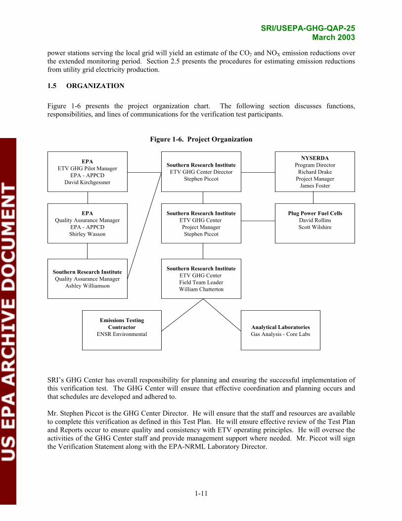
1.5 ORGANIZATION
Figure 1-6 presents the project organization chart. The following section discusses functions, responsibilities, and lines of communications for the verification test participants.
Figure 1-6. Project Organization
EPA ETV GHG Pilot Manager
EPA - APPCD David Kirchgessner
EPA Quality Assurance Manager
EPA - APPCD Shirley Wasson
Southern Research Institute Quality Assurance Manager
Ashley Williamson
Southern Research Institute ETV GHG Center Director
Stephen Piccot
Southern Research Institute ETV GHG Center Project Manager Stephen Piccot
Southern Research Institute ETV GHG Center Field Team Leader William Chatterton
Emissions Testing Contractor
ENSR Environmental Analytical Laboratories Gas Analysis - Core Labs
NYSERDA Program Director
Richard Drake Project Manager
James Foster
Plug Power Fuel Cells David Rollins Scott Wilshire
SRI’s GHG Center has overall responsibility for planning and ensuring the successful implementation of this verification test. The GHG Center will ensure that effective coordination and planning occurs and that schedules are developed and adhered to.
Mr. Stephen Piccot is the GHG Center Director. He will ensure that the staff and resources are available to complete this verification as defined in this Test Plan. He will ensure effective review of the Test Plan and Reports occur to ensure quality and consistency with ETV operating principles. He will oversee the activities of the GHG Center staff and provide management support where needed. Mr. Piccot will sign the Verification Statement along with the EPA-NRML Laboratory Director.
1-11

SRI/USEPA-GHG-QAP-25 March 2003
Mr. Piccot will also have overall responsibility as the Project Manager. He will be responsible for developing the Test Plan and overseeing field data collection activities of the GHG Center’s Field Team Leader, including assessment of the Team Leader’s accomplishment of data quality objectives (DQOs). Mr. Piccot will ensure the procedures outlined in Sections 2.0 and 3.0 are adhered during testing unless modification is required. Such modifications will be explained and justified in the Verification Report. Mr. Piccot will have authority to suspend testing should a situation arise that could affect the health or safety of any personnel. He will also have the authority to suspend testing if quality problems occur or host site or vendor problems arise. Mr. Piccot will be responsible for maintaining effective communications with NYSERDA, Plug Power, EPA-ORD participants, SRI QA team members, and ETV document reviewers.
Mr. William Chatterton will serve as the Field Team Leader. Mr. Chatterton will be responsible for the effective planning, mobilization, and execution of all field-testing activities. He will install and operate measurement instruments, supervise and document activities conducted by the emissions testing contractors, collect gas samples and coordinate sample analysis with the laboratory, and ensure that all QA/QC procedures outlined in Section 2.0 are followed. He will also support Mr. Piccot’s data quality determination and report preparation activities and will submit all results to Mr. Piccot documenting the final reconciliation of DQOs. He will be responsible for ensuring that performance data collected by continuously monitored instruments and manual sampling techniques are based on procedures described in Section 4.0.
SRI’s Quality Assurance Manager, Dr. Ashley Williamson, will review this Test Plan. He will also review the results from the verification test and conduct an Audit of Data Quality (ADQ), described in Section 4.4. Dr. Williamson will prepare a written report of his findings from internal audits and document reviews. These findings will be used to prepare the Verification Report.
Mr. James Foster, Senior Project Manager, will serve as the primary contact person for NYSERDA. Mr. Foster will provide technical assistance and help coordinate this test with the host site and Plug Power as necessary. NYSERDA’s Manager of Power Systems Research, Mr. Richard Drake, will direct Mr. Foster's activities.
Mr. David Rollins of Plug Power will coordinate with SRI throughout this verification and will ensure the SU1 System located at the host site in Lewiston is operating properly and representatively prior to the start of scheduled testing and throughout the entire testing period. He will also provide technical input and guidance on the design and operation of the fuel cell system as needed to effectively plan and complete this verification. Mr. Rollins will coordinate and conduct Plug Power’s review of the Test Plan and the Verification Report, and will provide written comments on both documents to SRI. Mr. Scott Wilshire of Plug Power will oversee the activities of Mr. Rollins.
EPA-ORD will provide oversight and QA support for this verification. The APPCD Project Officer, Dr. David Kirchgessner, is responsible for obtaining final approval of the Test Plan, Verification Report, and Verification Statement. The APPCD QA Manager will ensure review of the Test Plan and Verification Report occurs and that approval is granted once any issues have been satisfactorily resolved.
1.6 SCHEDULE
The tentative schedule of activities for this verification are outlined below.
VERIFICATION TEST PLAN DEVELOPMENT GHG Center internal draft completed December 9, 2002
1-12

NYSERDA and Plug Power review and revision EPA and peer-review and revision
Final Test Plan posted
VERIFICATION TESTING AND ANALYSIS Measurement instrument installation/shakedown Field testing Data validation and analysis
VERIFICATION REPORT DEVELOPMENT GHG Center internal draft development NYSERDA, vendor, and host site review/revision EPA and industry peer-review/revision
Final Report posted
SRI/USEPA-GHG-QAP-25 March 2003
January 13, 2003 March 7, 2003
March 14, 2003
TBD March 28, 2003 TBD April 12, 2003
TBD May 9, 2003
TBD June 13, 2003 TBD July 7, 2003 TBD August 1, 2003
TBD August 29, 2003
1-13

SRI/USEPA-GHG-QAP-25 March 2003
(This page intentionally left blank)
1-14
SRI/USEPA-GHG-QAP-25 March 2003
2.0 VERIFICATION APPROACH
2.1 OVERVIEW
In developing the verification strategy for the SU1 System, the GHG Center has adopted: (1) existing standards for gas-fired turbine and internal combustion (IC) generation equipment; (2) previous peerreviewed DG system evaluations; (3) U.S. EPA methods; (4) professional engineering judgment; and (5) technical input from the verification team. In considering electrical power generation and its quality, the GHG Center acquired some concepts described directly from documents such as:
• The American Society of Mechanical Engineers (ASME) Performance Test Code for Gas Turbines, PTC-22 (2)
• Performance Test Code for Reciprocating Internal Combustion Engines, PTC-17 (3) • Performance Test Code for Fuel Cell Power Systems, PTC-50 (4) • The American National Standards Institute / Institute of Electrical and Electronics
Engineers IEEE Master Test Guide for Electrical Measurements in Power Circuits(1)
• The IEEE Recommended Practices and Requirements for Harmonic Control in Electrical Power Systems (14).
This verification will adopt EPA reference methods described in 40 CFR 60, Appendix A (10) for criteria pollutant and GHG emissions determinations. These generalized methods, however, do not address measurement of the expected low exhaust gas flow rate, low expected NO2 concentrations, high moisture content, and CO2 concentrations in the exhaust streams. The GHG Center will therefore use specialized test methods and modifications to the reference methods as described below.
The GHG Center will conduct short-term emissions and performance testing at three operating loads and extended monitoring at normal site conditions to address the following verification parameters:
Power Production Performance (Section 2.2) • Electrical power output at selected loads, kW • Electrical efficiency at selected loads, % • Total electrical energy generated, kWh
Electrical Power Quality Performance (Section 2.3) • Electrical frequency, Hz • Power factor, % • Voltage THD, % • Current THD, %
Air Pollutant Emission Performance (Section 2.4) • CH4, CO, CO2, NOX, and THC concentrations at selected loads, ppmv, % • CH4, CO, CO2, NOX, and THC emission rates at selected loads, lb/hr, lb/Btu, lb/kWh
Emission Reductions (Section 2.5) • Estimated annual NOX emission reductions, lb NOX/yr • Estimated annual GHG emission reductions, lb CO2/yr
2-1
2.5
SRI/USEPA-GHG-QAP-25 March 2003
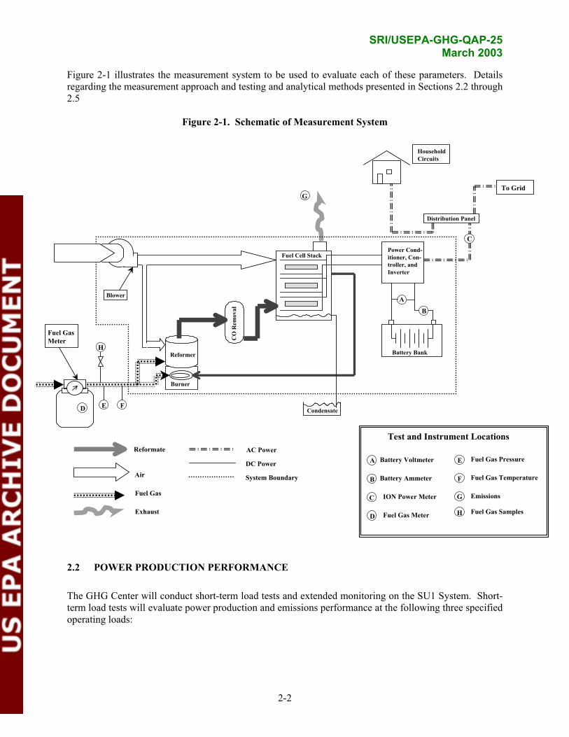
Figure 2-1 illustrates the measurement system to be used to evaluate each of these parameters. Details regarding the measurement approach and testing and analytical methods presented in Sections 2.2 through
Figure 2-1. Schematic of Measurement System
A
E F
G
B
C
D
Fuel Gas
H
Burner
Reformer
CO
Rem
oval
Blower
Fuel Cell Stack
Household Circuits
Distribution Panel
Battery Bank
To Grid
Meter
Power Conditioner, Controller, and Inverter
Condensate
Test and Instrument Locations Reformate AC Power
A Battery Voltmeter E Fuel Gas Pressure DC Power
Air System Boundary B Fuel Gas Temperature Battery Ammeter F
Fuel Gas C Emissions ION Power Meter G
Exhaust D
Fuel Gas Samples Fuel Gas Meter H
2.2 POWER PRODUCTION PERFORMANCE
The GHG Center will conduct short-term load tests and extended monitoring on the SU1 System. Shortterm load tests will evaluate power production and emissions performance at the following three specified operating loads:
2-2

SRI/USEPA-GHG-QAP-25 March 2003
• (1) - 2.5 kW • (2) - 4.0 kW • (3) - 5.0 kW
Each test at each operating load will consist of three individual one-hour runs (load tests) conducted concurrently with the emissions tests described in Section 2.4. Appendix A-1 contains detailed load testing procedures. Appendix A-2 provides a load test log form. After completion of the short-term load tests, extended monitoring of power production performance will commence as described below.
The Field Team Leader will ensure that the SU1 System is operating under steady-state conditions for each load setting during each load test run. For microturbine and engine generator verifications, PTC-22 and PTC-17 (2,3) were followed to set power output, power factor, fuel, and atmospheric operating condition limits that ensure accuracy and repeatability and allow results to be evaluated in common units. The restrictions also minimize electrical efficiency determination uncertainty. ASME has recently published PTC-50 specific to evaluation of fuel cell power systems (4). Based on PTC-50 and review of the SU1 System’s operating data, the GHG Center has developed the permissible variations presented in Table 2-1. Should the values found during a particular test run exceed those in Table 2-1, the Field Team Leader will deem the run invalid and will repeat it.
Note that some permissible variations which the GHG Center will accept for this verification may not be consistent with anticipated PTC-50 values (shown in parentheses in Table 2-1). For example, the 2 percent power output variation expected to be proposed in PTC-50 amounts to only 50 watts when this SU1 System operates at 2.5 kW output. Ongoing monitoring data show that SU1 System power output often varies up to 7 percent from hour to hour. PTC-50’s primary application will be for larger fuel cell systems, and the GHG Center feels that a 5 percent maximum permissible power output variation is a more appropriate compromise for small power generation equipment. An unduly restrictive specification would cause many test runs to be rejected; one that is too loose would yield less meaningful results.
Table 2-1. Permissible Power, Fuel, and Atmospheric Condition Variations
Measured Parameter Maximum Permissible Variation Real power output, kWe ± 5.0 % (± 2.0 %) Total power output, kVA ± 5.0 % (± 2.0 %) Barometric pressure, psia ± 0.5% (± 0.5 %) Inlet air temperature, °F ± 5.0 oF (± 5.0 °F) Gas fuel pressure, psig ± 1.0 % (± 1.0 %) Gas fuel flow, scfm ± 5.0 % (± 2.0 %) Note: Values in parentheses are expected to be consistent with values to be proposed in PTC-50.
2.2.1 Electrical Power Output and Efficiency
At each of the three selected loads, electrical efficiency will be:
HI kW )(14.3412 η = (Eqn. 1)
2-3

SRI/USEPA-GHG-QAP-25 March 2003
Where: η = Efficiency, as proportion, η*100 as percent kW = Average electrical power output, kW, (Eqn. 2) HI = Average heat input using lower heating value, Btu/hr, (Eqn. 3) 3412.14 = Conversion of kW to Btu/hr
Average electrical power output is the mean of the one-minute instantaneous readings gathered over the one-hour sampling period as shown in Equation 2.
n
∑kWi 1kW = (Eqn. 2)
n
Where: KW = Average electrical power output, kW kWi = Instantaneous kW sensor reading during minute i, kW n = Number of 1-minute readings logged by the kW sensor
A field-mounted flow meter system will continuously monitor fuel gas consumption corrected to standard cubic feet per minute (scfm); the GHG Center’s data acquisition system (DAS) will record one-minute averages throughout each test period. These data, combined with laboratory analyses of the fuel lower heating value (LHV), allow determination of the SU1 System’s heat input according to Equation 3.
HI = 60(Vg )LHV (Eqn. 3)
Where: HI = Average heat input using LHV, Btu/hr 60 = Minutes per hour Vg = Fuel flow rate, scfm, (Eqn. 4) LHV = Average fuel gas LHV, Btu/scf
The flow meter system will include a gas meter whose output units are actual cubic feet per minute (acfm). Equation 3 requires corrected flow rate at standard conditions [60 °F, 14.73 pounds per square inch absolute (psia)]. The corrected fuel flow rate is:
Vg =Vm
Pg
7.14
520 Z
std
Z (Eqn. 4)
Tg g
Where: Vg = Fuel flow rate at standard conditions, scfm
Vm = Average volumetric flow rate of fuel gas recorded during the test run, acfm Pg = Fuel gas pressure, psia 14.73 = Gas industry standard pressure, psia 520 = Gas industry standard temperature, oR Tg = Fuel gas absolute temperature, oR
2-4

SRI/USEPA-GHG-QAP-25 March 2003
2-5
Zstd = Compressibility factor at standard pressure and temperature, based on gas analysis performed per ASTM D3588
Zg = Compressibility factor at fuel gas pressure and temperature, based on gas analysis performed per ASTM D3588
The GHG Center will install sensors in the gas pipeline and continuously monitor the fuel gas temperature and pressure during testing. Laboratory analysis of fuel gas samples will supply the required compressibility data. The operator will restore the system to its normal 2.5 kW nominal output at the conclusion of the load test runs. After Plug Power deems that the system is operating normally, the extended monitoring period will commence. The objective of the extended monitoring period is to quantify the SU1 System power quality during internal and external operating cycles and to determine the average power production rate. A one year or longer extended monitoring period would be best for obtaining long-term power production data, but is beyond this verification’s scope. A shorter extended monitoring period which considers the system operating characteristics will provide a reasonable understanding of average power production. Figure 2-2 presents the SU1 System power production data collected by the site operators from May 17 through June 5, 2002. The figure shows typical power output variation and system operating cycles. The GHG Center has not verified the data, but it can be assumed that they represent normal SU1 System operations and can form the basis for a test design.
Figure 2-2. SU1 System Power Output
05/17/02, 17:45 through 06/05/02, 21:45
1.8
2
2.2
2.4
2.6
2.8
3
3.2
3.4
0 50 100 150 200 250 300 350 400 450Operating Hours (Total Hours)
Pow
er O
utpu
t (kW
)
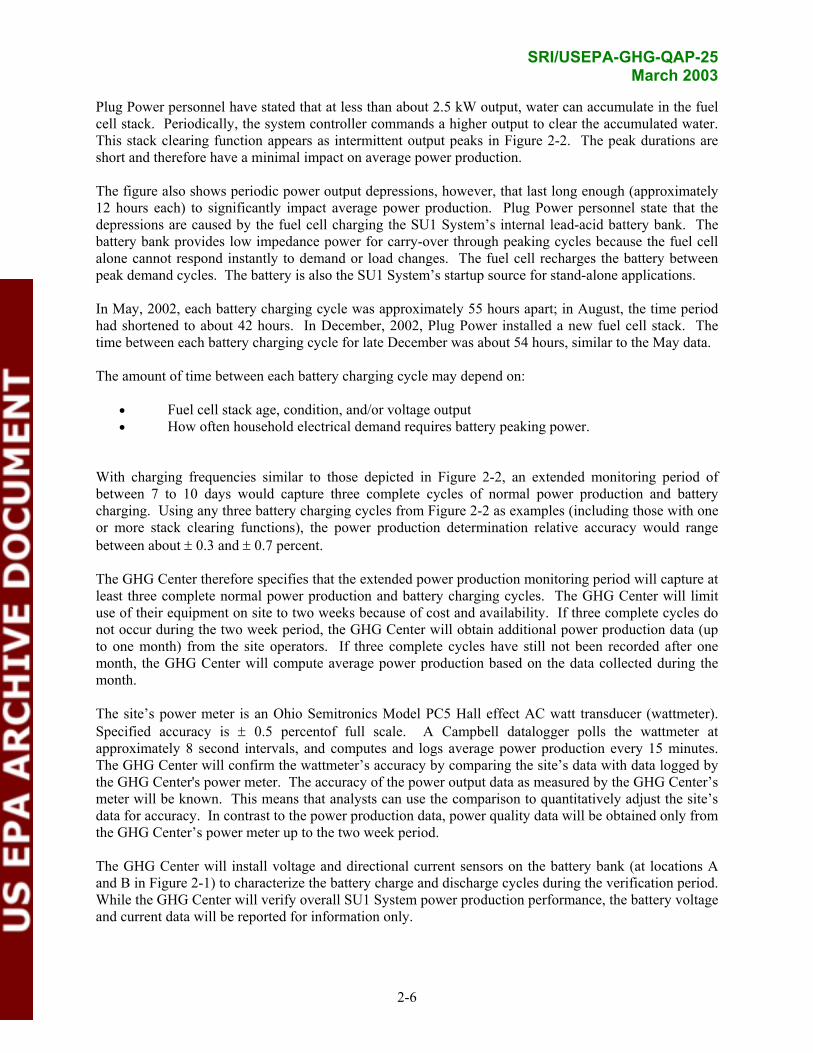
SRI/USEPA-GHG-QAP-25 March 2003
Plug Power personnel have stated that at less than about 2.5 kW output, water can accumulate in the fuel cell stack. Periodically, the system controller commands a higher output to clear the accumulated water. This stack clearing function appears as intermittent output peaks in Figure 2-2. The peak durations are short and therefore have a minimal impact on average power production.
The figure also shows periodic power output depressions, however, that last long enough (approximately 12 hours each) to significantly impact average power production. Plug Power personnel state that the depressions are caused by the fuel cell charging the SU1 System’s internal lead-acid battery bank. The battery bank provides low impedance power for carry-over through peaking cycles because the fuel cell alone cannot respond instantly to demand or load changes. The fuel cell recharges the battery between peak demand cycles. The battery is also the SU1 System’s startup source for stand-alone applications.
In May, 2002, each battery charging cycle was approximately 55 hours apart; in August, the time period had shortened to about 42 hours. In December, 2002, Plug Power installed a new fuel cell stack. The time between each battery charging cycle for late December was about 54 hours, similar to the May data.
The amount of time between each battery charging cycle may depend on:
• Fuel cell stack age, condition, and/or voltage output • How often household electrical demand requires battery peaking power.
With charging frequencies similar to those depicted in Figure 2-2, an extended monitoring period of between 7 to 10 days would capture three complete cycles of normal power production and battery charging. Using any three battery charging cycles from Figure 2-2 as examples (including those with one or more stack clearing functions), the power production determination relative accuracy would range between about ± 0.3 and ± 0.7 percent.
The GHG Center therefore specifies that the extended power production monitoring period will capture at least three complete normal power production and battery charging cycles. The GHG Center will limit use of their equipment on site to two weeks because of cost and availability. If three complete cycles do not occur during the two week period, the GHG Center will obtain additional power production data (up to one month) from the site operators. If three complete cycles have still not been recorded after one month, the GHG Center will compute average power production based on the data collected during the month.
The site’s power meter is an Ohio Semitronics Model PC5 Hall effect AC watt transducer (wattmeter). Specified accuracy is ± 0.5 percentof full scale. A Campbell datalogger polls the wattmeter at approximately 8 second intervals, and computes and logs average power production every 15 minutes. The GHG Center will confirm the wattmeter’s accuracy by comparing the site’s data with data logged by the GHG Center's power meter. The accuracy of the power output data as measured by the GHG Center’s meter will be known. This means that analysts can use the comparison to quantitatively adjust the site’s data for accuracy. In contrast to the power production data, power quality data will be obtained only from the GHG Center’s power meter up to the two week period.
The GHG Center will install voltage and directional current sensors on the battery bank (at locations A and B in Figure 2-1) to characterize the battery charge and discharge cycles during the verification period. While the GHG Center will verify overall SU1 System power production performance, the battery voltage and current data will be reported for information only.
2-6

SRI/USEPA-GHG-QAP-25 March 2003
The following subsections describe the electric power, battery current, battery voltage, fuel flow, fuel temperature, and fuel pressure metering systems. This section concludes with a discussion of the fuel sampling protocol and the laboratory analyses which will provide the heating value and compressibility data required by Equations 3 and 4. Section 3.0 presents the associated data quality objectives, data quality indicators, QA/QC checks, calibrations, and sensor function checks.
2.2.1.1 ION Electrical Power Meter
The GHG Center will measure total electric power output from the SU1 System using a digital power meter, manufactured by Power Measurements Ltd. (Model 7600 ION, 7500 ION, or equivalent). The meter scans all power parameters once per second and sends the data to the DAS. The DAS then computes and records 1-minute averages. Section 4.0 provides further discussion of the DAS. Analysts will enter the 1-minute average power output readings into Equations 1 and 2 to compute electrical efficiency at each load.
Test personnel will install the power meter on the SU1 System’s distribution panel. The installed meter will operate continuously, unattended, and will not require further adjustments. The rated accuracy of the power meter is ± 1.5 percent.
2.2.1.2 Battery Voltage and Current Sensors
The DAS will log battery voltage and current as one-minute averages. When configured to accept a 0 10 volt direct current (VDC) input, each DAS channel’s input impedance is 1.0 x 10⁶ ohms (megohm). The DAS channel is capable of measuring 0 to 60 VDC with a precision 5.0 megohm resistor installed in series with the channel input. This means that for a given 60 VDC input, the voltage drop as measured by the DAS channel will be 10 volts while the voltage drop across the resistor terminals will be 50 volts. With the appropriate engineering scale conversion, the DAS will record the input as 60 volts.
This configuration will allow measurement of the nominal 48 VDC expected at the battery terminals. The channel input accuracy is ± 0.1 percent. Combined with the resistor’s ± 0.01 percent accuracy, overall accuracy for this voltage measurement will be ± 0.1 percent.
The GHG Center will employ a Sypris-W.H. Bell, Model RS-100 bidirectional direct current (DC) transformer-type sensor to measure battery current flow. Similar to the current transformers (CTs) used with the electric power meter, the battery’s primary current conductor passes through the middle of the sensor. When current flows through the primary conductor, the sensor produces a - 4.0 to + 4.0 VDC output, scaled to the conductor’s current direction and magnitude. The RS-100 capacity is 100 amperes ± 1.0 percent.
2.2.1.3 Fuel Gas Meter
The GHG Center will measure actual fuel gas flow with a Rockwell-Invensys Model R-200 diaphragm test meter. An Imac Systems Model 400-10P pulse transmitter, mounted on the meter’s index, combined with an Imac Systems Model R-4 remote totalizer will provide a scaled 4 - 20 mA signal to the DAS. The pulse transmitter system has a resolution of 1 pulse per every 0.01 actual cubic feet. The DAS will record actual gas flow as one-minute averages. Analysts will use computer spreadsheets to calculate corrected standard flow according to Equation 4. The SU1 System’s expected gas consumption at 2.5 and 5.0 kW output will be approximately 0.7 and 1.4 acfm, respectively. The meter capacity is 0 to 3.3 acfm, ± 1.0 percent of reading.
2-7

SRI/USEPA-GHG-QAP-25 March 2003
After correcting each one-minute average actual flow to standard conditions, the GHG Center will compute and report average corrected gas flow by the methodology presented in Equation 2 (substituting Vg,i for kWi).
2.2.1.4 Gas Temperature and Pressure Measurements
Equation 4 requires fuel gas pressure and temperature data to correct the actual gas flow to standard conditions. Center personnel will install a Rosemount Model 3095 mass flow transmitter (3095) and Model 68 resistance temperature detector (RTD) in the gas pipeline adjacent to the fuel gas meter for these measurements. The 3095 incorporates an absolute pressure sensor. It also integrates the pressure sensor and RTD outputs into a common Hart protocol signal. A Rosemount Model 333U Tri-loop interface will convert the Hart signal into separate 4 - 20 mA signals which the DAS will monitor.
The GHG Center expects fuel gas pressure to remain reasonably stable during each test run. The pressure is standard for household applications, or approximately 0.5 psig (about 15.1 psia). The 3095 pressure sensor upper range limit is 800 psia. At a specified span of 20 psia, it is accurate to ± 0.33 percent or ± 0.066 psia. Temperature will vary with the time of year and should range between 45 to 55 oF. The RTD is accurate to ± 0.63 oF at 50 oF. The 3095 process temperature transmitter accuracy is ± 1.0 oF for an overall temperature accuracy of ± 1.63 oF at 50 oF.
2.2.1.5 Gas Composition and Heating Value Analysis
The Field Team Leader will collect fuel gas samples and submit them to a laboratory to obtain the LHV data required by Equation 3 and the compressibility data required by Equation 4. Test personnel will collect at least two samples spaced throughout each short term load testing day. At least two samples spaced throughout each week will be collected during the long term monitoring period.
A tee fitting and ball valve located in the fuel pipeline between the gas metering equipment and the SU1 System will provide access for the 600 milliliter (ml) stainless steel gas sampling canisters. The laboratory evacuates the canisters to prepare them for sampling. Prior to sample collection, test personnel will check the canisters with a vacuum gauge to ensure that they remain under vacuum and are leak free. Canisters that are not fully evacuated will not be used or will be evacuated on site and checked again before use.
Appendices A-8, A-9, and A-10 contain detailed sampling procedures, log, and chain-of-custody forms.
The Field Team Leader will submit the collected samples to Core Laboratories of Houston, Texas for compositional analysis in accordance with American Society for Testing and Materials (ASTM) Specification D1945 (5). This procedure will quantify speciated hydrocarbons including CH4 (C1 through pentane C5), heavier hydrocarbons (grouped as hexanes plus C6+), N2, O2, and CO2. The lab procedure specifies sample gas is injected into a Hewlett-Packard 589011 gas chromatograph equipped with a molecular sieve column and a flame-ionization detector (FID). The column physically separates gas components, the FID detects them, and the instrument plots the chart traces and calculates the resultant areas for each compound. The instrument then compares these areas to the areas of the same compounds contained in a calibration reference standard analyzed under identical conditions. The reference standard areas are used to determine instrument response factors for each compound and these factors are used to calculate the component concentrations in the sample.
2-8

SRI/USEPA-GHG-QAP-25 March 2003
The laboratory calibrates the instruments weekly with the reference standards. During calibrations, the instrument operator generates analytical response factors for each compound. These factors are then programmed into the instrument. Instrument accuracy is ± 0.2 percent full-scale, but allowable method error during calibration is ± 1 percent of the reference value of each gas component. The laboratory recalibrates the instrument whenever its performance is outside the acceptable calibration limit of ± 1 percent for each component. The GHG Center will obtain and review the calibration records.
The laboratory will use the compositional data to calculate the gross (HHV) and net (LHV) heating values (dry, standard conditions), compressibility factor, and the specific gravity of the gas per ASTM Specification D3588 (6). The data quality of the heating value determinations is related to the repeatability of the ASTM D1945 analysis discussed above. Provided the analytical repeatability criteria are met, ASTM D3588 specifies that LHV repeatability is approximately 1.2 Btu/1,000 ft3 or about 0.1 percent. Accuracy is twice this value, or 0.2 percent.
2.2.1.6 Ambient Conditions Measurements
The GHG Center will collect meteorological data to determine if the Table 2-1 maximum permissible limits for electrical efficiency determination are satisfied. The Field Team Leader will install a Vaisala Model HMD60Y integrated temperature/relative humidity sensor and a Setra Model 280e ambient pressure sensor near the SU1 System air inlet plenum for this purpose.
The integrated temperature/humidity unit uses a platinum RTD for temperature measurement. As the temperature changes, the resistance of the RTD changes. This resistance change is detected and converted by associated electronic circuitry that provides a linear (DC 4-20 mA) output signal. The temperature accuracy is ± 1.08 oF. A thin film capacitive sensor measures humidity. The dielectric polymer’s capacitance varies with relative humidity. Internal electronics convert the capacitance change into a linear output signal (DC 4-20 mA). Relative humidity accuracy is ± 2.0 percent, absolute. The barometric pressure sensor (ambient psia) also employs a variable capacitance sensor. As pressure increases, the capacitance decreases; full-scale span is 25.0 psia. Accuracy is ± 1 percent of full scale, or 0.25 psia.
The GHG Center’s DAS will convert the 4-20 mA analog signals to digital format and then store the data as 1-minute averages. After each emission test run, the Field Team Leader will review the data for compliance with the permissible variation limits in Table 2-1.
2.3 POWER QUALITY PERFORMANCE
Electric power users, utilities, and distributors are concerned with a number of power quality issues which power generator operators must address. For example, in grid parallel mode, a generating unit must detect and synchronize with grid voltage and frequency before actual grid connection occurs. The fuel cell must automatically disconnect from the grid under out-of-tolerance operating conditions such as overvoltages, undervoltages, and over/under frequency. The control circuitry also must disconnect and shut the unit down during grid outages to prevent islanding. Also, the system’s delivered power factor should be close to unity (100 percent) to avoid billing surcharges. The unit’s voltage and current harmonic distortion must also be minimized to reduce damage or disruption to electrical equipment (e.g., lights, motors, office equipment).
The generator’s effects on electrical frequency, power factor, and THD cannot be completely isolated from the grid. The quality of power delivered actually represents an aggregate of disturbances already present in the utility grid. For example, locally generated power with low THD will tend to dampen grid
2-9

SRI/USEPA-GHG-QAP-25 March 2003
power with high THD in the test facility’s wiring network. This effect will drop off with distance from the generator. For power factor, the generator’s effects will also change with increasing distance as the aggregate grid power factor begins to predominate.
The GHG Center and its stakeholders developed the following power quality evaluation approach to account for these issues. Two documents form the basis for selecting the power quality parameters of interest and required measurement methods (1, 14). The GHG Center will measure and record the following power quality parameters during the short-term testing and extended monitoring periods:
• Electrical frequency • Voltage • Voltage THD • Current THD • Power factor
The ION power meter (7600 ION or 7500 ION) used for power output determinations will perform these measurements as described in the following subsections.
2.3.1 Electrical Frequency
The ION power meter will continuously measure electrical frequency at the SU1 System’s distribution panel. The DAS will record 1-minute averages throughout all test periods and the GHG Center will report mean frequency as compared to the U.S. standard 60 ± 0.6 Hz (± 1.0 percent). The mean frequency is the average of all the recorded 1-minute data over the test period; sample standard deviation is a measure of dispersion about the mean as follows:
n n
∑ Fi ∑ (F − Fi )2
1 1F = (Eqn. 5) σ F = (Eqn. 6) n n −1
Where: F = Mean frequency for baseline and turbine operating periods, Hz Fi = Average frequency for the ith minute, Hz n = Number of 1-minute readings logged σF = Sample standard deviation in frequency for baseline and turbine operating periods
2.3.2 Generator Line Voltage
The SU1 System generates power at 220 VAC. The electric power industry accepts that voltage output can vary within ± 10 percent of the standard voltage without causing significant disturbances to the operation of most end-use equipment. Deviations from this range are often used to quantify voltage sags and surges.
The ION power meter will continuously measure true root mean square (rms) line-to-line voltage at the SU1 System’s distribution panel. True rms voltage readings provide the most accurate AC voltage representation. The DAS will record 1-minute averages throughout all test periods. The GHG Center will report voltage data for each test period as follows:
2-10

• •
•
SRI/USEPA-GHG-QAP-25 March 2003
Total number of voltage disturbances exceeding ± 10 percent Maximum, minimum, mean, and standard deviation of voltage exceeding ± 10 percent Maximum and minimum duration of incidents exceeding ± 10 percent
Analysts will employ Equations 5 and 6 to compute the mean and standard deviation of the voltage output by substituting the voltage data for the frequency data.
2.3.3 Voltage Total Harmonic Distortion
Harmonic distortion results from the operation of non-linear loads. Harmonic distortion can damage or disrupt many kinds of industrial and commercial equipment. Voltage harmonic distortion is any deviation from the pure AC voltage sine waveform.
The ION power meter applies Fourier analysis algorithms to quantify total harmonic distortion (THD). Fourier showed that one sum of pure sine waves with different frequencies can represent any wave form. He also showed that each contributing sine wave is an integer multiple (or harmonic) of the lowest (or fundamental) frequency. For 60 Hz electrical power in the US, the 2nd harmonic is 120 Hz, the 3rd is 180 Hz, and so on. The types of devices (i.e. capacitors, motor control thyristors, inverters, etc.) connected to the distribution can strongly affect certain harmonics, such as the 5th or 12th.
For each harmonic, the magnitude of the distortion can vary. Typically, each harmonic’s magnitude is represented as a percentage of the rms voltage of the fundamental. The aggregate effect of all harmonics is called THD. THD is the sum of the rms voltage of all harmonics divided by the rms voltage of the fundamental, converted to a percentage. THD gives a useful summary view of the generator’s overall voltage waveform quality.
The ION meter will continuously measure voltage THD up to the 63rd harmonic. The meter’s output value is the result of the following calculation:
63 ∑volti
2THDvolt = 100 * (Eqn. 7)volt1
Where: THDvolt = Voltage THD, % volti = rms voltage reading for the ith harmonic, volts volt1 = rms voltage reading for the fundamental, volts (220, 480, etc.)
The “recommended practices for individual customers” in the IEEE 519 Standard (14) specifies a 5.0 percent maximum voltage THD. The GHG Center will adopt this specification for this verification. The DAS will record 1-minute voltage THD averages throughout all test periods. The GHG Center will report periods for which overall voltage THD exceeded 5.0 percent, mean, and standard deviation per the methods outlined in Equations 5 and 6.
2-11

SRI/USEPA-GHG-QAP-25 March 2003
2.3.4 Current Total Harmonic Distortion
Current THD is any distortion of the pure current AC sine waveform and, similar to voltage THD, can be quantified by Fourier analysis. The current THD limits recommended in the IEEE 519 Standard (14) range from 5.0 percent to 20.0 percent, depending on the size of the generator, the test facility’s demand, and its distribution network design as compared to the capacity of the local utility grid. For example, the standard’s recommendations for a small generating unit connected to a large capacity grid are more forgiving than those for a large generating unit connected to a small capacity grid.
Detailed analysis of the facility’s distribution network and the local grid are beyond the scope of this verification. The GHG Center will, therefore, report current THD data without reference to a particular recommendation. As with voltage THD, the ION power meter will continuously measure current THD. The DAS will record 1-minute current THD averages throughout all test periods. The GHG Center will report mean and standard deviation of current THD per the methods outlined in Equations 5 and 6.
2.3.5 Power Factor
Power factor is the phase relationship of current and voltage in AC electrical distribution systems. Under ideal conditions, current and voltage are in phase, which results in a unity (100 percent) power factor. If reactive loads are present, power factors are less than this optimum value. Although it is desirable to maintain unity power factor, the actual power factor of the electricity supplied by the utility may be much lower because of load demands of different end users. Typical values ranging between 70 and 90 percent are common. Low power factor causes heavier current to flow in power distribution lines for a given number of real kilowatts delivered to an electrical load.
The ION power meter will be used to continuously measure the average power factor for the SU1 System. The DAS will record one-minute averages during all test periods. The GHG Center will report maximum, minimum, mean, and standard deviation per the methods outlined in Equations 5 and 6.
2.3.6 Power Quality Measurement Instruments
The 7600 ION power meter is capable of measuring all power quality parameters. The DAS will record one-minute average measurements. Section 3.0 provides details regarding the instrument, its calibration and additional QA/QC checks (instrument setup, calibration, sensor function checks).
2.4 FUEL CELL EMISSIONS
Field personnel will conduct fuel cell exhaust stack emissions tests for the following air pollutants: NOX (NO and NO2 separately), CO, THCs, and greenhouse gases (CO2 and CH4). The GHG Center has developed a unique approach for evaluating emissions from the Plug Power SU1 System. This approach addresses several sampling complications specific to fuel cell exhaust gas streams that are not typically considered when measuring emissions from combustion sources. Fuel cell exhaust gas characteristics that complicate emissions measurements include the following:
• Extremely low levels of pollutants: NOx and CO concentrations will be in the ppb range. This will require highly sensitive analytical detectors for accurate quantification of these parameters.
2-12

SRI/USEPA-GHG-QAP-25 March 2003
• Low exhaust gas flow rate: Accurate quantification of exhaust gas flow rates will require careful execution of reference method procedures. The accuracy of the subsequent conversion of pollutant emission concentrations (ppm) to mass flow rates (lb/hr) depends on the flow rate accuracy.
• Potential interferences: Relatively high moisture (35 to 40 percent) and CO2 (12 to15 percent) concentrations in the exhaust gas have the potential to interfere withsmall pollutant concentrations.
The GHG Center designed this protocol to address these complications in two ways. First, the sampling system and analytical approach minimizes analytical bias introduced by the three issues outlined above. Second, the protocol specifies well-defined procedures that will allow quantification of sampling system bias and compensation of measured emissions for that bias. The following subsections describe the emissions testing protocol, sampling and analytical procedures, and the rationale for reference method modifications.
To verify SU1 System emissions, the GHG Center will conduct three test runs at each of three power output set points that coincide with the electrical efficiency tests described earlier. During each test run, the System will operate under normal and steady conditions as specified in Table 2-1. The verification report will present individual test run results and the average result of three valid test runs at each load. The report will state average concentrations measured during each test run in units of parts per million volume, dry (ppmvd) or parts per billion volume, dry (ppbvd) where appropriate for NOX, CO, CH4, and THC, and percent for CO2. The report will also present average emission rates for each pollutant in units of pounds per hour (lb/hr).
ENSR International will perform all emissions testing. The testing contractor will provide all equipment, sampling media, and labor needed to complete the testing and will operate under the supervision of GHG Center Field Team Leader following this protocol for quantifying fuel cell emissions. Table 2-2 summarizes the standard U.S. EPA Federal Reference Methods that will be followed. These Reference Methods are well documented in the Code of Federal Regulations (10), and they are used to determine pollutant levels from a wide variety of sources. They include measurement system performance specifications, test procedures, quality control procedures, and emission calculations.
Table 2-2. Summary of Emission Testing Methods
Parameter U.S. EPA Reference Method
Principle of Detection Proposed
Analytical Range Instrument Limit of Detection
O2 3A Electrochemical Cell 0 to 25 % 0.1 % CO2 3A NDIR 0 to 20 % 0.1 %
NO, NO2, NOX 7E Chemiluminescence 0 to 2 ppm 10 ppb
CO 10 NDIR-Gas Filter Correlation 0 to 10 ppm 40 ppb
THC and CH4 18 GC/FID 0 to 20 ppm 50 ppb THC, 20 ppb CH4
Moisture Content 4 Gravimetric Not Specified Not Specified Exhaust gas
volumetric flow rate
2C Differential Pressure 0 to 0.023 “ H2O; ≈ 0 to 10 ft/sec
0.0004 “ H2O; ≈ 1.3 ft/sec
2-13

SRI/USEPA-GHG-QAP-25 March 2003
Each of the instrumental analyzer method includes performance-based specifications for the gas analyzer used. These performance criteria cover span, calibration error, sampling system bias, zero drift, response time, interference response, and calibration drift requirements. The following subsections discuss each test method in more detail. The Reference Methods will not be repeated here, but will be available to site personnel during testing.
2.4.1 Reference Method Modifications
Certain procedural modifications and additions will be made to the Reference Methods listed above to more accurately quantify the low level emissions expected from the SU1 System.
Exhaust Gas Volumetric Flow Rate Exhaust gas velocity will be approximately 8.0 and 4.0 feet per second (ft/sec) at 5.0 kW and 2.5 kW power output, respectively. These low velocities, combined with the small exhaust duct diameter (4 inches), necessitate use of a small-diameter standard pitot (1/8 inch) and an extremely sensitive digital manometer. A digital manometer with a resolution of 0.001 in. H2O will be used (Solomat Zephyr II Model 20, or equivalent). The GHG Center will install a temporary test duct onto the SU1 System’s exhaust fitting to ensure a stable, well-developed, and well-mixed exhaust gas stream.
NOX Emissions
The GHG Center anticipates that SU1 System NOX emissions will be very low which implies that the analyzer span must also be low. Some manufacturer’s data indicate “<0.3 ppmvd” concentrations in the fuel cell stack gas, but these data do not indicate the analyzer’s span nor do they incorporate quantitative information about error. They also may be confounded by method, calibration, CO2/H2O interference, or QA/QC problems.
The presence of CO2 can quench the chemiluminescence effect for certain analyzers, biasing the NOX result low (16). The proportion of NO2 to total NOX can be quite high for low emission sources and the effects of sample train construction materials on that higher proportion of NO2 can be significant (11). Some researchers have found that moisture-removal systems can bias NO2 (and the resulting total NOX) results because NO2 readily dissolves in water (7) while others have not documented such effects (11), possibly because of different residence times in different sample conditioning systems.
In any case, measurement of the expected extremely low NOX emissions will be a challenge, and field verification of the measurements will be essential. The GHG Center proposes inclusion of an additional NO2 to NO converter, on-site generation of low level calibration gases, and certain equipment recommendations. The GHG Center does not endorse the use of any single instrument type, but in certain cases, pre-existing data warrant the use of specific instruments. Additionally, this verification will include a comprehensive sampling system validation test for NOX measurements. This validation procedure is a modification of the Standard Addition technique (18) and will allow the GHG Center to evaluate NOX sampling system bias created by PEM fuel cell exhaust characteristics (low NOX, high moisture, and high CO2) and correct for any bias in the measurements.
Figure 2-3 presents a sampling system schematic. Table 2-3 provides method modification summaries. The following subsections provide details regarding sampling modifications or additions to the standard methods and analytical procedures. Section 3.0 discusses QA/AC checks, analyzer and system calibration procedures, and the NOX Standard Addition validation procedure.
2-14

SRI/USEPA-GHG-QAP-25 March 2003
Figure 2-3. Gas Sampling and Analysis System
Heated Sample Lines
li
GC/
NOx
CO2
CO
O2
Gas
NO2
NO2 to NO
Thermo Electric Moisture Removal System
Condensate
Sample and Calibration Gas Control Manifold
Samp ng Pump
System Exhaust
FID Analyzer
Analyzer
Analyzer
Analyzer
Analyzer
Data Acquisition
System
Unheated Sample Lines
Flow Controller/ Calibration Gas Dilution System
Heated Sampling Probe
System Calibration
Heated 3-way Valve
/ CO Spike Gas
Convertor
Precision Rotameter
Precision Rotameter
Heated teflon lines
Unheated teflon lines
Ascarite Scrubber
NO2 / CO N2 Calibration Gases Spike Gas
2.4.2 Temporary Test Duct, Gaseous Sample Conditioning and Handling
Testers will install a temporary test duct on the SU1 System exhaust outlet which meets EPA Method 1 criteria (no less than 10 duct diameters long). This duct will locate and support the test probes, provide suitable personnel access, and ensure proper exhaust mixing and flow development. Duct material will be new galvanized steel, pre-cleaned with Alcanox (or equivalent) laboratory grade detergent prior to installation.
All gas conditioning and handling system interior surfaces will be made of stainless steel, Teflon or glass to minimize any reactions with the sample gas components. All unheated Teflon tubing will be new or "virgin" Teflon to minimize potential bias introduced by dirty or contaminated sampling system surfaces. Heated Teflon lines indicated in Figure 2-5 will be cleaned immediately prior to the test using Alconox or equivalent laboratory grade cleaner, and then purged with laboratory grade nitrogen. Heated gas transport lines will maintain a gas temperature of no less than 250 oF during all testing.
2-15

SRI/USEPA-GHG-QAP-25 March 2003
Table 2-3. Modifications to Reference Method Specifications
System Component Method Modification or Additional Requirement Reason/Purpose for Modification
Temporary exhaust gas ducta Clean galvanized steel, pre-cleaned with Alcanox (or equivalent) with spike injection, pitot traverse, and sampling ports installed
Spike gas mixing and development of wellbehaved flow for pitot traverses and analyzer sampling probe
Gas Extraction Systema
Heated Teflon sample lines
Precleaned with Alcanox (or equivalent) laboratory grade detergent and purged with nitrogen Minimize bias introduced by contaminated
surfacesUnheated Teflon sample lines New or "virgin" Teflon to be used
NO2 to NO converter
Additional NO2 to NO converter installed near stack
Conversion of NO2 in exhaust gas to NO prior to moisture-removal system
Gas conditioning system
Baldwin Environmental Model M5210 moisture-removal system is specified
Minimize NO2 losses caused by scrubbing during moisture-removal process
Low level pollutant analyzers
NOX and CO analyzers
Ambient level analytical ranges for both analyzers required Lower analytical detection limits
Calibration gas delivery system
Low level calibration gases generated on-site using gas dilution system (EPA Method 205)
Conduct analyzer and sampling system calibrations at ambient levels
Zero gas Analyze and certify zero gas for NOX and CO < 10 ppb
Minimize NOX and CO background effects on analyzer zero calibration
Analytical Validation Systemb Standard Addition Procedure Validate analytical accuracy of system and quantify NO2 losses to scrubbing and/or quenching
a See Section 2.4.2 for details regarding these additional sampling requirements b See Section 3.4.2 for details regarding these additional QA/QC requirements
A vacuum pump on the system’s downstream side will extract exhaust gas from a single point near the center of the 4-inch inside diameter test duct (Figure 2-5). A precision rotameter with a needle valve will control the sampling rate throughout the entire system at approximately 3 standard liters per minute (slm). Limiting the sampling rate to this level provides several benefits. Specifically, this rate optimizes the NO2 to NO conversion efficiency and the low rate minimizes the amount of moisture introduced to the system (exhaust gas moisture content is expected to be around 37 percent). Also, this rate limits the potential bias from NO2 losses within the sampling system because NO2 can adhere to sampling system surfaces. The 3 slm sampling rate will provide sufficient gas for the analyzers.
Extracted gas first passes through a heated 3-way valve where calibration gases are introduced and then through a near-stack NO2 to NO converter (Baldwin development model or equivalent). This converter’s function is to convert the majority of the NO2 fraction of NOX to NO prior to removing moisture from the gas. Because NO is much less soluble in water than NO2, this precaution will help minimize NO2 losses during the moisture-removal process. The converter is constructed of molybdate carbon material, has a rated conversion efficiency of 98 percent, and will be maintained at a temperature of 650 oF during testing.
A heated Teflon sample line conveys the gas stream to a moisture-removal system specifically designed for low-NOX measurement (Baldwin Model M325A/B, or equivalent). The Baldwin system to be used here is a portable unit that incorporates a thermo-electronic chiller that cools gases passing through a glass-coated stainless steel impinger. This instrument is specifically designed for the sampling rates
2-16

SRI/USEPA-GHG-QAP-25 March 2003
desired here (approximately 3 slm), and tests have shown that NO2 losses due to high moisture content in the gas stream are minimal (7).
The clean, dry sample is then transported to a flow distribution manifold where the operator controls sample flow to each analyzer. Calibration gases are routed through this manifold and a Teflon line to the heated 3-way valve near the sample probe. This allows calibration and bias checks to include all components of the sampling system. The distribution manifold also routes calibration gases directly to the analyzers, when linearity checks are made on each.
Testers will use an on-site gas chromatograph and flame ionization detector (GC/FID) to quantify THC and CH4 concentrations. This detector analyzes gases on a wet, unconditioned basis. Therefore, a second, heated sample line will deliver the unconditioned exhaust gases from the stack to the GC/FID.
2.4.3 Gaseous Pollutant Analytical Procedures
A chemilumenescence analyzer (Horiba Model CLA-510SS or equivalent) will continuously determine NOX concentrations. This analyzer catalytically reduces NOX in the sample gas to NO. O3 (normally generated by ultraviolet light) is then used to convert the NO to excited NO2 molecules. The resulting NO2 luminesces in the infrared region. An infrared detector measures the emitted light. The intensity of the emitted energy from the excited NO2 is proportional to the concentration of NO in the sample. An efficiency check of the catalytic converter which changes the various NOX compounds to NO is a part of instrument set up and checkout. Based on preliminary test results from Plug Power, the NOX analyzer will be operated on a range of 0 to 2 ppm. The Field Team Leader will implement analyzer range adjustments in the field to ensure that measured NOX concentrations are within 20 and 100 percent of the analyzer’s full scale.
For CO determinations, a portion of the continuous sample will be passed through a gas filter correlation non-dispersive infrared (NDIR) analyzer (Thermo Environmental Instruments (TEI) Model 48C or equivalent). The analyzer will be equipped with an ASCARITE scrubber to minimize CO2 interference. The NDIR analyzer measures the amount of infrared light that passes through the sample gas versus through the reference cells. Because CO absorbs light in the infrared region, the degree of light attenuation is proportional to the CO concentrations in the sample. Field personnel will set the CO analyzer range at or near 0 to 10 ppm based on Plug Power’s preliminary measurements on the SU1 System. The Field Team Leader will implement modified analyzer ranges during testing if proposed ranges are inadequate.
A second NDIR analyzer (Servomex Model 1415B or equivalent) will measure CO2 concentrations. Similar to the CO analyzer, the NDIR analyzer measures the amount of infrared light that passes through the sample gas versus through the reference cells. Because CO2 absorbs light in the infrared region, the degree of light attenuation is proportional to the CO2 concentrations in the sample. Test personnel will set the CO2 analyzer range at 0 to 20 percent based on Plug Power’s preliminary measurements.
A paramagnetic reaction cell analyzer (Servomex Model 1420B or equivalent) will measure exhaust gas O2. This analyzer’s measuring cell consists of a mass of diamagnetic material which is electronically temperature-controlled to a temperature of 50 oC. The higher the sample O2 concentration, the greater the mass is deflected from its rest position. An optical system connected to an amplifier detects the deflection. A coil of wire surrounds the dumbbell. Current passing through the wire tends to return the dumbbell to its original position. The current applied is linearly proportional to the O2 concentration in the sample. Exhaust gas O2 concentrations are expected to be less than 1 percent, so testers will set the O2 analyzer range at or near 0 to 1 percent.
2-17

SRI/USEPA-GHG-QAP-25 March 2003
Emissions testers will determine CH4 and THC concentrations by Method 18. A continuous stream of exhaust gas will be passed through the an on-site gas chromatograph with flame ionization detector (GC/FID; HP Model 5890 Series II or equivalent). Test operators will analyze no less than three sample injections during each test run at intervals of approximately 20 minutes. Sample injections will be separately analyzed for CH4 and THC. THC concentrations will be quantified and reported as methane. Test operators will perform duplicate analyses on each sample and will calibrate the GC prior to sample analyses with certified CH4 standards.
The Method 18 tests provide concentrations on a wet basis (ppmvw). To convert measured concentrations to a dry basis, stack gas moisture content will be determined in conjunction with each test run using EPA Method 4. Each Method 4 test run will be approximately 60 minutes in duration and will coincide with the emissions test runs.
2.4.4 Determination of Emission Rates
The instrumental testing for CO2, O2, NOX, CO, THC, and CH4 provides exhaust gas concentrations in units of percent for CO2 and O2, ppbvd for NOX and CO, and ppmvd for THC and CH4. Exhaust gas flow rate determinations via Method 2C are required to convert the measured pollutant concentrations to mass emissions in terms of pounds per hour (lb/hr). Test personnel will conduct one stack gas velocity and temperature traverse per emission test run with a calibrated thermocouple, a standard-type pitot tube, and a digital micromanometer. Testers will select the traverse point number and locations in accordance with EPA Method 1A.
Stack gas velocity depends on the average pitot differential pressures, gas molecular weight, temperature, and pressure as follows:
TsV = 49.85 (C p )(Avg[ ∆p ]) (Eqn. 8) s M P s s
Where: Vs = Stack gas velocity, ft/sec Cp = Pitot coefficient, dimensionless ∆p = Average velocity head, inches water Ts = Average stack temperature, oR Ps = Absolute pressure in stack, in. Hg Ms = Molecular weight of stack gas, lb/lb-mole
Volumetric flow rate under standard conditions is:
(Q = 1 A V − Bws ) Ps Tstd 60 (Eqn. 9) std s Pstd Ts
2-18

SRI/USEPA-GHG-QAP-25 March 2003
Where: Qstd = Volumetric flow rate, dscf/min Vs = Stack gas velocity, ft/sec A = Stack cross sectional area, ft2
Bws = Stack gas moisture content, % Ps = Absolute pressure in stack, in. Hg Pstd = Standard pressure, 29.92 in. Hg Ts = Average stack absolute temperature, oR Tstd = Standard temperature, 532 oR 60 = Seconds per minute
EPA Method 4 test runs conducted in conjunction with each emission test will supply stack gas moisture content (Bws). These data, combined with the direct CO2 and O2 determinations (Method 3A), and the assumption that the balance of the stack gas is N2, allow calculation of the stack gas molecular weight (Ms) required in Equation 8.
Analysts will convert measured pollutant concentrations as ppmvd (or ppbvd) to pounds per dry standard cubic foot (lb/dscf) using the following unit conversion factors:
CH4: 1 ppmvd = 4.150E-08 lb/dscf CO: 1 ppmvd = 7.263E-08 lb/dscf
CO2: 1 ppmvd = 1.141E-07 lb/dscf NOX: 1 ppmvd = 1.194E-07 lb/dscf NOX (emissions are quantified as NO2)
THC: 1 ppmvd = 4.150E-08 lb/dscf THC (emissions are quantified as CH4)
After conversion of measured pollutant concentrations to mass units (lb/dscf), emission rate values are:
E poll = C poll K pollQstd 60 (Eqn. 10)
Where: Epoll = Pollutant emission rate, lb/hr Cpoll = Average pollutant concentration during the test run, ppmv Kpoll = Pollutant ppmvd to lb/dscf (conversion factor, see above) Qstd = Standard dry volumetric flow rate, dscf/min (Eqn. 9) 60 = Minutes per hour
The verification report will present the mean of the three test results at each load factor as the average emission rate for that load factor. The GHG Center will then normalize emission rates for each pollutant to system power output in terms of lb/kWh as follows:
Enorm =E j (Eqn. 11)
kWh j
Where: Enorm = Normalized emission rate, lb/kWh Ej = Mean emission rate at load condition j, lb/hr kWhj = Mean power production rate at load condition j
2-19

SRI/USEPA-GHG-QAP-25 March 2003
The mean of the three normalized emission rates will be reported as the average emission rate in lb/kWh.
All of the sampling and analytical procedures and reference methods cited here contain QA/QC procedures that will be followed to evaluate data quality. Section 3.0 contains the procedures and associated data quality objectives.
2.5 ELECTRICITY OFFSETS AND ESTIMATION OF EMISSION REDUCTIONS
2.5.1 Estimated Annual Emission Reductions for the Lewiston Residence
Without on-site generation of electricity with the SU1 System, all of the electrical power demand at the residence is met by the local utility (Niagara Mohawk (NiMo)). Electricity generation from central power stations defines the baseline power scenario for this facility, and emissions of NOX and CO2 generated by these stations represent the baseline emissions in the absence of the SU1 System. With the SU1 System operating, some of the power demand of the residence is met through on-site generation. Under this scenario, less power is purchased from the utility grid. If emissions of CO2 and NOX with the SU1 System scenario are lower than the emissions associated with the baseline scenario, then a reduction in emissions would be realized under the SU1 System scenario.
For this verification, emissions from the SU1 System will be compared with the baseline scenario to estimate annual NOX and CO2 emission levels and reductions (lb/yr). These pollutants were considered because CO2 is the primary greenhouse gas emitted from combustion processes and NOX is a primary pollutant of regulatory interest. Reliable emission factors for electric utility grid and boilers are available for both gases. Emission reductions are computed as follows:
Annual Emission Reductions (lb/yr) = [Baseline Scenario Emissions] – [SU1 System Scenario Emissions]
Annual Emission Reductions (%) = Annual Emission Reductions (lb/yr) / [Baseline Scenario Emissions]* 100
The following 3 steps describe the methodology used.
Step 1 - Determination of the Annual Electrical Energy Profile of the Lewiston Residence
The first step in estimating emission reductions is to determine the annual electrical energy demand of the residence on a monthly basis. The NYSERDA partnership conducting the long-term demonstration at this residence closely monitors the home's demand. These data will be compiled for the calendar year 2002 as shown in Table 2-4. The monthly residence demand values will represent the baseline scenario (all demand is met using power purchased from the grid).
After verification testing, Table 2-4 will be completed to estimate the distribution of energy demand as supplied by the systems in the baseline and SU1 System scenarios. The power values reported for the SU1 System will be determined based on the average power output measured during full load tests and the number of operating days in each month. Also, the power generated by the SU1 System will be derated using average monthly air temperatures for the site. This is accomplished by using the trends observed during the verification test. Using this verification data, an electrical energy efficiency curve is developed as a function of ambient temperatures and the efficiency levels at the average monthly temperatures
2-20

SRI/USEPA-GHG-QAP-25 March 2003
Table 2-4 Electrical Demand of the Lewiston Residence
Monthly Residence Electrical Demand
kWh
Baseline Scenario SU1 System Scenario
Power Supplied By Utility Grid
kWh,Grid
Power Supplied by SU1 System
kWh,SU1
Power Supplied by Grid kWh,Grid
Jan Feb Mar Apr May June July Aug Sept Oct Nov Dec
Annual Total
2,899 2,376 2,106 1,955 1,934 1,805 1,923 1,829 1,803 2,767 2,295 2,347
26,039
2,899 2,376 2,106 1,955 1,934 1,805 1,923 1,829 1,803 2,767 2,295 2,347
26,039 Est
imat
ed fo
r eac
h m
onth
usi
ng p
ower
outp
ut v
erifi
ed d
urin
g te
stin
g
Cal
cula
ted
as m
onth
ly d
eman
d m
inus
pow
er su
pplie
d by
SU
1 Sy
stem
Step 2 – Emissions Estimate For the SU1 System
Using the energy production data for the SU1 System, emissions associated with this system were estimated as follows:
1 SU 1 SU 1 SU ER * kWhE = (Eqn. 12) where:
ESU1 = SU1 System emissions, lb/yr kWh,SU1 = Electrical energy generated by SU1 System, Table 2-4, kWh,SU1 ERSU1 = SU1 System emission rate, lb/kWh
The CO2 and NOX emission rates defined above are equivalent to the average full load emission rate determined during the verification test.
Step 3 - Emissions Estimate For the Utility Grid
Emissions associated with electricity generation at central power stations is defined by the following equation:
EGrid = kWhGrid, ER * 078 .1 * Grid (Eqn. 13)
2-21

SRI/USEPA-GHG-QAP-25 March 2003
where:
EGrid = grid emissions (lb/yr) kWh,Grid = electricity supplied by the grid, Table 1-4 (kWh) 1.078 = transmission and distribution system line losses ERGrid = NY ISO displaced emission rate (lb/kWh)
The kWh,Grid variable shown above represents the estimated electricity supplied by the utility grid under the baseline scenario and the SU1 System scenario (Table 2-4). These values are increased by a factor of 1.078 to account for line losses between central power stations and the end user.
Defining the grid emission rate (ERGrid) is complex, and the methodology for estimating this parameter is continuously evolving. The following discussion provides a brief background on the concept of displaced emissions, and presents the strategy employed by the GHG Center to assign ERGrid for this verification.
EPA has long recognized that clean energy technologies have the potential for significant emission reductions through displaced generation. However, a robust and analytically sound method to quantify the potential of displaced emissions has yet to be developed. Displaced generation is defined as the total electrical output (measured in kWh) from conventional electricity sources that is either displaced by or avoided through the implementation of energy efficient measures. Displaced emissions is defined as the change in emissions (measured in lb) that results when conventional electrical generation is displaced by energy efficient measures. On-site heat and power generation with a distributed energy technology (e.g., SU1 System) is an example of a clean energy source, provided its emissions are less than conventional sources. DG systems can result in displaced generation, and ultimately displace emissions.
Several different methodologies have been developed and employed by various organizations to estimate emissions displaced by on-site electricity generation. Although there are many variations of such methodologies, they are all derived from the average emission rate method, the marginal unit method, or historical emissions/generation data.
• The average emission rate method uses the average emission rate of electricity generating units in a particular region or nationally. It is usually based on the average emission characteristics of all electricity generating units or fossil-fired units only, and is often derived from historic generation and emissions data or projections of future generation and fuel use patterns. This approach is most widely used due to its simplicity and wide availability of average rates for many U.S. regions. Unfortunately, there is little or no correlation between the average emission rate and the emission rate at which the emissions are displaced by energy efficient measures. As a result, estimates of emissions impacts can be inaccurate and may not adequately reflect the realities of power markets.
• The marginal unit method is an attempt to improve on the average emission rate approach by identifying a particular unit or type of unit that may be displaced. Similar to the average emission rate method, the average emission characteristics of the displaced units are applied to total electricity saved to estimate displaced emissions. The marginal unit method assumes that at any point in time, the marginal unit, by virtue of being the most expensive generating unit to operate, will be the unit that is displaced. Although this approach conceptually appears to be more reasonable than simply using an average emission rate, identifying the marginal unit is difficult, particularly in regions with large and frequent variations in hourly electricity demand.
2-22

SRI/USEPA-GHG-QAP-25 March 2003
• Displaced emissions are also estimated using statistical techniques based on historical data. This approach seeks to forecast how displaced emissions arise from observed changes in electricity demand/supply, instead of identifying the average or marginal emission rate of particular units. This approach requires statistical modeling, and data such as regional generation, emissions, and electricity demand. Its primary limitation is that actual site-specific and electricity control area specific data must be available.
EPA has been developing a newer approach that utilizes region/time specific parameters to represent average displaced emission rate (ADER). The ADER methodology accounts for the complexities of electricity markets in assessing how displaced emissions result from changes in electric demand or supply, and produces regional, national, short-term, and long-term estimates of displaced emissions of CO2, NOX, SO2, and Hg from electric generation. The results of the ADER analysis are not currently available; as such, the GHG Center is unable to apply this methodology for this verification. However, at the suggestion of the EPA project officer leading this effort, a similar approach, developed by the Ozone Transport Commission (OTC) has been adopted for this verification to estimate displaced emissions, and is described below.
OTC is a multi-state organization focused on developing regional solutions to the ground-level ozone problem in the Northeast and Mid-Atlantic region of the U.S., with special emphasis on the regional transport of ground-level ozone and other related pollutants. It was created by Congress in 1990, and consists of the jurisdictions within Connecticut, Delaware, D.C., Maine, Maryland, Massachusetts, New Hampshire, New Jersey, New York, Pennsylvania, Rhode Island, Vermont, and Virginia. OTC has recently developed an Emission Reduction Workbook (Workbook) to provide a method of assessing the emissions impacts of a range of energy policies affecting the electric industry (19). The geographic focus of the Workbook is the three northeastern electricity control areas: Pennsylvania/New Jersey/Maryland (PJM), the New York ISO (NY ISO), and ISO New England.
The three energy programs evaluated by the Workbook are: (1) programs that displace generation (e.g., DG or DG-CHP systems), (2) programs that alter the average emission rate of the electricity used in a state or region (e.g., emissions performance standard), and (3) programs that reduce emission rates of specific generating units (e.g., multi-pollutant regulations applied to existing generating units). To evaluate these programs, the Workbook contains default displaced emission rates for the three northeastern control areas. The default displaced emission rates are divided into three time periods: near term (2002-2005), medium term (2006-2010), and long term (2011-2020). For this verification, the shortterm default emission rates for the NY ISO control area will be used to represent the ERGrid variable shown in Equation 13.
The near-term rates for the NY ISO are summarized in Table 2-5. These rates were compiled using the PROSYM electricity dispatch model, and are reported to be representative of actual operations because the identity of generating units that constitute each regional power system are known with a relatively high level of certainty.
2-23

SRI/USEPA-GHG-QAP-25 March 2003
Table 2-5. Displaced Emission Rates For the NY ISO (2002)
NOx (lb/kWhe) CO2 (lb/kWhe) Ozone season weekday a 0.0021 1.37 Ozone season night/weekend b 0.0028 1.67 Non-ozone season weekday c 0.0021 1.46 Non-ozone season night/weekend d 0.0028 1.61 a Average of all hourly marginal emission rates during weekdays, May through September, 7:00 am through 10:59 pm b Average of all hourly marginal emission rates during all nights, May through September, 11:00 pm through 6:59 am, and all weekend days during this period c Average of all hourly marginal emission rates during weekdays, October through April, 7:00 am through 10:59 pm d Average of all hourly marginal emission rates during all nights, October through April, 11:00 pm through 6:59 am, and all weekend days during this period
PROSYM is a chronological, multi-area electricity market simulation model that is often used to forecast electricity market prices, analyze market power, quantify production cost and fuel requirements, and estimate air emissions. It simulates system operation on an hourly basis by dispatching generating units each hour to meet load. The simulation is based on unit-specific information on the generating units in multiple interconnection areas (unit type and size, fuel type, heat rate curve, emission and outage rates, and operating limitations), and detailed data on power flows and transmission constraints within and between ISOs. Because the simulation is done in chronological order, actual constraints on system operation (such as unit ramp times and minimum up and down times) are taken into account. The resulting emission rates in one control region take into account emission changes in neighboring regions. PROSYM has been used by many organizations, including the EPA and Department of Justice to pursue New Source Review violations, DOE, numerous utility companies, Federal Energy Regulatory Commission (FERC), and Powering the South organization to simulate electric power system in the Southern U.S.
OTC generated the displaced emission rates for the Northeast control areas by first performing a “base case” model run, simulating plant dispatch across all three control areas for the year. OTC then performed three “decrement” model runs. In one decrement run, all hourly loads in PJM were reduced by 1 percent; loads in ISO NE, and NY ISO were not reduced. In another decrement run, loads in ISO NE were reduced by 1 percent, and in the third, NY ISO loads were reduced. To calculate marginal emission rates for different periods, OTC calculated the total difference in kWhs generated between the base case and decrement case and the total difference in emissions, and then divided the emissions by kWhs to derive the marginal emission rate for the time period. It should be noted that marginal rates shown in Table 2-5 takes into account changes in generation in all areas resulting from the load reductions in the target DG use area. This includes analysis of emissions changes across six interconnected control areas: PJM, NY ISO, ISO NE, Maritimes, Ontario, and Quebec.
2-24
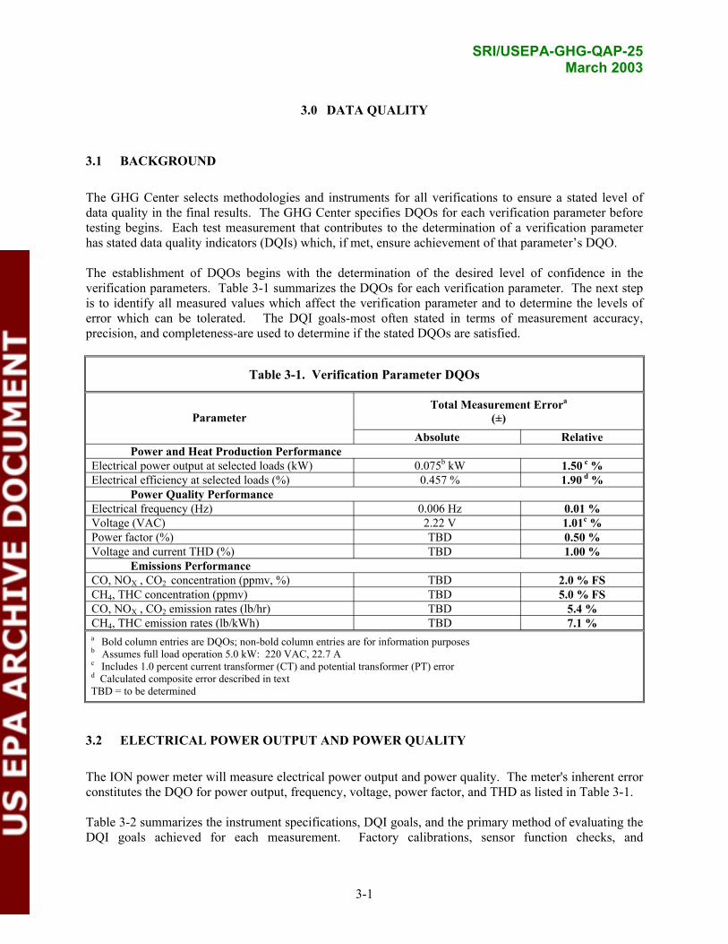
SRI/USEPA-GHG-QAP-25 March 2003
3.0 DATA QUALITY
3.1 BACKGROUND
The GHG Center selects methodologies and instruments for all verifications to ensure a stated level of data quality in the final results. The GHG Center specifies DQOs for each verification parameter before testing begins. Each test measurement that contributes to the determination of a verification parameter has stated data quality indicators (DQIs) which, if met, ensure achievement of that parameter’s DQO.
The establishment of DQOs begins with the determination of the desired level of confidence in the verification parameters. Table 3-1 summarizes the DQOs for each verification parameter. The next step is to identify all measured values which affect the verification parameter and to determine the levels of error which can be tolerated. The DQI goals-most often stated in terms of measurement accuracy, precision, and completeness-are used to determine if the stated DQOs are satisfied.
Table 3-1. Verification Parameter DQOs
Parameter Total Measurement Errora
(±) Absolute Relative
Power and Heat Production Performance Electrical power output at selected loads (kW) 0.075b kW 1.50 c % Electrical efficiency at selected loads (%) 0.457 % 1.90 d %
Power Quality Performance Electrical frequency (Hz) 0.006 Hz 0.01 % Voltage (VAC) 2.22 V 1.01c % Power factor (%) TBD 0.50 % Voltage and current THD (%) TBD 1.00 %
Emissions Performance CO, NOX , CO2 concentration (ppmv, %) TBD 2.0 % FS CH4, THC concentration (ppmv) TBD 5.0 % FS CO, NOX , CO2 emission rates (lb/hr) TBD 5.4 % CH4, THC emission rates (lb/kWh) TBD 7.1 % a Bold column entries are DQOs; non-bold column entries are for information purposes b Assumes full load operation 5.0 kW: 220 VAC, 22.7 A c Includes 1.0 percent current transformer (CT) and potential transformer (PT) error d Calculated composite error described in text TBD = to be determined
3.2 ELECTRICAL POWER OUTPUT AND POWER QUALITY
The ION power meter will measure electrical power output and power quality. The meter's inherent error constitutes the DQO for power output, frequency, voltage, power factor, and THD as listed in Table 3-1.
Table 3-2 summarizes the instrument specifications, DQI goals, and the primary method of evaluating the DQI goals achieved for each measurement. Factory calibrations, sensor function checks, and
3-1

SRI/USEPA-GHG-QAP-25 March 2003
reasonableness checks in the field (listed in Tables 3-2 and 3-3) will document achievement of the DQI goals. The QA/QC procedures identified in Tables 3-2 and 3-3 are described in the following sections.
The power meter manufacturer will issue a calibration certificate which shows compliance to IEC 687 S0.2 and ANSI C12.20 CA0.2. Consistent with ISO 9002-1994 requirements, the manufacturer will supply calibration documents that certify National Institute of Standards and Technology (NIST) traceability. The GHG Center will review the certificate and traceability records to ensure that the instrument meets or exceeds the accuracy specifications listed in Table 3-2. Note that the accuracy standard for kW, compounded with the ± 1.0 percent accuracy specification for the current and potential transformers, yields the ± 1.5 percent DQO specified in Table 3-1.
The power meter is designed and marketed for electric utility custody transfer applications. Its calibration records are reported to be valid for a minimum of one year of use, provided the manufacturer-specified installation and setup procedures are followed. GHG Center personnel will follow installation, setup, and QC procedures detailed in Appendices A-3 and A-4.
GHG Center personnel will perform checks in the field for two key measurements-voltage and current output-which are directly related to the power output measurement. The Field Team Leader will measure distribution panel voltage and current at the beginning of the verification period. He will use a digital multimeter (DMM) and compare voltage and current readings to the power meter readings as recorded by the DAS. The Field Team Leader will obtain a minimum of five individual voltage and current readings for the given load. The power meter voltage and current accuracies are ± 1.01 percent while the DMM is ± 1.0 percent. The percent difference between the DMM reading and the power meter reading must be within ± 2.01 percent for voltage and current. In these cases, the power meter will be deemed to be functioning properly.
Comparisons of the power meter readings as recorded by the GHG Center’s DAS with the power output recorded by the fuel cell control panel will constitute the reasonableness check. The power meter and control panel readout should range from 4.5 to 5.0 kW at full load.
3.3 EFFICIENCY
Electrical efficiency requires determination of electrical power output and fuel heat input. Fuel heat input requires determination of standard flow rate and fuel LHV. Standard flow rate requires determination of actual flow rate, fuel gas pressure, temperature, and compressibility ratios. Determination of total measurement error requires propagation of the individual contributing measurement errors, each with their own characteristic absolute and relative errors. Appendix A-15 presents the error propagation methods to be used in this verification.
Table 3-4 applies the concepts to estimate the electrical efficiency compounded errors. The table includes the referenced equations, contributing measurements, expected measured values, and instrument or compounded errors.
3-2

SRI/USEPA-GHG-QAP-25 March 2003
Table 3-2. Measurement Instrument Specifications and DQI Goals
Data Quality Indicator Goals
Measurement Variable Operating Range Expected in Field
Instrument Type /
Manufacturer
Instrument Range
Instrument Rated Accuracy
Frequency of Measurements Accuracya Completeness
How Verified / Determined
(see Table 3-3)
Electrical Power Output and Quality
Power 0 to 5 kW
Electric Meter/ Power Measurements 7600 ION, 7500 ION, or equivalent
0 to 260 kW ± 1.50c % reading
DAS records 1-min averages
± 1.50 % readingc
95 % valid 1-min averages for short-term tests; 80 % valid 1-min. averages for extended monitoring period
Review manufacturer calibration certificates; perform sensor function checks in field; conduct reasonableness checks for voltage, current, and DAS
Voltage 120 V, single phase 0 to 600 V ± 1.01 % reading ± 1.01 %
reading
Frequency 60 Hz 57 to 63 Hz ± 0.01 % reading ± 0.01 % reading
Current 0 to 22.7 amps 0 to 250 amps ± 1.01 % reading ± 1.01 % reading
Voltage THD 0 to 100 % 0 to 100 % ± 1 % FS ± 1 % FS
Current THD 0 to 100 % 0 to 100 % ± 1 % FS ± 1 % FS
Power Factor 0 to 1.0 (100 %) 0 to 1.0 (100 %) ± 0.5 % reading ± 0.5 % reading
Ambient Meteorological Conditions
Ambient Temperatureb 20 to 80 oF
Vaisala HMD 60Y0
-40 to 140 oF ± 1.08 oF ± 1.08 o F Review manufacturer calibration certificates; perform independent check of temperature and pressure sensors
Relative Humidityb 0 to 100 % 0 to 100 %
± 2 % 0 to 90 % (RH), ± 3 % 90 to 100 % (RH)
± 3 %
Ambient Pressure 14.0 to 14.7 psia SETRA Model
280E or equiv. 0 to 25 psia ± 1.0 % FS ± 1.0 % FS
(continued)
3-3

SRI/USEPA-GHG-QAP-25 March 2003
Table 3-2. Measurement Instrument Specifications and DQI Goals (continued)
Data Quality Indicator Goals
Measurement Variable
Operating Range Expected in Field
Instrument Type / Manufacturer
Instrument Range
Instrument Rated
Accuracy
Frequency of Measurements Accuracya Completeness
How Verified / Determined
(see Table 3-3)
Fuel Input
Volumetric Flow Rate
0.7 to 1.4 acfm; 0.6 to 1.3 scfm
Diaphragm Test Meter / Rockwell-Invensys R-200
0 to 3.3 acfm; 0 to 3.1 scfm ± 1.0 % reading
DAS records 1-min averages
± 1.0 % reading
95 % valid 1-min averages for short-term tests; 80 % valid 1-min. averages for extended monitoring period
Review manufacturer’s NIST traceable calibration records; perform reasonableness checks
Gas Pressure 14.5 to 15 psia Pressure Transmitter / Rosemount 3095 0 to 20 psia ± 0.33 % at 20
psia ± 0.33 % FS
Gas Temperature 45 to 60 oF RTD / Rosemount 68
and 3095 transmitter 40 to 60 oF ± 1.63 oF at 50 oF
± 1.63 oF at 50 oF
Fuel Gas LHV
94 to 98 % CH4 (900 to 1005 Btu/scf)
Gas Chromatograph / HP 589011 0 to 100 % CH4
± 3.0 % accuracy and ± 0.2 % repeatability for CH4; ± 0.1 % repeatability for LHV
Min. 2 samples per day during short-term test periods
± 0.2 % for LHV
100 % for short-term load tests
Repeatability check: Duplicate analyses on the same sample
FS: full-scale a Accuracy goal represents the maximum error expected at the operating range. It is defined as the sum of instrument and sampling errors. b These variables are not directly used to assess DQOs, but are used to determine if DQIs for key measurements are met. They are also used to form conclusions about the system performance. c Includes instrument error, 1.0 percent current transformer (CT) error, and 1.0 percent potential transformer (PT) error.
3-4

SRI/USEPA-GHG-QAP-25 March 2003
Table 3-3. Summary of QA/QC Checks
Measurement Variable QA/QC Check When
Performed/Frequency Expected or Allowable
Result
Response to Check Failure or Out of
Control Condition
Power Output
Instrument calibration by manufacturera Beginning and end of test ± 0.35 % reading
Identify cause of any problem and correct or replace meter
Sensor diagnostics in field Beginning and end of test Voltage within ± 2.01, current
within ± 3.01 % of reading
Identify cause of any problem and correct or replace meter Identify cause of any
Reasonableness checks Throughout test 4.5 to 5.0 kW at full load problem and correct or replace meter
Fuel Flow Rate
Instrument calibration by manufacturera Beginning and end of test ± 1.0 % reading
Identify cause of any problem and correct or replace meter
Reasonableness checks Twice during each day of short-term testing
Manual gas reading standard flow within 7.34 % of DAS standard flow
Identify cause of any problem and correct or replace meter
Duplicate analyses At least once for each performed by load test and on one Refer to Table 3-5 and 3-6 Repeat analysis
Fuel Gas Composition and Heating Value
laboratorya blind audit sample Confirm canister is fully evacuated
Before collection of each sample
Canister pressure < 6.0 psia (17.7 “Hg vacuum) Reject canister
Calibration with gas standards by laboratory
Prior to analysis of each lot of samples submitted ± 1.0 % for CH4 Repeat analysis
Independent performance check with blind audit samplea
Two times during test period
± 3.0 % for each gas constituent Recalibrate instrument
Reasonableness check Identify cause of any with ambient pressure Prior to testing ± 0.32 psia problem and correct, or
Fuel Gas Pressure sensor replace meter
Instrument calibration by manufacturera Prior to testing ± 0.07 psia at 20 psia (0.33 %
relative error)
Identify cause of any problem and correct, or replace meter
Fuel Gas Temperature
Instrument calibration by manufacturera Prior to testing ± 1.63 oF at 50 oF (0.31 %
relative error)
Identify cause of any problem and correct, or replace meter
Reasonableness check with ambient temperature sensor
At least once during testing ± 4 °F
Identify cause of any problem and correct, or replace meter
Ambient Meteorological Conditions
Instrument calibration by manufacturer or certified laboratory
Beginning and end of test Temp: ± 1.08 oF Pressure: ± 1.0 % FS RH: ± 3 %
Identify cause of any problem and correct, or replace meter
Reasonableness checks Once per day during load tests
Recording should be comparable with handheld digital temp/RH meter
Identify cause of any problem and correct, or replace meter
a Results of these QA checks will be used to reconcile DQIs
3-5

SRI/USEPA-GHG-QAP-25 March 2003
Table 3-4.
Value (%) g
g
g
std
g
1.199 acfm 15.0 psia 510 oR 0.9980
0.9979
0.012acfm 0.05 psia 1.63 oR 0.00200
0.00200
1.00 0.33 0.31 0.20
0.20
1.245 scfm 0.014 scfma
(1.245*0.0114) 1.14a
950 Btu/scf 1.9 Btu/scf 0.20
70,965 Btu/hr 823.2 Btu/hra
(70,965*0.0116) 1.16a
Power Output, kW 5.0 kW 0.75 kW 1.50ηe,
24.04 % 0.457 %a
(24.04*0.0190) a,b
a
bDQO for electrical efficiency
Electrical Efficiency Error Propagation and DQO
Contributing Measurements Expected Absolute Error Relative Error
Actual fuel flow rate, VFuel gas pressure, PFuel gas temperature, TFuel gas compressibility factor @ standard conditions, ZFuel gas compressibility factor @ actual conditions, Z
Fuel flow rate at standard conditions, V, requires Equation 4 and these measurements
Eqn. 4 result:
LHV, Btu/scf Heat input, HI, requires Equation 3, this measurement, and the Equation 4 result Eqn. 3 result: Electrical Efficiency, requires Equation 1, this measurement, and the Equation 3 result Eqn. 1 result:
1.90
Errors compound per Appendix A-15
The electrical efficiency DQO will be 1.90 percent, as shown above and in Table 3-1. The DQI goals listed in Table 3-2 are directly linked to the DQO achievement because if DQIs are met, the instruments and measurements will achieve the listed accuracies. If the test campaign achieves each of the listed accuracies, analysts can reasonably conclude that the DQO is achieved in turn.
For the power meter, Section 3.2 discussed the QA/QC procedures to be performed to assess achievement of DQI goals. The following subsections describe the QA/QC procedures for the remaining measurements.
3.3.1 Natural Gas and Fuel Flow Rate Quality Assurance
A service contractor will calibrate the diaphragm-type fuel gas meter with NIST-traceable volume provers at a minimum of 4 points within the specified meter range. This will include full flow, minimum flow, and two intermediate flows. The resulting calibration certificate will indicate measured readings, reference readings, and the percent difference between the diaphragm gas meter and the reference meter. The average percent difference will represent the overall accuracy of the meter. GHG Center personnel will review the calibration to ensure satisfaction of ± 1.0 percent accuracy specification.
The Field Team Leader will perform at least two gas meter reasonableness checks per test day during the short-term test periods. He will measure the time required for the meter to register 1.0 acf (10 meter index revolutions) of gas flow during an emissions test run by observing the meter’s index. He will then convert that flow to standard conditions based on the gas temperature and pressure recorded by the DAS. The resulting manually obtained corrected flow should agree with that recorded by the DAS within 7.34 percent (two times the rated accuracy of the meter). Appendix A-5 contains a detailed procedure and log form.
3-6

SRI/USEPA-GHG-QAP-25 March 2003
3.3.2 Gas Pressure and Barometric Pressure Quality Assurance
The manufacturers will calibrate the Setra ambient pressure and Rosemount 3095 fuel gas pressure transducers prior to testing. The resulting calibration certificates will be NIST-traceable; GHG Center personnel will review the calibration to ensure satisfaction of the accuracy specifications for each unit. The Field Team Leader will perform reasonableness checks by first checking the Setra pressure sensor against atmospheric pressure reported by the local airport (corrected for site elevation). He will then compare the Setra and Rosemount readings while both are subject to atmospheric pressure. Agreement of the two units within 0.32 psia will show that the pressure sensors are operating properly. Appendix A-7 contains the procedure and log form.
3.3.3 Gas Temperature and Ambient Temperature Quality Assurance
The manufacturers will calibrate the Rosemount 3095 transmitter/ Model 68 RTD, and the Vaisala ambient temperature/RH sensor prior to testing. The resulting calibration certificates will be NISTtraceable. GHG Center personnel will review the calibration to ensure satisfaction of the ± 1.63 °F at 50 oF specification for the gas temperature sensor, and the ± 1.08 oF specification for ambient temperature.
As a reasonableness check prior to testing, the GHG Center will compare the gas and ambient temperature sensors' DAS readings with a hand-held digital thermometer while all three sensors are exposed to ambient air. Agreement within ± 4 °F will show that the sensors are operating properly. Appendix A-7 contains the procedure and log form.
3.3.4 Fuel Gas Analyses Quality Assurance
QA/QC procedures for assessing gas composition data quality include duplicate analyses on at least one sample collected during each load condition (designated by the Field Team Leader), review of laboratory instrument calibrations, analysis of a blind audit gas sample, and confirmation of canister pressure prior to sampling. The primary method of reconciling the accuracy goal consists of comparing the laboratory reported values with the audit gas reference values. The method of reconciling the precision goal will be based on duplicate analysis results.
During field testing, the GHG Center will supply one blind/audit gas sample to the laboratory for analysis. The audit gas will be an independent Natural Gas Processors Association (GPA) Reference Standard manufactured by Scott Specialty Gases with a certified analytical accuracy of ± 2 percent. The audit gas will be shipped to the test location and the Field Team Leader will collect a canister sample of it immediately after one of the fuel gas samples is collected. The audit sample will be shipped to the laboratory with the other fuel samples. The laboratory will analyze the audit sample in duplicate. The GHG Center will compute the average result from the two analyses and will compare the results to the certified concentration of each constituent. Allowable error, which is the sum of the instrument calibration criteria and the analytical accuracy of the audit gas, must be less than ± 3.0 percent for each gas constituent.
Duplicate analyses must conform to ASTM Specification D1945 repeatability guidelines. These guidelines vary according to the component’s concentration in fuel gas as illustrated in Table 3-5. Repeatability is the difference between two successive results obtained by the same operator with the same apparatus under same operating conditions. According to the method, repeatability or the absolute difference (Abs. Diff.) between results for the same sample, must not exceed the values shown in Table 35. These specifications are selected as the precision goal for the verification test samples. The average
3-7
SRI/USEPA-GHG-QAP-25 March 2003
difference of all fuel gas samples for which duplicate analysis is performed will represent the actual precision achieved.
Table 3-5. ASTM D1945 Repeatability Specifications
Component Concentration (mol %)
Repeatability / DQI goal (Absolute difference between 2 results)
0 to 0.1 ± 0.01 0.1 to 1.0 ± 0.04 1.0 to 5.0 ± 0.07 5.0 to 10 ± 0.08 over 10 ± 0.1
Using these guidelines and the anticipated ranges of gas component concentrations, Table 3-6 summarizes the target repeatability goals for primary gas components (components with greater than 1.0 percent concentrations) for the duplicate analyses. The GHG Center will report the average differences between all duplicate results as the achieved precision.
Table 3-6. DQIs for Anticipated Component Concentrations
Gas Component Expected
Concentration Range (mol %)
DQI Repeatability Goal (absolute difference of 2
results) Butane 0.1 - 0.5 n/a Ethane 3.0 - 5.0 0.08
Heptane < 0.1 n/a Hexane < 0.1 n/a Methane 90 - 98 0.20 Pentane < 0.1 n/a Propane 1.0 - 3.0 0.07
Additional QA/QC checks include instrument calibrations and confirmation of canister pressures prior to sampling. The analytical laboratory conducts the calibrations on a weekly basis or whenever equipment changes are made on the instrument with a Natural Gas GPA Reference Standard. ASTM Specification D1945 criteria for calibration states that consecutive analytical runs on the gas standard must be accurate to within ± 1 percent of the certified concentration of each component. The GHG Center will require the laboratory to submit calibration results for each day samples are analyzed.
The Field Team Leader will confirm proper sample canister evacuation with a vacuum gauge prior to fuel gas sample collection. Any canisters with absolute pressures greater than 6.0 psia (17.7 in. Hg vacuum) will not be used for sampling or will be re-evacuated and rechecked.
ASTM Specification D3588 (6) provides for calculating gas LHV and compressibility factor based on the gas compositional analyses. The GHG Center will therefore evaluate the data quality of these parameters based on compositional analyses errors discussed above. ASTM D 3588 specifies calculation procedures for gas analysis repeatability. ASTM states that the LHV difference between initial and duplicate analyses performed by the same operator on the same gas sample should exceed two times the repeatability in only 5 percent of all trials. For this verification, two times the repeatability will represent the measurement uncertainty. If repeated analyses achieve the Table 3-5 criteria, natural gas LHV repeatability should be approximately 1.2 Btu/mcf, or about 0.1 percent. This measurement’s uncertainty goal (or DQI) will therefore be 0.2 percent.
3-8

SRI/USEPA-GHG-QAP-25 March 2003
The GHG Center will use Equations 14 and 15, as derived from ASTM D 3588, to evaluate the achieved measurement uncertainty. If it is less than 0.2 percent, the DQI will be achieved.
ninitδLHV = ∑[(LHV − LHV j
dup )δx dup ]2
(Eqn. 14)jj =1
δLHV 2 * %err = 100 (Eqn. 15)LHV init
Where: δLHV = LHV repeatability LHVinit = Total LHV result for the initial analysis, Btu/scf LHVj
dup = LHV for component j from the duplicate analysis, Btu/scf δxj
dup = Molecular fraction difference for component j between initial and duplicate analyses n = Number of components analyzed %err = Measurement uncertainty, percent
Additional QA/QC checks include instrument calibrations and confirmation of canister pressures prior to sampling. The analytical laboratory conducts the calibrations on a weekly basis or after significant instrument changes with a Natural Gas GPA Reference Standard. ASTM Specification D1945 states that consecutive gas standard analytical runs must be accurate to within ± 1 percent of the certified concentration of each component. The GHG Center will require the laboratory to submit calibration results for each day samples are analyzed.
The Field Team Leader will confirm proper sample canister evacuation with a vacuum gauge prior to fuel gas sample collection. Any canisters with absolute pressures greater than 6.0 psia (17.7 in. Hg vacuum) will not be used for sampling or will be re-evacuated and rechecked.
3.4 EMISSIONS TESTING QA/QC PROCEDURES
This verification will use the EPA reference methods listed Table 2-2 to quantify criteria pollutant and GHG emission rates. The reference methods specify sampling methods, calibration methods, and data quality checks which assure that the acquired data meets required quality goals. These methods ensure that run-specific quantification of instrument and sampling system drift and accuracy occurs, and that testers repeat runs if specific performance goals are not met. Based on reference method requirements, the DQOs for concentration measurements are ± 2 percent for NOX, CO, and CO2, and ± 5 percent for THC and CH4. The data quality indicator goals required to meet these DQOs will consist of assessing the sampling system accuracy and drift as outlined in Table 3-7.
3-9

SRI/USEPA-GHG-QAP-25 March 2003
Table 3-7. Instrument Specifications and DQI Goals for Stack Emissions Testing
Instrument Specifications Data Quality Indicators
Measurement Variable Instrument Type or Method
Instrument Accuracya
Frequency of Measurements
Overall Sampling System Accuracy Completeness How Verified /
Determinedb
Microturbine and Engine CHP Emissions
NOX Concentrations
Chemilumenescense analyzer ± 1 % FS
1-minute averages (DAS polls analyzer outputs at 5second intervals)
± 2 % FS includes sampling system bias corrections)
100 % is 3 valid runs at each specified load)
Follow EPA Method calibration and system performance check criteria
CO Concentrations NDIR analyzer ± 1 % FS
± 2 % FS (includes sampling system bias corrections)
CO2 / O2 Levels; Stack Gas Molecular Weight
NDIR (CO2) / paramagnetic or equivalent (O2)
± 1 % FS ± 2 % FS (includes sampling system bias corrections)
CH4, THC Concentrations GC / FID ± 0.1 % FS Once per test run ± 5 % FS
Water Content Gravimetric ± 0.2 % FS (FS = 100%)
Once per load condition ± 5 % FS
Stack Gas Flow Rate
Pitot and Thermocouple
Pitot ∆p: ± 1.0 % Thermocouple: ± 1.5 % of average stack temperature
Once per test run ± 5 % FS NIST-traceable calibrations
a Instrument accuracy is a function of the selected range or full-scale (FS). See Table 2-2 for a complete list of anticipated instrument ranges. b For a full description, see Table 3-8.
3-10

SRI/USEPA-GHG-QAP-25 March 2003
The GHG Center will assess emissions data quality, integrity, and accuracy with a series of measurement system calibrations and quality control checks. The reference method QC checks vary between methods and are pollutant-specific. Table 3-8 lists the QC checks required for each parameter, how often testers will perform them, the maximum allowable result, and the corrective measures for failed checks. Similar to the electric power performance parameters, the DQI goals and QC checks listed in Tables 3-7 and 3-8 are directly linked to the achievement of the emission testing DQOs listed in Table 3-1 because, if they are met, the instruments and measurements will achieve the listed accuracies. The DQOs will be achieved if each of the listed accuracies are achieved.
Table 3-8. Summary of Emissions Testing QC Checks
Measurement Variable Calibration/QC Check When Performed/
Frequency Expected or Allowable
Result Response to Check Failure or Out
of Control Condition
NOX
NO2 to NO converter efficiency test Once before testing Efficiency > 90 %
required Repair or replace analyzer
NOX bias test (Standard Addition Procedure) *
Once before and once following testing
System bias (NO2 loss) in the range of 1 to 15 % Apply system bias correction
NOX, CO, CO2, O2
Analyzer calibration error test Daily before testing ± 2 % of analyzer span Repair or replace analyzer
System bias checks* Before each test run ± 5 % of analyzer span Correct or repair sampling system
Calibration drift test After each test run ± 3 % of analyzer span Repeat test
CH4 and THC
Duplicate analysis* Each sample ± 5 % difference Repeat analysis of same sample
Calibration of GC/FID with gas standards
Prior to analysis of the three samples submitted for this test
± 5 % for each compound Repeat calibration
Sample Gas Transfer Lines
Material and condition inspection Immediately prior to testing
Unheated lines are virgin Teflon; heated lines have been cleaned
Clean and/or replace tubing as needed
Zero Gas Inspect calibration certificate Immediately prior to testing
Certification specifically states total NOX < 10.0 ppb
Obtain proper zero gas
Test Duct Inspect Immediately prior to testing At least 12 diameters long; cleaned prior to testing
Replace and/or clean as needed
Stack Gas Flow
Standard Addition Procedure* Once during testing ± 10 % difference Correct or repair sampling system
Pitot tube inspection and leak check
Once before and once after testing See 40CFR60 Method 2c Select different pitot tube
Micromanometer calibration
Once before and once after testing ± 1.0 % of reading Repair or replace instrument
Thermocouple Calibration Once after testing
± 1.5 % at average stack temperature recorded during final test run
Adjust average stack temperatures for all test runs; recalculate stack flow rates
* Results of these checks will be used to reconcile data quality indicators
3.4.1 Analyzer and Sampling System QA/QC Procedures
The reference methods used here (listed in Table 2-2) detail the standard procedures listed in Table 3-8; they will not be repeated here in their entirety. The following paragraphs provide specific procedure descriptions where needed to highlight those applicable to this verification.
3-11

SRI/USEPA-GHG-QAP-25 March 2003
NO2 Sampling System and Zero Gas
GHG Center personnel will verify that the sampling system umbilicals, tubing, and manifolds have been cleaned or are constructed of virgin Teflon. The calibration gas manifold and/or regulators must incorporate check valves to prevent atmospheric O2 from contaminating the NO2 calibration gas. Testers must also follow proper calibration gas line and pigtail purging procedures to prevent crosscontamination. The zero gas for the NOX sampling system must be analyzed and certified to contain less than 10 ppbv NOX or CO. The Field Team Leader will inspect the zero gas calibration certificate prior to testing.
NO2 Converter Efficiency Test
The NOX analyzer converts any NO2 present in the gas stream to NO prior to gas analysis. For this verification, testers will install an additional converter near the stack which will convert most NO2 to NO prior to gas conditioning. This is important during low NOX measurements to minimize NO2 loss in the sampling system umbilical and moisture-removal system. Testers will conduct a converter efficiency test prior to testing. They will determine converter efficiency for the overall sampling system according to the EPA approved alternative procedure (9). The converters will not be evaluated separately. The procedure specifies introduction of an appropriate EPA Protocol 1 NO2 calibration gas to the system (approximately 1 to 2 ppm NO2 in N2 for this test series). Testers will record analyzer response every minute until the response stabilizes. The converters will be accepted if the recorded response is within 90 percent of the certified gas value. Testers will repair or replace one or both of the converters prior to testing if the NOX measurement system fails the efficiency test.
Calibration Error, System Bias, and Calibration Drift Tests
Calibration error, drift, and system bias tests verify CO, CO2, NOX, and O2 measurement accuracy and will occur at the beginning of each day of testing. All calibration gas mixtures will conform to EPA Protocol 1. Testers introduce a suite of calibration gases directly to each analyzer and record the analyzer responses. Gas concentrations for CO2, NOX, and O2 include zero, 40 to 60 percent of span, and 80 to 100 percent of span. CO concentrations include zero and approximately 30, 60, and 90 percent of span. Analyzer response to any calibration gas must be within ± 2 percent of span.
Before and after each test, testers will introduce zero- and mid-level calibration gases to the sampling system at the probe and record the response. System bias is the comparison between these responses and the calibration error responses recorded earlier. The sampling system is acceptable if system bias is less than ± 5 percent of span for each parameter. Comparison of the pre- and post-test system bias calibrations quantifies each analyzer’s drift. Drifts in excess of ± 3 percent are unacceptable and the test run will be repeated.
The low expected levels and analyzer spans for CO, NOX, and O2 require low calibration gas concentrations. Very low concentrations of NO2 in N2 are especially unstable. Because of this, testers will employ a dynamic gas dilution system to generate specific calibration gas concentrations on site. They will follow EPA Method 205 procedures which specify that gas concentrations must be within ± 2.0 percent of the predicted value after dilution. The Method 205 procedure is not repeated here, but test personnel will perform all of the required QA/QC checks (including field evaluation of the dilution system). Method 205 specifies certified Protocol 1 calibration gases (one for each parameter), pure N2, and a mass flow controller for accurate gas dilution (Environics Series 6100 computerized multi-gas calibration system, or equivalent) to generate the low-level calibration gases.
3-12

SRI/USEPA-GHG-QAP-25 March 2003
After all of the continuous analyzer calibrations are completed and prior to verification test runs, testers will perform a modified NOX sampling system bias check in the form of the Standard Addition Procedure. This will evaluate total system NOX measurement, including the exhaust gas stream and sampling conditioning effects, as introduced in Section 2.4.1. See Section 3.4.2 below for a detailed discussion.
GC/FID Calibration
GC/FID procedures performed according to EPA Method 18 will determine concentrations of CH4 and THC. Test personnel will calibrate the GC/FID prior to sample analysis with certified CH4 standards. Analyses results must be within ± 5 percent. Each analysis includes the following quality assurance procedures outlined in Section 40 CFR, Part 60, Appendix A, Method 18, Section 7.4.4 - Quality Assurance:
• Duplicate injection of each sample aliquot with agreement of all injections to ± 5 percent of the mean;
• Three point calibration curves based on least-squares regression analysis; • Calibration curves developed prior to analysis; and • Agreement of all calibration points with the theoretical value to ± 5 percent.
Testers will perform a triplicate mid-point calibration after all samples have been analyzed. If the asanalyzed value for any compound detected in the test program does not agree within ± 5 percent of its pretest value, testers will generate a full post-test calibration curve. Analysts will then base all reported concentrations on the average of the pre- and post-test calibration points.
Instrumental Analyzer Data Completeness and Reasonableness Checks
The GHG Field Team Leader will review the chart traces (or a line chart representation of the digital DAS file) for each instrumental analyzer at the completion of each test run. The data must be reasonable and complete for each analyzer. Some criteria are:
• The trace must fall entirely within the boundaries of the instrument span; there are noflattened peaks at high concentrations.
• The trace must move smoothly and continuously from concentration to concentration; there are no abrupt steps or extended flat lines.
• The data must be 100-percent complete, defined as no gaps in the chart trace for eachanalyte.
The GHG Field Team Leader will initial each day’s chart. For digital DAS, he will obtain a disk copy of the data file and make the appropriate entry in the test log book.
Exhaust Gas Flow Rate
Exhaust gas flow rate determination includes exhaust CO2, H2O, and O2 concentrations, velocity (differential pressure across a pitot tube); and gas temperature measurements. The GHG Field Team Leader will review O2 and CO2 instrumental analyzer data and calibrations at the end of each test day. Review criteria will be as described previously for the instrumental analyzers. He will also review exhaust gas moisture field data for conformance with EPA Method 4 practices.
Emissions test operators will certify that the pitot tubes meet applicable requirements for dimensional accuracy using the design criteria detailed in Method 2C. Also, in accordance with Method 2C calibration criteria, they will perform pre- and post-test thermocouple calibrations by subjecting the
3-13

SRI/USEPA-GHG-QAP-25 March 2003
thermocouples used during testing to the average temperature found during testing and comparing the readings to a NIST-traceable reference thermometer. For acceptable results, the thermocouple reading must be within 1.5 percent of the reference thermometer. 40 CFR Part 60, Appendix A, Method 2, Section 10.3.1 presents specific thermocouple calibration details.
Prior to and following testing, a calibration laboratory will subject the digital micromanometer to a series of pressures traceable to NIST. The lowest pressure available is approximately 0.001 psig, or 0.028 in. H2O (6.89 Pa). This differential pressure across a pitot is equivalent to approximately 10.8 ft/sec at exhaust gas conditions, which is higher than that expected during the test campaign. To address this issue and to check linearity at lesser pressures, GHG Center personnel will subject the micromanometer to a series of pressures between 0 and 0.028 in. H2O as measured by a “Hook Gage” with 0.001 in. H2O accuracy. This procedure will generate a calibration curve. Digital micromanometers are sometimes subject to zero drift caused by changes in ambient temperature. During testing, the micromanometer will be manually zeroed by operators prior to each pitot traverse.
3.4.2 NOX Sampling System Bias Test and Exhaust Flow Rate Verification (Standard Addition Procedure)
3.4.2.1 NOX Sampling System Bias Test
The sampling system bias test conducted during normal Reference Method calibrations verifies the entire system's response to known calibration standards. The procedure assesses sampling system integrity and analyzer accuracies, but it does not evaluate the affects that moisture and CO2 may have on overall system bias for low NOX measurement. To evaluate NOX sampling system bias, test operators will inject a calibration gas spike with known CO and NO2 concentrations into the exhaust duct as shown in Figure 31. The known concentration of CO in the spike gas will serve as a control agent because the emissions measurement industry widely accepts that high moisture and CO2 concentrations do not bias CO measurements (provided the CO analyzer is a gas filter correlation NDIR instrument).
Figure 3-1. Exhaust Gas Spiking Technique
rotameter
NO2 spike gas A
Precision
or mass flow controller
/ CO
8 Exhaust duct diameters
Exhaust flow
Sample line to analyzers Exhaust duct
3-14

SRI/USEPA-GHG-QAP-25 March 2003
During constant (steady-state) power production, the fuel cell’s exhaust gas flow rate, composition, and pollutant concentrations will be reasonably constant because the reaction kinetics within the fuel cell stack must be constant. Under stable operations, instrumental analyzers at location A in figure 3-1 will report steady concentrations of the various pollutants. A spike gas mixed into the exhaust gas flow will produce an upscale incremental change (delta) at an analyzer if it contains a higher pollutant concentration than that already existing in the exhaust gas. The spike gas flow required to produce a given CO delta depends on the stack gas flow and spike gas CO concentration as follows:
∆
spike
m c
m ∆
− =
1
1
2 (Eqn. 16)
spikec
Where: m2 = Spike flow rate, acfm m1 = Exhaust gas flow rate, acfm ∆ = Upscale concentration change (delta), ppm cspike = Spike gas concentration, ppm
Assuming the manufacturer’s estimated exhaust gas flow at 5 kW power production and a given CO concentration in the spike gas, the following table shows the spike gas flow required to produce the given delta at the CO analyzer.
Table 3-9. Spike Gas Flow Rates for a Given Incremental Changea
CO Delta, ppm Spike Flow, slm 0.75 2.506
2 6.711 4 13.514 6 20.408
10 34.483 a Assumes 1,000 standard liter per minute (slm) exhaust gas flow, 300 ppm CO in the spike gas
If the test operator adjusts the rotameter such that the analyzer records a 0.75 ppm CO delta, the spike gas will be flowing at exactly 2.506 slm. In effect, the exhaust gas stream quantitatively dilutes the spike gas to a level which the operator can control by adjusting the controller flow rate. The exhaust gas will dilute any other gases present in the spike gas stream in exactly the same ratio.
If, in addition to the CO, the spike gas contains a known concentration of NO2, the delta expected at the NOX analyzer will also be directly dependent on its concentration, the exhaust gas flow, and the spike gas flow as follows:
c= ∆ spikem2 (Eqn. 17)
+ m2m1
3-15

SRI/USEPA-GHG-QAP-25 March 2003
Table 3-10 illustrates this by showing the change in NO2 concentration expected at the analyzer for the spike gas flow rates presented in Table 3-9.
Table 3-10. NO2 Delta for Given Spike Gas Flow Ratesa
Spike Flow, slm NO2 Delta, ppm 2.506 0.125 6.711 0.333 13.514 0.667 20.408 1.000 34.483 1.667
a Assumes 1000 standard liter per minute (slm) exhaust gas flow, 50 ppm NO2 in the spike gas
The operator can adjust the rotameter to produce a 0.75 ppm delta at the CO analyzer and the spike gas will be flowing at 2.506 slm. Given a 50 ppm NO2 concentration in the spike gas, the NOX analyzer should record a delta of 0.125 ppm.
Immediately prior to and following the short-term emissions and power production verification tests, GHG Center personnel will introduce a suitable two-component (CO and NOX) calibration gas into the temporary exhaust duct through a probe. The probe’s location will be at least 8 diameters from the sampling probe to ensure good gas mixing. Test personnel will follow the reference method procedures to ensure that no stratification exists at the sampling location.
At a NOX analyzer span of 2.0 ppm, the spike gas concentrations and flow values discussed here will provide sufficient data to develop a five-point calibration curve for the NOX analyzer which includes the “< 0.3 ppm concentrations” expected by the manufacturer. This procedure will represent the NOX sampling system bias check, and the calibration curve will allow the GHG Center to correct results for the measured bias, if any, caused by exhaust gas characteristics. The log form is presented in Appendix A11.
3.4.2.2 Exhaust Gas Flow Rate Verification
The standard addition procedure described above will also allow exhaust gas flow rate verification. With a known spike gas flow rate, the exhaust gas flow rate is related to the spike and exhaust gas CO upscale concentration change as follows:
m1 = m2 (cspike ∆ − )
(Eqn. 18)∆
Where: m1 = Exhaust gas flow rate, acfm
m2 = Spike flow rate, acfm ∆ = Upscale concentration change (delta), ppm cspike = Spike gas concentration, ppm
3-16

SRI/USEPA-GHG-QAP-25 March 2003
Test operators will employ a mass flow controller with ± 1.0 percent accuracy. This uncertainty, compounded by subraction, division, and multiplication with the ± 1.0 percent spike gas calibration certification and ± 2.0 percent analyzer accuracy will yield ± 5.01 percent accuracy for this flow determination method.
At least once during the test campaign, the Field Team Leader will compare the exhaust gas flow rate determined from the standard addition method with that obtained by the pitot traverse. Agreement within ± 10.01 percent will imply that the pitot traverse flow measurements are acceptable. Appendix A-6 contains the log form.
3.5 INSTRUMENT TESTING, INSPECTION, AND MAINTENANCE
GHG Center personnel, the Field Team Leader, laboratories, and/or contracted test organizations will subject all test equipment to the pre- and post-test QC checks discussed earlier. Before the equipment leaves the GHG Center or analytical laboratories, operators will assemble and test it as anticipated to be used in the field. They will operate and calibrate all controllers, flow meters, computers, instruments, and other sub-components of the measurements system as required by the manufacturer and/or this Test Plan. Any faulty sub-components will be repaired or replaced before being transported to the test site. Test personnel will maintain a small amount of consumables and frequently needed spare parts will be maintained at the test site. The Field Team Leader and Project Manager will handle major subcomponent failures on a case-by-case basis.
3.6 INSPECTION/ACCEPTANCE OF SUPPLIES AND CONSUMABLES
Field personnel will use Natural Gas Reference Standard gases to calibrate the GC used for fuel analyses and for submittal of a blind audit sample. The suppliers certify audit gas concentrations to within ± 2 percent of the tag value. Copies of the audit gas certifications will be available on-site during testing and archived at the GHG Center.
Calibrations will employ EPA Protocol 1 gases supplied either by the dilution system described above or directly from cylinders. EPA Protocol gas specifications require the actual concentration to be within ± 2 percent of the certified tag value. Copies of the EPA Protocol gas certifications will be available on-site.
3-17

SRI/USEPA-GHG-QAP-25 March 2003
(this page intentionally left blank)
3-18

SRI/USEPA-GHG-QAP-25 March 2003
4.0 DATA ACQUISITION, VALIDATION, AND REPORTING
4.1 DATA ACQUISITION AND STORAGE
Test personnel will acquire the following types of data during the verification:
• Continuous measurements i.e., gas pressure, gas temperature, power output and quality, and ambient conditions, to be collected by the GHG Center’s DAS
• Fuel gas composition, heating value, compressibility factor, and moisture content from canister samples collected by the Field Team Leader and submitted to laboratory for analysis
• Volumetric gas flow measurements collected by the Field Team Leader • Emission measurements data collected by contractor and supervised by the Field
Team Leader.
The Field Team Leader will also take site photographs and maintain a daily test log which includes the dates and times of setup, testing, teardown, and other activities.
The Field Team Leader will submit digital data files, gas analyses, chain-of-custody forms, and the daily test log to the Project Manager. The Project Manager will initiate the data review, validation, and calculation process. These submittals form the basis of the Verification Report presenting data analyses and results in table, chart, or text format as suited to the data type. The Verification Report’s conclusions will be based on the data and the resulting calculations. The GHG Center will archive and store all data in accordance with the GHG Center QMP.
4.1.1 Continuous Measurements Data Acquisition
An electronic DAS will collect and store continuous process and ambient meteorological data. Core components of the DAS are an Allen-Bradley (AB) Model SLC 5/05 programmable logic controller (PLC) and a Gladiator Unix-based data acquisition computer data server. Figure 4-1 is a schematic of the DAS.
The PLC brings all analog and digital signals from the measurement sensors together into a single realtime data source. The DAS can accommodate any combination of up to 16 analog signal channels with 4 to 20 mA current or ± 10 VDC voltage inputs. Sensors can also provide digital signals via the ModBus network to the DF1 interface unit. This converts the ModBus data to the AB “DF1” protocol which is compatible with the PLC. The PLC nominally polls each sensor once per second and converts the signals to engineering units. It then computes 1-minute averages for export to the TOGA and applies a common time stamp to facilitate data synchronization of all measurements.
4-1

SRI/USEPA-GHG-QAP-25 March 2003
Figure 4-1. DAS Schematic
(s)
Remote or Local Connection Through Ethernet or Modem
4 - 20 MA current loops to analog output sensors
Modbus Sensors
Remote or Local Computer
Data Acquisition System
The data server records information from the PLC and contains the software for programming the PLC (i.e., data sampling rates, engineering unit conversions, calibration constants). Its UNIX operating system writes all PLC data to a My-SQL relational database for export to spreadsheet, graphics, and other programs. This database is ODBC-compliant, which means that almost any MS Windows program can use the data. The data server includes an external modem and Ethernet card for remote and local communications. The user accesses the data server during normal operations with a portable laptop or remote computer via its communications port, Ethernet link, or telephone connection. Spreadsheets allow the user to download the entire database or only that portion which has been added since the last download. The user then conducts data queries (i.e., for certain times, dates, and selected data columns) on the downloaded data as needed.
During the verification testing, GHG Center personnel will configure the DAS to acquire the process variables listed in Table 4-1. Note that the Field Team Leader will acquire the fuel cell power command and date/time data manually at the start of each test run.
4-2

SRI/USEPA-GHG-QAP-25 March 2003
Table 4-1. Continuous Data to be Collected for Fuel Cell Evaluation
Sensor / Source Measurement Parameter Purposea Significance Rosemount pressure sensor and transducer Fuel gas pressure, psia P System performance parameter
Rosemount temperature sensor and transducer Fuel gas temperature, °F P System performance parameter
Vaisala Model HMP60YO Ambient temperature, oF P System performance parameter Ambient relative humidity, % RH P System performance parameter
Setra Model 280E Ambient pressure, psia P System performance parameter
Electric Meter 7600 ION and 7500 ION
Voltage output, volts P System performance parameter Current, amps P System performance parameter Power factor, % P System performance parameter Power output, kW P System performance parameter Kilovolt-amps reactive S System operational parameter Frequency, Hz P System performance parameter Voltage THD, % P System performance parameter Current THD, % P System performance parameter
a P = Primary value: data used in verification S = Secondary value; used as needed to perform comparisons and assess apparent abnormalities
During field testing, the Field Team Leader will retrieve, review, and validate the electronically collected data at the end of each load test run. To determine if the criteria for electrical efficiency determinations are met, he will analyze time-series power output, power factor, gas flow rate, ambient temperature, and ambient pressure with Microsoft Excel spreadsheet statistical tools. If he determines that maximum permissible limits for each variable meet the variability criteria in Table 2-1, the electrical efficiency measurement goal will be met. Conversely, he will repeat the load testing until maximum permissible limits are attained. The GHG Center maintains the required data by computer and with handwritten entries. The Field Team Leader will record manually acquired data (i.e., test run information and observations) in the daily test log and on the log forms in Appendix A. Disk copies of the Excel spreadsheet results will be made at the end of each day. The Field Team Leader will report the following results to the Project Manager:
• Electrical power generated at selected loads; • Fuel gas consumption, pressure, and temperature at selected loads; and • Electrical efficiency at selected loads (estimated until gas analyses results are
submitted).
Section 3.0 discussed the data quality assurance checks for the instruments illustrated in Figure 2-1. The Field Team Leader will maintain manual and electronic records (as required) resulting from these checks.
After the completion of all test runs, the GHG Center will store original field data forms, the daily test log, and electronic copies of data output and statistical analyses at the GHG Center’s RTP office per guidelines described in the GHG Center’s QMP.
4-3

SRI/USEPA-GHG-QAP-25 March 2003
4.1.2 Emission Measurements
The emissions testing contractor will be responsible for all emissions data, QA log forms, and electronic files until they are accepted by the Field Team Leader. For pollutant quantified on-site with analyzers, the emissions testing contractor will use their own data acquisition software to record the concentration signals from the individual monitors. The typical DAS records instrument output (at one-second intervals), and then calculates and records 1-minute averages. At the conclusion of a test run, the contractor will transfer the data into an Excel spreadsheet for analysis.
The emissions testing contractor will report emission measurements results to the Field Team Leader in units of parts per million by volume (ppmv) and pounds per hour (lb/hr). Upon completion of the field test activities, the emissions contractor will provide copies of calibrations, pre-test checks, system response time, NO2 converter efficiency, and field test data to the Field Team Leader prior to leaving the site.
The emission testing contractor will prepare and submit a formal report in printed and electronic (Microsoft Word) format to the GHG Center Field Team Leader within three weeks of completion of the field activities. The report will describe the test conditions, document all QA/QC procedures, include copies of calibrations, calibration gas, and the certification test results. The report will include field data as an appendix. The GHG Center will archive the submitted information at the GHG Center’s RTP office per guidelines defined in the QMP.
4.1.3 Fuel Gas Sampling
Sections 2.0 and 3.0 discussed fuel gas sampling and QA/QC. The Field Team Leader will maintain fuel sampling logs and chain-of-custody records. After the field test, the laboratory will submit results for each sample, calibration records, and repeatability test results to the Field Team Leader. The GHG Center will store original lab reports, electronic data copies, and statistical analyses at the GHG Center’s RTP office per guidelines described in the GHG Center’s QMP. After receipt of the laboratory analyses, the Field Team Leader will compute the actual electrical efficiency at each load tested and report the results to the Project Manager.
4.2 DATA REVIEW, VALIDATION, AND VERIFICATION
Data review and validation will primarily occur at the following stages:
• On-site -- by the Field Team Leader; • Before writing the draft Verification Report -- by the Project Manager; and • During QA review of the draft Verification Report and audit of the data -- by the
GHG Center QA Manager.
Section 1.0 identifies the individuals responsible for data review, validation, and verification.
The Field Team Leader will be able to review, validate, and verify some data (i.e., DAS file data, reasonableness checks) while on-site. Other data, such as fuel LHV and fuel gas properties, must be reviewed, verified, and validated after testing has ended. The Project Manager has overall responsibility for these tasks.
4-4

SRI/USEPA-GHG-QAP-25 March 2003
All collected data will be reviewed and classified as valid, suspect, or invalid. The GHG Center will use the QA/QC criteria discussed in Section 3.0 and specified in the associated tables. Source material for data classification include factory and on-site calibrations, maximum calibration and other errors, audit gas analyses results, and lab repeatability results.
Valid results are generally based on measurements which: (1) meet the specified DQIs and QC checks, (2) were collected when an instrument was verified as being properly calibrated, and (3) are consistent with reasonable expectations (e.g., manufacturers’ specifications, professional judgment).
The data review process often identifies anomalous data. GHG test personnel will investigate all outlying or unusual values in the field (as is possible). Anomalous data is considered suspect if no specific operational cause to invalidate the data is found.
The Verification Report will incorporate all data-valid, invalid, and suspect. However, report conclusions will be based only on valid data and the report will justify reasons for excluding any data from final analysis. Suspect data may be included in the analyses, but may be analyzed separately from valid data. If the DQI goals cannot be met due to excessive data variability, the Project Manager will decide to either continue the test, collect additional data, or terminate the test and report the data obtained.
The QA Manager will use the Test Plan and test method procedures to review and validate the data and the draft Verification Report. The data review and audit will be conducted in accordance with the GHG Center’s QMP. The QA Manager will randomly select raw data and independently calculate the Performance Verification Parameters dependent on that data. The comparison of these calculations with the results presented in the draft Verification Report will yield an assessment of the QA/QC procedures employed by the GHG Center.
4.3 RECONCILIATION OF DATA QUALITY OBJECTIVES
A fundamental component of all verifications is the reconciliation of the data and its quality as collected from the field with the DQOs.
The Field Team Leader and Project Manager will review data to ensure that they are valid and are consistent with expectations. They will assess the quality of the data in terms of accuracy and completeness as they relate to the stated DQI goals. Section 3.0 discusses each of the verification parameters and their contributing measurements. It also specifies the procedures that field personnel will use to ensure that DQIs are achieved. If the test data show that DQI goals were met, then analysts will conclude that DQOs were achieved; DQIs and DQOs will therefore be reconciled. The GHG Center will assess achievement of certain DQI goals during field testing because QC checks and calibrations will be performed on-site or prior to testing. Other DQIs, such as gas analysis repeatability, will be reconciled after field tests have concluded.
4.4 ASSESSMENTS AND RESPONSE ACTIONS
The Field Team Leader, Project Manager, QA Manager, GHG Center Director, and technical peerreviewers will assess the quality of the project and associated data. The Project Manager and QA Manager independently oversee the project and assess quality performance through project reviews, inspections if needed, performance evaluation audits (PEA), and audits of data quality (ADQ).
4-5

SRI/USEPA-GHG-QAP-25 March 2003
4.4.1 Project Reviews
The Project Manager is responsible for initial project data review and writing project reports. He or she is also responsible for conducting the first complete project assessment. Although project personnel are involved with ongoing data review, the Project Manager must ensure that project activities meet the measurement and DQO requirements.
The GHG Center Director performs the second project review. The Director is responsible for ensuring that the project’s activities adhere to the ETV program requirements and stakeholder expectations. The GHG Center Director’s review will also include an overall project assessment to ensure that the Field Team Leader has the equipment, personnel, and resources to complete the project as required and to generate data of known and defensible quality.
The third review is that of the QA Manager, who is responsible for ensuring that the project management systems function as required by the QMP and corporate policy. The QA Manager is the final reviewer within the SRI organization and is responsible for assuring the achievement of all QA requirements.
The NYSERDA team, the vendor, and selected members of the DG Technical Panel will then review the report. Technically competent persons who are familiar with the technical aspects of the project, but not involved with project activities, will perform the peer-reviews. The peer-reviewers will provide written comments to the Project Manager. Further details on project review requirements can be found in the GHG Center’s QMP.
The draft report will then be submitted to EPA's ETV QA personnel, and the Project Manager will address their comments as needed. Following this review, the Verification Report and Statement will undergo EPA management reviews, including the GHG Center Program Manager, EPA-ORD Laboratory Director, and EPA's designated ETV Technical Editor.
4.4.2 Inspections
The Project Manager or QA Manager may conduct onsite or offsite inspections. Inspections assess key activities that are considered important or critical candidates for inspection. These critical activities may include, but are not limited to, pre- and post-test calibrations, data collection procedures, sample equipment preparation, sample analysis, and/or data reduction. Source material for inspections are the test plan or other established methods. The inspector will document the findings in the field records and provide a report to the Project Manager and QA Manager. Test personnel must investigate any deficiencies or problems found during the inspections. They will document their responses or corrective actions in a Corrective Action Report (CAR) as shown in Appendix A-14.
4.4.3 Performance Evaluation Audit
Submittal of the blind audit gas sample described in Section 3.3.4 will serve as a performance evaluation audit (PEA) for the fuel analysis laboratory. Upon receiving the analytical data from the analyst, the Field Team Leader will evaluate the performance data for compliance with the project requirements and report the findings to the QA Manager.
4-6

SRI/USEPA-GHG-QAP-25 March 2003
4.4.4 Technical Systems Audit
A Technical Systems Audit (TSA) assesses implementation of Test/QA Plans. Regarding internal TSAs, the GHG Center's QMP specifies that:
"The Test/QA Plan for each test, or substantially similar group of tests, will be subject of a TSA. This will include field verification in a representative number of tests (at least one per year). Such occasions will be specified in the Test/QA Plan. These will be conducted by SRI’s QA staff."
The current verification is one of five verifications of DG technologies planned during 2002-2003, several of which are in progress. The intention of the GHG Center is to perform a detailed TSA, including on-site field observation, on one of the earliest of these similar test programs. Less intensive audits will be performed on the remaining tests. These subsequent audits will focus on elements which are unique to the specific tests, and will probably involve interviews and inspection of records rather than direct field observation. This verification will receive a TSA in one of these forms.
4.4.5 Audit of Data Quality
The ADQ is an evaluation of the measurement, processing, and data evaluation steps to determine if systematic errors have been introduced. It is not an evaluation of the reliability of the data presentation. The QA Manager (or designated representative) will randomly select approximately 10 percent of the data to be followed through the analysis and data processing during the ADQ. The scope of the ADQ is to verify that the data-handling system functions correctly and to assess the quality of the generated data.
4.5 DOCUMENTATION AND REPORTS
Documentation and proper information reporting is critical for the different project activities. The Project Manager, field personnel, NYSERDA and vendor representatives, and QA personnel must all be involved. The GHG Center will prepare the following field test documentation, QC documentation, corrective action/assessment report, and verification report/statements to insure the complete transfer of information to all parties involved in this project.
4.5.1 Field Test Documentation
The Field Team Leader will record all important field activities. The Field Team Leader will review all data sheets and maintain them in an organized file. Sections 2.0 and 3.0 describe the required test information. The Field Team Leader will also maintain a daily test log that documents the field team’s activities, significant events, and any schedule deviations from the schedule or Test Plan. The Field Team Leader will immediately report any major problems that require corrective action to the Project Manager through a CAR.
The Project Manager will check the test results with the Field Team Leader’s assistance to determine whether the QA criteria were satisfied. Following this review and confirmation that the appropriate data were collected and DQOs were satisfied, the GHG Center Director will be notified.
4-7

SRI/USEPA-GHG-QAP-25 March 2003
4.5.2 QC Documentation
The GHG Center will archive test data, sampling logs, calibration records, certificates of calibration, and other relevant information at the GHG Center’s RTP office. Calibration records will include information about the instrument being calibrated, raw calibration data, calibration equations, analyzer identifications, calibration dates, calibration standards used and their traceabilities, calibration equipment, and staff conducting the calibration. These records will provide source material for the Data Quality section in the Verification Report, and will be available to the QA Manager during audits.
4.5.3 Corrective Action and Assessment Reports
A corrective action must be done when the result of an audit or quality control measurement is shown to be unsatisfactory as defined by the DQOs or the measurement objectives for each task. The corrective action process involves the Field Team Leader, Project Manager, and QA Manager. A written CAR (Appendix A-14) is required on corrective actions that deviate from the Test Plan.
This Test plan includes validation processes to ensure data quality and establishes predetermined limits for data acceptability. Consequently, data determined to deviate from these objectives require evaluation through an immediate correction action process.
Immediate corrective action responds quickly to improper procedures, indications of malfunctioning equipment, or suspicious data. The Field Team Leader, as a result of calibration checks and internal quality control sample analyses, will most frequently identify the need for such an action. The Field Team Leader will immediately notify the Project Manager and will take and document appropriate action. The Project Manager is responsible for and is authorized to halt work if it is determined that a serious problem exists. The Field Team Leader is responsible for implementing corrective actions identified by the Project Manager and is authorized to implement any procedures to prevent the recurrence of problems.
The QA Manager will route the Audit of Data Quality results to the Project Manager for review, comments, and corrective action. Project records will document the results. The Project Manager will take any necessary corrective action needed and will respond by addressing the QA Manger’s comments in the final Verification Report.
4.5.4 Verification Report and Verification Statement
The Project Manager will coordinate preparation of a draft Verification Report and Statement within 8 weeks of completing the field test. The Verification Report will summarize the results for each verification parameter discussed in Section 2.0 and will contain sufficient raw data to support findings and allow others to assess data trends, completeness, and quality. Discussion will be provided that characterizes the performance of the verification parameters identified in Sections 1.0 and 2.0. The Report will contain a Verification Statement, which is a 3- to 4-page summary of the SU1 System technology, the test strategy used, and the verification results obtained. A preliminary outline of the report is shown below.
4-8

SRI/USEPA-GHG-QAP-25 March 2003
Preliminary Outline --- 5 kW SU1 System Verification Report
Verification Statement
Section 1.0: Verification test design and description Description of the ETV program SU1 System and site description Overview of the verification parameters and evaluation strategies
Section 2.0: Results Power production performance Power quality performance Operational performance
Section 3.0: Data quality
Section 4.0: Additional technical and performance data (optional) supplied by the test facility
References: Appendices: Raw verification and other data
4.6 TRAINING AND QUALIFICATIONS
The GHG Center’s Field Team Leader has extensive experience (+15 years) in field testing of air emissions from many types of sources. He is also familiar with natural gas flow measurements from production, processing and transmission stations. He is familiar with the requirements of all of the test methods and standards that will be used in the verification test.
The Project Manager has performed numerous field verifications under the ETV program and is familiar with requirements mandated by the EPA, ETV, and GHG Center QMPs. The QA Manager is an independently appointed individual whose responsibility is to ensure the GHG Center’s activities are performed according to the EPA-approved QMP.
4.7 HEALTH AND SAFETY REQUIREMENTS
This section applies to GHG Center personnel only. Other organizations involved in the project have their own health and safety plans specific to their roles in the project.
GHG Center staff will comply with all known host, state/local and Federal regulations relating to safety at the test facility. This includes use of personal protective gear (e.g., safety glasses, hard hats, hearing protection, safety toe shoes) as required by the host and completion of site safety orientation (i.e., site hazard awareness, alarms, and signals).
4-9

SRI/USEPA-GHG-QAP-25 March 2003
(this page intentionally left blank)
4-10

SRI/USEPA-GHG-QAP-25 March 2003
5.0 REFERENCES
(1) American National Standards Institute / Institute of Electrical and Electronics Engineers, IEEE Master Test Guide for Electrical Measurements in Power Circuits, ANSI/IEEE Std. 120-1989, New York, NY, October, 1989.
(2) American Society of Mechanical Engineers, Performance Test Code on Gas Turbines, PTC-22-1997, New York, NY, 1997.
(3) American Society of Mechanical Engineers, Performance Test Code: Reciprocating Internal -Combustion Engines, PTC-17-1997, New York, NY, 1997 (reaffirmed).
(4) American Society of Mechanical Engineers, Performance Test Code: Fuel Cell Power Systems Performance, PTC-50-2002, New York, NY, 2002.
(5) American Society for Testing and Materials, Standard Test Method for Analysis of Natural Gas by Gas Chromatography, ASTM D1945-98, West Conshohocken, PA, 2001.
(6) American Society for Testing and Materials, Standard Practice for Calculating Heat Value, Compressibility Factor, and Relative Density of Gaseous Fuels, ASTM D3588-98, West Conshohocken, PA, 2001.
(7) Baldwin, Tom, Budd, Allan, Low NOX Continuous Measurements; Do We Have Acceptable Systems?, Instrument Society of America (ISA) Annual Conference, Anaheim, CA, Feb. 20 - 22, 2002 and California Desert Air Working Group Annual Conference, March, 2002.
(8) Energy Information Administration, Annual Electric Utility Data (EIA-861 data file), http://www.eia.doe.gov/cneaf/electricity, 2000.
(9) EPA, Acceptable Alternative Procedure to Section 5.6.1 of Method 20 in Appendix A of 40 CFR 60, To Performance Check the Efficiency of the NO2 to NO Converter. Emission Measurement Center, OAQPS, EPA, September 1994.
(10) EPA, Code of Federal Regulations, Title 40, Part 60, New Source Performance Standards, Appendix A, U.S. Environmental Protection Agency, Washington, DC, 1999.
(11) Fitz, Dennis, Welch, William, Quantification of Uncertainties in Continuous Measurement Systems for Low-NOX Emissions from Stationary Sources, (prepared for California Institute for Energy Efficiency and the California Energy Commission (CEC) PIER Environmental Program Area), University of California, Riverside, CA. October 2001.
(12) Federal Energy Regulatory Commission, FERC Form No. 1 Electric Utility Annual Report (published annually), Washington, D.C., 2001.
(13) IBACOS, Inc., “On-site Power Generation – Advanced System Performance Report,” Report to US DOE and NREL, May 2002.
5-1

SRI/USEPA-GHG-QAP-25 March 2003
(14) Institute of Electrical and Electronics Engineers, IEEE Recommended Practices and Requirements for Harmonic Control in Electrical Power Systems, IEEE Std. 519-1992, New York, NY, April, 1993.
(15) Institute of Electrical and Electronics Engineers, IEEE Recommended Practices and Requirements for Harmonic Control in Electrical Power Systems, IEEE Std. 519-1992, New York, NY, April, 1993.
(16) Jernigan, J. Ron, Appel, Dirk, Grassi, Jim, Kirleis, Eric, Optimizing Chemiluminescence NOX and GFC NDIR CO Analyzers for Single Digit PPM Monitoring from Combustion Sources, EPRI CEM Users Group Meeting, Chicago, IL. May 22 - 24, 2002.
(17) Skoog, Douglas A. and Donald M. West, Fundamentals of Analytical Chemistry, 4th Edition, CBS College Publishing, Philadelphia, PA, 1982.
(18) US Geological Survey, Techniques of Water-Resources Investigations of the United States Geological Survey, Chapter A6, Quality Assurance Practices for the Chemical and Biological Analyses of Water and Fluvial Sediments, Washington DC, 1982.
5-2

SRI/USEPA-GHG-QAP-25 March 2003
Appendix A
Test Procedures and Field Log Forms
Page Appendix A-1 Load Testing Procedures ................................................................................... A-2 Appendix A-2 Load Test Log ................................................................................................... A-3 Appendix A-3 7600/7500 ION Installation and Setup Checks ................................................. A-4 Appendix A-4 7600/7500 ION Sensor Function Checks .......................................................... A-5
Gas Meter Reasonableness Check..................................................................... A-6Appendix A-5 Exhaust Gas Flow Rate Verification ................................................................. A-7Appendix A-6 Ambient Monitor Instrument Checks................................................................ A-8Appendix A-7
Appendix A-8 Fuel Gas Sampling Procedures.......................................................................... A-9 Appendix A-9 Fuel Gas Sampling Log .................................................................................... A-11 Appendix A-10 Sample Chain-of-Custody Record..................................................................... A-12 Appendix A-11 NOX Spiking and Calibration Data.................................................................... A-13 Appendix A-12 DAS Analog Channel Setup.............................................................................. A-15 Appendix A-13 DAS Calibration and Verification ..................................................................... A-16 Appendix A-14 Corrective Action Report .................................................................................. A-17 Appendix A-15 Measurement Error Propagation ....................................................................... A-18
A-1

SRI/USEPA-GHG-QAP-25 March 2003
Appendix A-1. Load Testing Procedures
1. Enter the load setting, unit controller, nameplate, and other information onto the Load Test Log form.
2. Synchronize all clocks (e.g., test personnel, analyzer) with the DAS time display. Coordinate with emissions testing personnel to establish a test run start time. Record this time on the Load Test Log form.
3. Operate microturbines for a minimum of 0.5 hour during gas analyzer emissions test runs and a minimum of 1 hour for particulate runs. All reciprocating engine test runs are a minimum of 1 hour. Test duration for fuel cells and other technologies varies. Refer to the Test and Quality Assurance Plan for details.
4. For pipeline quality natural gas, obtain a minimum of two (2) fuel gas samples on each day of emissions testing: one immediately before test runs commence, one following their completion. During extended test periods, obtain a minimum of two (2) fuel gas samples per week. Sampling frequency for other fuels (digester gas, etc.) varies. Refer to the Test and Quality Assurance Plan for details.
5. During emissions testing at CHP facilities which use glycol solutions as a heat transfer fluid, obtain a minimum of one (1) glycol sample per day. During extended test periods, obtain a minimum of two (2) glycol samples per week. Heat transfer fluid samples are not required at facilities which use pure water.
6. At the end of each test run, review the data on the Load Test Log form and compare with the maximum permissible variations for microturbines, reciprocating engines, and fuel cells. If the criteria are met, declare an end for the test run. If not, continue operating the unit until the criteria are satisfied. Refer to the Test and Quality Assurance Plan for maximum permissible variations for other technologies.
7. Repeat each emission test run until three (3) valid runs are completed at each of the required load settings.
A-2 Rev. Nov. 2002

-- --
-- -- --
SRI/USEPA-GHG-QAP-25 March 2003
Appendix A-2. Load Test Log
Project ID: Location (city, state):
Date: Signature:
Unit Description: Run ID:
Clock synchronization performed (Initials):
Start End Diff % Diff ([Diff/Start]*100)
Acceptable? (see below)
Time
Load Setting, kW
Load Setting, %
Actual kW (DAS)
Fuel Flow, scfm
Fuel Gas Pressure, psia
Fuel Gas Temp., oF n/a
Ambient Temp., oF n/a
Ambient Pressure, psia
Heat Recovery Rate, BTU/min
Maximum Permissible Variations Microturbines
(PTC-22) Reciprocating Engines
(PTC-17) Fuel Cells (PTC-50)
Power Output ± 2.0 % ± 3.0 % ± 2.0 % Power Factor ± 2.0 % ± 2.0 %
Fuel Flow ± 2.0 % ± 2.0 % Fuel Gas Pressure ± 2.0 % ± 1.0 %
Fuel Gas Temp. ± 3.0 oF Inlet/Ambient Temp. ± 4.0 % ± 5.0 oF ± 5.0 oF
Inlet/Ambient Pressure ± 0.5 % ± 1.0 % ± 0.5 %
Notes:
A-3 Rev. Nov. 2002

SRI/USEPA-GHG-QAP-25 March 2003
Appendix A-3. 7600/7500 ION Installation and Setup Checks
Project ID: Location (city, state):
Date: Signature:
Unit Description:
IMPORTANT: Conformance to applicable local codes supercede the instructions in this log sheet or the 7600/7500 ION installation manual
Only qualified personnel shall install current transformers (CTs) or voltage transformers (PTs). To avoid risk of fire or shock, be sure that the CT shorting switch(es) are installed and operated properly.
Note: Instructions below pertain to both the 7600-ION and 7500-ION power meters. Initial each item upon completion.
_______ Obtain and read the ION Installation and Basic Setup Manual (manual). It is the source of the items outlined below and is the reference for further questions.
_______ Verify that the ION calibration certificate(s) and supporting data are on hand.
_______ Mount the meter(s) in a well-ventilated location free of moisture, oil, dust, and corrosive vapors. Ensure that all wiring conforms to NEC standards.
_______ Verify that the ION power source is 110 VAC, nominal, protected by a switch or circuit breaker. If used with the DAS, plug the meter into the DAS uninterruptable power supply (UPS).
_______ Connect each ION ground terminal (usually the “Vref” terminal) directly to the switchgear earth ground with a dedicated AWG 12 gauge wire or larger. In most 4-wire WYE setups, jumper the “V4” terminal to the “Vref” terminal. Refer to the manual for specific instructions.
_______ Choose the proper CTs and PTs for the application. Install them in the power circuit and connect them to the ION power meters according to the directions in the manual (pages 8-14).
_______ Trace or color code each CT and PT circuit to ensure that they go to the proper meter terminals. Each CT must match its corresponding PT (i.e. connect the CT for phase A to meter terminals I11 and I12 and connect the PT for phase A to meter terminals V1 and Vref).
_______ Use a digital volt meter (DVM) to measure each phase’s voltage and current. Enter the data on the ION Sensor Function Checks form and compare with the ION front panel.
_______ Confirm that the ION front panel readings agree with the DAS display.
_______ Compare the ION and DAS readings to the unit’s panel or controller display. Enter this information in the daily test log as is appropriate.
_______ Verify that the DAS is properly logging and storing data by downloading data to the laptop computer and reviewing it.
A-4 Rev. Sept. 2002

SRI/USEPA-GHG-QAP-25 March 2003
Appendix A-4. 7600/7500 ION Sensor Function Checks
Project ID:
Date:
Unit Description:_
Type (delta, wye):
Current (at expected max. kW):
Voltage Transformer (PT) Spec. (480/208, other):
Location (city, state):
Signature:
Nameplate kW: Expected max. kW:
Voltage, Line/Line: Line/Neutral:
Conductor type & size:_
Current Transformer (CT) Spec. (100:5, 200:5, other):
Sensor Function Checks
Note: Acquire at least five (5) separate readings for each phase. All ION voltage readings must be within 2.01 % of the corresponding DVM reading.
Voltage
Date Time (24 hr)
Phase A Phase B Phase C ION DVM Diff ION DVM Diff ION DVM Diff
Note: Acquire at least five (5) separate readings for each phase. All ION current readings must be within 3.01 % of the corresponding DVM reading.
Current
Date Time (24 hr)
Phase A Phase B Phase C ION DVM Diff ION DVM Diff ION DVM Diff
A-5 Rev. Sept. 2002

SRI/USEPA-GHG-QAP-25 March 2003
Appendix A-5. Gas Meter Reasonableness Check
Project ID: Location (city, state):
Date: Signature:
1. Perform twice during each day of short term testing. 2. Use stopwatch to record time elapsed (Secelapsed) for two (2) complete revolutions of the test meter 0.1 acf indicator needle. Log the entries below. 3. Obtain three (3) separate fuel flow rate (Vm), fuel pressure (pg), fuel temperature (tg), and power output (kW) readings from the DAS display and log them below. 4. Perform the required calculations.
24-hr Secelapse DAS Readings 24-hr Secelapse DAS Readings Time d Vm pg tg kW Time d Vm pg tg kW
Avg. Avg.
Calculations 24-hr Time
Vg, chk = [0.2*60]/Secelapsed
Avg. pg
Tg = Avg. tg +
460
Vm, chk = Vg, chk(Avg.pg/14.73)
*(520/Tg) Avg. Vm
Vm, chk -Avg. Vm
% Diff. ( <7.34 % ?)
A-6 Rev. Sept. 2002

SRI/USEPA-GHG-QAP-25 March 2003
Appendix A-6. Exhaust Gas Flow Rate Verification
m2 (cspike − ∆ )=m1 ∆
1. Record spike gas mass flow controller rate, upscale CO concentration change, and spike gas concentration. 2. Calculate exhaust gas flow rate in l/min, convert to acfm, and compare with results from pitot traverse.
24-hr Time
Spike gas mass flow controller rate, l/min
(m2)
Upscale CO concentra
tion change, ppm (∆)
Spike gas CO
concentration, ppm
(cspike)
Exhaust gas flow rate, l/min (m1)
(m1, l/min) / 28.321 to
yield acfm
Pitot traverse
acfm Difference Within ±
10.01 % ?
Notes:
A-7 Rev. Sept. 2002

SRI/USEPA-GHG-QAP-25 March 2003
Appendix A-7. Ambient Monitor Instrument Checks
Note: Route all signal wires away from motors, power mains, or other electrically noisy equipment. Do not use 2-way radios near instruments.
Project ID: Location (city, state):
Ambient Pressure Reasonableness Check
Date: Signature:
Site elevation, ft: Source of elevation data:
Note: Obtain local barometric pressure from airport, National Weather Service, Internet, weather radio, or other. Altitude correction (Corralt) is ≈ 1” Hg per 1000 ft elevation. For exact values, refer to Instruction Booklet for use with Princo Fortin Type Mercury Barometers, http://www.princoinstruments.com/barometers.htm, Table 8, “Pressure Altitude ...”
Pbar, “Hg: Source of Data: Corralt, “Hg:
Psta=Pbar-Corralt: Psta, “Hg:
Psta * 0.491 = Psta, psia: DAS Amb. press., psia:
Difference, psia: Difference should be < 0.2 psia.
Temperature, Relative Humidity Reasonableness Checks
Place Omega temp/RH meter in shade adjacent to the Visala sensor shield. Compare DAS temperature and relative humidity display to handheld Omega temp/RH meter display.
Date: Signature:
DAS Temp Omega Temp Difference Acceptable?
(within 2 oF) DAS RH Omega RH Difference Acceptable ? (within 8
%)
Notes:
A-8 Rev. Nov. 2002
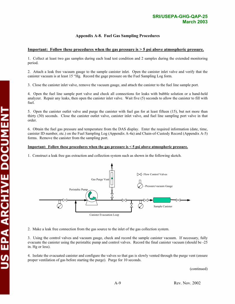
SRI/USEPA-GHG-QAP-25 March 2003
Appendix A-8. Fuel Gas Sampling Procedures
Important: Follow these procedures when the gas pressure is > 5 psi above atmospheric pressure.
1. Collect at least two gas samples during each load test condition and 2 samples during the extended monitoring period.
2. Attach a leak free vacuum gauge to the sample canister inlet. Open the canister inlet valve and verify that the canister vacuum is at least 15 “Hg. Record the gage pressure on the Fuel Sampling Log form.
3. Close the canister inlet valve, remove the vacuum gauge, and attach the canister to the fuel line sample port.
4. Open the fuel line sample port valve and check all connections for leaks with bubble solution or a hand-held analyzer. Repair any leaks, then open the canister inlet valve. Wait five (5) seconds to allow the canister to fill with fuel.
5. Open the canister outlet valve and purge the canister with fuel gas for at least fifteen (15), but not more than thirty (30) seconds. Close the canister outlet valve, canister inlet valve, and fuel line sampling port valve in that order.
6. Obtain the fuel gas pressure and temperature from the DAS display. Enter the required information (date, time, canister ID number, etc.) on the Fuel Sampling Log (Appendix A-4a) and Chain-of-Custody Record (Appendix A-5) forms. Remove the canister from the sampling port.
Important: Follow these procedures when the gas pressure is < 5 psi above atmospheric pressure.
1. Construct a leak free gas extraction and collection system such as shown in the following sketch.
Peristaltic Pump
Sample Canister
- Pressure/vacuum Gauge
- Flow Control Valves
Gas Purge Vent
Canister Evacuation Loop
2. Make a leak free connection from the gas source to the inlet of the gas collection system.
3. Using the control valves and vacuum gauge, check and record the sample canister vacuum. If necessary, fully evacuate the canister using the peristaltic pump and control valves. Record the final canister vacuum (should be -25 in. Hg or less).
4. Isolate the evacuated canister and configure the valves so that gas is slowly vented through the purge vent (ensure proper ventilation of gas before starting the purge). Purge for 10 seconds.
(continued)
A-9 Rev. Nov. 2002

SRI/USEPA-GHG-QAP-25 March 2003
Appendix A-8. Fuel Gas Sampling Procedures (continued)
5. Close the purge vent and slowly open the valves upstream of the canister and allow the canister to pressurize to no less than 2 psig.
6. With the pump still running, open the canister outlet valve and purge the canister for 5 seconds. Sequentially close the canister outlet valve, canister inlet valve, and pump inlet valve. Turn off pump.
7. Record the date, time, gas temperature (from DAS), canister ID number, and final canister pressure on log form (Appendix A-4b).
8. Return collected sample(s) to laboratory with completed chain-of-custody form (Appendix A-5).
A-10 Rev. Nov. 2002

SRI/USEPA-GHG-QAP-25 March 2003
Appendix A-9. Fuel Gas Sampling Log
Project ID: Location (city, state):
Date: Signature:
Unit Description: Fuel Source (e.g., pipeline, digester):
Note: If desired, assign random sample ID numbers to prevent the lab from attributing analysis results to a particular test or audit sample. Transfer sample ID numbers to Chain-of-Custody Record prior to sample shipment.
Obtain sample pressure and temperature from the DAS display.
Date Time Run ID Sample ID Canister ID
Initial Vacuum
(“Hg)
Fuel Pressure
(DAS)
Fuel Temperature
(DAS)
Notes:
A-11 Rev. Sept. 2002

SRI/USEPA-GHG-QAP-25 March 2003
Appendix A-10. Sample Chain-of-Custody Record
Southern Research Institute Chain-of-Custody Record
Important: Use separate Chain-of-Custody Record for each laboratory and/or sample type.
Project ID:
Originator’s signature:
Sample description & type (gas, liquid, other.):
Laboratory:
Address:
Location (city, state):
Unit description:
Phone: Fax:
City: State: Zip:
Sample ID Bottle/Canister ID Sample Pressure Sample Temp. (°F) Analyses Req’d
Relinquished by: Date: Time: Received by: Date: Time:
Relinquished by: Date: Time: Received by: Date: Time:
Relinquished by: Date: Time: Received by: Date: Time:
Notes: (shipper tracking #, other)
A-12 Rev. Sept. 2002

SRI/USEPA-GHG-QAP-25 March 2003
Appendix A-11. NOX Spiking and Calibration Data
Project ID: Location (city, state):
Date: Signature: 1. Perform immediately prior to starting short term testing. 2. Establish steady-state operations. 3. Observe CO and NOX analyzer charts until output is steady (i.e. < 0.5 % variation over 2 minutes). 4. Use the equations and sample tables below to calculate at least 9 different step changes (delta), spaced throughout the
anticipated CO and NOX analyzer spans, based on the calibration/spike gas concentrations. Enter the deltas in the table below.
5. At zero calibration/spike gas flow, note CO and NOX analyzer readings. Deltas will be zero. 6. Start the spike gas flow, adjust it to produce the desired CO step change (delta), and record the CO and NOX readings.
Perform three replications at each desired delta.
∆CO m1c CO spike
∆m2 = ,
CO1 − c CO spike ,
2a
2
a per ( ) g , 2 p g
NOX
Table 2. NO Delta for Given Spike Gas Flows Spike Flow, slm NO Delta
2.506 0.125 6.711 0.333 13.514 0.667 20.408 1.000 34.483 1.667
Assumes 1000 standard liter minute slmexhaust as flow 50 PPM NO in the s ike as.
analyzer span = 2.0 PPM ,∆ NOx
c NOx spike m2 =m1 + m2
Table 1. Spike Gas Flows for a Given CO Analyzer Delta a
CO Delta, PPM Spike Flow, slm 0.75 2.506
2 6.711 4 13.514 6 20.408
10 34.483 aAssumes 1000 standard liter per minute (slm) exhaust gas flow, 300 PPM CO in the spike gas. CO Analyzer span = 10 PPM
m2 = spike flow rate, slm m1 = exhaust gas flow rate; use 1000 slm ∆ = upscale increment (delta), PPM cspike = spike gas concentration, PPM
Calibration/Spike Gas Cyln. ID:_____________ CO PPM:___________ NO2 PPM:_______
Analyzer Spans (PPM) CO:________NOX :_________Op’r Rate: ________ Units:__________(kW, etc.)
Desired CO Delta Spike Flow, m2 (use m1 = 1000) Desired NOX Delta
Notes:
(continued)
A-13 Rev. Dec. 2002

SRI/USEPA-GHG-QAP-25 March 2003
Appendix A-11. NOX Spiking and Calibration Data (continued)
Time (24 hour) Desired CO Delta
Actual CO Delta, 1
Actual CO Delta, 2
Actual CO Delta, 3
Rotameter Flow (reference)
Time (24 hour) Desired NOX Delta
Actual NOX Delta, 1
Actual NOX Delta, 2
Actual NOX Delta, 3
Rotameter Flow (reference)
A-14 Rev. Dec. 2002
SRI/USEPA-GHG-QAP-25 March 2003
Appendix A-12. DAS Analog Channel Setup
Date: Job: DAS *.mdb Filename (include path):
Signature:
Channel Namea Unitsa Span
Analog Type
(mA or V)
Sensor/Transducer
Manufacturer Model Serial # Notes
1
2
3
4
5
6
7
8
9
10
11
12
13
14
15
16 a Enter this information into DAS Analog Tag Configuration form exactly as it appears here
A-15 Rev. Dec. 2002

SRI/USEPA-GHG-QAP-25 March 2003
Appendix A-13. DAS Calibration and Verification
Date: Job: Signature:
Note: 4 mA integer count is 3277; 20 mA integer count is 16383; -10 VDC integer count is -32768; +10 VDC integer count is 32767
Channel #, Desc, Units Calibration Inputs Verification
low mA/V
low integer
cnt.
low Eng. value high mA/V High integer
cnt. high Eng.
value DVM mA/V
DVM expected
value DAS value Measured
Value
% Diff. ([DAS-Measured]/Meas
ured)*100
A-16 Rev. Dec. 2002

SRI/USEPA-GHG-QAP-25 March 2003
Figure A-14. Corrective Action Report
Corrective Action Report
Verification Title:
Verification Description:
Description of Problem:
Originator: Date:
Investigation and Results:
Investigator: Date:
Corrective Action Taken:
Originator: Date: Approver: Date:
cc: GHG Center Project Manager, GHG Center Director, SRI QA Manager
A-17 Rev. Sept. 2002

SRI/USEPA-GHG-QAP-25 March 2003
Appendix A-15. Measurement Error Propagation
Each contributing measurement has uncertainty (or error) which propagates into the overall performance determination uncertainty. Absolute or relative errors compound differently, depending on the algebraic operation required for the overall determination (Skoog 1982). Absolute error is expressed in the units of measurement while relative error is a proportion or percent. Examples are: “980 ± 9.8 Btu (absolute error),” or “980 Btu ± 1.00 % (relative error).” In general, absolute errors compound for added or subtracted measurements while relative errors compound for multiplication and division.
For added or subtracted measurements:
2err abs c = err1 + err2 2 (Eqn. A-13.1) ,
errWhere:
c,abs = Compounded error, absolute err1 = Absolute error in first added (or subtracted) value err2 = Absolute error in second added (or subtracted) value
The relative error of the sum (or difference), then, is:
err abs c err rel c = , (Eqn. A-13.2) , value1 + value2
errWhere:
c,rel = Compounded error, relative value1 = First added value value2 = Second added value
The following table provides an example.
Compounded Uncertainty for Added (or Subtracted) Values Description Magnitude Absolute Error Relative Error (%)
Value 1 15 ± 0.80 ± 5.333 [(0.80/15)*100]
Value 2 2 ± 0.20 ± 10.000 [(0.20/2)*100]
Value 1 minus Value 2 13 ± 0.825 [(0.82+0.22)1/2]
± 5.497 [(0.825/13)*100]
For measurements which are multiplied or divided by each other, relative errors compound as follows:
2
err rel c = err1
2
+ err2
(Eqn. A-13.3) , value1 value2
A-18 Rev. Sept. 2002

SRI/USEPA-GHG-QAP-25 March 2003
errWhere:
c,rel = Compounded error, relative err1 = Error in first multiplied (or divided) value, absolute value err2 = Error in second multiplied (or divided) value, absolute value value1 = First multiplied (or divided) value value2 = Second multiplied (or divided) value
The following table provides an example.
Compounded Uncertainty for Multiplied (or Divided) Values Description Magnitude Relative Error (%) Absolute Error
Value 1 15 ± 5.333 ± 0.80 Value 2 2 ± 10.000 ± 0.20 Value 1 divided by Value 2 7.5 ± 11.333
[(0.053332+0.12)1/2] ± 0.85
[(11.333/7.5)*100]
Value 1 times Value 2 30 ± 11.333 [(0.053332+0.12)1/2]
± 3.40 [(11.333/30)*100]
Note that all errors can occur above or below the measured (or compounded) quantity. Analysts express the uncertainty as the result± the error and whether it is absolute or relative.
A-19 Rev. Sept. 2002