pml-16-c - becker & hickl · amplitude jitter of the single-photon pulses ... single-point...

High Performance

Photon Counting

PML-16-C

16 Channel Detector Head for

Time-Correlated

Single Photon Counting

User Manual

Becker & Hickl GmbH

PML-16C User Handbook 1

Becker & Hickl GmbH March 2006

High PerformancePhoton Counting

PML-16-C

16 Channel Detector Head for Time-CorrelatedSingle Photon Counting

User Handbook

Simultaneous detection in all 16 channels

Works with all bh TCSPC modules

Routing electronics and high voltage power supply included

Gain control and overload shutdown via bh DCC-100 detector controller card

1-by-16 arrangement of detector channels

IRF width 150 ps FWHM

Count rate up to 4 MHz

Tel. +49 / 30 / 787 56 32FAX +49 / 30 / 787 57 34http://www.becker-hickl.deemail: [email protected]

2 PML-16C User Handbook

Contents

Introduction............................................................................................................................ 3Principles of Multidetector TCSPC....................................................................................... 4Operating the PML-16C ........................................................................................................ 7

System Components and Cable Connections .................................................................... 7Status LEDs ....................................................................................................................... 8TCSPC Parameters ............................................................................................................ 8

System Parameters......................................................................................................... 8Trace and Display Parameters ....................................................................................... 9DCC-100 Parameters................................................................................................... 12Internal Discriminator Threshold of the PML-16C ..................................................... 13

Safety ............................................................................................................................... 13Technical Details of Single-Photon Detection .................................................................... 14

Amplitude Jitter of the Single-Photon Pulses.................................................................. 14Constant Fraction Triggering........................................................................................... 16

Adjusting the CFD Zero-Cross Level.......................................................................... 17Adjusting the Discriminator Threshold ....................................................................... 17

Channel Uniformity......................................................................................................... 19Efficiency................................................................................................................. 19Transit Time ............................................................................................................ 20

Spectral Response............................................................................................................ 20Background Count Rate................................................................................................... 21

Dark Count Rate ...................................................................................................... 21Afterpulsing ............................................................................................................. 22

PML-SPEC Assembly ......................................................................................................... 24MW-FLIM Multi-Wavelength FLIM Detection Systems.................................................... 26

One-Photon Excitation with Confocal Detection .................................................... 26Two-photon Excitation with Descanned Detection................................................. 26Two-photon Excitation with Non-Descanned Detection......................................... 27

Applications......................................................................................................................... 30Single-point tissue spectroscopy...................................................................................... 30Chlorophyll Transients .................................................................................................... 30Two-photon Laser Scanning Microscopy of Tissue ........................................................ 32

Troubleshooting................................................................................................................... 34Assistance through bh.......................................................................................................... 35Specification ........................................................................................................................ 36

Electrical .......................................................................................................................... 36Mechanical....................................................................................................................... 37

References............................................................................................................................ 38Index .................................................................................................................................... 39


IntroductionThe PML-16C detector is part of the Becker & Hickl modular multidimensional TCSPCsystems. The PML-16-C detects photons simultaneously in 16 channels of a multi-anodePMT. The module connects directly to the bh SPC-130, 140, 150, 630, 730, or 830 TCSPCdevices. Signal recording is based on bh’s proprietary multi-dimensional TCSPC technique [2,3, 10]. For each photon the internal routing electronics generate a timing pulse and a detectorchannel signal. These signals are used in the TCSPC device to build up the photon distributionover the arrival time of the photons and the detector channel number. The result is a set of 16waveform recordings for the 16 channels of the multi-anode PMT.

The required routing electronics and a high-voltage power supply for the multi-anode PMT isincluded in the PML-16-C module. The PML-16-C is controlled via the bh DCC-100 detectorcontroller [12]. The DCC-100 provides for the power supply, gain control, and overloadshutdown of the PML-16C.

Compared to sequential recording of 16 signals with a single detector the PML-16-C yields adramatically increased detection efficiency. Typical applications are optical tomography,multi-wavelength fluorescence lifetime microscopy, stopped flow experiments, and classicmulti-wavelength fluorescence lifetime experiments. The PML-16 is part of the bhPML-SPEC spectral detection system and the bh multi-wavelength FLIM systems [3].

This handbook covers the general function of the PML-16C, the interaction with the SPCmodule, the setting of the TCSPC system parameters, and the special technical issues ofphoton detection with multichannel PMTs. It describes the PML-SPEC spectral detection andMW-FLIM multi-wavelength FLIM detection systems and demonstrates the application ofthese systems to spectroscopy and imaging of biomedical systems. The basics of multi-dimensional TCSPC are described only briefly. For a comprehensive review of this techniqueplease refer to [2]. For detailed description of the bh SPC modules, the associated SPCMsoftware, applications of the bh TCSPC technique please refer to the bh TCSPC Handbook[3], available on www.becker-hickl.com.


Principles of Multidetector TCSPCClassic time-correlated single photon counting (TCSPC) is based on the detection of singlephotons of a periodic light signal, the measurement of the detection times within the signalperiod, and the reconstruction of the optical waveform from the individual time measurements[26]. Advanced TCSPC techniques are multi-dimensional. They measure not only the times ofthe photons after the excitation pulses but also the wavelength, the location of emission in asample, or the times from the start of the experiment [2, 3]. All TCSPC techniques make useof the fact that for low-level, high-repetition rate signals the light intensity is usually lowenough that the probability to detect more than one photon per signal period is negligible.Under this condition only one photon per signal period has considered. The photon isdetected, its parameters, i.e. time, wavelength, location, etc., are measured, and thedistribution of the photon density over these parameters is build up.

Compared with other time-resolved detection techniques TCSPC has a number of advantages,such as superior time resolution, near-ideal (or ‘shot-noise’ limited) sensitivity and signal-to-noise ratio, superior stability of the instrument response function [2, 3, 7], and multi-dimensionality. It is often objected against TCSPC that the count rate must be low enough tomake the detection of several photons per signal period unlikely. Often a limit of 0.01 photonsper signal period is given for TCSPC [26], but a detection rate up to 0.1 or even 0.2 per signalperiod can usually be tolerated [2, 3]. Thus, with modern excitation sources count rates on theorder of 10⋅106 s-1 can be obtained. Acquisition times at such count rates are in themillisecond range.

It is difficult to obtain count rates above 1⋅106 s-1 high from biological samples withoutcausing photobleaching or photodamage [6]. In other words, at typical count rates a singleTCSPC module with a single detector delivers undistorted waveforms.

Now consider an array of PMT channels over which the same photons flux is spread. Becauseit is unlikely that the complete array detects several photons per signal period it is alsounlikely that several channels of the array will detect a photon in one signal period. This is thebasic idea behind multi-detector TCSPC. Although several detectors are active simultaneouslythey are unlikely to detect a photon in the same signal period. The photon pulses delivered bythe detectors are therefore unlikely to overlap, and the times of the photons detected in alldetectors can be measured in a single TCSPC channel [2, 3, 9].

A block diagram of the PML-16-C is shown in Fig. 1.

’Channel’

Photon Pulses

Discriminators Encoder

’Disable count’

Detector number

to TCSPCmodule

.

.

D1

D16

..

.

.

..

AnodesDynodesPhoto-cathode

High

Multi-anode PMT Routing Electronics

....

Voltage

ENC

Fig. 1: Block diagram of the PML-16-C


The core of the PML-16 is a Hamamatsu R5900 16 channel multi-anode photomultiplier tubewith 16 separate output (anode) elements and a common cathode and dynode system [20, 22].The photon pulses from the individual anodes are fed into 16 discriminators, D1 through D16.When a photon is detected in any place of the photocathode the corresponding anode deliversa pulse which is detected by one of the discriminators. The discriminator output lines areconnected to a digital encoder, ENC. The encoder delivers four ‘channel’ bits and one ‘disablecount’ bit. The ‘channel’ bits represent the detector channel which detected the correspondingphoton. The ‘disable count’ bit is active when the encoding electronics was unable to providea valid ‘channel’ data word. This may happen is several PMT channels detected photonssimultaneously, or if the current single-photon pulse had an amplitude too small to be detectedby the discriminators.

The single-photon pulses of the photons of all detector channels are derived from the lastdynode of the R5900 PMT. The output from the dynode is positive. The pulses are amplifiedand inverted an a wide band amplifier, AMP. The single-photon pulses delivered by theamplifier are compatible with the CFD inputs of the bh TCSPC modules.

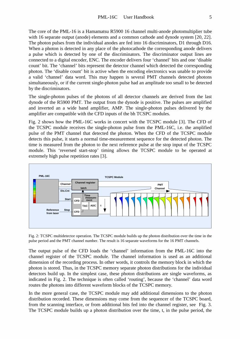
Fig. 2 shows how the PML-16C works in concert with the TCSPC module [3]. The CFD ofthe TCSPC module receives the single-photon pulse from the PML-16C, i.e. the amplifiedpulse of the PMT channel that detected the photon. When the CFD of the TCSPC moduledetects this pulse, it starts a normal time-measurement sequence for the detected photon. Thetime is measured from the photon to the next reference pulse at the stop input of the TCSPCmodule. This ‘reversed start-stop’ timing allows the TCSPC module to be operated atextremely high pulse repetition rates [3].

measure-Start

Stop

CFD

CFDfrom laser

Time

t

Channel register

Reference

latch

ment

ADCTAC

Channel

Channel Dis.Cnt

PMT

TCSPC ModulePML-16C

Fig. 2: TCSPC multidetector operation. The TCSPC module builds up the photon distribution over the time in thepulse period and the PMT channel number. The result is 16 separate waveforms for the 16 PMT channels.

The output pulse of the CFD loads the ‘channel’ information from the PML-16C into thechannel register of the TCSPC module. The channel information is used as an additionaldimension of the recording process. In other words, it controls the memory block in which thephoton is stored. Thus, in the TCSPC memory separate photon distributions for the individualdetectors build up. In the simplest case, these photon distributions are single waveforms, asindicated in Fig. 2. The technique is often called ‘routing’, because the ‘channel’ data wordroutes the photons into different waveform blocks of the TCSPC memory.

In the more general case, the TCSPC module may add additional dimensions to the photondistribution recorded. These dimensions may come from the sequencer of the TCSPC board,from the scanning interface, or from additional bits fed into the channel register, see Fig. 3.The TCSPC module builds up a photon distribution over the time, t, in the pulse period, the


detector channel number, the time from the start of the experiment, T, the coordinates of ascanning area, X and Y, and over the information provided by an additional channel data wordused to multiplex several lasers or sample positions. Please see [3] for details.

Due to the high count rates applicable with the bh SPC modules there is a non-zero probabilityto detect more than one photon within the response time of the amplifier/comparator circuitryin the PML-16C. Furthermore, it may happen that the CFD of the SPC detects a photon pulsewhich was too small to be detected by the PML routing circuitry. In such cases the‘disable count' bit suppresses the recording of the misrouted event in the TCSPC module.

measure-Start

Stop

CFD

CFDfrom laser

Time

t

Channel register

Experiment

Scan Clocksetc.

Trigger

Reference

Sequencer,

latch

ment

ADCTAC

Channel PMT Channel

Photondistribution

PMT

Photondistribution

Photondistribution

T, X, Y, etc.

Dis.Cnt

............

PML-16C

channel 1PMT

channel 2PMT

channel 16

scanninginterface

Multiplexing Multiplexing channel

Fig. 3: Multidetector operation of a multi-dimensional TCSPC system. The TCSPC module builds up a photondistribution over the time in the pulse period, the detector channel number, the time from the start of theexperiment, the coordinates of a scanning area, and over the information provided by an additional channel dataword.

Interestingly, multi-channel detection reduces classic pile-up effects. If several photons arrivewithin one signal period they are likely to hit the detector in different channels. The‘disable count' bit then suppresses the recording of both photons thus avoiding signaldistortion by the loss of only the second photon [2, 3].


Operating the PML-16C

System Components and Cable Connections

The system components and cable connections for operating a PML-16C in a TCSPC systemare shown in Fig. 4. The 15 pin sub-D connector of the PML-16C is connected both to theTCSPC module [3] and the DCC-100 detector controller [12]. The TCSPC module can be anyof the bh SPC-630, 730, 830, 140/144 or 150/154 modules.

’SYNC’

’CFD’

SPC module

DCC-100

Routing

Power supply

PML-16C

fromLaser

C1

C2

C3

see (1)

(1) cable length:<1.5m for SPC-630, 730, 830, 1407m for SPC-130

Photonpulses

Fig. 4: Cable connections between the PML-16C, the DCC-100 and the TCSPC module.

The routing signals (the ‘channel’ bits) are connected to the routing input connector of theSPC module. For modules with two connectors (such as the SPC-830) the routing connector isthe lower one, i.e. the one closer to the motherboard of the computer. The photon pulses of thePML-16C are connected to the ‘CFD’ input of the SPC modules. A 50-Ω SMA cable is usedfor this connection. Except for the SPC-130/134 the photon pulse cable should not be longerthan the routing cable in order to maintain correct sampling of the routing bits by the channelregister of the SPC module.

The bh SPC-130 modules and the SPC-134 packages were originally designed formultiplexing, not for multi-detector operation. Therefore the SPC-130 cards do not have anadjustable latch delay to read the routing signals from a multichannel detector head.Nevertheless, SPC-130 modules manufactured later than January 2004 can be used with thePML-16C. To provide for the correct latch delay the photon pulses from the PML must bedelayed by about 35 ns. This can be achieved by using a 7 m cable in the photon pulse linefrom the PML to the SPC-130, see Fig. 4.

The older SPC-330, 430, 530 work with the PML-16C in the same way as the SPC-630, 730and 830. However, these modules have an ISA connector. Because a DCC-100 card is used tocontrol the PML-16C operation with the older SPC modules requires a computer that has bothISA and PCI slots.

Unlike its predecessor, the PML-16 [13], the PML-16C does not require any external high-voltage power supply. The high voltage for the PMT tube is generated internally. The voltage,i.e. the PMT gain, is controlled via a DCC-100 detector controller card. The DCC-100 alsodelivers the +5V, -5V, and +12V power supply to the PML-16. The PML-16C can beconnected both to ‘Connector 1’ and to ‘Connector 3’ of the DCC-100.


If the maximum output current of the PMT is exceeded the DCC-100 automatically shutsdown the high voltage. This overload protection mechanism normally prevents the PMT frombeing destroyed. Nevertheless, overload shutdown should be considered an emergency and notbe used to switch off the detector in standard situations.

Status LEDs

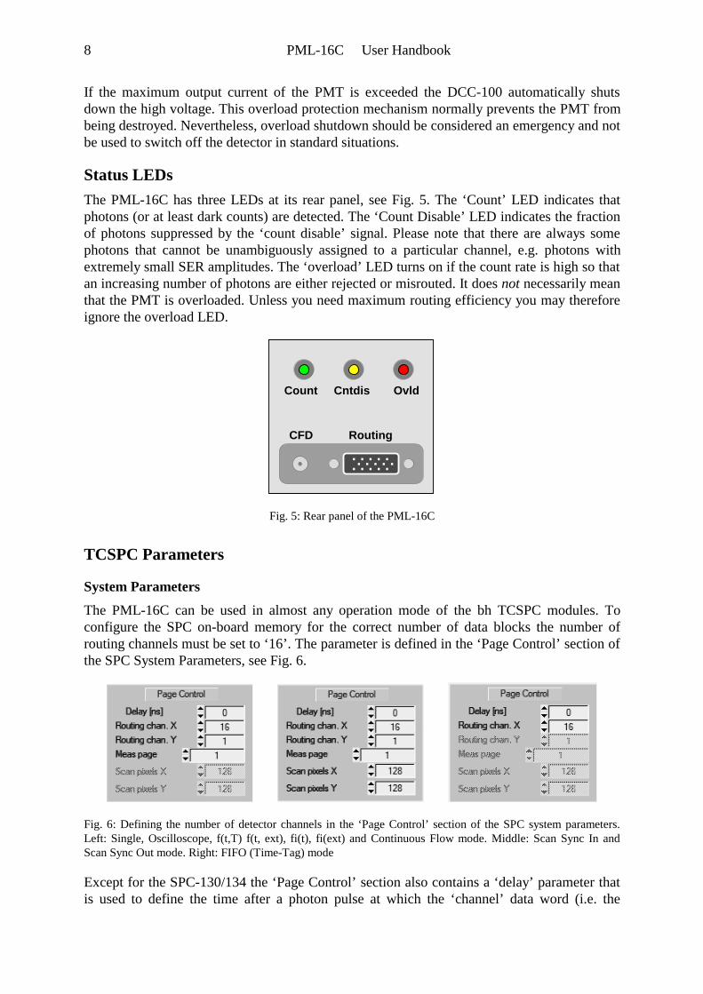
The PML-16C has three LEDs at its rear panel, see Fig. 5. The ‘Count’ LED indicates thatphotons (or at least dark counts) are detected. The ‘Count Disable’ LED indicates the fractionof photons suppressed by the ‘count disable’ signal. Please note that there are always somephotons that cannot be unambiguously assigned to a particular channel, e.g. photons withextremely small SER amplitudes. The ‘overload’ LED turns on if the count rate is high so thatan increasing number of photons are either rejected or misrouted. It does not necessarily meanthat the PMT is overloaded. Unless you need maximum routing efficiency you may thereforeignore the overload LED.

Count Cntdis Ovld

RoutingCFD

. . . . .. . . . .. . . . .

Fig. 5: Rear panel of the PML-16C

TCSPC Parameters

System Parameters

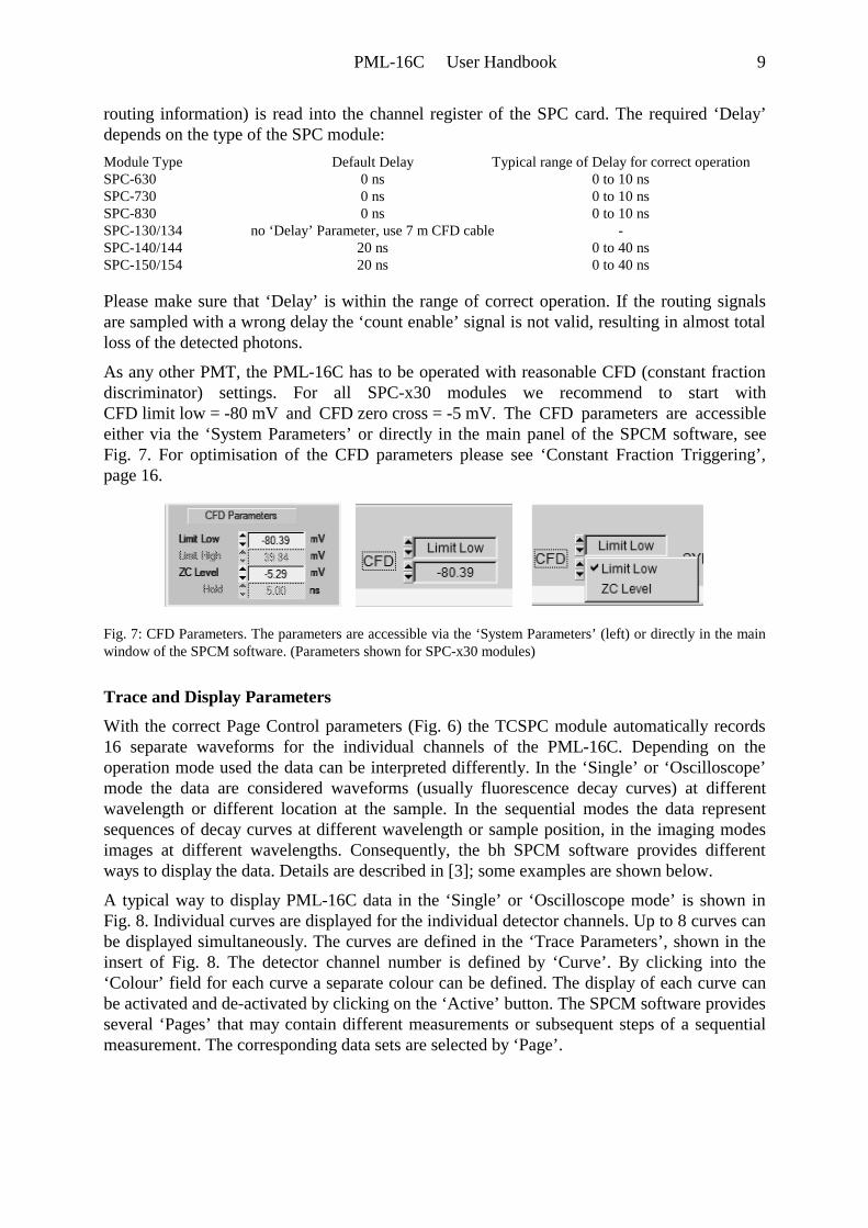
The PML-16C can be used in almost any operation mode of the bh TCSPC modules. Toconfigure the SPC on-board memory for the correct number of data blocks the number ofrouting channels must be set to ‘16’. The parameter is defined in the ‘Page Control’ section ofthe SPC System Parameters, see Fig. 6.

Fig. 6: Defining the number of detector channels in the ‘Page Control’ section of the SPC system parameters.Left: Single, Oscilloscope, f(t,T) f(t, ext), fi(t), fi(ext) and Continuous Flow mode. Middle: Scan Sync In andScan Sync Out mode. Right: FIFO (Time-Tag) mode

Except for the SPC-130/134 the ‘Page Control’ section also contains a ‘delay’ parameter thatis used to define the time after a photon pulse at which the ‘channel’ data word (i.e. the


routing information) is read into the channel register of the SPC card. The required ‘Delay’depends on the type of the SPC module:

Module Type Default Delay Typical range of Delay for correct operationSPC-630 0 ns 0 to 10 nsSPC-730 0 ns 0 to 10 nsSPC-830 0 ns 0 to 10 nsSPC-130/134 no ‘Delay’ Parameter, use 7 m CFD cable -SPC-140/144 20 ns 0 to 40 nsSPC-150/154 20 ns 0 to 40 ns

Please make sure that ‘Delay’ is within the range of correct operation. If the routing signalsare sampled with a wrong delay the ‘count enable’ signal is not valid, resulting in almost totalloss of the detected photons.

As any other PMT, the PML-16C has to be operated with reasonable CFD (constant fractiondiscriminator) settings. For all SPC-x30 modules we recommend to start withCFD limit low = -80 mV and CFD zero cross = -5 mV. The CFD parameters are accessibleeither via the ‘System Parameters’ or directly in the main panel of the SPCM software, seeFig. 7. For optimisation of the CFD parameters please see ‘Constant Fraction Triggering’,page 16.

Fig. 7: CFD Parameters. The parameters are accessible via the ‘System Parameters’ (left) or directly in the mainwindow of the SPCM software. (Parameters shown for SPC-x30 modules)

Trace and Display Parameters

With the correct Page Control parameters (Fig. 6) the TCSPC module automatically records16 separate waveforms for the individual channels of the PML-16C. Depending on theoperation mode used the data can be interpreted differently. In the ‘Single’ or ‘Oscilloscope’mode the data are considered waveforms (usually fluorescence decay curves) at differentwavelength or different location at the sample. In the sequential modes the data representsequences of decay curves at different wavelength or sample position, in the imaging modesimages at different wavelengths. Consequently, the bh SPCM software provides differentways to display the data. Details are described in [3]; some examples are shown below.

A typical way to display PML-16C data in the ‘Single’ or ‘Oscilloscope mode’ is shown inFig. 8. Individual curves are displayed for the individual detector channels. Up to 8 curves canbe displayed simultaneously. The curves are defined in the ‘Trace Parameters’, shown in theinsert of Fig. 8. The detector channel number is defined by ‘Curve’. By clicking into the‘Colour’ field for each curve a separate colour can be defined. The display of each curve canbe activated and de-activated by clicking on the ‘Active’ button. The SPCM software providesseveral ‘Pages’ that may contain different measurements or subsequent steps of a sequentialmeasurement. The corresponding data sets are selected by ‘Page’.


Fig. 8: Display of PML-16C data in the ‘Single’ or ‘Oscilloscope’ mode. Individual curves are displayed for theindividual detector channels. The curves are defined in the ‘Display’ parameters of the SPCM software (seeinsert).

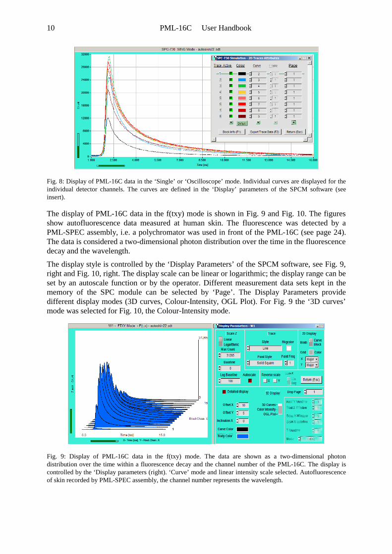
The display of PML-16C data in the f(txy) mode is shown in Fig. 9 and Fig. 10. The figuresshow autofluorescence data measured at human skin. The fluorescence was detected by aPML-SPEC assembly, i.e. a polychromator was used in front of the PML-16C (see page 24).The data is considered a two-dimensional photon distribution over the time in the fluorescencedecay and the wavelength.

The display style is controlled by the ‘Display Parameters’ of the SPCM software, see Fig. 9,right and Fig. 10, right. The display scale can be linear or logarithmic; the display range can beset by an autoscale function or by the operator. Different measurement data sets kept in thememory of the SPC module can be selected by ‘Page’. The Display Parameters providedifferent display modes (3D curves, Colour-Intensity, OGL Plot). For Fig. 9 the ‘3D curves’mode was selected for Fig. 10, the Colour-Intensity mode.

Fig. 9: Display of PML-16C data in the f(txy) mode. The data are shown as a two-dimensional photondistribution over the time within a fluorescence decay and the channel number of the PML-16C. The display iscontrolled by the ‘Display parameters (right). ‘Curve’ mode and linear intensity scale selected. Autofluorescenceof skin recorded by PML-SPEC assembly, the channel number represents the wavelength.


Fig. 10: Display of PML-16C data in the f(txy) mode. The data are shown as a three-dimensional photondistribution over the time within a fluorescence decay and the channel number of the PML-16C. The display iscontrolled by the ‘Display parameters (right). ‘Colour-Intensity’ mode and linear intensity scale selected.Autofluorescence of skin recorded by PML-SPEC assembly. The channel number represents the wavelength.

Please note that the data structures in the ‘Single’, ‘Oscilloscope’, and ‘f(t,x,y)’ modes areidentical. Therefore you may run a measurement in the ‘Single’ mode and display the data inthe ‘f(t, x, y)’ mode or vice versa.

An example of a ‘Scan Sync In’ mode measurement is shown in Fig. 11. The images weretaken in a Zeiss LSM 510 NLO two-photon laser scanning microscope upgraded with a bhSPC-830 TCSPC module and a bh MW-FLIM assembly. The sample was an unstained mousekidney section. Eight display windows were defined showing the integral fluorescence of thesample in eight wavelength intervals. Each image has its own display parameters. Theparameters of the left image of the second row are shown right.

Fig. 11: Multi-wavelength measurement in the ‘Scan Sync In’ mode. LSM 510 two-photon laser scanningmicroscope, SPC-830 TCSPC module, bh MW-FLIM assembly. The sample is a mouse kidney section. Imagesin different wavelength intervals are shown left. Each image has its own display parameters; the parameters of theleft image of the second row are shown right.

The display mode is the ‘Colour Intensity’ mode. The colours are defined in the lower left ofthe display parameter panel. They were selected according to the true colour of the wavelengthintervals. The wavelength intervals themselves are defined in the ‘Window Parameters’ of theSPCM software (not shown here). The defined wavelength intervals are assigned to thecurrent image by ‘Routing X Window’, in the lower right of the display parameter panel.Images can also be displayed in time-windows specified in the ‘Window Parameters’. Thewindow for the current image is selected under ‘T Window’, in the lower right of the panel.


For details of the display functions please see [3]; for fluorescence lifetime analysis of theimages please see [15].

DCC-100 Parameters

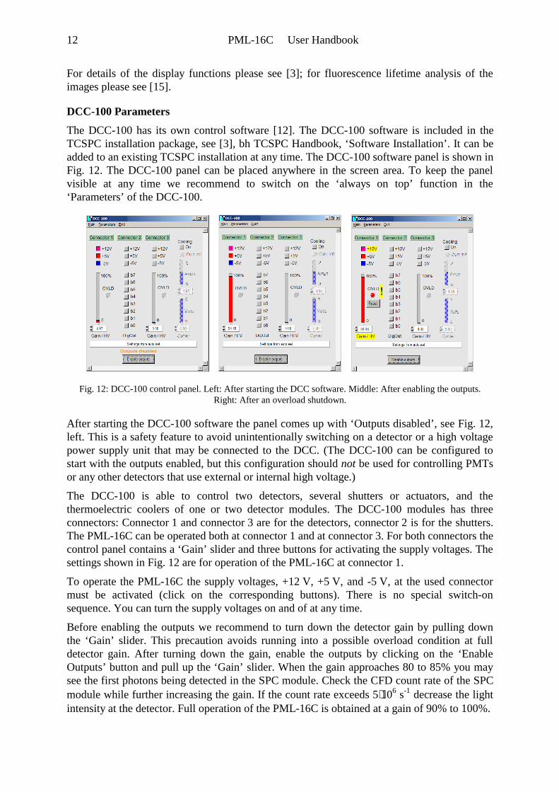
The DCC-100 has its own control software [12]. The DCC-100 software is included in theTCSPC installation package, see [3], bh TCSPC Handbook, ‘Software Installation’. It can beadded to an existing TCSPC installation at any time. The DCC-100 software panel is shown inFig. 12. The DCC-100 panel can be placed anywhere in the screen area. To keep the panelvisible at any time we recommend to switch on the ‘always on top’ function in the‘Parameters’ of the DCC-100.

Fig. 12: DCC-100 control panel. Left: After starting the DCC software. Middle: After enabling the outputs.Right: After an overload shutdown.

After starting the DCC-100 software the panel comes up with ‘Outputs disabled’, see Fig. 12,left. This is a safety feature to avoid unintentionally switching on a detector or a high voltagepower supply unit that may be connected to the DCC. (The DCC-100 can be configured tostart with the outputs enabled, but this configuration should not be used for controlling PMTsor any other detectors that use external or internal high voltage.)

The DCC-100 is able to control two detectors, several shutters or actuators, and thethermoelectric coolers of one or two detector modules. The DCC-100 modules has threeconnectors: Connector 1 and connector 3 are for the detectors, connector 2 is for the shutters.The PML-16C can be operated both at connector 1 and at connector 3. For both connectors thecontrol panel contains a ‘Gain’ slider and three buttons for activating the supply voltages. Thesettings shown in Fig. 12 are for operation of the PML-16C at connector 1.

To operate the PML-16C the supply voltages, +12 V, +5 V, and -5 V, at the used connectormust be activated (click on the corresponding buttons). There is no special switch-onsequence. You can turn the supply voltages on and of at any time.

Before enabling the outputs we recommend to turn down the detector gain by pulling downthe ‘Gain’ slider. This precaution avoids running into a possible overload condition at fulldetector gain. After turning down the gain, enable the outputs by clicking on the ‘EnableOutputs’ button and pull up the ‘Gain’ slider. When the gain approaches 80 to 85% you maysee the first photons being detected in the SPC module. Check the CFD count rate of the SPCmodule while further increasing the gain. If the count rate exceeds 5⋅106 s-1 decrease the lightintensity at the detector. Full operation of the PML-16C is obtained at a gain of 90% to 100%.


The ‘Gain’ slider controls the operating voltage of the PMT. The actual gain of a PMTincreases with approximately the 4th power of the operating voltage.

Please note:

Photon counting records the pulses the detector delivers for the individual photons of the lightsignal. The detector gain determines the amplitude of these pulses, not their frequency. Thedetector gain can therefore not be used to control the magnitude of the recorded photondistributions. Any attempt to decrease the sensitivity by reducing the detector gain results indecreased signal-to-noise ratio and poor channel uniformity (see ‘Technical Details of Single-Photon Detection’, page 14).

If the light intensity at the PML-16C is too high the DCC-100 shuts down the gain and the+12 V supply voltage. In extreme cases this may happen at a gain far below the single-photondetection level, i.e. before the SPC module displays a CFD count rate. The DCC-100 panelafter an overload shutdown is shown in Fig. 12, right. If an overload shutdown has occurred,remove the source of the overload. Then click on the ‘Reset’ button. After the reset thePML-16 resumes normal operation. Please do not attempt to avoid overload by operating thePML-16C at reduced detector gain. This would result in poor counting efficiency and poorchannel uniformity, see Fig. 21.

Internal Discriminator Threshold of the PML-16C

The PML-16C has 16 internal discriminators to generate the routing information (see Fig. 1,page 4). The threshold of these discriminators can be adjusted by a trimpot. The internalthreshold is factory adjusted. Changing the threshold is not normally needed and thereforediscouraged. If the threshold has been changed for any reasons it can be re-adjusted asdescribed below.

Run a measurement in the oscilloscope mode of the SPC module. Use the stop option ‘Stop T’and a collection time of about 1 second. Activate the ‘Trace Statistics’ panel. Activate thePML-16C but do not send light into the PML-16C. Turn the threshold potentiometer left untilthe ‘Overload’ LED at the back of the PML-16C turns on. The threshold is then close to zero.Then turn the potentiometer back (toward higher threshold) until the overload LED turns off.

Send defined light signals to the PML-16C. Adjust the internal threshold in order to obtain amaximum of the ‘total counts’, good channel separation and good channel uniformity. Thefinal settings may be slightly above, but not far from the point where the overload LED turnsoff.

Safety

The R5900 PMT of PML-16C is operated at a cathode voltage of up to 1000 V. The cathodevoltage is generated by a DC-DC converter inside the PML-16C. Therefore do not open thehousing of the PML-16C when the 15 pin cables from the DCC-100 and the SPC module areconnected. Moreover, please operate the PML-16 only with the correct routing and powersupply cables. Make sure that the cables are connected to the correct connectors of theDCC-100 and the SPC module. Using wrong cables or connecting the cables to a wrongconnector (e.g. a monitor output from a display card) can seriously damage the PML-16C, theDCC-100, the SPC module or the display card. Make sure not to connect a computer monitorto one of the 15 pin connectors of the DCC-100 of the SPC card. Please do not disconnect anycables when the PML-16C is in operation.


Technical Details of Single-Photon DetectionIn early times of TCSPC users were confused by countless and often contradicting instructionsabout optimising the PMTs of their instruments, configuring constant fraction discriminators,tweaking discriminator thresholds, trigger fractions, and preamplifier bandwidth or gain. Thedifficulties in part resulted from the slow speed of the early TCSPC electronics and therelatively slow rise times of the single-electron response of the PMTs used. Other advice, suchas reducing the relative dark count rate by increasing the CFD threshold, resulted from poorlyperforming PMTs and preamplifiers or was plainly wrong. Confusion resulted also fromapplying timing solutions optimised for high-energy particle detection by scintillatorsstraightforward to single-photon detection.

With the currently available high speed constant-fraction discriminators, low-noisepreamplifiers, and fast PMTs, adjustments, if required at all, are largely simplified. In fact, alla TCSPC user has to do is to set a discriminator threshold above the noise level of thepreamplifier and to increase the operating voltage of the PMT until the counting efficiencystarts to saturate.

Nevertheless, the technical details of operating a multichannel PMT in a TCSPC system aredescribed in the following paragraphs. The examples given in this sections are recorded withtypical devices. The PMT gain and CFD parameters given are considered representative.Please note, however, that individual PMTs may slightly differ in gain, efficiency, and spectralresponse.

Amplitude Jitter of the Single-Photon Pulses

A conventional photomultiplier tube (PMT) is a vacuum device which contains aphotocathode, a number of dynodes (amplifying stages) and an anode which delivers theoutput signal [2, 3, 22]. The principle is shown in Fig. 13.

CathodeD1

D2 D3

D4 D5

D6 D7

D8 AnodePhoto-

Fig. 13: Principle of a conventional PMT

The operating voltage builds up an electrical field that accelerates the electrons from thephotocathode to the first dynode D1, further to the next dynodes, and from D8 to the anode.When a photoelectron hits D1 it releases several secondary electrons. The same happens forthe electrons emitted by D1 when they hit D2. The overall gain reaches values of 106 to 108.The secondary emission at the dynodes is very fast; therefore the secondary electrons resultingfrom one photoelectron arrive at the anode within a few ns. Due to the high gain and the shortresponse a single photoelectron yields an easily detectable current pulse at the anode.

The detector output pulse for a single photon, (or a single photoelectron) is called the ‘SingleElectron Response’ or ‘SER’. Due to the random nature of the secondary emission, the pulseamplitude varies from pulse to pulse. The secondary emission coefficient at the dynodes is ofthe order of 5 to 10, resulting in a variation of the number of secondary electrons on the orderof 1:2 to 1:4. Moreover, some of the primary electrons are scattered without anymultiplication, which further increases the effective width of the amplitude distribution.


The single-photon (SER) pulses of a PML-16C detector are shown in Fig. 14. The pulses havea rise time of about 600 ps and a width of about 2 ns.

Fig. 14: Single-photon pulses delivered by the PML-16C. Gain = 95%, recorded with Tektronix ??? oscilloscope.Horizontal 2 ns / div, vertical 20 mV / div.

The amplitude of the pulses varies over a wide range. The pulse amplitude distributionmeasured at three different channels of the same PML-16C is shown in Fig. 15.

Fig. 15: Amplitude distribution of the single-photon pulses of a PML-16C. Channel 1 (blue), channel 4 (green)and channel 16 (red). DCC gain setting 95%, corresponding to a cathode voltage of -950 V.

Fig. 15 shows that the width at half maximum of the amplitude distribution is 1:3 to 1:4. Thepulse amplitude distribution consists of three major components. The largest part of thedistribution, above about 1 unit, is due to the regular single-photon pulses. It also containsbackground pulses due to thermal emission at the photocathode. The amplitude distribution isslightly different for different channels, which has to be taken into regard when the CFDthreshold is optimised (see Fig. 21).

Especially at high gain there is usually a sub-structure in the amplitude distribution. It isprobably caused by spatial nonuniformity in the secondary emission coefficient, and by thediscrete number of secondary electrons emitted at the first dynode.

Thermal emission, photoelectron emission, and reflection of primary electrons at the dynodescause an increase of the pulse density at low amplitudes. At very low amplitudes electronic


noise, either from the preamplifier or from the environment, causes a third peak of extremelyhigh count rate.

The amplitude jitter of the SER pulses sets two general requirements to the inputdiscriminator circuitry in the TCSPC module. On the one hand, the trigger delay must beindependent of the variable amplitude of the pulses. On the other hand, the discriminatorthreshold must be high enough to reject the electronic noise and the pulses caused by thermalemission in later stages of the dynode chain of the PMT.

Constant Fraction Triggering

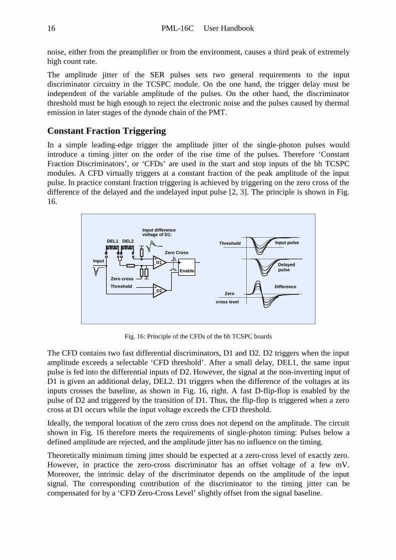
In a simple leading-edge trigger the amplitude jitter of the single-photon pulses wouldintroduce a timing jitter on the order of the rise time of the pulses. Therefore ‘ConstantFraction Discriminators’, or ‘CFDs’ are used in the start and stop inputs of the bh TCSPCmodules. A CFD virtually triggers at a constant fraction of the peak amplitude of the inputpulse. In practice constant fraction triggering is achieved by triggering on the zero cross of thedifference of the delayed and the undelayed input pulse [2, 3]. The principle is shown in Fig.16.

Zero cross

DEL1

+-

Input differencevoltage of D1:

DEL2

+-

Threshold

Input D1

D2

Zero Cross

Enable

Input pulse

Difference

Threshold

Zero

cross level

Delayedpulse

Fig. 16: Principle of the CFDs of the bh TCSPC boards

The CFD contains two fast differential discriminators, D1 and D2. D2 triggers when the inputamplitude exceeds a selectable ‘CFD threshold’. After a small delay, DEL1, the same inputpulse is fed into the differential inputs of D2. However, the signal at the non-inverting input ofD1 is given an additional delay, DEL2. D1 triggers when the difference of the voltages at itsinputs crosses the baseline, as shown in Fig. 16, right. A fast D-flip-flop is enabled by thepulse of D2 and triggered by the transition of D1. Thus, the flip-flop is triggered when a zerocross at D1 occurs while the input voltage exceeds the CFD threshold.

Ideally, the temporal location of the zero cross does not depend on the amplitude. The circuitshown in Fig. 16 therefore meets the requirements of single-photon timing: Pulses below adefined amplitude are rejected, and the amplitude jitter has no influence on the timing.

Theoretically minimum timing jitter should be expected at a zero-cross level of exactly zero.However, in practice the zero-cross discriminator has an offset voltage of a few mV.Moreover, the intrinsic delay of the discriminator depends on the amplitude of the inputsignal. The corresponding contribution of the discriminator to the timing jitter can becompensated for by a ‘CFD Zero-Cross Level’ slightly offset from the signal baseline.


Adjusting the CFD Zero-Cross Level

The dependence of the instrument response function (IRF) of one channel of a PML-16C onthe zero-cross level is shown in Fig. 17. Due to the fast discriminators used in the CFDs of thebh TCSPC modules the influence of the zero-cross level on the IRF is small. A reasonableIRF is obtained within a range of +30 mV to -30 mV, best results within +10 mV to -10 mV.The adjustment of the zero cross is therefore not critical, or, in many cases, even notnecessary.

Fig. 17: Dependence of the IRF of a single PML-16C channel on the CFD Zero-Cross Level. Black +30 mV,green +10 mV, red -10 mV, magenta -30 mV. The FWHM of the IRF is shown in the inserts. Left: Linear scale,200 ps / division, 1.22 ps / point. Right: Logarithmic scale, 500 ps / division, 1.22 ps / point. Light pulses fromBHL-600 diode laser, pulse width 30 ps, repetition rate 50 MHz.

Zero-cross levels closer than 5mV to the signal baseline should be avoided. In that case, thezero-cross discriminator may trigger due to spurious signals from the synchronisation channelor may even oscillate. Of course, spurious triggering and oscillation stop when an input pulsearrives, but some after-ringing may still be present and modulate the trigger delay. The resultcan be poor differential nonlinearity (ripple in the recorded curves) or a double structure in theIRF.

Adjusting the Discriminator Threshold

A TCSPC system should record the regular photon pulses, but not the thermal dynode pulsesand the electronic noise background. Therefore, the optimum CFD threshold is near the valleybetween the regular photon pulse distribution and the peak caused by electronic noise anddynode emission, see Fig. 18, left. The pulse amplitude distribution stretches horizontally withincreasing PMT gain. Therefore the optimum CFD threshold increases with the PMT gain.


Pulse amplitude CFD Threshold

Count

Rate

Pulses

per

second

Amplitude distribution

regular photon

electronic noise

pulses from dynodes

electronic noise

pulses from dynodes

regular photon pulses

Optimum Thres.Optimumthreshold

Rate vs. threshold

pulses

Gain 2

Gain1 Gain 2

Gain1

PMT Gain

Count

Rate Optimum Gain

Rate vs. PMT gain

Threshold 1

Threshold 2

1 2

1 21 2

Fig. 18: Left: General shape of the amplitude distribution of the single-photon pulses. Middle: Dependence of thecount rate on the CFD threshold. Right: Dependence of the count rate on the PMT gain.

The corresponding dependence of the count rate on the discriminator threshold is shown inFig. 18, middle. The PMT is illuminated with light of low intensity. When the discriminatorthreshold (‘CFD limit Low’) is decreased the count rate increases. At a sufficiently lowthreshold the increase of the count rate flattens, and in the ideal case forms a plateau. ThePML-16C-0 and -1 detectors the counting plateau is clearly visible. For other PMTs theplateau may be not very pronounced. However, at least a flattening of the count rate increaseshould be found.

At very low threshold the count rate increases again because thermal dynode pulses orelectronic noise are detected. In practice the dynode peak may be not very prominent or evenbe hidden in the electronic noise.

A similar behaviour is found if the gain of the PMT is changed, see Fig. 18, right. The countrate increases with increasing gain and eventually reaches a plateau.

Consequently, there are two ways to find a reasonable operating point of the PMT: You mayeither set a reasonable PMT gain and vary the CFD threshold, or set a reasonable CFDthreshold and vary the PMT gain. For the PML-16C the DCC gain should be between 90 and95 %, corresponding to a PMT operating voltage between 900 and 950 V. The CFD thresholdshould be within a range of -50 to -100 mV.

The CFD threshold, does, of course also influence the shape of the IRF. An example is givenin Fig. 19. The CFD threshold was increased in 20 mV steps from -20 mV to -140 mV. Atvery low threshold (-20 mV and -40 mV) the IRF develops a shoulder prior to the mean peak.The shoulder is typical of front-window PMTs operated at low threshold. Most likely, it iscaused by photoelectron emission at the first dynode. A clean IRF at good efficiency isobtained for thresholds from -60 mV to -100 mV. The efficiency drops noticeably at -120 mVand -140 mV. Despite of the short IRF width (see inserts in Fig. 19) operating the PML-16Cin this threshold range is discouraged. The high threshold not only results in loss of photonsbut also in large efficiency differences between the channels (see paragraph below).


Fig. 19: IRF for CFD thresholds from -20 mV to -140 mV. The FWHM of the IRF is shown in the insert. Left:Linear scale, 200 ps / division, 1.22 ps / point. Right: Logarithmic scale, 500 ps / division, 1.22 ps / point. Lightpulses from BHL-600 diode laser, pulse width 30 ps, repetition rate 50 MHz.

Channel Uniformity

Efficiency

For a multichannel PMT the CFD threshold has also a noticeable influence on the uniformityof the channels in terms of efficiency. Although all PMT channels use the same dynodesystem and the same operating voltage the pulse amplitude distribution for the individualchannels may differ noticeably (see Fig. 15). The situation is illustrated in Fig. 20. PMTchannel B has a gain 25% lower than channel A. Threshold 2 yields a satisfactory efficiencyfor channel A, but not for channel B. If this threshold is used the result is an large variation inthe efficiency of the channels. Better results are obtained with threshold 1. Both channels arethen in the ‘counting plateau’, and the gain difference has little influence on the efficiency.For the PML-16C it is therefore important to set the PMT gain high enough for the CFDthreshold used (or the CFD threshold low enough for the gain used) to obtain reasonablecounting efficiency for the channel of the lowest gain.

CFD Threshold

Count

Rate

Threshold 1 Threshold 2

Channel A

Channel B

Fig. 20: Effect of gain variations of the PMT channels

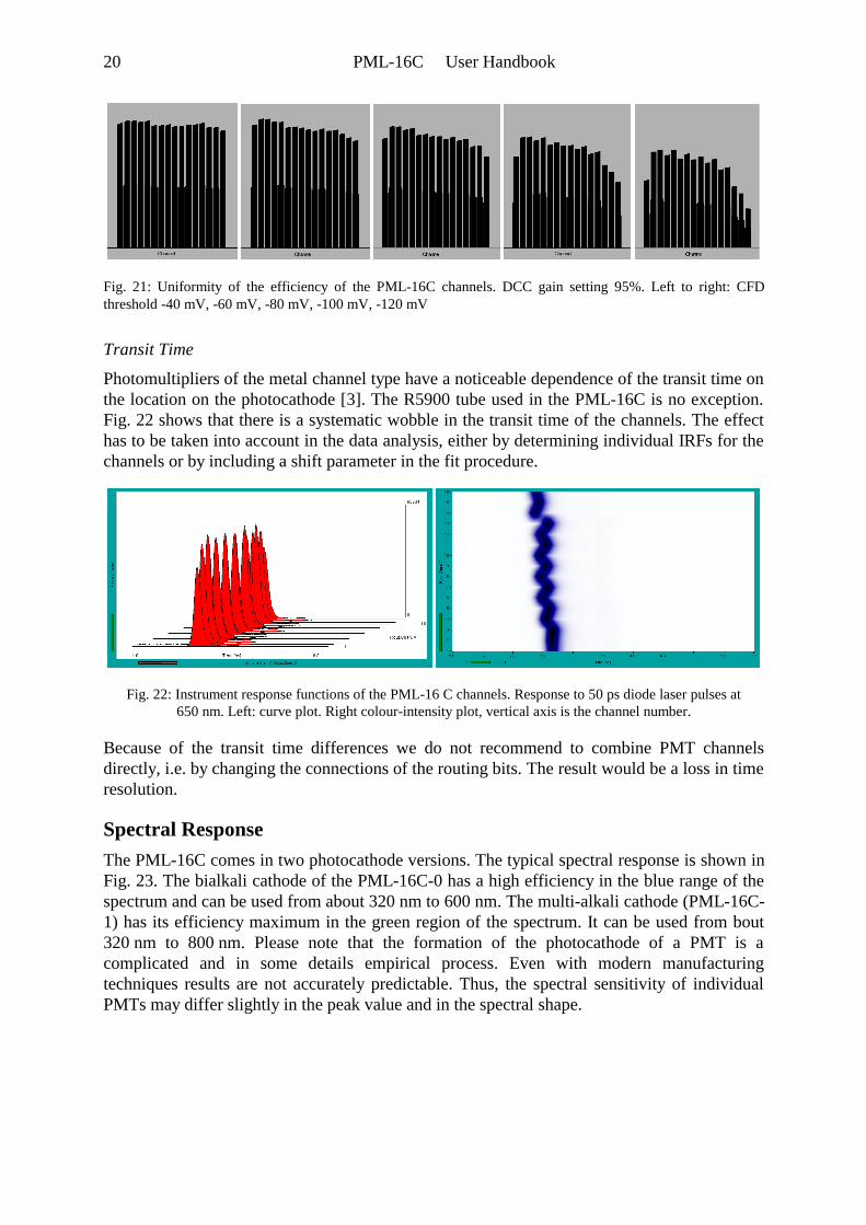
A practical example is given in Fig. 21. The channels of a PML-16C were evenly illuminatedwith continuous light. The DCC gain was set to 95%, corresponding to a PMT operatingvoltage of 950 V. From left to right, the CFD threshold was increased from -40 mV to-120 mV. It can clearly be seen that with increasing CFD threshold there is not only a decreasein efficiency but also a degradation in the channel uniformity.


Fig. 21: Uniformity of the efficiency of the PML-16C channels. DCC gain setting 95%. Left to right: CFDthreshold -40 mV, -60 mV, -80 mV, -100 mV, -120 mV

Transit Time

Photomultipliers of the metal channel type have a noticeable dependence of the transit time onthe location on the photocathode [3]. The R5900 tube used in the PML-16C is no exception.Fig. 22 shows that there is a systematic wobble in the transit time of the channels. The effecthas to be taken into account in the data analysis, either by determining individual IRFs for thechannels or by including a shift parameter in the fit procedure.

Fig. 22: Instrument response functions of the PML-16 C channels. Response to 50 ps diode laser pulses at650 nm. Left: curve plot. Right colour-intensity plot, vertical axis is the channel number.

Because of the transit time differences we do not recommend to combine PMT channelsdirectly, i.e. by changing the connections of the routing bits. The result would be a loss in timeresolution.

Spectral Response

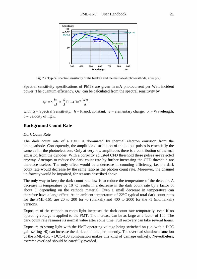
The PML-16C comes in two photocathode versions. The typical spectral response is shown inFig. 23. The bialkali cathode of the PML-16C-0 has a high efficiency in the blue range of thespectrum and can be used from about 320 nm to 600 nm. The multi-alkali cathode (PML-16C-1) has its efficiency maximum in the green region of the spectrum. It can be used from bout320 nm to 800 nm. Please note that the formation of the photocathode of a PMT is acomplicated and in some details empirical process. Even with modern manufacturingtechniques results are not accurately predictable. Thus, the spectral sensitivity of individualPMTs may differ slightly in the peak value and in the spectral shape.


300 400 500 600 700 800 900nm

10

100

1

mA/W

Wavelength

Sensitivity

bialkalimultialkali

QE=0.2QE=0.1

Fig. 23: Typical spectral sensitivity of the bialkali and the multialkali photocathode, after [22].

Spectral sensitivity specifications of PMTs are given in mA photocurrent per Watt incidentpower. The quantum efficiency, QE, can be calculated from the spectral sensitivity by

A

Wm1024.1 6−⋅⋅==

λλS

e

hcSQE

with S = Spectral Sensitivity, h = Planck constant, e = elementary charge, λ = Wavelength,c = velocity of light.

Background Count Rate

Dark Count Rate

The dark count rate of a PMT is dominated by thermal electron emission from thephotocathode. Consequently, the amplitude distribution of the output pulses is essentially thesame as for the photoelectrons. Only at very low amplitudes there is a contribution of thermalemission from the dynodes. With a correctly adjusted CFD threshold these pulses are rejectedanyway. Attempts to reduce the dark count rate by further increasing the CFD threshold aretherefore useless. The only effect would be a decrease in counting efficiency, i.e. the darkcount rate would decrease by the same ratio as the photon count rate. Moreover, the channeluniformity would be impaired, for reasons described above.

The only way to keep the dark count rate low is to reduce the temperature of the detector. Adecrease in temperature by 10 °C results in a decrease in the dark count rate by a factor ofabout 5, depending on the cathode material. Even a small decrease in temperature cantherefore have a large effect. At an ambient temperature of 22°C typical total dark count ratesfor the PML-16C are 20 to 200 for -0 (bialkali) and 400 to 2000 for the -1 (multialkali)versions.

Exposure of the cathode to room light increases the dark count rate temporarily, even if nooperating voltage is applied to the PMT. The increase can be as large as a factor of 100. Thedark count rate resumes its normal value after some time. Full recovery can take several hours.

Exposure to strong light with the PMT operating voltage being switched on (i.e. with a DCCgain setting >0) can increase the dark count rate permanently. The overload shutdown functionof the PML-16C - DCC-100 combination makes this kind of damage unlikely. Nevertheless,extreme overload should be carefully avoided.


Afterpulsing

The dark count rate is often considered the only source of signal background. Signalbackground can, however, also be caused by afterpulsing. All photon-counting detectors (alsosingle-photon avalanche photodiodes) have an increased probability of producing backgroundpulses within a few microseconds following the detection of a photon. These afterpulses aredetectable in almost any conventional PMT. It is believed that they are caused by ionfeedback, or, by a smaller amount, by luminescence of the dynode material and the glass ofthe tube.

Afterpulsing becomes noticeable especially in high-repetition rate TCSPC applications, inparticular with Ti:Sapphire lasers or diode lasers. At high repetition rate, the afterpulses frommany signal periods pile up and can cause a considerable signal-dependent background. Thetotal afterpulsing rate can easily exceed the dark count rate of the detector by a factor of 100[2, 3].

The R5900-L16 tubes used in the PML-16C have a relatively low afterpulsing probability andthus deliver an excellent dynamic range in high-repetition rate applications. Fig. 24, upperrow, shows a recording of a fluorescence signal, taken with a PML-16C-0 in PML-SPECmulti-spectral detection assembly (see paragraph below).

-

Fig. 24: Background by afterpulsing. Left: Fluorescence signal. Right: Dark counts. Upper row: All 16wavelength channels. Lower row: Channel with maximum fluorescence intensity. Laser pulse repetition rate

20 MHz, acquisition time 100 seconds.

The acquisition time was 100 seconds. The excitation pulse rate was 20 MHz, the acquisitiontime 100 seconds. The complete multi-spectral decay data are shown left, the channel of


highest intensity right. The useful dynamic range (peak to background) is more than 4 ordersof magnitude, about as good as for an MCP PMT [3].

A dark recording taken with the same acquisition time and pulse repetition rate as thefluorescence recording is shown in the lower row of Fig. 24. It is obvious that the dark countlevel is lower than the background of the fluorescence recording. The average backgroundlevels are 1.8 and 0.015, respectively. Thus, also for the PML-16C the dynamic range at highpulse repetition rate is limited by afterpulsing, not by the dark count rate.

The straightforward way to reduce the afterpulsing background is to reduce the signalrepetition rate. However, to keep pile-up effects low the count rate must be reduced [2, 3]. Thetradeoff is therefore an increased acquisition time.


PML-SPEC AssemblyThe PML-SPEC multi-wavelength detection assembly is a combination of the PML-16C and asmall grating polychromator (or spectrograph). The assembly is shown in Fig. 25.

Fig. 25: PML-SPEC multi-wavelength detection assembly, shown with a fibre bundle at the input

The PML-SPEC is available with three different gratings, see table below. The gratingdetermines the dispersion and thus the wavelength interval recorded via the 16 channels of thePML-16C. The start wavelength of the interval is selectable by a micrometer screw at thepolychromator.

Grating Primary wavelength region Width of recorded wavelength Blaze WavelengthPart No. adjustable by set screw interval, channel 1 to 1677417 340-820 nm 300 nm 500 nm77414 (standard) 340-820 nm 200 nm 400 nm77411 340-820 nm 100 nm 350 nm

The blaze wavelength is the wavelength the grating is optimised for. The amount of lightdiffracted into the first diffraction order is at maximum at this wavelength. However, even at awavelength close to the blaze wavelength a grating disperses some light into higher diffractionorders. The light of the unused orders can cause substantial straylight problems. Influorescence applications the PML-SPEC should therefore be used with an additional filterthat blocks the excitation wavelength.

There are several ways to deliver the light into the input slit plane of the polychromator. Free-beam coupling is often used in the traditional fluorescence lifetime setups. In these cases alens transfers the luminescent spot in the sample into the input slit of the polychromator. Theparameters of this lens have a considerable influence on the optical efficiency.

The polychromator accepts light within a focal ratio (or ‘f number’) of about 1:3.5. To obtainmaximum light throughput, the f number of the input light cone must match the f number ofthe monochromator. Moreover, the image in the input plane must not be larger than the slit.Building an appropriate relay lens system is no problem if the light comes from a point source.For larger sources the throughput is limited by the slit size and the f number of themonochromator; see Fig. 26.


Sourceof

Emission

Lens Polychromator, f / n

f / n

Sourceof

Emission

Lens Polychromator, f / n

f / n

Image onmonochromatorslit

Image on

slitinput

Sourceof

Emission

Lens

Polychromator, f / n

f / n

Image oninputslit

> f / n

a) f number matchedslit fully illuminated

b) f number too highslit fully illuminated, but c) f number matched, but

slit over-illuminated

unused

used

Fig. 26: Limitations of the light throughput of a polychromator. Once the slit is fully illuminated and thef numbers are equal, neither (a) a larger lens nor (b) a lens with a higher NA at the source side will increase the

throughput.

Once the input light cone matches the f number of the polychromator (a), neither (b) a largerlens nor (c) a lens with a higher NA at the source side will increase the amount of transmittedlight. Case (b) leads to an input cone of a larger f number than accepted by the polychromator.Case (c) results in an image larger than the polychromator slit. In both cases the additionallight transferred by the lens is not transmitted through the polychromator.

Please note that relatively wide input slits can be used for the PML-SPEC. The centre distanceof the PML-16C channels is 1 mm. Reducing the slit width far below this value does not yieldany gain in resolution. Thus, the optimum slit width is in the range of 05. to 1 mm.

Another way to increase the throughput is to reduce the size of the excited spot in the sampleor to match the shape of the source spot to the monochromator slit. In cuvette fluorescencesystems with a horizontal excitation beam a large improvement can be made by turning thepolychromator 90°, so that the slit is horizontal and matches the orientation of the excitedsample volume.

Another way to couple light into the PML-SPEC is via an optical fibre. For fibre-coupledsystems the input slit of the polychromator is replaced with a fibre adapter, with the end of thefibre placed in the slit plane. The coupling efficiency from the fibre into the polychromator isthen almost ideal. However, coupling the light into the fibre has to cope with the same basicoptical problems as coupling the light directly into the polychromator slit. Fibre diameters upto 1 mm can be used without much compromise in wavelength resolution. Fibre-coupledsystems are used to connect the PML-SPEC to confocal scan heads of laser scanningmicroscopes [8], see Fig. 27. Fibre-coupling has also been used for diffuse optical tomography(DOT). A super-continuum was generated by sending the pulses of a Ti:Sapphire laser thougha photonic crystal fibre. After propagating of the continuum pulses through the tissue the lightwas collected via a multi-mode fibre, and the time-of-flight distributions were recorded in 16wavelength intervals [1].

An elegant way to increase the throughput of a fibre-coupled system is to use several fibres ora fibre bundle (see Fig. 28 and Fig. 30). The fibres are arranged along the slit of thepolychromator. The fibre system is thus used to collect light from an increased area andtransform the cross-section of this area into the cross section of the slit.


MW-FLIM Multi-Wavelength FLIM Detection SystemsThe PML-SPEC assembly is used for bh’s modular fluorescence lifetime imaging (FLIM)systems for laser scanning microscopy [3, 5]. Laser scanning microscopes scan the sample bya focused laser beam and detect the fluorescence from the excited spot by a single-pointdetector. Confocal microscopes use a pinhole in the detection light path to suppress light fromoutside the focal plane [27]. Two-photon microscopes excite the fluorescence by afemtosecond laser of high repetition rate. Two photons of the input light are used to generateone fluorescence photon [18, 19]. Two-photon excitation is nonlinear and thus yieldsnoticiable excitation only in the focus of the microscope objective lens. Therefore excitationoutside the focal plane is avoided altogether.

One-Photon Excitation with Confocal Detection

The general setup of a confocal multi-wavelength FLIM system is shown in Fig. 27. A bhBDL-405-SM diode laser [14] delivers picosecond pulses into one of the laser input fibres ofthe scanning microscope. In order to obtain diffraction-limited focusing the laser scanningmicroscopes use single-mode fibres for the laser input. Therefore the -SM (single-mode)version of the BDL-405 must be used. The power of the laser is controlled via the DCC-100card.

The fluorescence light from the scanned spot of the sample is fed into the PML-SPEC via amulti-mode fibre output from the scan head. Fibre outputs are available for almost all modernlaser scanning microscopes. Diode-laser based confocal MW-FLIM systems are available forthe Zeiss LSM 510, the Olympus FV1000, and the Leica SP2 or SP5.

PolychromatorTCSPC Module

Microscope

Scanhead

Grating

Input fibre

single mode

Output fibremulti mode

BDL-405-SM picosecond diode laser

PML-16C

DCC-100Power control

Fig. 27: Multi-wavelength FLIM system, one-photon excitation by picosecond diode laser, confocal detection

The TCSPC module is operated in the ‘Scan Sync In’ mode. In this mode the recording in theTCSPC module is synchronised with the scanning by pixel clock, line clock, and frame clockpulses from the microscope. The TCSPC module builds up a photon distribution over the timein the laser pulse period, the coordinates of the scan, and the wavelength [2, 3, 5]. Because ofthe large amount of data to be kept in the TCSPC memory an SPC-830 module should beused.

Two-photon Excitation with Descanned Detection

With a femtosecond Ti:Sapphire laser the sample can be excited by two-photon absorption[18, 19]. In a microscope, two-photon excitation works with high efficiency because theenergy density in the focus of a high-NA objective lens is high. Noticeable excitation is


obtained only in the focus. Therefore two-photon excitation inherently delivers depthresolution. Confocal detection through a pinhole is not required. Nevertheless, thefluorescence light can be fed back through the scanner and the pinhole. The optical setup ofthe detection light path is then identical with the one used for one-photon excitation. Systemwith two-photon excitation and detection via the confocal beam path have been used forFRET experiments [8, 17] and for PDT experiments on the cell level [28].

Two-photon Excitation with Non-Descanned Detection

Because two-photon excitation does not generate fluorescence outside the focus no light fromoutside the focal plane needs to be rejected. The fluorescence light can therefore be diverteddirectly behind the microscope objective by a dichroic mirror. This setup is called ‘non-descanned’ or ‘direct’ detection in contrast to the ‘confocal’ or ‘descanned detection’ used forone-photon excitation.

Two-photon excitation in conjunction with non-descanned detection can be used to imagetissue layers several 100 µm deep [18, 21]. Since the scattering and the absorption coefficientsat the wavelength of the two-photon excitation are small the laser beam penetrates throughrelatively thick tissue. Even if there is some loss on the way through the tissue it can becompensated by increasing the laser power. Of course, the fluorescence photons are scatteredon their way out of the tissue and therefore emerge from a relatively large area of the samplesurface. Moreover, the surface is not in the focus of the objective lens. The fluorescence lighttherefore leaves the full back aperture of the microscope lens in a cone of relatively largeangle. A multi-wavelength system for non-descanned detection systems has to transfer thislight into the polychromator.

The first multi-spectral FLIM system for two-photon microscopes with non-descanneddetection was described in [16]. An image of the aperture of the microscope objective lenswas projected on the input of a 1-mm multi-mode fibre. The fibre delivered the fluorescencelight to a polychromator. The spectrum was recorded by a bh PML-16 detector, and the 16wavelength channels were recorded simultaneously by a bh SPC-830 module. The problem ofthe optical setup used was that a strong demagnification into the fibre has to be used. Thisresults in a high numerical aperture of the light cone at the input of the fibre. However, amulti-mode fibre used near its maximum NA develops strong pulse dispersion [24]. The IRFof the system is therefore noticeably broader than the IRF of the PML-16. Moreover, the shortfocal length required for the projection into the fibre results in a small diameter of the lens.The system therefore loses efficiency for deep layers of highly scattering samples.

The bh NDD MW-FLIM systems use a fibre bundle to transform the circular cross section ofthe microscope lens aperture into the linear cross section of the polychromator slit. Theprinciple is shown in Fig. 28.


Polychromator

Crosssectionof bundle

750 nm to 900 nm

Microscope

Scan Ti:Sa Laser

Shutter

Filter

head

Fibre bundle

Grating

Lens

TCSPC ModulePML-16C

DCC-100

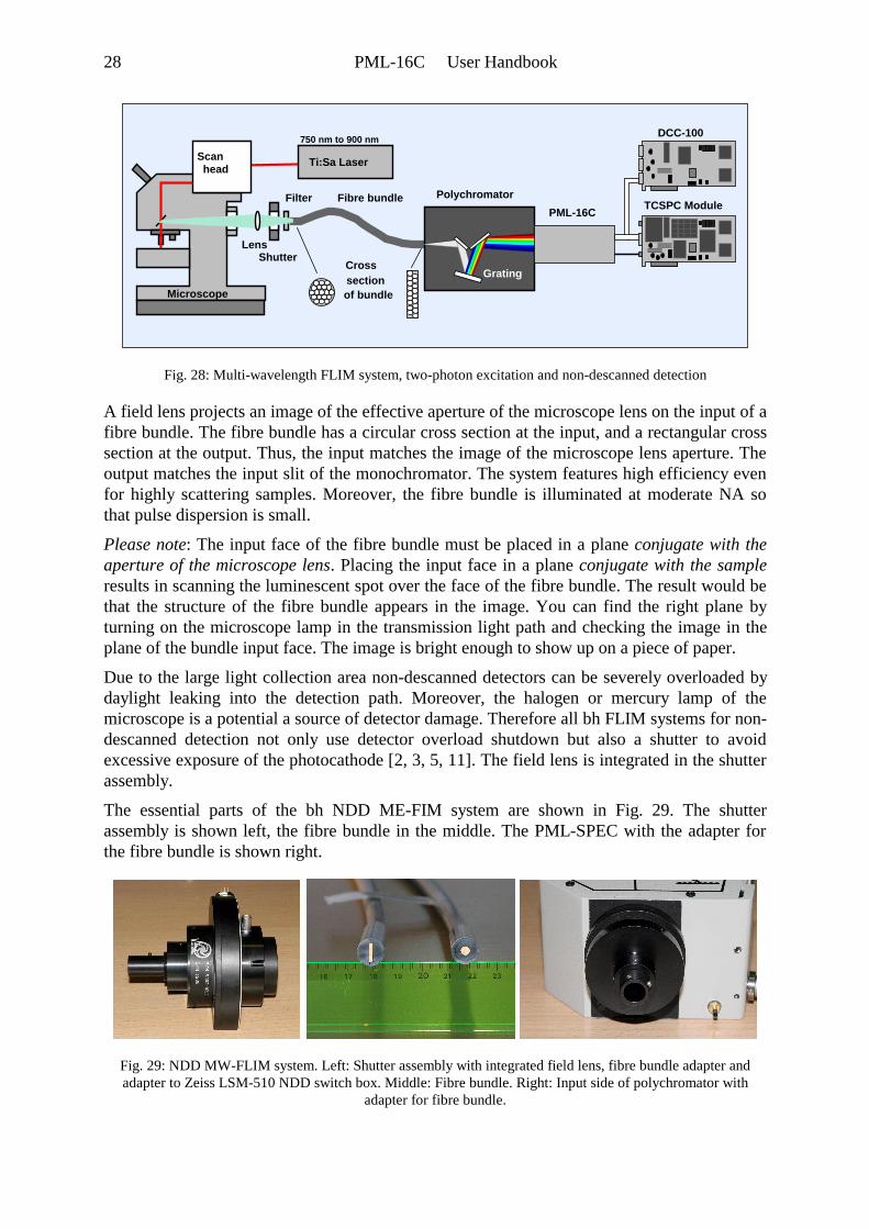
Fig. 28: Multi-wavelength FLIM system, two-photon excitation and non-descanned detection

A field lens projects an image of the effective aperture of the microscope lens on the input of afibre bundle. The fibre bundle has a circular cross section at the input, and a rectangular crosssection at the output. Thus, the input matches the image of the microscope lens aperture. Theoutput matches the input slit of the monochromator. The system features high efficiency evenfor highly scattering samples. Moreover, the fibre bundle is illuminated at moderate NA sothat pulse dispersion is small.

Please note: The input face of the fibre bundle must be placed in a plane conjugate with theaperture of the microscope lens. Placing the input face in a plane conjugate with the sampleresults in scanning the luminescent spot over the face of the fibre bundle. The result would bethat the structure of the fibre bundle appears in the image. You can find the right plane byturning on the microscope lamp in the transmission light path and checking the image in theplane of the bundle input face. The image is bright enough to show up on a piece of paper.

Due to the large light collection area non-descanned detectors can be severely overloaded bydaylight leaking into the detection path. Moreover, the halogen or mercury lamp of themicroscope is a potential a source of detector damage. Therefore all bh FLIM systems for non-descanned detection not only use detector overload shutdown but also a shutter to avoidexcessive exposure of the photocathode [2, 3, 5, 11]. The field lens is integrated in the shutterassembly.

The essential parts of the bh NDD ME-FIM system are shown in Fig. 29. The shutterassembly is shown left, the fibre bundle in the middle. The PML-SPEC with the adapter forthe fibre bundle is shown right.

Fig. 29: NDD MW-FLIM system. Left: Shutter assembly with integrated field lens, fibre bundle adapter andadapter to Zeiss LSM-510 NDD switch box. Middle: Fibre bundle. Right: Input side of polychromator with

adapter for fibre bundle.


The NDD MW-FLIM systems are available for the Zeiss LSM 510 NLO microscopes and forLeica SP2 and SP5 MP systems. The shutter assembly of the MW-FLIM connects to the NDDswitch box of the LSM 510 and to the RLD port of the SP2 or SP5. The assemblies can,however, easily be adapted to non-descanned ports of other microscopes.


Applications

Single-point tissue spectroscopy

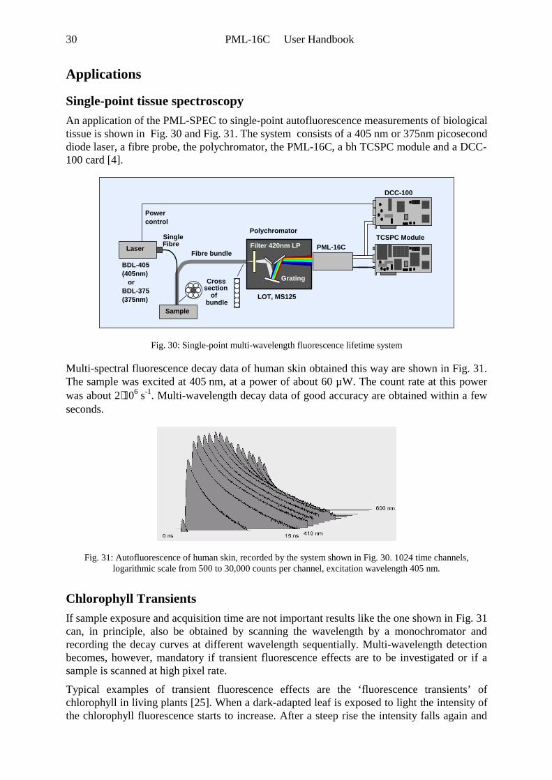
An application of the PML-SPEC to single-point autofluorescence measurements of biologicaltissue is shown in Fig. 30 and Fig. 31. The system consists of a 405 nm or 375nm picoseconddiode laser, a fibre probe, the polychromator, the PML-16C, a bh TCSPC module and a DCC-100 card [4].

Polychromator

Laser

SingleFibre

Fibre bundle

Crosssection

of

Sample

(405nm)BDL-405

PML-16C

LOT, MS125bundle

Grating

Filter 420nm LPTCSPC Module

DCC-100

orBDL-375(375nm)

Powercontrol

Fig. 30: Single-point multi-wavelength fluorescence lifetime system

Multi-spectral fluorescence decay data of human skin obtained this way are shown in Fig. 31.The sample was excited at 405 nm, at a power of about 60 µW. The count rate at this powerwas about 2⋅106 s-1. Multi-wavelength decay data of good accuracy are obtained within a fewseconds.

Fig. 31: Autofluorescence of human skin, recorded by the system shown in Fig. 30. 1024 time channels,logarithmic scale from 500 to 30,000 counts per channel, excitation wavelength 405 nm.

Chlorophyll Transients

If sample exposure and acquisition time are not important results like the one shown in Fig. 31can, in principle, also be obtained by scanning the wavelength by a monochromator andrecording the decay curves at different wavelength sequentially. Multi-wavelength detectionbecomes, however, mandatory if transient fluorescence effects are to be investigated or if asample is scanned at high pixel rate.

Typical examples of transient fluorescence effects are the ‘fluorescence transients’ ofchlorophyll in living plants [25]. When a dark-adapted leaf is exposed to light the intensity ofthe chlorophyll fluorescence starts to increase. After a steep rise the intensity falls again and


finally reaches a steady-state level. The rise time is of the order of a few milliseconds to asecond, the fall time can be from several seconds to minutes. The initial rise of thefluorescence intensity is attributed to the progressive closing of reaction centres in thephotosynthesis pathway. Therefore the quenching of the fluorescence by the photosynthesisdecreases with the time of illumination, with a corresponding increase of the fluorescenceintensity. The fluorescence quenching by the photosynthesis pathway is termed‘photochemical quenching’. The slow decrease of the fluorescence intensity at later times istermed ‘non-photochemical quenching’.

Results of a non-photochemical quenching measurement are shown in Fig. 32. Thefluorescence in a leaf was excited by a bh BDL-405 (405 nm) picosecond diode laser.Simultaneously with the switch-on of the laser a recording sequence was started in the TCSPCmodule. 30 recordings were taken in intervals of 2 seconds; Fig. 32 shows four selected stepsof this sequence. The decrease of the fluorescence lifetime with the time of exposure is clearlyvisible.

Fig. 32: Non-photochemical quenching of chlorophyll in a leaf, excited at 405 nm. Recorded wavelength rangefrom 620 to 820 nm, time axis 0 to 8 ns, logarithmic display, normalised on peak intensity. Left to right: 0 s, 20 s,40 s, and 60 s after start of exposure.

Fig. 33 shows fluorescence decay curves at selected wavelengths versus the time of exposure,extracted from the same measurement data set as Fig. 32. The sequence starts at the back andextends over 60 seconds. Also here, the decrease of the fluorescence lifetime with the time ofexposure is clearly visible.

Fig. 33: Non-photochemical quenching of chlorophyll in a leaf, excited at 405 nm. Fluorescence decay curves indifferent wavelength channels versus time of exposure. 2 s per curve, sequence starts from the back. Extractedfrom same measurement data as Fig. 32.

The non-photochemical transients shown above occur on a time scale of several 10 seconds.Good results are therefore obtained by recording a single sequence of decay curves at anacquisition time of a few seconds per curve.

The photochemical quenching transients are much faster. Recording these transients requires aresolution of less than 100 µs per step of the sequence. Of course, the number of photonsdetected in a time this short is too small to build up a resonable decay curve. Photochemicalquenching transients must therefore be recorded by triggered sequential recording [2, 3]. Theprinciple is shown in Fig. 34. The excition laser is periodically switched on an off. Each ‘on’phase initiates a photochemical quenching transient in the leaf; each ‘off’ phase lets the leaf


rcover. Within each ‘on’ phase a fast sequence of decay curves is recorded in the TCSPCmodule. The measurement is continued for a large number of such on-off cycles, and theresults are accumulated.

Laseron

off

on

Experiment trigger

to SPC module

Recording Recording

Leaf recovers

sequence sequence

2.5ms 90ms 2.5ms

Fig. 34: Triggered sequential recording of photochemical quenching transients. The laser is cycled on and off.Each ‘on’ phase starts a photochemical quenching transient in the leaf. A sequence of waveform recordings istaken within each ‘on’ phase. A large number of such on/off cycles is accumulated to obtain enough photons withthe individual steps of the accumulated sequence.

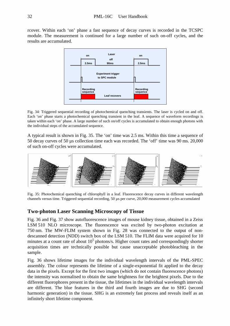
A typical result is shown in Fig. 35. The ‘on’ time was 2.5 ms. Within this time a sequence of50 decay curves of 50 µs collection time each was recorded. The ‘off’ time was 90 ms. 20,000of such on-off cycles were accumulated.

Fig. 35: Photochemical quenching of chlorophyll in a leaf. Fluorescence decay curves in different wavelengthchannels versus time. Triggered sequential recording, 50 µs per curve, 20,000 measurement cycles accumulated

Two-photon Laser Scanning Microscopy of Tissue

Fig. 36 and Fig. 37 show autofluorescence images of mouse kidney tissue, obtained in a ZeissLSM 510 NLO microscope. The fluorescence was excited by two-photon excitation at750 nm. The MW-FLIM system shown in Fig. 28 was connected to the output of non-descanned detection (NDD) switch box of the LSM 510. The FLIM data were acquired for 10minutes at a count rate of about 105 photons/s. Higher count rates and correspondingly shorteracquisition times are technically possible but cause unacceptable photobleaching in thesample.

Fig. 36 shows lifetime images for the individual wavelength intervals of the PML-SPECassembly. The colour represents the lifetime of a single-exponential fit applied to the decaydata in the pixels. Except for the first two images (which do not contain fluorescence photons)the intensity was normalised to obtain the same brightness for the brightest pixels. Due to thedifferent fluorophores present in the tissue, the lifetimes in the individual wavelength intervalsare different. The blue features in the third and fourth images are due to SHG (secondharmonic generation) in the tissue. SHG is an extremely fast process and reveals itself as aninfinitely short lifetime component.


Fig. 36: Autofluorescence FLIM images of living mouse kidney tissue.

An increased signal-to-noise ratio is obtained by combining the decay data of severalwavelength intervals, see Fig. 37. The upper row shows single-exponential lifetime images inwavelength intervals of 350 to 380 nm, 380 to 430 nm, 430 to 480 nm, and 480 to 530 nm.

The second row, left, shows the fluorescence decay curve at the cursor position of the 430 to480 nm image. Even at first glance it can be seen that the decay is not single-exponential. Agood fit can be obtained by a double-exponential fit. The lifetime images in the second rowshow the fast decay component, the slow decay component, and the amplitude ratio of both.The fluorescence in the 430 to 480 nm interval is dominated by NADH. The lifetime ofNADH is known to depend on the binding to proteins [23]. The images can therefore expectedto represent different binding states of NADH.

Fig. 37: Upper row: Single-exponential lifetime images in selected wavelength intervals. Lower row, left to right:Fluorescence decay curve at cursor position of 430 to 480 nm image with double exponential fit (red), lifetimeimage of the fast decay component, lifetime image of the slow decay component, image of the amplitudes of thelifetime components.


TroubleshootingIf the PML / SPC system does not work as expected please check the following details:

All count rates are present, but no curves or not all curves are displayed

Check that 'Points X' is set to ‘16’ and that you have set a reasonable ‘Delay’ in the pagecontrol section of the System Parameters. In the ‘Single’ or ‘Oscilloscope’ mode, check the2D Trace parameters. Make sure that the correct ‘curves’ are displayed, and that the ‘Page’ isthe same as ‘Measured Page’ in the main panel. Please see Fig. 8.

No CFD count rate

Check the DCC settings. The +12V, +5V, and -5V buttons must be enabled, and the outputsmust be enabled (see Fig. 12). Please note that, for safety reasons, the DCC-100 starts with alloutputs disabled. Make sure that a reasonable gain is set. Single photon detection requires again above 80%, correct operation typically 90 to 95%. Make sure that the 15 pin powersupply cable is connected to the upper or lower connector of the DCC-100 and that youcontrol the DCC parameters of the right connector. Make sure that the 50-Ω SMA cable isconnected from the PML output to the CFD input.

Large differences in channel efficiency, large crosstalk between channels

Increase DCC gain or decrease CFD threshold. Make sure that ‘Delay’ in the page controlsection of the System Parameters is set correctly. Check your system for electrical noise.Disconnect a network cable possibly connected to the computer.

CFD rate present, but no ADC rate

Make sure that the SYNC signal is present at the Sync input of the SPC card. The SYNC rateshould correspond to the repetition rate of the light source used. Make sure that the 15 pinrouting cable is connected to the routing connector of the SPC card. Some SPC cards havetwo connectors; the right connector is the one closer to the computer motherboard.

CFD rate present, but ADC rate very low. Only random photons detected.

The signal is outside the recorded time range. This happens especially for low-repetition ratesignals. Usually the delay in the SYNC channels is too small. It may then happen that a timeinterval shortly before the laser pulse is recorded. See [3]; the SYNC pulse should arrive some10 ns after the photon pulses. Make sure that the light arrives at the detector. If you haveoptical fibres feeding the light into a PML-SPEC assembly, check that the fibres are notbroken and correctly connected. Make sure that the fibre is really an optical fibre and not anelectrical SMA cable.

Another detector connected to the SPC module refuses to work

Disconnect the routing cable from the SPC module. When the PML is inactive it delivers a‘disable count’ signal.

Poor time resolution, poor shape of IRF

Check your system for electrical noise. Disconnect a network cable possibly connected to thecomputer. Check for optical effects, such as photon migration in a scattering solution, andoptical reflections.

Signals are detected even for DCC gain = 0

Check the CFD threshold. It should be between -50 mV and -100 mV. Check your system forelectrical noise. Disconnect a network cable that is possibly connected to the computer.


Assistance through bhSoftware updates, new handbook versions and application notes are available from the bh website, www.becker-hickl.de. Furthermore, we are pleased to support you in all problemsconcerning the measurement of fast electrical or optical signals. This includes discussions ofnew applications, the installation of the SPC modules, their application to your measurementproblem, the technical environment and physical problems related to time-resolvedspectroscopy. Simply call us or send us an email.

Should there be a problem with your PML or SPC module, please contact us. To fix theproblem we ask you to send us a data file (.sdt) of the questionable measurement or, if ameasurement is not possible, a setup file (.set) with your system settings. Furthermore, pleaseadd as much as possible of the following information:

Description of the ProblemSPC and PML Module, Type and Serial NumberSoftware VersionDetector type, PMT Cathode typeDCC-100 settingsLaser System: Type, Repetition Rate, Wavelength, PowerSYNC Signal Generation: Photodiode, Amplitude, Rise TimeOptical System: Basic Setup, Sample, MonochromatorSystem Connections: Cable Lengths, Ground Connections. Add a drawing if necessary.Environment: Possible Noise SourcesYour personal data: E-mail, Telephone Number, Postal Address

The fastest way is to send us an email with the data file(s) attached. We will check yoursystem settings and – if necessary – reproduce your problem in our lab. We will send you ananswer within one or two days.

Becker & Hickl GmbHNahmitzer Damm 3012277 BerlinTel. +49 / 30 / 787 56 32FAX +49 / 30 / 787 57 34http://www.becker-hickl.deemail: [email protected]


Specification

ElectricalNumber of Channels 16Arrangement linear (1 by 16)Active Area (each channel) 0.8 × 16 mmChannel Pitch 1 mmSpectral response 300 to 650 nm (bialkali)

185 to 650 nm (bialkali, UV window)300 to 820 nm (multialkali)

Dark count rate (total, 22°C, typical values) Bialkali 100 counts per secondMultialkali 1000 counts per second

Timing Output Polarity negativeAverage Timing Pulse Amplitude 50 to 100 mV at -900VTime Resolution (FWHM of IRF) 150 ps (typical value, for individual channels)Time Skew between Channels < 100 psTiming Output Connector SMA, 50ΩMisrouted Photons (100 kHz Count Rate) < 0.1 %Suppressed Photons (100 kHz Count Rate) < 1 %Routing Signal 4 ‘Channel’ bits + ‘Disable Count’ bit, TTL/CMOSOptimum 'Latch Delay' in SPC module 0 ns (SPC-630, 730, 830)

20 ns (SPC-140)Connector for routing and power supply 15 pin Sub-D / HD (3 rows of pins)Power Supply +5V, -5V, +12V, from DCC-100 cardGain control signal 0 to 1V, from DCC-100 cardOverload shutdown at >2µA channel current, via DCC-100 cardDimensions 50 mm × 50 mm × 168 mm

15 Pin Sub-D HD connector Pin assignment

1 +5 V2 Routing, /R0 (TTL)3 Routing, /R1 (TTL)4 Routing, /R2 (TTL)5 GND6 -5 V7 Routing, /R3 (TTL)8 do not connect9 do not connect10 +12 V11 do not connect12 /Overload (TTL, open collector)13 Gain Control, 0 to 1 V14 /Disable Count (TTL)15 GND


Mechanical

R5900 PMT

27

34

40

27 34 40 50

50

M 2.5

7.5

6

2.5

Front face to PMT window

16x16

activearea

Fig. 38: Front end, outline in millimeters

50

168

Fig. 39: Side View, outline in millimeters

16

16

Distance 1mm

Fig. 40: Active area of photocathode, outline in millimeters


References

1. A. Bassi, J. Swartling, C. D’Andrea, A. Pifferi, A. Torricelli, R. Cubeddu, Time-resolvedspectrophotometer for turbid media based on supercontinuum generation in a photonic crystal fibre, Opt.Lett. 29, 2405-2407 (2004)

2. W. Becker, Advanced time-correlated single-photon counting techniques. Springer, Berlin, Heidelberg,New York, 2005

3. W. Becker, The bh TCSPC Handbook, Becker & Hickl GmbH, available on www.becker-hickl.com (2005)4. W. Becker, A. Bergmann, C. Biskup, D. Schweitzer, M. Hammer, Time- and Wavelength-Resolved

Autofluorescence Detection by Multi-Dimensional TCSPC, Proc. SPIE 5862, 174-181 (2005)5. W. Becker, A. Bergmann, M.A. Hink, K. König, K. Benndorf, C. Biskup, Fluorescence lifetime imaging by

time-correlated single photon counting, Micr. Res. Techn. 63, 58-66 (2004)6. W. Becker, A. Bergmann, G. Biscotti, K. Koenig, I. Riemann, L. Kelbauskas, C. Biskup, High-speed FLIM

data acquisition by time-correlated single photon counting, Proc. SPIE 5323, 27-35 (2004)7. W. Becker, A. Bergmann, Timing Stability of TCSPC Experiments, Becker & Hickl GmbH (2004),

available on www.becker-hickl.com8. W. Becker, A. Bergmann, C. Biskup, T. Zimmer, N. Klöcker, K. Benndorf, Multi-wavelength TCSPC

lifetime imaging, Proc. SPIE 4620 79-84 (2002)9. W. Becker, A. Bergmann, H. Wabnitz, D. Grosenick, A. Liebert, High count rate multichannel TCSPC for

optical tomography, Proc. SPIE 4431, 249-245 (2001)10. W. Becker, Verfahren und Vorrichtung zur Messung von Lichtsignalen mit zeitlicher und räumlicher

Auflösung, Patent DE 43 39 787 (1993)11. W. Becker, A. Bergmann, Detector assemblies for picosecond microscopy, Becker & Hickl GmbH,

www.becker-hickl.com12. Becker & Hickl GmbH, DCC-100 detector control module, manual, www.becker-hickl.com13. Becker & Hickl GmbH, 16 channel detector head for time-correlated single photon counting, manual,

www.becker-hickl.com14. Becker & Hickl GmbH, BDL-375, BDL-405, BDL-475 Ultraviolet and Blue Picosecond Diode Laser

Modules, www.becker-hickl.com15. A. Bergmann, SPCImage Data Analysis Software for Fluorescence Lifetime Imaging Microscopy,

Becker & Hickl GmbH, available on www.becker-hickl.com16. D.K. Bird, K.W. Eliceiri, C-H. Fan, J.G. White, Simultaneous two-photon spectral and lifetime

fluorescence microscopy, Appl. Opt. 43, 5173-5182 (2004)17. C. Biskup, L. Kelbauskas, Th. Zimmer, S. Dietrich, K. Benndorf, W. Becker, A. Bergmann, N. Klöcker,

Spectrally resolved fluorescence lifetime and FRET measurements, Proc. SPIE 5700, 188-196 (2005)18. W. Denk, J.H. Strickler, W.W.W. Webb, Two-photon laser scanning fluorescence microscopy, Science

248, 73-76 (1990)19. M. Göppert-Mayer, Über Elementarakte mit zwei Quantensprüngen, Ann. Phys. 9, 273-294 (1931)20. Hamamatsu Photonics K.K., R5900U-16 series Multianode photomultiplier tube (2001)21. K. König, Multiphoton microscopy in life sciences, J. Microsc. 200, 83-104 (2000)22. H. Kume (ed.), Photomultiplier Tube, Hamamatsu Photonics K.K. (1994)23. J.R. Lakowicz, Principles of Fluorescence Spectroscopy, 2nd edn., Plenum Press, New York (1999)24. A. Liebert, H. Wabnitz, D. Grosenick, R. Macdonald, Fiber dispersion in time domain measurements

compromising the accuracy of determination of optical properties of strongly scattering media, J. Biomed.Opt. 8, 512-516 (2003)

25. K. Maxwell, G.N. Johnson, Chlorophyll fluorescence - a practical guide, Journal of Experimental Botany51, 659-668 (2000)

26. D.V. O’Connor, D. Phillips, Time-correlated single photon counting, Academic Press, London (1984)27. J. Pawley (ed.), Handbook of biological confocal microscopy, 2nd edn., Plenum Press, New York (1995)28. A. Rück, F. Dolp, C. Hülshoff, C. Hauser, C. Scalfi-Happ, FLIM and SLIM for molecular imaging in PDT,

Proc. SPIE 5700, 182-187 (2005)


IndexAfterpulsing 22Amplitude jitter of photon pulses 15Assistance through bh 35Autofluorescence

FLIM measurement 32Single-point measurement 30

Background count rate 21Afterpulsing 22dark count rate 21

BDL-405 diode laser 26, 30Bialkali cathode 20Blaze wavelength 24Block Diagram of PML-16C 4CFD 16

Threshold 17Zero-cross level 17

CFD parameters 9Channel register 5Channel Uniformity 19

Efficiency 19Transit time 20

Chlorophyll transients 30Confocal detection 26Connector

of DCC-100 7of PML-16C 36

Constant fraction triggering 16Dark count rate 21DCC-100 7, 12, 26, 30

Enable outputs 12Gain control 12Overload shutdown 13Supply voltages of PML-16C 12

Delay parameter 8Diode laser, ps 26, 30Disable Count Signal 5, 6Discriminator

Constant fraction 16internal, of PML-16C 13

Display parameters 9f(txy) mode 10Scan Sync In mode 11

DOT 25Enable DCC-100 outputs 12f(txy) mode 10Fibre bundle 25, 27Fibre probe 30FLIM 11, 26f-number 24Gain control 7, 12Grating 24High voltage 7, 13Instrument response function 17, 18Internal threshold of PML-16C 13IRF of PML-16C 17, 18Laser scanning microscope 26

Confocal detection 26Descanned detection 26

Non-descanned detection 27Two-photon excitation 26

Multialkali cathode 20Multianode PMT 5MW-FLIM 26NADH 33Non-descanned detection 27Oscilloscope mode 9Outline of PML-16C 37Overload shutdown 8, 13, 28Photocathode

dark counts 21of PML-16, outline 37spectral response 20

Pin assignment, PML-16C 36Pinhole 26PML-16

Channel Uniformity 19PML-16C

applications 30PML-16C

block diagram 4IRF 17mechanical outline 37single-electron response 15specification 36

PML-16C, pin assignment 36PML-SPEC 24

Blaze wavelength 24Fibre coupling 25f-number 24Grating 24Slit width 25

PMTPrinciple 14SER 14Single-electron response 14

Polychromator 24Quantum efficiency 21R5900 5Routing Signal 5Safety 13Scan Sync In mode 11, 26Second harmonic generation 32SER 14

Amplitude distribution 15Amplitude jitter 15of PML-16C 15

SHG in tissue 32Shutter 28Single mode 9Single-electron response 14

amplitude distribution 15of PML-16C 15

Single-mode fibre 26Single-photon detection 14Single-photon pulses 14Specification of PML-16C 36


Spectral response 20Spectral sensitivity 21Status LEDs of PML-16C 8System parameters of TCSPC card 8TCSPC system parameters 8Trace parameters 9

Oscilloscope mode 9Single mode 9

Troubleshooting 34Two-photon excitation 26

Descanned detection 26Non-descanned detection 27

pml-16-c - becker & hickl · amplitude jitter of the single-photon pulses ... single-point...

Documents