Point Cloud Morphing

Ladislav Cmolık�

Miroslav Uller�

Faculty of Electrical EngineeringCzech Technical University

Prague / Czech Republic

Abstract

In this paper we introduce, analyze and compare seve-ral methods, which may be used for morphing three-dimensional models represented by point clouds. Ourmethods consider only the local geometric information ex-pressed by the point locations in 3D space. No additionaltopological information is required. The presented meth-ods allow the morphing between two models representedby point clouds.

Keywords: Point cloud, Morphing, Clustering

1 Introduction

The representation of geometric models by large sets ofpoint samples (a.k.a point clouds) constitute one of thecanonical data formats for scientific data visualization. Wecan acquire point clouds from the measurement of somephysical process. Point clouds can represent surfaces, vol-umetric or iso-surface data. The availability of the mod-ern 3D scanners brings the possibility to acquire point setsrepresenting the surface of the analyzed solid, that containmillions of sample points.

Point cloud can be for some applications better repre-sentation than widely used boundary representation. Thisholds mainly for very complex models, such as fractalsurfaces. It is generally good idea to store these objectas point clouds, because the algorithms for conversion tothe surface representation (such as polygonal mesh) arevery computationally involved and require great amountsof main memory. One reason for the inefficiency of bound-ary representation is that highly detailed models containa large number of small primitives, which fill lesser areathan a pixel when they are projected and displayed.

Point cloud is the unstructured set of point samples. Onepoint sample is elementary object, specified by its locationin 3D space, normal vector, color, transparency and size.Single point sample can be visualized as a small sphere ora point (pixel). As presented in [2], [4] and [5], a point setrepresenting the surface of a model can be rendered as asolid textured surface.�

cmolikl@fel.cvut.cz�ullerm1@fel.cvut.cz

2 Morphing

The morphing between two solids is the animation, duringwhich the solid smoothly changes its shape from one shapeto another. Our goal is implement and analyze severalmethods, which may be theoretically applicable to mor-phing between two point clouds. The methods should beindependent of the topology of the models (should con-sider only the locations, possibly normals of the point sam-ples) and should be able to perform morphing between twodifferent-sized point clouds.

The fundamental principle underlying all introducedmethods is the finding of the mapping

�������� where � is the point set of the first (source) model and� is the point set of final (destination) model. The ac-tual morphing is the result of the motion of the individ-ual points on the path between two points ����� � and� ��� �� � ��� ��� ����� . In reality the situation is slightlymore difficult, because one point of the source set can beassigned to multiple points of the destination set and vice-versa. Therefore the morphing can be expressed by the setof point couples � ��� � � � � � �! "� � � �# � � � ��$ . Themorphing can be performed by the computing of the loca-tion of the points % � of transition solid, % � �'& � � � � � )( � ,where ( �*,+ .-0/ is the progress of morphing. If we choosethe straight motion paths, the function & will be simple lin-ear interpolation. The resulting number of points involvedin morphing is equal to the cardinality of the set � . There-fore the whole problem with morphing can be reduced tothe finding of the suitable relation � .

The assignment process can be based on various crite-ria. Probably the most commonly used criterion will bethat the total distance, which the individual points travelduring the morphing, is minimal. In this case the findingof mapping � is equivalent to the solving of the optimiza-tion problem

�21 � (43 �657� 89;:=<=> ?@<BA�C�DFEHG � �0� � ���

where E � � � � � � is the real-valued nonnegative metric func-

tion. In the simplest case, where the paths between source

and destination points are lines, the Euclidean distance be-tween source and destination points is the appropriate can-didate for the metric E � �0�

� ��� . The metric can depend alsoon the additional attributes of point samples, such as theorientation of both normal vectors.

The trivial algorithm, which finds all possible assign-ments and chooses the optimal solution based on the opti-mization criterion, is unusable because of its exponentialcomputational complexity. Where this algorithm can beused for finding the assignment between small point sets(max. 10 points), the models represented by point cloudcontain thousands, possibly millions of sample points. Wecan find the assignment by incorporating the algorithms ofartificial intelligence (searching in the state space), geneticalgorithms, or space partitioning (clustering). This reportintroduces several methods based on clustering.

3 Clustering

The idea of clustering is to group the points into a smallernumber of clusters and find the mapping � between thetwo sets of clusters. The motivation behind the use of clus-tering is basically to reduce the problem size, solve themorphing on the higher level (cluster level) and then de-scend to the lower level. This approach is based on “divideand conquer” programming technique.

Clustering is one of generally used methods for the sim-plification of the point-sampled geometry. In the processof clustering the unstructured point cloud is divided toseveral smaller, spatially compact subsets (clusters). Theclusters can be in the next step of simplification replacedby single point samples, whose size will reflect the size ofreplaced cluster. Two methods of clustering are clusteringby incremental region-growing and hierarchical cluster-ing. In our implementation we will use the latter method.This method is suitable for our needs, because it organizesthe point cloud by creating the hierarchy of the subsets ofpoint cloud. All implemented methods are based on themethods for efficient point cloud simplification from [1].

The hierarchical clustering is based on the partitioningof the point cloud. The recursive algorithm divides thepoint cloud � to several smaller point clouds (clusters).The result of the algorithm is tree, whose nodes repre-sent point sets. The root represents the point cloud � ,the leaves represent the terminal clusters (which are fur-ther indivisible and whose size is smaller than the speci-fied limit or which contain only one point). The presentedalgorithms will be shown on the hierarchical clustering us-ing binary space division (BSP tree). Other similar datastructures, such as octrees, can be also used [4].

The hierarchical clustering using binary partition per-forms recursive division of point cloud to two parts by thesplit plane. The split plane is determined in most casesby the anchor point (usually the center point - centroid ofthe point set) and the normal vector. The choice of normalof the split plane has great impact on the quality of the

morphing. The division algorithm is then applied to tworesulting point sets. The cluster is divided only if its sizeis larger than the specified limit. In the text below, severalpossible methods for the finding of the normal of splittingplane are shown. As the anchor point of the splitting planewe will choose in most cases the centroid of the pointset. For the covariance analysis is the centroid the onlyplausible choice; for the other methods we could use alsoother points, such as the center of bounding box/boundingsphere of the point set.

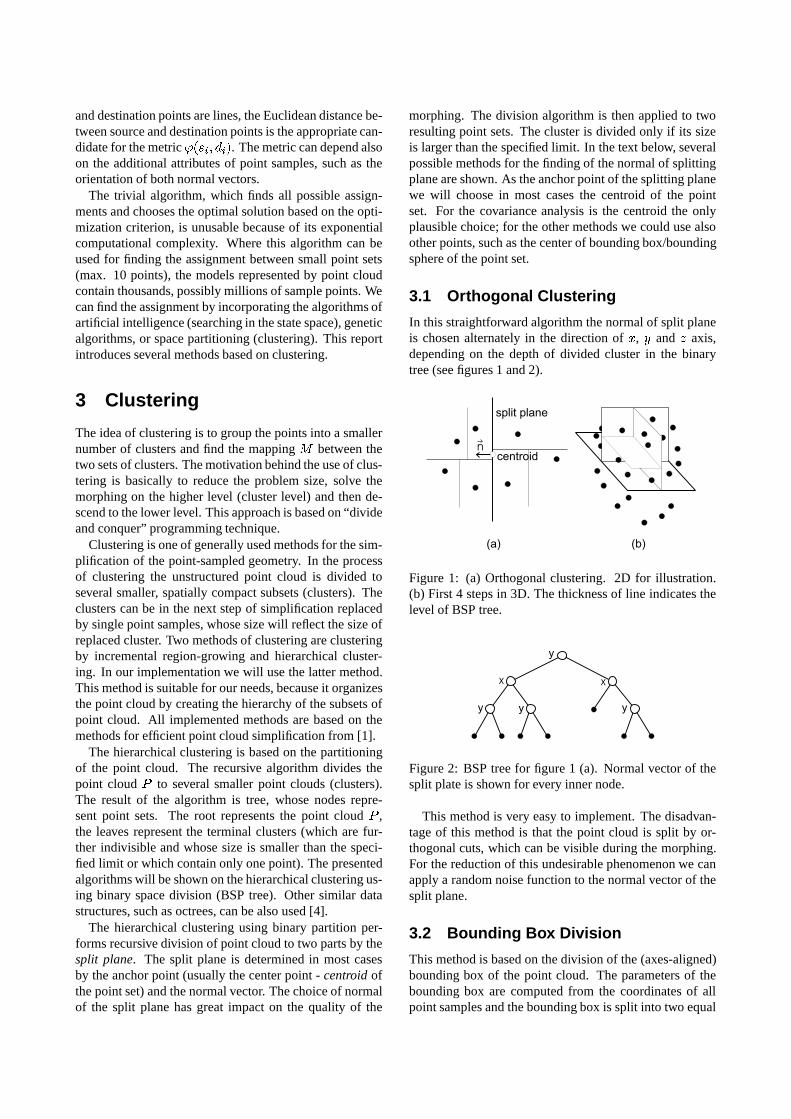
3.1 Orthogonal Clustering

In this straightforward algorithm the normal of split planeis chosen alternately in the direction of � , � and � axis,depending on the depth of divided cluster in the binarytree (see figures 1 and 2).

Figure 1: (a) Orthogonal clustering. 2D for illustration.(b) First 4 steps in 3D. The thickness of line indicates thelevel of BSP tree.

Figure 2: BSP tree for figure 1 (a). Normal vector of thesplit plate is shown for every inner node.

This method is very easy to implement. The disadvan-tage of this method is that the point cloud is split by or-thogonal cuts, which can be visible during the morphing.For the reduction of this undesirable phenomenon we canapply a random noise function to the normal vector of thesplit plane.

3.2 Bounding Box Division

This method is based on the division of the (axes-aligned)bounding box of the point cloud. The parameters of thebounding box are computed from the coordinates of allpoint samples and the bounding box is split into two equal

halves by the plane perpendicular to its longest axis. Thismethod does not necessarily involve the computation ofthe centroid for each cluster (the anchor point for the split-ting plane can be chosen as the center of the boundingbox), but we must find the dimensions and location of thebounding box. The bounding box can be specified by twopoints in 3D space, representing the lower front left andupper back right corners. This method leads to decent re-sults, compared to orthogonal clustering. However, themethod is more computationally expensive than the for-mer method, since the finding of the corners of the bound-ing box takes several times (roughly twice) more time thanthe finding of the centroid.

3.3 Covariance Analysis

The normal vector of the split plane can be found using thecovariance analysis of the neighborhood of the centroidof the point cloud. The covariance analysis allows us toestimate various local surface properties, such as normalvector of approximation surface or surface variation. Thecovariance matrix � of the point cluster � is defined as

� ����� ���� ���� � ��� �

��� ���� ����� ���� ����� ���

where�

is the centroid of point set � . Since�

issymmetric and positive semi-definite, all eigenvalues � � ,1 � � + �-2 �� $ are real-valued and the eigenvectors � � ,1 � �0+ .-2 �� $ form an orthogonal basis. The eigenvalues� � measure the variation of point set along the direction ofthe corresponding eigenvector.

If we assume that �������! ��"� G , the plane�$# � � � �%� � +minimizes the sum of squared distances to the neighborsof

�. If � is the set of points representing the surface,

then the normal �&� of this plane is the approximation ofthe normal of this surface in

�, and the plane is the pla-

nar approximation of the surface in the neighborhood of�

(tangent plane). The eigenvalue �'� expresses in this par-ticular case the variation of the surface along the normal� � , or by other words it estimates how much the points ofsurface deviate from the tangent plane. For more detaileddescription see [1].

The normal vector of the split plane will be defined bythe centroid of � and the largest eigenvector of the covari-ance matrix of � (which is � G ). The point cloud is alwayssplit along the direction of greatest variation, see the fig-ure 3.

The drawback of this method is increased computa-tional complexity (although the asymptotic complexity re-mains the same). Besides the centroid we must evaluatethe coefficients of covariance matrix

�(since the matrix

is symmetric, there are six coefficients), find the roots ofcharacteristic polynomial of

�and finally compute the

eigenvector corresponding to the largest eigenvalue.

Figure 3: (a) Clustering based on the covariance analysis.2D for illustration. (b) First 4 steps in 3D. The thicknessof line indicates the level of BSP tree.

4 Assignment of Points

The trees ( : and ( ? created by the clustering of startingand final point-cloud model in the next stage serve as in-put for the algorithm for the generation of assignments� �'� � � � � � � $ . The algorithm is pretty straightforward:in each step will be assigned one cluster from ( : to somecluster from ( ? . In the beginning the roots of both trees areassigned one to another and the assignment is put to the or-dinary queue. In the next step, the assignment �*) : +) ? � isextracted from the queue. If any of the clusters ) : , ) ? isa leaf, the assignment is put again to the queue, else thechildren of ) : and ) ? are examined, assigned to each otherand these assignments are put to the queue. This step isrepeated until the queue contains only the assignments oftype �,) : +) ? � , where at least one of ) : or ) ? represents aleaf in the corresponding tree (terminal cluster). For anexample of possible assignment see the figure 4.

Figure 4: An example of the assignment of points

The way clusters are assigned to each other depends onthe chosen metric function. Since we have defined the met-ric E only between two points (which will be in our case anEuclidean distance between two points, E � �

� � � � � � ),we have to extend the definition, so it could be applicablealso to clusters. The metric E �,- �. � between two clusters- ��( : , . �/( ? is defined as E � %!0 %'1 � , where %'0 and %'1 arecentroids of clusters - and . respectively. Let us assumethat both trees are regular with the same degree 2 (everyinternal node has exactly 2 children). During the findingof assignments of children of source node ) : to the chil-

dren of destination node ) ? we seek such permutation � of2 elements, which minimizes the following expression:58 ��� EHG � �0� � � 9 � A � where ) : ��� � � G ����� ��5 $ and ) ? � � � � G �����

� 5 $ ; �0�and

� � are children (subclusters) of nodes (clusters) ) : and) ? . This can be most easily done by trying all 2 � possibili-ties and choose the optimal. While 2 will be usually small(2 for BSP tree, 4 for quadtree or 8 for octree), this ratherbrute-force approach is an acceptable solution.

The algorithm presented above generates the set of as-signments ��H� � �,) : +) ? � $ , where ) : and ) ? are clustersfrom source and destination point clouds respectively. Weneed to generate the assignment of individual point sam-ples. This can be done by replacing the assignments be-tween clusters by the sets of assignment between points.The assignment �� � � ��� � , where � �,- +- G ����� -�� �and � � �*. �. G ����� .�� � , will be replaced by the set of �assignments �*- � �.�� � , where � ������� ��� �� � . Assumingthat ����� , this set can be described as mapping of theset � onto the set . The actual mapping we can choosedeliberately or we can apply some criteria based on metricfunction. The only important feature of this mapping isthat it should be uniform in the sense that the number ofpoints from � assigned to individual points - �#� shouldbe for all points - � approximately the same. The situationcan be simplified if we set for the clustering algorithm themaximum limit for the cluster size to 1, so the assignmentsbetween clusters will be always of type - �! or � - .4.1 Linear Interpolation

By computing the set � of the assignments between indi-vidual point samples we have reduced whole rather com-plicated problem with point cloud morphing to the triv-ial problem of morphing between the assigned point pairs.Considering the straight paths between assigned points� �0� � ��� , we can get the coordinates of the points of transi-tion point cloud % � using the linear interpolation

% � � & � � � � � )( ��� �4- � ( �)� �#" ( � � ( ��* + .- / where ( is the progress of morphing. This can be appliednot only to the coordinates, but also to other properties ofpoint samples, such as color (red, green and blue compo-nents), transparency or size. With the normal, the situa-tion is slightly more difficult. The interpolation of indi-vidual components of the normal is not optimal, becauseduring the interpolation the length of normal and the angu-lar speed of vector rotation is not constant (as it should be).The first problem can be solved by the subsequent normal-ization of normal vector. The better (and slower) solutionis to rotate the normal vector instead the interpolation ofthe components. In most cases, however, the differencesbetween results of methods which use interpolation withnormalization and rotation are negligible.

Another possible solution is to use the polar coordinatesfor normals, so instead of coordinates we have to store theangles (since all normals are unit vectors, we do not haveto store the length of vector). The linear interpolation ofangles will yield correct results. During the rendering theangles have to be transformed back to the normals. Thismethod will give the same results as the rotation of vectorsand is faster and less memory expensive (we have to storetwo angles instead of three components of normal).

5 Implementation and Testing

For the purposes of testing we have developed an applica-tion that can load two point cloud models, perform the nec-essary data preprocessing, perform the hierarchical clus-tering, generate the assignments between point pairs andvisualize the actual morphing process. Our applicationwas written in C++ using OpenGL and Qt 2.3.0 and com-piled by MSVC 6.0 under Windows. Some data structuresand the format of input files were adopted from the exist-ing application QSplat [6] (a visualization system for pointcloud models).

The implemented methods for morphing between mod-els represented by a point cloud have been tested on twentypairs of models. For some of the pairs the computationtimes of the process of finding of the assignment of pointshave been measured. The asymptotic complexity of theorthogonal clustering, the clustering based on the covari-ance analysis and the computation of the assignment of thepoints have been calculated.

The orthogonal clustering and the axes-aligned bound-ing box division have the $ � 2 &%('*)

G 2 � complexity. Theclustering based on the covariance analysis have also the$ � 2 +%('*) G 2 � complexity, they differ only in constant. Thecomputation of the assignment of the points has the $ � 2 �complexity.

The measured durations for the tested pairs of modelsare given in the table 1. Three pairs of models were tested:the sphere and the Stanford bunny (both models have thesame number of points), the African mask and the Christ-mas star, and finally the lion and the dinosaur. The mea-sured times correspond to the fact that the asymptotic com-plexities of all tested clustering methods differ only in con-stant.

We have decreased the computational complexity andthe total time spent by finding the assignments by allowingto store the once found assignments of points to file andthen load it again.

The progress of morphing of the tested pairs of modelsusing various clustering methods is shown on the figures6-10 (morphing of the sphere to the bunny), figures 11-15(morphing of the African mask to the Christmas star) andthe figures 16-20 (morphing of the lion to the dinosaur).Besides four tested clustering methods (orthogonal clus-tering, orthogonal clustering with random noise, boundingbox division, covariance analysis) there is also shown for

Models sphere-bunny mask-star lion-dinosaur� �����35 285 54 773 183 409� �����35 285 75 782 56 195

���2s 7s 16s

� ��� 2s 7s 16s

���������7s 25s 73s

�����20s 78s 302s

Table 1: Measured times

the sake of comparison the case when the assignment ofpoints is chosen randomly.

In the table 1, � is the size of the point cloud of thesource model and � G is the size of the point cloud ofthe destination model. The values (���� , (����� , (�������and (��� are the times spent by computing the assign-ment of the points for the morphing using the orthogo-nal clustering, orthogonal clustering with random noise,axes-aligned bounding box division and covariance analy-sis respectively. The values were measured on system withprocessor Athlon 1GHz and 256MB RAM.

6 Discussion

In this section we will discuss the problems that providesthe implemented methods. The main problem is the occa-sional occurrence of cracks in the model during the mor-phing. The cracks occur because of the space partitioningand the non-convexity of the shape. Our opinion is thatthis problem can not be eliminated only on the assumptionof the sum of squared distances as the criterion of qual-ity. This criterion is usable only for convex shapes. In aconvex shape every surface point can be connected withevery other surface points with a line without intersectingthe surface of the shape. If a convex shape is divided by asplit plane then the results are always two convex shapes.On the other hand a non-convex shape can be divided by asplit plane to any number of convex or non-convex shapesand this is the main reason for the occurrence of cracks,see figure 5.

Alexa et al. have presented in [3] methods for trans-formation of a non-convex B-rep shape to a convex shape.The 3D manifold objects are homeomorphic with a sphere,so the unit sphere is the convex shape on which the non-convex shapes should be transformed. Those methods canbe adapted for the point cloud representation.

One class of shapes are the star shapes. For a star shapeexist at least one point $ inside the shape which can beconnected with every boundary point of the shape witha line without intersecting the surface of the shape. Thepoint $ is called origin. If the coordinate system is trans-formed to be the origin $ in its center and the coordinatesof each boundary point normalized then the star shape hasbeen transformed to the unit sphere. The main problem isto find whether a shape is a star shape or not and find the

Figure 5: (a) The source shape. (b) The target shape. Acrack will occur because of the non-convexity of sourceshape.

origin $ , especially for point cloud representation whereno information about the surface is included.

Second class of shapes are non-convex non-star shapes.This class of shapes can be transformed to unit sphere us-ing the barycentric mapping. The barycentric mappinguses a simple idea that every point is placed in centroid ofits neighbors. The shape should be down-sampled until itis a convex shape. The coordinate system should be trans-formed to be the centroid of the shape in its center, thenthe coordinates of the points should be normalized, and thedown-sampled points should be up-sampled on unit sphererespecting the idea of barycentric mapping.

In this case the paths can not be lines. The pathsshould depend on function which transforms the non-convex shape to unit sphere.

These problems are rather non-trivial ones and the fu-ture work will be focused on these particular problems.

7 Conclusion

For convex or just a little bit non-convex models gives thebest results the morphing based on the orthogonal cluster-ing. The generally best method for non-convex models cannot be chosen. The testing has proved that the results of allmethods depend on the shapes of the source model and thetarget model.

These methods are not usable for high-quality morph-ing, so the methods have to be improved. The sum ofsquared distances can not be used as only criterion of qual-ity for non-convex shapes. Non-convex shapes have to betransformed to convex shapes.

7.1 Features� Point cloud morphing allows morphing between two

point clouds representing geometric models with dif-ferent topologies that can not be transformed easilyone to another (i.e. sphere to toroid) and even formodels, for which there is no clear notion of surface(e.g. vegetation).

� Cracks occur in the model during a morphing becauseof the space partitioning and the non-convexity of theshape.

7.2 Future Work� Transform the shapes to the unit sphere before the

clustering.

� Incorporate the topological information to algo-rithms.

References

[1] Pauly, M.; Gross, M.; Kobbelt L. P.: Efficient Sim-plification of Point-Sampled Surfaces, IEEE Visual-ization, 2002

[2] Alexa, M.; Behr, J.; Cohen-Or, D.; Levin, D.; Silva,C. T.: Computing and Rendering Point Set Surfaces,IEEE Transactions on Computer Graphic and Visu-alization, 2002

[3] Alexa, M.: Mesh Morphing STAR, Eurographics2001 State of the Art Reports, Eurographics, 2001

[4] Pfister, H.; van Baar, J.: Surfels: Surface elements asrendering primitives, In Proceedings of SIGGRAPH2000, pages 335-342, SIGGRAPH, 2000

[5] Zwicker, M.; Pfister, H.; van Baar, J.; Gross, M.: Sur-face Splatting, SIGGRAPH, 2001

[6] Rusinkiewicz, S.; Levoy, M.: QSplat: A Multires-olution Point Rendering System for Large Meshes,In Proceedings of SIGGRAPH 2000, SIGGRAPH,2000

Figure 6: Example of morphing between model of sphere and model of Stanford bunny (random assignment).

Figure 7: Example of morphing between model of sphere and model of Stanford bunny (using orthogonal clustering).

Figure 8: Example of morphing between model of sphere and model of Stanford bunny (using orthogonal clustering withrandom noise).

Figure 9: Example of morphing between model of sphere and model of Stanford bunny (using axes-aligned bounding boxdivision).

Figure 10: Example of morphing between model of sphere and model of Stanford bunny (using covariance analysis).

Figure 11: Example of morphing between model of African mask and model of Christmas star (random assignment).

Figure 12: Example of morphing between model of African mask and model of Christmas star (using orthogonal cluster-ing).

Figure 13: Example of morphing between model of African mask and model of Christmas star (using orthogonal clusteringwith random noise).

Figure 14: Example of morphing between model of African mask and model of Christmas star (using axes-alignedbounding box division).

Figure 15: Example of morphing between model of African mask and model of Christmas star (using covariance analysis).

Figure 16: Example of morphing between model of lion and model of dinosaur (random assignment).

Figure 17: Example of morphing between model of lion and model of dinosaur (using orthogonal clustering).

Figure 18: Example of morphing between model of lion and model of dinosaur (using orthogonal clustering with randomnoise).

Figure 19: Example of morphing between model of lion and model of dinosaur (using axes-aligned bounding box divi-sion).

Figure 20: Example of morphing between model of lion and model of dinosaur (using covariance analysis).