Point-set Distances for Learning Representations of 3D Point Clouds

Trung Nguyen1 Quang-Hieu Pham3 Tam Le4 Tung Pham1 Nhat Ho5 Binh-Son Hua1,21VinAI Research, Vietnam 2VinUniversity, Vietnam

3Woven Planet North America, Level 5 4RIKEN AIP, Japan 5University of Texas, Austin

Abstract

Learning an effective representation of 3D point cloudsrequires a good metric to measure the discrepancy betweentwo 3D point sets, which is non-trivial due to their irregular-ity. Most of the previous works resort to using the Chamferdiscrepancy or Earth Mover’s distance, but those metricsare either ineffective in measuring the differences betweenpoint clouds or computationally expensive. In this paper, weconduct a systematic study with extensive experiments ondistance metrics for 3D point clouds. From this study, wepropose to use sliced Wasserstein distance and its variantsfor learning representations of 3D point clouds. In addition,we introduce a new algorithm to estimate sliced Wassersteindistance that guarantees that the estimated value is closeenough to the true one. Experiments show that the slicedWasserstein distance and its variants allow the neural net-work to learn a more efficient representation compared tothe Chamfer discrepancy. We demonstrate the efficiency ofthe sliced Wasserstein metric and its variants on severaltasks in 3D computer vision including training a point cloudautoencoder, generative modeling, transfer learning, andpoint cloud registration.

1. IntroductionSince the spark of the modern artificial intelligence,

3D deep learning on point clouds has become a power-ful technique for solving recognition problems such as ob-ject classification [44, 21], object detection [43], and se-mantic segmentation [41]. Generative modeling with 3Dpoint clouds has also been studied with some promising re-sults [51, 46, 32, 22, 47, 33]. Another 3D computer visionproblem that has seen the rise of deep learning approaches ispoint cloud matching [8, 11, 10, 17]. All of these problemsshare a common task — that is to learn a robust representa-tion of 3D point clouds.

One of the most important steps in learning represen-tations of 3D point clouds is to choose a metric to mea-sure the discrepancy between two point sets. There are twopopular choices for such metric: the Chamfer divergence

and the Earth Mover’s distance (EMD) [16]. While earlierworks [16, 1] has shown that EMD performs better thanChamfer in terms of learning representations, Chamfer ismore favored [10, 52, 18, 15, 12, 19] due to its significantlylower computational cost.

In this article, we revisit the similarity metric problem in3D point cloud deep learning. We propose to use the slicedWasserstein distance (SWD) [5], which is based on project-ing the points in point clouds into a line, and its variants aseffective metrics to supervise 3D point cloud autoencoders.Compared to Chamfer divergence, SWD is more suitable forpoint cloud reconstruction, while remaining computationallyefficient (cf. Figure 1). We show that Chamfer divergenceis weaker than the EMD and sliced Wasserstein distance (cf.Lemma 1) while the EMD and sliced Wasserstein distanceare equivalent. It suggests that even when two point cloudsare close in Chamfer divergence, they may not be close ineither the EMD or sliced Wasserstein distance. Furthermore,the sliced Wasserstein distance has a computational complex-ity in the order of N logN [5], which is comparable to thatof the Chamfer divergence, while EMD has a complexityin the order of N3 [39] where N is the number of points in3D point clouds. Finally, under the standard point cloudssettings, since the dimension of points is usually three, theprojection step in sliced Wasserstein distance will only leadto small loss of information of the original point clouds. As aconsequence, the sliced Wasserstein distance possesses boththe computational and statistical advantages for point cloudlearning over Chamfer divergence and EMD. To improvethe quality of slices from SWD, we also discuss variants ofsliced Wasserstein distance, including max-sliced Wasser-stein distance [13] and the proposed adaptive sliced Wasser-stein algorithm.By conducting a case study on learning a3D point cloud auto-encoder, we provide a comprehensivebenchmark on the performance of different metrics. Theseresults align with our theoretical development. In summary,our main findings are:

• A first theoretical study about the relation betweenChamfer divergence, EMD, and sliced Wasserstein dis-tance for point cloud learning (Section 4).

10478

Figure 1: We advocate the use of sliced Wasserstein distance for training 3D point cloud autoencoders. In this example,we try to morph a sphere into a chair by optimizing two different loss functions: Chamfer discrepancy (top, red) and slicedWasserstein distance (bottom, blue). The proposed sliced Wasserstein distance only takes 1000 iterations to converge, while ittakes 50000 iterations for Chamfer discrepancy.

• A new algorithm named Adaptive-sliced Wassersteinto evaluate sliced Wasserstein distance that guaranteesthat the evaluated value is close enough to the true one(Section 4).

• An extensive evaluation of point cloud learning tasksincluding point cloud reconstruction, transfer learning,point cloud registration and generation based on Cham-fer discrepancy, EMD, sliced Wasserstein distance andits variants (Section 5).

2. Related WorkSet similarity. 3D point clouds autoencoders are usefulin a wide range of applications, such as denoising [19], 3Dmatching [55, 10, 12, 31], and generative models [16, 1].Many autoencoder architectures have been proposed in re-cent few years [1, 52, 10]. To train these autoencoders, thereare two popular choices of losses: the Chamfer discrep-ancy (CD) and Earth Mover’s distance (EMD). The Chamferdiscrepancy has been widely used in point cloud deep learn-ing [16, 1, 52].

It is known that Chamfer discrepancy (CD) is not a dis-tance that means there are two different point clouds with itsCD almost equals zero. While earlier works [16, 1] showedthat EMD is better than Chamfer in 3D point clouds recon-struction task, recent works [42] still favor Chamfer discrep-ancy due to its fast computation.

Wasserstein distance. In 2D computer vision, the family ofWasserstein distances and their sliced-based versions havebeen considered in the previous works [2, 20, 48, 14, 13, 49,29, 23]. In particular, Arjovsky et al. [2] proposed usingWasserstein as the loss function in generative adversarialnetworks (GANs) while Tolstikhin et al. [48] proposed usingthat distance for the autoencoder framework. Nevertheless,Wasserstein distances, including the EMD, have expensive

computational cost and can suffer from the curse of dimen-sionality, namely, the number of data required to train themodel will grow exponentially with the dimension. To dealwith these issues of Wasserstein distances, a line of workshas utilized the slicing approach to reduce the dimensionof the target probability measures. The notable slicing dis-tance is sliced Wasserstein distance [5]. Later, the idea ofsliced Wasserstein distance had been adapted to the autoen-coder setting [25] and domain adaptation [30]. Deshpandeet al. [14] proposed to use the max-sliced Wasserstein dis-tance, a version of sliced Wasserstein distance when we onlychoose the best direction to project the probability measures,to formulate the training loss for a generative adversarialnetwork. The follow-up work [13, 49] has an improvedprojection complexity compared to the sliced Wassersteindistance. In the recent work, Nguyen et al. [37, 38] proposeda probabilistic approach to chooses a number of importantdirections via finding an optimal measure over the projec-tions. Another direction with sliced-based distances is byreplacing the linear projections with non-linear projectionsto capture more complex geometric structures of the proba-bility measures [24]. However, to the best of our knowledge,none of such works have considered the problem of learningwith 3D point clouds yet.Notation. Let Sn−1 be the unit sphere in the n-dimensionalspace. For a metric space (Ω, d) and two probability mea-sures µ and ν on Ω, let Π(µ, ν) be the set of all joint distri-butions γ such that its marginal distributions are µ and ν,respectively. For any θ ∈ Sn−1 and any measure µ, πθ♯µdenotes the pushforward measure of µ through the mappingRθ where Rθ(x) = θ⊤x for all x.

3. BackgroundTo study the performance of different metrics for point

cloud learning, we briefly review the mathematical founda-

10479

tion of the Chamfer discrepancy and the Wasserstein dis-tance, which serve as the key building blocks in this paper.Note that in computer vision, Chamfer is often abused to bea distance. Strictly speaking, Chamfer is a pseudo-distance,not a distance [16]. Therefore, in this paper, we use the termsChamfer discrepancy or Chamfer divergence instead.

3.1. Chamfer discrepancy

In point cloud deep learning, Chamfer discrepancy hasbeen adopted for many tasks. There are some variants ofChamfer discrepancy, which we provide here for complete-ness. For any two point clouds P,Q, a common formulationof the Chamfer discrepancy between P and Q is given by:

dCD(P,Q) =1

|P |∑x∈P

miny∈Q

||x−y||22+1

|Q|∑y∈Q

minx∈P

||x−y||22.

(1)A slightly modified version of Chamfer divergence is alsoused by previous works [52, 10, 12, 3] that replaces the sumby a max function:

dMCD(P,Q) = max 1

|P |∑x∈P

miny∈Q

||x− y||22,

1

|Q|∑y∈Q

minx∈P

||x− y||22. (2)

In both definitions, the min function means that Chamferdiscrepancy only cares about the nearest neighbour of apoint rather than the distribution of those nearest points.Hence, as long as the supports of x and y are close thenthe corresponding Chamfer discrepancy between them issmall, meanwhile their corresponding distributions could bedifferent. A similar phenomenon, named Chamfer blindness,was shown in [1], pointing out that Chamfer discrepancyfails to distinguish bad sample from the true one, since it isless discriminative.

3.2. Wasserstein distance

Let (Ω, d) be a metric space, µ, ν are probability mea-sures on Ω. For p ≥ 1, the p-Wasserstein distance (WD) isgiven by

Wp(µ, ν) = infγ∈Π(µ,ν)

E(X,Y )∼γ

[dp(X,Y )

] 1p

.

For p = 1, the Wasserstein distance becomes the EarthMover’s Distance (EMD), where the optimal joint distribu-tion γ induces a map T : µ → ν, which preserves the mea-sure on any measurable set B ⊂ Ω. In the one-dimensionalcase Ω = R and d(x, y) := |x− y|, the WD has the follow-ing closed-form formula:

Wp(µ, ν) =(∫ 1

0

∣∣F−1X (t)− F−1

Y (t)∣∣p, dt) 1

p

, (3)

where FX and FY are respectively the cumulative distri-bution functions of random variables X and Y . When thedimension is greater than one, there is no closed-form forthe WD, that makes calculating the WD more difficult.

EMD in 3D point-cloud applications. For the specific set-tings of 3D point clouds, the EMD had also been employedto define a metric between two point clouds [16, 1, 53]. Withan abuse of notation, for any two given point clouds P andQ, throughout this paper, we denote its measure representa-tion as follows: P = 1

|P |∑

x∈P δx and Q = 1|Q|

∑y∈Q δy

where δx denotes the Dirac delta distribution at point x inthe point cloud P . When |P | = |Q|, the Earth Mover’sdistance [16, 1, 53] between P and Q is defined as

dEMD(P,Q) = minT :P→Q

∑x∈P

||x− T (x)||2. (4)

While earlier works [16, 1] showed that EMD is better thanChamfer in 3D point clouds reconstruction task, the com-putation of EMD can be very expensive compared to theChamfer divergence. In particular, it had been shown thatthe practical computational efficiency of EMD is at the orderof max|P |, |Q|3 [39], which can be expensive. There is arecent line of work using entropic version of EMD or in gen-eral Wasserstein distances [9] to speed up the computationof EMD. However, the best known practical complexity ofusing the entropic approach for approximating the EMD is atthe order max|P |, |Q|2 [34, 35], which is still expensiveand slower than that of Chamfer divergence. Therefore, it ne-cessitates to develop a metric between 3D point clouds suchthat it not only has equivalent statistical properties as thoseof EMD but also has favorable computational complexitysimilar to that of the Chamfer divergence.

4. Sliced Wasserstein Distance and its variantsIn this section, we first show that Chamfer divergence

is a weaker divergence than Earth Mover’s distance in Sec-tion 4.1. Since Earth Mover’s distance can be expensiveto compute, we propose using sliced Wasserstein distance,which is equivalent to Wasserstein distance and has effi-cient computation, as an alternative to EMD in Section 4.2.1.Finally, we propose a new algorithm to compute sliced-Wasserstein that can guarantee the estimated value is closeenough to the true one in Section 4.2.2.

4.1. Relation between Chamfer divergence andEarth Mover’s distance

In this section, we study the relation between Chamferand EMD when |P | = |Q|. In particular, the followinginequality shows that the Chamfer divergence is weaker thanthe Wasserstein distance.

Lemma 1. Assume |P | = |Q| and the support of P and Qis bounded in a convex hull of diameter K, then we find that

10480

dCD(P,Q) ≤ 2KdEMD(P,Q). (5)

Proof. Assume that T is the optimal plan from P to Q. Then,we find that

miny∈Q

∥x− y∥2 ≤ ∥x− T (x)∥2

⇒ miny∈Q

∥x− y∥22 ≤ K∥x− T (x)∥2,

since ∥x− T (x)∥2 ≤ K. Taking the sum over x, we obtain

∑x∈P

miny∈Q

∥x− y∥22 ≤ K∑x∈P

∥x− T (x)∥2.

Similarly we have∑

y∈Q minx∈P ∥x − y∥22 ≤K

∑y∈Q ∥y − T (y)∥2 where T is the optimal plan

from Q to P . Then we obtain the desired inequality.

The inequality in Lemma 1 implies that minimizing theWasserstein distance leads to a smaller Chamfer discrepancy,and the reverse inequality is not true. Therefore, EMD andChamfer divergence are not equivalent, which can be unde-sirable. Note that the inequality could not be improved toa better order of K. For example, lets consider two point-clouds that have small variance ϵ2, meanwhile the distancebetween two point-cloud centers equals K −O(ϵ). Then theCD is of order K2, the EMD is of order K.

Lemma 1 shows that Chamfer divergence is weaker thanthe EMD, which is in turn weaker than other divergencessuch as, KL, chi-squared, etc. [40, pp.117]. However, Cham-fer discrepancy has weakness as we explained before, andother divergences are not as effective as EMD, since theyare very loose even when two distributions are close to eachother [2]. Hence, the Wasserstein/EMD is a preferable metricfor learning the discrepancy between two distributions.

Despite that fact, computing EMD can be quite expen-sive since it is equivalent to solving a linear programmingproblem, which has the best practical computational com-plexity of the order O(max|P |3, |Q|3) [39]. On the otherhand, the computational complexity of Chamfer divergencecan be scaled up to the order O(max|P |, |Q|). Therefore,Chamfer divergence is still preferred in practice due to itsfavorable computational complexity.

Given the above observation, ideally, we would like toutilize a distance between P and Q such that it is equiva-lent to the EMD and has linear computational complexity interms of max|P |, |Q|, which is comparable to the Cham-fer divergence. It leads us to the notion of sliced Wassersteindistance in the next section.

4.2. Sliced Wasserstein distance and its variants

In order to circumvent the high computational complexityof EMD, the sliced Wasserstein distance [5] is designedto exploit the 1D formulation of Wasserstein distance inEquation (3).

4.2.1 Sliced Wasserstein distance

In particular, the idea of sliced Wasserstein distance is thatwe first project both target probability measures µ and ν ona direction, says θ, on the unit sphere to obtain two projectedmeasures denoted by πθ♯µ and πθ♯ν, respectively. Then,we compute the Wasserstein distance between two projectedmeasures πθ♯µ and πθ♯ν. The sliced Wasserstein distance(SWD) is defined by taking the average of the Wassersteindistance between the two projected measures over all possi-ble projected direction θ. In particular, for any given p ≥ 1,the sliced Wasserstein distance of order p is formulated asfollows:

SWp(µ, ν) =(∫

Sn−1

W pp

(πθ♯µ, πθ♯ν)dθ

) 1p

. (6)

The SWp is considered as a low-cost approximation forWasserstein distance as its computational complexity is ofthe order O(n log n) where n is the maximum number ofsupports of the discrete probability measures µ and ν. Whenp = 1, the SWp is weakly equivalent to first order WD orequivalently EMD [4]. The equivalence between SW1 andEMD along with the result of Lemma 1 suggests that SW1 isstronger metric than the Chamfer divergence while it has anappealing optimal computational complexity that is linear onthe number of points of point clouds, which is comparableto that of Chamfer divergence.

We would like to remark that since the dimension ofpoints in point clouds is generally small (≤ 6), sliced Wasser-stein distance will still be able to retain useful information ofthe point clouds even after we project them to some directionon the sphere. Due to its favorable computational complexity,sliced Wasserstein distance had been used in several appli-cations: point cloud registration [28], generative models on2D images; see, for examples [45, 36, 14, 25, 26, 49, 27].However, to the best of our knowledge, this distance has notbeen used for deep learning tasks on 3D point clouds.

Monte Carlo estimation. In Equation (6), the integral isgenerally intractable to compute. Therefore, we need toapproximate the integral. A common approach to approx-imate the integral is by applying the Monte Carlo method.In particular, we sample N directions θ1, . . . , θN uniformlyfrom the sphere Sd−1 where d is the dimension of points inpoint clouds, which results in the following approximation

10481

of sliced Wasserstein distance:

SWp(µ, ν) ≈( 1

N

N∑i=1

W pp

(πθi♯µ, πθi♯ν

)) 1p

. (7)

where the number of slices N is tuned for the best perfor-mance.

Since N plays a key role in determining the approxima-tion of sliced Wasserstein distance, it is usually chosen basedon the dimension of the probability measures µ and ν. In ourapplications with 3D point clouds, since the dimension ofthe points in point clouds is generally small, we observe thatchoosing the number of projections N up to 100 is alreadysufficient for learning 3D point clouds well.

Max-sliced Wasserstein distance. To avoid using uninfor-mative slices in SWD, another approach focuses on takingonly the best slice in discriminating between two given distri-butions. That results in max-sliced Wasserstein distance [13].For any p ≥ 1, the max-sliced Wasserstein distance of orderp is given by:

MSWp(µ, ν) := maxθ∈Sn−1

Wp

(πθ♯µ, πθ♯ν). (8)

4.2.2 An adaptive-sliced Wasserstein algorithm

Another drawback of the Monte Carlo estimation in SWDis that it does not give information about how close the esti-mated value is to the true one. Therefore, we introduce thenovel adaptive-sliced Wasserstein algorithm (ASW). In par-ticular, given N uniform random projections θiN1 drawnfrom the sphere Sn−1, for the simplicity of presentation, wedenote swi = W p

p

(πθi♯µ, πθi♯ν) for all 1 ≤ i ≤ N . Fur-

thermore, we denote sw = SW pp (µ, ν) the true value of

SW distance that we want to compute. The Monte Carloestimation of the SW distance can be written as follows:swN := 1

N

∑Ni=1 swi, which is an unbiased estimator of the

true value sw. Similarly, the biased and unbiased varianceestimates are respectively defined as:

s2N :=1

N

N∑i=1

(swi − swN

)2, s2N :=

N

N − 1s2N . (9)

Our idea of adaptivity is to dynamically determine the num-ber of projections N from the observed mean and variance ofthe estimators. To do so, we leverage a probabilistic boundof the error of the estimator and choose N such that the errorbound is below a certain tolerance threshold. Particularly,applying central limit theorem, we have

P(|swN − sw| < ksN√

N

)≈ ϕ(k)− ϕ(−k) (10)

where ϕ(k) :=∫ k

−∞e−x2/2√2π

dx. We set k = 2 so that theabove probability is around 95%.

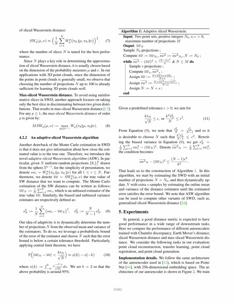
Algorithm 1: Adaptive sliced Wasserstein.Input: Two point sets, positive integers N0, s; ϵ > 0;

maximum number of projections MOuput: swN

Sample N0 projections ;Compute sw := swN0

, sw2 := sw2N0

, N := N0 ;

while sw2 − (sw)2 > (N−1)ϵ2

4 & N ≤ M doSample s projections ;Compute sws, sw2

s ;Assign sw := N×sw+s×sws

N+s ;

Assign sw2 := N×sw2+s×sw2s

N+s ;Assign N := N + s ;

end

Given a predefined tolerance ϵ > 0, we aim for

ksN√N

≤ ϵ, ork2s2NN

≤ ϵ2. (11)

From Equation (9), we note that s2NN =

s2NN−1 and so it

is desirable to choose N such that k2s2NN−1 ≤ ϵ2. Rewrit-

ing the biased variance in Equation (9), we get s2N =1N

∑Ni=1 sw

2i − (swN )2. Denote sw2

N := 1N

∑Ni=1 sw

2i ,

the condition becomes

sw2N − (swN )2 ≤ (N − 1)ϵ2

k2.

That leads us to the construction of Algorithm 1. In thisalgorithm, we start by estimating the SWD with an initialnumber of projections N = N0, and then dynamically up-date N with extra s samples by estimating the online meanand variance of the distance estimator until the estimatederror satisfies the error bound. We note that ASW algorithmcan be used to compute other variants of SWD, such as,generalized sliced-Wasserstein distance [24].

5. ExperimentsIn general, a good distance metric is expected to have

good performance in a wide range of downstream tasks.Here we compare the performance of different autoencoderstrained with Chamfer discrepancy, Earth Mover’s distance,sliced Wasserstein distance and max-sliced Wasserstein dis-tance. We consider the following tasks in our evaluation:point cloud reconstruction, transfer learning, point cloudregistration, and point cloud generation.

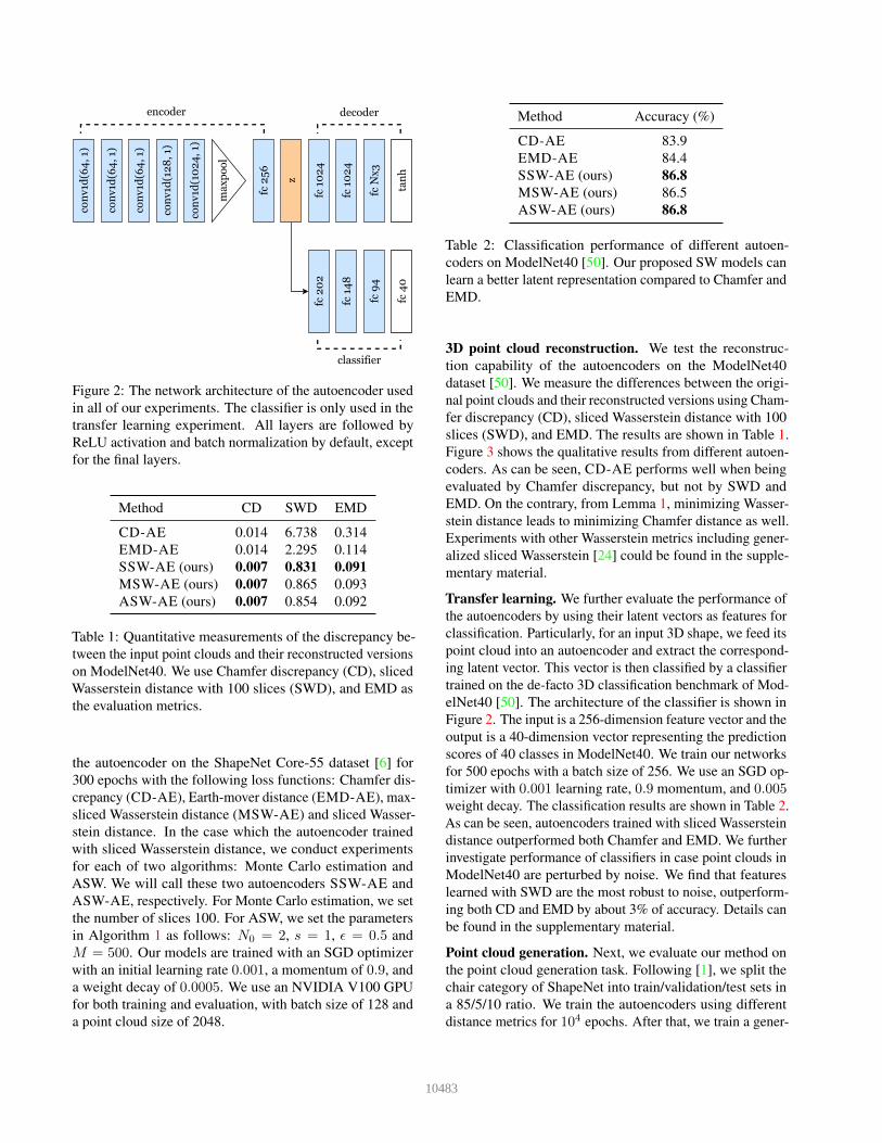
Implementation details. We follow the same architectureof the autoencoder used in [42], which is based on Point-Net [44], with 256-dimensional embedding space. The ar-chitecture of our autoencoder is shown in Figure 2. We train

10482

conv1d(64,1)

conv1d(64,1)

conv1d(64,1)

conv1d(128,1)

conv1d(1024,1)

maxpool

fc256 z

fc1024

fc1024

fcNx3

tanh

fc94

fc40

fc148

fc202

encoder decoder

classifier

Figure 2: The network architecture of the autoencoder usedin all of our experiments. The classifier is only used in thetransfer learning experiment. All layers are followed byReLU activation and batch normalization by default, exceptfor the final layers.

Method CD SWD EMD

CD-AE 0.014 6.738 0.314EMD-AE 0.014 2.295 0.114SSW-AE (ours) 0.007 0.831 0.091MSW-AE (ours) 0.007 0.865 0.093ASW-AE (ours) 0.007 0.854 0.092

Table 1: Quantitative measurements of the discrepancy be-tween the input point clouds and their reconstructed versionson ModelNet40. We use Chamfer discrepancy (CD), slicedWasserstein distance with 100 slices (SWD), and EMD asthe evaluation metrics.

the autoencoder on the ShapeNet Core-55 dataset [6] for300 epochs with the following loss functions: Chamfer dis-crepancy (CD-AE), Earth-mover distance (EMD-AE), max-sliced Wasserstein distance (MSW-AE) and sliced Wasser-stein distance. In the case which the autoencoder trainedwith sliced Wasserstein distance, we conduct experimentsfor each of two algorithms: Monte Carlo estimation andASW. We will call these two autoencoders SSW-AE andASW-AE, respectively. For Monte Carlo estimation, we setthe number of slices 100. For ASW, we set the parametersin Algorithm 1 as follows: N0 = 2, s = 1, ϵ = 0.5 andM = 500. Our models are trained with an SGD optimizerwith an initial learning rate 0.001, a momentum of 0.9, anda weight decay of 0.0005. We use an NVIDIA V100 GPUfor both training and evaluation, with batch size of 128 anda point cloud size of 2048.

Method Accuracy (%)

CD-AE 83.9EMD-AE 84.4SSW-AE (ours) 86.8MSW-AE (ours) 86.5ASW-AE (ours) 86.8

Table 2: Classification performance of different autoen-coders on ModelNet40 [50]. Our proposed SW models canlearn a better latent representation compared to Chamfer andEMD.

3D point cloud reconstruction. We test the reconstruc-tion capability of the autoencoders on the ModelNet40dataset [50]. We measure the differences between the origi-nal point clouds and their reconstructed versions using Cham-fer discrepancy (CD), sliced Wasserstein distance with 100slices (SWD), and EMD. The results are shown in Table 1.Figure 3 shows the qualitative results from different autoen-coders. As can be seen, CD-AE performs well when beingevaluated by Chamfer discrepancy, but not by SWD andEMD. On the contrary, from Lemma 1, minimizing Wasser-stein distance leads to minimizing Chamfer distance as well.Experiments with other Wasserstein metrics including gener-alized sliced Wasserstein [24] could be found in the supple-mentary material.

Transfer learning. We further evaluate the performance ofthe autoencoders by using their latent vectors as features forclassification. Particularly, for an input 3D shape, we feed itspoint cloud into an autoencoder and extract the correspond-ing latent vector. This vector is then classified by a classifiertrained on the de-facto 3D classification benchmark of Mod-elNet40 [50]. The architecture of the classifier is shown inFigure 2. The input is a 256-dimension feature vector and theoutput is a 40-dimension vector representing the predictionscores of 40 classes in ModelNet40. We train our networksfor 500 epochs with a batch size of 256. We use an SGD op-timizer with 0.001 learning rate, 0.9 momentum, and 0.005weight decay. The classification results are shown in Table 2.As can be seen, autoencoders trained with sliced Wassersteindistance outperformed both Chamfer and EMD. We furtherinvestigate performance of classifiers in case point clouds inModelNet40 are perturbed by noise. We find that featureslearned with SWD are the most robust to noise, outperform-ing both CD and EMD by about 3% of accuracy. Details canbe found in the supplementary material.

Point cloud generation. Next, we evaluate our method onthe point cloud generation task. Following [1], we split thechair category of ShapeNet into train/validation/test sets ina 85/5/10 ratio. We train the autoencoders using differentdistance metrics for 104 epochs. After that, we train a gener-

10483

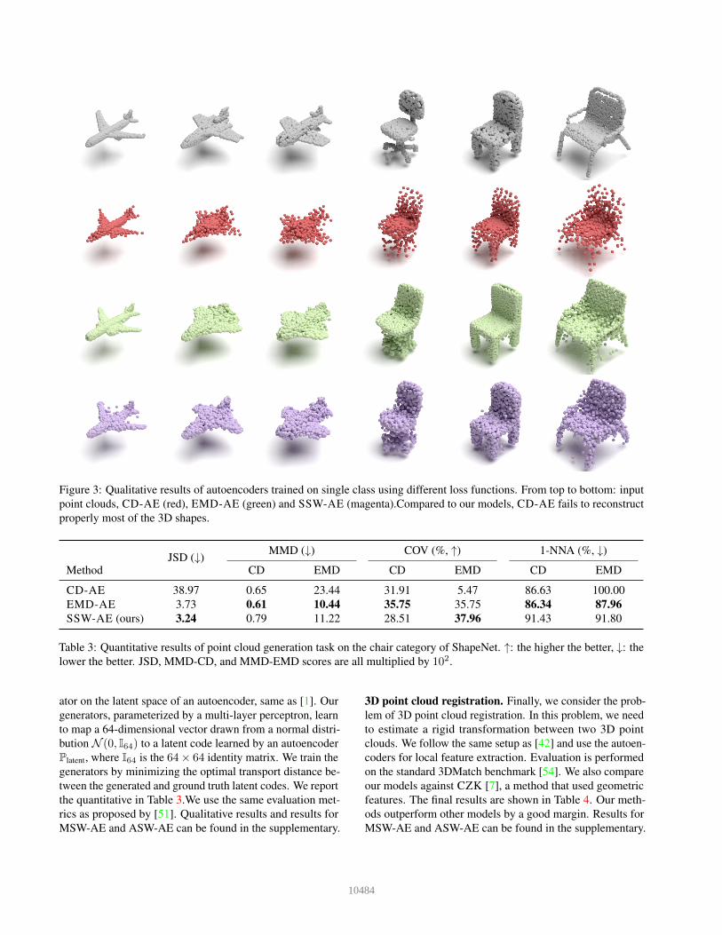
Figure 3: Qualitative results of autoencoders trained on single class using different loss functions. From top to bottom: inputpoint clouds, CD-AE (red), EMD-AE (green) and SSW-AE (magenta).Compared to our models, CD-AE fails to reconstructproperly most of the 3D shapes.

JSD (↓) MMD (↓) COV (%, ↑) 1-NNA (%, ↓)

Method CD EMD CD EMD CD EMD

CD-AE 38.97 0.65 23.44 31.91 5.47 86.63 100.00EMD-AE 3.73 0.61 10.44 35.75 35.75 86.34 87.96SSW-AE (ours) 3.24 0.79 11.22 28.51 37.96 91.43 91.80

Table 3: Quantitative results of point cloud generation task on the chair category of ShapeNet. ↑: the higher the better, ↓: thelower the better. JSD, MMD-CD, and MMD-EMD scores are all multiplied by 102.

ator on the latent space of an autoencoder, same as [1]. Ourgenerators, parameterized by a multi-layer perceptron, learnto map a 64-dimensional vector drawn from a normal distri-bution N (0, I64) to a latent code learned by an autoencoderPlatent, where I64 is the 64× 64 identity matrix. We train thegenerators by minimizing the optimal transport distance be-tween the generated and ground truth latent codes. We reportthe quantitative in Table 3.We use the same evaluation met-rics as proposed by [51]. Qualitative results and results forMSW-AE and ASW-AE can be found in the supplementary.

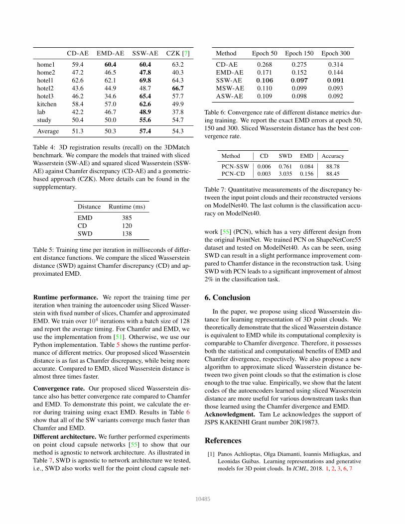
3D point cloud registration. Finally, we consider the prob-lem of 3D point cloud registration. In this problem, we needto estimate a rigid transformation between two 3D pointclouds. We follow the same setup as [42] and use the autoen-coders for local feature extraction. Evaluation is performedon the standard 3DMatch benchmark [54]. We also compareour models against CZK [7], a method that used geometricfeatures. The final results are shown in Table 4. Our meth-ods outperform other models by a good margin. Results forMSW-AE and ASW-AE can be found in the supplementary.

10484

CD-AE EMD-AE SSW-AE CZK [7]

home1 59.4 60.4 60.4 63.2home2 47.2 46.5 47.8 40.3hotel1 62.6 62.1 69.8 64.3hotel2 43.6 44.9 48.7 66.7hotel3 46.2 34.6 65.4 57.7kitchen 58.4 57.0 62.6 49.9lab 42.2 46.7 48.9 37.8study 50.4 50.0 55.6 54.7

Average 51.3 50.3 57.4 54.3

Table 4: 3D registration results (recall) on the 3DMatchbenchmark. We compare the models that trained with slicedWasserstein (SW-AE) and squared sliced Wasserstein (SSW-AE) against Chamfer discrepancy (CD-AE) and a geometric-based approach (CZK). More details can be found in thesuppplementary.

Distance Runtime (ms)

EMD 385CD 120SWD 138

Table 5: Training time per iteration in milliseconds of differ-ent distance functions. We compare the sliced Wassersteindistance (SWD) against Chamfer discrepancy (CD) and ap-proximated EMD.

Runtime performance. We report the training time periteration when training the autoencoder using Sliced Wasser-stein with fixed number of slices, Chamfer and approximatedEMD. We train over 104 iterations with a batch size of 128and report the average timing. For Chamfer and EMD, weuse the implementation from [51]. Otherwise, we use ourPython implementation. Table 5 shows the runtime perfor-mance of different metrics. Our proposed sliced Wassersteindistance is as fast as Chamfer discrepancy, while being moreaccurate. Compared to EMD, sliced Wasserstein distance isalmost three times faster.

Convergence rate. Our proposed sliced Wasserstein dis-tance also has better convergence rate compared to Chamferand EMD. To demonstrate this point, we calculate the er-ror during training using exact EMD. Results in Table 6show that all of the SW variants converge much faster thanChamfer and EMD.Different architecture. We further performed experimentson point cloud capsule networks [55] to show that ourmethod is agnostic to network architecture. As illustrated inTable 7, SWD is agnostic to network architecture we tested,i.e., SWD also works well for the point cloud capsule net-

Method Epoch 50 Epoch 150 Epoch 300

CD-AE 0.268 0.275 0.314EMD-AE 0.171 0.152 0.144SSW-AE 0.106 0.097 0.091MSW-AE 0.110 0.099 0.093ASW-AE 0.109 0.098 0.092

Table 6: Convergence rate of different distance metrics dur-ing training. We report the exact EMD errors at epoch 50,150 and 300. Sliced Wasserstein distance has the best con-vergence rate.

Method CD SWD EMD Accuracy

PCN-SSW 0.006 0.761 0.084 88.78PCN-CD 0.003 3.035 0.156 88.45

Table 7: Quantitative measurements of the discrepancy be-tween the input point clouds and their reconstructed versionson ModelNet40. The last column is the classification accu-racy on ModelNet40.

work [55] (PCN), which has a very different design fromthe original PointNet. We trained PCN on ShapeNetCore55dataset and tested on ModelNet40. As can be seen, usingSWD can result in a slight performance improvement com-pared to Chamfer distance in the reconstruction task. UsingSWD with PCN leads to a significant improvement of almost2% in the classification task.

6. Conclusion

In the paper, we propose using sliced Wasserstein dis-tance for learning representation of 3D point clouds. Wetheoretically demonstrate that the sliced Wasserstein distanceis equivalent to EMD while its computational complexity iscomparable to Chamfer divergence. Therefore, it possessesboth the statistical and computational benefits of EMD andChamfer divergence, respectively. We also propose a newalgorithm to approximate sliced Wasserstein distance be-tween two given point clouds so that the estimation is closeenough to the true value. Empirically, we show that the latentcodes of the autoencoders learned using sliced Wassersteindistance are more useful for various downstream tasks thanthose learned using the Chamfer divergence and EMD.Acknowledgment. Tam Le acknowledges the support ofJSPS KAKENHI Grant number 20K19873.

References[1] Panos Achlioptas, Olga Diamanti, Ioannis Mitliagkas, and

Leonidas Guibas. Learning representations and generativemodels for 3D point clouds. In ICML, 2018. 1, 2, 3, 6, 7

10485

[2] Martin Arjovsky, Soumith Chintala, and Leon Bottou. Wasser-stein generative adversarial networks. In ICML, pages 214–223, 2017. 2, 4

[3] Tristan Aumentado-Armstrong, Stavros Tsogkas, Allan Jep-son, and Sven Dickinson. Geometric disentanglement forgenerative latent shape models. In ICCV, 2019. 3

[4] Erhan Bayraktar and Gaoyue Guo. Strong equivalencebetween metrics of Wasserstein type. arXiv preprintarXiv:1912.08247, 2019. 4

[5] Nicolas Bonneel, Julien Rabin, Gabriel Peyre, and HanspeterPfister. Sliced and Radon Wasserstein barycenters of mea-sures. Journal of Mathematical Imaging and Vision, 1(51):22–45, 2015. 1, 2, 4

[6] Angel X Chang, Thomas Funkhouser, Leonidas Guibas,Pat Hanrahan, Qixing Huang, Zimo Li, Silvio Savarese,Manolis Savva, Shuran Song, Hao Su, et al. ShapeNet:An information-rich 3D model repository. arXiv preprintarXiv:1512.03012, 2015. 6

[7] Sungjoon Choi, Qian-Yi Zhou, and Vladlen Koltun. Robustreconstruction of indoor scenes. In CVPR, 2015. 7, 8

[8] Christopher Choy, Jaesik Park, and Vladlen Koltun. Fullyconvolutional geometric features. In ICCV, 2019. 1

[9] Marco Cuturi. Sinkhorn distances: Lightspeed computationof optimal transport. In NeurIPS, pages 2292–2300, 2013. 3

[10] Haowen Deng, Tolga Birdal, and Slobodan Ilic. PPF-FoldNet:Unsupervised learning of rotation invariant 3D local descrip-tors. In ECCV, 2018. 1, 2, 3

[11] Haowen Deng, Tolga Birdal, and Slobodan Ilic. PPFNet:Global context aware local features for robust 3D point match-ing. In CVPR, 2018. 1

[12] Haowen Deng, Tolga Birdal, and Slobodan Ilic. 3D localfeatures for direct pairwise registration. In CVPR, pages3244–3253, 2019. 1, 2, 3

[13] Ishan Deshpande, Yuan-Ting Hu, Ruoyu Sun, Ayis Pyrros,Nasir Siddiqui, Sanmi Koyejo, Zhizhen Zhao, David Forsyth,and Alexander G. Schwing. Max-sliced wasserstein distanceand its use for gans. In CVPR, June 2019. 1, 2, 5

[14] Ishan Deshpande, Ziyu Zhang, and Alexander G. Schwing.Generative modeling using the sliced wasserstein distance. InCVPR, June 2018. 2, 4

[15] Chaojing Duan, Siheng Chen, and Jelena Kovacevic. 3Dpoint cloud denoising via deep neural network based localsurface estimation. In ICASSP, 2019. 1

[16] Haoqiang Fan, Hao Su, and Leonidas J Guibas. A point setgeneration network for 3D object reconstruction from a singleimage. In CVPR, 2017. 1, 2, 3

[17] Zan Gojcic, Caifa Zhou, Jan D Wegner, and Andreas Wieser.The perfect match: 3D point cloud matching with smootheddensities. In CVPR, 2019. 1

[18] Thibault Groueix, Matthew Fisher, Vladimir G Kim, Bryan CRussell, and Mathieu Aubry. A papier-mache approach tolearning 3d surface generation. In CVPR, 2018. 1

[19] Pedro Hermosilla, Tobias Ritschel, and Timo Ropinski. Totaldenoising: Unsupervised learning of 3D point cloud cleaning.In ICCV, 2019. 1, 2

[20] Nhat Ho, XuanLong Nguyen, Mikhail Yurochkin, Hung HaiBui, Viet Huynh, and Dinh Phung. Multilevel clustering viaWasserstein means. In ICML, pages 1501–1509, 2017. 2

[21] Binh-Son Hua, Minh-Khoi Tran, and Sai-Kit Yeung. Point-wise convolutional neural networks. In CVPR, 2018. 1

[22] Le Hui, Rui Xu, Jin Xie, Jianjun Qian, and Jian Yang. Pro-gressive point cloud deconvolution generation network. InECCV, 2020. 1

[23] Viet Huynh, Nhat Ho, Nhan Dam, Long Nguyen, MikhailYurochkin, Hung Bui, and Dinh Phung. On efficient multi-level clustering via Wasserstein distances. Journal of MachineLearning Research, pages 1–43, 2021. 2

[24] Soheil Kolouri, Kimia Nadjahi, Umut Simsekli, RolandBadeau, and Gustavo Rohde. Generalized sliced wassersteindistances. In NeurIPS, 2019. 2, 5, 6

[25] Soheil Kolouri, Phillip E. Pope, Charles E. Martin, and Gus-tavo K. Rohde. Sliced Wasserstein auto-encoders. In ICLR,2019. 2, 4

[26] Soheil Kolouri, Gustavo K. Rohde, and Heiko Hoffmann.Sliced wasserstein distance for learning gaussian mixturemodels. In CVPR, June 2018. 4

[27] Soheil Kolouri, Yang Zou, and Gustavo K. Rohde. Slicedwasserstein kernels for probability distributions. In CVPR,June 2016. 4

[28] Rongjie Lai and Hongkai Zhao. Multi-scale non-rigid pointcloud registration using robust sliced-wasserstein distance vialaplace-beltrami eigenmap. arXiv preprint arXiv: 1406.3758,2014. 4

[29] Trung Le, Tuan Nguyen, Nhat Ho, Hung Bui, and Dinh Phung.LAMDA: Label matching deep domain adaptation. In ICML,2021. 2

[30] Chen-Yu Lee, Tanmay Batra, Mohammad Haris Baig, andDaniel Ulbricht. Sliced wasserstein discrepancy for unsuper-vised domain adaptation. In CVPR, June 2019. 2

[31] Chun-Liang Li, Tomas Simon, Jason Saragih, Barnabas Poc-zos, and Yaser Sheikh. Lbs autoencoder: Self-supervisedfitting of articulated meshes to point clouds. In CVPR, June2019. 2

[32] Chun-Liang Li, Manzil Zaheer, Yang Zhang, Barnabas Poc-zos, and Ruslan Salakhutdinov. Point cloud GAN. arXivpreprint arXiv:1810.05795, 2018. 1

[33] Chen-Hsuan Lin, Chen Kong, and Simon Lucey. Learningefficient point cloud generation for dense 3D object recon-struction. In AAAI, 2018. 1

[34] Tianyi Lin, Nhat Ho, and Michael Jordan. On efficient opti-mal transport: An analysis of greedy and accelerated mirrordescent algorithms. In ICML, pages 3982–3991, 2019. 3

[35] Tianyi Lin, Nhat Ho, and Michael I. Jordan. On the efficiencyof Sinkhorn and Greenkhorn and their acceleration for optimaltransport. arXiv preprint arXiv: 1906.01437, 2019. 3

[36] Kimia Nadjahi, Alain Durmus, Umut Simsekli, and RolandBadeau. Asymptotic guarantees for learning generative mod-els with the sliced-wasserstein distance. In NeurIPS, pages250–260, 2019. 4

[37] Khai Nguyen, Nhat Ho, Tung Pham, and Hung Bui. Dis-tributional sliced-Wasserstein and applications to generativemodeling. In ICLR, 2021. 2

[38] Khai Nguyen, Son Nguyen, Nhat Ho, Tung Pham, and HungBui. Improving relational regularized autoencoders withspherical sliced fused Gromov Wasserstein. In ICLR, 2021. 2

10486

[39] O. Pele and M. Werman. Fast and robust earth mover’s dis-tance. In ICCV, 2009. 1, 3, 4

[40] Gabriel Peyre and Marco Cuturi. Computational optimaltransport, 2020. 4

[41] Quang-Hieu Pham, Duc Thanh Nguyen, Binh-Son Hua,Gemma Roig, and Sai-Kit Yeung. JSIS3D: Joint semantic-instance segmentation of 3D point clouds with multi-taskpointwise networks and multi-value conditional random fields.In CVPR, 2019. 1

[42] Quang-Hieu Pham, Mikaela Angelina Uy, Binh-Son Hua,Duc Thanh Nguyen, Gemma Roig, and Sai-Kit Yeung. LCD:Learned cross-domain descriptors for 2D-3D matching. InAAAI, 2020. 2, 5, 7

[43] Charles R Qi, Or Litany, Kaiming He, and Leonidas J Guibas.Deep hough voting for 3d object detection in point clouds. InCVPR, 2019. 1

[44] Charles R Qi, Hao Su, Kaichun Mo, and Leonidas J Guibas.PointNet: Deep learning on point sets for 3D classificationand segmentation. In CVPR, 2017. 1, 5

[45] Mark Rowland, Jiri Hron, Yunhao Tang, Krzysztof Choroman-ski, Tamas Sarlos, and Adrian Weller. Orthogonal estimationof wasserstein distances. In AISTATS, 2019. 4

[46] Dong Wook Shu, Sung Woo Park, and Junseok Kwon. 3Dpoint cloud generative adversarial network based on tree struc-tured graph convolutions. In ICCV, 2019. 1

[47] Yongbin Sun, Yue Wang, Ziwei Liu, Joshua Siegel, and San-jay Sarma. PointGrow: Autoregressively learned point cloudgeneration with self-attention. In WACV, 2020. 1

[48] Ilya Tolstikhin, Olivier Bousquet, Sylvain Gelly, and Bern-hard Schoelkopf. Wasserstein auto-encoders. In ICLR, 2018.2

[49] Jiqing Wu, Zhiwu Huang, Dinesh Acharya, Wen Li, JanineThoma, Danda Pani Paudel, and Luc Van Gool. Sliced wasser-stein generative models. In CVPR, 2019. 2, 4

[50] Zhirong Wu, Shuran Song, Aditya Khosla, Fisher Yu, Lin-guang Zhang, Xiaoou Tang, and Jianxiong Xiao. 3DShapeNets: A deep representation for volumetric shapes. InCVPR, 2015. 6

[51] Guandao Yang, Xun Huang, Zekun Hao, Ming-Yu Liu, SergeBelongie, and Bharath Hariharan. PointFlow: 3D point cloudgeneration with continuous normalizing flows. In ICCV, 2019.1, 7, 8

[52] Yaoqing Yang, Chen Feng, Yiru Shen, and Dong Tian. Fold-ingNet: Point cloud auto-encoder via deep grid deformation.In CVPR, 2018. 1, 2, 3

[53] Lequan Yu, Xianzhi Li, Chi-Wing Fu, Daniel Cohen-Or, andPheng-Ann Heng. PU-Net: Point cloud upsampling network.In CVPR, 2018. 3

[54] Andy Zeng, Shuran Song, Matthias Nießner, Matthew Fisher,Jianxiong Xiao, and Thomas Funkhouser. 3DMatch: Learn-ing local geometric descriptors from RGB-D reconstructions.In CVPR, 2017. 7

[55] Yongheng Zhao, Tolga Birdal, Haowen Deng, and FedericoTombari. 3D point capsule networks. In CVPR, 2019. 2, 8

10487