poisson intensity estimation with reproducing kernels · poisson intensity estimation with ......

Vol. 0 (2017)

Poisson Intensity Estimation with

Reproducing Kernels∗

Seth Flaxman, Yee Whye Teh and Dino Sejdinovic

Department of Statistics24-29 St Giles’

Oxford OX1 3LBUnited Kingdom

e-mail:[email protected]; [email protected]; [email protected]

Abstract: Despite the fundamental nature of the inhomogeneous Pois-son process in the theory and application of stochastic processes, and itsattractive generalizations (e.g. Cox process), few tractable nonparametricmodeling approaches of intensity functions exist, especially when observedpoints lie in a high-dimensional space. In this paper we develop a new,computationally tractable Reproducing Kernel Hilbert Space (RKHS) for-mulation for the inhomogeneous Poisson process. We model the square rootof the intensity as an RKHS function. Whereas RKHS models used in su-pervised learning rely on the so-called representer theorem, the form ofthe inhomogeneous Poisson process likelihood means that the representertheorem does not apply. However, we prove that the representer theoremdoes hold in an appropriately transformed RKHS, guaranteeing that theoptimization of the penalized likelihood can be cast as a tractable finite-dimensional problem. The resulting approach is simple to implement, andreadily scales to high dimensions and large-scale datasets.

MSC 2010 subject classifications: Primary 62G05, 60G55, 46E22.Keywords and phrases: nonparametric statistics, computational statis-tics, spatial statistics, intensity estimation, reproducing kernel Hilbert space,inhomogeneous Poisson processes.

Contents

1 Introduction . . . . . . . . . . . . . . . . . . . . . . . . . . . . . . . . . 22 Background and related work . . . . . . . . . . . . . . . . . . . . . . . 3

2.1 Poisson process . . . . . . . . . . . . . . . . . . . . . . . . . . . . 32.2 Reproducing Kernel Hilbert Spaces . . . . . . . . . . . . . . . . . 32.3 Related work . . . . . . . . . . . . . . . . . . . . . . . . . . . . . 4

3 Proposed method and kernel transformation . . . . . . . . . . . . . . . 54 Computation of k . . . . . . . . . . . . . . . . . . . . . . . . . . . . . . 7

4.1 Explicit Mercer Expansion . . . . . . . . . . . . . . . . . . . . . . 94.1.1 Sobolev space on [0, 1] with a periodic boundary condition 94.1.2 Squared exponential kernel . . . . . . . . . . . . . . . . . 104.1.3 Brownian Bridge kernel . . . . . . . . . . . . . . . . . . . 114.1.4 Extending the Mercer expansion to multiple dimensions . 11

∗This work was supported by ERC (FP7/617071) and EPSRC (EP/K009362/1).

1

arX

iv:1

610.

0862

3v3

[st

at.M

L]

26

Jun

2017

mailto:[email protected]



Flaxman et al./Poisson Intensity Estimation with Reproducing Kernels 2

4.2 Numerical approximation when Mercer expansions are not available 125 Inference . . . . . . . . . . . . . . . . . . . . . . . . . . . . . . . . . . 14

5.1 Hyperparameter selection . . . . . . . . . . . . . . . . . . . . . . 156 Naıve RKHS model . . . . . . . . . . . . . . . . . . . . . . . . . . . . . 157 Experiments . . . . . . . . . . . . . . . . . . . . . . . . . . . . . . . . . 16

7.1 1-d synthetic Example . . . . . . . . . . . . . . . . . . . . . . . . 167.2 Environmental datasets . . . . . . . . . . . . . . . . . . . . . . . 177.3 High dimensional synthetic examples . . . . . . . . . . . . . . . . 187.4 Computational complexity . . . . . . . . . . . . . . . . . . . . . . 207.5 Spatiotemporal point pattern of crimes . . . . . . . . . . . . . . . 21

8 Conclusion . . . . . . . . . . . . . . . . . . . . . . . . . . . . . . . . . 21References . . . . . . . . . . . . . . . . . . . . . . . . . . . . . . . . . . . . 23

1. Introduction

Poisson processes are ubiquitous in statistical science, with a long history span-ning both theory (e.g. [19]) and applications (e.g. [12]), especially in the spatialstatistics and time series literature. Despite their ubiquity, fundamental ques-tions in their application to real datasets remain open. Namely, scalable non-parametric models for intensity functions of inhomogeneous Poisson processesare not well understood, especially in multiple dimensions since the standard ap-proaches, based on kernel smoothing, are akin to density estimation and hencescale poorly with dimension. In this contribution, we propose a step towardssuch scalable nonparametric modeling and introduce a new Reproducing KernelHilbert Space (RKHS) formulation for inhomogeneous Poisson process model-ing, which is based on the Empirical Risk Minimization (ERM) framework. Wemodel the square root of the intensity as an RKHS function and consider arisk functional given by a penalized version of the inhomogeneous Poisson pro-cess likelihood. However, standard representer theorem arguments do not applydirectly due to the form of the likelihood. Namely, the fundamental differencearises since the observation that no points occur in some region is just as impor-tant as the locations of the points that do occur. Thus, the likelihood dependsnot only on the evaluations of the intensity at the observed points, but also onits integral across the domain of interest. As we will see, this difficulty can beovercome by appropriately adjusting the RKHS under consideration. We provea version of the representer theorem in this adjusted RKHS, which coincideswith the original RKHS as a space of functions but has a different inner prod-uct structure. This allows us to cast the estimation problem as an optimizationover a finite-dimensional subspace of the adjusted RKHS. The derived methodis demonstrated to give better performance than a naıve unadjusted RKHSmethod which resorts to an optimization over a subspace without representertheorem guarantees. We describe cases where adjusted RKHS can be describedwith explicit Mercer expansions and propose numerical approximations whereMercer expansions are not available. We observe strong performance of the pro-posed method on a variety of synthetic, environmental, crime and bioinformatics


data.

2. Background and related work

2.1. Poisson process

We briefly state relevant definitions for point processes over domains S ⊂ RD,following [8]. For Lebesgue measurable subsets T ⊂ S, N(T ) denotes the numberof events in T ⊂ S. N(·) is a stochastic process characterizing the point process.Our focus is on providing a nonparametric estimator for the first-order intensityof a point process, which is defined as:

λ(s) = lim|ds|→0

E[N(ds))]/|ds|. (2.1)

The inhomogeneous Poisson process is driven solely by the intensity functionλ(·):

N(T ) ∼ Poisson(

∫T

λ(x)dx). (2.2)

In the homogeneous Poisson process, λ(x) = λ is constant, so the number ofpoints in any region T simply depends on the volume of T , which we denote|T |:

N(T ) ∼ Poisson(λ|T |). (2.3)

For a given intensity function λ(·), the likelihood of a set of N = N(S) pointsx1, . . . , xN observed over a domain S is given by:

L(x1, . . . , xN |λ(·)) =

N∏i=1

λ(xi)e−

∫Sλ(x)dx (2.4)

2.2. Reproducing Kernel Hilbert Spaces

Given a non-empty domain S and a positive definite kernel function k : S×S →R, there exists a unique reproducing kernel Hilbert space (RKHS)Hk. An RKHSis a space of functions f : S → R, in which evaluation is a continuous functional,meaning it can be represented by an inner product f(x) = 〈f, k(x, ·)〉Hk

for allf ∈ Hk, x ∈ S (this is known as the reproducing property), cf. Berlinet andThomas-Agnan [5]. While Hk is in most interesting cases an infinite-dimensionalspace of functions, due to the classical representer theorem [18], [28, Section4.2], optimization over Hk is typically a tractable finite-dimensional problem.In particular, if we have a set of N observations x1, . . . , xN , xi ∈ S and considerthe problem:

minf∈Hk

R (f(x1), . . . , f(xN )) + Ω (‖f‖Hk) . (2.5)

where R (f(x1), . . . , f(xN )) depends on f through its evaluations on the setof observations only, and Ω is a non-decreasing function of the RKHS norm


of f , there exists a solution to Eq. (2.5) of the form f∗(·) =∑Ni=1 αik(xi, ·),

and the optimization can thus be cast in terms of the so-called dual coef-ficients α ∈ RN . This formulation is widely used in the framework of reg-ularized Empirical Risk Minimization (ERM) for supervised learning, where

R (f(x1), . . . , f(xN )) = 1N

∑Ni=1 L(f(xi), yi) is the empirical risk corresponding

to a loss function L, e.g. squared loss for regression, logistic or hinge loss forclassification.

If domain S is compact and kernel k is continuous, one can assign to k itsintegral kernel operator Tk : L2(S) → L2(S), given by Tkg =

∫Sk(x, ·)g(x)dx,

which is positive, self-adjoint and compact. There thus exists an orthonormalset of eigenfunctions ej∞j=1 of Tk and the corresponding eigenvalues ηj∞j=1,with ηj → 0 as j → ∞. This spectral decomposition of Tk leads to Mercer’srepresentation of kernel function k [28, Section 2.2]:

k(x, x′) =

∞∑j=1

ηjej(x)ej(x′), x, x′ ∈ S (2.6)

with uniform convergence on S × S. Any function f ∈ Hk can then be writtenas f =

∑j bjej where ‖f‖2Hk

=∑j b

2j/ηj <∞.

Note that above we have focused on Mercer expansion with respect to theLebesgue measure, but other base measures are also often considered in litera-ture, e.g. [27, section 4.3.1].

2.3. Related work

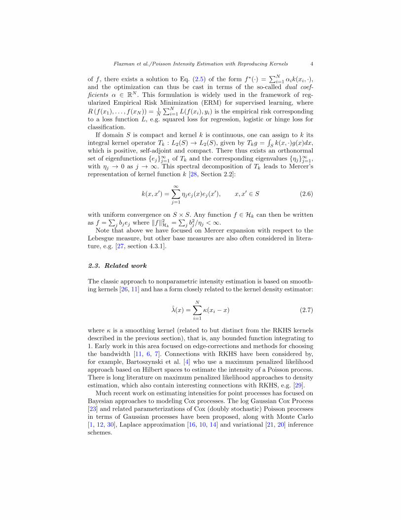
The classic approach to nonparametric intensity estimation is based on smooth-ing kernels [26, 11] and has a form closely related to the kernel density estimator:

λ(x) =

N∑i=1

κ(xi − x) (2.7)

where κ is a smoothing kernel (related to but distinct from the RKHS kernelsdescribed in the previous section), that is, any bounded function integrating to1. Early work in this area focused on edge-corrections and methods for choosingthe bandwidth [11, 6, 7]. Connections with RKHS have been considered by,for example, Bartoszynski et al. [4] who use a maximum penalized likelihoodapproach based on Hilbert spaces to estimate the intensity of a Poisson process.There is long literature on maximum penalized likelihood approaches to densityestimation, which also contain interesting connections with RKHS, e.g. [29].

Much recent work on estimating intensities for point processes has focused onBayesian approaches to modeling Cox processes. The log Gaussian Cox Process[23] and related parameterizations of Cox (doubly stochastic) Poisson processesin terms of Gaussian processes have been proposed, along with Monte Carlo[1, 12, 30], Laplace approximation [16, 10, 14] and variational [21, 20] inferenceschemes.


Another related body of literature concerns Cox processes with intensities pa-rameterized as the sum of squares of k Gaussian processes, called the permanentprocess [22]. Interestingly, calculating the density of the permanent process re-lies on a kernel transformation similar to the one we propose below. Unlike theseapproaches, however, we are not working in a doubly stochastic (Cox process)framework; rather we are taking a penalized maximum likelihood estimationperspective to estimate the intensity of an inhomogeneous Poisson process. Asfuture work, it would be worthwhile to explore deeper connections between ourformulation and the permanent process, e.g. by considering an RKHS formu-lation of Cox processes or by considering an inhomogeneous Poisson processwhose intensity is the sum of squares of functions in an RKHS.

3. Proposed method and kernel transformation

Let S be a compact domain of observations. Let k : S×S → R be a continuouspositive definite kernel, and Hk its corresponding RKHS of functions f : S → R.We model the intensity function λ(·) of an inhomogeneous Poisson process as:

λ(x) := af2(x), x ∈ S, (3.1)

which is parameterized by f ∈ Hk and an additional scale parameter a > 0.The flexibility of choosing k means that we can encode structural assumptionsof our domain, e.g. periodicity in time or periodic boundary conditions (seeSection 4.1.1). Note that we have squared f to ensure that the intensity is non-negative on S, a pragmatic choice that has previously appeared in the literature(e.g. [21]). While we lose identifiability (since f and −f are equivalent), as shownbelow we end up with a finite dimensional, and thus tractable, optimizationproblem.

The rationale for including a is that it allows us to decouple the overall scaleand units of the intensity (e.g. number of points per hour versus number ofpoints per year) from the penalty on the complexity of f which arises from theclassical regularized Empirical Risk Minimization framework (and which shoulddepend only on how complex, i.e. “wiggly” f is).

We use the inhomogeneous Poisson process likelihood from Eq. (2.4) towrite the log-likelihood of a Poisson process corresponding to the observationsx1, . . . , xN, for xi ∈ S, and intensity λ(·):

`(x1, . . . , xN |λ) =

N∑i=1

log(λ(xi))−∫S

λ(x)dx. (3.2)

We will consider the problem of minimization of the penalized negative loglikelihood, where the regularization term corresponds to the squared Hilbertspace norm of f in parametrization Eq. (3.1):

minf∈Hk

−

N∑i=1

log(af2(xi)) + a

∫S

f2(x)dx+ γ‖f‖2Hk

. (3.3)


This objective is akin to a classical regularized empirical risk minimizationframework over RKHS: there is a term that depends on evaluations of f atthe observed points x1, . . . , xN as well as a term corresponding to the RKHSnorm. However, the representer theorem does not apply directly to Eq. (3.3):since there is also a term given by the L2-norm of f , there is no guarantee thatthere is a solution of Eq. (3.3) that lies in spank(xi, ·)Ni=1. We will show thatEq. (3.3) fortunately still reduces to a finite-dimensional optimization problemcorresponding to a different kernel function k which we define below.

Using the Mercer expansion of k in Eq. (2.6), we can write the objectiveEq. (3.3) as follows:

J [f ] = −N∑i=1

log(af2(xi)) + a‖f‖2L2(S)+ γ‖f‖2Hk

(3.4)

= −N∑i=1

log(af2(xi)) + a

∞∑j=1

b2j + γ

∞∑j=1

b2jηj. (3.5)

The last two terms can now be merged together, giving

a

∞∑j=1

b2j + γ

∞∑j=1

b2jηj

=

∞∑j=1

b2jaηj + γ

ηj=

∞∑j=1

b2jηj(aηj + γ)−1

.

Now, if we define kernel k to be the kernel corresponding to the integral operatorTk := Tk(aTk + γI)−1, i.e., k is given by:

k(x, x′) =

∞∑j=1

ηjaηj + γ

ej(x)ej(x′), x, x′ ∈ S,

we see that:

J [f ] = −N∑i=1

log(af2(xi)) + ‖f‖2Hk. (3.6)

Thus, we have merged the two squared norm terms into a squared norm ina new RKHS. We note that a similar idea has previously been used to modifyGaussian process priors in [9], albeit in a different context, and that a similartransformation appears in the expression for the distribution of a permanentprocess [22]. We are now ready to state the representer theorem in terms ofkernel k.

Theorem 1. There exists a solution of Eq. (3.3) for observations x1, . . . , xN ,

which takes the form f∗(·) =∑Ni=1 αik(xi, ·).

Proof. Since∑j

b2jηj< ∞ if and only if

∑j

b2jηj(aηj+γ)−1 < ∞, i.e. f ∈ Hk ⇐⇒

f ∈ Hk, we have that the two spaces correspond to exactly the same set offunctions. Optimization over Hk is therefore equivalent to optimization overHk.


The proof now follows by applying the classical representer theorem in k tothe representation of the objective function in Eq. (3.6). We decompose f ∈ Hkas the sum of two functions:

f(·) =

N∑j=1

αj k(xj , ·) + v (3.7)

where v is orthogonal in Hk to the span of k(xj , ·)j . We prove that the first

term in the objective J [f ] given in Eq. (3.6),−∑Ni=1 log(af2(xi)), is independent

of v. It depends on f only through the evaluations f(xi) for all i. Using thereproducing property we have:

f(xi) = 〈f, k(xi, ·)〉Hk=∑j

αj k(xj , xi) + 〈v, k(xi, ·)〉Hk=∑j

αj k(xj , xi)

(3.8)where the last step is by orthogonality. Next we substitute into the regularizationterm:

γ‖∑j

αj k(xj , ·) + v‖2Hk= γ‖

∑j

αj k(xj , ·)‖2Hk+ ‖v‖2Hk

≥ γ‖∑j

αj k(xj , ·)‖2Hk.

(3.9)

Thus, the choice of v has no effect on the first term in J [f ] and a non-zero vcan only increase the second term ‖f‖2Hk

, so we conclude that v = 0 and that

f∗ =∑Nj=1 αj k(xj , ·) is the minimizer.

Remark 1. The notions of the inner product in Hk and Hk are different and

thus in general spank(xi, ·) 6= spank(xi, ·).Remark 2. Notice that unlike in a standard ERM setting, γ = 0 does not

recover the unpenalized risk, because γ appears in k. Notice further that theoverall scale parameter a also appears in k. This is important in practice, becauseit allows us to decouple the scale of the intensity (which is controlled by a) fromits complexity (which is controlled by γ).

Illustration. The eigenspectrum of k where k is a squared exponential kernelis shown in Figure 1 for various settings of a and γ. Reminiscent of spectralfiltering studied by Muandet, Sriperumbudur and Scholkopf [24], in the top plotwe see that depending on the settings of a and γ, eigenvalues of k are shrunkor inflated as compared to k(x, x′) which is shown in black. In the bottom plot,the values of k(0, x) are shown for the same set of kernels.

4. Computation of k

In this section, we consider first the case in which an explicit Mercer expansionis known, and then we consider the more commonly encountered situation inwhich we only have access to the parametric form of the kernel k(x, x′), so wemust approximate k. We show experimentally that our approximation is veryaccurate by considering the Sobolev kernel, which can be expressed in bothways.


2 4 6 8 10

0.0

0.2

0.4

0.6

0.8

rank

eige

nval

ue

k(t,t')a = 1, γ = 1 a = 2, γ = 1 a = 5, γ = 1 a = 1, γ = .1 a = 1, γ = .2 a = 1, γ = 5

0.0 0.1 0.2 0.3 0.4 0.5 0.6

01

23

4

t

valu

e of

ker

nel

k(t,t')a = 1, γ = 1 a = 2, γ = 1 a = 5, γ = 1 a = 1, γ = .1 a = 1, γ = .2 a = 1, γ = 5

Fig 1: Eigenspectrum of k (top) and values of k (bottom) for various settings ofa and γ.


4.1. Explicit Mercer Expansion

We start by assuming that we have a kernel k with an explicit Mercer expansionwith respect to a base measure of interest (usually the Lebesgue measure on S),so we have eigenvectors ej(x)j∈J and eigenvalues ηjj∈J :

k(x, x′) =∑j∈J

ηjej(x)ej(x′), (4.1)

with an at most countable index set J . Given a and γ we can calculate:

k(x, x′) =∑j∈J

ηjaηj + γ

ej(x)ej(x′) (4.2)

up to a desired precision as informed by the spectral decay in ηjj∈J . Belowwe consider kernels for which explicit Mercer expansions are known: a kernelon the Sobolev space [0, 1] with a periodic boundary condition, the squaredexponential kernel, and the Brownian bridge kernel. We also show how ourformulation can be extended to multiple dimensions using a tensor productformulation. Although not practical for large datasets, the Mercer expansionsgiven below, summing terms up to j = 50 (for which the error is less than10−5), can be used to evaluate approximations for the cases in which Mercerexpansions are not available.

4.1.1. Sobolev space on [0, 1] with a periodic boundary condition

We consider a kernel on the Sobolev space on [0, 1] with a periodic boundarycondition, proposed by Wahba [31, chapter 2] and recently used in Bach [2]. Thekernel is given by:

k(x, y) = 1 +

∞∑m=1

2 cos (2πm (x− y))

(2πm)2s

= 1 +

∞∑m=1

2

(2πm)2s[cos (2πmx) cos (2πmy) + sin (2πmx) sin (2πmy)] ,

= 1 +(−1)s−1

(2s)!B2s(x− y),

where s = 1, 2, . . . denotes the order of the Sobolev space and B2s(x − y) isthe Bernoulli polynomial of degree 2s applied to the fractional part of x−y. Thecorresponding RKHS is the space of functions on [0, 1] with absolutely contin-uous f, f ′, . . . , f (s−1) and square integrable f (s) satisfying a periodic boundarycondition f (l)(0) = f (l)(1), l = 0, . . . , s − 1. For more details, see [31, Chapter2].


Bernoulli polynomials admit a simple form for low degrees. In particular,

B2(t) = t2 − t+1

6,

B4(t) = t4 − 2t3 + t2 − 1

30,

B6(t) = t6 − 3t5 +5

2t4 − 1

2t2 +

1

42.

Moreover, note that:∫ 1

0

2 cos (2πmx) sin (2πm′x) dx = 0,∫ 1

0

2 cos (2πmx) cos (2πm′x) dx = δ(m−m′),∫ 1

0

2 sin (2πmx) sin (2πm′x) dx = δ(m−m′).

Thus, the desired Mercer expansion (with respect to the Lebesgue measure) isgiven by k(x, y) =

∑m∈Z ηmem(x)em(y) with eigenfunctions e0(x) = 1 and for

m = 1, 2, . . ., em(x) =√

2 cos (2πmx), e−m(x) =√

2 sin (2πmx) and corre-sponding eigenvalues η0 = 1, ηm = η−m = (2πm)−2s.

Now, the adjusted kernel k(x, y) from (4.2) is given by

k(x, y) =∑m∈Z

ηmηm + γ

em(x)em(y)

=1

1 + γ+

∞∑m=1

2 cos (2πm (x− y))

1 + γ(2πm)2s.

4.1.2. Squared exponential kernel

A Mercer expansion for the squared exponential kernel was proposed in [35]and refined in [13]. However, this expansion is with respect to a Gaussian mea-sure on R, i.e., it consists of eigenfunctions which form an orthonormal set inL2(R, ν) where ν = N (0, `2I). The formalism can therefore be used to esti-mate Poisson intensity functions with respect to such Gaussian measure. In theclassical framework, where the intensity is with respect to a Lebesgue measure,numerical approximations of Mercer expansion, as described in Section 4.2 areneeded. Following the exposition in [27, section 4.3.1] and the relevant errata1

we parameterize the kernel as:

k(x, x′) = exp(−‖x− x′‖2

2σ2) (4.3)

1http://www.gaussianprocess.org/gpml/errata.html


The Mercer expansion with respect to ν = N (0, `2I) then has the eigenvalues

ηi =

√2a

ABi, (4.4)

and eigenfunctions

ei(x) =1√√a/c 2ii!

exp(−(c− a)x2)Hi(√

2cx) (4.5)

where Hi is the i-th order (physicist’s) Hermite polynomial, a = 14σ2 , b = 1

2`2 ,

c =√a2 + 2ab, A = a + b + c, and B = b/A. Thus we have the following

eigenvalues for k:

ηi =ηi

aηi + γ=

1

a+ γ√

A2aB

−i(4.6)

while the eigenfunctions remain the same.

4.1.3. Brownian Bridge kernel

This is the kernel on [0, 1], given by

k(x, y) = min(x, y)− xy =

∞∑m=1

2 sin(πmx) sin(πmy)

π2m2,

with the eigenvalues and eigenfunctions in the Mercer expansion with respectto Lebesgue measure

ηm =1

π2m2, em(x) =

√2 sin (πmx) , m = 1, 2, . . . . (4.7)

Thus one can form

k(x, y) =∞∑m=1

ηmηm + c

em(x)em(y)

=

∞∑m=1

2 sin(πmx) sin(πmy)

1 + cπ2m2.

The functions in the corresponding RKHS are pinned to zero at both endsof the segment.

4.1.4. Extending the Mercer expansion to multiple dimensions

The extension of any kernel to higher dimensions can be constructed by con-sidering tensor product spaces: Hk1⊗k2 (where k1 and k2 could potentially be


different kernels with different hyperparameters). If k1 has eigenvalues ηi andeigenfunctions ei and k2 has eigenvalues δj and eigenfunctions fj , then the eigen-values of the product space are then given by the Cartesian product ηiδj ,∀i, j,and similarly the eigenfunctions are given by ei(x)fj(y). Our regularized kernelhas the following Mercer expansion:

k1 ⊗ k2((x, y), (x′, y′)) =∑ij

ηiδjaηiδj + γ

ei(x)ei(x′)fj(y)fj(y

′) (4.8)

Notice that k1 ⊗ k2 is the kernel corresponding to the integral operator (Tk1 ⊗Tk2)(aTk1 ⊗ Tk2 + γI)−1 which is different than k1 ⊗ k2.

Notice that this approach does not lead to a method that scales well in highdimensions, which is further motivation for the approximations developed below.

4.2. Numerical approximation when Mercer expansions are notavailable

We propose an approximation to k given access only to a kernel k for which wedo not have an explicit Mercer expansion with respect to Lebesgue measure. Weonly assume that we can form Gram matrices corresponding to k and calculatetheir eigenvectors and eigenvalues. As a side benefit, this representation will alsoenable scalable computations through Toeplitz / Kronecker algebra [10, 15, 14]or primal reduced rank approximations [33].

Let us first consider the one-dimensional case and construct a uniform gridu = (u1, . . . , um) on [0, 1]. Then the integral kernel operator Tk can be approx-imated with the (scaled) kernel matrix 1

mKuu : Rm → Rm, where [Kuu]ij =

k(ui, uj), and thus Kuu is approximately Kuu

(amKuu + γI

)−1. Note that for

the general case of multidimensional domains S, the kernel matrix would haveto be multiplied by vol(S). Without loss of generality we assume vol(S) = 1below.

We are not primarily interested in evaluations of k on this grid, but on theobservations x1, . . . , xN . Simply adding the observations into the kernel matrixis not an option however, as it changes the base measure with respect to whichthe integral kernel operator is to be computed (Lebesgue measure on [0, T ]).Thus, we consider the relationship between the eigendecomposition of Kuu andthe eigenvalues and eigenfunctions of the integral kernel operator Tk.

Let λui , eui be the eigenvalue/eigenvector pairs of the matrix Kuu, i.e., its

eigendecomposition is given by Kuu = QΛQ> =∑mi=1 λ

ui eui (eui )>. Then the

estimates of the eigenvalues/eigenfunctions of the integral operator Tk are givenby the Nystrom method (see Rasmussen and Williams [27, Section 4.3] andreferences therein, especially Baker [3]):

ηi =1

mλui , ei(x) =

√m

λuiKxueui , (4.9)


with Kxu = [k(x, u1), . . . , k(x, um)], leading to:k(x, x′) =

m∑i=1

ηiaηi + γ

ei(x)ei(x′) (4.10)

=

m∑i=1

1mλ

ui

amλ

ui + γ

· m

(λui )2Kxueui (eui )>Kux′

= Kxu

m∑i=1

1(amλ

ui + γ

)λui

eui (eui )>

Kux′ .

For an estimate of the whole matrix Kxx we thus haveKxx = Kxu

m∑i=1

1(amλ

ui + γ

)λui

eui (eui )>

Kux

= KxuQ( am

Λ2 + γΛ)−1

Q>Kux. (4.11)

The above is reminiscent of the Nystrom method [33] proposed for speedingup Gaussian process regression. It has computational cost O(m3 + N2m). Areduced rank representation for Eq. (4.11) is straightforward by considering onlythe top p eigenvalues/eigenvectors of Kuu. Furthermore, a primal representationwith the features corresponding to kernel k is readily available and is given by

φ(x) =( am

Λ2 + γΛ)−1/2

Q>Kux, (4.12)

which allows linear computational cost in the number N of observations.For D > 1 dimensions, one can exploit Kronecker and Toeplitz algebra ap-

proaches. Assuming that the Kuu matrix corresponds to a Cartesian prod-uct structure of the one-dimensional grids of size m, one can write Kuu =K1 ⊗ K2 · · · ⊗ KD. Thus, the eigenspectrum can be efficiently calculated byeigendecomposing each of the smaller m × m matrices K1, . . . ,KD and thenapplying standard Kronecker algebra, thereby avoiding ever having to form theprohibitively large mD ×mD matrix Kuu. For regular grids and stationary ker-nels, each small matrix will be Toeplitz structured, yielding further efficiencygains [34]. The resulting approach thus scales linearly in dimension D.

An even simpler alternative to the above is to sample the points u1, . . . , umuniformly from the domain S using Monte Carlo or Quasi-Monte Carlo (see [25]for a discussion in the context of RKHS). We found this approach to work wellin practice in high-dimensions (D = 15), even when m was fixed, meaning thatthe scaling was effectively independent of the dimension D.

Using the Sobolev kernel in Sec. 4.1.1, we compared the exact calculation ofKuu with s = 1, a = 10, and γ = .5 to our approximate calculation. For illus-tration we compared a coarse grid of size 10 on the unit interval (left) to a finergrid of size 100. The RMSE was 2E-3 for the coarse grid and 1.6E-5 for the finegrid, as shown in Fig. 2. In the same figure we compared the exact calculationof Kxx with s = 1, a = 10, and γ = .5 to our Nystrom-based approximation,where x1, . . . , x400 ∼ Beta(.5, .5) distribution. The RMSE was 0.98E-3. A low-rank approximation using only the top 5 eigenvalues gives the RMSE of 1.6E-2.


As Figure 2, demonstrates, good approximation is possible with a fairly coarsegrid u = (u1, . . . , um) as well as with a low-rank approximation.

0.2 0.4 0.6 0.8

0.05

0.10

0.15

0.20

(a)

kern

el v

alue

0.0 0.2 0.4 0.6 0.8 1.0

0.05

0.10

0.15

0.20

(b)

kern

el v

alue

0.0 0.2 0.4 0.6 0.8 1.0

0.05

0.10

0.15

0.20

(c)

kern

el v

alue

0.0 0.2 0.4 0.6 0.8 1.0

0.05

0.10

0.15

0.20

(d)

kern

el v

alue

Fig 2: Using the Sobolev kernel in Sec. 4.1.1, we compared the exact calcu-lation of Kuu with s = 1, a = 10, and γ = .5 to our approximate calcula-tion. For illustration we tried a coarse grid of size 10 on the unit interval (topleft) to a finer grid of size 100 (top right). The RMSE was 2E-3 for the coarsegrid and 1.6E-5 for the fine grid. We compare the exact calculation of Kxx

with s = 1, a = 10, and γ = .5 to our Nystrom-based approximation, wherex1, . . . , x400 ∼ Beta(.5, .5) distribution (bottom left). The RMSE was 0.98E-3.A low-rank approximation using only the top 5 eigenvalues gives the RMSE of1.6E-2 (bottom right).

5. Inference

The penalized risk can be readily minimized with gradient descent.2 Let α =[α1, . . . , αN ]> and K be the Gram matrix corresponding to k such that Kij =

k(xi, xj). Then [f(x1), . . . , f(xN )]> = Kα and the gradient of the objective

2While the objective is not convex, in practice we observed very fast convergence, andstable results given random starting points.


function J from (3.6) is given by

∇αJ = −∇α∑i

log(af2(xi)) + γ∇α‖f‖2Hk

= −∇α∑i

log(a(∑j

kijαj)2) + γ∇αα>Kα

= −∑i

2a(∑j kijαj)∇α

∑j kijαj

a(∑j kijαj)

2+ 2γKα

= −∑i

2K·i∑j kijαj

+ 2γKα

= −2∑i

(K·i./(Kα)) + 2γKα

where ./ denotes element-wise division. Computing K requires O(N2) time andmemory, and each gradient and likelihood computation requires matrix-vectormultiplications which are also O(N2). Overall, the running time is O(qN2) forq iterations of the gradient descent method, where q is usually very small inpractice.

5.1. Hyperparameter selection

Analogously to the classical problem of bandwidth selection in kernel intensityestimation (e.g. [11, 6, 7]), some criteria must be adopted in order to selecthyperparameters of the kernel k and also γ and a. We suggest crossvalidating onthe negative log-likelihood of the inhomogeneous Poisson process (i.e. before weintroduced the penalty term) from Eq. (3.2). The difficulty with this approach isthat we must deal with the integral

∫Sf2(u)du of the intensity over the domain,

which, for our model f(·) =∑Nj=1 αj k(xj , ·) is generally intractable. As an

approximation, we suggest either grid or Monte Carlo integration. Recall thatin Section 4.2 we approximated k using a set of locations u = (u1, . . . , um). Wecan reuse these points to approximate the integral:∫

S

f2(u)du ≈ 1

m

∑i

f2(ui). (5.1)

As f(ui) = Kuixα, this approximation is given by 1mα>KxuKuxα.

6. Naıve RKHS model

In this section, we compare the proposed approach, which uses the represen-ter theorem in the transformed kernel k, to the naıve one, where a solution toEq. (3.3) of the form f(·) =

∑Nj=1 αjk(xj , ·) is sought even though the repre-

senter theorem in k need not hold. Despite being theoretically suboptimal, thisis a natural model to consider, and it might perform well in practice.


The corresponding optimization problem is:

minf∈Hk

−

N∑i=1

log(af2(xi)) + a

∫S

f2(x)dx+ γ‖f‖2Hk

While the first and the last term are straightforward to calculate for any

f(·) =∑j αjk(xj , ·),

∫Sf2(x)dx needs to be estimated. As in the previous

section, we consider a uniform grid or set of sampled points u = (u1, . . . , um)covering the domain and use approximation∫

S

f2(u)du ≈ 1

m

∑i

f2(ui) =1

nα>KxuKuxα. (6.1)

The optimization problem thus reads:

minα∈RN

−

N∑i=1

log(a(α>Kxxi)2) + α>

(anKxuKux + γKxx

)α

. (6.2)

As above, the gradient of this objective with respect to α can be readily calcu-lated, and optimized with gradient descent.

7. Experiments

We use cross-validation to choose the hyperparameters in our methods: a, thefixed intensity, γ, the roughness penalty, and the length-scale of the kernel k,minimizing the negative log-likelihood as described in Section 5.1.

To calculate RMSE, we either make predictions at a grid of locations andcalculate RMSE compared to the true intensity at that grid or for the high-dimensional synthetic example we pick a new uniform sample of locations overthe domain and calculate the RMSE at these locations. We used limited memoryBFGS in all experiments involving optimization, and found that it convergedvery quickly and was not sensitive to initial values. Code for our experiments isavailable at https://github.com/BigBayes/kernelpoisson.

7.1. 1-d synthetic Example

We generated a synthetic intensity using the Mercer expansion of a SE kernelwith lengthscale 0.5, producing a random linear combination of 64 basis func-tions, weighted with iid draws α ∼ N (0, 1). In Fig. 3 we compare ground truthto estimates made with: our RKHS method with SE kernel, the naıve RKHSapproach with SE kernel, and classical kernel intensity estimation with band-width selected by crossvalidation. The results are typical of what we observedon 1D and 2D examples: given similar kernel choices, each method performedsimilarly, and numerically there was not a significant difference in terms of theRMSE compared to the true underlying intensity.

https://github.com/BigBayes/kernelpoisson


0.0 0.2 0.4 0.6 0.8 1.0

010

020

030

040

050

060

0

x

inte

nsity

truekernel smoothedRKHSRKHS (naive)

Fig 3: A synthetic dataset, comparing our RKHS method,the naıve model, and kernel smoothing to a synthetic in-tensity “true”. The rug plot at bottom gives the locationof points in the realized point pattern. The RMSE for eachmethod was similar.

7.2. Environmental datasets

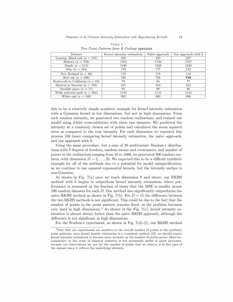
Next we demonstrate our method on a collection of two-dimensional environ-mental datasets giving the locations of trees. Intensity estimation is a standardfirst step in both exploratory analysis and modelling of these types of datasets,which were obtained from the R package spatstat. We calculated the intensityusing various approaches: our proposed RKHS method with k with a squared ex-ponential kernel, the naıve RKHS method with squared exponential kernel, andclassical kernel intensity estimation (KIE) with edge correction. Each methodused a squared exponential kernel. We report average held-out cross-validatedlikelihoods in Table 1. With the exception of our method performing better onthe Red oak dataset, each method had comparable performance. It is interestingto note, however, that our method does not require any explicit edge correction3,because we are optimizing a likelihood which explicitly takes into account thewindow. A plot of the resulting intensity surfaces for each method and the effectof edge correction are shown in Fig. 4 for the Black oak dataset.

3Because no points are observed outside the window S, intensity estimates near the edgeare biased downwards [17].


(a) KIE with edge correction (b) KIE without edge correction

(c) Our RKHS method with k (d) Naıve RKHS method

Fig 4: Location of white oak trees in Lansing, Michigan, smoothed with various ap-proaches. Squared exponential kernels are used throughout. Edge correction makes anoticeable difference for classical kernel intensity estimation. Comparing (a) and (c) itis clear that our method is automatically performing edge correction.

7.3. High dimensional synthetic examples

We generated random intensity surfaces in the unit hypercube for dimensionsD = 2, . . . , 15. The intensity was given by a constant multiplied by the square ofthe sum of 20 multivariate Gaussian pdfs with random means and covariances.The constant was automatically adjusted so that the number of points in therealizations would be held close to constant, in the range 190-210. We expected


Table 1

Tree Point Patterns from R Package spatstat

Dataset Kernel intensity estimation Naıve approach Our approach with kLansing: Black oak (n = 135) 234 233 227

Hickory (n = 703) 1763 1746 1757Maple (n = 514) 1239 1228 1233Misc (n = 105) 179 177 172

New Zealand (n = 86) 119 119 119Red oak (n = 346) 726 726 739

Redwoods in California (n = 62) 79 84 77Spruces in Saxonia (n = 134) 215 212 212

Swedish pines (n = 71) 91 89 90Waka national park (n = 504) 1142 1141 1144

White oak (n = 448) 992 992 996

this to be a relatively simple synthetic example for kernel intensity estimationwith a Gaussian kernel in low dimensions, but not in high dimensions. Fromeach random intensity, we generated two random realizations, and trained ourmodel using 2-fold crossvalidation with these two datasets. We predicted theintensity at a randomly chosen set of points and calculated the mean squarederror as compared to the true intensity. For each dimension we repeated thisprocess 100 times comparing kernel intensity estimation, the naıve approach,and our approach with k.

Using the same procedure, but a sum of 20 multivariate Student-t distribu-tions with 5 degrees of freedom, random means and covariances, and number ofpoints in the realizations ranging from 10 to 1000, we generated 500 random sur-faces, with dimension D = 2, . . . , 25. We expected this to be a difficult syntheticexample for all of the methods due to a potential for model misspecification,as we continue to use squared exponential kernels, but the intensity surface isnon-Gaussian.

As shown in Fig. 7(a) once we reach dimension 9 and above, our RKHSmethod with k begins to outperform kernel intensity estimation, where per-formance is measured as the fraction of times that the MSE is smaller across100 random datasets for each D. Our method also significantly outperforms thenaıve RKHS method as shown in Fig. 7(b). For D = 15 the difference betweenthe two RKHS methods is not significant. This could be due to the fact that thenumber of points in the point pattern remains fixed, so the problem becomesvery hard in high dimensions.4 As shown in the Fig. 7(c), kernel intensity es-timation is almost always better than the naıve RKHS approach, although thedifference is not significant in high dimensions.

For the Student-t experiment, as shown in Fig. 7(d)-(f), our RKHS method

4Note that our experiments are sensitive to the overall number of points in the syntheticpoint patterns; since kernel density estimation is a consistent method [32], we should expectkernel intensity estimation to become more accurate as the number of points grows. However,consistency in the sense of classical statistics is not necessarily useful in point processes,because our observations are not iid; the number of points that we observe is in fact part ofthe dataset since it reflects the underlying intensity.


always outperforms kernel intensity estimation and is better than the naıvemethod in dimensions below D = 20. To assess the amount of improvement,rather than just its statistical significance, we compared the percent improve-ment in terms of MSE gained by our method versus the competitors, just fo-cusing on D = 10 in Fig. 8. On this metric (intuitively, “how much do youexpect to improve on average”) our method shows reasonably stable results ascompared to KIE, while the performance of the naıve method is revealed tobe very variable. Indeed, the standard deviation across the random surfaces forD = 10 of the MSE was 56 for both our method and KDE but 166 for the naıvemethod, perhaps due to overfitting.

7.4. Computational complexity

Using the synthetic data experimental setup, we evaluated the time complexityof our method with respect to dimensionality d, number of points in the pointpattern dataset n, and number of points s used to estimate k (Fig. 6), confirmingour theoretical analysis.

The effect of the dimensionality d was negligible in practice, because the maincalculations rely only on an n × n Gram matrix whose calculation is relativelyfast even for high dimensions. Our method’s time complexity scales as O(n2)as shown in Fig. 5 (but as discussed in Section 4.2, a primal representation isavailable which would give linear scaling.) where we used s = 200 sample pointsto estimate k. While a small s worked well in practice, we investigated muchlarger values of s. As shown in Fig. 6 the time complexity scaled as O(s2) wherethe number of points was fixed to be 150; note that we fixed the rank of theeigendecomposition to be 20.

1000 2000 3000 4000

5015

025

035

0

number of points in dataset

runt

ime

in s

econ

ds

Fig 5: Run-time of our method versus number of points in the point patterndataset.


1000 2000 3000 4000 5000

1030

50

number of sample locations for calculating kernel

runt

ime

in s

econ

ds

Fig 6: Run-time of our method versus number of sample points used to calculatek.

7.5. Spatiotemporal point pattern of crimes

To demonstrate the ability to use domain specific kernels and learn interpretablehyperparameters, we used 12 weeks (84 days) of geocoded, date-stamped reportsof theft obtained from Chicago’s data portal (data.cityofchicago.org) startingJanuary 1, 2004, a relatively large spatiotemporal point pattern consisting of18,441 events. We used the following kernel: exp(−.5s2/λ2s)(exp(−2 sin2(tπp))+1)(exp(−.5t2/λ2t )) which is the product of a separable squared exponential spaceand decaying periodic time kernel (with frequency p in a time domain normal-ized to range from 0 to 1) plus a separable squared exponential space and timekernel. After finding reasonable values for the lengthscales and other hyperpa-rameters of k through exploratory data analysis, we used 2-fold cross-validationand calculated average test log-likelihoods for the number of total cycles p in the84 weeks = 1, 2, . . . , 14 or equivalently a period of length 12 weeks (meaning nocycle), 6 weeks, ..., 6 days. These log-likelihoods are shown in Fig. 9; we foundthat the most likely frequency is 12, or equivalently a period lasting 1 week.This makes sense given known day-of-week effects on crime.

8. Conclusion

We presented a novel approach to inhomogeneous Poisson process intensity esti-mation using a representer theorem formulation in an appropriately transformedRKHS, providing a scalable approach giving strong performance on syntheticand real-world datasets. Our approach outperformed the classical baseline ofkernel intensity estimation and a naıve approach for which the representer the-orem guarantees did not hold. In future work, we will consider marked Poisson


(a)

Dimension

% o

f tim

e R

KH

S o

utpe

rfor

ms

KIE

2 3 5 7 9 11 13 15

025

5075

100

(b)

Dimension

% o

f tim

e R

KH

S o

utpe

rfor

ms

naiv

e

2 3 5 7 9 11 13 15

025

5075

100

(c)

Dimension

% o

f tim

e K

IE o

utpe

rfor

ms

naiv

e

2 3 5 7 9 11 13 15

025

5075

100

(d)

Dimension

% o

f tim

e R

KH

S o

utpe

rfor

ms

KIE

5 7 9 11 13 15 17 19 21 23 25

025

5075

100

(e)

Dimension% o

f tim

e R

KH

S o

utpe

rfor

ms

naiv

e

5 7 9 11 13 15 17 19 21 23 25

025

5075

100

(f)

Dimension

% o

f tim

e K

IE o

utpe

rfor

ms

naiv

e

5 7 9 11 13 15 17 19 21 23 25

025

5075

100

Fig 7: Three methods were compared: our RKHS method, the naıve RKHSmethod, and kernel intensity estimation, based on 100 random surfaces for eachdimension D in two experimental setups. In (a)-(c), the intensity surface wasthe squared sum of skewed multivariate Gaussians. In (d)-(f) the surface was amixture of skewed multivariate Student-t distributions, with 5 degrees of free-dom. In (a) and (d): comparison of our RKHS method versus KIE. In (b) and(e): our RKHS method versus the naıve RKHS method. In (c) and (f): compari-son of KIE and the naıve RKHS approach. We used squared exponential kernelsfor all methods. In the Gaussian case (a)-(c), our method significantly outper-forms kernel intensity estimation as the dimension increases, and outperformsthe naıve method throughout. Kernel intensity estimation almost always out-performs the naıve approach. In the Student-t case (d)-(f), our method alwaysoutperforms kernel intensity estimation, and outperforms the naıve approachuntil very high dimensions. Neither kernel intensity estimation nor the naıveapproach are consistently better than each other.


processes and other more complex point process models, as well as Bayesianextensions akin to Cox process modeling.

References

[1] Adams, R. P., Murray, I. and MacKay, D. J. (2009). Tractable non-parametric Bayesian inference in Poisson processes with Gaussian processintensities. In Proceedings of the 26th Annual International Conference onMachine Learning 9–16. ACM.

[2] Bach, F. (2015). On the Equivalence between Quadrature Rules and Ran-dom Features. arXiv:1502.06800.

[3] Baker, C. T. H. (1977). The Numerical Treatment of Integral Equations.Monographs on Numerical Analysis Series. Oxford : Clarendon Press.

[4] Bartoszynski, R., Brown, B. W., McBride, C. M. and Thomp-son, J. R. (1981). Some nonparametric techniques for estimating the inten-sity function of a cancer related nonstationary Poisson process. The Annalsof Statistics 1050–1060.

[5] Berlinet, A. and Thomas-Agnan, C. (2004). Reproducing KernelHilbert Spaces in Probability and Statistics. Kluwer.

[6] Berman, M. and Diggle, P. (1989). Estimating weighted integrals ofthe second-order intensity of a spatial point process. Journal of the RoyalStatistical Society. Series B (Methodological) 81–92.

[7] Brooks, M. M. and Marron, J. S. (1991). Asymptotic optimality of theleast-squares cross-validation bandwidth for kernel estimates of intensityfunctions. Stochastic Processes and their Applications 38 157–165.

[8] Cressie, N. and Wikle, C. K. (2011). Statistics for spatio-temporal data465. Wiley.

[9] Csato, L., Opper, M. and Winther, O. (2001). TAP Gibbs Free En-ergy, Belief Propagation and Sparsity. In Advances in Neural InformationProcessing Systems 657–663.

[10] Cunningham, J. P., Shenoy, K. V. and Sahani, M. (2008). Fast Gaus-sian process methods for point process intensity estimation. In ICML 192–199. ACM.

[11] Diggle, P. (1985). A kernel method for smoothing point process data.Applied Statistics 138–147.

[12] Diggle, P. J., Moraga, P., Rowlingson, B., Taylor, B. M. et al.(2013). Spatial and spatio-temporal Log-Gaussian Cox processes: extendingthe geostatistical paradigm. Statistical Science 28 542–563.

[13] Fasshauer, G. E. and McCourt, M. J. (2012). Stable evaluation ofGaussian radial basis function interpolants. SIAM Journal on ScientificComputing 34 A737–A762.

[14] Flaxman, S. R., Wilson, A. G., Neill, D. B., Nickisch, H. andSmola, A. J. (2015). Fast Kronecker inference in Gaussian processes withnon-Gaussian likelihoods. International Conference on Machine Learning.


[15] Gilboa, E., Saatci, Y. and Cunningham, J. (2013). Scaling Multidi-mensional Inference for Structured Gaussian Processes. Pattern Analysisand Machine Intelligence, IEEE Transactions on PP 1-1.

[16] Illian, J. B., Sørbye, S. H., Rue, H. et al. (2012). A toolbox for fit-ting complex spatial point process models using integrated nested Laplaceapproximation (INLA). The Annals of Applied Statistics 6 1499–1530.

[17] Jones, M. C. (1993). Simple boundary correction for kernel density esti-mation. Statistics and Computing 3 135–146.

[18] Kimeldorf, G. and Wahba, G. (1971). Some results on Tchebycheffianspline functions. Journal of Mathematical Analysis and Applications 33 82- 95.

[19] Kingman, J. F. C. (1993). Poisson processes. Oxford Studies in Probability3. The Clarendon Press Oxford University Press, New York. Oxford SciencePublications. MR1207584 (94a:60052)

[20] Kom Samo, Y. L. and Roberts, S. (2015). Scalable NonparametricBayesian Inference on Point Processes with Gaussian Processes. In ICML2227–2236.

[21] Lloyd, C., Gunter, T., Osborne, M. and Roberts, S. (2015). Vari-ational Inference for Gaussian Process Modulated Poisson Processes. InICML 1814–1822.

[22] McCullagh, P. and Møller, J. (2006). The permanental process. Ad-vances in applied probability 873–888.

[23] Møller, J., Syversveen, A. R. and Waagepetersen, R. P. (1998).Log Gaussian Cox processes. Scandinavian Journal of Statistics 25 451–482.

[24] Muandet, K., Sriperumbudur, B. and Scholkopf, B. (2014). KernelMean Estimation via Spectral Filtering. In Advances in Neural InformationProcessing Systems.

[25] Oates, C. J. and Girolami, M. A. (2016). Control Functionals for Quasi-Monte Carlo Integration. In Proceedings of the 19th International Confer-ence on Artificial Intelligence and Statistics, AISTATS 2016, Cadiz, Spain,May 9-11, 2016 (A. Gretton and C. C. Robert, eds.). JMLR Workshopand Conference Proceedings 51 56–65. JMLR.org.

[26] Ramlau-Hansen, H. (1983). Smoothing Counting Process Intensities byMeans of Kernel Functions. Ann. Statist. 11 453–466.

[27] Rasmussen, C. E. and Williams, C. K. (2006). Gaussian processes formachine learning. MIT Press.

[28] Scholkopf, B. and Smola, A. J. (2002). Learning with kernels: supportvector machines, regularization, optimization and beyond. MIT Press.

[29] Silverman, B. W. (1982). On the Estimation of a Probability DensityFunction by the Maximum Penalized Likelihood Method. Ann. Statist. 10795–810.

[30] Teh, Y. W. and Rao, V. (2011). Gaussian process modulated renewalprocesses. In Advances in Neural Information Processing Systems 2474–2482.

[31] Wahba, G. (1990). Spline models for observational data 59. Siam.

http://www.ams.org/mathscinet-getitem?mr=MR1207584


[32] Wied, D. and Weißbach, R. (2012). Consistency of the kernel densityestimator: a survey. Statistical Papers 53 1–21.

[33] Williams, C. and Seeger, M. (2001). Using the Nystrom method tospeed up kernel machines. In Advances in Neural Information ProcessingSystems 682–688.

[34] Wilson, A. G., Dann, C. and Nickisch, H. (2015). Thoughts on Mas-sively Scalable Gaussian Processes. arXiv:1511.01870.

[35] Zhu, H., Williams, C. K., Rohwer, R. and Morciniec, M. (1997).Gaussian regression and optimal finite dimensional linear models. Technicalreport.


(a)

% improvement of RKHS over KIE

Fre

quen

cy

0 20 40 60 80

010

020

030

0

(b)

% improvement of RKHS over naive

Fre

quen

cy

0 20 40 60 80

050

100

150

Fig 8: To understand the practical (as opposed to statistical) significance of theresults in Fig. 7(d)-(f), where we generated random surfaces by squaring thesums of multivariate Student-t distributions, we considered dimension D = 10,in which our RKHS method was better than both the naıve method and kernelintensity estimation (KIE) but there was not a significant difference betweenKIE and the naıve method, and calculated the percent improvement in terms ofMSE comparing our RKHS method to the naıve method (left) and our RKHSmethod to and kernel intensity estimation (KIE) (right). The improvement ofour method over KIE is apparent, albeit perhaps only modest in this example.Meanwhile, our method is sometimes quite a bit better than the naıve method,which is often very inaccurate.


4000

050

000

6000

0

frequency

log−

likel

ihoo

d

1 2 4 6 8 10 12 14

Fig 9: Log-likelihood for various frequencies of a periodic spatiotemporal kernel in adataset of 18,441 geocoded, date-stamped theft events from Chicago, using our RKHSmodel. The dataset is for 12 weeks starting January 1, 2004, and the maximum log-likelihood is attained when the frequency is 12, meaning that there is a weekly cycle inthe data. Results using the naıve model were less sensible, with a maximum at period1 (indicating no periodicity), with periods 5 and 2 (corresponding to a 16.8 day cycleand a 42 day cycle) also having high likelihoods.

poisson intensity estimation with reproducing kernels · poisson intensity estimation with ......

Documents