Poisson–Gamma Dynamical Systems

Aaron ScheinCollege of Information and Computer Sciences

University of Massachusetts AmherstAmherst, MA 01003

aschein@cs.umass.edu

Mingyuan ZhouMcCombs School of Business

The University of Texas at AustinAustin, TX 78712

mingyuan.zhou@mccombs.utexas.edu

Hanna WallachMicrosoft Research New York641 Avenue of the Americas

New York, NY 10011hanna@dirichlet.net

Abstract

We introduce a new dynamical system for sequentially observed multivariate countdata. This model is based on the gamma–Poisson construction—a natural choice forcount data—and relies on a novel Bayesian nonparametric prior that ties and shrinksthe model parameters, thus avoiding overfitting. We present an efficient MCMC in-ference algorithm that advances recent work on augmentation schemes for inferencein negative binomial models. Finally, we demonstrate the model’s inductive biasusing a variety of real-world data sets, showing that it exhibits superior predictiveperformance over other models and infers highly interpretable latent structure.

1 Introduction

Sequentially observed count vectors y(1), . . . ,y(T ) are the main object of study in many real-worldapplications, including text analysis, social network analysis, and recommender systems. Count datapose unique statistical and computational challenges when they are high-dimensional, sparse, andoverdispersed, as is often the case in real-world applications. For example, when tracking counts ofuser interactions in a social network, only a tiny fraction of possible edges are ever active, exhibitingbursty periods of activity when they are. Models of such data should exploit this sparsity in order toscale to high dimensions and be robust to overdispersed temporal patterns. In addition to these charac-teristics, sequentially observed multivariate count data often exhibit complex dependencies within andacross time steps. For example, scientific papers about one topic may encourage researchers to writepapers about another related topic in the following year. Models of such data should therefore capturethe topic structure of individual documents as well as the excitatory relationships between topics.

The linear dynamical system (LDS) is a widely used model for sequentially observed data, withmany well-developed inference techniques based on the Kalman filter [1, 2]. The LDS assumesthat each sequentially observed V -dimensional vector r(t) is real valued and Gaussian distributed:r(t) ∼ N (Φθ(t),Σ), where θ(t) ∈ RK is a latent state, with K components, that is linked to theobserved space via Φ ∈ RV×K . The LDS derives its expressive power from the way it assumesthat the latent states evolve: θ(t) ∼ N (Πθ(t−1),∆), where Π ∈ RK×K is a transition matrix thatcaptures between-component dependencies across time steps. Although the LDS can be linked tonon-real observations via the extended Kalman filter [3], it cannot efficiently model real-world countdata because inference isO((K+V )3) and thus scales poorly with the dimensionality of the data [2].

30th Conference on Neural Information Processing Systems (NIPS 2016), Barcelona, Spain.

Many previous approaches to modeling sequentially observed count data rely on the generalizedlinear modeling framework [4] to link the observations to a latent Gaussian space—e.g., via thePoisson–lognormal link [5]. Researchers have used this construction to factorize sequentially ob-served count matrices under a Poisson likelihood, while modeling the temporal structure usingwell-studied Gaussian techniques [6, 7]. Most of these previous approaches assume a simple Gaus-sian state-space model—i.e., θ(t) ∼ N (θ(t−1),∆)—that lacks the expressive transition structureof the LDS; one notable exception is the Poisson linear dynamical system [8]. In practice, theseapproaches exhibit prohibitive computational complexity in high dimensions, and the Gaussianassumption may fail to accommodate the burstiness often inherent to real-world count data [9].

1988 1991 1994 1997 20005

10

15

20

25

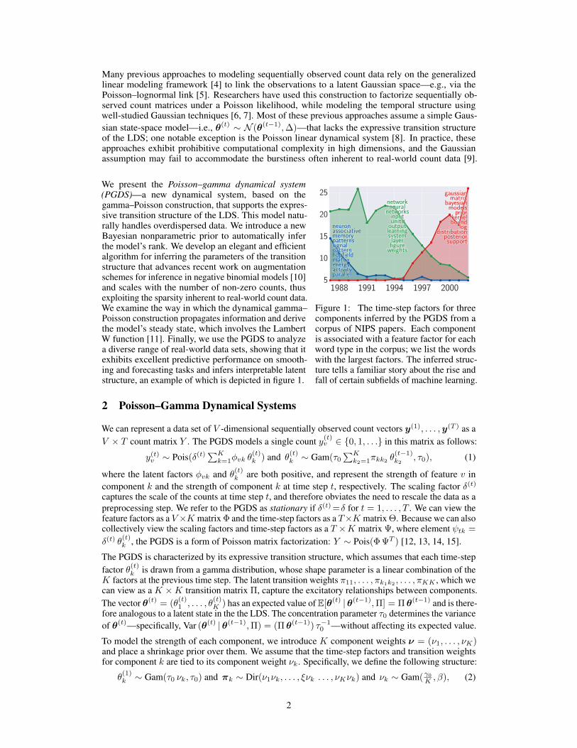
Figure 1: The time-step factors for threecomponents inferred by the PGDS from acorpus of NIPS papers. Each componentis associated with a feature factor for eachword type in the corpus; we list the wordswith the largest factors. The inferred struc-ture tells a familiar story about the rise andfall of certain subfields of machine learning.

We present the Poisson–gamma dynamical system(PGDS)—a new dynamical system, based on thegamma–Poisson construction, that supports the expres-sive transition structure of the LDS. This model natu-rally handles overdispersed data. We introduce a newBayesian nonparametric prior to automatically inferthe model’s rank. We develop an elegant and efficientalgorithm for inferring the parameters of the transitionstructure that advances recent work on augmentationschemes for inference in negative binomial models [10]and scales with the number of non-zero counts, thusexploiting the sparsity inherent to real-world count data.We examine the way in which the dynamical gamma–Poisson construction propagates information and derivethe model’s steady state, which involves the LambertW function [11]. Finally, we use the PGDS to analyzea diverse range of real-world data sets, showing that itexhibits excellent predictive performance on smooth-ing and forecasting tasks and infers interpretable latentstructure, an example of which is depicted in figure 1.

2 Poisson–Gamma Dynamical Systems

We can represent a data set of V -dimensional sequentially observed count vectors y(1), . . . ,y(T ) as aV × T count matrix Y . The PGDS models a single count y(t)v ∈ 0, 1, . . . in this matrix as follows:

y(t)v ∼ Pois(δ(t)∑Kk=1φvk θ

(t)k ) and θ

(t)k ∼ Gam(τ0

∑Kk2=1πkk2 θ

(t−1)k2

, τ0), (1)

where the latent factors φvk and θ(t)k are both positive, and represent the strength of feature v incomponent k and the strength of component k at time step t, respectively. The scaling factor δ(t)captures the scale of the counts at time step t, and therefore obviates the need to rescale the data as apreprocessing step. We refer to the PGDS as stationary if δ(t) =δ for t = 1, . . . , T . We can view thefeature factors as a V ×K matrix Φ and the time-step factors as a T×K matrix Θ. Because we can alsocollectively view the scaling factors and time-step factors as a T ×K matrix Ψ, where element ψtk =

δ(t) θ(t)k , the PGDS is a form of Poisson matrix factorization: Y ∼ Pois(Φ ΨT ) [12, 13, 14, 15].

The PGDS is characterized by its expressive transition structure, which assumes that each time-stepfactor θ(t)k is drawn from a gamma distribution, whose shape parameter is a linear combination of theK factors at the previous time step. The latent transition weights π11, . . . , πk1k2 , . . . , πKK , which wecan view as a K ×K transition matrix Π, capture the excitatory relationships between components.The vector θ(t) = (θ

(t)1 , . . . , θ

(t)K ) has an expected value of E[θ(t) |θ(t−1),Π] = Πθ(t−1) and is there-

fore analogous to a latent state in the the LDS. The concentration parameter τ0 determines the varianceof θ(t)—specifically, Var (θ(t) |θ(t−1),Π) = (Πθ(t−1)) τ−10 —without affecting its expected value.

To model the strength of each component, we introduce K component weights ν = (ν1, . . . , νK)and place a shrinkage prior over them. We assume that the time-step factors and transition weightsfor component k are tied to its component weight νk. Specifically, we define the following structure:

θ(1)k ∼ Gam(τ0 νk, τ0) and πk ∼ Dir(ν1νk, . . . , ξνk . . . , νKνk) and νk ∼ Gam(γ0K , β), (2)

2

where πk = (π1k, . . . , πKk) is the kth column of Π. Because∑Kk1=1 πk1k = 1, we can interpret

πk1k as the probability of transitioning from component k to component k1. (We note that interpretingΠ as a stochastic transition matrix relates the PGDS to the discrete hidden Markov model.) For a fixedvalue of γ0, increasingK will encourage many of the component weights to be small. A small value ofνk will shrink θ(1)k , as well as the transition weights in the kth row of Π. Small values of the transitionweights in the kth row of Π therefore prevent component k from being excited by the other componentsand by itself. Specifically, because the shape parameter for the gamma prior over θ(t)k involves alinear combination of θ(t−1) and the transition weights in the kth row of Π, small transition weightswill result in a small shape parameter, shrinking θ(t)k . Thus, the component weights play a criticalrole in the PGDS by enabling it to automatically turn off any unneeded capacity and avoid overfitting.

Finally, we place Dirichlet priors over the feature factors and draw the other parameters from a non-informative gamma prior: φk = (φ1k, . . . , φV k) ∼ Dir(η0, . . . , η0) and δ(t), ξ, β ∼ Gam(ε0, ε0).The PGDS therefore has four positive hyperparameters to be set by the user: τ0, γ0, η0, and ε0.

Bayesian nonparametric interpretation: AsK →∞, the component weights and their correspond-ing feature factor vectors constitute a draw G =

∑∞k=1 νk1φk

from a gamma process GamP (G0, β),where β is a scale parameter andG0 is a finite and continuous base measure over a complete separablemetric space Ω [16]. Models based on the gamma process have an inherent shrinkage mechanismbecause the number of atoms with weights greater than ε > 0 follows a Poisson distribution with a fi-nite mean—specifically, Pois(γ0

∫∞ε

dν ν−1 exp (−β ν)), where γ0 = G0(Ω) is the total mass underthe base measure. This interpretation enables us to view the priors over Π and Θ as novel stochasticprocesses, which we call the column-normalized relational gamma process and the recurrent gammaprocess, respectively. We provide the definitions of these processes in the supplementary material.

Non-count observations: The PGDS can also model non-count data by linking the observed vectorsto latent counts. A binary observation b(t)v can be linked to a latent Poisson count y(t)v via the Bernoulli–Poisson distribution: b(t)v = 1(y

(t)v ≥ 1) and y(t)v ∼ Pois(δ(t)

∑Kk=1 φvk θ

(t)k ) [17]. Similarly, a

real-valued observation r(t)v can be linked to a latent Poisson count y(t)v via the Poisson randomizedgamma distribution [18]. Finally, Basbug and Engelhardt [19] recently showed that many types ofnon-count matrices can be linked to a latent count matrix via the compound Poisson distribution [20].

3 MCMC Inference

MCMC inference for the PGDS consists of drawing samples of the model parameters from their jointposterior distribution given an observed count matrix Y and the model hyperparameters τ0, γ0, η0,ε0. In this section, we present a Gibbs sampling algorithm for drawing these samples. At a high level,our approach is similar to that used to develop Gibbs sampling algorithms for several other relatedmodels [10, 21, 22, 17]; however, we extend this approach to handle the unique properties of thePGDS. The main technical challenge is sampling Θ from its conditional posterior, which does nothave a closed form. We address this challenge by introducing a set of auxiliary variables. Under thisaugmented version of the model, marginalizing over Θ becomes tractable and its conditional posteriorhas a closed form. Moreover, by introducing these auxiliary variables and marginalizing over Θ,we obtain an alternative model specification that we can subsequently exploit to obtain closed-formconditional posteriors for Π, ν, and ξ. We marginalize over Θ by performing a “backward filtering”pass, starting with θ(T ). We repeatedly exploit the following three definitions in order to do this.

Definition 1: If y· =∑Nn=1 yn, where yn ∼ Pois(θn) are independent Poisson-distributed random vari-

ables, then (y1, . . . , yN ) ∼ Mult(y·, ( θ1∑Nn=1 θn

, . . . , θN∑Nn=1 θn

)) and y· ∼ Pois(∑Nn=1 θn) [23, 24].

Definition 2: If y ∼ Pois(c θ), where c is a constant, and θ ∼ Gam(a, b), then y ∼ NB(a, cb+c )

is a negative binomial–distributed random variable. We can equivalently parameterize it asy ∼ NB(a, g(ζ)), where g(z) = 1− exp (−z) is the Bernoulli–Poisson link [17] and ζ = ln (1 + c

b ).

Definition 3: If y ∼ NB(a, g(ζ)) and l ∼ CRT(y, a) is a Chinese restaurant table–distributedrandom variable, then y and l are equivalently jointly distributed as y ∼ SumLog(l, g(ζ)) andl ∼ Pois(a ζ) [21]. The sum logarithmic distribution is further defined as the sum of l independentand identically logarithmic-distributed random variables—i.e., y =

∑li=1 xi and xi ∼ Log(g(ζ)).

3

Marginalizing over Θ: We first note that we can re-express the Poisson likelihood in equation 1in terms of latent subcounts [13]: y(t)v = y

(t)v· =

∑Kk=1 y

(t)vk and y(t)vk ∼ Pois(δ(t) φvk θ

(t)k ). We then

define y(t)·k =∑Vv=1 y

(t)vk . Via definition 1, we obtain y(t)·k ∼ Pois(δ(t) θ(t)k ) because

∑Vv=1 φvk = 1.

We start with θ(T )k because none of the other time-step factors depend on it in their priors. Via

definition 2, we can immediately marginalize over θ(T )k to obtain the following equation:

y(T )·k ∼ NB(τ0

∑Kk2=1πkk2 θ

(T−1)k2

, g(ζ(T ))), where ζ(T ) = ln (1 + δ(T )

τ0). (3)

Next, we marginalize over θ(T−1)k . To do this, we introduce an auxiliary variable: l(T )k ∼

CRT(y(T )·k , τ0

∑Kk2=1πkk2 θ

(T−1)k2

). We can then re-express the joint distribution over y(T )·k and l(T )

k as

y(T )·k ∼ SumLog(l

(T )k , g(ζ(T )) and l

(T )k ∼ Pois(ζ(T ) τ0

∑Kk2=1πkk2 θ

(T−1)k2

). (4)

We are still unable to marginalize over θ(T−1)k because it appears in a sum in the parameter of thePoisson distribution over l(T )

k ; however, via definition 1, we can re-express this distribution as

l(T )k = l

(T )k· =

∑Kk2=1l

(T )kk2

and l(T )kk2∼ Pois(ζ(T ) τ0 πkk2 θ

(T−1)k2

). (5)

We then define l(T )·k =

∑Kk1=1 l

(T )k1k

. Again via definition 1, we can express the distribution

over l(T )·k as l(T )

·k ∼ Pois(ζ(T ) τ0 θ(T−1)k ). We note that this expression does not depend on

the transition weights because∑Kk1=1 πk1k = 1. We also note that definition 1 implies that

(l(T )1k , . . . , l

(T )Kk ) ∼ Mult(l(T )

·k , (π1, . . . , πK)). Next, we introduce m(T−1)k = y

(T−1)·k + l

(T )·k , which

summarizes all of the information about the data at time steps T − 1 and T via y(T−1)·k and l(T )·k ,

respectively. Because y(T−1)·k and l(T )·k are both Poisson distributed, we can use definition 1 to obtain

m(T−1)k ∼ Pois(θ(T−1)k (δ(T−1) + ζ(T ) τ0)). (6)

Combining this likelihood with the gamma prior in equation 1, we can marginalize over θ(T−1)k :

m(T−1)k ∼ NB(τ0

∑Kk2=1πkk2 θ

(T−2)k2

, g(ζ(T−1))), where ζ(T−1) = ln (1 + δ(T−1)

τ0+ ζ(T )). (7)

We then introduce l(T−1)k ∼ CRT(m(T−1)k , τ0

∑Kk2=1 πkk2 θ

(T−2)k2

) and re-express the joint distribu-

tion over l(T−1)k andm(T−1)k as the product of a Poisson and a sum logarithmic distribution, similar to

equation 4. This then allows us to marginalize over θ(T−2)k to obtain a negative binomial distribution.We can repeat the same process all the way back to t = 1, where marginalizing over θ(1)k yieldsm(1)

k ∼NB(τ0 νk, g(ζ(1))). We note that just as m(t)

k summarizes all of the information about the data at timesteps t, . . . , T , ζ(t) = ln (1 + δ(t)

τ0+ ζ(t+1)) summarizes all of the information about δ(t), . . . , δ(T ).

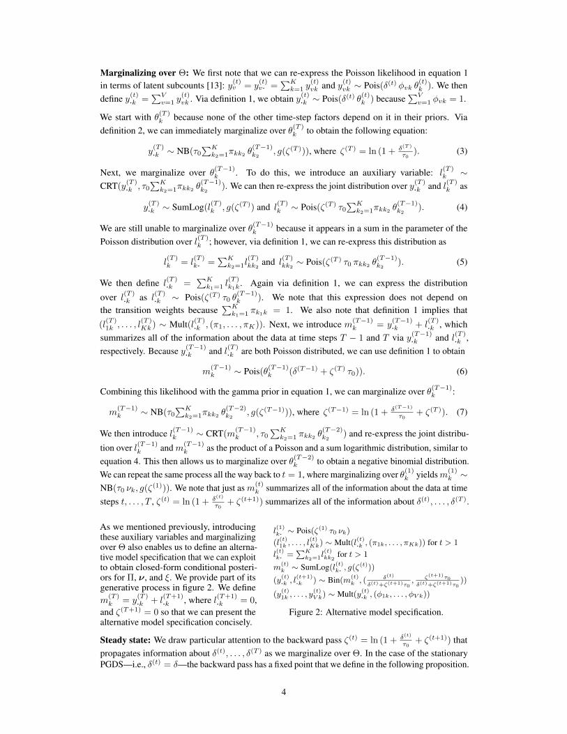
l(1)k· ∼ Pois(ζ(1) τ0 νk)(l

(t)1k , . . . , l

(t)Kk) ∼ Mult(l(t)·k , (π1k, . . . , πKk)) for t > 1

l(t)k· =

∑Kk2=1l

(t)kk2

for t > 1

m(t)k ∼ SumLog(l(t)k· , g(ζ

(t)))

(y(t)·k , l

(t+1)·k ) ∼ Bin(m(t)

k , ( δ(t)

δ(t)+ζ(t+1)τ0, ζ(t+1)τ0δ(t)+ζ(t+1)τ0

))

(y(t)1k , . . . , y

(t)V k) ∼ Mult(y(t)·k , (φ1k, . . . , φV k))

Figure 2: Alternative model specification.

As we mentioned previously, introducingthese auxiliary variables and marginalizingover Θ also enables us to define an alterna-tive model specification that we can exploitto obtain closed-form conditional posteri-ors for Π, ν, and ξ. We provide part of itsgenerative process in figure 2. We definem

(T )k = y

(T )·k + l

(T+1)·k , where l(T+1)

·k = 0,and ζ(T+1) = 0 so that we can present thealternative model specification concisely.

Steady state: We draw particular attention to the backward pass ζ(t) = ln (1 + δ(t)

τ0+ ζ(t+1)) that

propagates information about δ(t), . . . , δ(T ) as we marginalize over Θ. In the case of the stationaryPGDS—i.e., δ(t) = δ—the backward pass has a fixed point that we define in the following proposition.

4

Proposition 1: The backward pass has a fixed point of ζ? = −W−1(− exp (−1− δτ0

))− 1− δτ0

.

The function W−1(·) is the lower real part of the Lambert W function [11]. We prove this propositionin the supplementary material. During inference, we perform the O(T ) backward pass repeatedly.The existence of a fixed point means that we can assume the stationary PGDS is in its steady state andreplace the backward pass with anO(1) computation1 of the fixed point ζ∗. To make this assumption,we must also assume that l(T+1)

·k ∼ Pois(ζ? τ0 θ(T )k ) instead of l(T+1)

·k = 0. We note that an analogoussteady-state approximation exists for the LDS and is routinely exploited to reduce computation [25].

Gibbs sampling algorithm: Given Y and the hyperparameters, Gibbs sampling involves resamplingeach auxiliary variable or model parameter from its conditional posterior. Our algorithm involves a“backward filtering” pass and a “forward sampling” pass, which together form a “backward filtering–forward sampling” algorithm. We use − \Θ(≥t) to denote everything excluding θ(t), . . . ,θ(T ).

Sampling the auxiliary variables: This step is the “backward filtering” pass. For the stationary PGDSin its steady state, we first compute ζ∗ and draw (l

(T+1)·k | −) ∼ Pois(ζ? τ0 θ

(T )k ). For the other vari-

ants of the model, we set l(T+1)·k = ζ(T+1) = 0. Then, working backward from t = T, . . . , 2, we draw

(l(t)k· | − \Θ(≥t)) ∼ CRT(y

(t)·k + l

(t+1)·k , τ0

∑Kk2=1πkk2 θ

(t−1)k2

) and (8)

(l(t)k1 , . . . , l

(t)kK | − \Θ(≥t)) ∼ Mult(l(t)k· , (

πk1 θ(t−1)1∑K

k2=1 πkk2θ(t−1)k2

, . . . ,πkK θ

(t−1)K∑K

k2=1 πkk2θ(t−1)k2

)). (9)

After using equations 8 and 9 for all k = 1, . . . ,K, we then set l(t)·k =∑Kk1=1l

(t)k1k

. For the non-steady-

state variants, we also set ζ(t) = ln (1 + δ(t)

τ0+ ζ(t+1)); for the steady-state variant, we set ζ(t) = ζ∗.

Sampling Θ: We sample Θ from its conditional posterior by performing a “forward sampling” pass,starting with θ(1). Conditioned on the values of l(2)·k , . . . , l

(T+1)·k and ζ(2), . . . , ζ(T+1) obtained via

the “backward filtering” pass, we sample forward from t = 1, . . . , T , using the following equations:

(θ(1)k | − \Θ) ∼ Gam(y

(1)·k + l

(2)·k + τ0 νk, τ0 + δ(1) + ζ(2) τ0) and (10)

(θ(t)k | − \Θ(≥t)) ∼ Gam(y

(t)·k + l

(t+1)·k + τ0

∑Kk2=1πkk2 θ

(t−1)k2

, τ0 + δ(t) + ζ(t+1) τ0). (11)

Sampling Π: The alternative model specification, with Θ marginalized out, assumes that(l

(t)1k , . . . , l

(t)Kk) ∼ Mult(l(t)·k , (π1k, . . . , πKk)). Therefore, via Dirichlet–multinomial conjugacy,

(πk | − \Θ) ∼ Dir(ν1νk +∑Tt=1l

(t)1k , . . . , ξνk +

∑Tt=1l

(t)kk , . . . , νKνk +

∑Tt=1l

(t)Kk). (12)

Sampling ν and ξ: We use the alternative model specification to obtain closed-form conditionalposteriors for νk and ξ. First, we marginalize over πk to obtain a Dirichlet–multinomial distribution.When augmented with a beta-distributed auxiliary variable, the Dirichlet–multinomial distribution isproportional to the negative binomial distribution [26]. We draw such an auxiliary variable, which weuse, along with negative binomial augmentation schemes, to derive closed-form conditional posteriorsfor νk and ξ. We provide these posteriors, along with their derivations, in the supplementary material.

We also provide the conditional posteriors for the remaining model parameters—Φ, δ(1), . . . , δ(T ),and β—which we obtain via Dirichlet–multinomial, gamma–Poisson, and gamma–gamma conjugacy.

4 Experiments

In this section, we compare the predictive performance of the PGDS to that of the LDS and thatof gamma process dynamic Poisson factor analysis (GP-DPFA) [22]. GP-DPFA models a singlecount in Y as y(t)v ∼ Pois(

∑Kk=1 λk φvk θ

(t)k ), where each component’s time-step factors evolve

as a simple gamma Markov chain, independently of those belonging to the other components:θ(t)k ∼ Gam(θ

(t−1)k , c(t)). We consider the stationary variants of all three models.2 We used five data

sets, and tested each model on two time-series prediction tasks: smoothing—i.e., predicting y(t)v given1Several software packages contain fast implementations of the Lambert W function.2We used the pykalman Python library for the LDS and implemented GP-DPFA ourselves.

5

y(1)v , . . . , y

(t−1)v , y

(t+1)v , . . . , y

(T )v —and forecasting—i.e., predicting y(T+s)

v given y(1)v , . . . , y(T )v for

some s ∈ 1, 2, . . . [27]. We provide brief descriptions of the data sets below before reporting results.

Global Database of Events, Language, and Tone (GDELT): GDELT is an international relations dataset consisting of country-to-country interaction events of the form “country i took action a towardcountry j at time t,” extracted from news corpora. We created five count matrices, one for each yearfrom 2001 through 2005. We treated directed pairs of countries i→j as features and counted thenumber of events for each pair during each day. We discarded all pairs with fewer than twenty-fivetotal events, leaving T = 365, around V ≈ 9, 000, and three to six million events for each matrix.

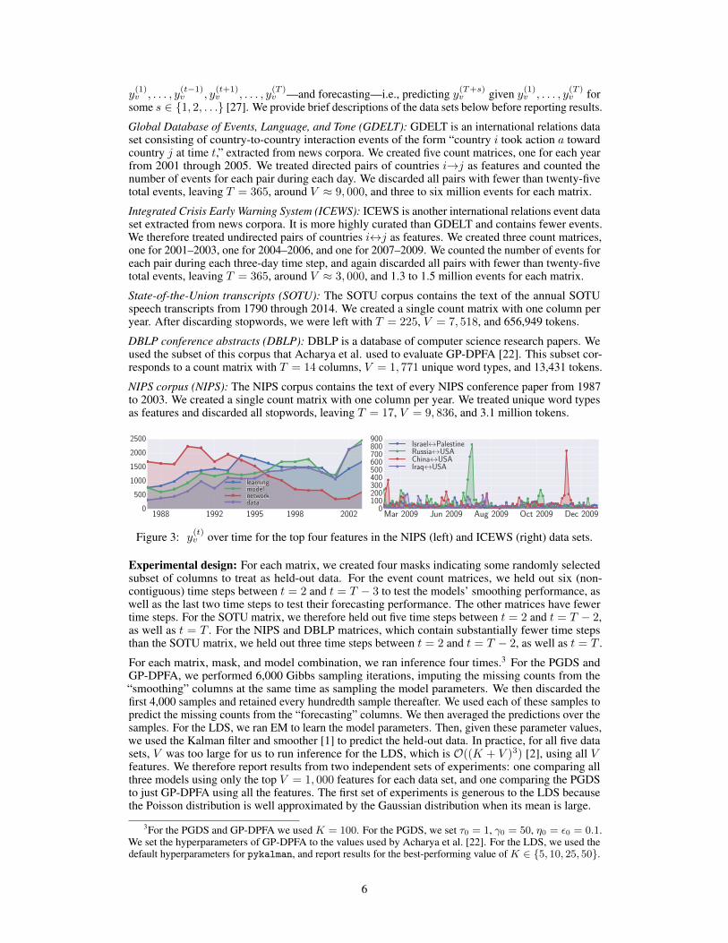
Integrated Crisis Early Warning System (ICEWS): ICEWS is another international relations event dataset extracted from news corpora. It is more highly curated than GDELT and contains fewer events.We therefore treated undirected pairs of countries i↔j as features. We created three count matrices,one for 2001–2003, one for 2004–2006, and one for 2007–2009. We counted the number of events foreach pair during each three-day time step, and again discarded all pairs with fewer than twenty-fivetotal events, leaving T = 365, around V ≈ 3, 000, and 1.3 to 1.5 million events for each matrix.

State-of-the-Union transcripts (SOTU): The SOTU corpus contains the text of the annual SOTUspeech transcripts from 1790 through 2014. We created a single count matrix with one column peryear. After discarding stopwords, we were left with T = 225, V = 7, 518, and 656,949 tokens.

DBLP conference abstracts (DBLP): DBLP is a database of computer science research papers. Weused the subset of this corpus that Acharya et al. used to evaluate GP-DPFA [22]. This subset cor-responds to a count matrix with T = 14 columns, V = 1, 771 unique word types, and 13,431 tokens.

NIPS corpus (NIPS): The NIPS corpus contains the text of every NIPS conference paper from 1987to 2003. We created a single count matrix with one column per year. We treated unique word typesas features and discarded all stopwords, leaving T = 17, V = 9, 836, and 3.1 million tokens.

1988 1992 1995 1998 20020

500

1000

1500

2000

2500

Mar 2009 Jun 2009 Aug 2009 Oct 2009 Dec 20090

100200300400500600700800900

Israel↔PalestineRussia↔USAChina↔USAIraq↔USA

Figure 3: y(t)v over time for the top four features in the NIPS (left) and ICEWS (right) data sets.

Experimental design: For each matrix, we created four masks indicating some randomly selectedsubset of columns to treat as held-out data. For the event count matrices, we held out six (non-contiguous) time steps between t = 2 and t = T − 3 to test the models’ smoothing performance, aswell as the last two time steps to test their forecasting performance. The other matrices have fewertime steps. For the SOTU matrix, we therefore held out five time steps between t = 2 and t = T − 2,as well as t = T . For the NIPS and DBLP matrices, which contain substantially fewer time stepsthan the SOTU matrix, we held out three time steps between t = 2 and t = T − 2, as well as t = T .

For each matrix, mask, and model combination, we ran inference four times.3 For the PGDS andGP-DPFA, we performed 6,000 Gibbs sampling iterations, imputing the missing counts from the“smoothing” columns at the same time as sampling the model parameters. We then discarded thefirst 4,000 samples and retained every hundredth sample thereafter. We used each of these samples topredict the missing counts from the “forecasting” columns. We then averaged the predictions over thesamples. For the LDS, we ran EM to learn the model parameters. Then, given these parameter values,we used the Kalman filter and smoother [1] to predict the held-out data. In practice, for all five datasets, V was too large for us to run inference for the LDS, which is O((K + V )3) [2], using all Vfeatures. We therefore report results from two independent sets of experiments: one comparing allthree models using only the top V = 1, 000 features for each data set, and one comparing the PGDSto just GP-DPFA using all the features. The first set of experiments is generous to the LDS becausethe Poisson distribution is well approximated by the Gaussian distribution when its mean is large.

3For the PGDS and GP-DPFA we used K = 100. For the PGDS, we set τ0 = 1, γ0 = 50, η0 = ε0 = 0.1.We set the hyperparameters of GP-DPFA to the values used by Acharya et al. [22]. For the LDS, we used thedefault hyperparameters for pykalman, and report results for the best-performing value of K ∈ 5, 10, 25, 50.

6

Table 1: Results for the smoothing (“S”) and forecasting (“F”) tasks. For both error measures, lowervalues are better. We also report the number of time steps T and the burstiness B of each data set.

Mean Relative Error (MRE) Mean Absolute Error (MAE)

T B Task PGDS GP-DPFA LDS PGDS GP-DPFA LDS

GDELT 365 1.27 S 2.335 ±0.19 2.951 ±0.32 3.493 ±0.53 9.366 ±2.19 9.278 ±2.01 10.098 ±2.39

F 2.173 ±0.41 2.207 ±0.42 2.397 ±0.29 7.002 ±1.43 7.095 ±1.67 7.047 ±1.25

ICEWS 365 1.10 S 0.808 ±0.11 0.877 ±0.12 1.023 ±0.15 2.867 ±0.56 2.872 ±0.56 3.104 ±0.60

F 0.743 ±0.17 0.792 ±0.17 0.937 ±0.31 1.788 ±0.47 1.894 ±0.50 1.973 ±0.62

SOTU 225 1.45 S 0.233 ±0.01 0.238 ±0.01 0.260 ±0.01 0.408 ±0.01 0.414 ±0.01 0.448 ±0.00

F 0.171 ±0.00 0.173 ±0.00 0.225 ±0.01 0.323 ±0.00 0.314 ±0.00 0.370 ±0.00

DBLP 14 1.64 S 0.417 ±0.03 0.422 ±0.05 0.405 ±0.05 0.771 ±0.03 0.782 ±0.06 0.831 ±0.01

F 0.322 ±0.00 0.323 ±0.00 0.369 ±0.06 0.747 ±0.01 0.715 ±0.00 0.943 ±0.07

NIPS 17 0.33 S 0.415 ±0.07 0.392 ±0.07 1.609 ±0.43 29.940 ±2.95 28.138 ±3.08 108.378 ±15.44

F 0.343 ±0.01 0.312 ±0.00 0.642 ±0.14 62.839 ±0.37 52.963 ±0.52 95.495 ±10.52

Results: We used two error measures—mean relative error (MRE) and mean absolute error (MAE)—to compute the models’ smoothing and forecasting scores for each matrix and mask combination. Wethen averaged these scores over the masks. For the data sets with multiple matrices, we also averagedthe scores over the matrices. The two error measures differ as follows: MRE accommodates thescale of the data, while MAE does not. This is because relative error—which we define as |y

(t)v −y

(t)v |

1+y(t)v

,

where y(t)v is the true count and y(t)v is the prediction—divides the absolute error by the true count andthus penalizes overpredictions more harshly than underpredictions. MRE is therefore an especiallynatural choice for data sets that are bursty—i.e., data sets that exhibit short periods of activity that farexceed their mean. Models that are robust to these kinds of overdispersed temporal patterns are lesslikely to make overpredictions following a burst, and are therefore rewarded accordingly by MRE.

In table 1, we report the MRE and MAE scores for the experiments using the top V = 1, 000 features.We also report the average burstiness of each data set. We define the burstiness of feature v in matrixY to be Bv = 1

T−1∑T−1t=1

|y(t+1)v −y(t)v |

µv, where µv = 1

T

∑Tt=1 y

(t)v . For each data set, we calculated

the burstiness of each feature in each matrix, and then averaged these values to obtain an averageburstiness score B. The PGDS outperformed the LDS and GP-DPFA on seven of the ten predictiontasks when we used MRE to measure the models’ performance; when we used MAE, the PGDSoutperformed the other models on five of the tasks. In the supplementary material, we also report theresults for the experiments comparing the PGDS to GP-DPFA using all the features. The superiorityof the PGDS over GP-DPFA is even more pronounced in these results. We hypothesize that thedifference between these models is related to the burstiness of the data. For both error measures, theonly data set for which GP-DPFA outperformed the PGDS on both tasks was the NIPS data set. Thisdata set has a substantially lower average burstiness score than the other data sets. We provide visualevidence in figure 3, where we display y(t)v over time for the top four features in the NIPS and ICEWSdata sets. For the former, the features evolve smoothly; for the latter, they exhibit bursts of activity.

Exploratory analysis: We also explored the latent structure inferred by the PGDS. Because itsparameters are positive, they are easy to interpret. In figure 1, we depict three components inferredfrom the NIPS data set. By examining the time-step factors and feature factors for these components,we see that they capture the decline of research on neural networks between 1987 and 2003, as wellas the rise of Bayesian methods in machine learning. These patterns match our prior knowledge.

In figure 4, we depict the three components with the largest component weights inferred by the PGDSfrom the 2003 GDELT matrix. The top component is in blue, the second is in green, and the thirdis in red. For each component, we also list the sixteen features (directed pairs of countries) withthe largest feature factors. The top component (blue) is most active in March and April, 2003. Itsfeatures involve USA, Iraq (IRQ), Great Britain (GBR), Turkey (TUR), and Iran (IRN), among others.This component corresponds to the 2003 invasion of Iraq. The second component (green) exhibits anoticeable increase in activity immediately after April, 2003. Its top features involve Israel (ISR),Palestine (PSE), USA, and Afghanistan (AFG). The third component exhibits a large burst of activity

7

Jan 2003 Mar 2003 May 2003 Aug 2003 Oct 2003 Dec 20031

2

3

4

5

6

Figure 4: The time-step factors for the top three components inferred by the PGDS from the 2003GDELT matrix. The top component is in blue, the second is in green, and the third is in red. For eachcomponent, we also list the features (directed pairs of countries) with the largest feature factors.

in August, 2003, but is otherwise inactive. Its top features involve North Korea (PRK), South Korea(KOR), Japan (JPN), China (CHN), Russia (RUS), and USA. This component corresponds to thesix-party talks—a series of negotiations between these six countries for the purpose of dismantlingNorth Korea’s nuclear program. The first round of talks occurred during August 27–29, 2003.

0 1 2 3 4 5 6 7 8 9

01

23

45

67

89

0123456

Figure 5: The latent tran-sition structure inferred bythe PGDS from the 2003GDELT matrix. Top: Thecomponent weights for thetop ten components, in de-creasing order from left toright; two of the weights aregreater than one. Bottom:The transition weights in thecorresponding subset of thetransition matrix. This struc-ture means that all compo-nents are likely to transitionto the top two components.

In figure 5, we also show the component weights for the top ten com-ponents, along with the corresponding subset of the transition matrixΠ. There are two components with weights greater than one: the com-ponents that are depicted in blue and green in figure 4. The transitionweights in the corresponding rows of Π are also large, meaning thatother components are likely to transition to them. As we mentionedpreviously, the GDELT data set was extracted from news corpora.Therefore, patterns in the data primarily reflect patterns in media cov-erage of international affairs. We therefore interpret the latent structureinferred by the PGDS in the following way: in 2003, the media brieflycovered various major events, including the six-party talks, beforequickly returning to a backdrop of the ongoing Iraq war and Israeli–Palestinian relations. By inferring the kind of transition structuredepicted in figure 5, the PGDS is able to model persistent, long-termtemporal patterns while accommodating the burstiness often inherentto real-world count data. This ability is what enables the PGDS toachieve superior predictive performance over the LDS and GP-DPFA.

5 Summary

We introduced the Poisson–gamma dynamical system (PGDS)—a newBayesian nonparametric model for sequentially observed multivariatecount data. This model supports the expressive transition structureof the linear dynamical system, and naturally handles overdisperseddata. We presented a novel MCMC inference algorithm that remainsefficient for high-dimensional data sets, advancing recent work on aug-mentation schemes for inference in negative binomial models. Finally,we used the PGDS to analyze five real-world data sets, demonstratingthat it exhibits superior smoothing and forecasting performance overtwo baseline models and infers highly interpretable latent structure.

Acknowledgments

We thank David Belanger, Roy Adams, Kostis Gourgoulias, Ben Marlin, Dan Sheldon, and TimVieira for many helpful conversations. This work was supported in part by the UMass Amherst CIIRand in part by NSF grants SBE-0965436 and IIS-1320219. Any opinions, findings, conclusions, orrecommendations are those of the authors and do not necessarily reflect those of the sponsors.

8

References[1] R. E. Kalman. A new approach to linear filtering and prediction problems. Journal of Basic

Engineering, 82(1):35–45, 1960.[2] Z. Ghahramani and S. T. Roweis. Learning nonlinear dynamical systems using an EM algorithm.

In Advances in Neural Information Processing Systems, pages 431–437, 1998.[3] S. S. Haykin. Kalman Filtering and Neural Networks. 2001.[4] P. McCullagh and J. A. Nelder. Generalized linear models. 1989.[5] M. G. Bulmer. On fitting the Poisson lognormal distribution to species-abundance data. Biomet-

rics, pages 101–110, 1974.[6] D. M. Blei and J. D. Lafferty. Dynamic topic models. In Proceedings of the 23rd International

Conference on Machine Learning, pages 113–120, 2006.[7] L. Charlin, R. Ranganath, J. McInerney, and D. M. Blei. Dynamic Poisson factorization. In

Proceedings of the 9th ACM Conference on Recommender Systems, pages 155–162, 2015.[8] J. H. Macke, L. Buesing, J. P. Cunningham, B. M. Yu, K. V. Krishna, and M. Sahani. Empirical

models of spiking in neural populations. In Advances in Neural Information Processing Systems,pages 1350–1358, 2011.

[9] J. Kleinberg. Bursty and hierarchical structure in streams. Data Mining and KnowledgeDiscovery, 7(4):373–397, 2003.

[10] M. Zhou and L. Carin. Augment-and-conquer negative binomial processes. In Advances inNeural Information Processing Systems, pages 2546–2554, 2012.

[11] R. Corless, G. Gonnet, D. E. G. Hare, D. J. Jeffrey, and D. E. Knuth. On the LambertW function.Advances in Computational Mathematics, 5(1):329–359, 1996.

[12] J. Canny. GaP: A factor model for discrete data. In Proceedings of the 27th Annual InternationalACM SIGIR Conference on Research and Development in Information Retrieval, pages 122–129,2004.

[13] A. T. Cemgil. Bayesian inference for nonnegative matrix factorisation models. ComputationalIntelligence and Neuroscience, 2009.

[14] M. Zhou, L. Hannah, D. Dunson, and L. Carin. Beta-negative binomial process and Poissonfactor analysis. In Proceedings of the 15th International Conference on Artificial Intelligenceand Statistics, 2012.

[15] P. Gopalan, J. Hofman, and D. Blei. Scalable recommendation with Poisson factorization. InProceedings of the 31st Conference on Uncertainty in Artificial Intelligence, 2015.

[16] T. S. Ferguson. A Bayesian analysis of some nonparametric problems. The Annals of Statistics,1(2):209–230, 1973.

[17] M. Zhou. Infinite edge partition models for overlapping community detection and link prediction.In Proceedings of the 18th International Conference on Artificial Intelligence and Statistics,pages 1135–1143, 2015.

[18] M. Zhou, Y. Cong, and B. Chen. Augmentable gamma belief networks. Journal of MachineLearning Research, 17(163):1–44, 2016.

[19] M. E. Basbug and B. Engelhardt. Hierarchical compound Poisson factorization. In Proceedingsof the 33rd International Conference on Machine Learning, 2016.

[20] R. M. Adelson. Compound Poisson distributions. OR, 17(1):73–75, 1966.[21] M. Zhou and L. Carin. Negative binomial process count and mixture modeling. IEEE Transac-

tions on Pattern Analysis and Machine Intelligence, 37(2):307–320, 2015.[22] A. Acharya, J. Ghosh, and M. Zhou. Nonparametric Bayesian factor analysis for dynamic

count matrices. Proceedings of the 18th International Conference on Artificial Intelligence andStatistics, 2015.

[23] J. F. C. Kingman. Poisson Processes. Oxford University Press, 1972.[24] D. B. Dunson and A. H. Herring. Bayesian latent variable models for mixed discrete outcomes.

Biostatistics, 6(1):11–25, 2005.[25] W. J. Rugh. Linear System Theory. Pearson, 1995.[26] M. Zhou. Nonparametric Bayesian negative binomial factor analysis. arXiv:1604.07464.[27] J. Durbin and S. J. Koopman. Time Series Analysis by State Space Methods. Oxford University

Press, 2012.

9

Supplementary Material for“Poisson–Gamma Dynamical Systems”

Aaron ScheinCollege of Information and Computer Sciences

University of Massachusetts AmherstAmherst, MA 01003

aschein@cs.umass.edu

Mingyuan ZhouMcCombs School of Business

The University of Texas at AustinAustin, TX 78712

mingyuan.zhou@mccombs.utexas.edu

Hanna WallachMicrosoft Research New York641 Avenue of the Americas

New York, NY 10011hanna@dirichlet.net

1 Bayesian Nonparametric Interpretation

As K → ∞, the component weights and their corresponding feature factor vectors constitute adraw G =

∑∞k=1 νk1φk

from a gamma process GamP (G0, β), where β is a scale parameter andG0 is a finite and continuous base measure over a complete separable metric space Ω [1]. Modelsbased on the gamma process have an inherent shrinkage mechanism because the number of atomswith weights greater than ε > 0 follows a Poisson distribution with a finite mean—specifically,Pois(γ0

∫∞ε

dν ν−1 exp (−β ν)), where γ0 = G0(Ω) is the total mass under the base measure.

This interpretation enables us to view the priors over Π and Θ as a novel stochastic processes.Because of the relationship between the Dirichlet and gamma distributions [1], we can equiva-lently express the prior over the kth column of Π as πk1k =

λk1k∑Kk2=1 λk1k2

for k1 = 1, . . . ,K,

where λkk ∼ Gam(ξ νk, c), and λk1k ∼ Gam(νk1νk, c) for k1 6= k are auxiliary variables. AsK → ∞,

∑∞k1=1

∑∞k2=1 λk1k21(φk1

,φk2) is a draw from a relational gamma process [2] and∑∞

k1=1

∑∞k2=1 πk1k21(φk1

,φk2) is a draw from a column-normalized relational gamma process.

Given τ0, Π, and G =∑∞k=1 νk 1φk

, the prior over Θ is a recurrent gamma process—a sequence ofgamma processes, each defined over the product space R+ × Ω—defined recursively as follows:

G(t) =∑∞k=1θ

(t)k 1φk

∼ GamP(H(t), τ0) and H(t) =∑∞k=1(τ0

∑∞k2=1πkk2 θ

(t−1)k2

)1φk, (1)

where H(1) = τ0G. This recursive sequence of gamma processes will never produce a draw withinfinite mass at some time step t, which would make H(t+1) infinite and violate the entire definition.

Theorem 1: The expected sum of θ(t) is finite and equal to E[∑∞k=1 θ

(t)k ] = γ0

β .

By linearity of expectation, the definition of the recurrent gamma process, and∑∞k1=1 πk1k = 1,

E[∑∞k=1θ

(t)k ] =

∑∞k=1E[θ

(t)k ] =

∑∞k=1E[

∑∞k2=1πkk2 θ

(t−1)k2

] = E[∑∞k=1θ

(t−1)k=1 ]. (2)

Then, by induction and the definition of the recurrent gamma process,

E[∑∞k=1θ

(t−1)k ] = . . . = E[

∑∞k=1θ

(1)k ] = γ0

β . (3)

30th Conference on Neural Information Processing Systems (NIPS 2016), Barcelona, Spain.

2 Proof of Proposition 1

Proposition 1: The backward pass has a fixed point of ζ? = −W−1(− exp (−1− δτ0

))− 1− δτ0

.

If a fixed point exists, then it must satisfy the following equation:

ζ? = ln (1 + δτ0

+ ζ?) (4)

exp (ζ?) = 1 + δτ0

+ ζ? (5)

1 = (1 + δτ0

+ ζ?) exp (−ζ?) (6)

−1 = (−1− δτ0− ζ?) exp (−ζ?) (7)

− exp (−1− δτ0

) = (−1− δτ0− ζ?) exp (−ζ?) exp (−1− δ

τ0) (8)

− exp (−1− δτ0

) = (−1− δτ0− ζ?) exp (−1− δ

τ0− ζ?). (9)

However, y = x exp (x) is equivalent to x = W(y), so

(−1− δτ0− ζ?) = W(− exp (−1− δ

τ0)) (10)

ζ? = −W(− exp (−1− δτ0

))− 1− δτ0. (11)

There are two branches of the Lambert W function. The lower branch decreases fromW−1 (− exp (−1)) = −1 to W−1 (0) = −∞, while the principal branch increases fromW0 (− exp (−1)) = −1 to W0 (0) = 0 and beyond. Because ζ? must be positive, we therefore have

ζ? = −W−1(− exp (−1− δτ0

))− 1− δτ0. (12)

3 MCMC Inference

Definition 1: If y· =∑Nn=1 yn, where yn ∼ Pois(θn) are independent Poisson-distributed random

variables, then (y1, . . . , yN ) ∼ Mult(y·, ( θ1∑Nn=1 θn

, . . . , θN∑Nn=1 θn

)) and y· ∼ Pois(∑Nn=1 θn) [3, 4].

Sampling the latent subcounts: Via definition 1,

(y(t)v1 , . . . , y

(t)vK | −) ∼ Mult(y(t)v , (

φv1 θ(t)1∑K

k2=1 φvk θ(t)k

, . . . ,φvK θ

(t)K∑K

k2=1 φvk θ(t)k

)) (13)

Sampling Φ: Via Dirichlet–multinomial conjugacy,

(φk | −) ∼ Dir(η0 +∑Tt=1y

(t)1k , . . . , η0 +

∑Tt=1y

(t)V k). (14)

Sampling δ(1), . . . , δ(T ): Via gamma–Poisson conjugacy,

(δ(t) | −) ∼ Gamma(ε0 +∑Vv=1y

(t)v , ε0 +

∑Kk=1θ

(t)k ) (15)

Sampling δ (stationary variant): Also via gamma–Poisson conjugacy,

(δ | −) ∼ Gamma(ε0 +

∑Tt=1

∑Vv=1y

(t)v , ε0 +

∑Tt=1

∑Kk=1 θ

(t)k

). (16)

Sampling β: Via gamma–gamma conjugacy,

(β | −) ∼ Gamma(ε0 + γ0, ε0 +∑Kk=1νk). (17)

Sampling ν and ξ: To obtain closed-form conditional posteriors for νk and ξ, we start with

(l(·)1k , . . . , l

(·)kk , . . . , l

(·)Kk) ∼ DirMult(l(·)·k , (ν1νk, . . . , ξνk, . . . , νKνk)), (18)

where l(·)k1k =∑Tt=1 l

(t)k1k

and l(·)·k =∑Tt=1

∑Kk1=1 l

(t)k1k

. As noted previously by Zhou [5], whenaugmented with a beta-distributed auxiliary variable, the Dirichlet–multinomial distribution is propor-tional to the negative binomial distribution. We therefore draw a beta-distributed auxiliary variable:

qk ∼ Beta(l(·)·k , νk (ξ +

∑k1 6=kνk1)). (19)

2

Conditioned on qk, we then have

l(·)kk ∼ NB(ξ νk, qk) and l

(·)k1k∼ NB(νk1νk, qk) (20)

for k1 6= k. Next, we introduce the following auxiliary variables:

hkk ∼ CRT(l(·)kk , ξ νk) and hk1k ∼ CRT(l

(·)k1k

, νk1νk) (21)

for k1 6= k. We can then re-express the joint distribution over the variables in equations 20 and 21 as

l(·)kk ∼ SumLog(hkk, qk) and l

(·)k1k∼ SumLog(hk1k, qk) (22)

and

hkk ∼ Pois(−ξ νk ln (1− qk)) and hk1k ∼ Pois(−νk1νk ln (1− qk)). (23)

Then, via gamma–Poisson conjugacy,

(ξ | − \Θ,πk) ∼ Gam(γ0K +∑Kk=1hkk, β −

∑Kk=1νk ln (1− qk)). (24)

Next, because l(1)k· ∼ Pois(ζ(1) τ0 νk) also depends on νk, we introduce

nk = hkk +∑k1 6=khk1k +

∑k2 6=khkk2 + l

(1)k· . (25)

Then, via definition 1, we have

nk ∼ Pois(νk ρk), (26)

where

ρk = − ln (1− qk) (ξ +∑k1 6=kνk1)−

∑k2 6=k ln (1− qk2) νk2 + ζ(1)τ0. (27)

Finally, via gamma–Poisson conjugacy,

(νk | − \Θ,πk) ∼ Gam(γ0β

+ nk, β + ρk). (28)

4 Additional Results

Polyphonic music (PM): To test the models’ predictive performance for binary observations, we useda polyphonic music sequence data set [6]. We created binary matrices for the first forty-four songs inthis data set. Each matrix has one column per time step and one row for each key on the piano—i.e.,T = 111 to 3, 155 and V = 88. A single observation b(t)v = 1 means that key v was played at time t.

Table 1: Smoothing scores (higheris better) for the binary matrices.

AUC

Mask LDS GP-DPFA PGDS

PM 10% 0.94 0.92 0.93PM 20% 0.93 0.91 0.93PM 30% 0.93 0.91 0.92

For each matrix, we created six masks indicating some subsetof columns (10%, 20%, and 30%, randomly selected) totreat as held-out data. We only tested the models’ smoothingperformance because the last time steps are often empty. Foreach matrix, mask, and model combination, we ran inferenceand imputed the missing data, as described in section 4 ofthe main paper. For both the PGDS and GP-DPFA, we usedthe Bernoulli–Poisson distribution to link the observationsto latent Poisson counts [2]. We applied the LDS directly;despite being misspecified, the LDS often performs well forbinary data [7]. We used AUC [8] to compute the the models’smoothing scores (higher is better) for each inference run, andthen averaged the scores over the runs, the masks with the same percentage of held-out data, andthe matrices. We report our results in table 1. For the LDS, we only report the scores for the best-performing value of K. For all three models, performance degraded as we held out more data. TheLDS and the PGDS, both of which have an expressive transition structure, outperformed GP-DPFA.

3

Table 2: Results for the smoothing (“S”) and forecasting (“F”) tasks using all the features. Lowervalues are better. We also report the number of time steps T and the burstiness B of each data set.

Mean Relative Error Mean Absolute Error

T B Task PGDS GP-DPFA PGDS GP-DPFA

GDELT 365 1.71 S 0.428 ±0.06 0.617 ±0.06 1.491 ±0.22 1.599 ±0.21

F 0.432 ±0.09 0.494 ±0.08 1.224 ±0.19 1.263 ±0.21

ICEWS 365 1.26 S 0.334 ±0.02 0.372 ±0.01 1.003 ±0.13 1.021 ±0.14

F 0.299 ±0.05 0.313 ±0.05 0.646 ±0.13 0.673 ±0.14

SOTU 225 1.49 S 0.216 ±0.00 0.226 ±0.00 0.365 ±0.00 0.374 ±0.00

F 0.172 ±0.00 0.169 ±0.00 0.295 ±0.00 0.289 ±0.00

DBLP 14 1.73 S 0.370 ±0.00 0.356 ±0.00 0.604 ±0.00 0.591 ±0.00

F 0.370 ±0.00 0.408 ±0.00 0.778 ±0.00 0.790 ±0.00

NIPS 17 0.89 S 2.133 ±0.00 1.199 ±0.00 9.375 ±0.00 7.893 ±0.00

F 1.173 ±0.00 0.949 ±0.00 15.065 ±0.00 12.445 ±0.00

References[1] T. S. Ferguson. A Bayesian analysis of some nonparametric problems. The Annals of Statistics,

1(2):209–230, 1973.[2] M. Zhou. Infinite edge partition models for overlapping community detection and link prediction.

In Proceedings of the 18th International Conference on Artificial Intelligence and Statistics,pages 1135–1143, 2015.

[3] J. F. C. Kingman. Poisson Processes. Oxford University Press, 1972.[4] D. B. Dunson and A. H. Herring. Bayesian latent variable models for mixed discrete outcomes.

Biostatistics, 6(1):11–25, 2005.[5] M. Zhou. Nonparametric Bayesian negative binomial factor analysis. arXiv:1604.07464.[6] N. Boulanger-Lewandowski, Y. Bengio, and P. Vincent. Modeling temporal dependencies in

high-dimensional sequences: Application to polyphonic music generation and transcription. InProceedings of the 29th International Conference on Machine Learning, 2012.

[7] D. Belanger and S. Kakade. A linear dynamical system model for text. In Proceedings of the32nd International Conference on Machine Learning, 2015.

[8] C. X. Ling, J. Huang, and H. Zhang. AUC: A statistically consistent and more discriminatingmeasure than accuracy. In Proceedings of the 18th International Joint Conference on ArtificialIntelligence, pages 519–524, 2003.

4