policy insight 9 - atlanta regional...
TRANSCRIPT

Model Documentation – Version 9.5 i
Policy Insight 9.5
Model Documentation
©2007 Regional Economic Models, Inc.
Model Documentation – Version 9.5 ii
Table of Contents
Chapter 1: The REMI Economic Geography Forecasting and Policy Analysis Model1 Chapter 2: Demographic Component of the REMI Model........................................47 Chapter 3: Data Sources and Estimation Procedures...............................................51 Chapter 4: Chained vs. Fixed Real Dollars in the REMI Model ...............................73 Chapter 5: State And Local Government Employment And Final Demand.............75 Chapter 6: Predicted Revenue & Expenditure Effects ..............................................80 Chapter 7: Using the Fiscal Module in REMI Policy Insight.....................................82 Chapter 8: Decomposing Policy Effects On Employment, Wages, And Prices By
Income Groups ..................................................................................................86 Chapter 9: The Structural Consumption Equation for REMI Policy Insight Version 9.5
– George Treyz, Frederick Treyz, Nick Mata, Sherri Lawrence, Jerry Hayes .....89 Chapter 10: Consumption Equations for a Multiregional Forecasting and Policy
Analysis Model – George Treyz and Lisa Petraglia; Regional Science Perspectives in Economic Analysis, 2001 ................................................................................117
Chapter 11: Economic Implications of Congestion – Glen Weisbrod, Donald Vary, and George Treyz; NCHRP, Report 436, 2001 .................................................118
Chapter 12: An Evolutionary New Economic Geography Model – Wei Fan, Frederick Treyz, and George Treyz; Journal of Regional Science, 2000 ............................119
Chapter 13: Monopolistic Competition Estimates of Interregional Trade Flows in Services – Frederick Treyz and Jim Bumgardner; Regional Cohesion and Competition in the Age of Globalization, 2000 ....................................................120
Chapter 14: The REMI Multiregional U.S. Policy Analysis Model – Frederick Treyz and George Treyz............................................................................................121
Chapter 15: Policy Analysis Applications of REMI Economic Forecasting and Simulation Models – George Treyz; International Journal of Public Administration, 1995 122
Chapter 16: Forecasting the Effects of Electric Utility Deregulation: A Hypothetical Scenario for New Jersey – Frederick Treyz and Lisa Petraglia; The Journal of Business Forecasting, 1997.................................................................................123
Chapter 17: Regional Economic Modeling: A Systematic Approach to Economic Forecasting and Policy Analysis – George I. Treyz; 1993......................................................124
Chapter 18: Multiregional Stock Adjustment Equations of Residential and Nonresidential Investment in Structures – Dan S. Rickman, G. Shao, and George I. Treyz; Journal of Regional Science, 1993........................................................125
Chapter 19: Alternative Labor Market Closures in a Regional Model – Dan S. Rickman and George I. Treyz; Growth and Change, 1993 ................................126
Chapter 20: The Dynamics of U.S. Internal Migration – George I. Treyz, et al; The Review of Economics and Statistics, 1993 ...........................................................127

Model Documentation – Version 9.5 iii
Chapter 21: Building U.S. National and Regional Forecasting and Simulation Models – Gang Shao and George I. Treyz; Economics Systems Research, 1993 .............128
Chapter 22: The REMI Economic-Demographic Forecasting and Simulation Model – G.I. Treyz, D.S. Rickman, G. Shao; International Regional Science Review, 1992129
Chapter 23: Migration, Regional Equilibrium, and the Estimation of Compensating Differentials – Michael J. Greenwood, et al; American Economic Review, 1991130
Chapter 24: List of Published Papers and Articles in REMI Files - By Topic with File Numbers..........................................................................................................131

Model Documentation – Version 9.5 iv
Preface
Economic Documentation for REMI Policy Insight The first paper in this volume is “The REMI Economic Geography Forecasting and Policy Analysis Model.” It provides the key diagrams and equations for documenting the REMI model. The equations in this paper supersede those in previous model documentation for all U.S. and International REMI Policy Insight versions. Values of your model’s parameters are available in REMI Policy Insight by clicking on the View Parameters option in the Data menu. However, some aspects of the model and its data require more detail. These follow the first paper as chapters 2-9 in the Table of Contents. Next, the abstracts and front pages of selected articles, providing background and research details, authored or co-authored by REMI staff, are provided. These are listed as items 10-23 in the Table of Contents and are available from REMI without charge by request. Finally, a list of published articles listed by topic, also available from REMI, is included. Again, all of the references are available without charge.
Further information is also available at www.remi.com.
Model Documentation – Version 9.5 1
Chapter 1: The REMI Economic Geography Forecasting and Policy Analysis Model
Table of Contents
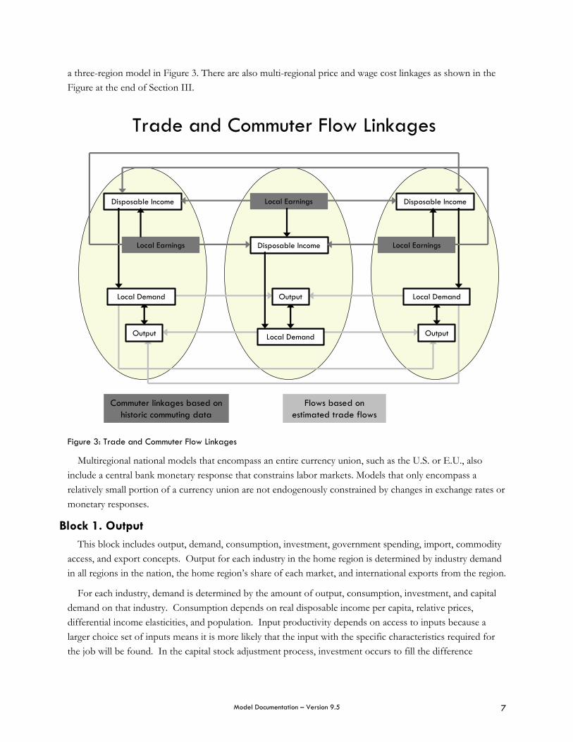
I. Introduction..................................................................................................................2 II. Overview of the Model...............................................................................................4
Block 1. Output ................................................................................................................................7 Block 2. Labor and Capital Demand .........................................................................................8 Block 3. Population and Labor Force .........................................................................................8 Block 4. Wages, Prices and Costs...............................................................................................8 Block 5. Market Shares.................................................................................................................9
III. Detailed Diagrammatic and Verbal Description ......................................................10 Block 1. Output............................................................................................................................ 10 Block 2. Labor and Capital Demand ...................................................................................... 15 Block 3. Population and Labor Force ...................................................................................... 17 Block 4. Wages, Prices, and Costs........................................................................................... 19 Block 5. Market Shares.............................................................................................................. 20
IV. Block by Block Equations .......................................................................................22 Block 1 - Output ........................................................................................................................... 22
Output Equations...................................................................................................................... 22 Consumption Equations............................................................................................................ 24 Real Disposable Income Equations ....................................................................................... 25 Investment Equations................................................................................................................ 28 Government Spending Equations.......................................................................................... 29
Block 2 – Labor and Capital Demand ..................................................................................... 30 Labor Demand Equations ....................................................................................................... 30 Capital Demand Equations .................................................................................................... 34 Demand for Fuel ...................................................................................................................... 35
Block 3 – Population and Labor Force..................................................................................... 35 Labor Force Equations............................................................................................................. 37
Block 4 – Wages, Prices and Costs ...................................................................................... 38 Production Costs ....................................................................................................................... 38 Delivered Prices ....................................................................................................................... 39 Cost of Equipment.................................................................................................................... 39 Consumption Deflator.............................................................................................................. 40 Consumer Price Index Based on Delivered Costs............................................................... 40 Consumer Price to be Used for Potential In or Out Migrants .......................................... 40 Housing Price Equations .......................................................................................................... 40 The Compensation Equation................................................................................................... 41
Block 5 - Market Shares ............................................................................................................. 43 List of References..........................................................................................................46

Model Documentation – Version 9.5 2
I. Introduction
Since “all politics are local,” the effects of policies on sub-national areas have always been of great interest in the policy-making process. If anything, the concern about regional economies is becoming greater. The reasons for this heightened concern have to do with a combination of economic realities, changing political structures, and the influence of economic research that has emerged over the last decade.
First, after decades of steadily expanding economic prosperity, evidence began to suggest that lagging economies may not inevitably catch up to more advanced areas. Coastal China has continued to develop more rapidly than the interior; much of the income growth in the U.S. in the past decade has been focused in leading metropolitan areas of the Northeast, Texas, and California; and regional disparities persist in almost every European country.
Second, national economies have become more open, through both globalization and regional blocks such as NAFTA and the EU. This changing political organization forces local economic regions to compete with each other, without the national protection of industries. Thus, regions within a country may have an economy that is much stronger or weaker than the national economy as a whole. For example, the states of eastern Germany still lag far behind those of western Germany, despite the overall strength of the German economy.
Finally, the “new economic geography” (see Fujita, et al.) has focused attention on the spatial dimension of the economy. In this emerging area of research, the geographic location of an economy may be even more significant than a national boundary. In fact, the new economic geography shows how economic disparities can surface even with equal resource endowments and in the absence of trade barriers. Since history plays an important role in the development of regional economies, these new research findings also suggest that economic policies may have a significant effect on local economic growth.
In light of this interest, regional policy analysis models can play an important role in evaluating the economic effects of alternative courses of action. Model users can answer “what if” questions about the economic effects of policies in areas such as economic development, energy, transportation, the environment, and taxation. Thus, simulation models for state, provincial, and local economies can help guide decision makers in formulating strategies for these geographical areas.
REMI Policy Insight is probably the most widely applied regional economic policy analysis model. Uses of the model to predict the regional economic and demographic effects of policies cover a range of issues; some examples include electric utility restructuring in Wyoming, the construction of a new baseball park for Boston, air pollution regulations in California, and the provision of tax incentives for business expansion in Michigan. The model is used by government agencies on the national, state, and local level, as well as by private consulting firms, utilities, and universities.
The original version of the model was developed as the Massachusetts Economic Policy Analysis (MEPA, Treyz, Friedlander, and Stevens) model in 1977. It was then extended into a model that could be generalized for all states and counties in the U.S. under a grant from the National Cooperative Highway Research Program. In 1980, Regional Economic Models, Inc. (REMI) was founded to build, maintain, and advise on the use of the REMI model for individual regions. REMI was also established to further the theoretical

Model Documentation – Version 9.5 3
framework, methodology, and estimation of the model through ongoing economic research and development.
Major extensions of the initial model include the incorporation of a dynamic capital stock adjustment process (Rickman, Shao, and Treyz, 1993), migration equations with detailed demographic structure (Greenwood, Hunt, Rickman, and Treyz, 1991; Treyz, Rickman, Hunt, and Greenwood, 1993), consumption equations (Treyz and Petraglia, 2001), and endogenous labor force participation rates (Treyz, Christopher, and Lou, 1996). A multi-regional national model has also been developed that has a central bank monetary response to economic changes that occur at the regional level (Treyz and Treyz, 1997).
Recently, the model structure has been developed to include “new economic geography” assumptions. Economic geography theory explains regional and urban economies in terms of competing factors of dispersion and agglomeration. Producers and consumers are assumed to benefit from access to variety, which tends to concentrate production and the location of households. However, land is a finite resource, and high land prices and congestion tend to disperse economic activity.
Economic geography is incorporated in the model in two basic indexes. The first is the commodity access index, which predicts how productivity will be enhanced and costs reduced when firms increase access to intermediate inputs. This index is also used in the migration equation to incorporate the beneficial effect for consumers of having more access to consumer goods, which is factored into their migration decisions. The second index is the labor access index, which captures the favorable effect on labor productivity and thus labor costs when local firms have access to a wide variety of potential employees and are able to select employees whose skills best suit their needs.

Model Documentation – Version 9.5 4
II. Overview of the Model
REMI Policy Insight is a structural economic forecasting and policy analysis model. It integrates input-output, computable general equilibrium, econometric, and economic geography methodologies. The model is dynamic, with forecasts and simulations generated on an annual basis and behavioral responses to wage, price, and other economic factors.
The REMI model consists of thousands of simultaneous equations with a structure that is relatively straightforward. The exact number of equations used varies depending on the extent of industry, demographic, demand, and other detail in the specific model being used. The overall structure of the model can be summarized in five major blocks: (1) Output, (2) Labor and Capital Demand, (3) Population and Labor Supply, (4) Wages, Prices, and Costs, and (5) Market Shares. The blocks and their key interactions are shown in Figures 1 and 2.

Model Documentation – Version 9.5 5
REMI Model Linkages (Excluding Economic Geography Linkages)
State and Local Government Spending
Investment
(1) Output
Output
Exports
Consumption
Real Disposable Income
(4) Wages, Prices, and Costs
Employment Opportunity
Housing Price
Compensation Rate Composite Comp. Rate Production Costs
Composite PricesReal Comp. RateConsumer Price
Deflator
(3) Population and Labor Supply
(2) Labor & Capital Demand
Optimal Capital Stock
Employment
Labor Productivity
(5) Market Shares
Domestic Market Share
International Market Share
Population
ParticipationRate
Migration
Labor Force
Figure 1: REMI Model Linkages

Model Documentation – Version 9.5 6
Economic Geography Linkages
Intermediate Input Productivity
Intermediate Inputs (1) Output
(4) Wages, Prices, and Costs
Composite Wage
Production Costs
Composite Prices
(3) Population and Labor Supply
(2) Labor & Capital Demand
Labor Access Index
Employment
Labor Productivity
(5) Market Shares
Domestic Market Share
International Market Share
EconomicMigrants
Output
Commodity Access Index
Figure 2: Economic Geography Linkages
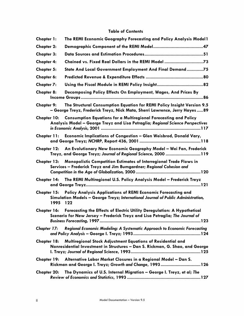
The Output block consists of output, demand, consumption, investment, government spending, exports, and imports, as well as feedback from output change due to the change in the productivity of intermediate inputs. The Labor and Capital Demand block includes labor intensity and productivity as well as demand for labor and capital. Labor force participation rate and migration equations are in the Population and Labor Supply block. The Wages, Prices, and Costs block includes composite prices, determinants of production costs, the consumption price deflator, housing prices, and the wage equations. The proportion of local, inter-regional, and export markets captured by each region is included in the Market Shares block.
Models can be built as single region, multi-region, or multi-region national models. A region is defined broadly as a sub-national area, and could consist of a state, province, county, or city, or any combination of sub-national areas. Within a large, multinational currency zone such as the European Union, models of a national economy can be built using the same economic framework employed in regional models.
Single-region models consist of an individual region, called the home region. The rest of the nation is also represented in the model. However, since the home region is only a small part of the total nation, the changes in the region do not have an endogenous effect on the variables in the rest of the nation.
Multi-regional models have interactions among regions, such as trade and commuting flows. These interactions include trade flows from each region to each of the other regions. These flows are illustrated for
Model Documentation – Version 9.5 7
a three-region model in Figure 3. There are also multi-regional price and wage cost linkages as shown in the Figure at the end of Section III.
Trade and Commuter Flow Linkages
Flows based on estimated trade flows
Local Demand
Output Local Demand
Output Local Demand
Output
Disposable Income
Disposable Income
Disposable Income
Local Earnings
Local Earnings
Local Earnings
Commuter linkages based on historic commuting data
Figure 3: Trade and Commuter Flow Linkages
Multiregional national models that encompass an entire currency union, such as the U.S. or E.U., also include a central bank monetary response that constrains labor markets. Models that only encompass a relatively small portion of a currency union are not endogenously constrained by changes in exchange rates or monetary responses.
Block 1. Output This block includes output, demand, consumption, investment, government spending, import, commodity
access, and export concepts. Output for each industry in the home region is determined by industry demand in all regions in the nation, the home region’s share of each market, and international exports from the region.
For each industry, demand is determined by the amount of output, consumption, investment, and capital demand on that industry. Consumption depends on real disposable income per capita, relative prices, differential income elasticities, and population. Input productivity depends on access to inputs because a larger choice set of inputs means it is more likely that the input with the specific characteristics required for the job will be found. In the capital stock adjustment process, investment occurs to fill the difference

Model Documentation – Version 9.5 8
between optimal and actual capital stock for residential, non-residential, and equipment investment. Government spending changes are determined by changes in the population.
Block 2. Labor and Capital Demand The Labor and Capital Demand block includes the determination of labor productivity, labor intensity, and
the optimal capital stocks. Industry-specific labor productivity depends on the availability of workers with differentiated skills for the occupations used in each industry. The occupational labor supply and commuting costs determine firms’ access to a specialized labor force.
Labor intensity is determined by the cost of labor relative to the other factor inputs, capital and fuel. Demand for capital is driven by the optimal capital stock equation for both non-residential capital and equipment. Optimal capital stock for each industry depends on the relative cost of labor and capital, and the employment weighted by capital use for each industry. Employment in private industries is determined by the value added and employment per unit of value added in each industry.
Block 3. Population and Labor Force The Population and Labor Force block includes detailed demographic information about the region.
Population data is given for age, gender, and ethnic category, with birth and survival rates for each group. The size and labor force participation rate of each group determines the labor supply. These participation rates respond to changes in employment relative to the potential labor force and to changes in the real after-tax wage rate. Migration includes retirement, military, international, and economic migration. Economic migration is determined by the relative real after-tax wage rate, relative employment opportunity, and consumer access to variety.
Block 4. Wages, Prices and Costs This block includes delivered prices, production costs, equipment cost, the consumption deflator,
consumer prices, the price of housing, and the wage equation. Economic geography concepts account for the productivity and price effects of access to specialized labor, goods, and services.
These prices measure the price of the industry output, taking into account the access to production locations. This access is important due to the specialization of production that takes place within each industry, and because transportation and transaction costs of distance are significant. Composite prices for each industry are then calculated based on the production costs of supplying regions, the effective distance to these regions, and the index of access to the variety of outputs in the industry relative to the access by other uses of the product.
The cost of production for each industry is determined by the cost of labor, capital, fuel, and intermediate inputs. Labor costs reflect a productivity adjustment to account for access to specialized labor, as well as underlying wage rates. Capital costs include costs of non-residential structures and equipment, while fuel costs incorporate electricity, natural gas, and residual fuels.
The consumption deflator converts industry prices to prices for consumption commodities. For potential migrants, the consumer price is additionally calculated to include housing prices. Housing prices change from their initial level depending on changes in income and population density.

Model Documentation – Version 9.5 9
Wage changes are due to changes in labor demand and supply conditions and changes in the national wage rate. Changes in employment opportunities relative to the labor force and occupational demand change determine wage rates by industry.
Block 5. Market Shares The market shares equations measure the proportion of local and export markets that are captured by each
industry. These depend on relative production costs, the estimated price elasticity of demand, and the effective distance between the home region and each of the other regions. The change in share of a specific area in any region depends on changes in its delivered price and the quantity it produces compared with the same factors for competitors in that market. The share of local and external markets then drives the exports from and imports to the home economy.

Model Documentation – Version 9.5 10
III. Detailed Diagrammatic and Verbal Description
The first task in this chapter is to examine the internal interactions within each of the blocks and to present task is to examine the linkages between the blocks. Finally, the last task is to tie it all together by looking at the key inter-block and intra-block linkages.
Block 1. Output
Key Endogenous Linkages in the Output Block
(1) Output Block(1) Output Block
Composite Price (Block 4)
Economic Migration (Block 3)
Market Share(Block 5)8. Commodity
Access Index10. Change in Local Supply
1. Real Disposable
Income
2. Consumption
3. International Exports
5. State and Local Government Spending
4. Investment
9. Intermediate Input Productivity
6. Output
7. Intermediate Inputs
Consumer Prices (Block
4)
Employment (Block 2)
Wage Rate(Block 4)
Not ShownCommuter Income or Outflow, Property Income, Transfers,
Taxes, Social Security Payments
Share of Domestic Markets (Block 4)
Share of International
Market (Block 4)
Population(Block 3)
Optimal vs. Actual Capital Stock
(Block 2)
Population (Block 3)
This block incorporates the regional product accounts. It includes output, demand, consumption,
government spending, imports, and exports. The commodity access index, an economic geography concept, determines the productivity of intermediate inputs. Inter-industry transactions from the input-output table are also accounted for in this block.
Output for each industry in the home region is determined by industry demand in all regions in the nation, the home region’s share of each market, and international exports from the region. The shares of home and other regions’ markets are determined by economic geography methods, explained in block 5.
Consumption, investment, government spending, and intermediate inputs are the sources of demand. Consumption depends on real disposable income per capita, relative prices, the income elasticity of demand, and population. Consumption for all goods and services increases proportionally with population. The consumption response to per capita income is divided into high and low elasticity consumption components. For example, the demand for consumer goods such as vehicles, computers, and furniture is highly responsive to income changes, while health services and tobacco have low income elasticities. Demand for individual

Model Documentation – Version 9.5 11
consumption commodities are also affected by relative prices. Changes in demand by consumption components are converted into industry demand changes by taking the proportion of each commodity for each industry in a bridge matrix.
Real disposable income, which drives consumption, is determined by wages, employment, non-wage income, and the personal consumption expenditure price index. Labor income depends on employment and the compensation rate, described in blocks 2 and 4, respectively. Non-wage income includes commuter income, property income, transfers, taxes, and social security payments. Disposable income is stated in real terms by dividing by the consumer price index.
Investment occurs through the capital stock adjustment process. The stock adjustment process assumes that investment occurs in order to fill the gap between the optimal and actual level of capital. The investment in new housing, commercial and industrial buildings, and equipment is an important engine of economic development. New investment provides a strong feedback mechanism for further growth, since investment represents immediate demand for buildings and equipment that are to be used over a long period of time. The need for new construction begets further economic expansion as inputs into construction, especially additional employment in this industry, create new demand in the economy.
Investment is separated into residential, nonresidential, and equipment investment categories. In each case, the level of existing capital is calculated by starting with a base year estimate of capital stock, to which investment is added and depreciation is subtracted for each year. The desired level of capital is calculated in the capital demand equations, in block 2. Investment occurs when the optimal level of capital is higher than the actual level of capital; the rate at which this investment occurs is determined by the speed of adjustment.
Government spending at the regional and local level is primarily for the purpose of providing people with services such as schooling and police protection. Thus, changes in government spending are driven by changes in population. The government spending equation takes into account regional differences in per capita government spending, as well as differential government spending levels across localities within a larger region.
The demand for intermediate inputs depends on the requirements of industries that use inputs from other sectors. These inter-industry relationships are based on the input-output table for the economy. For example, a region with a large automobile assembly plant would have a correspondingly large demand for primary metals, since this industry is a major supplier to the motor vehicles industry.
Thousands of specialized parts are needed to assemble an automobile, and the close proximity of the parts suppliers to the assembly plant is particularly significant under just-in-time inventory management procedures. More generally, the location of intermediate suppliers is important to at least some extent for every industry. Thus, the economic geography of the producer and input suppliers is a key aspect of regional productivity.
The agglomeration economies provided by the proximity of producers and suppliers is measured in the commodity access index. This index determines intermediate input productivity. The commodity access index for each industry is determined by the use of intermediate inputs, the effective distance to the input suppliers, and a measure of the productivity advantage of specialization in intermediate inputs. This productivity advantage is the elasticity of substitution between varieties in the production function. Although

Model Documentation – Version 9.5 12
producers may be able to find a substitute for the precise component or service that they desire, access to the most favorable input provides a productivity advantage. When substitution between varieties is inelastic, then the productivity benefit of access to inputs is high. Thus, agglomeration economies are strong for the production of electrical equipment, computers, and machinery, and other industries that require specialized types of inputs for which substitution is difficult.
An increase in the output of an industry provides a larger pool of goods and/or services from which to choose. Since firms incur some fixed cost to produce a new variety, this increased pool of goods and services represents an increased availability of varieties. Therefore, an increase in industry output leads to a greater supply of differentiated goods and services, which can in turn lead to higher productivity and increase output. This positive feedback between tightly related clusters of industries is one source of regional agglomeration.
Since standard input-output analysis is often used to predict the effect of a firm either moving into or out of an area, it is important to explain why the results of the input-output analysis is incomplete. The following diagrams and explanation give an overview of the differences and similarities between REMI Policy Insight and Standard Input-Output.
In the first diagram (“Factors Included in Standard Input-Output Models”), white boxes ( ) indicate the linkages that constitute most I-O models.
Factors Included in Standard Input-Output Models
(1) Output Block(1) Output Block8. Commodity Access Index
10. Change in Local Supply
3. International Exports
4. Investment
9. Intermediate Input ProductivityComposite Price
(Block 4)
Economic Migration(Block 3)
Market Share(Block 5)
1. Real Disposable
Income
2. Consumption
5. State and Local Government Spending
6. Output
7. Intermediate Inputs
Employment (Block 2)
Employment (Block 2)
Wage Rate(Block 4)
Not ShownCommuter Income or Outflow, Property Income, Transfers,
Taxes, Social Security Payments
Consumer Prices (Block
4)
Share of Domestic Markets (Block 4)
Share of International
Market (Block 4)
Population(Block 3)
Optimal vs. Actual Capital Stock
(Block 2)
Population (Block 3)
Some input-output models differentiate consumption by average household spending rates based on
average earnings by industry. REMI differentiates between changes in income per capita and income changes

Model Documentation – Version 9.5 13
due to changes in population, and includes different income elasticities for purchases of different consumer products (e.g. the consumption type that includes cigarettes has a lower income elasticity than the type that includes motor vehicles). Also, most I-O models would not account for the inflow and outflow of commuters.
Thus, the I-O model captures the inter-industry flows that occur as output changes (each extra dollar of steel used 3 cents of coke) and it has feedbacks to consumer spending that are generated by changes in workers’ income. Since population migration changes are not modeled, feedbacks to state and local governments in terms of new demands for per capita services are not included. Investment spending to construct new residential housing and commercial buildings cannot be modeled in static input-output models, because it is a transitory process that will occur when the need for housing and new stores occurs due to higher incomes and population but will return towards the baseline construction activity once the number of new houses and stores has risen enough to meet the one-time permanent increase in demand.
The change in the share of all markets as costs, the access to intermediate inputs, and the access to labor and feedback from other areas in a multi-region model are not included in standard I-O models. These all have effects in the short run, but the effects are even much larger in the long run. While an I-O analysis just gives a partial static picture, REMI catches all of the dynamic effects for each year in the future.
In addition to the difference in the extent of the important feedbacks in REMI compared to I-O, there is a major difference in the options for inputting policy variables in the two models. The following diagram, which will be explained in more detail in Chapter V, shows the way standard input for the I-O model is Export Sales (going into International Exports) in comparison to the large number of inputs in the REMI model for Block 1.
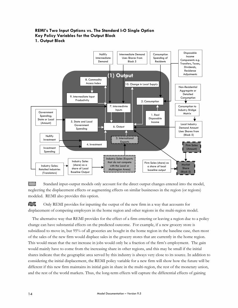
Model Documentation – Version 9.5 14
REMI’s Two Input Options vs. The Standard I-O Single Option Key Policy Variables for the Output Block 1. Output Block
8. Commodity Access Index 10. Change in Local Supply
1. Real Disposable
Income
2. Consumption
5. State and Local Government Spending
4. Investment
9. Intermediate Input Productivity
6. Output
7. Intermediate Inputs
Intermediate Demand Uses Shares from
Block 5
Consumption Spending of
Residents
Disposable Income
Components e.g. Transfers, Taxes,
Dividends, Residence
Adjustments
Local Industry Demand Amount Uses Shares from
(Block 5)
Firm Sales (Amount)
Market Share
(Block 5)
3. International Exports
Industry Sales (Exports that do not compete
with the Local or Multiregion Areas)
Industry Sales (share) as a
share of Local Baseline Output
Government Spending;
State or Local (Amount)
Nullify Investment
Investment Spending
Nullify Intermediate
Demand
Industry Sales: Retailed Industries
(Translators)
Non-Residential Aggregate or
Detailed Consumption
Consumption to Industry Bridge
Matrix
Firm Sales (share) as a share of local baseline output
(1) Output(1) Output
Standard input-output models only account for the direct output changes entered into the model,
neglecting the displacement effects or augmenting effects on similar businesses in the region (or regions) modeled. REMI also provides this option.
Only REMI provides for inputting the output of the new firm in a way that accounts for displacement of competing employers in the home region and other regions in the multi-region model.
The alternative way that REMI provides for the effect of a firm entering or leaving a region due to a policy change can have substantial effects on the predicted outcome. For example, if a new grocery store is subsidized to move in, but 95% of all groceries are bought in the home region in the baseline case, then most of the sales of the new firm would displace sales in the grocery stores that are currently in the home region. This would mean that the net increase in jobs would only be a fraction of the firm’s employment. The gain would mainly have to come from the increasing share in other regions, and this may be small if the initial shares indicate that the geographic area served by this industry is always very close to its source. In addition to considering the initial displacement, the REMI policy variable for a new firm will show how the future will be different if this new firm maintains its initial gain in share in the multi-region, the rest of the monetary union, and the rest of the world markets. Thus, the long-term effects will capture the differential effects of gaining

Model Documentation – Version 9.5 15
share in an industry in which demand in the relevant markets is expanding rapidly versus those in which the demand is growing slowly. It will also capture the way that future projected changes in output per worker will mean that sales growth and employment growth may differ markedly.
The range of other policy variables for the output block can be seen in the diagrams. These other ways that policy can influence the economic and demographic future of an area are not available for standard I-O models, because the linkages to most of the key processes that influence the outcomes in the region are not included in the structure of I-O models.
Block 2. Labor and Capital Demand
(2) Labor & Capital Demand(2) Labor & Capital Demand
Real Disposable
Income(Block 1)
Wage Rate vs. Capital (Block 4)
Output (Block 1)
Investment (Block 1)
Real Disposable Income
(Block 1)
Calculating Earnings(Block 1)
Composite Wage Rate
(Block 4)
8. Actual Capital Stock
3. OccupationEmployment
1. LaborProductivity
5. Factor Price Substitution
Effects
9. Gap between Actual and
Optimal Stock 7. Optimal Non-
Residential Capital Stock
4. Labor Access Index
by Occupation and Industry
6. Capital Intensity
10. Optimal Residential
Capital Stock
2. Industry Employment
The Labor and Capital Demand block includes employment, capital demand, labor productivity, and the
substitution among labor, capital, and fuel. Total employment is made up of farm, government, and private non-farm employment. Employment in private non-farm industries depends on employment demand and the number of workers needed to produce a unit of output. Employment demand is built up from the separate components of employment due to intermediate demand, consumer demand, local and regional government demand, local investment, and exports outside of the area. The employment per dollar of output depends on the national employment per dollar of output, the cost of other factors, and the access to specialized workers.
The availability of a large pool of workers within a region contributes to the labor force productivity. Each worker brings a set of unique characteristics and skills, even within the same occupational category. For

Model Documentation – Version 9.5 16
example, a surgeon may specialize in heart, brain, or knee surgery. Although a brain surgeon may be able to perform a heart operation, the brain surgeon is likely to be less effective than a surgeon who has specific experience with heart surgery. Hospitals in major medical centers such as Houston are in an excellent position to meet their staff requirements because the number of qualified job applicants in the region is so large.
More broadly, locations that can be easily reached by a large number of potential employees can better match jobs with workers. The equation for labor productivity due to labor access is calculated separately for each occupation. Occupational productivity in each location is based on the residential location of all potential workers and their actual or potential commuting costs to that location.
The contribution of labor variety to productivity is measured by an occupation-specific elasticity of substitution based on a study that considered wages and commuting patterns across a large metropolitan area. While the match of workers in specialized roles that are consistent with their training has a large impact on productivity for medical occupations, it is significantly less important for workers in the food service sector. Industry productivity due to specialization is built up from occupational productivity, using the proportionate number of workers in each occupation that are employed by a given industry.
The number of employees needed per unit of output depends on the use of other factors of production as well as labor access issues. Labor intensity, which measures the use of labor relative to other factors, is determined by the cost of labor relative to the cost of capital and fuel. The substitution between labor, capital, and fuel is based on a Cobb-Douglas production function, which implies constant factor shares. Labor intensity is calculated for each industry.
Demand for capital is driven by the optimal capital stock equation for industries and for housing. The optimal level of capital is determined for non-residential structures and equipment for each industry. The regional optimal capital stock is based on the industry size measured in capital-weighted employment terms, the cost of capital relative to labor, and a measure of the optimal capital stock on the national level. The variable for employment weighted by capital use is determined by the capital weight, employment, and labor productivity. The capital weight is the ratio of industry capital to employment in the region compared to the capital to employment ratio for the nation. The national optimal capital stock is based on the investment in the nation, the actual capital stock, the speed of adjustment, and the depreciation rate.
The optimal level of capital for residential housing is determined by the real disposable income in the region relative to the nation, the optimal residential capital stock for the nation, and the price of housing. To account for the cost of fuel, the fuel components of production (coal mining, petroleum refining, electric and natural gas utilities) are taken out of intermediate industry transactions and considered as a value-added factor of production. Then, firms substitute between labor, capital, and fuel (electric, natural gas, and residual fuel) as the relative costs of factor inputs change.

Model Documentation – Version 9.5 17
Block 3. Population and Labor Force
(3) Population Labor Supply(3) Population Labor Supply
1. Economic Migration
5. Participation Rate
4. The Employment to Potential Labor
Force 3. Potential Labor Force
2. Population
6. Labor Force
Local GovernmentSpending (Block 1)
Housing Price
(Block 4)
EmploymentOpportunity
(Block 4)
Compensation(Block 4)
Residence Adjusted
Employment (Block 2)
Relative Real Comp. Rate (Block
4)
Commodity AccessIndex
(Block 1)
EmploymentOpportunity
E/LF(Block 4)
Relative Real Comp.
Rate (Block 4)
The Population and Labor Force block includes detailed demographic information about the region. The
population is central to the regional economy, both as a source of demand for consumer and government spending and as the determinant of labor supply. As the composition of the population changes through births, deaths, and migration, so goes the region.
The demographic block is based on the cohort-survival method. Population in any given year is determined by adding the net natural change and the migration change to the previous year’s population. The natural change is caused by births and deaths, while migration occurs for economic and non-economic reasons. Population data is given for age, gender, and ethnic category.
Birth rates are the ratio of births to the number of women in each age group. The survival rate is equal to one minus the death rate, which is the ratio of deaths to population in each cohort. Since birth rates vary widely across age and ethnic groups, and survival rates vary widely for gender as well as age and ethnic category, the detailed demographic breakdown is needed to accurately capture the aggregate birth and survival rates.
Migration, economic or non-economic, also varies widely across population groups. Changes in retirement, international, and returning military migration are all assumed to occur for reasons that are not primarily due to with changing regional economic conditions. Retirement migration depends on the retirement-age population in the rest of the country for regions that have gained retirement population in the

Model Documentation – Version 9.5 18
past, and on the retirement-age population within the regions for places that tend to have a net loss of retirees. The probability of losing or gaining a retiree is age and gender specific for each age group.
International migration is also based on previous patterns. Changes in political restrictions on immigration and the economy of the immigrants’ country are more significant in determining international migration than are changes in the economy of the home region. Returning military migration patterns are also better explained by existing patterns than by regional economic conditions, so returning military is also an exogenous variable.
Economic migration is the movement of people to regions with better economic conditions. Economic migrants are attracted to places with relatively high wages and employment opportunities. Migrants are also attracted to places with high amenities. Potential migrants value access to consumer commodities, which depend on economic conditions. Thus, as the output of consumer goods and services increases, the amenity attraction of the region increases. Other amenities are due to non-economic factors. These amenities or compensating differentials are measured indirectly by looking at migration patterns over the last 20 years. In this way, the compensating differential is calculated as the expected wage rate that would result in no net in- or out-migration. For example, people may be willing to work in Florida even if paid only 85% of the average U.S. wage rate.
The labor force consists of unemployed individuals who are seeking work as well as employed workers. The labor force participation rate is thus the proportion of each population group that is working or looking for work. To predict the labor force, the model sums up the participation rate and cohort size for each demographic category. Participation rates vary widely across age, gender, and ethnic category; thus, the labor force depends in large part on the population structure of the region.
The willingness of individuals to participate in the labor force is also responsive to economic conditions. Higher wage rates and greater employment opportunities generally encourage higher labor force participation rates. The extent to which rates change in response to these economic factors, however, differs substantially for different population groups. For example, the willingness of men to enter the labor force is more influenced by wages, while women are more sensitive to employment opportunities.
Model Documentation – Version 9.5 19
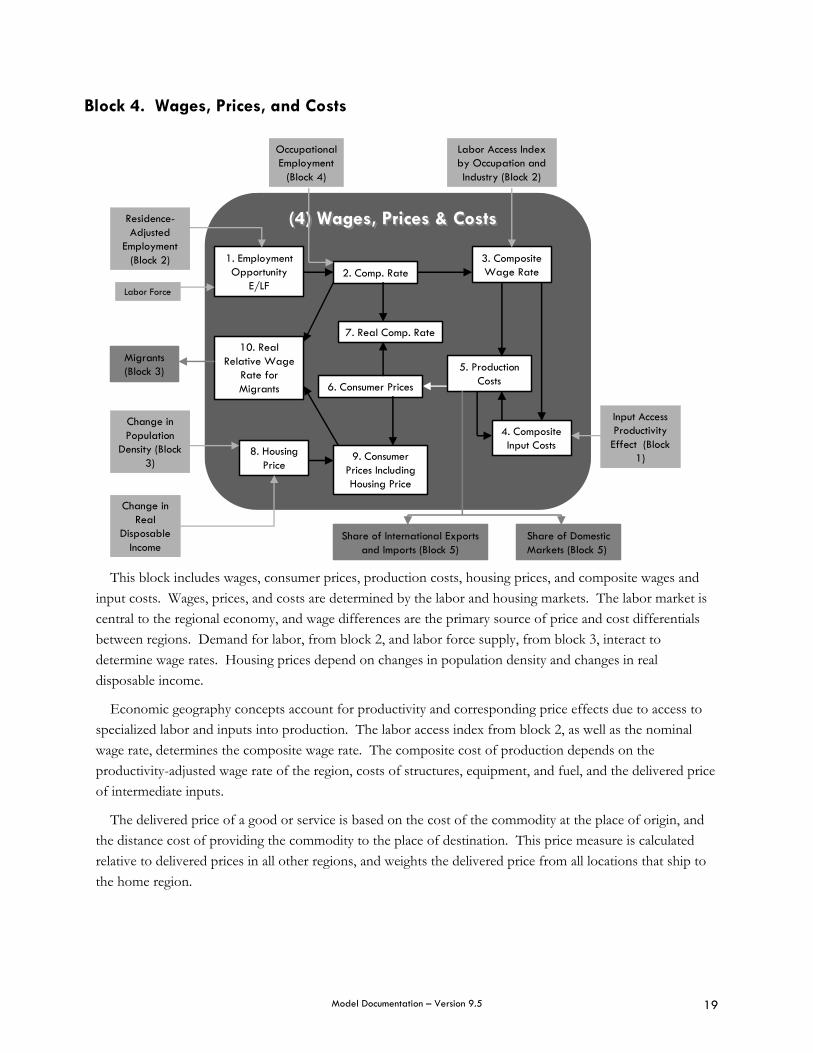
Block 4. Wages, Prices, and Costs
(4) Wages, Prices & Costs(4) Wages, Prices & Costs
1. Employment Opportunity
E/LF
8. Housing Price
10. Real Relative Wage
Rate for Migrants
9. Consumer Prices Including Housing Price
7. Real Comp. Rate
6. Consumer Prices
2. Comp. Rate3. Composite Wage Rate
4. Composite Input Costs
5. Production Costs
Migrants (Block 3)
Share of International Exports and Imports (Block 5)
Share of Domestic Markets (Block 5)
Labor Access Index by Occupation and Industry (Block 2)
Input Access Productivity Effect (Block
1)
Change in Population
Density (Block 3)
Change in Real
Disposable Income
Residence-Adjusted
Employment (Block 2)
Occupational Employment
(Block 4)
Labor Force
This block includes wages, consumer prices, production costs, housing prices, and composite wages and
input costs. Wages, prices, and costs are determined by the labor and housing markets. The labor market is central to the regional economy, and wage differences are the primary source of price and cost differentials between regions. Demand for labor, from block 2, and labor force supply, from block 3, interact to determine wage rates. Housing prices depend on changes in population density and changes in real disposable income.
Economic geography concepts account for productivity and corresponding price effects due to access to specialized labor and inputs into production. The labor access index from block 2, as well as the nominal wage rate, determines the composite wage rate. The composite cost of production depends on the productivity-adjusted wage rate of the region, costs of structures, equipment, and fuel, and the delivered price of intermediate inputs.
The delivered price of a good or service is based on the cost of the commodity at the place of origin, and the distance cost of providing the commodity to the place of destination. This price measure is calculated relative to delivered prices in all other regions, and weights the delivered price from all locations that ship to the home region.
Model Documentation – Version 9.5 20
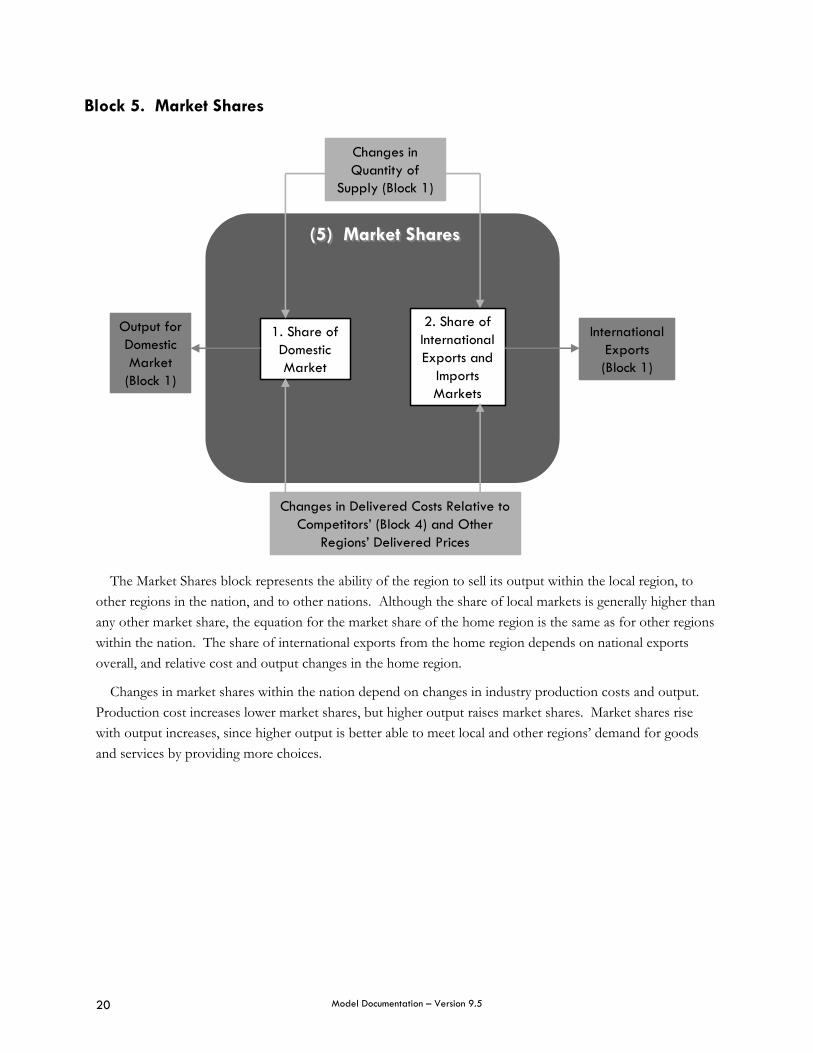
Block 5. Market Shares
(5) Market Shares(5) Market Shares
1. Share of Domestic Market
2. Share of International Exports and
Imports Markets
Output for Domestic Market (Block 1)
International Exports (Block 1)
Changes in Quantity of
Supply (Block 1)
Changes in Delivered Costs Relative to Competitors’ (Block 4) and Other
Regions’ Delivered Prices
The Market Shares block represents the ability of the region to sell its output within the local region, to
other regions in the nation, and to other nations. Although the share of local markets is generally higher than any other market share, the equation for the market share of the home region is the same as for other regions within the nation. The share of international exports from the home region depends on national exports overall, and relative cost and output changes in the home region.
Changes in market shares within the nation depend on changes in industry production costs and output. Production cost increases lower market shares, but higher output raises market shares. Market shares rise with output increases, since higher output is better able to meet local and other regions’ demand for goods and services by providing more choices.
Model Documentation – Version 9.5 21
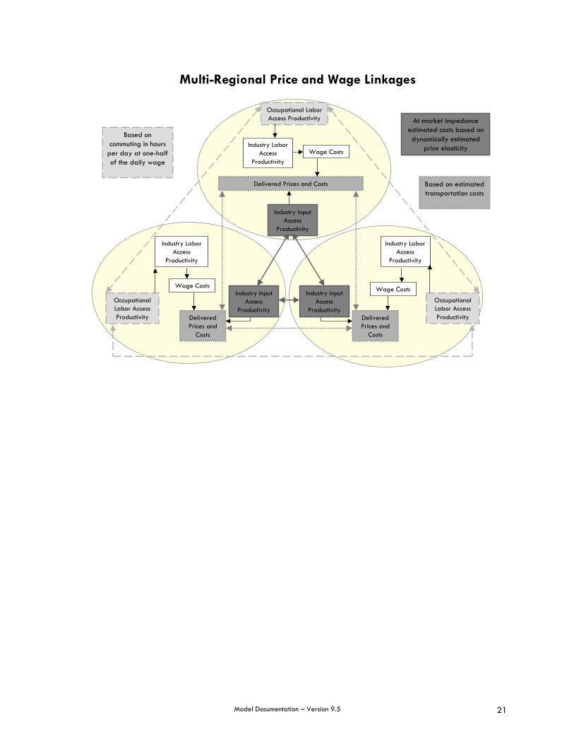
Multi-Regional Price and Wage Linkages
Industry Input Access
Productivity
Industry Input Access
Productivity
Industry Input Access
Productivity
At market impedanceestimated costs based on dynamically estimated
price elasticity
Occupational Labor Access Productivity
Occupational Labor Access Productivity
Occupational Labor Access Productivity
Based on commuting in hours
per day at one-half of the daily wage
Wage Costs
Industry Labor Access
Productivity
Wage Costs Industry Labor
Access Productivity
Wage Costs
Industry Labor Access
Productivity
Delivered Prices and Costs
Delivered Prices and
Costs
Delivered Prices and
Costs
Based on estimated transportation costs
Model Documentation – Version 9.5 22
IV. Block by Block Equations
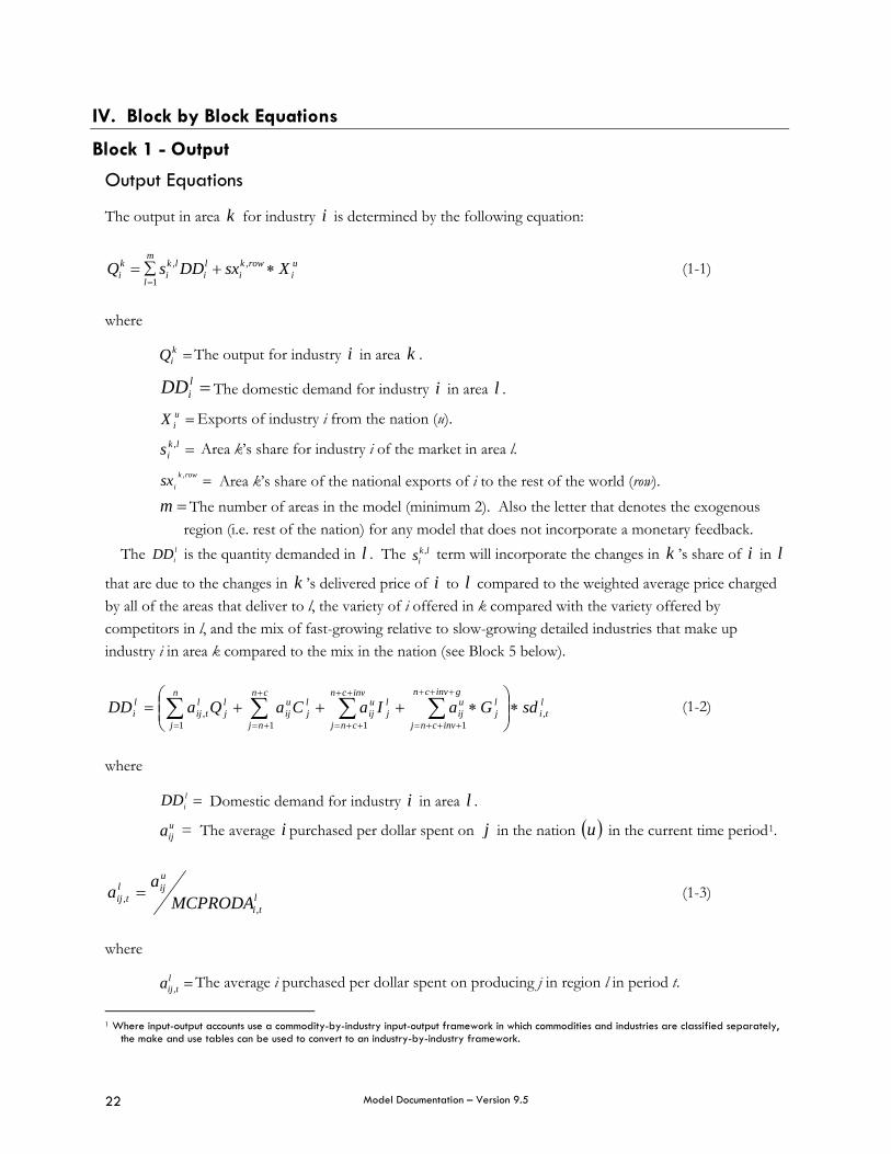
Block 1 - Output
Output Equations
The output in area k for industry i is determined by the following equation:
ui
rowki
li
lki
m
l
ki XsxDDsQ ∗+∑=
=
,,
1 (1-1)
where
=kiQ The output for industry i in area k .
=liDD The domestic demand for industry i in area l .
=uiX Exports of industry i from the nation (u).
=lkis , Area k’s share for industry i of the market in area l.
=rowkisx , Area k’s share of the national exports of i to the rest of the world (row). =m The number of areas in the model (minimum 2). Also the letter that denotes the exogenous region (i.e. rest of the nation) for any model that does not incorporate a monetary feedback.
The liDD is the quantity demanded in l . The lk
is , term will incorporate the changes in k ’s share of i in l
that are due to the changes in k ’s delivered price of i to l compared to the weighted average price charged by all of the areas that deliver to l, the variety of i offered in k compared with the variety offered by competitors in l, and the mix of fast-growing relative to slow-growing detailed industries that make up industry i in area k compared to the mix in the nation (see Block 5 below).
lti
lj
ginvcn
invcnj
uij
n
j
cn
nj
invcn
cnj
lj
uij
lj
uij
lj
ltij
li sdGaIaCaQaDD ,
11 1 1, ∗⎟⎟
⎠
⎞⎜⎜⎝
⎛∗+++= ∑∑ ∑ ∑
+++
+++==
+
+=
++
++=
(1-2)
where
=liDD Domestic demand for industry i in area l .
uija = The average i purchased per dollar spent on j in the nation ( )u in the current time period1.
lti
uijl
tij MCPRODAaa
,, = (1-3)
where
=ltija , The average i purchased per dollar spent on producing j in region l in period t.
1 Where input-output accounts use a commodity-by-industry input-output framework in which commodities and industries are classified separately,
the make and use tables can be used to convert to an industry-by-industry framework.
Model Documentation – Version 9.5 23
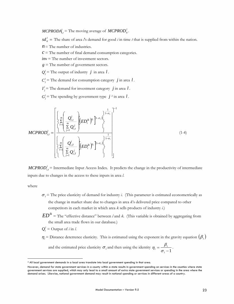
ltiMCPRODA , = The moving average of l
itMCPROD .
=litsd The share of area l’s demand for good i in time t that is supplied from within the nation.
n= The number of industries. c = The number of final demand consumption categories. inv = The number of investment sectors. g = The number of government sectors.
ljQ = The output of industry j in area l . ljC = The demand for consumption category j in area l .
ljI = The demand for investment category j in area l . ljG = The spending by government type j 2 in area l .
( )[ ]( )
( )[ ]( )
1
11
1
,1
,
1
11
1
,1
,
1
,
−
−
−
=
=
−
−
=
=
⎥⎥⎥⎥⎥⎥⎥⎥⎥⎥
⎦
⎤
⎢⎢⎢⎢⎢⎢⎢⎢⎢⎢
⎣
⎡
⎪⎭
⎪⎬
⎫
⎪⎩
⎪⎨
⎧
⎟⎟⎟⎟
⎠
⎞
⎜⎜⎜⎜
⎝
⎛
ΣΣ
⎪⎭
⎪⎬
⎫
⎪⎩
⎪⎨
⎧
⎟⎟⎟⎟
⎠
⎞
⎜⎜⎜⎜
⎝
⎛
ΣΣ
=i
ii
i
ii
lki
jTi
m
j
lTi
m
l
lki
jti
m
j
lti
m
l
lti
EDQ
Q
EDQ
Q
MCPRODσ
ση
σ
ση
(1-4)
ltiMCPROD , = Intermediate Input Access Index. It predicts the change in the productivity of intermediate
inputs due to changes in the access to these inputs in area l.
where
iσ = The price elasticity of demand for industry i. (This parameter is estimated econometrically as
the change in market share due to changes in area k’s delivered price compared to other competitors in each market in which area k sells products of industry i.) lkED = The “effective distance” between l and k. (This variable is obtained by aggregating from
the small area trade flows in our database.) liQ = Output of i in l.
iη = Distance deterrence elasticity. This is estimated using the exponent in the gravity equation ( )iβ
and the estimated price elasticity iσ and then using the identity 1−
=i
ii σ
βη .
2 All local government demands in a local area translate into local government spending in that area. However, demand for state government services in a county within a state results in government spending on services in the counties where state government services are supplied, which may only lead to a small amount of extra state government services or spending in the area where the demand arises. Likewise, national government demand may result in national spending or services in different areas of a country.
Model Documentation – Version 9.5 24
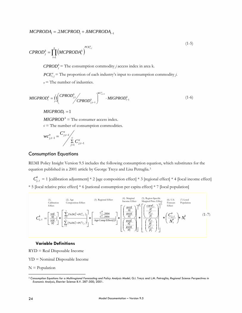
( )u
jiPCEn
i
ki
kj
ttt
MCPRODACPROD
MCPRODAMCPRODMCPRODA
,
1
18.2.
∏=
−
=
+=
(1-5)
kjCPROD = The consumption commodity j access index in area k.
ujiPCE , = The proportion of each industry’s input to consumption commodity j.
n = The number of industries.
kt
WC
ktj
ktj
c
j
kt MIGPRODCPROD
CPRODMIGPRODu
tj
11,
,
1
1,
−−=
⋅⎟⎟⎠
⎞⎜⎜⎝
⎛Π=
−
(1-6)
1=TMIGPROD kMIGPROD = The consumer access index.
c = The number of consumption commodities.
utj
c
j
utju
tjC
Cwc1,1
1,1,
−=
−−
Σ=
Consumption Equations
REMI Policy Insight Version 9.5 includes the following consumption equation, which substitutes for the equation published in a 2001 article by George Treyz and Lisa Petraglia.3
tjkC , = 1 [calibration adjustment] * 2 [age composition effect] * 3 [regional effect] * 4 [local income effect]
* 5 [local relative price effect] * 6 [national consumption per capita effect] * 7 [local population]
(1). Calibration Effect
(2). Age Composition Effect
(3). Regional Effect (4). Marginal Income Effect
(5). Region-Specific Marginal Price Effect (6). U.S.
Forecast Effect
( )
( )
j
Tu
Tu
Tk T
ktu
tu
tk
tk
jujR
tjT
utu
tjt
utk
TuTu
TkTk
NRYD
NRYD
NRYD
NRYD
CC
PCDG
PCDG
NYDN
YD
tjkC
β
⎥⎥⎥⎥⎥
⎦
⎤
⎢⎢⎢⎢⎢
⎣
⎡
⎟⎟⎠
⎞⎜⎜⎝
⎛
⎟⎟⎠
⎞⎜⎜⎝
⎛
∗⎥⎦
⎤⎢⎣
⎡∗
⎥⎥
⎦
⎤
⎢⎢
⎣
⎡
∑
∑∗⎥
⎦
⎤⎢⎣
⎡=
=
=
∗
∗
Effect(2) Comp Age2004,2004,
%
%
, 7
1,
7
1,
tk
tutj
u
PPP
PP
PP
CIFP
NN
C
J
TuTj
uTkTj
ktu
tjutk
tjk
∗⎟⎠⎞
⎜⎝⎛∗
⎥⎥⎥⎥⎥
⎦
⎤
⎢⎢⎢⎢⎢
⎣
⎡
⎟⎟⎠
⎞⎜⎜⎝
⎛
⎟⎟⎠
⎞⎜⎜⎝
⎛
∗ ,
,
,
,
,
γ(7) Local Population
Variable Definitions
RYD = Real Disposable Income
YD = Nominal Disposable Income
N = Population 3 Consumption Equations for a Multiregional Forecasting and Policy Analysis Model; G.I. Treyz and L.M. Petraglia; Regional Science Perspectives in
Economic Analysis, Elsevier Science B.V. 287-300; 2001.
(1-7)
Model Documentation – Version 9.5 25
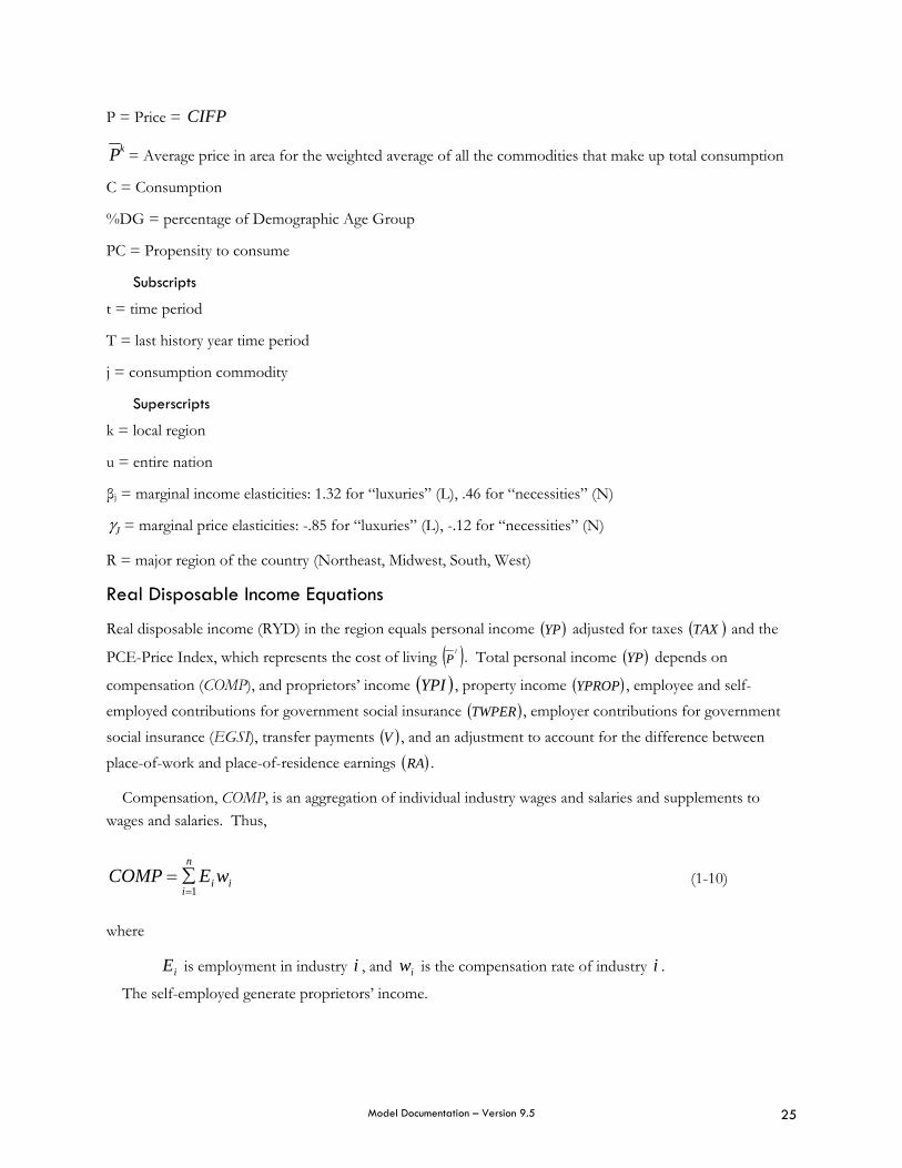
P = Price = CIFP
kP = Average price in area for the weighted average of all the commodities that make up total consumption
C = Consumption
%DG = percentage of Demographic Age Group
PC = Propensity to consume
Subscripts
t = time period
T = last history year time period
j = consumption commodity
Superscripts
k = local region
u = entire nation
βj = marginal income elasticities: 1.32 for “luxuries” (L), .46 for “necessities” (N)
Jγ = marginal price elasticities: -.85 for “luxuries” (L), -.12 for “necessities” (N)
R = major region of the country (Northeast, Midwest, South, West)
Real Disposable Income Equations
Real disposable income (RYD) in the region equals personal income ( )YP adjusted for taxes ( )TAX and the
PCE-Price Index, which represents the cost of living ( )lP . Total personal income ( )YP depends on
compensation (COMP), and proprietors’ income ( )YPI , property income ( )YPROP , employee and self-employed contributions for government social insurance ( )TWPER , employer contributions for government social insurance (EGSI), transfer payments ( )V , and an adjustment to account for the difference between place-of-work and place-of-residence earnings ( )RA .
Compensation, COMP, is an aggregation of individual industry wages and salaries and supplements to wages and salaries. Thus,
ii
n
iwECOMP
1=∑= (1-10)
where
iE is employment in industry i , and iw is the compensation rate of industry i .
The self-employed generate proprietors’ income.
Model Documentation – Version 9.5 26
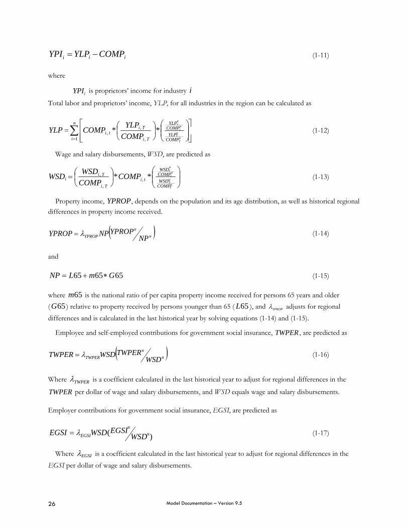
iii COMPYLPYPI −= (1-11)
where
iYPI is proprietors’ income for industry i
Total labor and proprietors’ income, YLP, for all industries in the region can be calculated as
YLP =∑= ⎥
⎥⎦
⎤
⎢⎢⎣
⎡⎟⎟⎠
⎞⎜⎜⎝
⎛⎟⎠⎞
⎜⎝⎛n
i COMPYLP
COMPYLP
Ti
Titi
TuT
utut
u
COMPYLPCOMP
1 ,
,, ** (1-12)
Wage and salary disbursements, WSD, are predicted as
⎟⎟⎠
⎞⎜⎜⎝
⎛⎟⎠⎞
⎜⎝⎛=
TuT
utut
u
COMPWSDCOMPWSD
tiTi
Tii COMP
COMPWSDWSD ** ,
,
, (1-13)
Property income, YPROP, depends on the population and its age distribution, as well as historical regional differences in property income received.
( )uu
YPROP NPYPROPNPYPROP λ= (1-14)
and
656565 GmLNP ∗+= (1-15)
where 65m is the national ratio of per capita property income received for persons 65 years and older ( 65G ) relative to property received by persons younger than 65 ( 65L ), and YPROPλ adjusts for regional differences and is calculated in the last historical year by solving equations (1-14) and (1-15).
Employee and self-employed contributions for government social insurance, TWPER , are predicted as
( )uu
TWPER WSDTWPERWSDTWPER λ= (1-16)
Where TWPERλ is a coefficient calculated in the last historical year to adjust for regional differences in the
TWPER per dollar of wage and salary disbursements, and WSD equals wage and salary disbursements.
Employer contributions for government social insurance, EGSI, are predicted as
)( uu
EGSI WSDEGSIWSDEGSI λ= (1-17)
Where EGSIλ is a coefficient calculated in the last historical year to adjust for regional differences in the EGSI per dollar of wage and salary disbursements.
Model Documentation – Version 9.5 27
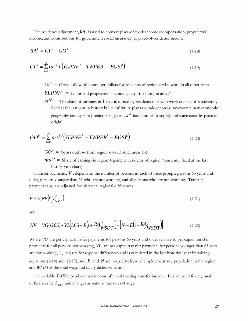
The residence adjustment, RA , is used to convert place-of-work income (compensation, proprietors’ income, and contributions for government social insurance) to place-of-residence income.
kkk GOGIRA −= (1-18)
( )lllkln
l
k EGSITWPERYLPNFrsGI −−∗∑==
,
1 (1-19)
=kGI Gross inflow of commuter dollars for residents of region k who work in all other areas.
=lYLPNF Labor and proprietors’ income (except for farm) in area l.
=klrs , The share of earnings in l that is earned by residents of k who work outside of k (currently fixed at the last year in history in lieu of future plans to endogenously incorporate new economic
geography concepts to predict changes in lkrs based on labor supply and wage costs by place of origin).
( )kkklkm
kl
k EGSITWPERYLPNFnrsGO −−∑=≠
, (1-20)
=kGO Gross outflow from region k to all other areas (m).
=lknrs , Share of earnings in region k going to residents of region l (currently fixed at the last history year share).
Transfer payments, V , depend on the number of persons in each of three groups: persons 65 years and older, persons younger than 65 who are not working, and all persons who are not working. Transfer payments also are adjusted for historical regional differences.
( )u
u
V NVVNVV λ= (1-21)
and
( ) ( )[ ] ( )[ ]WSDTRAENWSDT
RAELVLGVGNV +−++−+= 116565 (1-22)
Where VG are per capita transfer payments for persons 65 years and older relative to per capita transfer payments for all persons not working, VL are per capita transfer payments for persons younger than 65 who are not working, Vλ adjusts for regional differences and is calculated in the last historical year by solving
equations (1-16) and (1-17), and E and N are, respectively, total employment and population in the region and WSDT is the total wage and salary disbursements.
The variable TAX depends on net income after subtracting transfer income. It is adjusted for regional differences by TAXλ and changes as national tax rates change.
Model Documentation – Version 9.5 28
( ) ( )⎥⎦⎤
⎢⎣⎡
−−= uu
u
TAX VYPTAXVYPTAX λ (1-23)
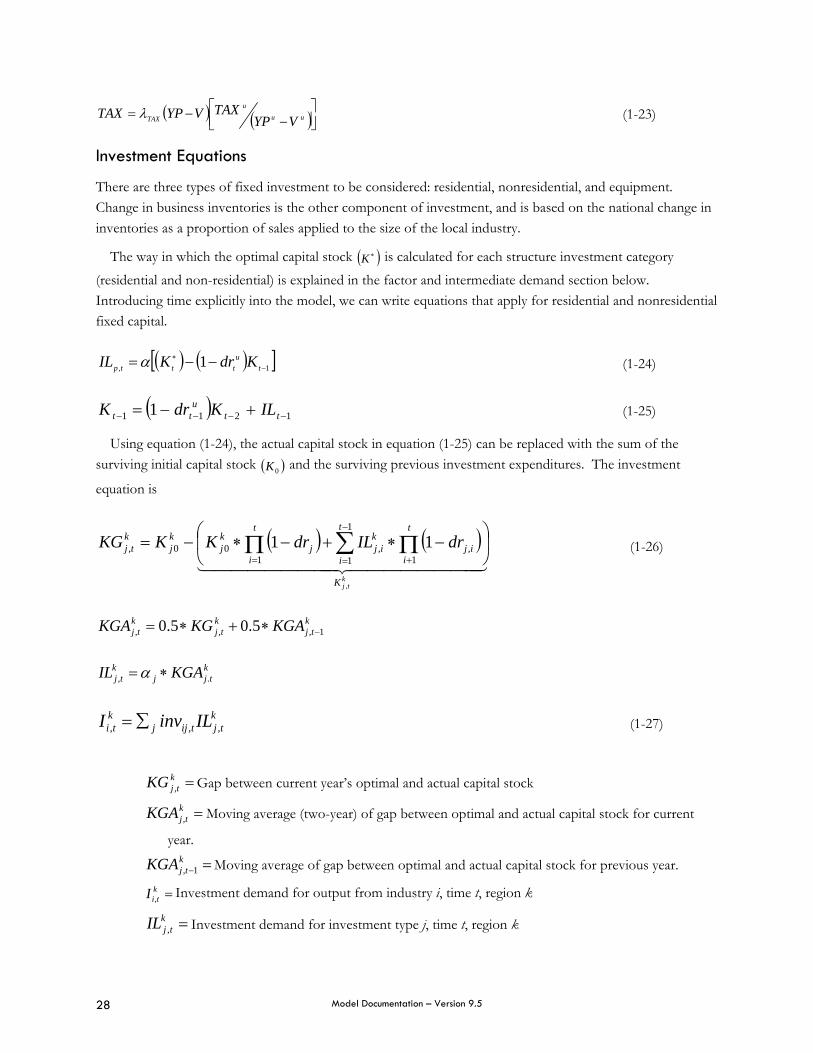
Investment Equations
There are three types of fixed investment to be considered: residential, nonresidential, and equipment. Change in business inventories is the other component of investment, and is based on the national change in inventories as a proportion of sales applied to the size of the local industry.
The way in which the optimal capital stock ( )∗K is calculated for each structure investment category (residential and non-residential) is explained in the factor and intermediate demand section below. Introducing time explicitly into the model, we can write equations that apply for residential and nonresidential fixed capital.
( ) ( )[ ]1, 1 −∗ −−= t
utttp KdrKIL α (1-24)
( ) 1211 1 −−−− +−= ttu
tt ILKdrK (1-25)
Using equation (1-24), the actual capital stock in equation (1-25) can be replaced with the sum of the surviving initial capital stock ( )0K and the surviving previous investment expenditures. The investment
equation is
( ) ( )44444444 344444444 21
ktjK
t
iij
t
i
kijj
t
i
kj
kj
ktj drILdrKKKG
,
1
1,
1,
100, 11 ⎟
⎠
⎞⎜⎝
⎛−∗+−∗−= ∑ ΠΠ
−
= += (1-26)
ktj
ktj
ktj KGAKGKGA 1,,, 5.05.0 −∗+∗=
ktjj
ktj KGAIL ., ∗= α
ktjtijj
kti ILinvI ,,, ∑= (1-27)
=ktjKG , Gap between current year’s optimal and actual capital stock
=ktjKGA , Moving average (two-year) of gap between optimal and actual capital stock for current
year.
=−k
tjKGA 1, Moving average of gap between optimal and actual capital stock for previous year.
=ktiI , Investment demand for output from industry i, time t, region k
=ktjIL , Investment demand for investment type j, time t, region k
Model Documentation – Version 9.5 29
=tijinv , Coefficient denoting the proportion of investment category j supplied by industry i, time t.
=*,
ktjK Optimal capital stock, type j, time t, region k.
=kjK 0 Capital stock, type j, time 0, region k.
=jdr Depreciation rate, type j.
=jα Speed of adjustment, type j.
(For additional details see Rickman, Shao and Treyz, 1993).
Producers’ durable equipment investment is calculated somewhat differently from residential and nonresidential investment. Since a very large part of equipment investment is for replacement, and not net new purchases, the following equation is used:
))/((86.0))/((14.0 ,,,,,,,u
tPDEu
tNRSk
tNRSu
tPDEu
tNRSk
tNRSk
tPDE ILKKILILILIL ∗∗+∗∗= (1-28)
=ktPDEIL , Investment demand for producers’ durable equipment, time t, region k.
=ktNRSIL , Investment demand for nonresidential, time t, region k.
=utNRSIL , Investment demand for nonresidential, time t, national (u).
=utPDEIL , Investment demand for producers’ durable equipment, time t, national (u).
=ktNRSK , Capital stock for nonresidential, time t, region k.
=utNRSK , Capital stock for nonresidential, time t, national (u).
The national change in business inventories is allocated according to the regional share of employment.
uiu
i
lil
i CBIEECBI ∗⎟
⎠⎞
⎜⎝⎛= (1-29)
=liCBI The change in business inventories, industry i, region l.
=uiCBI The change in business inventories, industry i, national (u).
=liE Employment, industry i, region l.
=uiE Employment, industry i, national (u).
Government Spending Equations
The state and local government demand equations are driven based on the average per capita demand for these services in the last history year (T).
Model Documentation – Version 9.5 30
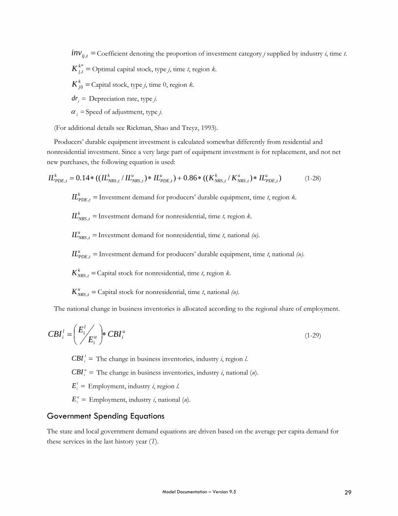
⎟⎟⎠
⎞⎜⎜⎝
⎛÷∗∗= u
T
uTstate
ut
utstatel
tlstate
ltstate N
GN
GNG ,,
, λ (1-30)
⎟⎟⎠
⎞⎜⎜⎝
⎛÷∗∗= u
T
uTlocal
ut
utlocall
tllocal
ltlocal N
GN
GNG ,,
, λ (1-31)
where
=ltstateG , The demand for state services in region l, time t.
=ltlocalG , The demand for local services in region l, time t.
=llocalλ An estimate of the last history year local government spending per capita in region l.
=lstateλ An estimate of the state last history year average spending per capita in the state in region l.
=ltN The total population, region l, time t.
Superscript u indicates similar values for the nation.
In the absence of adequate local demand estimates for state and local government separately, it is necessary to approximate these relative values based on assuming uniform productivity across all state and local government employees in the nation. It is important to note that local demand for local government services will be met in the local area, whereas the demand for state services in a local area may be met in part by state employees in the counties that provide state services, as set forth in the section on Market Shares below.
Block 2 – Labor and Capital Demand
Labor Demand Equations
The productivity of labor depends on access to a labor pool. In this instance, we have chosen to use employment by occupation as the measure of access to the specialized labor pool. Thus, the variety effect on the productivity of labor by occupation is expressed in the following equation:
( )
( ) ii
jj
kluti
lti
m
l
kti
klu
tj
ltj
m
l
kj,t
ccEE
RCW
ccEOEO
FLO
σσ
σσ
−−
=
−−
=
⎥⎥⎦
⎤
⎢⎢⎣
⎡+∗Σ÷=
⎥⎥⎦
⎤
⎢⎢⎣
⎡+∗∑÷=
11
1,
,
,
1,
11
1,
,
,
1
11
11 (2-1a)
(2-1b)
=ktjFLO , Labor productivity for occupation type j that depends on the relative access to labor in
occupation j in region k, time t.
=ktiRCW , Relative labor productivity due to industry concentration of labor.

Model Documentation – Version 9.5 31
=ltjEO , Labor of occupation type j in region l, time t.
=jσ Elasticity of substitution (i.e. cost elasticity).
=klcc , Commuting time and expenses from l to k as a proportion of the wage rate.
=utjEO , Labor of occupation type j, national (u), time t.
=ltiE , Employment in industry i, time t, in region l.
=m Number of regions in model including the rest of the nation region.
The value of lσ is .12 and is based on elasticity estimates made by REMI under a grant from the National Cooperative Highway Research Program (Weisbrod, Vary, and Treyz, 2001) based on cross-commuting among workers in the same occupation observed in 1300 Traffic Analysis Zones in Chicago. Key data inputs on travel times were provided by Cambridge Systematics, Inc.
In order to determine labor productivity changes by industry due to access to variety, a staffing pattern matrix is used as follows:
kTi
kti
ktjij
q
j
kti FLRCWFLOdFl ,,,,
1, 2 ÷⎥
⎦
⎤⎢⎣
⎡÷⎥
⎦
⎤⎢⎣
⎡+⎟
⎠⎞
⎜⎝⎛ ∗∑=
= (2-1c)
=ktiFl , Labor productivity due to labor access to industry and relevant occupations by industry i, in
region k, time t, normalized by kTiFl ,
=ijd , Occupation j’s proportion of industry i’s employment.
=ktjFLO , The labor productivity for occupation j, region k, time t.
=q The number of occupations in industry i.
=kTiFL , Labor productivity due to access by industry i in region k in the last year of history.
=ktiRCW , Relative labor productivity due to industry concentration of labor.
Relative labor intensity is determined by the following equation based on Cobb-Douglas technology and the assumption that the optimal labor intensity is chosen when new equipment is installed.
( ) ( ) ( )⎥⎥⎥
⎦
⎤
⎢⎢⎢
⎣
⎡−∗+= −
−
−k
ti
h
bkti
bkti
bktik
tnrs
ktnrsk
tik
ti LRFCRCCRLCKI
LLkti
tjitjitji
1,,,1
,,
,1,,
,
,,,
444444 3444444 21 (2-2)
ktiL , = Relative labor intensity, industry i, time t, region k.
=tjib , Contribution to value added of factor j, (labor, capital, and fuel respectively), industry i, time t,
region k.
=ktnrsI , Nonresidential investment, region K, time t.
Model Documentation – Version 9.5 32
=ktnrsK , Nonresidential capital stock, region K, time t.
=ktiRCC , Relative capital cost, industry i, time t, region k.
ktiRLC , = Relative labor cost, industry i, time t, region k equals ⎟⎟
⎠
⎞⎜⎜⎝
⎛u
ti
kti
ww
,
, , before accounting for
labor productivity effects. ktiRFC , = Relative fuel cost industry i, time t, region k.
ktih , = Optimal labor intensity, industry i, time t, region k.
Simplified, the above equation can be written as,
( )kti
ktik
tnrs
ktnrsk
tik
ti LhKI
LL 1,,,
,1,, −− −∗⎟
⎟⎠
⎞⎜⎜⎝
⎛+= (2-3)
where
tiktiu
TiuTi
uti
uti
kTi
kTi
kTi
ktik
ti epvindxFlQEQE
QE
LL
EPV i,,
,,
,,
,
,
,
,, )( ∗∗⎟
⎟⎠
⎞⎜⎜⎝
⎛∗∗= −α (2-4)
ktiEPV , = Employees per dollar of output in industry i, time t, region k.
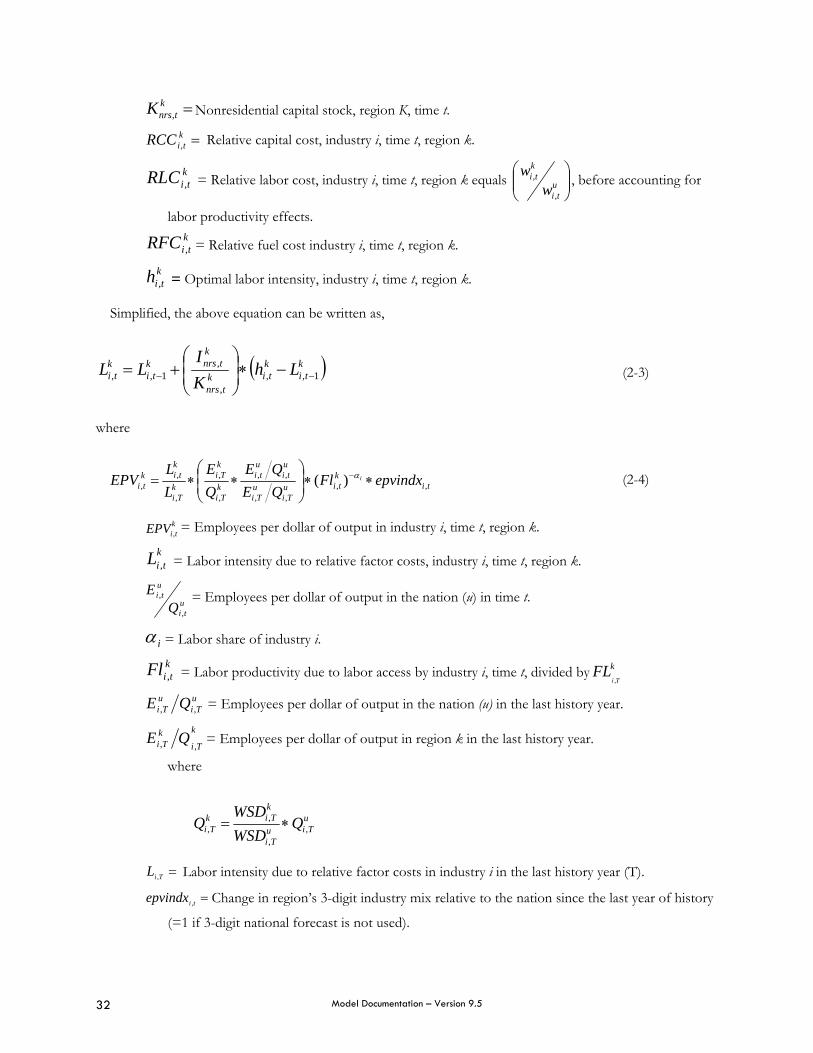
ktiL , = Labor intensity due to relative factor costs, industry i, time t, region k.
uti
uti
QE
,
, = Employees per dollar of output in the nation (u) in time t.
iα = Labor share of industry i. ktiFl , = Labor productivity due to labor access by industry i, time t, divided by k
TiFL
,
uTi
uTi QE ,, = Employees per dollar of output in the nation (u) in the last history year.
k
TikTi QE
,, = Employees per dollar of output in region k in the last history year.
where
uTiu
Ti
kTik
Ti QWSDWSD
Q ,,
,, ∗=
=TiL , Labor intensity due to relative factor costs in industry i in the last history year (T).
=tiepvindx , Change in region’s 3-digit industry mix relative to the nation since the last year of history
(=1 if 3-digit national forecast is not used).
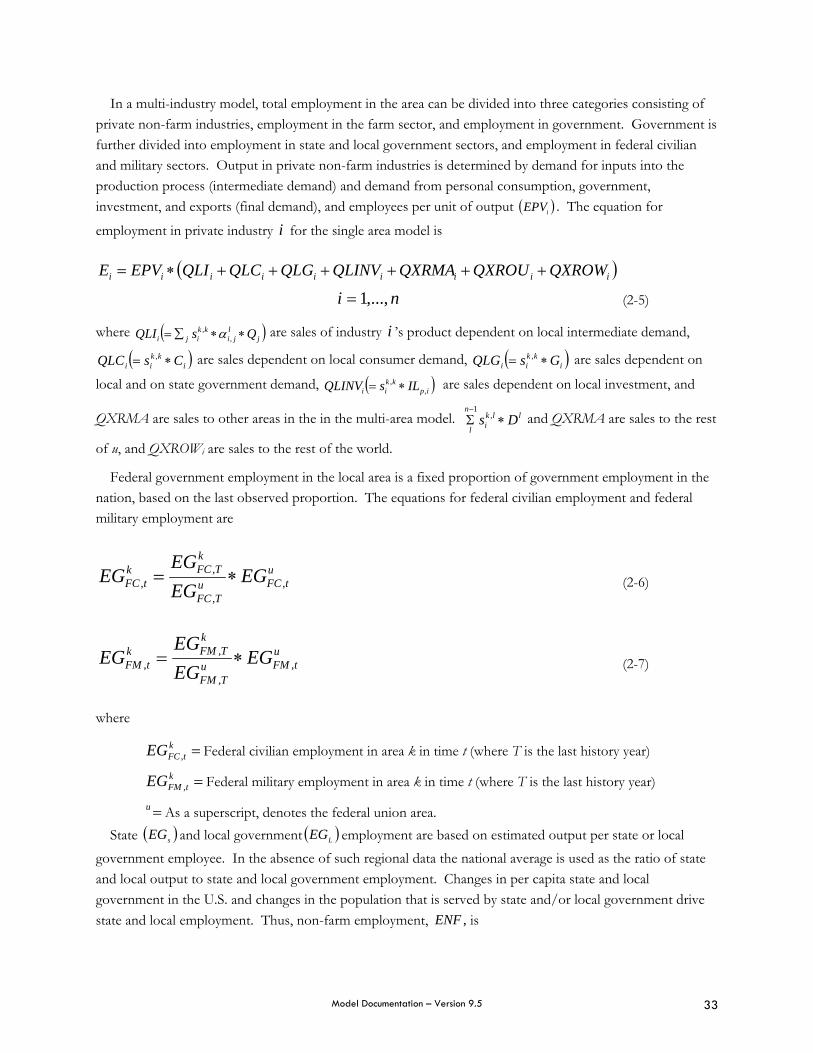
Model Documentation – Version 9.5 33
In a multi-industry model, total employment in the area can be divided into three categories consisting of private non-farm industries, employment in the farm sector, and employment in government. Government is further divided into employment in state and local government sectors, and employment in federal civilian and military sectors. Output in private non-farm industries is determined by demand for inputs into the production process (intermediate demand) and demand from personal consumption, government, investment, and exports (final demand), and employees per unit of output ( )iEPV . The equation for
employment in private industry i for the single area model is
( )iiiiiiiii QXROWQXROUQXRMAQLINVQLGQLCQLIEPVE ++++++∗=
ni ,...,1= (2-5)
where ( )jl
jikk
iji QsQLI ∗∗∑= ,, α are sales of industry i ’s product dependent on local intermediate demand,
( )ikk
ii CsQLC ∗= , are sales dependent on local consumer demand, ( )ikk
ii GsQLG ∗= , are sales dependent on
local and on state government demand, ( )ipkk
ii ILsQLINV ,, ∗= are sales dependent on local investment, and
QXRMA are sales to other areas in the in the multi-area model. llki
n
lDs ∗Σ
−,
1 and QXRMA are sales to the rest
of u, and QXROWi are sales to the rest of the world.
Federal government employment in the local area is a fixed proportion of government employment in the nation, based on the last observed proportion. The equations for federal civilian employment and federal military employment are
utFCu
TFC
kTFCk
tFC EGEGEG
EG ,,
,, ∗= (2-6)
utFMu
TFM
kTFMk
tFM EGEGEG
EG ,,
,, ∗= (2-7)
where
=ktFCEG , Federal civilian employment in area k in time t (where T is the last history year)
=ktFMEG , Federal military employment in area k in time t (where T is the last history year)
=u As a superscript, denotes the federal union area. State ( )sEG and local government ( )LEG employment are based on estimated output per state or local
government employee. In the absence of such regional data the national average is used as the ratio of state and local output to state and local government employment. Changes in per capita state and local government in the U.S. and changes in the population that is served by state and/or local government drive state and local employment. Thus, non-farm employment, ,ENF is
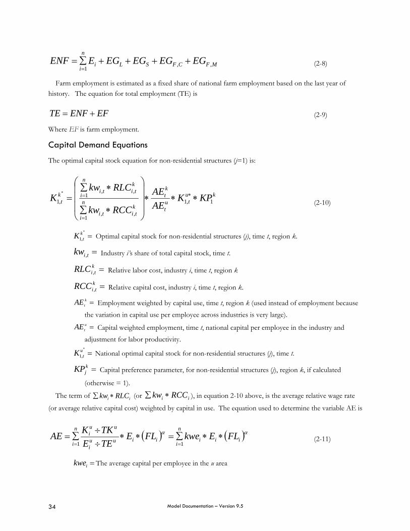
Model Documentation – Version 9.5 34
MFCFSLi
n
iEGEGEGEGEENF ,,
1++++∑=
= (2-8)
Farm employment is estimated as a fixed share of national farm employment based on the last year of history. The equation for total employment (TE) is
EFENFTE += (2-9)
Where EF is farm employment.
Capital Demand Equations
The optimal capital stock equation for non-residential structures (j=1) is:
kutu
t
kt
ktiti
n
i
ktiti
n
ikt KPK
AEAE
RCCkw
RLCkwK 1,1
,,1
,,1
,1
*
∗∗∗⎟⎟⎟
⎠
⎞
⎜⎜⎜
⎝
⎛
∗∑
∗∑= ∗
=
= (2-10)
=*
,1ktK Optimal capital stock for non-residential structures (j), time t, region k.
=tikw , Industry i’s share of total capital stock, time t.
=ktiRLC , Relative labor cost, industry i, time t, region k
=ktiRCC , Relative capital cost, industry i, time t, region k.
=ktAE Employment weighted by capital use, time t, region k (used instead of employment because the variation in capital use per employee across industries is very large).
=utAE Capital weighted employment, time t, national capital per employee in the industry and adjustment for labor productivity.
=*
,1utK National optimal capital stock for non-residential structures (j), time t.
=kjKP Capital preference parameter, for non-residential structures (j), region k, if calculated
(otherwise = 1).
The term of ii RLCkw ∗∑ (or ii RCCkw ∗∑ ), in equation 2-10 above, is the average relative wage rate
(or average relative capital cost) weighted by capital in use. The equation used to determine the variable AE is
( ) ( )ααiii
n
iiiuu
i
uui
n
iFLEkweFLE
TEETKKAE ∗∗∑=∗∗
÷÷
∑=== 11
(2-11)
=ikwe The average capital per employee in the u area
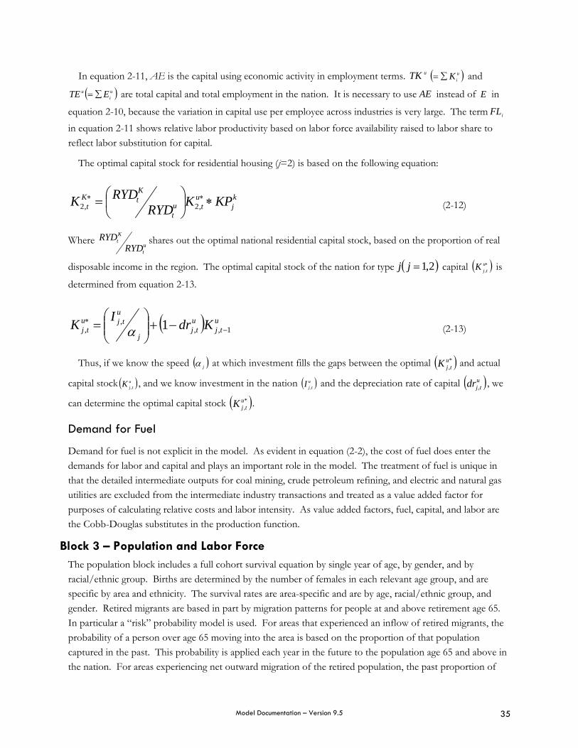
Model Documentation – Version 9.5 35
In equation 2-11, AE is the capital using economic activity in employment terms. uTK ( )uiK∑= and
( )ui
u ETE ∑= are total capital and total employment in the nation. It is necessary to use AE instead of E in
equation 2-10, because the variation in capital use per employee across industries is very large. The term iFL in equation 2-11 shows relative labor productivity based on labor force availability raised to labor share to reflect labor substitution for capital.
The optimal capital stock for residential housing (j=2) is based on the following equation:
kj
utu
t
KtK
t KPKRYDRYDK ∗⎟
⎠⎞
⎜⎝⎛= ∗∗
,2,2 (2-12)
Where ut
Kt
RYDRYD shares out the optimal national residential capital stock, based on the proportion of real
disposable income in the region. The optimal capital stock of the nation for type ( )2,1=jj capital ( )∗utjK , is
determined from equation 2-13.
( ) utj
utj
j
utju
tj KdrIK 1,,,
, 1 −∗ −+⎟⎟
⎠
⎞⎜⎜⎝
⎛= α (2-13)
Thus, if we know the speed ( )jα at which investment fills the gaps between the optimal ( )*,
utjK and actual
capital stock ( )utjK , , and we know investment in the nation ( )u
tjI , and the depreciation rate of capital ( )utjdr , , we
can determine the optimal capital stock ( )*,
utjK .
Demand for Fuel
Demand for fuel is not explicit in the model. As evident in equation (2-2), the cost of fuel does enter the demands for labor and capital and plays an important role in the model. The treatment of fuel is unique in that the detailed intermediate outputs for coal mining, crude petroleum refining, and electric and natural gas utilities are excluded from the intermediate industry transactions and treated as a value added factor for purposes of calculating relative costs and labor intensity. As value added factors, fuel, capital, and labor are the Cobb-Douglas substitutes in the production function.
Block 3 – Population and Labor Force The population block includes a full cohort survival equation by single year of age, by gender, and by racial/ethnic group. Births are determined by the number of females in each relevant age group, and are specific by area and ethnicity. The survival rates are area-specific and are by age, racial/ethnic group, and gender. Retired migrants are based in part by migration patterns for people at and above retirement age 65. In particular a “risk” probability model is used. For areas that experienced an inflow of retired migrants, the probability of a person over age 65 moving into the area is based on the proportion of that population captured in the past. This probability is applied each year in the future to the population age 65 and above in the nation. For areas experiencing net outward migration of the retired population, the past proportion of

Model Documentation – Version 9.5 36
loss is applied to the number of people in the local area that are age 65 and older. When the data supports it, the above-65 population can be divided into gender and age categories.
In particular, the equation for retired migrants is
( )( )uii
lii
li
li NRTDUMNRTDUMrmRTMG ∗+∗−= 1 (3-1)
where
=liRTMG The net inflow or outflow of migrants of age i (i=65,66, …100+) to region l
=lirm The net proportion of the relevant population that has historically migrated into or out of area l.
=liN The 65 and above population in area l.
=uiN The 65 and above population in area u.
=iRTDUM {
The economic migration equation in the model is very important to forecasting the effects of alternative policies. It is based on the assumption that economic migrants will make their migration decisions based on the relative expected after-tax real expected earned income in alternative locations and the relative amenity attractiveness of these locations.
The migration equation is
( ) ( ) ( )[ ] lt
lt
lt
lt
llt LFMIGPRODRWRREOECMG 1lnlnln −∗+++= βββλ (3-2)
where
=ltECMG Net economic migrants (all migrants less than 65 years of age) in area l.
=−l
tLF 1 The labor force last period in area l.
ut
ut
lt
lt
lt
LFE
LFE
REO =
=ltE Residence-adjusted employment in area l in period t.
=ltMIGPROD The consumption access index in area l in period t.
1 if 0>lirm
0 if 0<lirm
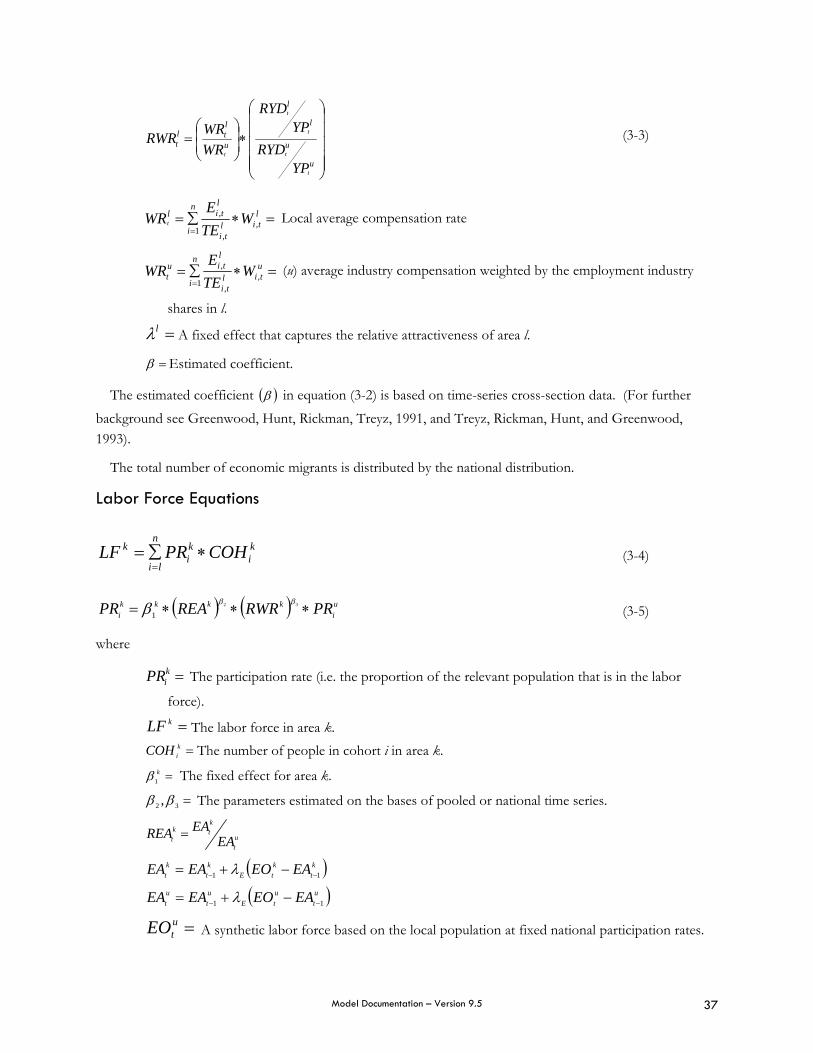
Model Documentation – Version 9.5 37
⎟⎟⎟⎟⎟
⎠
⎞
⎜⎜⎜⎜⎜
⎝
⎛
∗⎟⎟⎠
⎞⎜⎜⎝
⎛=
u
u
l
l
u
ltl
t
t
t
t
t
t
YPRYD
YPRYD
WRWRRWR (3-3)
=∗∑==
ltil
ti
lti
n
i
l WTEE
WRt ,,
,
1 Local average compensation rate
=∗∑==
util
ti
lti
n
i
ut W
TEE
WR ,,
,
1 (u) average industry compensation weighted by the employment industry
shares in l.
=lλ A fixed effect that captures the relative attractiveness of area l.
=β Estimated coefficient.
The estimated coefficient ( )β in equation (3-2) is based on time-series cross-section data. (For further background see Greenwood, Hunt, Rickman, Treyz, 1991, and Treyz, Rickman, Hunt, and Greenwood, 1993).
The total number of economic migrants is distributed by the national distribution.
Labor Force Equations
ki
ki
n
li
k COHPRLF ∗∑==
(3-4)
( ) ( ) ui
kkkki PRRWRREAPR ∗∗∗= 32
1
βββ (3-5)
where
=kiPR The participation rate (i.e. the proportion of the relevant population that is in the labor
force).
=kLF The labor force in area k. =k
iCOH The number of people in cohort i in area k.
=k1β The fixed effect for area k.
=32 , ββ The parameters estimated on the bases of pooled or national time series.
ut
ktk
t EAEAREA =
( )kt
ktE
kt
kt EAEOEAEA 11 −− −+= λ
( )ut
utE
ut
ut EAEOEAEA 11 −− −+= λ
=utEO A synthetic labor force based on the local population at fixed national participation rates.
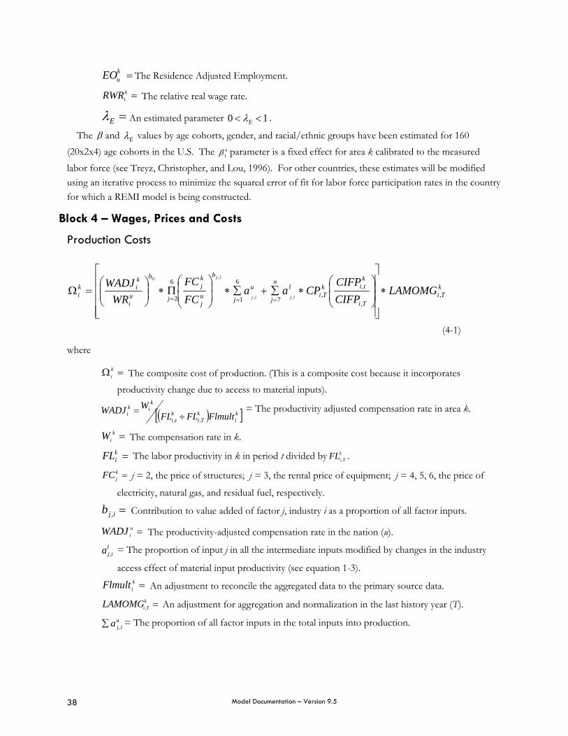
Model Documentation – Version 9.5 38
=ukEO The Residence Adjusted Employment.
=kiRWR The relative real wage rate.
=Eλ An estimated parameter 10 << Eλ .
The β and Eλ values by age cohorts, gender, and racial/ethnic groups have been estimated for 160 (20x2x4) age cohorts in the U.S. The k
1β parameter is a fixed effect for area k calibrated to the measured labor force (see Treyz, Christopher, and Lou, 1996). For other countries, these estimates will be modified using an iterative process to minimize the squared error of fit for labor force participation rates in the country for which a REMI model is being constructed.
Block 4 – Wages, Prices and Costs
Production Costs
kTi
Ti
ktik
Til
n
j
u
j
b
uj
kj
j
b
ui
kik
i LAMOMGCIFPCIFP
CPaaFCFC
WRWADJ
ijij
iji
,,
,,
7
6
1
6
2 ,,
,1
∗
⎥⎥⎥⎥
⎦
⎤
⎢⎢⎢⎢
⎣
⎡
⎟⎟⎠
⎞⎜⎜⎝
⎛∗∑+∑∗⎟
⎟⎠
⎞⎜⎜⎝
⎛Π∗⎟⎟
⎠
⎞⎜⎜⎝
⎛=Ω
===
(4-1)
where
=Ω ki The composite cost of production. (This is a composite cost because it incorporates
productivity change due to access to material inputs).
( )[ ]ki
kTi
kti
kik
i FlmultFLFLWWADJ
,, ÷= = The productivity adjusted compensation rate in area k.
=kiW The compensation rate in k.
=kiFL The labor productivity in k in period t divided by k
TiFL , .
=kjFC j = 2, the price of structures; j = 3, the rental price of equipment; j = 4, 5, 6, the price of
electricity, natural gas, and residual fuel, respectively.
=ijb , Contribution to value added of factor j, industry i as a proportion of all factor inputs.
=uiWADJ The productivity-adjusted compensation rate in the nation (u).
lija , = The proportion of input j in all the intermediate inputs modified by changes in the industry
access effect of material input productivity (see equation 1-3).
=kiFlmult An adjustment to reconcile the aggregated data to the primary source data.
=kTiLAMOMG , An adjustment for aggregation and normalization in the last history year (T).
uija ,∑ = The proportion of all factor inputs in the total inputs into production.
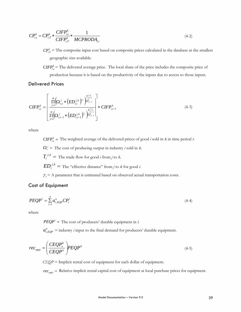
Model Documentation – Version 9.5 39
tikTi
ktik
Tikti MCPRODACIFP
CIFPCPCP
,,
,,,
1∗∗= (4-2)
kTiCP , = The composite input cost based on composite prices calculated in the database at the smallest
geographic size available.
ktiCIFP , = The delivered average price. The local share of the price includes the composite price of
production because it is based on the productivity of the inputs due to access to those inputs.
Delivered Prices
( )( )( )( )
kti
D
Tkj
tijti
m
j
D
Tkj
tijti
m
jkti CIFP
ED
EDCIFP
kti
kjti
i
kti
kjti
i
1,
,1,1,1
,,,1
,
1,
,1,
1,
,1,
−
−−=
= ∗
⎥⎥⎥⎥
⎦
⎤
⎢⎢⎢⎢
⎣
⎡
∗ΩΠ
∗ΩΠ=
−
−
−
−
γ
γ
(4-3)
where
=ktiCIFP , The weighted average of the delivered prices of good i sold in k in time period t.
=Ω ji The cost of producing output in industry i sold in k.
=kjiT , The trade flow for good i from j to k.
=kjiED , The “effective distance” from j to k for good i.
iγ = A parameter that is estimated based on observed actual transportation costs.
Cost of Equipment
li
uEQPi
n
i
l CPaPEQP ,1=
∑= (4-4)
where
=lPEQP The cost of producers’ durable equipment in l. u
EQPia , = industry i input to the final demand for producers’ durable equipment.
ku
kx
equi PEQPCEQPCEQP
rec ⎟⎟⎠
⎞⎜⎜⎝
⎛= (4-5)
CEQP = Implicit rental cost of equipment for each dollar of equipment.
=equirec Relative implicit rental capital cost of equipment at local purchase prices for equipment.

Model Documentation – Version 9.5 40
Consumption Deflator
For consumption category j in time t we assume Cobb-Douglas substitutability of the sectors that are inputs into this consumption commodity.
jiPCEti
i
utj
ltj CIFPCIFPCIFP ,
,,, ∏∗= (4-6)
where
=jiPCE , The proportion of commodity j obtained from industry i.
=ltjCIFP , The delivered (CIF) consumer price of consumption commodity j in time t in area l.
=utjCIFP , The average delivered (CIF) consumer price of consumption commodity j in
time t in the nation or larger monetary areas.
=ltiCIFP , The delivered (CIF) price of industry i in region l in time t.
Consumer Price Index Based on Delivered Costs
11,
,
1
1,
−−=
∗⎟⎟
⎠
⎞
⎜⎜
⎝
⎛⎟⎟⎠
⎞⎜⎜⎝
⎛∏=
−
t
WC
ltj
ltj
r
j
lt CIFPCIFP
CIFPCIFPu
tj
(4-7)
where
=ltCIFP The consumer price index in region l.
=utjWC , The proportion of commodity j in time t in the total union of regions consumption.
=ltjCIFP , The CIF consumer price of consumer commodity j in region l.
Consumer Price to be Used for Potential In or Out Migrants
=ltCIFPH Equation (4-7) with the housing cost replaced by relative price of purchasing a house.
lt
ljt PHCIFP =
where
=ltPH Relative housing price at time t in area l.
=ltCIFP The cost of living in area l when the relative price of buying a new house is used in the
consumer price index for housing costs.
Housing Price Equations
The REMI housing price equation has two coefficients for all regions in the model: the estimated elasticity of response to a change in real disposable income and the estimated elasticity of response to a change in
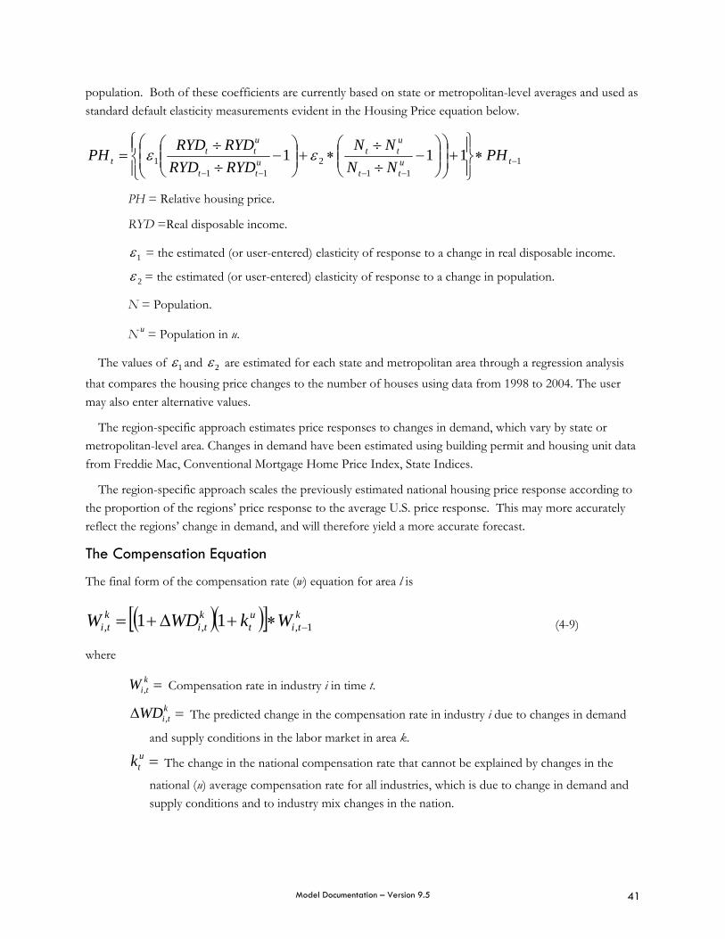
Model Documentation – Version 9.5 41
population. Both of these coefficients are currently based on state or metropolitan-level averages and used as standard default elasticity measurements evident in the Housing Price equation below.
111
211
1 111 −−−−−
∗⎪⎭
⎪⎬⎫
⎪⎩
⎪⎨⎧
+⎟⎟⎠
⎞⎜⎜⎝
⎛⎟⎟⎠
⎞⎜⎜⎝
⎛−
÷÷
∗+⎟⎟⎠
⎞⎜⎜⎝
⎛−
÷÷
= tutt
utt
utt
utt
t PHNNNN
RYDRYDRYDRYDPH εε
PH = Relative housing price.
RYD =Real disposable income.
1ε = the estimated (or user-entered) elasticity of response to a change in real disposable income.
2ε = the estimated (or user-entered) elasticity of response to a change in population.
N = Population.
N u = Population in u.
The values of 1ε and 2ε are estimated for each state and metropolitan area through a regression analysis that compares the housing price changes to the number of houses using data from 1998 to 2004. The user may also enter alternative values.
The region-specific approach estimates price responses to changes in demand, which vary by state or metropolitan-level area. Changes in demand have been estimated using building permit and housing unit data from Freddie Mac, Conventional Mortgage Home Price Index, State Indices.
The region-specific approach scales the previously estimated national housing price response according to the proportion of the regions’ price response to the average U.S. price response. This may more accurately reflect the regions’ change in demand, and will therefore yield a more accurate forecast.
The Compensation Equation
The final form of the compensation rate (w) equation for area l is
( )( )[ ] kti
ut
kti
kti WkWDW 1,,, 11 −∗+Δ+= (4-9)
where
=ktiW , Compensation rate in industry i in time t.
=Δ ktiWD , The predicted change in the compensation rate in industry i due to changes in demand
and supply conditions in the labor market in area k.
=utk The change in the national compensation rate that cannot be explained by changes in the
national (u) average compensation rate for all industries, which is due to change in demand and supply conditions and to industry mix changes in the nation.
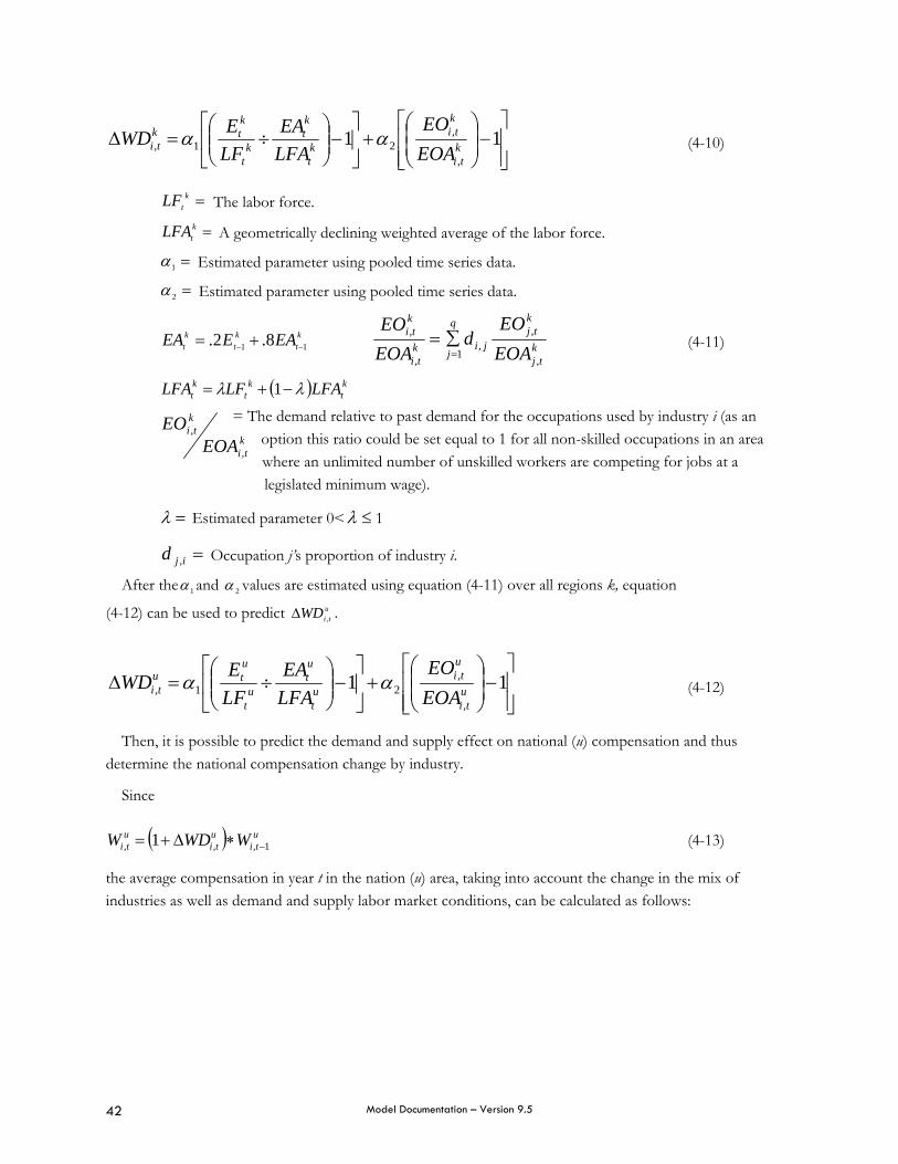
Model Documentation – Version 9.5 42
⎥⎥⎦
⎤
⎢⎢⎣
⎡−⎟
⎟⎠
⎞⎜⎜⎝
⎛+⎥
⎦
⎤⎢⎣
⎡−⎟⎟
⎠
⎞⎜⎜⎝
⎛÷=Δ 11
,
,21, k
ti
kti
kt
kt
kt
ktk
ti EOAEO
LFAEA
LFEWD αα (4-10)
=ktLF The labor force.
=ktLFA A geometrically declining weighted average of the labor force.
=1α Estimated parameter using pooled time series data.
=2α Estimated parameter using pooled time series data.
kt
kt
kt EAEEA 11 8.2. −− += k
tj
ktj
ji
q
jkti
kti
EOAEO
dEOAEO
,
,,
1,
,
=∑= (4-11)
( ) kt
kt
kt LFALFLFA λλ −+= 1
= The demand relative to past demand for the occupations used by industry i (as an option this ratio could be set equal to 1 for all non-skilled occupations in an area where an unlimited number of unskilled workers are competing for jobs at a legislated minimum wage).
=λ Estimated parameter 0< ≤λ 1
=ijd , Occupation j’s proportion of industry i.
After the 1α and 2α values are estimated using equation (4-11) over all regions k, equation
(4-12) can be used to predict utiWD ,Δ .
⎥⎥⎦
⎤
⎢⎢⎣
⎡−⎟
⎟⎠
⎞⎜⎜⎝
⎛+⎥
⎦
⎤⎢⎣
⎡−⎟⎟
⎠
⎞⎜⎜⎝
⎛÷=Δ 11
,
,21, u
ti
uti
ut
ut
ut
utu
ti EOAEO
LFAEA
LFEWD αα (4-12)
Then, it is possible to predict the demand and supply effect on national (u) compensation and thus determine the national compensation change by industry.
Since
( ) uti
uti
uti WWDW 1,,, 1 −∗Δ+= (4-13)
the average compensation in year t in the nation (u) area, taking into account the change in the mix of industries as well as demand and supply labor market conditions, can be calculated as follows:
kti
kti
EOAEO
,
,
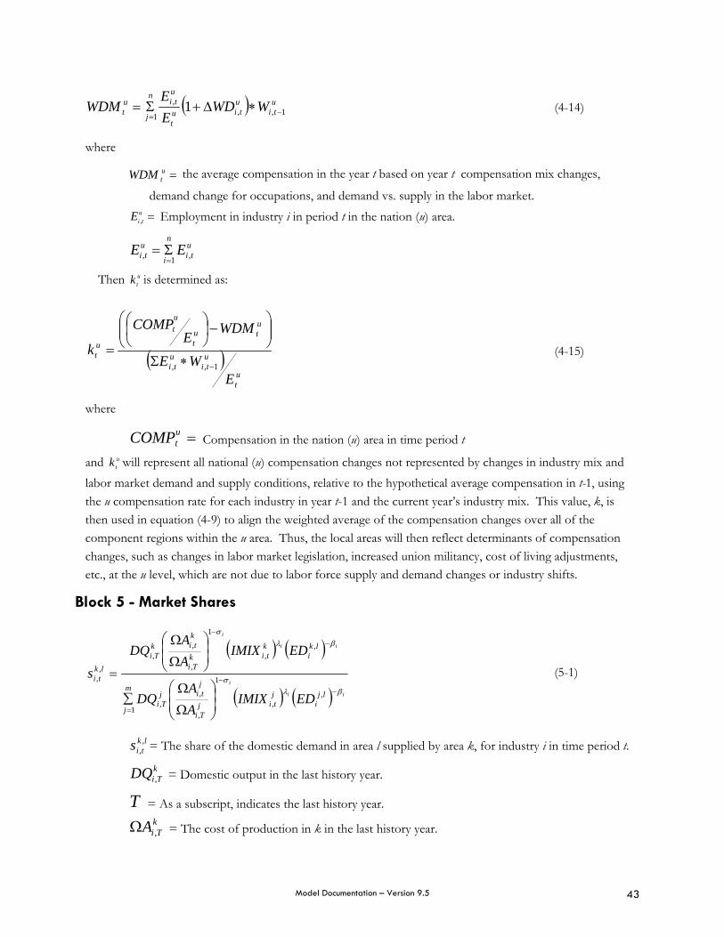
Model Documentation – Version 9.5 43
( ) uti
utiu
t
uti
n
j
ut WWD
EE
WDM 1,,,
11 −=
∗Δ+Σ= (4-14)
where
=utWDM the average compensation in the year t based on year t compensation mix changes,
demand change for occupations, and demand vs. supply in the labor market. =u
tiE , Employment in industry i in period t in the nation (u) area.
uti
n
i
uti EE ,1, =
Σ=
Then utk is determined as:
( )ut
uti
uti
utu
t
tu
ut
EWE
WDMECOMP
k1,, −∗Σ
⎟⎟⎠
⎞⎜⎜⎝
⎛−⎟
⎠⎞
⎜⎝⎛
= (4-15)
where
=tuCOMP Compensation in the nation (u) area in time period t
and utk will represent all national (u) compensation changes not represented by changes in industry mix and
labor market demand and supply conditions, relative to the hypothetical average compensation in t-1, using the u compensation rate for each industry in year t-1 and the current year’s industry mix. This value, k, is then used in equation (4-9) to align the weighted average of the compensation changes over all of the component regions within the u area. Thus, the local areas will then reflect determinants of compensation changes, such as changes in labor market legislation, increased union militancy, cost of living adjustments, etc., at the u level, which are not due to labor force supply and demand changes or industry shifts.
Block 5 - Market Shares
( ) ( )
( ) ( ) ii
i
ii
i
lji
jtij
Ti
jtij
Ti
m
j
lki
ktik
Ti
ktik
Tilk
ti
EDIMIXAA
DQ
EDIMIXAA
DQ
sβλ
σ
βλσ
−−
=
−−
⎟⎟⎠
⎞⎜⎜⎝
⎛
Ω
Ω∑
⎟⎟⎠
⎞⎜⎜⎝
⎛
Ω
Ω
=,
,
1
,
,,
1
,,
1
,
,,
,, (5-1)
lktis ,
, = The share of the domestic demand in area l supplied by area k, for industry i in time period t.
kTiDQ , = Domestic output in the last history year.
T = As a subscript, indicates the last history year. kTiA ,Ω = The cost of production in k in the last history year.
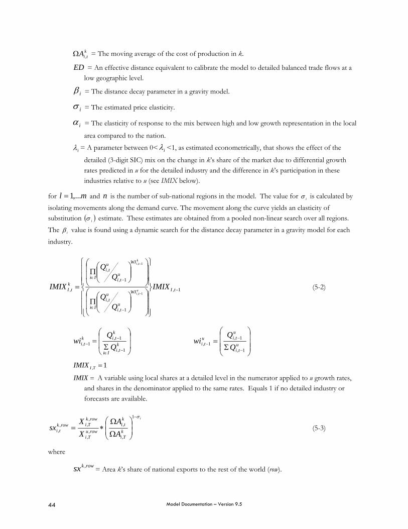
Model Documentation – Version 9.5 44
ktiA ,Ω = The moving average of the cost of production in k.
ED = An effective distance equivalent to calibrate the model to detailed balanced trade flows at a low geographic level.
iβ = The distance decay parameter in a gravity model.
iσ = The estimated price elasticity.
iα = The elasticity of response to the mix between high and low growth representation in the local
area compared to the nation.
iλ = A parameter between 0< iλ <1, as estimated econometrically, that shows the effect of the
detailed (3-digit SIC) mix on the change in k’s share of the market due to differential growth rates predicted in u for the detailed industry and the difference in k’s participation in these industries relative to u (see IMIX below).
for ml ,...1= and n is the number of sub-national regions in the model. The value for iσ is calculated by isolating movements along the demand curve. The movement along the curve yields an elasticity of substitution ( )iσ estimate. These estimates are obtained from a pooled non-linear search over all regions. The iβ value is found using a dynamic search for the distance decay parameter in a gravity model for each industry.
1,
1,
,
1,
,
,1,
1,
−
−∈
−∈
⎪⎪⎪
⎭
⎪⎪⎪
⎬
⎫
⎪⎪⎪
⎩
⎪⎪⎪
⎨
⎧
⎟⎟
⎠
⎞
⎜⎜
⎝
⎛⎟⎟⎠
⎞⎜⎜⎝
⎛Π
⎟⎟
⎠
⎞
⎜⎜
⎝
⎛⎟⎟⎠
⎞⎜⎜⎝
⎛Π
=−
−
tIWI
uti
uti
Ii
WI
uti
uti
Iik
tI IMIX
IMIXu
ti
kti
(5-2)
⎟⎟
⎠
⎞
⎜⎜
⎝
⎛
Σ=
−∈
−− k
tiIi
ktik
ti QQ
wi1,
1,1,
⎟⎟⎟
⎠
⎞
⎜⎜⎜
⎝
⎛
Σ=
−
−− u
ti
utiu
ti QQ
wi1,
1,1,
1, =TIIMIX
=IMIX A variable using local shares at a detailed level in the numerator applied to u growth rates, and shares in the denominator applied to the same rates. Equals 1 if no detailed industry or forecasts are available.
i
kTi
kti
rowuTi
rowkTirowk
ti AA
XX
sxσ−
⎟⎟⎠
⎞⎜⎜⎝
⎛
Ω
Ω∗=
1
,
,,
,
,,,
, (5-3)
where
rowksx , = Area k’s share of national exports to the rest of the world (row).
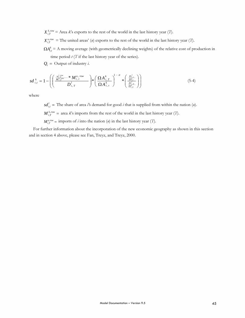
Model Documentation – Version 9.5 45
rowkTiX ,, = Area k’s exports to the rest of the world in the last history year (T).
rowuTiX ,, = The united areas’ (u) exports to the rest of the world in the last history year (T).
ktiA ,Ω = A moving average (with geometrically declining weights) of the relative cost of production in
time period t (T if the last history year of the series). =iQ Output of industry i.
⎟⎟⎠
⎞⎜⎜⎝
⎛⎟⎟⎠
⎞⎜⎜⎝
⎛⎟⎠⎞
⎜⎝⎛
ΩΩ
⎟⎟⎠
⎞⎜⎜⎝
⎛−=
−
Tiu
Til
tiu
til
Tirowu Ti
rowlM
DDDD
tik
Tik
Til
tirowu
Mkti A
AD
Msd
,
,
,,
,,,
,
***
11
,
,
,
,,
,
σ
(5-4)
where
=ltisd , The share of area l’s demand for good i that is supplied from within the nation (u).
=rowkTiM ,, area k’s imports from the rest of the world in the last history year (T).
=rowuTiM ,, imports of i into the nation (u) in the last history year (T).
For further information about the incorporation of the new economic geography as shown in this section and in section 4 above, please see Fan, Treyz, and Treyz, 2000.

Model Documentation – Version 9.5 46
List of References Fan, Wei, Frederick Treyz, and George Treyz. 2000. “An Evolutionary New Economic Geography Model,”
Journal of Regional Science, Vol. 40(4), 671-695.
Fujita, Masahisa, Paul Krugman, and Anthony J. Venables. The Spatial Economy: Cities, Regions, and International Trade. Cambridge, Massachusetts: MIT Press, 1999.
Greenwood, Michael J., Gary L. Hunt, Dan S. Rickman, and George I. Treyz. 1991. “Migration, Regional Equilibrium, and the Estimation of Compensating Differentials,” American Economic Review, Vol. 81(5), 1382-1390.
Rickman, Dan S., Gang Shao, and George Treyz. 1993. “Multiregional Stock Adjustment Equations of Residential and Nonresidential Investment in Structures,” Journal of Regional Science, Vol. 33(2), 207-219.
Treyz, Frederick, and George I. Treyz. 1997. “The REMI Multi-Regional U.S. Policy Analysis Model,” paper presented at the North American Regional Science Association Meetings.
Treyz, George I. 1993. Regional Economic Modeling: A Systematic Approach to Economic Forecasting and Policy Analysis. Norwell, Massachusetts: Kluwer Academic Publishers.
Treyz, George I., Ann F. Friedlaender, and Benjamin H. Stevens. 1977. “Massachusetts Economic Policy Analysis Model.”
Treyz, George I., and Lisa M. Petraglia. 2001. “Consumption Equations for a Multi-Regional Forecasting and Policy Analysis Model,” Regional Science Perspectives in Economic Analysis. Elsevier Science B.V., 287-300.
Treyz, George I., Chris G. Christopher, Jr., and Chengfeng Lou. 1996. “Regional Labor Force Participation Rates,” Regional Economic Models, Inc.
Treyz, George. I., Dan S. Rickman, Gary L. Hunt, and Michael J. Greenwood. 1993. “The Dynamics of U.S. Internal Migration,” The Review of Economics and Statistics, Vol. LXXV, No. 2, May 1993, 209-214.
Weisbrod, Glen, Donald Vary, and George Treyz. 2001. “Project 2-21 – Final Report: Economic Implications of Congestion.” Transportation Research Board, National Cooperative Highway Research Program Report 463. Washington, DC: National Academy Press, 2001.
Model Documentation – Version 9.5 47
Chapter 2: Demographic Component of the REMI Model
Overview The demographic component of the REMI model uses a “cohort-component” method to forecast the population for a region. The components of demographic change are calculated every year for each of the age cohorts by sex and race. The population at the end of the year is equal to the population at the beginning of the year (starting population) plus births and net migration, minus deaths. The rate of change for each of the components depends on both observed historical trends in the region and on forecasted national trends. There are also several types of special populations that have different characteristics than the rest of the population and need to be treated differently. They are military, military dependents, prisoners, and college students.
Historical Data
Population
The model contains historical demographic data starting from the year 1990. Some of this data comes from official sources and some of it is estimated.
The Bureau of Economic Analysis (BEA) provides the total population for each county from its personal income and population summary tables. The BEA uses the population estimates from the U.S. Bureau of the Census. It is important that the population estimates are consistent with the personal income estimates, so the total population data is taken from the BEA instead of directly from the Census in case one bureau revises its estimates and the other does not.
The Census provides population estimates annually in 5-year age groups by sex, race, and Hispanic origin. There are 4 races in the REMI model, White, Black, Other, and Hispanic. The Census treats race and Hispanic origin as two different concepts in accordance with the guidelines from the Office of Management and Budget (OMB). Each person has a race and a separate Hispanic origin attribute, so a Hispanic person may be of any race. From the year 1990 to 1999, the Census asked people whether they were Hispanic or Non-Hispanic and asked them to pick a single race to identify themselves. Starting in 2000, people were asked to select all of the races that apply to them, instead of the race that best describes them. This means that the estimates of population by race are not completely compatible for the years before and after 2000.
Before 2000, the category White in the REMI model includes non-Hispanics who primarily identify themselves as White. Black includes non-Hispanics who primarily identified themselves as Black, and all other non-Hispanics are grouped into Other. Hispanic contains all people who are of Hispanic Origin regardless of their race. Afterwards, the White category includes non-Hispanic people who are White alone, the Black category includes non-Hispanic people who are Black alone, and non-Hispanics of all other races and combinations of races are grouped into Other. Hispanic still contains all people who are of Hispanic Origin, regardless of their race.
As a result of the racial definition changes, the population of some of the races may have made some sudden jumps or drops in the year 2000. The population shifts will show up in the model as economic migration. Although there may be a large jump in the number of economic migrants by race, there will not

Model Documentation – Version 9.5 48
be a large change in the number of economic migrants for the sum of all races, so this population shift will not affect the economic calculations.
Historical population estimates for single years of age are estimated by taking the starting population in the year 1990, applying the components of change by age, and adjusting the ages within each 5-year age group so the total matches the Census estimates.
Components of Change
The Census provides annual estimates of the total number of births, deaths, and net international migrants into each county, which are used to calibrate the county’s birth rates, survival rates, and migration rates.
Birth rates can vary greatly by region and are difficult to calculate for each county because of small sample sizes. State birth rates are calculated by race and age group using data from the Center for Disease Control, National Center for Health Statistics. Regional birth rates are created by adjusting the state rates to fit the total number of births that are estimated by the Census.
The Census publishes its own population projection and the assumptions that are used to generate it, including a natality rate and survival rate forecast. The assumed national survival rates are specific to each age, sex, race, and Hispanic origin. Regional survival rates in the model are estimated by adjusting the national survival rates to fit the total number of deaths estimated in the area.
Net international migration is the net number of people who enter the region from outside the fifty states and District of Columbia. This includes net migration from Puerto Rico and U.S. territories, Armed Forces, permanent migrants, temporary migrants (such as students), refugees, and illegal migrants. Net international migrants in each county are divided up by race according to the data from the state population projections from the Census. Each county in the state has the same racial breakdown of net international migrants as the whole state.
People aged 65 and older who move from one area to another are called retired migrants. They do not respond to economic conditions. Data from the Census 2000 Migration DVD is used to calculate a migration rate by age for each of the counties.
The interregional migrants under the age of 65 are called economic migrants. Economic migrants are calculated as the residual of population growth of the region during the year minus all of the other components of change. The labor force, relative employment opportunity, relative wage rate, and the commodity access index are used, along with the historical economic migration data, to calculate an amenity term for the area which is used in the migration equation to predict future migration.
Population Forecast The changes in birth and survival rates from the Census population projection assumptions file are applied to the last history year regional birth and survival rates to form the forecasted rates. These rates are multiplied by the population by sex, race, and age to predict the number of births and deaths.
The net international migration forecast for the nation by race is also from the Census assumptions files. Each area gets the same percentage of the nation’s net international migrants by race as it had in the last history year. The international migrants acquire the birth rates and survival rates of the area that they move

Model Documentation – Version 9.5 49
into. Births and deaths are calculated for the migrant population by applying the birth and survival rates to half of the migrants, because the migrants arrive during the whole year and will only be in the region for half of the year, on average.
Economic migration is an endogenous calculation in the model. It depends on the economic conditions, the current labor force, and the amenity of the area. Births and deaths are added and subtracted from the economic migrants in the same manner that they are for the international migrants.
Retired migration for the area is calculated using the retired migration rates by age group. If the rate is a positive number, then the net retired migration into the area is based on the size of the 65 and older population in the rest of the nation. Otherwise, the net migration leaving the area is related to the migration rate and size of the over-65 population in the area.
Special Populations Special populations are also estimated by age, sex, race, and Hispanic origin. The special populations are important because they are pockets of the general population that do not appear to age over time and have other special characteristics.
Active Military
The active military consists of people in the full-time duty in the active service of the Army, Navy, Marine Corps, or Air Force. It includes uniformed personnel on the active list, in training, or in military schools. Total active military population data by base is available from the Department of Defense, Statistical Information Analysis Division. National sex and race totals for the active military are from the DoD, Office of Personnel and Readiness publication “Population Representation in the Military Services”. Federal Military employment data from BEA differs from active military strength because federal military includes all active military, Coast Guard, and military reserve members who meet regularly for training. Active military personnel are not part of the labor force, and only active military members have military dependents. The ratio of active military to Federal Military employment is calculated in the last history year, and number of active military personnel in the forecast is calculated by applying that ratio to the forecasted Federal Military employment total.
Active Military Dependents
Active military dependents are the family members that live with active military personnel and move when the person in the military is reassigned to a different base. They are the spouses, children, and other adult family members that depend on an active member of the military. Dependent totals by branch of the military are available from the DoD publication “Selected Manpower Statistics”. The national ratio of active military to dependents is recalculated by branch every year based on new data. This ratio is applied to the active military at each of the bases to estimate the number of dependents.
College Students
College population estimates are very important, because there are more than 15 million people in the United States enrolled in college, and they mostly fall within a very narrow age range. Students that live in places other than their hometowns during the school year are counted by the Census as residents of their new

Model Documentation – Version 9.5 50
towns. It is difficult to estimate college population, because not all of the college students necessarily live in the same county as the college where they are enrolled. Census enrollment data by county, race, and sex are used in combination with data from the Department of Education, National Center for Educational Statistics to estimate the college population of an area by year. College students are assumed to have labor force participation rates lower than the general college-aged population.
Prisoners
Prisoners are estimated using data from the 2000 Census and annual data from the Department of Justice Statistics. The Census data provides a distribution of prisoners by race, sex, and type of facility for each county. The change in prisoners by year is based on state and national level data about local jails and state, federal, and military prisons from the Bureau of Justice Statistics. Prisoners are not included in the labor force.
What Makes Special Populations Special?
For the population estimates to be reasonable, it is important to recognize the special populations because they can comprise a very large portion of the population in an area that does not appear to age over time. In a college town, for example, there may be thousands of people between the ages of 18 and 22 years. Ten years later, there will not be an abundance of 28-to-32-year-olds; instead, the same 18-to-22-year-old bulge in the population will still exist. If special populations were simply not allowed to age, this would create problems in large models that have a large total special population but a small net special population. To model this situation, before the population in an area is aged, all of the special populations are returned to their “home areas”. The special populations estimated in the area are taken out and the estimated special populations from the area that currently exist in other areas are brought back in. The population is then aged one year. New special populations are added to and taken out of the population in the same age distribution as the previous year. In this way, the special population appears not to age and the total population of the nation is allowed to grow normally.
Special populations are also treated differently in the labor force calculations. Labor force participation rates are only applied to the civilian, non-institutional population.
Labor Force Historical labor force totals by county are taken from the Bureau of Labor Statistics. Participation rates by race and age are calculated using the relative compensation rate, employment opportunity, demographic characteristics, and national participation rates. They are calibrated in the history so the labor force will be consistent with the data reported by the BLS. The participation rates are multiplied by the civilian non-institutional population to generate the labor force. Forecasted national rates from BLS are used in the participation rate equation to help shape the participation rates in the model forecast.
Model Documentation – Version 9.5 51
Chapter 3: Data Sources and Estimation Procedures
A. Primary Historical Data
BEA
The primary national, state, and county data source for REMI Policy Insight is the Bureau of Economic Analysis (BEA) employment, compensation, and personal income series (which includes total population). The BEA data is available for the nation and states at the summary level (94 industries), and for counties at the sector level (24 industries).
Employment
The BEA employment series for states and local areas comprises estimates of the number of jobs, full-time plus part-time, by place of work. Full-time and part-time jobs are counted at equal weight. Employees, sole proprietors, and active partners are included, but unpaid family workers and volunteers are not included.
Employment can be measured either as a count of workers or as a count of jobs. In the former case, an employed worker is counted only once; in the latter case, all jobs held by the worker are counted. The state and county employment estimates are a count of the number of jobs, so that, as with the earnings estimates, a worker’s activity in each industry and location of employment is reflected in the measure.
Proprietors’ employment consists of the number of sole proprietorships and the number of partners in partnerships. The description “by place of work” applies to the wage and salary portion of the series, and, with relatively little error, to the entire series. The proprietors’ employment portion of the series, however, is more nearly by place of residence because, for non-farm sole proprietorships, the estimates are based on IRS tax data that reflect the address from which the proprietor’s individual tax return is filed, which is usually the proprietor’s residence. The non-farm partnership portion of the proprietors’ employment series reflects the tax-filing address of the partnership, which may be either the residence of one of the partners or the business address of the partnership.
The employment estimates are designed to be consistent with the estimates of wage and salary disbursements and proprietors’ income that are part of the personal income series. The employment estimates are based on the same sets of source data as the corresponding earnings estimates, and are prepared with parallel methodologies. Two forms of proprietors’ income - the income of limited partnerships and the income of tax-exempt cooperatives - have no corresponding employment estimates.
Employment in industries covered by the UI programs
The estimates of about 95 percent of wage and salary employment are derived from tabulations by the state employment security agencies (ESAs) from their state employment security reports (form ES-202). These tabulations summarize the data from the quarterly UI contribution reports filed with a state ESA by the employers subject to that state’s UI laws. Employers usually submit reports for each operating establishment, classified by county and industry. However, in some cases, an employer may group very small establishments in a single “statewide” report without county designation. Each quarter, the various state ESAs submit the ES-202 tabulations to the Bureau of Labor Statistics (BLS), which provides the data to BEA. The tabulations present monthly employment and quarterly wages for each county in North American Industry Classification System (NAICS) four-digit and five-digit industry detail.

Model Documentation – Version 9.5 52
BEA adds several million administrative records received from the states and the District of Columbia to its database annually. The records are checked for major errors by several computerized edit routines. One edit routine analyzes the current quarter county data for invalid NAICS codes, duplicate records, and records that contain no data. Another edit routine calculates expected county-level average employment and average wage estimates on a quarterly basis at the NAICS industry group level, based on percentage changes for that quarter in the previous two years. If the difference between the actual numbers and the estimated numbers exceeds established limits, the record is identified for further review. Anomalies that remain unreconciled after reviewing comments and other supporting data are referred back to BLS for further investigation.
The basic procedure for preparing the local area estimates of wage and salary employment for each UI-covered industry is to average the 12 monthly ES-202 employment observations and to allocate the higher-level geographic totals (counties add up to states, and states add up to the nation) in proportion to the averaged series. However, ES-202 employment does not precisely meet the statistical and conceptual requirements for BEA’s employment estimates. Consequently, the data must be adjusted to meet the requirements more closely. The necessary adjustments affect both the industrial and geographic patterns of county employment.
Employment not covered by the UI programs
• Railroads ― The railroad industry is covered by its own unemployment insurance program, which is administered by the Railroad Retirement Board (RRB), rather than by the state UI system. Data suitable for estimating local area employment of railroads are available from the RRB only on a place-of-residence basis. Because BEA’s employment estimates are designed to conform conceptually and statistically to the place-of-work earnings estimates, the RRB data are adjusted to a place-of-work basis by using journey-to-work data from the 1990 Census of Population. The national totals for all railroad companies combined are allocated to counties in proportion to the adjusted RRB series.
• Private households ― For this largely non-covered industry - mainly domestic servants - the national employment estimates are allocated to counties in proportion to place-of-work private household employment from the 1990 Census journey-to-work data.
• Farm labor contractors ― This industry is classified in agricultural services rather than in farms. The UI coverage in Arizona and California is complete enough to permit the use of the ES-202 data for both the state and county estimates, but most state UI programs only partially cover this industry. For these states, the county estimates of farm labor contractor employment are based on the geographic distribution of expenditures for contract labor reported in the Census of Agriculture.
• Private elementary and secondary schools ― Private elementary and secondary schools are treated as a non-covered industry because religiously affiliated elementary and secondary schools, which account for most of the employment in this industry, remain largely outside the scope of the UI program. The state estimates of private elementary and secondary school employment are primarily based on the employment reported annually by the Census Bureau’s County Business Patterns (CBP). The CBP data are tabulated from the administrative records of the social security program ― old-age, survivors, disability, and hospital insurance ― and are more complete for elementary and secondary schools than the data prepared under the UI program. The social security program, although exempting nonprofit religious organizations ― including schools ― from mandatory coverage, has elective

Model Documentation – Version 9.5 53
coverage provisions that have resulted in broad participation among religiously affiliated elementary and secondary schools. In about half of the states, the UI coverage of elementary and secondary schools is complete enough to permit the use of ES-202 data as the basis for the county employment estimates. For the other states, the county estimates are based on the best available series of private elementary and secondary school employment chosen from data published by state departments of education, data from the U.S. Department of Education’s 1998 survey of private elementary and secondary schools, or data from CBP, which cannot be used more generally because they are frequently suppressed at the county level to prevent disclosures.
• Religious membership organizations ― The Federal Unemployment Tax Act permits the states to exclude religious membership organizations from mandatory UI coverage. Although most state UI laws do have some provisions for elective coverage, less than 10 percent of the national total employment of religious membership organizations is covered by UI. Therefore, the county estimates of the employment of religious membership organizations are based on CBP data. The CBP data are adjusted by allocation to sum to the BEA national employment totals for this industry.
• Military ― County military employment is measured as the number of military personnel assigned to active duty units that are stationed in the area plus the number of military reserve unit members. The estimates of active duty employment for the Army, Air Force, Navy, Marine Corps, and Coast Guard are based on the annual averages of 12 monthly observations, for a given year, from reports received from each branch of service. Navy personnel assigned to ships and other mobile units and Marines assigned to Fleet Marine Force units are measured according to the units’ home ports rather than their actual locations as of the reporting date. The measure of the employment of the military Reserves ― including the National Guard ― is confined to members of reserve units that meet regularly for training. The state estimates are based on fiscal year-ending September 30 tabulations of military reserve pay provided by the Army, Air Force, Navy, Marine Corps, and Coast Guard. For consistency with the BEA estimates of military reserve wages, the state totals of military reserve employment are allocated to counties in proportion to civilian population.
• “Other” ― In the local area employment series, this category consists of the number of U.S. residents employed in the United States by international organizations and by foreign embassies and consulates. The category differs from “rest-of-the-world” -- the corresponding category in the national employment estimates ― in that “rest-of-the-world” also includes the net flow of international border workers ― i.e., U.S. residents working across the border in Canada and foreign residents working in the United States. The border workers are not reflected in the county employment estimates. The county estimates of “other” employment are made by allocating the national totals for all years to counties in proportion to estimated 1968 administrative expenses of international and foreign organizations operating in the United States. The administrative expenses series was prepared by the BEA.

Model Documentation – Version 9.5 54
Wage and salary disbursements
Wage and salary disbursements consist of the monetary remuneration of employees, including corporate officers’ salaries and bonuses, commissions, pay-in-kind, incentive payments, and tips. It reflects the amount of payments disbursed, but not necessarily earned during the year.
Wage and salary disbursements are measured before deductions, such as social security contributions and union dues.
In recent years, stock options have become a point of discussion. Wage and salary disbursements include stock options of nonqualified plans at the time that they have been exercised by the individual. Stock options are reported in wage and salary disbursements. The value that is included in wages is the difference between the exercise price and the price that the stock options were granted.
All state and local area dollar estimates are in current dollars (not adjusted for inflation).
Wages and salaries for the military services
The estimates of wages and salaries for the military services consist of the estimates of cash wages (including allowances) of full-time personnel of the armed services (including the Coast Guard), the estimates of cash wages of the members of the Reserves including the National Guard, and the estimates of pay-in-kind received by the full-time and reserve enlisted personnel of the armed services.
Compensation
Compensation of employees, received, is the sum of Wage and Salary Disbursements and Supplements to Wages and Salaries.
Personal income and components
Personal Income is the income that is received by all persons from all sources. It is calculated as the sum of wage and salary disbursements, supplements to wages and salaries, proprietors’ income with inventory valuation and capital consumption adjustments, rental income of persons with capital consumption adjustment, personal dividend income, personal interest income, and personal current transfer receipts, less contributions for government social insurance.
The personal income of an area is the income that is received by, or on behalf of, all the individuals who live in the area; therefore, the estimates of personal income are presented by the place of residence of the income recipients.
Supplements to wages and salaries
This component of personal income consists of employer contributions for employee pension and insurance funds and of employer contributions for government social insurance.

Model Documentation – Version 9.5 55
Employer contributions for employee pension and insurance funds
This component of personal income consists of employer payments to private and government employee retirement plans, private group health and life insurance plans, privately administered workers’ compensation plans, and supplemental unemployment benefit plans.
Employer contributions for government social insurance
These contributions, which are subtracted in the calculation of personal income as part of contributions for government social insurance, consist of employer payments under the following Federal and state and local government programs: Old-age, survivors, and disability insurance (OASDI); hospital insurance (HI); unemployment insurance; railroad retirement; government employee retirement; pension benefit guarantee; veterans’ life insurance; publicly-administered workers’ compensation; military employee programs (veterans’ life and military medical insurance); and temporary disability insurance. The contributions are excluded from personal income by definition, but, as part of supplements to wages and salaries, are included in earnings by place of work.
Proprietors’ income
This component of personal income is the current-production income (including income in kind) of sole proprietorships and partnerships and of tax-exempt cooperatives. Corporate directors’ fees are included in proprietors’ income, but the imputed net rental income of owner-occupants of all dwellings is included in rental income of persons. Proprietors’ income excludes dividends and monetary interest received by non-financial business and rental incomes received by persons not primarily engaged in the real estate business; these incomes are included in dividends, net interest, and rental income of persons, respectively.
Rental income of persons with capital consumption adjustment
Rental income is the net income of persons consisting of income from the rental of real property except for the income of persons primarily engaged in the real estate business; the imputed net rental income of the owner-occupants of non-farm dwellings; and the royalties received from patents, copyrights, and rights to natural resources.
The Capital Consumption Adjustment is the difference between private consumption of fixed capital (CFC) and private capital consumption allowances. Private CFC is a charge for the using up of private fixed capital. It is based on studies of prices of used equipment and structures in resale markets. Private capital consumption allowances consist of tax-return-based depreciation charges for corporations and non-farm proprietorships and of historical-cost depreciation, calculated by BEA, for farm proprietorships, rental income of persons, and nonprofit institutions.
Personal dividend income
This component of personal income is the dividend income of persons. It consists of the payments in cash or other assets, excluding the corporation’s own stock, made by corporations located in the United States or abroad to persons who are U.S. residents. It excludes that portion of dividends paid by regulated investment companies (mutual funds) related to capital gains distributions.

Model Documentation – Version 9.5 56
Personal interest income
This component of personal income is the interest income (monetary and imputed) of persons from all sources.
Personal current transfer receipts
This component of personal income is payments to persons for which no current services are performed. It consists of payments to individuals and to nonprofit institutions by Federal, state, and local governments and by businesses.
Government payments to individuals include retirement and disability insurance benefits, medical payments (mainly Medicare and Medicaid), income maintenance benefits, unemployment insurance benefits, veterans’ benefits, and Federal grants and loans to students. Government payments to nonprofit institutions exclude payments by the Federal Government for work under research and development contracts. Business payments to persons consists primarily of liability payments for personal injury and of corporate gifts to nonprofit institutions.
Contributions for government social insurance
These contributions, which are subtracted in the calculation of personal income, consist of employee and self-employed contributions for government social insurance and employer contributions for government social insurance.
Employee and self-employed contributions for government social insurance
These contributions, which are subtracted in the calculation of personal income, consist of the contributions, or payments, by employees, by the self-employed, and by other individuals who participate in the following government programs: old-age, survivors’, and disability insurance (Social Security); hospital insurance; supplementary medical insurance; unemployment insurance; railroad retirement; veterans’ life insurance; and temporary disability insurance. These contributions are excluded from personal income by definition, but the components of personal income upon which these contributions are based – mainly wage and salary disbursements and proprietors’ income – are presented gross of the contributions.
Adjustment for residence
The adjustment for residence is the net inflow of the net labor earnings of interarea commuters.
The state and county estimates of personal income are presented by the state and county of residence of the income recipients. However, the source data for most of the components of wage and salary disbursements, other labor income, and personal contributions for social insurance by employees are on a place-of-work basis. Consequently, a residence adjustment is made to convert the estimates based on these source data to a place-of-residence basis.
The method of calculating place-of-work income requires two main sources. The first source is the net Residence Adjustment (RA), which is provided by the Bureau of Economic Analysis (BEA). A Resident Adjustment value for County X is simply the total outflow of workers’ dollars minus the total inflow of workers’ dollars for that county, where outflow dollars are wages earned in County X by residents of another county and inflow dollars are wages earned in another county by residents of County X. The second source
Model Documentation – Version 9.5 57
is Journey to Work (JTW) data, which is calculated from the U.S. Census. This data is a comprehensive matrix of the number of employees and their average wages from each county to every other county.
While the Residence Adjustment calculation provides net dollar flows for each county, it does not tell us how much of a county’s RA goes to and comes from specific counties. The JTW data provides these ratios and allows us to build models with accurate regional dollar flows. The decennial dollar flows in the JTW matrix are normalized to annual Residence Adjustment values to keep the flows current and accurate. With this county-level data, we can then calculate intra-regional dollar flows.
Population
BEA uses the Census Bureau’s midyear population estimates. Except for college students and other seasonal populations, which are measured on April 1, the population for all years is estimated on July 1.
Disclosure avoidance procedures
Like other statistical agencies, the Bureau of Economic Analysis (BEA) is legally required to safeguard the confidentiality of the information that it receives. In addition, like other agencies, it must balance its responsibility to avoid disclosing confidential information with its responsibility to release and to publish as much information as possible. It balances these responsibilities by presenting the estimates for regions, states, and local areas only at the North American Industry Classification System (NAICS) subsector level, even though it receives source data at the NAICS four- and five-digit industry levels.
Most of the data series that BEA receives from other agencies are not confidential. The agencies summarize this data to aggregate totals by program and by state or county, so that each record, or data cell, contains data for enough individuals or establishments to preclude the identification of the data for a specific individual or establishment and, therefore, to preclude the disclosure of confidential information.
However, the ES-202 tabulations that BEA receives from the Bureau of Labor Statistics (BLS) include records that would disclose confidential information. The confidential information on wages and salaries for some business firms is identifiable from the state and county estimates of wages and salaries at the NAICS subsector level that are derived from the ES-202 data.
To prevent either the direct or the indirect disclosure of the confidential information, BEA uses the BLS state and county nondisclosure file.
BEA uses as many BLS nondisclosure cells as possible, but cannot use some of them for various reasons. The most important reasons are that the industry structure published by BEA does not exactly match NAICS subsector detail provided by BLS and that BEA does not use ES-202 data for the farm sector. When BEA drops BLS nondisclosure cells, other cells must be selected to prevent the disclosure of confidential information. In order to determine which estimates should be suppressed, the total wages and salaries file and the wages-and-salaries-nondisclosure file are used to prepare a multidimensional matrix. This matrix is tested, and the estimates that should be suppressed are selected.
BLS
The second major source of historical data used by REMI is from the Bureau of Labor Statistics (BLS). These data pertain to workers covered by State unemployment insurance (UI) laws and Federal civilian

Model Documentation – Version 9.5 58
workers covered by the Unemployment Compensation for Federal Employees (UCFE) program. The data for both private sector and public sector workers are reported to the BLS by the employment security agencies of the 50 States, the District of Columbia, Puerto Rico, and the Virgin Islands as part of the Quarterly Census of Employment and Wages (QCEW) program. The QCEW, also called ES-202, was formerly known as the Covered Employment and Wages (CEW). REMI uses their annual average employment and total annual wages at the summary level for all counties and states.
Employment
In general, QCEW monthly employment data represent the number of covered workers who worked during, or received pay for, the pay period that included the 12th day of the month. Virtually all workers are reported in the State in which their jobs are physically located.
Covered private industry employment includes most corporate officials, executives, supervisory personnel, professionals, clerical workers, wage earners, piece workers, and part-time workers. It excludes proprietors, the unincorporated self-employed, unpaid family members, and certain farm and domestic workers.
Persons on paid sick leave, paid holiday, paid vacation, and the like are included. Persons on the payroll of more than one firm during the period are counted by each UI-subject employer if they meet the employment definition noted above. Workers are counted even though, in the latter months of the year, their wages may not be subject to unemployment insurance tax. The employment count excludes workers who earned no wages during the entire applicable pay period because of work stoppages, temporary layoffs, illness, or unpaid vacations.
Employment data reported for Federal civilian employees are a byproduct of the operations of State Employment Security Agencies in administering the provisions of Title XV of the Social Security Act—the program of Unemployment Compensation for Federal Employees. Federal employment data are based on reports of monthly employment and quarterly wages submitted each quarter to State agencies for all Federal installations with employees covered by the act, except for certain national security agencies, which are omitted for security reasons.
Employment of all Federal agencies for any given month is based on the number of persons who worked during or received pay for the pay period that included the 12th of the month.
Wages
Total wages. Covered employers in most states report total compensation paid during the calendar quarter, regardless of when the services were performed. A few state laws, however, specify that wages be reported for or be based on the period during which services are performed rather than the period during which compensation is paid. Under most state laws or regulations, wages include bonuses, stock options, severance pay, the cash value of meals and lodging, tips and other gratuities, and, in some states, employer contributions to certain deferred compensation plans such as 401(k) plans.
Covered employer contributions for old-age, survivors, and disability insurance (OASDI), health insurance, unemployment insurance, workers’ compensation, and private pension and welfare funds are not reported as wages. Employee contributions for the same purposes, however, as well as money withheld for income taxes, union dues, and so forth, are reported even though they are deducted from the worker’s gross pay.

Model Documentation – Version 9.5 59
Average wages. Average annual wages per employee for any given industry are computed by dividing total annual wages by annual average employment. A further division by 52 yields average weekly wages per employee. Annual pay data only approximate annual earnings because an individual may not be employed by the same employer all year or may work for more than one employer at a time.
Average weekly or annual pay is affected by the ratio of full-time to part-time workers, as well as by the numbers of individuals in high-paying and low-paying occupations. When comparing average pay levels between States and industries, data users should take these factors into consideration. For example, industries characterized by high proportions of part-time workers will show average wage levels appreciably less than the weekly pay levels of regular full-time employees in these industries. The opposite is true of industries with low proportions of part-time workers, or industries that typically schedule heavy weekend and overtime work. Average wage data also may be influenced by work stoppages, labor turnover, retroactive payments, seasonal factors, and bonus payments.
Disclosure restrictions
In accordance with BLS policy, data reported under a promise of confidentiality are not published and are used only for specified statistical purposes. BLS withholds publication of UI-covered employment and wage data for any industry level when necessary to protect the identity of cooperating employers. Totals at the industry level for the States and the Nation include the non-disclosable data suppressed within the detailed tables. However, these totals cannot be used to reveal the suppressed data.
Imputed data
To reduce the effect of the exclusion of data that occurs because of late reporting by covered private and government employers, State agencies impute employment and wages for such employers and include them in each quarterly report. Corrections to data that may be entered after a report is filed will include replacement of imputations with reported data to the extent possible. Imputations are calculated at the individual establishment level, normally using historical data reported by the employer. Sometimes, trends reported by employers in the same industry or information obtained from other sources is also used. If a report remains delinquent for more than one quarter and research shows that it is still active, the data for the establishment will again be imputed.
CBP
The final source of employment and wage data is County Business Patterns (CBP). County Business Patterns is an annual series that provides subnational economic data by industry and covers most of the country’s economic activity. The series excludes data on self-employed individuals, employees of private households, railroad employees, agricultural production employees, and most government employees. This data is available at a very detailed level, and while it has many suppressions due to confidentiality requirements, its advantage is that when the data is suppressed, ranges for the establishments are supplied. This provides some basis from which to make a rough estimate of employees in that industry in the absence of any other information.

Model Documentation – Version 9.5 60
Establishments
An establishment is a single physical location at which business is conducted or services or industrial operations are performed. It is not necessarily identical with a company or enterprise (firm), which may consist of one or more establishments. When two or more activities are carried on at a single location under a single ownership, all activities generally are grouped together as a single establishment. The entire establishment is classified on the basis of its major activity and all data are included in that classification.
Establishment-size designations are determined by paid employment in the mid-March pay period. The size group “1 to 4” includes establishments that did not report any paid employees in the mid-March pay period but paid wages to at least one employee at some time during the year.
Establishment counts represent the number of locations with paid employees any time during the year. This series excludes governmental establishments except for wholesale liquor establishments (NAICS 4228), retail liquor stores (NAICS 44531), Federally-chartered savings institutions (NAICS 522120), Federally-chartered credit unions (NAICS 522130), and hospitals (NAICS 622).
Payroll
Total payroll includes all forms of compensation, such as salaries, wages, reported tips, commissions, bonuses, vacation allowances, sick-leave pay, employee contributions to qualified pension plans, and the value of taxable fringe benefits. For corporations, it includes amounts paid to officers and executives; for unincorporated businesses, it does not include profit or other compensation of proprietors or partners. Payroll is reported before deductions for Social Security, income tax, insurance, union dues, etc. First-quarter payroll consists of payroll during the January-to-March quarter.
Mid-March Employment
Paid employment consists of full- and part-time employees, including salaried officers and executives of corporations, who are on the payroll in the pay period including March 12. Included are employees on paid sick leave, holidays, and vacations; not included are proprietors and partners of unincorporated businesses.
Data Withheld from Publication
In accordance with U.S. Code, Title 13, Section 9, no data are published that would disclose the operations of an individual employer. The number of establishments in an industry classification and the distribution of these establishments by employment-size class are not considered to be disclosures, so this information may be released even though other information is withheld from publication.
Estimation of Data Suppressions in Major Regions and States
The current solving methodology is to use an optimization routine to minimize a constrained quadratic loss function. In order to begin this process, we obtain initial estimates and variances from regressions which will be used in our loss function. Once there are estimates, variances, and constraints for all suppressed points within the data set, we process that year. For each year, systems of suppressions can be formed that are all linearly dependent. These systems are defined by a sector-level industry that has suppressions and a Major Region containing the states. We pass each system of suppressions through an optimization procedure that finds the solution set of estimates that minimizes the total variance of the system while still obeying all of the
Model Documentation – Version 9.5 61
regional and industrial constraints. If all the final estimates are positive (with the exception of personal income data, which may have legitimate negative values), the solution set is accepted.
Estimation of Data Suppressions in Counties
There are too many suppressions in the county data to allow the optimization function to solve, so instead we are using a series of RAS methods (bi-proportional adjustment of matrices). First we estimate all of the sector-level industry employment data, making sure that the sum of the industries equals total employment for the county, and the sum of each industry across all counties in a state equals that industry’s employment in that state.
We use the midpoint of the maximum and minimum values calculated from the constraints (similar to calculation for states) as starting values to use in the suppressed cells for the RAS. Next, we repeat this process for the earnings by industry data, as well as the compensation by industry data. This leaves us with sector-level data for employment and summary-level data for earnings and compensation, but no wage data by industry, and we need to disaggregate employment to the summary level.
The first data to be disaggregated to the summary level (REMI’s 70 industries) is compensation. While some of this data is available from the BEA, there are still a large number of suppressions at this level. We bring in the BLS QCEW wage data at the county level. This data also has suppressions, so the first step is to estimate the missing values. This is initially done for all states and industries (making sure they add up to the nation). We use the CBP state wage data in order to start off with reasonable values for the RAS (where this data is suppressed, we estimate the value by multiplying the number of establishments in each size class by the midpoint of the employment size for that class, and then sum them together for each industry). Once the BLS wage state data is filled in to be internally consistent, we then use it as totals for estimating the suppressed BLS wage county data. For this step we start each missing county value with 1. Once complete, we change each BLS zero value to one (since BEA includes proprietors in their definition and BLS does not, it is possible to have zero values in the BLS data and non-zero values in the BEA data) and then run a final set of RAS procedures against the county BEA summary data and the county BEA sector data. This gives us complete summary-level industry data for every county in the US that is internally consistent with BEA’s reported state and county data.
In order to disaggregate the employment to the summary level, we use our recently estimated BEA compensation data at the state and county level. The BEA compensation data is scaled by the state compensation-to-employment ratio before it is used as a starting value for estimating employment. We change any negative values in our starting estimates to a very small value (0.1) in order to prevent negative numbers from entering into the RAS, since employment cannot be negative (although under normal circumstances there should be no negative starting values). We then run a final set of RAS procedures against the state BEA summary data and the county BEA sector data. This gives us complete summary-level industry employment data for every county in the US that is internally consistent with BEA’s reported state and county data.
The wages and personal income are done with a process that is similar to the employment process, but involves some additional checks and balances. As it was with compensation, some of the summary-level BEA county data does exist. For those values that are suppressed, we use our recently estimated BEA

Model Documentation – Version 9.5 62
compensation data, scaled by the state compensation to wages/personal income ratio (as appropriate), as starting values. If any of the wage starting values are less than or equal to zero, we raise them to a small positive value (0.1) as they cannot be negative. If any of the personal income starting values are equal to zero, we raise them to a small positive value (0.1) because BEA suppressed values cannot be zero. We then run a final set of RAS procedures against the county BEA summary data and the county BEA sector data. This gives us complete summary-level industry employment data for every county in the US that is internally consistent with BEA’s reported state and county data.
While our methodology yields the complete, detailed, and internally consistent data sets required by the model, one must keep in mind that there is always more than one possible solution, so, while we have generated “a” solution, it is not necessarily “the” solution. The government goes to great length to suppress data in such a way that the real values cannot be determined. Our solution is not perfect, but we believe for the most part that it is reasonable.
B. Supplementary Historical Data Fuel Cost Data
State-specific relative fuel costs for three types of fuel (electricity, natural gas, residual fuel) are calculated for the industrial (all manufacturing) and commercial (all non-manufacturing) sectors of the model based on unit cost data obtained from the Energy Information Administration, State Price and Expenditure Report.
Fuel Weight Data
Total energy expenditure estimates by sector (residential, commercial, industrial, transportation, and electric utilities), by type (total, electricity, natural gas), and by state are obtained for a recent year from the Energy Information Administration. Residual energy is calculated as total minus electricity and natural gas. Fuel weights are then calculated for each state by sector (the proportion of total fuel expenditures that are electricity, natural gas, and residual); the weights should add up to 1. The industrial sector fuel weights are applied to the manufacturing industries, transportation to transportation industries, electric utilities to utilities industries, and commercial to everything else. The residential sector is not used.
Tax Data
To calculate the cost of capital variable, the model requires both state-specific and national-average corporate profit and property tax rates. In the absence of a consistent and complete data source, the tax rates are estimated as follows.
State and US corporate profit tax rates are defined as the amount of tax collections divided by the amount of corporate profits. The tax collections are found in the Government Finances (Revenue) publication and are converted from fiscal year to calendar year. Profits for states are constructed by sharing the national corporate profits to each state based on gross state product. The effective tax rate is simply the tax collections divided by the estimated profits. Corporate profits for the US are taken from the Survey of Current Business.
State and US property tax rates are defined as the amount of tax collections divided by the level of residential and nonresidential capital stock. Again, tax collections are taken from the Government Finances (Revenue) publication, and converted from fiscal to calendar year. Nonresidential capital stock is calculated
Model Documentation – Version 9.5 63
by estimating the state’s share of national nonresidential capital stock based on estimated profits (see above). Residential capital is estimated similarly, but disposable income is used as the weight. U.S. investment and capital stock data for residential and nonresidential structures are also found in the Survey of Current Business.
Cost of Capital Data
In addition to the tax rates described above, exogenous variables for the cost of capital equation include Moody’s AAA bond rates, investment tax credit rates, and the proportion of business capital financed by bonds and loans. The latter is estimated from the Quarterly Financial Report for Manufacturing, while all of the other variables are taken from the Survey of Current Business.
Housing Price Data
State-specific median values of owner-occupied housing units are obtained from the Census of Housing for the year 2000. The National Association of Realtors’ regional and metropolitan growth rates for median sales price of existing single-family homes are then used to estimate state housing prices after 2000. To determine the national housing price figure, from which selling price for real estate relative to the U.S. is calculated, the Census of Housing value is used for 2000, and the growth rate from the National Association of Realtors’ national data is applied after 2000. County-specific median values of owner-occupied housing units are also obtained from the Census of Housing for 2000. State and metropolitan housing price values are used to extend the series beyond 2000.
C. National Forecast Data BLS Forecast Data
The REMI model’s baseline national forecast is primarily based on the BLS Employment Outlook: 2004-2014, published in the November 2005 issue of the Monthly Labor Review. Input-output, final demand, and value added data are developed by the U.S. Bureau of Labor Statistics in the Office of Occupational Statistics and Employment Projections.
For the 2014 projections, input-output, final demand, and value added data were developed for the years 2001-2004 and projected year 2014. Historical tables are provided in both nominal (current) dollars and in 2000 chain-weighted real dollars. The projected tables are provided in real dollars only.
Dollar value matrices are expressed in millions of dollars rounded to three decimal places. Therefore, they may not add exactly to their totals due to rounding error.
These data are based on the 2002 North American Industrial Classification System (NAICS) and the U.S. Department of Commerce’s Bureau of Economic Analysis (BEA) unpublished revised 1997 benchmark input-output tables.
Input-output data shows the flow of commodities from production through intermediate use by industries and purchases by final users. This data is developed as a set of matrices or tables for each year.
The “USE” matrix contains the sales of commodities sold to intermediate consumers and final demand. In addition, it contains the intermediate inputs and value added factors of production to industries for the production of their product. Each column sums to its respective industry output. Each row sums to its respective commodity output.

Model Documentation – Version 9.5 64
The “MAKE” matrix details the production of commodities by industries. Each row sums to industry output and each column sums to commodity output.
The “FD” matrix is a detailed set of 204 final demand types. Each of the 204 columns is distributed across the 200 commodities identified in the input-output system. This matrix is the final demand “bridge” table, showing detailed purchases for 204 categories of expenditures for the year specified in the matrix name.
For the years 2001-2004 and 2014, REMI converts the industry-by-commodity USE matrix and the commodity-by-industry MAKE matrix into an industry-by-industry input-output table of flows, and subsequently a matrix of coefficients. The FD matrix is converted into a bridge matrix of coefficients.
For the non-benchmark years between 2004 and 2014, a linear interpolation method is used to estimate the coefficients. The 2014 coefficients are held fixed forward to 2050.
The BLS includes as “special industries” noncomparable imports, scrap, and used and secondhand goods. For noncomparable imports and used and secondhand goods, there is no production in the United States, and thus no domestic commodity or industry output.
For scrap, there is domestic production, although that production is not by a “scrap” industry, but by other industries as a part of the production of their output. For REMI purposes, we need to account for these values in our industry-by-industry matrix. For scrap and used and secondhand goods, the great majority of which are automobiles, we made the assumption that most of these goods would at some point pass through the wholesale industry, so we simply aggregated them with wholesale. For noncomparable imports, we added the values (which are negative) to the industry that “used” these imported goods (the commodity by industry diagonal in the USE table), and then balanced the table by subtracting them from the commodity by imports column in the demand table.
The Office of Occupational Statistics and Employment Projections (OOSEP) develops output, price, and employment data for use in the Bureau’s biennial economic and employment projections. The most recent set of projections were developed for the year 2014 with data for 200 detailed industries and 84 aggregate sectors. The projections were published in the November 2005 issue of the Monthly Labor Review.
The output measures follow the definitions and conventions used by the Bureau of Economic Analysis (BEA) in its input-output tables, published every five years. These industry output measures are based on producer’s value and include both primary and secondary products and services. The main data sources for compiling the output time series for manufacturing industries are the Census Bureau’s Annual Survey of Manufactures. Data sources for nonmanufacturing industries are more varied. They include the Census Bureau’s Service Annual Survey, the BEA’s National Income and Product Accounts (NIPA) data on new construction and personal consumption expenditures, IRS data on business receipts, and many other sources. The constant dollar industry output estimates for the most recent years are based on BLS employment data and trend projections of productivity. The output series are benchmarked to the industry/commodity outputs from the unpublished revised BEA 1997 NAICS-based input-output tables, which were adjusted by BLS to reflect the 2002 NAICS revision, NIPA revisions, and to place the tables more consistently on a NAICS basis.

Model Documentation – Version 9.5 65
The annual price data are developed in a manner so as to conform to BEA’s National Income and Product Accounts. For manufacturing, they are based on industry sector price index data collected by BLS, and are chain-weighted from the four-digit NAICS to OOSEP’s detailed industry sectors. Nonmanufacturing prices, developed at the level of OOSEP’s detailed industry sectors, use a variety of different sources, in many instances the BLS consumer price index data. In industries where such underlying price data have not yet been developed, imputations of price change are made from other data series. All aggregate series are chain-weighted from OOSEP’s detailed industry sectors. This is necessitated by the benchmarking of the output series to the base year input-output tables.
The employment data are from the BLS Current Employment Survey (for wage and salary jobs and average weekly hours), the Current Population Survey (for self-employed and unpaid family worker jobs, agricultural employment, and private household employment, except logging), and ES-202 Employment and Wages data collected from the unemployment insurance program (for industries unpublished in the CES).
Official BLS productivity measures are produced by the Office of Productivity and Technology. Although output per hour measures can be calculated from the OOSEP estimated constant dollar output and employment data, those calculations do not reflect the official BLS productivity measure. In developing the employment projections, OOSEP does not rely specifically on the output per hour implied by the output and employment data. Especially for the nonmanufacturing industries, development of constant dollar output is problematic. OOSEP discounts the reliability of the constant dollar output and the implied output per hour as an analytic basis for problem industries in favor of trend analysis of the employment data series, which is generally considered more reliable.
Between 2004 and 2014, REMI uses a labor-force-growth-trended forecast for GDP and its components (final demand). After 2014, the BLS-projected labor force participation rates and population projections estimated by REMI for the US (based on death rates, middle range birth rates, and international migration data from the Census) are used to forecast the labor force. An initial estimate of final demand is made, and then adjusted until the resulting growth in employment comes in line with the labor force. Once the BLS trended forecast is in place, and then extended to 2050, the U.S. Macroeconomic Values procedure of Policy Insight is run using the latest short-term national forecast from the University of Michigan’s Research Seminar in Quantitative Economics (RSQE). This updates the national forecast with the current national business cycle.
RSQE Forecast Data
RSQE is an economic modeling and forecasting unit which has been in operation at the University of Michigan since 1952. RSQE provides forecasts of the U.S. national economy on a seven-times-per-year basis and forecasts of the Michigan economy on a four-times-per-year basis.
BLS Occupation Data
The National Industry-Occupation Employment Matrix is developed by the Bureau of Labor Statistics as part of its ongoing Occupational Employment Projections Program. These data, derived from the 2004-2014 National Employment Matrix, underlie information on occupational employment growth presented in the 2006-2007 edition of the Occupational Outlook Handbook.

Model Documentation – Version 9.5 66
Occupational classification
The occupations covered reflect the occupational classification used in the Occupational Employment Statistics (OES) survey, the source used to generate data to develop the 2004 National Employment Matrix. The OES survey data are consistent with the 2000 Standard Occupational Classification (SOC) system. Data on the self-employed, the unemployment rate, and the percentage working part-time are based on Current Population Survey (CPS) data for equivalent occupations. A crosswalk was used to distribute CPS data to occupations in the National Employment Matrix.
Industry classification
Industries covered in the national employment matrix reflect the 2002 North American Industrial Classification System (NAICS). Self-employed, unpaid family workers, and workers who have a second job in agriculture production, forestry, fishing, or private households are listed separately in order to derive total employment.
Data suppression
Occupation and industry cells with less than 50 workers are not displayed in the search results.
Projections methodology
The Bureau of Labor Statistics projections of industrial and occupational employment are developed in a series of six interrelated steps, each of which is based on a different procedure or model and related assumptions: labor force, aggregate economy, final demand (GDP) by consuming sector and product, industrial activity, employment by industry, and employment by occupation. The results produced by each step are key inputs to the following steps, and the sequence may be repeated multiple times to allow feedback and to insure consistency.
REMI aggregates the detailed industries to 169, 70, or 23, as applicable, and the detailed occupations to 94 or 17. The fixed proportion of occupational employment is calculated by summing the employment across an industry, and then dividing each occupation by the industry total. The rates of occupational change between 2004 and 2014 are calculated by linear interpolation, then extended back historically at the same rate of change, and extended forward at one-half the rate of change.
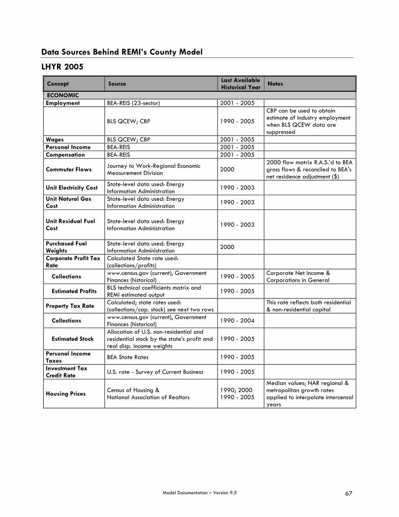
Model Documentation – Version 9.5 67
Data Sources Behind REMI’s County Model
LHYR 2005
Concept Source Last Available Historical Year Notes
ECONOMIC Employment BEA-REIS (23-sector) 2001 - 2005
BLS QCEW; CBP 1990 - 2005
CBP can be used to obtain estimate of industry employment when BLS QCEW data are suppressed
Wages BLS QCEW; CBP 2001 - 2005 Personal Income BEA-REIS 2001 - 2005 Compensation BEA-REIS 2001 - 2005
Commuter Flows Journey to Work-Regional Economic Measurement Division 2000
2000 flow matrix R.A.S.’d to BEA gross flows & reconciled to BEA's net residence adjustment ($)
Unit Electricity Cost State-level data used: Energy Information Administration 1990 - 2003
Unit Natural Gas Cost
State-level data used: Energy Information Administration 1990 - 2003
Unit Residual Fuel Cost
State-level data used: Energy Information Administration 1990 - 2003
Purchased Fuel Weights
State-level data used: Energy Information Administration 2000
Corporate Profit Tax Rate
Calculated State rate used: (collections/profits)
Collections www.census.gov (current), Government Finances (historical) 1990 - 2005 Corporate Net Income &
Corporations in General
Estimated Profits BLS technical coefficients matrix and REMI estimated output 1990 - 2005
Property Tax Rate Calculated; state rates used: (collections/cap. stock) see next two rows This rate reflects both residential
& non-residential capital
Collections www.census.gov (current), Government Finances (historical) 1990 - 2004
Estimated Stock Allocation of U.S. non-residential and residential stock by the state’s profit and real disp. income weights
1990 - 2005
Personal Income Taxes BEA State Rates 1990 - 2005
Investment Tax Credit Rate U.S. rate - Survey of Current Business 1990 - 2005
Housing Prices Census of Housing & National Association of Realtors
1990; 2000 1990 - 2005
Median values; NAR regional & metropolitan growth rates applied to interpolate intercensal years
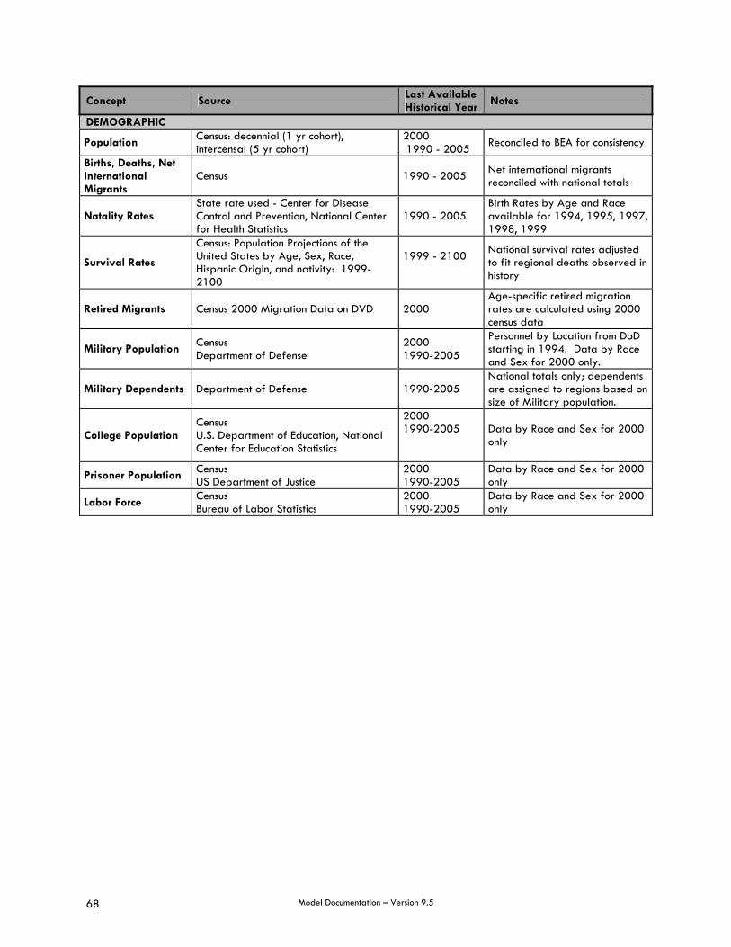
Model Documentation – Version 9.5 68
Concept Source Last Available Historical Year Notes
DEMOGRAPHIC
Population Census: decennial (1 yr cohort), intercensal (5 yr cohort)
2000 1990 - 2005 Reconciled to BEA for consistency
Births, Deaths, Net International Migrants
Census 1990 - 2005 Net international migrants reconciled with national totals
Natality Rates State rate used - Center for Disease Control and Prevention, National Center for Health Statistics
1990 - 2005
Birth Rates by Age and Race available for 1994, 1995, 1997, 1998, 1999
Survival Rates
Census: Population Projections of the United States by Age, Sex, Race, Hispanic Origin, and nativity: 1999-2100
1999 - 2100
National survival rates adjusted to fit regional deaths observed in history
Retired Migrants Census 2000 Migration Data on DVD 2000 Age-specific retired migration rates are calculated using 2000 census data
Military Population Census Department of Defense
2000 1990-2005
Personnel by Location from DoD starting in 1994. Data by Race and Sex for 2000 only.
Military Dependents Department of Defense 1990-2005 National totals only; dependents are assigned to regions based on size of Military population.
College Population Census U.S. Department of Education, National Center for Education Statistics
2000 1990-2005
Data by Race and Sex for 2000 only
Prisoner Population Census US Department of Justice
2000 1990-2005
Data by Race and Sex for 2000 only
Labor Force Census Bureau of Labor Statistics
2000 1990-2005
Data by Race and Sex for 2000 only
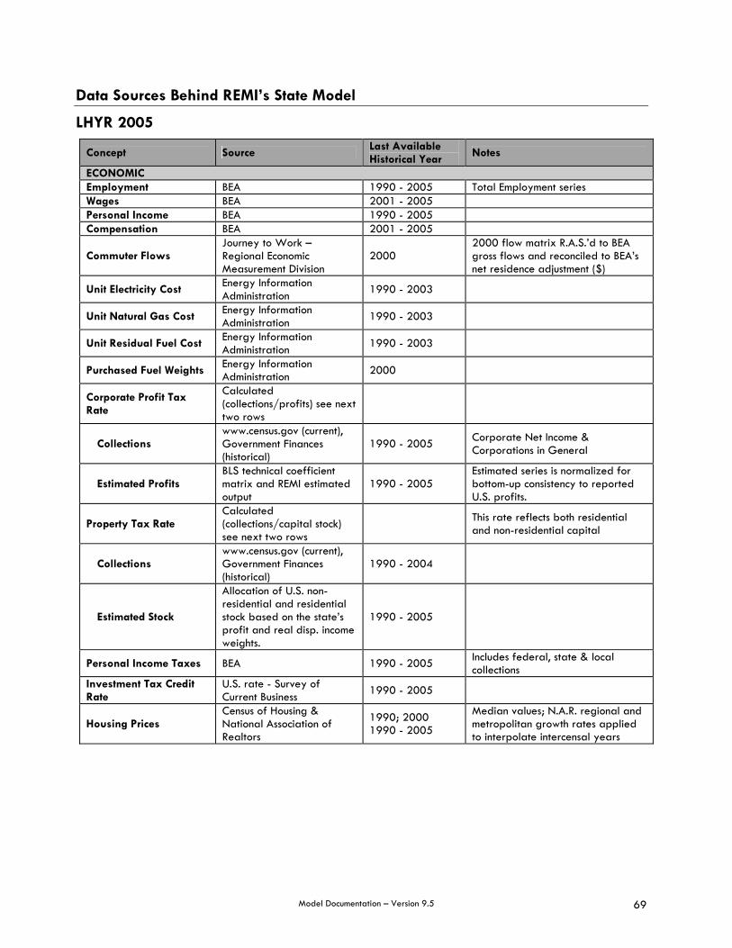
Model Documentation – Version 9.5 69
Data Sources Behind REMI’s State Model
LHYR 2005
Concept Source Last Available Historical Year Notes
ECONOMIC Employment BEA 1990 - 2005 Total Employment series Wages BEA 2001 - 2005 Personal Income BEA 1990 - 2005 Compensation BEA 2001 - 2005
Commuter Flows Journey to Work – Regional Economic Measurement Division
2000 2000 flow matrix R.A.S.’d to BEA gross flows and reconciled to BEA’s net residence adjustment ($)
Unit Electricity Cost Energy Information Administration 1990 - 2003
Unit Natural Gas Cost Energy Information Administration 1990 - 2003
Unit Residual Fuel Cost Energy Information Administration 1990 - 2003
Purchased Fuel Weights Energy Information Administration 2000
Corporate Profit Tax Rate
Calculated (collections/profits) see next two rows
Collections www.census.gov (current), Government Finances (historical)
1990 - 2005 Corporate Net Income & Corporations in General
Estimated Profits BLS technical coefficient matrix and REMI estimated output
1990 - 2005 Estimated series is normalized for bottom-up consistency to reported U.S. profits.
Property Tax Rate Calculated (collections/capital stock) see next two rows
This rate reflects both residential and non-residential capital
Collections www.census.gov (current), Government Finances (historical)
1990 - 2004
Estimated Stock
Allocation of U.S. non-residential and residential stock based on the state’s profit and real disp. income weights.
1990 - 2005
Personal Income Taxes BEA 1990 - 2005 Includes federal, state & local collections
Investment Tax Credit Rate
U.S. rate - Survey of Current Business 1990 - 2005
Housing Prices Census of Housing & National Association of Realtors
1990; 2000 1990 - 2005
Median values; N.A.R. regional and metropolitan growth rates applied to interpolate intercensal years
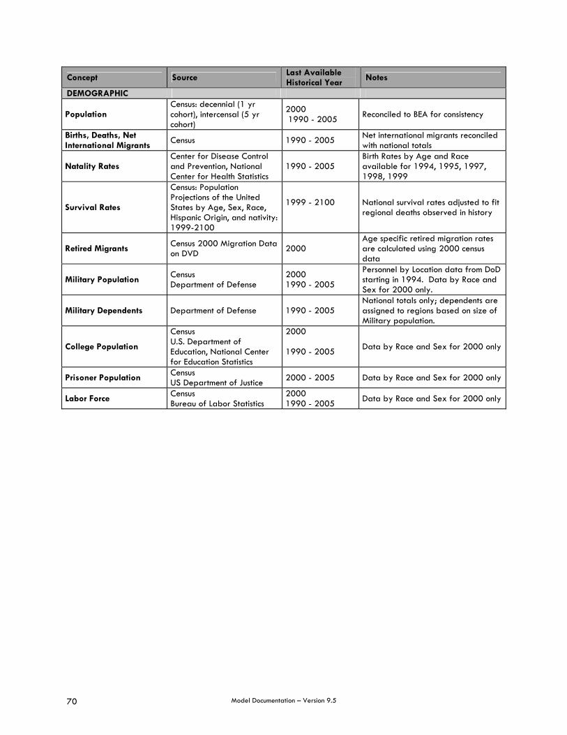
Model Documentation – Version 9.5 70
Concept Source Last Available Historical Year Notes
DEMOGRAPHIC
Population Census: decennial (1 yr cohort), intercensal (5 yr cohort)
2000 1990 - 2005 Reconciled to BEA for consistency
Births, Deaths, Net International Migrants Census 1990 - 2005 Net international migrants reconciled
with national totals
Natality Rates Center for Disease Control and Prevention, National Center for Health Statistics
1990 - 2005
Birth Rates by Age and Race available for 1994, 1995, 1997, 1998, 1999
Survival Rates
Census: Population Projections of the United States by Age, Sex, Race, Hispanic Origin, and nativity: 1999-2100
1999 - 2100
National survival rates adjusted to fit regional deaths observed in history
Retired Migrants Census 2000 Migration Data on DVD 2000
Age specific retired migration rates are calculated using 2000 census data
Military Population Census Department of Defense
2000 1990 - 2005
Personnel by Location data from DoD starting in 1994. Data by Race and Sex for 2000 only.
Military Dependents Department of Defense 1990 - 2005 National totals only; dependents are assigned to regions based on size of Military population.
College Population
Census U.S. Department of Education, National Center for Education Statistics
2000 1990 - 2005
Data by Race and Sex for 2000 only
Prisoner Population Census US Department of Justice 2000 - 2005 Data by Race and Sex for 2000 only
Labor Force Census Bureau of Labor Statistics
2000 1990 - 2005 Data by Race and Sex for 2000 only

Model Documentation – Version 9.5 71
Data Sources Behind REMI’s U.S. Model
LHYR 2005
Concept Source Last Available Historical Year Notes
ECONOMIC Employment BEA 1990 - 2005 Total Employment series Wages BEA 2001 - 2005 Personal Income BEA 1990 - 2005 Compensation BEA 2001 - 2005
Occupational Matrix BLS 2004; 2014 Details 94 occupations, linearly interpolated
Productivity BLS 1998 - 2004; 2014
Calculated from detailed E & Q data
Technology Matrix BLS 1998 - 2004; 2014
Make & Use matrices converted to industry-by-industry matrices. Interpolated for in-between years.
Industry Deflators BLS 1998 - 2004 Nominal & real Q to calculate deflators
Final Demand BLS 1998 - 2004; 2014
Interpolated by growth in labor force for in-between years.
Commodity Prices Survey of Current Business: NIPA 1990 - 2005
Unit Electricity Cost Energy Information Administration 1990 - 2003
Unit Natural Gas Cost Energy Information Administration 1990 - 2003
Unit Residual Fuel Cost Energy Information Administration 1990 - 2003
Purchased Fuel Weights Energy Information Administration 2000
Corporate Profit Tax Rate
Calculated (collections/profits) see next two rows
Collections www.census.gov (current), Government Finances (historical)
1990 - 2005 Corporate Net Income & Corporations in General
Profits Survey of Current Business 1990 - 2005 Moving average to convert from fiscal year to calendar year.
Property Tax Rate Calculated (collections/capital stock) see next 2 rows
This rate reflects both residential & non-residential capital
Collections www.census.gov (current), Government Finances (historical)
1990 - 2005
Estimated Stock Survey of Current Business 1990 - 2005
Personal Income Taxes BEA 1990 - 2005 Includes federal, state & local collections
Investment Tax Credit Rate Survey of Current Business 1990 - 2005
Business Cycle RSQE 2006 - 2008
Housing Prices Census of Housing & National Association of Realtors
1990; 2000 1990 - 2005

Model Documentation – Version 9.5 72
Concept Source Last Available Historical Year Notes
DEMOGRAPHIC Population Census: (1 yr. cohort) 1990 - 2005 Reconciled to BEA for consistency Births, Deaths, Net International Migration
Census 1990 - 2005
Natality Rate, Survival Rate, Net International Migration Forecasts
Census: Population projections of the United States by Age, Sex, Race, Hispanic Origin, and Nativity
1999 - 2100
Labor Force BLS 1990 - 2005 Labor Force Participation Rates Forecast
BLS 2000 - 2050
Military Population Census; Department of Defense
2000; 1990 - 2005
Military Dependents Department of Defense 1990 - 2005
College Population U.S. Department of Education; National Center for Education Statistics
1990 - 2005
Prisoner Population Census; U.S. Department of Justice
2000; 1990 - 2005

Model Documentation – Version 9.5 73
Chapter 4: Chained vs. Fixed Real Dollars in the REMI Model
In 1995 the Bureau of Economic Analysis (BEA) introduced new measures of real output and prices which are calculated using chain-type annual-weighted indexes, allowing for the effects of changes in relative prices and changes in the composition of output over time. The previous use of fixed-weighted measures for periods other than those close to the base period resulted in a “substitution bias” that caused an overstatement of growth for periods after the base year and an understatement for periods before the base year. The computer sector, with its rapidly declining prices and increasing output, provides a clear example of the benefit of using a chain-weighted measure rather than a fixed-weighted measure. The use of fixed (single year) weights significantly overstates the impact of recent investment in computers in relation to investment in other types of assets, especially as one gets farther away from the weighting period, because the prices are dropping so quickly. Shifting the valuations on a year-by-year basis allows long-term growth, past business cycles, and productivity to be measures in the valuations that are appropriate to the period being studied4.
The REMI model relies on national input-output relationships reported by the BLS. These relationships, since they are at the most “detailed” level, are provided in fixed real dollars. However, the BEA reports Gross Domestic Product (GDP) and its aggregate final demand components in chained real dollars. To reconcile these two sets of variables, REMI has implemented the following methodology:
1. All real dollar concepts used in the model are based on fixed weights. This allows the industry value added and final demand totals to remain balanced, and allows us to use the input-output tables, aggregated to either 23, 70, or 169 sectors, as reported by the BLS. Fixed dollar GDP/GRP concepts are obtained for history and for the year currently projected by aggregating the detailed series reported by the BLS. The model then predicts all of the other forecast years.
2. An alternative GDP/GRP table reporting chain-weighted dollars has been added to the Results tab. To generate this series, we first predict the relative prices for each industry. For history, these relative prices equal the industry deflators reported by the BLS. For forecasts, they are based on the change in the industry wage rate relative to the change in industry productivity5, and become the industry deflators
4 “Preview of the Comprehensive Revision of the National Income and Product Accounts: BEA’s New Featured Measures of Output and Prices,”
Survey of Current Business (July 1995): 31-38.
5 T
iTTtt
Ti
Ti
ti
ti
T
tt
i DEFPRODWRPRODWRPRODWRPRODWR
CPICPIP ∗∗=
))/()(())()((
where,
=iP relative price (deflator) for industry i
=CPI consumer price index
=iWR wage rate for industry i
=WR wage rate for economy
=iPROD labor productivity for industry i
=PROD labor productivity for economy
=iDEF deflator for industry I

Model Documentation – Version 9.5 74
reported in the model. Starting in 2001, we then use these relative prices to generate nominal dollar series for the detailed final demand components, and apply a chain-weighting methodology6 to estimate the chained dollar values. Since the BLS reports actual chained dollar values for history and for their projected year, we are able to normalize our estimated series to the actual values for these years. The normalization “ratios” are carried forward into the forecast for the purpose of consistency.
3. All user inputs for the aggregated final demand components (e.g. Macroeconomic Values tab and policy variables) will be entered in chained real dollars, with the exception of the final demand translators, which, since they are available at the disaggregate level, will be entered in fixed real dollars. All user inputs for the industry-level policy variables will be entered in fixed real dollars.
=t current year
T = last history year
6 1
1,
, −− ∗
∗
∗=
∑∑ t
jtji
ti
tji
tit
j FDCFDFPFDFP
FDC
where,
=jFDC chained real dollar final demand for component j
=jiFDF , fixed real dollar final demand for component j in industry i
=iP relative price (deflator) for industry i
=t current time period
=−1t previous time period

Model Documentation – Version 9.5 75
Chapter 5: State And Local Government Employment And Final Demand
(May 2000) The Bureau of Economic Analysis (BEA) reports state government employment separate from local government employment at the county level for all history years beginning in 1979. In addition to now providing this detail on the Results tab in Policy Insight, we are also using this data to distribute state and local final demand to its separate state and local shares over this same period of history. All of this information together allows us to predict state government employment and final demand separately from local demand for the forecast period. The methodology we implemented is based on the following basic assumptions:
1. State and local government labor productivity is the same (as the U.S.) in all counties for all state and local government employees anywhere, whether state or local7.
2. Final per capita demand for state government employees is different by state but not by local area within a state.
3. Final per capita demand for local government employees is different for each local area (k). 4. Local government demand is always met by the local government in area k, but state government
demand is not always met by the state government in local area k. This is because state government employees are usually centralized within a few local areas in a state instead of being distributed throughout the state.
U.S. Model
For the U.S. model history, state government final demand is split from the BEA-reported state and local government final demand based on the BEA-reported state government employment as a share of state and local government employment. An analogous approach is used for estimating local government final demand.
FDust,t = (Eust,t/Eustloc,t) * FDustloc,t
FDuloc,t = (Euloc,t/Eustloc,t) * FDustloc,t
where,
FDust,t = state government final demand for the U.S. in year t Eust,t = state government employment for the U.S. in year t, as reported by the BEA Eustloc,t = state and local government employment for the U.S. in year t, as reported by the BEA FDustloc,t = state and local government final demand for the U.S. in year t, as reported by the BEA Euloc,t = local government employment for the U.S. in year t, as reported by the BEA
7 (Ekstloc,t / FDkstloc,t) = (Eustloc,t / FDustloc,t)
where, Ekstloc,t = state and local government employment in local area k in year t FDkstloc,t = state and local government final demand in local area k in year t Eustloc,t = state and local government employment in the U.S. in year t FDustloc,t = state and local government final demand in the U.S. in year t
Model Documentation – Version 9.5 76
FDuloc,t = local government final demand for the U.S. in year t
For the U.S. model forecast, state government final demand is split from the predicted state and local government final demand based on the last history year ratio of state government employment to state and local government employment. An analogous approach is used for predicting local government final demand.
FDust,t = (Eust,T / Eustloc,T) * FDustloc,t
FDuloc,t = (Euloc,T / Eustloc,T) * FDustloc,t
where
Eust,T = state government employment for the U.S. in the last history year, as reported by the BEA Eustloc,T = state and local government employment for the U.S. in the last history year, as reported by
the BEA FDustloc,t = state and local government final demand for the U.S. in year t, as predicted by the REMI
model Euloc,T = local government employment for the U.S. in the last history year, as reported by the BEA
State government employment is split from the predicted state and local government employment based on the predicted state government final demand as a share of predicted state and local government final demand.
Eust,t = (FDust,t/FDustloc,t) * Eustloc,t
Euloc,t = (FDuloc,t/FDustloc,t) * Eustloc,t
where
Eust,t = state government employment for the U.S. in year t Eustloc,t = state and local government employment for the U.S. in year t, as predicted by the REMI
model Euloc,t = local government employment for the U.S. in year t
State Models
For a state model history, state government final demand is estimated by applying the state and local government final demand per state and local government employee in the U.S. to the BEA-reported state government employment in the state. An analogous approach is used for estimating local government final demand.
FDsst,t = (FDustloc,t / Eustloc,t) * Esst,t
FDsloc,t = (FDustloc,t / Eustloc,t) * Esloc,t
where,
FDsst,t = state government final demand for the state in year t Esst,t = state government employment for the state in year t, as reported by the BEA Eustloc,t = state and local government employment for the U.S. in year t, as reported by the BEA
Model Documentation – Version 9.5 77
FDustloc,t = state and local government final demand for the U.S. in year t, as reported by the BEA FDsloc,t = local government final demand for the state in year t Esloc,t = local government employment for the state in year t, as reported by the BEA
For a state model forecast, state government final demand is predicted based on the state government final demand spending per person in the state in the last history year, the change in the state and local government spending per person in the U.S. relative to the last history year, and the state’s current year population. An analogous approach is used for predicting local government final demand.
FDsst,t = (FDsst,T / NsT) * ((FDustloc,t / Nut) / (FDustloc,T / NuT)) * Nst
FDsloc,t = (FDsloc,T / NsT) * ((FDustloc,t / Nut) / (FDustloc,T / NuT)) * Nst
where
FDsst,T = state government final demand for the state in the last history year, as estimated by the REMI model
NsT = total population for the state in the last history year, as reported by the BEA Nut = total population for the U.S. in year t, as predicted by the REMI model NuT = total population for the U.S. in the last history year, as reported by the BEA Nst = total population for the state in year t, as predicted by the REMI model FDsloc,T = local government final demand for the state in the last history year, as estimated by the
REMI model
State government employment is predicted by applying the state and local government employment per dollar of state and local government final demand in the U.S. to the predicted state government final demand in the state. An analogous approach is used for predicting local government employment.
Esst,t = (Eustloc,t / FDustloc,t) * FDsst,t
Esloc,t = (Eustloc,t / FDustloc,t) * FDsloc,t
County Models
For a county model history, state government final demand is estimated by applying the state government final demand per person in the state to the BEA reported total population in the local area.
FDkst,t = (FDs
st,t / Nst) * Nk
t where
FDkst,t = state government final demand for local area k in year t Nkt = total population for local area k in year t, as reported by the BEA
Local government final demand is estimated by applying the state and local government final demand per state and local government employee in the U.S. to the BEA-reported local government employment in the local area.
FDkloc,t = (FDustloc,t / Eustloc,t) * Ekloc,t
where
Model Documentation – Version 9.5 78
FDkloc,t = local government final demand for local area k in year t Ekloc,t = local government employment for local area k in year t, as reported by the BEA
For a county model forecast, state government final demand is predicted based on the state government final demand spending per person in the state in the last history year, the change in the state and local government spending per person in the U.S. relative to the last history year, and the local area’s current year population.
FDkst,t = (FDsst,T / NsT) * ((FDustloc,t / Nut) / (FDustloc,T / NuT)) * Nkt
Local government final demand is predicted based on the local government final demand spending per person in the local area in the last history year, the change in the state and local government spending per person in the U.S. relative to the last history year, and the local area’s current year population.
FDkloc,t = (FDkloc,T / NkT) * ((FDustloc,t / Nut) / (FDustloc,T / NuT)) * Nkt
For a single-region model, state government employment is predicted based on the assumption that if the number of employees per dollar of final demand in the local area equals or exceeds the state average in the last history year, then the proportion of local demand supplied locally is set equal to one and the additional output is an export from that county. An example of this is a county where the state capital is located. Likewise, if the number of employees per dollar of final demand in the local area is less than the state average in the last history year, then the proportion of local demand supplied locally is less than one, leading to less local employment than the local demand for state services would, on its own, suggest.
RPCkst,T = ((FDsstloc,T / Esstloc,T) * Ekst,T ) / FDkst,T
EXPkst,t = ((Ekst,T – (FDkst,T * (Esstloc,T / FDsstloc,T))) / Eust,T ) * Eust,t
If RPC < 1 Ekst,t = (Esstloc,t / FDsstloc,t) * RPCst,T * FDkst,t
If RPC = 1 Ekst,t = ((Esstloc,t / FDsstloc,t) * FDkst,t) + EXPkst,t
where
RPCkst,T = proportion of the local demand that is supplied locally for local area k in the last history year
EXPkst,t = amount of state government employment in local area k based on demand from outside of local area k
For a multiregion model, state government employment is predicted based on the assumption that there is state government “trade” that flows between the regions. Some regions “export” state government employees (e.g. counties where a state capital is located) while other regions “import” state government employees.
EXPMRkst,t = Σ(kfsT * IMPMRlst,t)
If all regions are in one state kfsT = EXPMRkst,T / ΣIMPMRlst,T
where l є s and ΣIMPMRlst,T = sum of imports for all counties in the state
If a multi-county model when k and g are not in the same state kfgT = 0

Model Documentation – Version 9.5 79
If positive EXPMRkst,T =((FDsstloc,T / Esstloc,T) * Ekst,T) - FDkst,T
If negative EXPMRkst,T = 0
If positive IMPMRlst,T = ((FDsst,T / NsT) * NlT) - ((FDsstloc,T / Esstloc,T) * Elst,T)
If negative IMPMRlst,T = 0
If positive IMPMRlst,t = FDkst,t - (((FDsstloc,T/Esstloc,T)*((FDustloc,t/Eustloc,t)/(FDustloc,T/Eustloc,T))*Ekst,t)
If negative IMPMRlst,t = 0
If RPC < 1 Ekst,t = (Esstloc,t / FDsstloc,t) * RPCkst,T * FDkst,t
If RPC = 1 Ekst,t = ((Esstloc,t / FDsstloc,t) * FDkst,t) + (EXPMRkst,t * (Esstloc,t/FDsstloc,t))
where,
EXPMRkst,t = amount of state government in local area k attributable to demand in the other model regions, for time period t
kfsT = state government “trade flow” coefficient for local area k within a state s, for the last history year
IMPMRlst,t = amount of state government that local area l (where l є s) demands but is not able to supply, in time period t
Local government employment is predicted by applying the state and local government employment per dollar of state and local government final demand in the U.S. to the predicted local government final demand in the local area.
Ekloc,t = (Esstloc,t / FDsstloc,t) * FDkloc,t
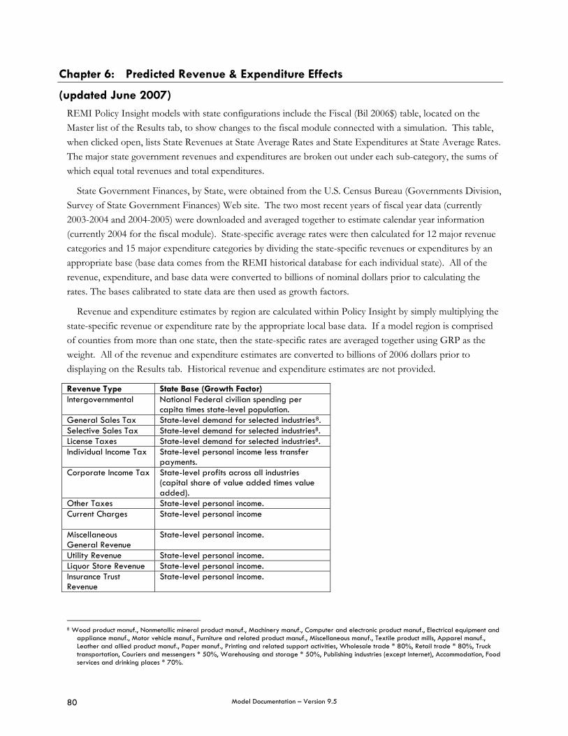
Model Documentation – Version 9.5 80
Chapter 6: Predicted Revenue & Expenditure Effects
(updated June 2007) REMI Policy Insight models with state configurations include the Fiscal (Bil 2006$) table, located on the Master list of the Results tab, to show changes to the fiscal module connected with a simulation. This table, when clicked open, lists State Revenues at State Average Rates and State Expenditures at State Average Rates. The major state government revenues and expenditures are broken out under each sub-category, the sums of which equal total revenues and total expenditures.
State Government Finances, by State, were obtained from the U.S. Census Bureau (Governments Division, Survey of State Government Finances) Web site. The two most recent years of fiscal year data (currently 2003-2004 and 2004-2005) were downloaded and averaged together to estimate calendar year information (currently 2004 for the fiscal module). State-specific average rates were then calculated for 12 major revenue categories and 15 major expenditure categories by dividing the state-specific revenues or expenditures by an appropriate base (base data comes from the REMI historical database for each individual state). All of the revenue, expenditure, and base data were converted to billions of nominal dollars prior to calculating the rates. The bases calibrated to state data are then used as growth factors.
Revenue and expenditure estimates by region are calculated within Policy Insight by simply multiplying the state-specific revenue or expenditure rate by the appropriate local base data. If a model region is comprised of counties from more than one state, then the state-specific rates are averaged together using GRP as the weight. All of the revenue and expenditure estimates are converted to billions of 2006 dollars prior to displaying on the Results tab. Historical revenue and expenditure estimates are not provided.
Revenue Type State Base (Growth Factor) Intergovernmental National Federal civilian spending per
capita times state-level population. General Sales Tax State-level demand for selected industries8. Selective Sales Tax State-level demand for selected industries8. License Taxes State-level demand for selected industries8. Individual Income Tax State-level personal income less transfer
payments. Corporate Income Tax State-level profits across all industries
(capital share of value added times value added).
Other Taxes State-level personal income. Current Charges
State-level personal income
Miscellaneous General Revenue
State-level personal income.
Utility Revenue State-level personal income. Liquor Store Revenue State-level personal income. Insurance Trust Revenue
State-level personal income.
8 Wood product manuf., Nonmetallic mineral product manuf., Machinery manuf., Computer and electronic product manuf., Electrical equipment and
appliance manuf., Motor vehicle manuf., Furniture and related product manuf., Miscellaneous manuf., Textile product mills, Apparel manuf., Leather and allied product manuf., Paper manuf., Printing and related support activities, Wholesale trade * 80%, Retail trade * 80%, Truck transportation, Couriers and messengers * 50%, Warehousing and storage * 50%, Publishing industries (except Internet), Accommodation, Food services and drinking places * 70%.
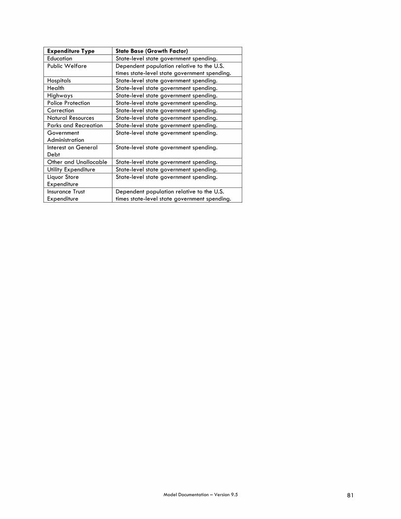
Model Documentation – Version 9.5 81
Expenditure Type State Base (Growth Factor) Education State-level state government spending. Public Welfare Dependent population relative to the U.S.
times state-level state government spending. Hospitals State-level state government spending. Health State-level state government spending. Highways State-level state government spending. Police Protection State-level state government spending. Correction State-level state government spending. Natural Resources State-level state government spending. Parks and Recreation State-level state government spending. Government Administration
State-level state government spending.
Interest on General Debt
State-level state government spending.
Other and Unallocable State-level state government spending. Utility Expenditure State-level state government spending. Liquor Store Expenditure
State-level state government spending.
Insurance Trust Expenditure
Dependent population relative to the U.S. times state-level state government spending.

Model Documentation – Version 9.5 82
Chapter 7: Using the Fiscal Module in REMI Policy Insight
Introduction This chapter provides a conceptual framework, along with a step-by-step procedure, for using the fiscal module in Policy Insight. REMI developed the fiscal module as a convenient tool for tabulating the fiscal impacts of policies being simulated in the economic model. To use the fiscal module properly, you must understand how to calibrate the baseline forecast to reflect actual budgeted revenue and expenditure levels, and how to ensure that the forecasted fiscal results capture all of the policy’s impacts (including direct and indirect effects). This chapter presents the current approach to obtaining fiscal results that complement the model’s economic outputs. Please note that the fiscal module is only available in models that include at least one entire state.
Theory and Methodology Policy Insight essentially consists of two sequential components: an economic engine that produces simulations of economic and demographic effects, and a fiscal module that runs subsequent to the simulation for bookkeeping purposes. To understand the full economic and fiscal impacts of a proposed policy change, analysts must use both components. For example, to simulate an increase in the equipment tax, analysts must first capture the economic shock through changes to economic policy variables--specifically, an increased equipment tax rate and increased government spending (if any) due to the incremental tax revenues. The simulation then measures the indirect and induced effects produced by the initial economic shock. Following the economic simulation, the impact on tax revenues is factored into the fiscal module to capture the expected static change in baseline receipts for the relevant tax category. Next, the increased government spending (if any) facilitated by the additional revenue is entered into fiscal-module expenditures, broken down by spending category. Both these stages may require calibration to ensure that fiscal results in Policy Insight match the user’s projections.
In Policy Insight, “economic” government spending (the policy variable) and “fiscal” government expenditures are defined differently. The government-spending policy variable is designed to capture only those governmental outlays that contribute directly to gross regional product (GRP). By contrast, government spending oriented toward non-productive ends (such as debt service and the redistribution of income) count as budget entries in the fiscal module, but should not be factored into the government-spending economic policy variable. Because of this disparity, quantities entered into the government-spending policy variable and fiscal expenditures may be different.
Baseline Calibration Before beginning the simulation process, you should calibrate Policy Insight’s baseline fiscal revenues and expenditures in the initial forecast year so that the values are consistent with available actual calendar-year tax receipts and line-item budget data. REMI derives its fiscal segment ratios from Census Bureau data, based on a census of governments conducted at five-year intervals, and an annual survey for the intervening years. REMI averaged census data from the most recent two fiscal years to create calendar-year ratios, which were applied to the historical data from the model’s last history year. Because of the data publication lag, the tax activity of legislatures, and the more frequent release of such information within certain political jurisdictions (state, etc.), Policy Insight must be recalibrated to reflect current state data. This fiscal variable calibration

Model Documentation – Version 9.5 83
process is external to the model; it only affects bookkeeping of fiscal revenues and expenditures, leaving REMI policy variables unchanged. For this reason, you must calibrate the fiscal module only after entering and running all other control forecast adjustments.
First, open the standard regional control (or the adjusted regional control if a new benchmark has been created) and switch to the Results tab. Scroll down to the bottom of the results list to examine the two Fiscal tables (which consist of state revenues and expenditures by category) to determine the existence and magnitude of any discrepancies in the initial year between the model’s data and the user’s information. The simplest method is to copy the first-year figures into a spreadsheet and calculate percentage differences between model and user data for each revenue or expenditure category from your own static projections. The table below lists the fiscal variables in which discrepancies may arise.
Revenue Fiscal Variables Expenditure Fiscal Variables
Intergovernmental Education
General Sales Tax Public Welfare
Selective Sales Tax Hospitals
License Taxes Health
Individual Income Tax Highways
Corporate Income Tax Police Protection
Other Taxes Correction
Current Charges Natural Resources
Miscellaneous General Revenue Parks and Recreation
Utility Revenue Government Administration
Liquor Store Revenue Interest on General Debt
Insurance Trust Revenue Other and Unallocable
Utility Expenditure
Liquor Store Expenditure
Insurance Trust Expenditure
You should first convert your data to 2006 constant dollars to be consistent with the units of the fiscal module information. You may also need to transform fiscal-year data into the calendar-year data used by REMI, which can be accomplished by summing two consecutive fiscal years’ values and dividing the result by two.
Next, create a new Regional Control using the File menu. If you want to use an adjusted regional control as the base, then open the adjusted regional control and edit that. Go to the Policy Variable Selection tab and select fiscal variables from the Fiscal Calibration category for each revenue/expenditure category for which a discrepancy exists. In the Policy Variable Values tab, enter the computed percentage deviations into the corresponding variables for all years of the forecast, by pasting values from the spreadsheet. To enter fiscal calibration changes for input units set to Proportion, calculate fiscal inputs as user values minus REMI values, divided by REMI values. To enter fiscal calibration changes for input units set to Percent (default input units), calculate fiscal inputs as the user values minus REMI values, divided by REMI values, then multiplied by 100 to generate input changes as percentages. If the user value for a fiscal category exceeds the
Model Documentation – Version 9.5 84
corresponding REMI value, then input the fiscal variable adjustment as positive; if the user value is less than the REMI value, input the adjustment as negative.
The adjustment must be applied to all years equally in percentage terms, since fiscal forecasts build off their respective base years, which diverged by a known percentage. For example, if state general sales tax revenues are low by 3.5% in the first year, enter 3.5% into all years for the State/General Sales Tax fiscal calibration policy variable. You may also calculate fiscal adjustment inputs for more than one forecast calendar year, if you have two years of historical data beyond those contained in Policy Insight. In that case, to apply an adjustment through the last forecast year, you must either average the calendar years for which you have calculated input adjustments, or decide which year’s adjustment is the best candidate to apply through the last forecast year. Once this percentage adjustment has been implemented, any future movement in the revised fiscal forecast represents indirect effects of endogenous processes in the economic model, such as population shifts.
Running Simulations In developing simulations, the most suitable policy variables for analyzing effects depend on the nature of the policy change being evaluated. To model a tax policy, you may be able to use a tax rate policy variable such as the Equipment Tax Rate or Corporate Profit Tax Rate. In cases where these variables are not suitable for the analysis, you must “disguise” the effect of the tax as an economic concept before incorporating it in the economic model. For example, an increased property tax rate would be entered as an increase in housing prices based on a static tax amount calculated as some percentage multiplied by the residential capital stock. An increased tax on a particular type of capital equipment might be entered as either an increased cost of capital or an increased cost of production for the sectors that utilize that equipment. An increase in a sales tax on a consumer commodity might be entered either as a point change in the sales tax or as a static change (after allowing for price elasticity effects on quantity demanded of the commodity) in the tax amount to be collected.
When applying fiscal variables to simulations, insert fiscal variable entries to track tax-related or government spending-related policy variable entries starting from the calendar year in which the fiscal shock occurs in the policy simulation. Then, carry the policy variable and fiscal variable entries for the tax or spending shock in the simulation through the last forecast year, or through the sunset year of the shock, whichever is sooner.
In the simulation mode, when using fiscal variables as well as economic policy variables, only one model run is required to properly process the policy variables together with the fiscal variables. However, when creating the simulation, remember in the Forecast Selection Tab to specify the new control file containing the adjusted baseline fiscal data.
Example For the example of an equipment tax hike, there are three direct effects we must incorporate into the model. In the economic model, we need to address both the higher equipment tax and the increased governmental spending (if any) that draws from the incremental equipment tax revenues. The third effect involves the post-simulation fiscal balance, which we must restore by adjustments to government tax revenues and expenditures.

Model Documentation – Version 9.5 85
First, for the industrial and commercial sectors, if the tax applies to the full spectrum of equipment, we can model the tax hike using the Equipment Tax Rate policy variable. Increasing this rate will translate into a higher cost of capital and induce substitution away from capital, thereby increasing labor intensities of production.
Second, if the tax is being increased to fund net new spending, we can allocate the increase in government spending to different economic sectors if the funds are earmarked for a specific purpose. If the tax is being increased to cover an operating deficit and thereby merely maintain existing spending, then no spending variables are involved. For example, if incremental tax revenues will be spent on transportation or education, then we can shock the corresponding policy variables. Alternatively, if the government plans on redistributing the income, the analyst could manipulate policy variables involving transfer payments to individuals. In the absence of such specific information, the increase may simply be entered into the “Government Spending-State” policy variable, which allocates those monies primarily to government payroll and to construction. Remember, however, that the expenditure amount and allocation entered into the fiscal module will likely vary from the policy variable amount, because of their different compositions.
Finally, after running the economic simulation, the analyst should input tax revenues (based on static projections) and expenditures into the fiscal tracking module. Model the additional equipment tax revenue as receipts under the most suitable tax category (such as “State General Sales Tax Revenue”), and allocate the associated expenditures across categories (such as education and health) based on either general priorities or specifically known earmarkings of the incremental funds. A second round of calibration (as described above) may be required to align the initial-year forecasts of revenues and expenditures with the user’s static projections. Once these percentage adjustments are entered across the full forecast period, remaining differences relative to the static forecast must reflect indirect effects stemming from predicted economic and demographic dynamics.
Model Documentation – Version 9.5 86
Chapter 8: Decomposing Policy Effects On Employment, Wages, And Prices By Income Groups
June 2007 A table entitled “Percentage Changes from Control Forecast by Quintiles” is generated for evaluating the economic impacts of policies on different compensation and income groups. This documentation discusses the industry and occupation classifications, the economic background, and the operation of this procedure.
Industrial Classification
Annual average U.S. compensation rates for 66 private non-farm sectors are obtained for 2005 from the BEA employment and compensation series. The compensation rates are ranked in ascending order and then divided into five equal groups. The ranges of annual average compensation rates for the five industry groups are listed below:
Range of Industrial Compensation Rates Group 1 (First 20%) $6,799 – $24,701 Group 2 (Second 20%) $27,233 - $42,835 Group 3 (Third 20%) $44,194 - $53,840 Group 4 (Fourth 20%) $55,674 - $68,643 Group 5 (Fifth 20%) $69,373 - $118,718
Occupational Classification
Median weekly U.S. wage rates for 94 occupations are obtained from the 2005 BLS Employment and Earnings. The wage rates are ranked in ascending order, and then divided into five groups. The ranges of occupational wage rates are listed below:
Range of Occupational Wage Rates Group 1 (First 20%) $336 - $456 Group 2 (Second 20%) $466 - $585 Group 3 (Third 20%) $604 - $734 Group 4 (Fourth 20%) $740 - $890 Group 5 (Fifth 20%) $920 - $1834
Personal Expenditure Classification
Average annual expenditures for consumers by quintiles or by ranges of income are obtained from the 2005 BLS Consumer Expenditure Survey. The eight income ranges are as follows:
Group Range 1 <$5,000 2 $5,000-$9,999 3 $10,000-$14,999 4 $15,000-$19,999 5 $20,000-$29,999 6 $30,000-$39,999 7 $40,000-$49,999 8 $50,000+
Economic Background
The percentage changes from control forecasts for industrial and occupational compensation rates and employment are reported on the table. Note that the simulation (alternative) forecast must be generated before running the software. For each item, the percentage change is calculated as follows:
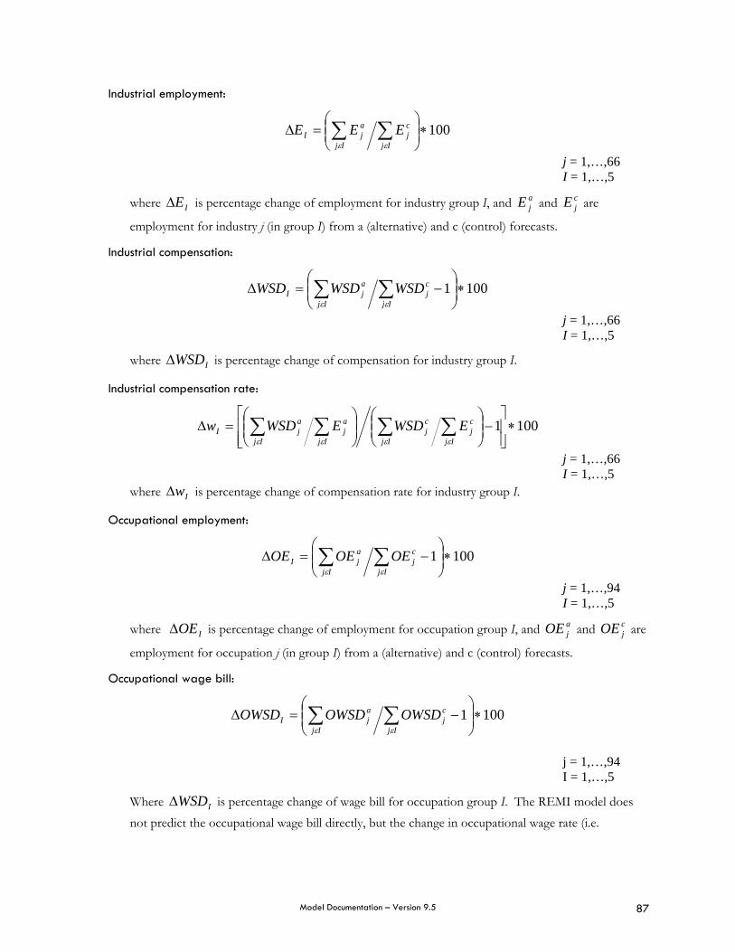
Model Documentation – Version 9.5 87
Industrial employment:
100∗⎟⎟⎠
⎞⎜⎜⎝
⎛=Δ ∑∑
Ij
cj
Ij
ajI EEE
εε
j = 1,…,66 I = 1,…,5
where IEΔ is percentage change of employment for industry group I, and ajE and c
jE are
employment for industry j (in group I) from a (alternative) and c (control) forecasts.
Industrial compensation:
1001 ∗⎟⎟⎠
⎞⎜⎜⎝
⎛−=Δ ∑∑
Ij
cj
Ij
ajI WSDWSDWSD
εε
j = 1,…,66 I = 1,…,5
where IWSDΔ is percentage change of compensation for industry group I.
Industrial compensation rate:
1001 ∗⎥⎥⎦
⎤
⎢⎢⎣
⎡−⎟⎟
⎠
⎞⎜⎜⎝
⎛⎟⎟⎠
⎞⎜⎜⎝
⎛=Δ ∑∑∑∑
Ij
cj
Ij
cj
Ij
aj
Ij
ajI EWSDEWSDw
εεεε
j = 1,…,66 I = 1,…,5
where IwΔ is percentage change of compensation rate for industry group I.
Occupational employment:
1001 ∗⎟⎟⎠
⎞⎜⎜⎝
⎛−=Δ ∑∑
Ij
cj
Ij
ajI OEOEOE
εε
j = 1,…,94 I = 1,…,5
where IOEΔ is percentage change of employment for occupation group I, and ajOE and c
jOE are
employment for occupation j (in group I) from a (alternative) and c (control) forecasts.
Occupational wage bill:
1001 ∗⎟⎟⎠
⎞⎜⎜⎝
⎛−=Δ ∑∑
Ij
cj
Ij
ajI OWSDOWSDOWSD
εε
j = 1,…,94 I = 1,…,5
Where IWSDΔ is percentage change of wage bill for occupation group I. The REMI model does not predict the occupational wage bill directly, but the change in occupational wage rate (i.e.
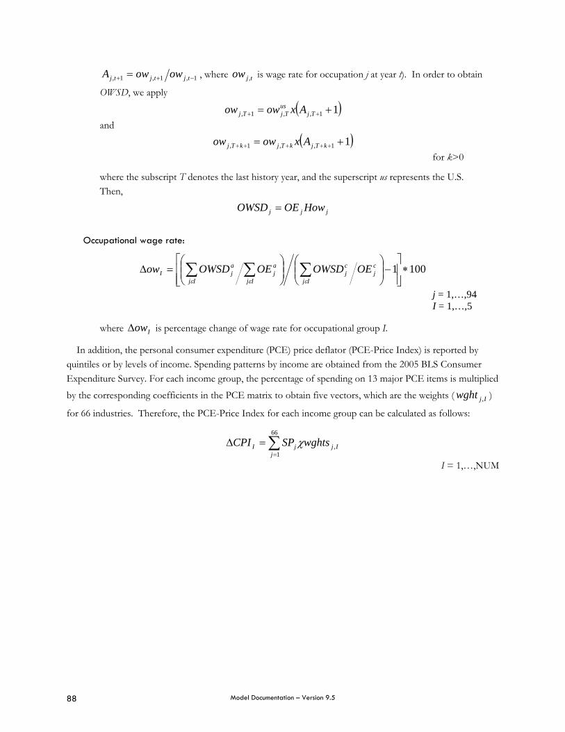
Model Documentation – Version 9.5 88
1,1,1, −++ = tjtjtj owowA , where tjow , is wage rate for occupation j at year t). In order to obtain
OWSD, we apply
( )11,,1, += ++ Tjus
TjTj Axowow and
( )11,,1, += +++++ kTjkTjkTj Axowow for k>0
where the subscript T denotes the last history year, and the superscript us represents the U.S. Then,
jjj HowOEOWSD =
Occupational wage rate:
1001 ∗⎥⎥⎦
⎤
⎢⎢⎣
⎡−⎟⎟
⎠
⎞⎜⎜⎝
⎛⎟⎟⎠
⎞⎜⎜⎝
⎛=Δ ∑∑∑ c
jIj
cj
Ij
aj
Ij
ajI OEOWSDOEOWSDow
εεε
j = 1,…,94 I = 1,…,5
where IowΔ is percentage change of wage rate for occupational group I.
In addition, the personal consumer expenditure (PCE) price deflator (PCE-Price Index) is reported by quintiles or by levels of income. Spending patterns by income are obtained from the 2005 BLS Consumer Expenditure Survey. For each income group, the percentage of spending on 13 major PCE items is multiplied
by the corresponding coefficients in the PCE matrix to obtain five vectors, which are the weights ( Ijwght , )
for 66 industries. Therefore, the PCE-Price Index for each income group can be calculated as follows:
Ijj
jI wghtsSPCPI ,
66
1χ∑
=
=Δ
I = 1,…,NUM

Model Documentation – Version 9.5 89
Chapter 9: The Structural Consumption Equation for REMI Policy Insight Version 9.5 – George Treyz, Frederick Treyz, Nick Mata, Sherri Lawrence, Jerry Hayes
Table of Contents
Introduction.............................................................................................................................. 90
I. Demographic and Regional Influences........................................................................ 91
II. The Consumption Equation ......................................................................................... 94
III. Calibration and Estimation.......................................................................................... 98
IV. Simulations ............................................................................................................... 102
Appendix I. Comparison of Treyz et al (V 9.5) and Treyz and Petraglia (V 9.0) Methodology............................................................................................................... 106
Appendix II. Personal Consumption Expenditure Categories ...................................... 111
Appendix III. Variable Definitions................................................................................ 113
Appendix IV. List of Tables .......................................................................................... 115
Appendix V. References .............................................................................................. 116

Model Documentation – Version 9.5 90
Introduction
Consumers are the king, queen, and court of the U.S. economy. Over 70% of national economic activity depends on the consumer. At the regional level, consumption patterns differ widely by city and state.
For policy analysis, consumption matters for a broad range of issues. Consumption issues are central to
the formulation of policies concerning sales, property, and fuel taxes, and to the provision of environmental and energy efficiency incentives. Economic development is increasingly geared toward the expenditures of local residents, particularly in services such as housing and medical care.
This paper (Treyz et al) describes the new REMI consumption equation, for REMI Policy Insight Version 9.5. This equation replaces the earlier formulation of Treyz and Petraglia (2001) that we used in Versions 9.0 and preceding versions. Treyz et al encompasses all aspects of the earlier equations, and is updated and improved in several important ways. The significant improvement in the new equation is to link each consumption category to changes in population by age group. The 9.5 equation also uses data from more recent and comprehensive data sets and more accurately calibrates to the last history year for each U.S. county. We have also re-estimated income and price elasticities using recent U.S. data series’ and updated consumption categories.
Part I discusses demographic and regional influences, and presents basic consumption data. Part II describes the Version 9.5 model equations, and Part III shows the calibration and estimation results. Part IV shows example policy simulations in REMI Policy Insight, focusing on consumption responses. The Appendix compares the Version 9.5 equation to the Version 9.0 equation, including a comparison of simulation results.
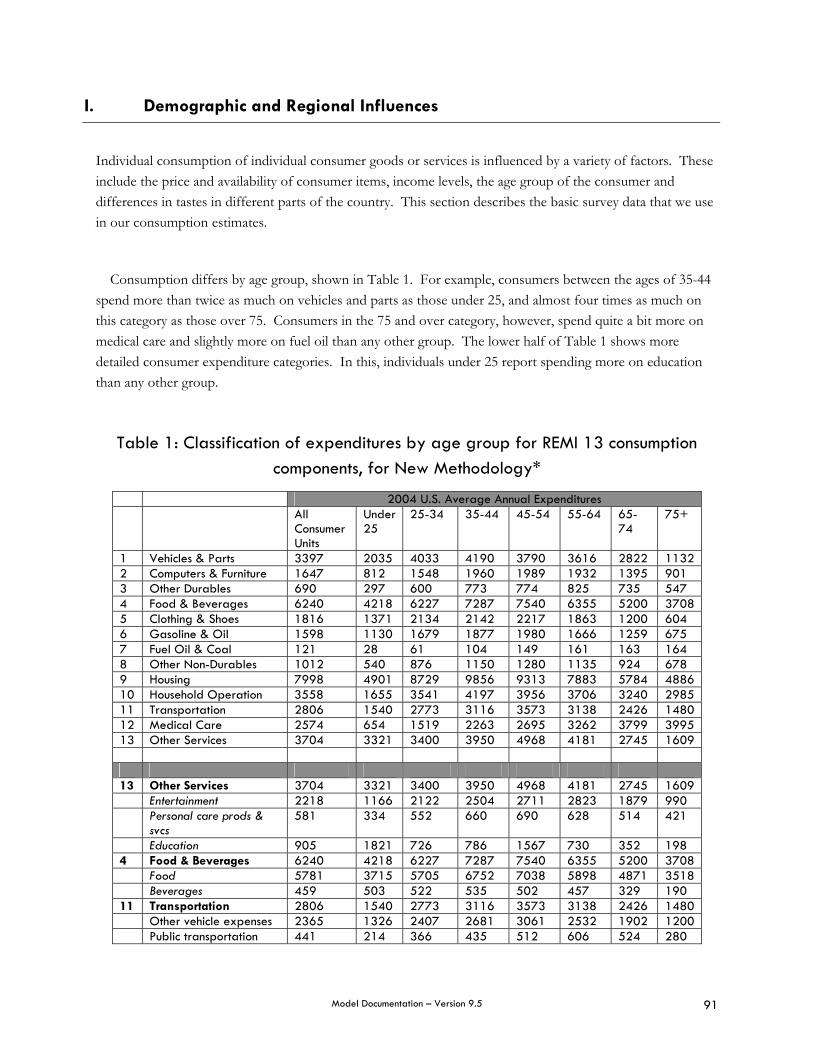
Model Documentation – Version 9.5 91
I. Demographic and Regional Influences
Individual consumption of individual consumer goods or services is influenced by a variety of factors. These include the price and availability of consumer items, income levels, the age group of the consumer and differences in tastes in different parts of the country. This section describes the basic survey data that we use in our consumption estimates.
Consumption differs by age group, shown in Table 1. For example, consumers between the ages of 35-44 spend more than twice as much on vehicles and parts as those under 25, and almost four times as much on this category as those over 75. Consumers in the 75 and over category, however, spend quite a bit more on medical care and slightly more on fuel oil than any other group. The lower half of Table 1 shows more detailed consumer expenditure categories. In this, individuals under 25 report spending more on education than any other group.
Table 1: Classification of expenditures by age group for REMI 13 consumption components, for New Methodology*
2004 U.S. Average Annual Expenditures
All Consumer Units
Under 25
25-34 35-44 45-54 55-64 65-74
75+
1 Vehicles & Parts 3397 2035 4033 4190 3790 3616 2822 1132 2 Computers & Furniture 1647 812 1548 1960 1989 1932 1395 901 3 Other Durables 690 297 600 773 774 825 735 547 4 Food & Beverages 6240 4218 6227 7287 7540 6355 5200 3708 5 Clothing & Shoes 1816 1371 2134 2142 2217 1863 1200 604 6 Gasoline & Oil 1598 1130 1679 1877 1980 1666 1259 675 7 Fuel Oil & Coal 121 28 61 104 149 161 163 164 8 Other Non-Durables 1012 540 876 1150 1280 1135 924 678 9 Housing 7998 4901 8729 9856 9313 7883 5784 4886 10 Household Operation 3558 1655 3541 4197 3956 3706 3240 2985 11 Transportation 2806 1540 2773 3116 3573 3138 2426 1480 12 Medical Care 2574 654 1519 2263 2695 3262 3799 3995 13 Other Services 3704 3321 3400 3950 4968 4181 2745 1609 13 Other Services 3704 3321 3400 3950 4968 4181 2745 1609 Entertainment 2218 1166 2122 2504 2711 2823 1879 990 Personal care prods &
svcs 581 334 552 660 690 628 514 421
Education 905 1821 726 786 1567 730 352 198 4 Food & Beverages 6240 4218 6227 7287 7540 6355 5200 3708 Food 5781 3715 5705 6752 7038 5898 4871 3518 Beverages 459 503 522 535 502 457 329 190 11 Transportation 2806 1540 2773 3116 3573 3138 2426 1480 Other vehicle expenses 2365 1326 2407 2681 3061 2532 1902 1200 Public transportation 441 214 366 435 512 606 524 280
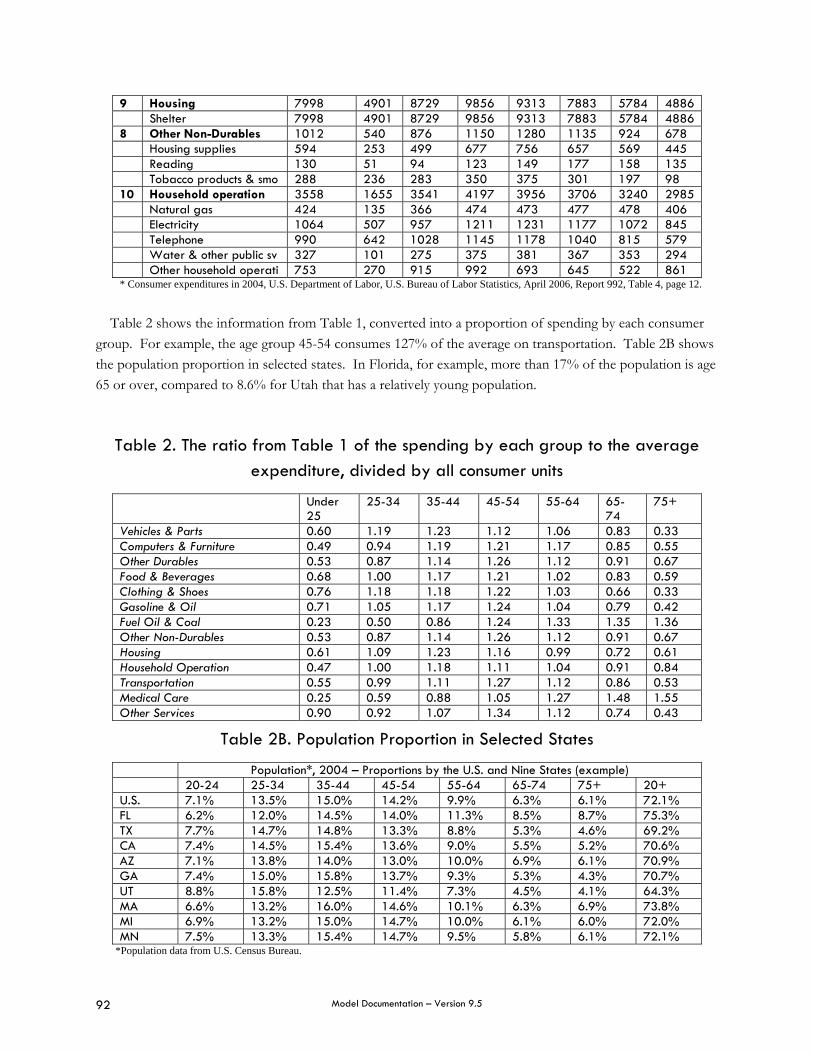
Model Documentation – Version 9.5 92
9 Housing 7998 4901 8729 9856 9313 7883 5784 4886 Shelter 7998 4901 8729 9856 9313 7883 5784 4886 8 Other Non-Durables 1012 540 876 1150 1280 1135 924 678 Housing supplies 594 253 499 677 756 657 569 445 Reading 130 51 94 123 149 177 158 135 Tobacco products & smo 288 236 283 350 375 301 197 98 10 Household operation 3558 1655 3541 4197 3956 3706 3240 2985 Natural gas 424 135 366 474 473 477 478 406 Electricity 1064 507 957 1211 1231 1177 1072 845 Telephone 990 642 1028 1145 1178 1040 815 579 Water & other public sv 327 101 275 375 381 367 353 294 Other household operati 753 270 915 992 693 645 522 861 * Consumer expenditures in 2004, U.S. Department of Labor, U.S. Bureau of Labor Statistics, April 2006, Report 992, Table 4, page 12.
Table 2 shows the information from Table 1, converted into a proportion of spending by each consumer group. For example, the age group 45-54 consumes 127% of the average on transportation. Table 2B shows the population proportion in selected states. In Florida, for example, more than 17% of the population is age 65 or over, compared to 8.6% for Utah that has a relatively young population.
Table 2. The ratio from Table 1 of the spending by each group to the average expenditure, divided by all consumer units
Under 25
25-34 35-44 45-54 55-64 65-74
75+
Vehicles & Parts 0.60 1.19 1.23 1.12 1.06 0.83 0.33 Computers & Furniture 0.49 0.94 1.19 1.21 1.17 0.85 0.55 Other Durables 0.53 0.87 1.14 1.26 1.12 0.91 0.67 Food & Beverages 0.68 1.00 1.17 1.21 1.02 0.83 0.59 Clothing & Shoes 0.76 1.18 1.18 1.22 1.03 0.66 0.33 Gasoline & Oil 0.71 1.05 1.17 1.24 1.04 0.79 0.42 Fuel Oil & Coal 0.23 0.50 0.86 1.24 1.33 1.35 1.36 Other Non-Durables 0.53 0.87 1.14 1.26 1.12 0.91 0.67 Housing 0.61 1.09 1.23 1.16 0.99 0.72 0.61 Household Operation 0.47 1.00 1.18 1.11 1.04 0.91 0.84 Transportation 0.55 0.99 1.11 1.27 1.12 0.86 0.53 Medical Care 0.25 0.59 0.88 1.05 1.27 1.48 1.55 Other Services 0.90 0.92 1.07 1.34 1.12 0.74 0.43
Table 2B. Population Proportion in Selected States
Population*, 2004 – Proportions by the U.S. and Nine States (example) 20-24 25-34 35-44 45-54 55-64 65-74 75+ 20+ U.S. 7.1% 13.5% 15.0% 14.2% 9.9% 6.3% 6.1% 72.1% FL 6.2% 12.0% 14.5% 14.0% 11.3% 8.5% 8.7% 75.3% TX 7.7% 14.7% 14.8% 13.3% 8.8% 5.3% 4.6% 69.2% CA 7.4% 14.5% 15.4% 13.6% 9.0% 5.5% 5.2% 70.6% AZ 7.1% 13.8% 14.0% 13.0% 10.0% 6.9% 6.1% 70.9% GA 7.4% 15.0% 15.8% 13.7% 9.3% 5.3% 4.3% 70.7% UT 8.8% 15.8% 12.5% 11.4% 7.3% 4.5% 4.1% 64.3% MA 6.6% 13.2% 16.0% 14.6% 10.1% 6.3% 6.9% 73.8% MI 6.9% 13.2% 15.0% 14.7% 10.0% 6.1% 6.0% 72.0% MN 7.5% 13.3% 15.4% 14.7% 9.5% 5.8% 6.1% 72.1%
*Population data from U.S. Census Bureau.

Model Documentation – Version 9.5 93
Table 3 shows 2004 survey data on consumption in the four major regions of the U.S. The relative
expenditures for the Northeast, Midwest, South, and West show large differences among these regions for 13 consumption goods and services. For example, families in the Northeast spend 94% of the average U.S. expenditures on Vehicles and Parts, while families in the West spend 117% of the national average in the same category. In the fuel, oil, and coal category, the Northeast spends 266% while the West spends 39.7% of the U.S. average.
Table 3: Average Expenditures as a % of National Expenditures
Northeast Midwest South West Vehicles & Parts 94.1% 97.6% 94.1% 117.1% Computers & Furniture 99.0% 107.8% 86.9% 113.6% Other Durables 110.1% 115.5% 74.2% 117.2% Food & Beverages 112.1% 96.5% 90.8% 108.3% Clothing & Shoes 119.8% 92.1% 90.5% 106.6% Gasoline & Oil 86.7% 101.4% 100.0% 109.8% Fuel Oil & Coal 266.1% 86.8% 57.0% 39.7% Other Non-Durables 101.5% 113.7% 92.7% 96.7% Housing 120.4% 91.8% 82.8% 118.9% Household Operation 100.3% 100.0% 100.6% 98.8% Transportation 108.3% 98.9% 87.0% 115.1% Medical Care 92.1% 111.1% 97.4% 99.5% Other Services 102.6% 99.9% 89.3% 115.4% * Consumer expenditures in 2004, U.S. Department of Labor, U.S. Bureau of Labor Statistics, April 2006, Report 992, Table 11, page 18-19.
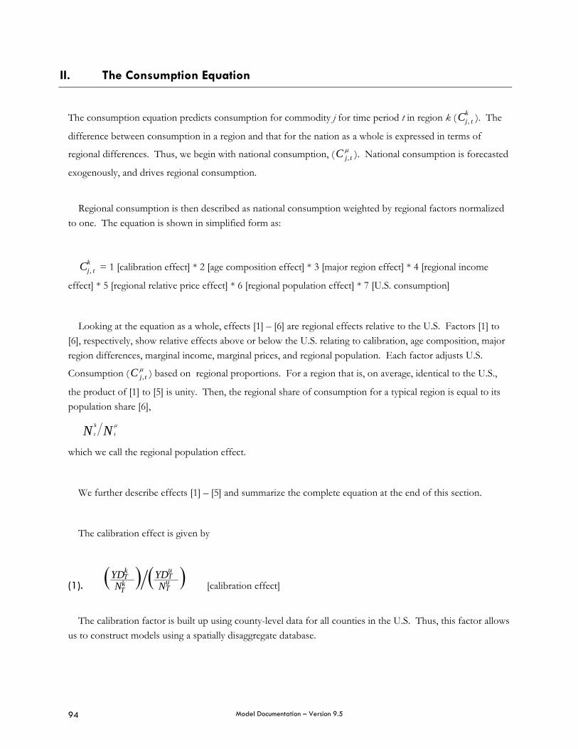
Model Documentation – Version 9.5 94
II. The Consumption Equation
The consumption equation predicts consumption for commodity j for time period t in region k ( tjkC , ). The
difference between consumption in a region and that for the nation as a whole is expressed in terms of
regional differences. Thus, we begin with national consumption, ( μtjC , ). National consumption is forecasted
exogenously, and drives regional consumption.
Regional consumption is then described as national consumption weighted by regional factors normalized
to one. The equation is shown in simplified form as:
tjkC , = 1 [calibration effect] * 2 [age composition effect] * 3 [major region effect] * 4 [regional income
effect] * 5 [regional relative price effect] * 6 [regional population effect] * 7 [U.S. consumption]
Looking at the equation as a whole, effects [1] – [6] are regional effects relative to the U.S. Factors [1] to [6], respectively, show relative effects above or below the U.S. relating to calibration, age composition, major region differences, marginal income, marginal prices, and regional population. Each factor adjusts U.S.
Consumption ( μtjC , ) based on regional proportions. For a region that is, on average, identical to the U.S.,
the product of [1] to [5] is unity. Then, the regional share of consumption for a typical region is equal to its population share [6],
NN t
k
t
μ
which we call the regional population effect.
We further describe effects [1] – [5] and summarize the complete equation at the end of this section.
The calibration effect is given by
(1). ( ) ( )TuTu
TkTk
NYD
NYD
[calibration effect]
The calibration factor is built up using county-level data for all counties in the U.S. Thus, this factor allows
us to construct models using a spatially disaggregate database.

Model Documentation – Version 9.5 95
Also, we added this adjustment to the Treyz and Petraglia equation in the 2002 economic geography version of REMI Policy Insight. The new economic geography method develops key relationships, including trade flows, using county-level data. We calculate these relationships using basic data concepts such as nominal disposable income, and for computational reasons we do not calculate the economic geography database using derived concepts such as real disposable income. Thus, the calibration factor adjusts the
consumption equation to normalize relative regional disposable income ( TkYD ) in the base year T.
We calculate the relative effect of population distribution in personal consumption using the age composition effect. This is effect is shown by,
Where %DG is the percentage of population in each demographic group and ( ujlPC , ) is the U.S.
propensity to consume for each consumption category. The differences in the propensity to consume by age
group ( ujlPC , ) are determined by the average U.S. expenditure by age group (l) on item (j) relative to the
average expenditure of all age groups on item (j) in the U.S. Thus, the U.S. propensity to consume for different commodities by age group is weighted by the local age composition. (See Table 2 above).
Next, we proceed to incorporate the use of survey data that show the average spending for each consumption commodity for the four major parts of the country. The major region effect is shown as
(3). ⎥⎦
⎤⎢⎣
⎡)2(
2004.2004,
EffectCompAge
jujR
CC
[major region effect]
Consumption is adjusted to reflect regional differences for the four major regions of the U.S. ( jRC ). The
major region effect shows the difference in consumption patterns, after adjusting for regional demographic composition. Thus, we divide by the Age Comp Effect (2). This regional effect replaced the fixed effect in the previous consumption equation, estimated by an econometric estimate for each of the limited number of metro area data. These were also used for other areas and states based on these locations. An advantage of adjusting the intercept by (2) is that we use the calculated Age Composition Effect for each county in the base year. Thus we can predict the consumption change in the future due to the population change.
=l
( ) ( )∑∑==
××7
1,
7
1, %%
ljl
ulu
ljl
ulk PCDGPCDG(2). [age composition effect]
Seven age groups based on the age of the reference person

Model Documentation – Version 9.5 96
In the Treyz et al version, we use a survey-based structural approach in contrast to the earlier econometric approach based on limited data from select metropolitan areas.
The regional income (4) and price effects (5) for each local region depend on elasticities that are estimated
econometrically. In order to estimate the income ( jβ ) and price ( jγ ) elasticities, the new equation is based
on a national time series from 1995 to 2006 and derived from U.S. aggregate data. The procedure for making these estimates is reported after Table 8. The regional income effect,
(4).
j
Tu
Tu
Tk T
k
tu
tu
tk
tk
NRYD
NRYD
NRYD
NRYD
β
⎥⎥⎦
⎤
⎢⎢⎣
⎡⎟⎟⎠
⎞⎜⎜⎝
⎛⎟⎟⎠
⎞⎜⎜⎝
⎛ [regional income effect]
shows the change in consumption caused by changes in real disposable income (RYD) per capita. This
concept is divided by the same concept in the nation and normalized to the base year T to show consumption changes relative to the U.S. for the forecast years. The region-specific marginal price effect is given by
(5).
j
TuTj
uTkTj
k
tu
tjutktj
k
PPPP
PPP
Pγ
⎥⎥⎦
⎤
⎢⎢⎣
⎡⎟⎟⎠
⎞⎜⎜⎝
⎛⎟⎟⎠
⎞⎜⎜⎝
⎛,
,
,
,
[regional relative price effect]
Where ( jP ) is the price of commodity (j) and ( jγ ) is the respective price elasticity.
The Regional Population Effect,
(6). ⎟⎟⎠
⎞⎜⎜⎝
⎛
tu
kt
NN
[regional population effect]
drives regional consumption with U.S. consumption per capita. The national consumption effect,
(7). μtjC , [U.S. consumption]

Model Documentation – Version 9.5 97
changes consumption by the population increase of a region, and the endogenous effects of real disposable income per person as well as price changes in the region.
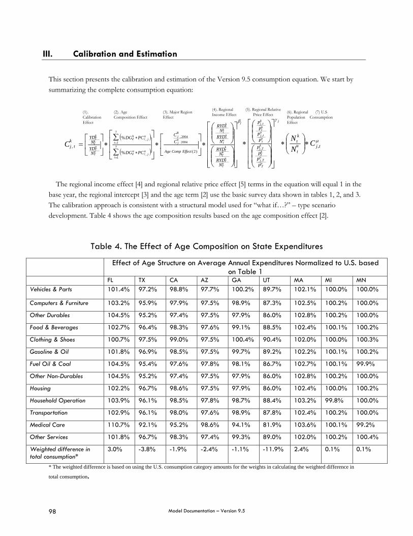
Model Documentation – Version 9.5 98
III. Calibration and Estimation
This section presents the calibration and estimation of the Version 9.5 consumption equation. We start by summarizing the complete consumption equation:
(1). Calibration Effect
(2). Age Composition Effect
(3). Major Region Effect
(4). Regional Income Effect
(5). Regional Relative Price Effect (6). Regional
Population Effect
( )
( )
j
Tu
Tu
Tk T
ktu
tu
tk
tk
jujR
ujt
u
t
ujt
k
TuTu
TkTk
NRYD
NRYD
NRYD
NRYD
CC
PCDG
PCDG
NYDN
YD
tjk
EffectCompAgeC
β
⎥⎥⎥⎥⎥
⎦
⎤
⎢⎢⎢⎢⎢
⎣
⎡
⎟⎟⎠
⎞⎜⎜⎝
⎛
⎟⎟⎠
⎞⎜⎜⎝
⎛
∗⎥⎦
⎤⎢⎣
⎡∗
⎥⎥
⎦
⎤
⎢⎢
⎣
⎡
∑
∑∗⎥
⎦
⎤⎢⎣
⎡=
=
=
∗
∗
)2(
2004.
2004,
7
1,
7
1,
%
%
,
lll
ll μ
γ
tjtu
kt
PPP
PP
PP
P
CNN
j
Tu
TjuTkTj
ktu
tjutktj
k
,
,
,
,
,
∗⎟⎟⎠
⎞⎜⎜⎝
⎛∗
⎥⎥⎥⎥⎥
⎦
⎤
⎢⎢⎢⎢⎢
⎣
⎡
⎟⎟⎠
⎞⎜⎜⎝
⎛
⎟⎟⎠
⎞⎜⎜⎝
⎛
∗
(7) U.S Consumption
The regional income effect [4] and regional relative price effect [5] terms in the equation will equal 1 in the
base year, the regional intercept [3] and the age term [2] use the basic survey data shown in tables 1, 2, and 3. The calibration approach is consistent with a structural model used for “what if…?” – type scenario development. Table 4 shows the age composition results based on the age composition effect [2].
Table 4. The Effect of Age Composition on State Expenditures
Effect of Age Structure on Average Annual Expenditures Normalized to U.S. based on Table 1
FL TX CA AZ GA UT MA MI MN Vehicles & Parts 101.4% 97.2% 98.8% 97.7% 100.2% 89.7% 102.1% 100.0% 100.0%
Computers & Furniture 103.2% 95.9% 97.9% 97.5% 98.9% 87.3% 102.5% 100.2% 100.0%
Other Durables 104.5% 95.2% 97.4% 97.5% 97.9% 86.0% 102.8% 100.2% 100.0%
Food & Beverages 102.7% 96.4% 98.3% 97.6% 99.1% 88.5% 102.4% 100.1% 100.2%
Clothing & Shoes 100.7% 97.5% 99.0% 97.5% 100.4% 90.4% 102.0% 100.0% 100.3%
Gasoline & Oil 101.8% 96.9% 98.5% 97.5% 99.7% 89.2% 102.2% 100.1% 100.2%
Fuel Oil & Coal 104.5% 95.4% 97.6% 97.8% 98.1% 86.7% 102.7% 100.1% 99.9%
Other Non-Durables 104.5% 95.2% 97.4% 97.5% 97.9% 86.0% 102.8% 100.2% 100.0%
Housing 102.2% 96.7% 98.6% 97.5% 97.9% 86.0% 102.4% 100.0% 100.2%
Household Operation 103.9% 96.1% 98.5% 97.8% 98.7% 88.4% 103.2% 99.8% 100.0%
Transportation 102.9% 96.1% 98.0% 97.6% 98.9% 87.8% 102.4% 100.2% 100.0%
Medical Care 110.7% 92.1% 95.2% 98.6% 94.1% 81.9% 103.6% 100.1% 99.2%
Other Services 101.8% 96.7% 98.3% 97.4% 99.3% 89.0% 102.0% 100.2% 100.4%
Weighted difference in total consumption*
3.0% -3.8% -1.9% -2.4% -1.1% -11.9% 2.4% 0.1% 0.1%
* The weighted difference is based on using the U.S. consumption category amounts for the weights in calculating the weighted difference in
total consumption.

Model Documentation – Version 9.5 99
For example, all else being equal, Florida residents would consume 110.7% of the U.S. average for medical
care because it has a larger percent of older people who use more medical care than states with a lower percent of older people. We add up all the state wide demographic effects to show the age structure effects on expenditures for major regions of the U.S. in Table 5.
Table 5: Age Structure Effect on Average Expenditure
Northeast Midwest South West Vehicles & Parts 101.8% 99.8% 100.2% 99.2% Computers & Furniture 102.5% 100.1% 99.9% 98.5% Other Durables 102.8% 100.3% 99.9% 98.2% Food & Beverages 102.3% 100.2% 100.0% 98.7% Clothing & Shoes 101.7% 100.0% 100.1% 99.4% Gasoline & Oil 102.0% 100.1% 100.0% 99.0% Fuel Oil & Coal 104.5% 100.8% 99.6% 96.2% Other Non-Durables 102.8% 100.3% 99.9% 98.2% Housing 102.2% 100.1% 100.0% 98.9% Household Operation 102.8% 100.2% 99.9% 98.3% Transportation 102.4% 100.1% 100.0% 98.6% Medical Care 104.5% 100.8% 99.7% 96.2% Other Services 102.1% 100.3% 100.0% 98.7%
In Table 3 we presented the observed effects by region that are based on survey data.
Table 6 shows the observed area differences (Table 3) divided by the age structure effects (Table 5). The purpose of dividing by Table is because we already have the Table 5 effect as an endogenous factor in the equation.
Table 6: Major region Effect for the Consumption Equation (normalizing for age effects)
Northeast Midwest South West Vehicles & Parts 0.92430 0.97733 0.93889 1.18062 Computers & Furniture 0.96512 1.07646 0.86996 1.15382 Other Durables 1.07194 1.15191 0.74296 1.19405 Food & Beverages 1.09546 0.96294 0.90825 1.09711 Clothing & Shoes 1.17860 0.92105 0.90386 1.07298 Gasoline & Oil 0.85029 1.01307 0.99958 1.10986 Fuel Oil & Coal 2.54773 0.86057 0.57257 0.41222 Other Non-Durables 0.98764 1.13424 0.92804 0.98520 Housing 1.17717 0.91685 0.82818 1.20245 Household Operation 0.97620 0.99823 1.00664 1.00540 Transportation 1.05826 0.98784 0.86982 1.16833 Medical Care 0.88160 1.10258 0.97749 1.03366 Other Services 1.00516 0.99603 0.89301 1.16838
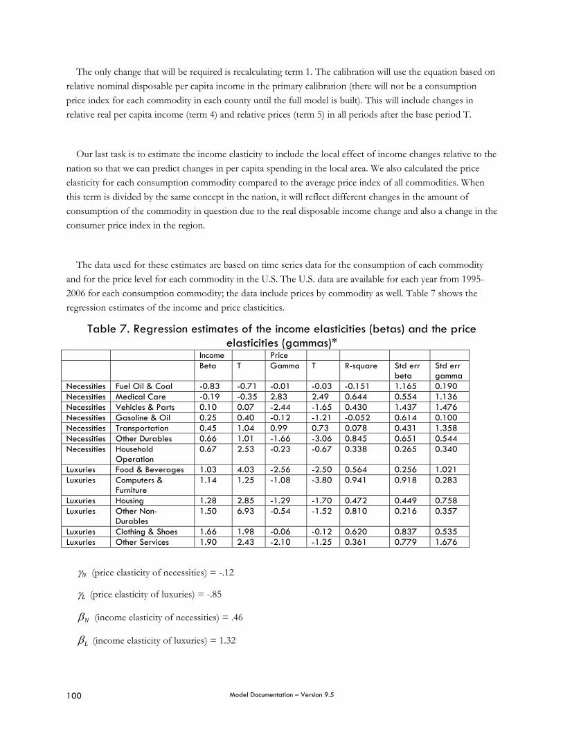
Model Documentation – Version 9.5 100
The only change that will be required is recalculating term 1. The calibration will use the equation based on relative nominal disposable per capita income in the primary calibration (there will not be a consumption price index for each commodity in each county until the full model is built). This will include changes in relative real per capita income (term 4) and relative prices (term 5) in all periods after the base period T.
Our last task is to estimate the income elasticity to include the local effect of income changes relative to the nation so that we can predict changes in per capita spending in the local area. We also calculated the price elasticity for each consumption commodity compared to the average price index of all commodities. When this term is divided by the same concept in the nation, it will reflect different changes in the amount of consumption of the commodity in question due to the real disposable income change and also a change in the consumer price index in the region.
The data used for these estimates are based on time series data for the consumption of each commodity and for the price level for each commodity in the U.S. The U.S. data are available for each year from 1995-2006 for each consumption commodity; the data include prices by commodity as well. Table 7 shows the regression estimates of the income and price elasticities.
Table 7. Regression estimates of the income elasticities (betas) and the price elasticities (gammas)*
Income Price Beta T Gamma T R-square Std err
beta Std err gamma
Necessities Fuel Oil & Coal -0.83 -0.71 -0.01 -0.03 -0.151 1.165 0.190 Necessities Medical Care -0.19 -0.35 2.83 2.49 0.644 0.554 1.136 Necessities Vehicles & Parts 0.10 0.07 -2.44 -1.65 0.430 1.437 1.476 Necessities Gasoline & Oil 0.25 0.40 -0.12 -1.21 -0.052 0.614 0.100 Necessities Transportation 0.45 1.04 0.99 0.73 0.078 0.431 1.358 Necessities Other Durables 0.66 1.01 -1.66 -3.06 0.845 0.651 0.544 Necessities Household
Operation 0.67 2.53 -0.23 -0.67 0.338 0.265 0.340
Luxuries Food & Beverages 1.03 4.03 -2.56 -2.50 0.564 0.256 1.021 Luxuries Computers &
Furniture 1.14 1.25 -1.08 -3.80 0.941 0.918 0.283
Luxuries Housing 1.28 2.85 -1.29 -1.70 0.472 0.449 0.758 Luxuries Other Non-
Durables 1.50 6.93 -0.54 -1.52 0.810 0.216 0.357
Luxuries Clothing & Shoes 1.66 1.98 -0.06 -0.12 0.620 0.837 0.535 Luxuries Other Services 1.90 2.43 -2.10 -1.25 0.361 0.779 1.676
Nγ (price elasticity of necessities) = -.12
Lγ (price elasticity of luxuries) = -.85
Nβ (income elasticity of necessities) = .46
Lβ (income elasticity of luxuries) = 1.32
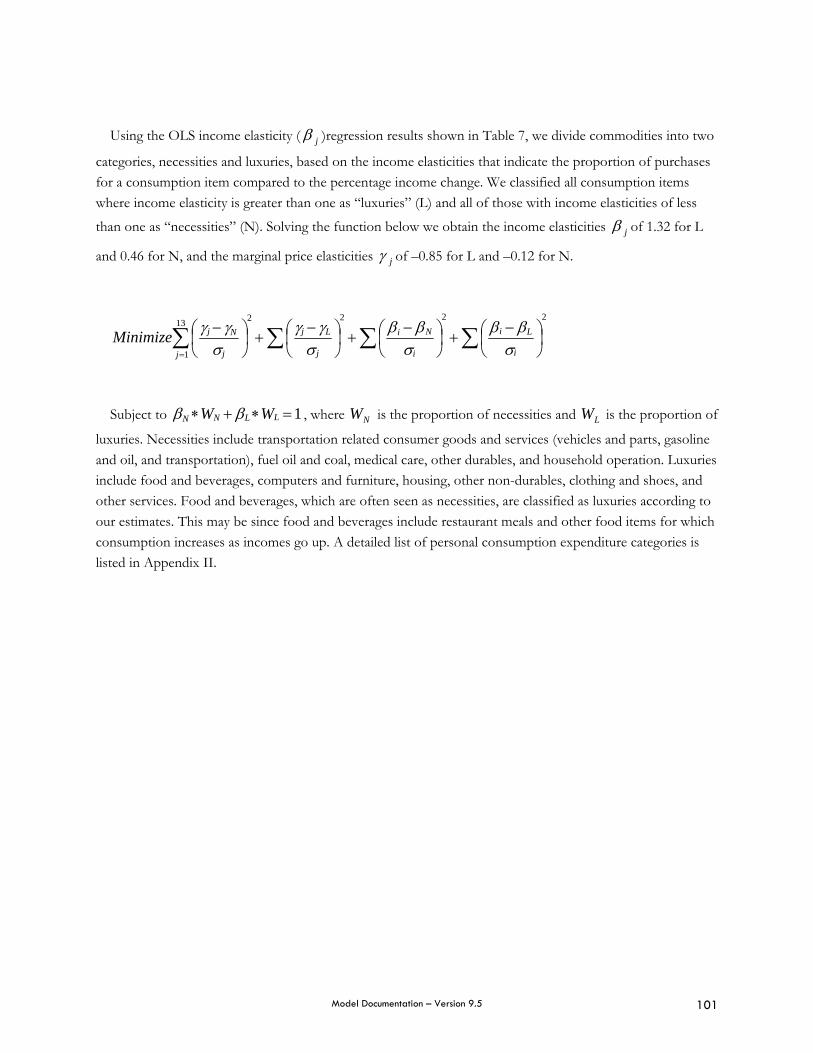
Model Documentation – Version 9.5 101
Using the OLS income elasticity ( jβ )regression results shown in Table 7, we divide commodities into two
categories, necessities and luxuries, based on the income elasticities that indicate the proportion of purchases for a consumption item compared to the percentage income change. We classified all consumption items where income elasticity is greater than one as “luxuries” (L) and all of those with income elasticities of less
than one as “necessities” (N). Solving the function below we obtain the income elasticities jβ of 1.32 for L
and 0.46 for N, and the marginal price elasticities jγ of –0.85 for L and –0.12 for N.
∑ ∑∑ ∑ ⎟⎠⎞
⎜⎝⎛ −
+⎟⎠⎞
⎜⎝⎛ −
+⎟⎠⎞
⎜⎝⎛ −
+⎟⎠⎞
⎜⎝⎛ −
=
22213
1
2
i
Li
i
Ni
j j
Lj
j
NjMinimizeσ
ββσ
ββσ
γγσ
γγ
Subject to 1=∗+∗ LLNN WW ββ , where NW is the proportion of necessities and LW is the proportion of
luxuries. Necessities include transportation related consumer goods and services (vehicles and parts, gasoline and oil, and transportation), fuel oil and coal, medical care, other durables, and household operation. Luxuries include food and beverages, computers and furniture, housing, other non-durables, clothing and shoes, and other services. Food and beverages, which are often seen as necessities, are classified as luxuries according to our estimates. This may be since food and beverages include restaurant meals and other food items for which consumption increases as incomes go up. A detailed list of personal consumption expenditure categories is listed in Appendix II.
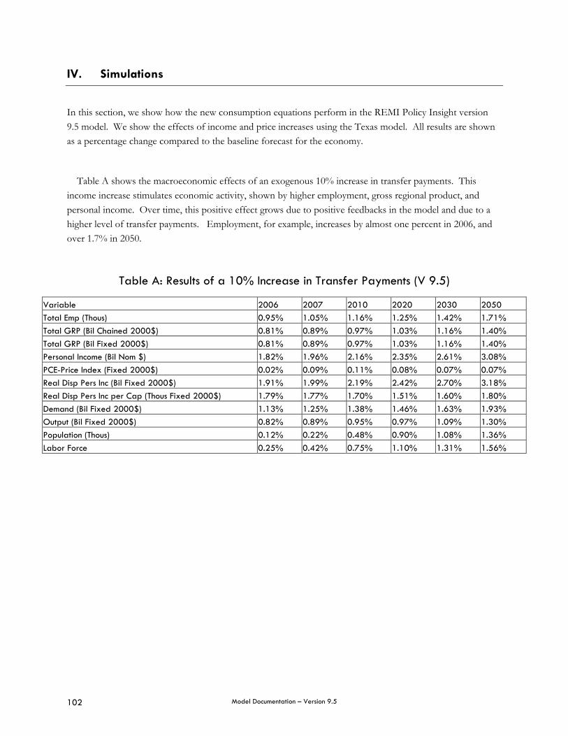
Model Documentation – Version 9.5 102
IV. Simulations
In this section, we show how the new consumption equations perform in the REMI Policy Insight version 9.5 model. We show the effects of income and price increases using the Texas model. All results are shown as a percentage change compared to the baseline forecast for the economy.
Table A shows the macroeconomic effects of an exogenous 10% increase in transfer payments. This income increase stimulates economic activity, shown by higher employment, gross regional product, and personal income. Over time, this positive effect grows due to positive feedbacks in the model and due to a higher level of transfer payments. Employment, for example, increases by almost one percent in 2006, and over 1.7% in 2050.
Table A: Results of a 10% Increase in Transfer Payments (V 9.5)
Variable 2006 2007 2010 2020 2030 2050 Total Emp (Thous) 0.95% 1.05% 1.16% 1.25% 1.42% 1.71% Total GRP (Bil Chained 2000$) 0.81% 0.89% 0.97% 1.03% 1.16% 1.40% Total GRP (Bil Fixed 2000$) 0.81% 0.89% 0.97% 1.03% 1.16% 1.40% Personal Income (Bil Nom $) 1.82% 1.96% 2.16% 2.35% 2.61% 3.08% PCE-Price Index (Fixed 2000$) 0.02% 0.09% 0.11% 0.08% 0.07% 0.07% Real Disp Pers Inc (Bil Fixed 2000$) 1.91% 1.99% 2.19% 2.42% 2.70% 3.18% Real Disp Pers Inc per Cap (Thous Fixed 2000$) 1.79% 1.77% 1.70% 1.51% 1.60% 1.80% Demand (Bil Fixed 2000$) 1.13% 1.25% 1.38% 1.46% 1.63% 1.93% Output (Bil Fixed 2000$) 0.82% 0.89% 0.95% 0.97% 1.09% 1.30% Population (Thous) 0.12% 0.22% 0.48% 0.90% 1.08% 1.36% Labor Force 0.25% 0.42% 0.75% 1.10% 1.31% 1.56%
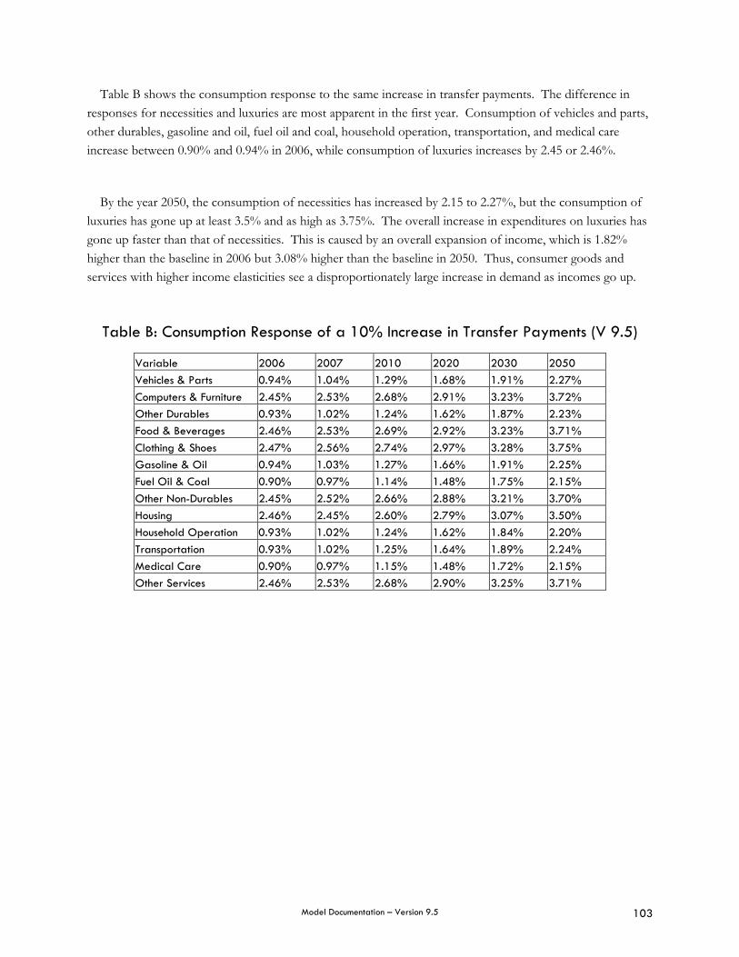
Model Documentation – Version 9.5 103
Table B shows the consumption response to the same increase in transfer payments. The difference in responses for necessities and luxuries are most apparent in the first year. Consumption of vehicles and parts, other durables, gasoline and oil, fuel oil and coal, household operation, transportation, and medical care increase between 0.90% and 0.94% in 2006, while consumption of luxuries increases by 2.45 or 2.46%.
By the year 2050, the consumption of necessities has increased by 2.15 to 2.27%, but the consumption of luxuries has gone up at least 3.5% and as high as 3.75%. The overall increase in expenditures on luxuries has gone up faster than that of necessities. This is caused by an overall expansion of income, which is 1.82% higher than the baseline in 2006 but 3.08% higher than the baseline in 2050. Thus, consumer goods and services with higher income elasticities see a disproportionately large increase in demand as incomes go up.
Table B: Consumption Response of a 10% Increase in Transfer Payments (V 9.5)
Variable 2006 2007 2010 2020 2030 2050 Vehicles & Parts 0.94% 1.04% 1.29% 1.68% 1.91% 2.27% Computers & Furniture 2.45% 2.53% 2.68% 2.91% 3.23% 3.72% Other Durables 0.93% 1.02% 1.24% 1.62% 1.87% 2.23% Food & Beverages 2.46% 2.53% 2.69% 2.92% 3.23% 3.71% Clothing & Shoes 2.47% 2.56% 2.74% 2.97% 3.28% 3.75% Gasoline & Oil 0.94% 1.03% 1.27% 1.66% 1.91% 2.25% Fuel Oil & Coal 0.90% 0.97% 1.14% 1.48% 1.75% 2.15% Other Non-Durables 2.45% 2.52% 2.66% 2.88% 3.21% 3.70% Housing 2.46% 2.45% 2.60% 2.79% 3.07% 3.50% Household Operation 0.93% 1.02% 1.24% 1.62% 1.84% 2.20% Transportation 0.93% 1.02% 1.25% 1.64% 1.89% 2.24% Medical Care 0.90% 0.97% 1.15% 1.48% 1.72% 2.15% Other Services 2.46% 2.53% 2.68% 2.90% 3.25% 3.71%
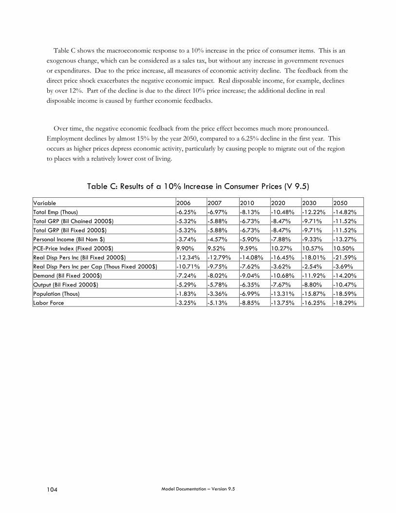
Model Documentation – Version 9.5 104
Table C shows the macroeconomic response to a 10% increase in the price of consumer items. This is an exogenous change, which can be considered as a sales tax, but without any increase in government revenues or expenditures. Due to the price increase, all measures of economic activity decline. The feedback from the direct price shock exacerbates the negative economic impact. Real disposable income, for example, declines by over 12%. Part of the decline is due to the direct 10% price increase; the additional decline in real disposable income is caused by further economic feedbacks.
Over time, the negative economic feedback from the price effect becomes much more pronounced. Employment declines by almost 15% by the year 2050, compared to a 6.25% decline in the first year. This occurs as higher prices depress economic activity, particularly by causing people to migrate out of the region to places with a relatively lower cost of living.
Table C: Results of a 10% Increase in Consumer Prices (V 9.5)
Variable 2006 2007 2010 2020 2030 2050 Total Emp (Thous) -6.25% -6.97% -8.13% -10.48% -12.22% -14.82% Total GRP (Bil Chained 2000$) -5.32% -5.88% -6.73% -8.47% -9.71% -11.52% Total GRP (Bil Fixed 2000$) -5.32% -5.88% -6.73% -8.47% -9.71% -11.52% Personal Income (Bil Nom $) -3.74% -4.57% -5.90% -7.88% -9.33% -13.27% PCE-Price Index (Fixed 2000$) 9.90% 9.52% 9.59% 10.27% 10.57% 10.50% Real Disp Pers Inc (Bil Fixed 2000$) -12.34% -12.79% -14.08% -16.45% -18.01% -21.59% Real Disp Pers Inc per Cap (Thous Fixed 2000$) -10.71% -9.75% -7.62% -3.62% -2.54% -3.69% Demand (Bil Fixed 2000$) -7.24% -8.02% -9.04% -10.68% -11.92% -14.20% Output (Bil Fixed 2000$) -5.29% -5.78% -6.35% -7.67% -8.80% -10.47% Population (Thous) -1.83% -3.36% -6.99% -13.31% -15.87% -18.59% Labor Force -3.25% -5.13% -8.85% -13.75% -16.25% -18.29%

Model Documentation – Version 9.5 105
Table D. details the change in consumption by category in response to the price increase. Consumption of luxuries declines by over 15% in the first year of the simulation, while that of necessities goes down by 6-7%. By the year 2050, the consumption of all goods and services is down dramatically, ranging from a decline of a little over 20% for household operation to a 23.25% reduction in the consumption of clothing and shoes. In the long run, the overall decline in economic activity has a greater impact on consumption than the price increase. By 2050, the population of the region has declined by over 18% compared to the baseline, and real disposable income has gone down by over 21%. However, the decline in real disposable personal income per capita has narrowed over time as the labor supply goes down, requiring employers to pay higher wages. The initial income per capita decline reduces consumption for luxuries at a much higher rate than for necessities. Thus, the drop in the consumption of luxury goods and services in the first year is about 8% larger than that of necessities, while the gap has narrowed to approximately 3% by 2050.
We already discussed factors (1) and (2) above. Factor (3), [major region effect] is based on dividing Table 3, major region effect, by Table 5, which is the age composition effect. The reason for this is that the age effect is now endogenous to the model.
Table D: Consumption Response of a 10% Increase in Consumer Prices (V 9.5)
Variable 2006 2007 2010 2020 2030 2050 Vehicles & Parts -6.83% -7.92% -10.73% -15.99% -18.18% -20.91% Computers & Furniture -15.22% -15.33% -15.97% -18.05% -19.75% -23.11% Other Durables -6.66% -7.59% -10.04% -15.13% -17.69% -20.42% Food & Beverages -15.28% -15.43% -16.15% -18.16% -19.74% -22.96% Clothing & Shoes -15.38% -15.65% -16.57% -18.71% -20.27% -23.25% Gasoline & Oil -6.79% -7.83% -10.52% -15.75% -18.19% -20.68% Fuel Oil & Coal -6.31% -6.94% -8.76% -13.17% -15.97% -19.71% Other Non-Durables -15.18% -15.24% -15.79% -17.74% -19.49% -22.86% Housing -15.31% -14.98% -15.57% -17.27% -18.46% -21.32% Household Operation -6.68% -7.62% -10.16% -15.17% -17.29% -20.17% Transportation -6.71% -7.68% -10.26% -15.39% -17.92% -20.60% Medical Care -6.32% -6.99% -8.85% -13.11% -15.55% -19.66% Other Services -15.30% -15.42% -16.09% -18.05% -20.05% -23.04%
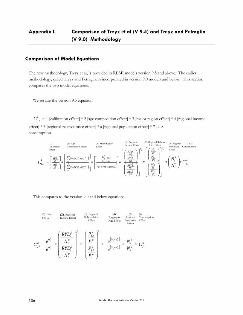
Model Documentation – Version 9.5 106
Appendix I. Comparison of Treyz et al (V 9.5) and Treyz and Petraglia (V 9.0) Methodology
Comparison of Model Equations The new methodology, Treyz et al, is provided in REMI models version 9.5 and above. The earlier methodology, called Treyz and Petraglia, is incorporated in version 9.0 models and below. This section compares the two model equations.
We restate the version 9.5 equation:
tjkC , = 1 [calibration effect] * 2 [age composition effect] * 3 [major region effect] * 4 [regional income
effect] * 5 [regional relative price effect] * 6 [regional population effect] * 7 [U.S. consumption
(1). Calibration Effect
(2). Age Composition Effect
(3). Major Region Effect
(4). Regional Income Effect
(5). Regional Relative Price Effect (6). Regional
Population Effect
( )
( )
j
Tu
Tu
Tk T
ktu
tu
tk
tk
jujR
ujt
u
t
ujt
k
TuTu
TkTk
NRYD
NRYD
NRYD
NRYD
CC
PCDG
PCDG
NYDN
YD
tjk
EffectCompAgeC
β
⎥⎥⎥⎥⎥
⎦
⎤
⎢⎢⎢⎢⎢
⎣
⎡
⎟⎟⎠
⎞⎜⎜⎝
⎛
⎟⎟⎠
⎞⎜⎜⎝
⎛
∗⎥⎦
⎤⎢⎣
⎡∗
⎥⎥
⎦
⎤
⎢⎢
⎣
⎡
∑
∑∗⎥
⎦
⎤⎢⎣
⎡=
=
=
∗
∗
)2(
2004.
2004,
7
1,
7
1,
%
%
,
lll
ll μ
γ
tjtu
kt
PPP
PP
PP
P
CNN
j
Tu
TjuTkTj
ktu
tjutktj
k
,
,
,
,
,
∗⎟⎟⎠
⎞⎜⎜⎝
⎛∗
⎥⎥⎥⎥⎥
⎦
⎤
⎢⎢⎢⎢⎢
⎣
⎡
⎟⎟⎠
⎞⎜⎜⎝
⎛
⎟⎟⎠
⎞⎜⎜⎝
⎛
∗
(7) U.S Consumption
This compares to the version 9.0 and below equation:
ktjC , = u
j
kj
e
eα
α
*
j
ut
ut
kt
kt
NRYD
NRYD
β
⎟⎟⎟⎟⎟
⎠
⎞
⎜⎜⎜⎜⎜
⎝
⎛
*
j
ut
utj
kt
ktj
PPPP
γ
⎟⎟⎟⎟⎟
⎠
⎞
⎜⎜⎜⎜⎜
⎝
⎛
,
,
* ( )
( )utj
ktj
z
z
e
e∗Ψ
∗Ψ
* ut
kt
NN
* utjC ,
(1). Fixed Effect
(2). Regional Income Effect
(3). Regional RelativePrice
Effect
(4). Aggregate Age Effect
(5). Regional
Population Effect
(6) Consumption Effect
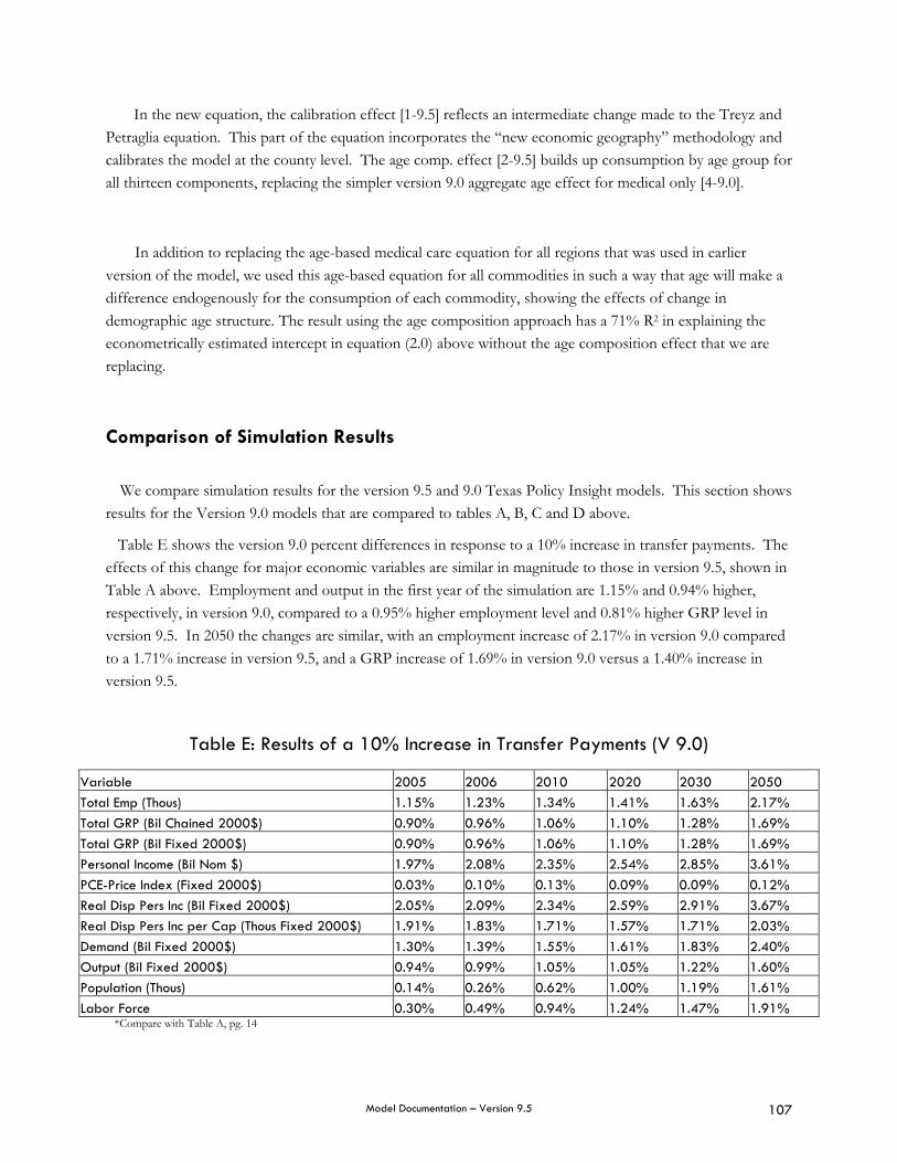
Model Documentation – Version 9.5 107
In the new equation, the calibration effect [1-9.5] reflects an intermediate change made to the Treyz and Petraglia equation. This part of the equation incorporates the “new economic geography” methodology and calibrates the model at the county level. The age comp. effect [2-9.5] builds up consumption by age group for all thirteen components, replacing the simpler version 9.0 aggregate age effect for medical only [4-9.0].
In addition to replacing the age-based medical care equation for all regions that was used in earlier version of the model, we used this age-based equation for all commodities in such a way that age will make a difference endogenously for the consumption of each commodity, showing the effects of change in demographic age structure. The result using the age composition approach has a 71% R2 in explaining the econometrically estimated intercept in equation (2.0) above without the age composition effect that we are replacing.
Comparison of Simulation Results
We compare simulation results for the version 9.5 and 9.0 Texas Policy Insight models. This section shows results for the Version 9.0 models that are compared to tables A, B, C and D above.
Table E shows the version 9.0 percent differences in response to a 10% increase in transfer payments. The effects of this change for major economic variables are similar in magnitude to those in version 9.5, shown in Table A above. Employment and output in the first year of the simulation are 1.15% and 0.94% higher, respectively, in version 9.0, compared to a 0.95% higher employment level and 0.81% higher GRP level in version 9.5. In 2050 the changes are similar, with an employment increase of 2.17% in version 9.0 compared to a 1.71% increase in version 9.5, and a GRP increase of 1.69% in version 9.0 versus a 1.40% increase in version 9.5.
Table E: Results of a 10% Increase in Transfer Payments (V 9.0)
Variable 2005 2006 2010 2020 2030 2050 Total Emp (Thous) 1.15% 1.23% 1.34% 1.41% 1.63% 2.17% Total GRP (Bil Chained 2000$) 0.90% 0.96% 1.06% 1.10% 1.28% 1.69% Total GRP (Bil Fixed 2000$) 0.90% 0.96% 1.06% 1.10% 1.28% 1.69% Personal Income (Bil Nom $) 1.97% 2.08% 2.35% 2.54% 2.85% 3.61% PCE-Price Index (Fixed 2000$) 0.03% 0.10% 0.13% 0.09% 0.09% 0.12% Real Disp Pers Inc (Bil Fixed 2000$) 2.05% 2.09% 2.34% 2.59% 2.91% 3.67% Real Disp Pers Inc per Cap (Thous Fixed 2000$) 1.91% 1.83% 1.71% 1.57% 1.71% 2.03% Demand (Bil Fixed 2000$) 1.30% 1.39% 1.55% 1.61% 1.83% 2.40% Output (Bil Fixed 2000$) 0.94% 0.99% 1.05% 1.05% 1.22% 1.60% Population (Thous) 0.14% 0.26% 0.62% 1.00% 1.19% 1.61% Labor Force 0.30% 0.49% 0.94% 1.24% 1.47% 1.91%
*Compare with Table A, pg. 14
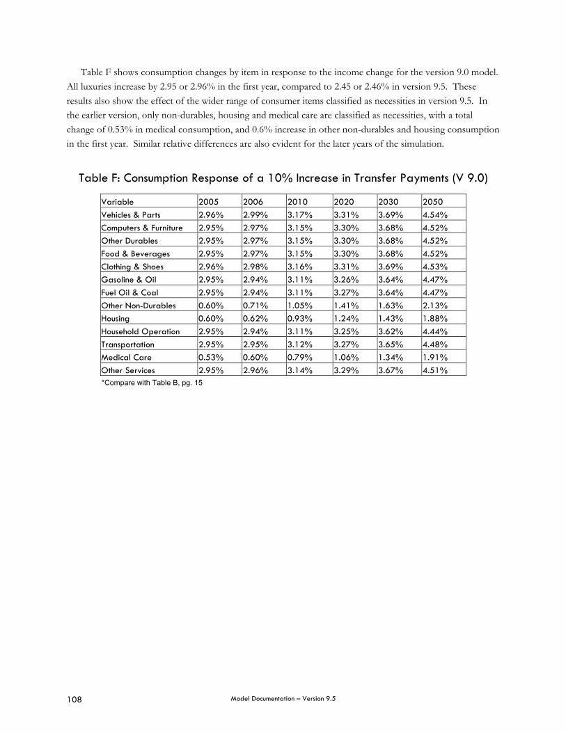
Model Documentation – Version 9.5 108
Table F shows consumption changes by item in response to the income change for the version 9.0 model. All luxuries increase by 2.95 or 2.96% in the first year, compared to 2.45 or 2.46% in version 9.5. These results also show the effect of the wider range of consumer items classified as necessities in version 9.5. In the earlier version, only non-durables, housing and medical care are classified as necessities, with a total change of 0.53% in medical consumption, and 0.6% increase in other non-durables and housing consumption in the first year. Similar relative differences are also evident for the later years of the simulation.
Table F: Consumption Response of a 10% Increase in Transfer Payments (V 9.0)
Variable 2005 2006 2010 2020 2030 2050 Vehicles & Parts 2.96% 2.99% 3.17% 3.31% 3.69% 4.54% Computers & Furniture 2.95% 2.97% 3.15% 3.30% 3.68% 4.52% Other Durables 2.95% 2.97% 3.15% 3.30% 3.68% 4.52% Food & Beverages 2.95% 2.97% 3.15% 3.30% 3.68% 4.52% Clothing & Shoes 2.96% 2.98% 3.16% 3.31% 3.69% 4.53% Gasoline & Oil 2.95% 2.94% 3.11% 3.26% 3.64% 4.47% Fuel Oil & Coal 2.95% 2.94% 3.11% 3.27% 3.64% 4.47% Other Non-Durables 0.60% 0.71% 1.05% 1.41% 1.63% 2.13% Housing 0.60% 0.62% 0.93% 1.24% 1.43% 1.88% Household Operation 2.95% 2.94% 3.11% 3.25% 3.62% 4.44% Transportation 2.95% 2.95% 3.12% 3.27% 3.65% 4.48% Medical Care 0.53% 0.60% 0.79% 1.06% 1.34% 1.91% Other Services 2.95% 2.96% 3.14% 3.29% 3.67% 4.51%
*Compare with Table B, pg. 15
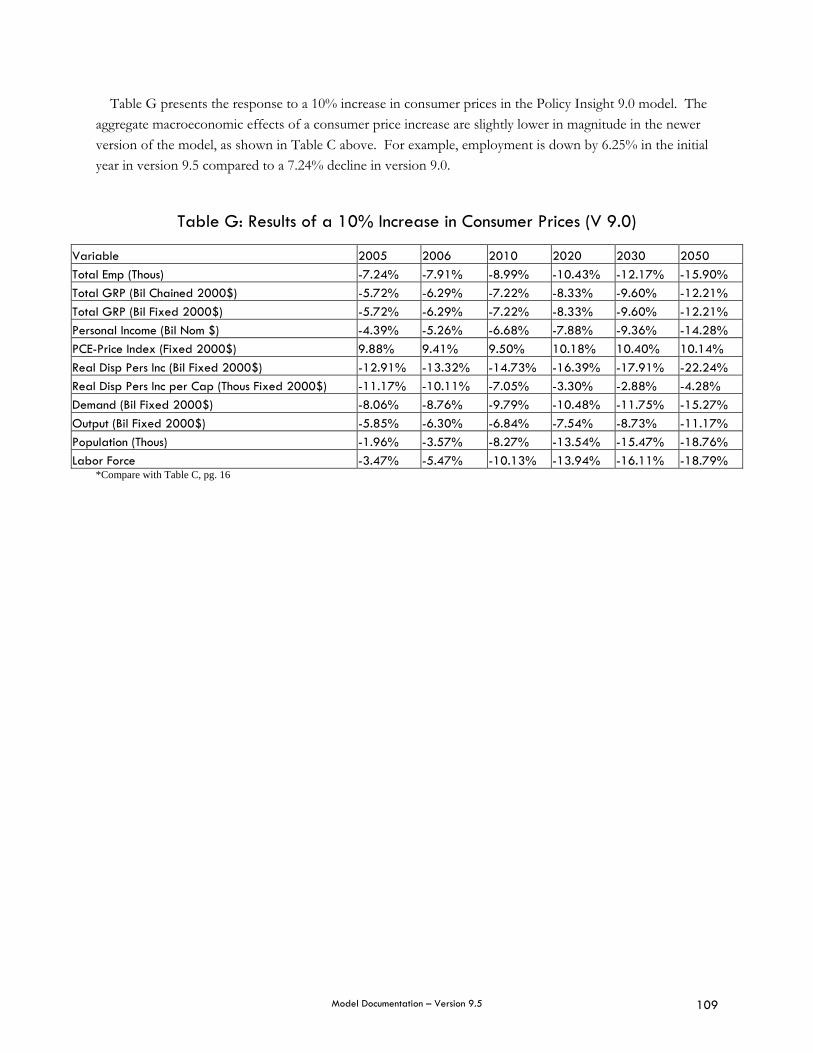
Model Documentation – Version 9.5 109
Table G presents the response to a 10% increase in consumer prices in the Policy Insight 9.0 model. The aggregate macroeconomic effects of a consumer price increase are slightly lower in magnitude in the newer version of the model, as shown in Table C above. For example, employment is down by 6.25% in the initial year in version 9.5 compared to a 7.24% decline in version 9.0.
Table G: Results of a 10% Increase in Consumer Prices (V 9.0)
Variable 2005 2006 2010 2020 2030 2050 Total Emp (Thous) -7.24% -7.91% -8.99% -10.43% -12.17% -15.90% Total GRP (Bil Chained 2000$) -5.72% -6.29% -7.22% -8.33% -9.60% -12.21% Total GRP (Bil Fixed 2000$) -5.72% -6.29% -7.22% -8.33% -9.60% -12.21% Personal Income (Bil Nom $) -4.39% -5.26% -6.68% -7.88% -9.36% -14.28% PCE-Price Index (Fixed 2000$) 9.88% 9.41% 9.50% 10.18% 10.40% 10.14% Real Disp Pers Inc (Bil Fixed 2000$) -12.91% -13.32% -14.73% -16.39% -17.91% -22.24% Real Disp Pers Inc per Cap (Thous Fixed 2000$) -11.17% -10.11% -7.05% -3.30% -2.88% -4.28% Demand (Bil Fixed 2000$) -8.06% -8.76% -9.79% -10.48% -11.75% -15.27% Output (Bil Fixed 2000$) -5.85% -6.30% -6.84% -7.54% -8.73% -11.17% Population (Thous) -1.96% -3.57% -8.27% -13.54% -15.47% -18.76% Labor Force -3.47% -5.47% -10.13% -13.94% -16.11% -18.79%
*Compare with Table C, pg. 16
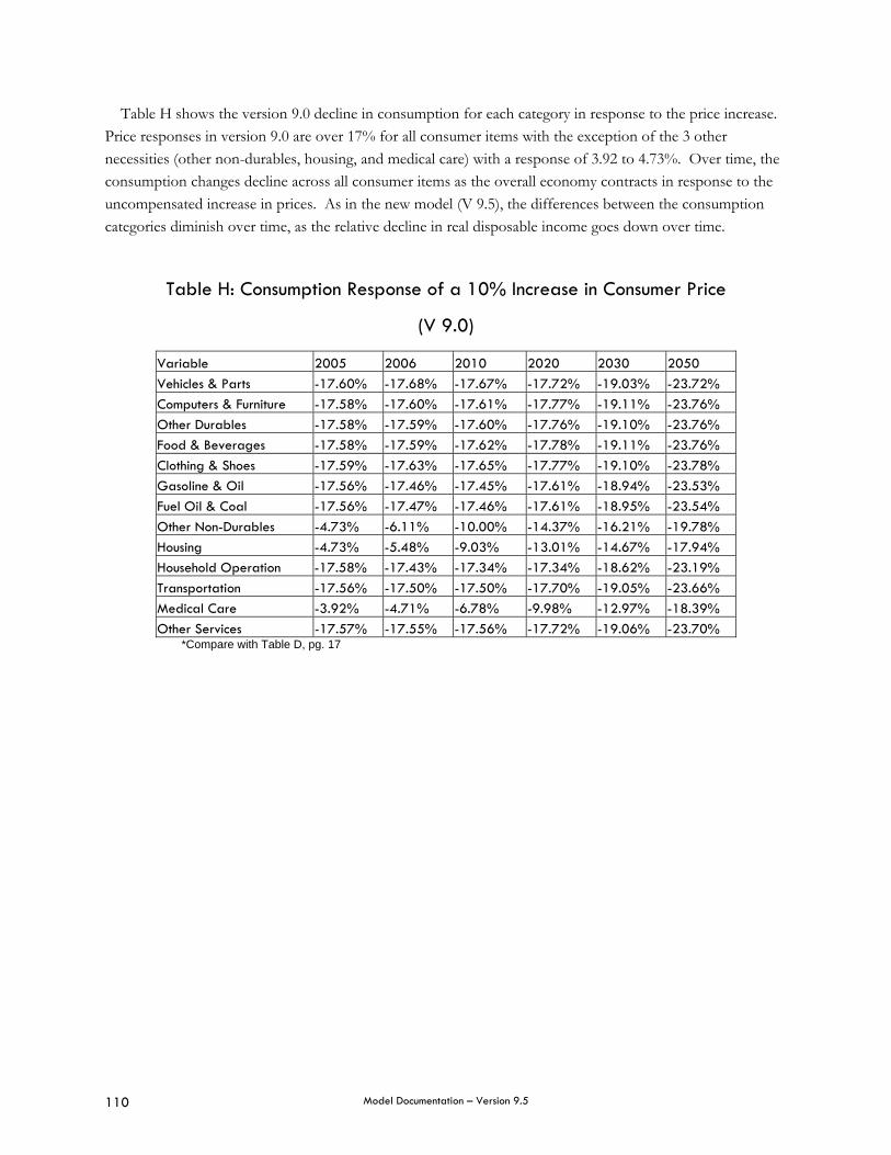
Model Documentation – Version 9.5 110
Table H shows the version 9.0 decline in consumption for each category in response to the price increase. Price responses in version 9.0 are over 17% for all consumer items with the exception of the 3 other necessities (other non-durables, housing, and medical care) with a response of 3.92 to 4.73%. Over time, the consumption changes decline across all consumer items as the overall economy contracts in response to the uncompensated increase in prices. As in the new model (V 9.5), the differences between the consumption categories diminish over time, as the relative decline in real disposable income goes down over time.
Table H: Consumption Response of a 10% Increase in Consumer Price
(V 9.0)
Variable 2005 2006 2010 2020 2030 2050 Vehicles & Parts -17.60% -17.68% -17.67% -17.72% -19.03% -23.72% Computers & Furniture -17.58% -17.60% -17.61% -17.77% -19.11% -23.76% Other Durables -17.58% -17.59% -17.60% -17.76% -19.10% -23.76% Food & Beverages -17.58% -17.59% -17.62% -17.78% -19.11% -23.76% Clothing & Shoes -17.59% -17.63% -17.65% -17.77% -19.10% -23.78% Gasoline & Oil -17.56% -17.46% -17.45% -17.61% -18.94% -23.53% Fuel Oil & Coal -17.56% -17.47% -17.46% -17.61% -18.95% -23.54% Other Non-Durables -4.73% -6.11% -10.00% -14.37% -16.21% -19.78% Housing -4.73% -5.48% -9.03% -13.01% -14.67% -17.94% Household Operation -17.58% -17.43% -17.34% -17.34% -18.62% -23.19% Transportation -17.56% -17.50% -17.50% -17.70% -19.05% -23.66% Medical Care -3.92% -4.71% -6.78% -9.98% -12.97% -18.39% Other Services -17.57% -17.55% -17.56% -17.72% -19.06% -23.70% *Compare with Table D, pg. 17

Model Documentation – Version 9.5 111
Appendix II. Personal Consumption Expenditure Categories
Vehicles & Parts 1 New Autos 2 Used autos 3 Other motor vehicles 4 Tires, tubes, and parts Computers & Furniture 5 Household furniture 6 Household appliances 7 China, glassware, and utensils 8 Video and audio products, and musical instruments 9 Computers, peripherals, and software 10 Other durable house furnishings Other Durables 11 Jewelry and watches 12 Ophthalmic and orthopedic products 13 Books and maps 14 Wheel goods, sporting and photo equipment, boats, and pleasure aircraft Food & Beverages 15 Food for off-premise consumption 16 Purchased meals and beverages 17 Food furnished to employees 18 Food produced and consumed on farms Clothing & Shoes 19 Shoes 20 Women's and children's clothing and accessories, except shoes 21 Men's clothing and accessories, except shoes 22 Military issue clothing Gasoline & Oil 23 Gasoline and oil Other Fuels 24 Other fuels Other Non-Durables 25 Tobacco products 26 Toilet articles and preparations 27 Semi-durable house furnishings 28 Cleaning and miscellaneous household supplies and paper products 29 Stationery and writing supplies 30 Drug preparations and sundries 31 Magazines, newspapers, and sheet music 32 Non-durable toys and sporting goods 33 Flowers, seeds, and potted plants 34 Expenditures abroad by U.S. residents 35 Personal remittances to nonresidents Housing 36 Space rent from owner-occupied non-farm dwellings 37 Rent from tenant-occupied non-farm dwellings 38 Rental value of farm dwellings 39 Other housing (hotels and other lodging places) Household Operation 40 Electricity 41 Gas 42 Telephone and telegraph 43 Water and sanitary services

Model Documentation – Version 9.5 112
44 Domestic services 45 Other household operation Transportation 46 Automobile repair 47 Bridge, tunnel, ferry and road tolls 48 Automobile insurance less claims paid 49 Intracity mass transit 50 Taxicabs 51 Railway transportation 52 Intercity bus 53 Airline transportation 54 Other intercity transportation Medical Care 55 Physicians 56 Dentists 57 Other professional medical services 58 Nonprofit hospitals 59 Proprietary hospitals 60 Government hospitals 61 Nursing homes Other Services 62 Cleaning, storage, and repair of clothing and shoes 63 Miscellaneous personal, clothing, and jewelry services 64 Barbershops, beauty parlors, and health clubs Medical Care 65 Health insurance Other Services 66 Income loss insurance 67 Workman's compensation insurance 68 Brokerage charges and investment counseling 69 Bank service charges 70 Services furnished without payment by financial intermediaries 71 Expense of handling life insurance and pensions 72 Legal services 73 Funeral and burial expenses 74 Other personal business services 75 Radio and television repair 76 Motion picture admissions 77 Legitimate theater admissions 78 Admissions to spectator sports 79 Clubs and fraternal organizations 80 Commercial participant amusements 81 Pari-mutuel net receipts 82 Other recreation services 83 Higher education 84 Nursery, elementary & secondary education 85 Other private education and research 86 Religious and welfare activities 87 Foreign travel by U.S. residents 88 Expenditures in the U.S. by foreigners
Model Documentation – Version 9.5 113
Appendix III. Variable Definitions
Variables
RYD = Real Disposable Income
YD = Nominal Disposable Income
N = Population
P = Price = CIFP
kP = Average price in area for the weighted average of all the commodities that make up total consumption
C = Consumption
%DG = percentage of Demographic Age Group
PC = Propensity to Consume
Subscripts
t = time period
T = last history year time period
j = consumption commodity
Superscripts
k = local region
u = entire nation
jβ = marginal income elasticities: 1.32 for “luxuries” (L), .46 for “necessities” (N)
jγ = marginal price elasticities: -.85 for “luxuries” (L), -.12 for “necessities” (N)
R = major region of the country (Northeast, Midwest, South, West)
The new equation encompasses the aspects of the current consumption equation from a REMI article9 that was published in 2001. In addition to estimating new parameters, we have added an age composition effect on consumption for each of the 13 consumption commodities, based on the age propensity to consume by the age of the reference person. Table 1 shows the basic data for calculating the ratios on the top half of Table 2. For example, the average expenditures as reported by the interviewees under 25 were .60 of the average spent by all consumers on Vehicles and Parts. These national consumption propensities are weighted
9 Consumption Equations for a Multiregional Forecasting and Policy Analysis Model; G.I. Treyz and L.M. Petraglia; Regional Science Perspectives in
Economic Analysis, Elsevier Science B.V. 287-300; 2001.
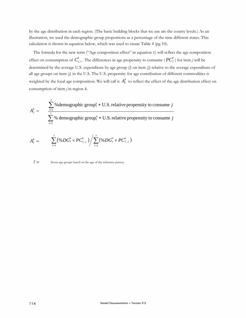
Model Documentation – Version 9.5 114
by the age distribution in each region. (The basic building blocks that we use are the county levels.) As an illustration, we used the demographic group proportions as a percentage of the nine different states. This calculation is shown in equation below, which was used to create Table 4 (pg 10).
The formula for the new term (“Age composition effect” in equation 1) will reflect the age composition
effect on consumption of tjkC , . The differences in age propensity to consume ( j
uPC ) for item j will be
determined by the average U.S. expenditure by age group (l) on item (j) relative to the average expenditure of all age groups on item (j) in the U.S. The U.S. propensity for age contribution of different commodities is
weighted by the local age composition. We will call it jkA to reflect the effect of the age distribution effect on
consumption of item j in region k.
=jkA
( ) ( )∑∑==
××7
1,
7
1, %%
ljl
ulu
ljl
ulk PCDGPCDG
j
j
llu
llk
consume topropensity relative U.S.group cdemographi %
consume topropensity relative U.S.group ic%demograph
7
1
7
1
∗
∗
∑
∑
=
=
=l Seven age groups based on the age of the reference person.
=jkA
Model Documentation – Version 9.5 115
Appendix IV. List of Tables
Table 1. Classification of expenditures by age group for REMI 13 consumption components, for
New Methodology (Page 4) Table 2. The ratio from Table 1 of spending by each group to the average expenditure, divided by all
consumer units. (Page 5) Table 2b. Population Proportion in Selected States (Page 6) Table 3. Average Expenditures as a % of National Expenditures (Page 6) Table 4. The Effect of Age Composition on State Expenditures (Page 10) Table 5. Age Structure Effect on Average Expenditure (Page 11) Table 6. Major region Effect for the Consumption Equation (normalizing for age effects) (Page 12) Table 7. Regression Estimates of the Income Elasticities (betas) and the Price Elasticities (gammas)
(Page 1#) Table A. Results of a 10% Increase in Transfer Payments (Version 9.5) (Page 14) Table B. Total GRP as a Result of a 10% Increase in Transfer Payments (Version 9.5) (Page 15) Table C. Results of a 10% Increase in Consumer Prices (Version 9.5) (Page 16) Table D. Total GRP as a Result of a 10% Increase in Consumer Prices (Version 9.5) (Page 17) Table E. Results of a 10% Increase in Transfer Payments (Version 9.0) (Page 19) Table F. Total GRP as a Result of a 10% Increase in Transfer Payments (Version 9.0) (Page 20) Table G. Results of a 10% Increase in Consumer Prices (Version 9.0) (Page 21) Table H. Total GRP as a Result of a 10% Increase in Consumer Prices (Version 9.0) (Page 22)

Model Documentation – Version 9.5 116
Appendix V. References
Consumer Expenditures in 2004, U.S. Department of Labor, U.S. Bureau of Labor and Statistics, April 2006.
G.I. Treyz and L.M. Petraglia. Consumption Equations for a Multiregional Forecasting and Policy Analysis Model. Regional Science Perspectives in Economic Analysis, Elsevier Science B.V. 287-300; 2001.
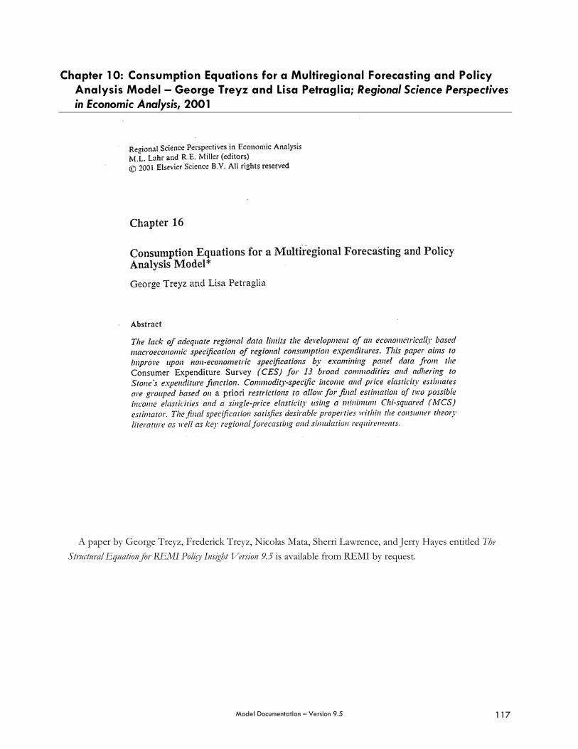
Model Documentation – Version 9.5 117
Chapter 10: Consumption Equations for a Multiregional Forecasting and Policy Analysis Model – George Treyz and Lisa Petraglia; Regional Science Perspectives in Economic Analysis, 2001
A paper by George Treyz, Frederick Treyz, Nicolas Mata, Sherri Lawrence, and Jerry Hayes entitled The Structural Equation for REMI Policy Insight Version 9.5 is available from REMI by request.
Model Documentation – Version 9.5 118
Chapter 11: Economic Implications of Congestion – Glen Weisbrod, Donald Vary, and George Treyz; NCHRP, Report 436, 2001

Model Documentation – Version 9.5 119
Chapter 12: An Evolutionary New Economic Geography Model – Wei Fan, Frederick Treyz, and George Treyz; Journal of Regional Science, 2000
Model Documentation – Version 9.5 120
Chapter 13: Monopolistic Competition Estimates of Interregional Trade Flows in Services – Frederick Treyz and Jim Bumgardner; Regional Cohesion and Competition in the Age of Globalization, 2000
Model Documentation – Version 9.5 121
Chapter 14: The REMI Multiregional U.S. Policy Analysis Model – Frederick Treyz and George Treyz
Model Documentation – Version 9.5 122
Chapter 15: Policy Analysis Applications of REMI Economic Forecasting and Simulation Models – George Treyz; International Journal of Public Administration, 1995

Model Documentation – Version 9.5 123
Chapter 16: Forecasting the Effects of Electric Utility Deregulation: A Hypothetical Scenario for New Jersey – Frederick Treyz and Lisa Petraglia; The Journal of Business Forecasting, 1997

Model Documentation – Version 9.5 124
Chapter 17: Regional Economic Modeling: A Systematic Approach to Economic Forecasting and Policy Analysis – George I. Treyz; 1993
Model Documentation – Version 9.5 125
Chapter 18: Multiregional Stock Adjustment Equations of Residential and Nonresidential Investment in Structures – Dan S. Rickman, G. Shao, and George I. Treyz; Journal of Regional Science, 1993
Model Documentation – Version 9.5 126
Chapter 19: Alternative Labor Market Closures in a Regional Model – Dan S. Rickman and George I. Treyz; Growth and Change, 1993
Model Documentation – Version 9.5 127
Chapter 20: The Dynamics of U.S. Internal Migration – George I. Treyz, et al; The Review of Economics and Statistics, 1993

Model Documentation – Version 9.5 128
Chapter 21: Building U.S. National and Regional Forecasting and Simulation Models – Gang Shao and George I. Treyz; Economics Systems Research, 1993
Model Documentation – Version 9.5 129
Chapter 22: The REMI Economic-Demographic Forecasting and Simulation Model – G.I. Treyz, D.S. Rickman, G. Shao; International Regional Science Review, 1992
Model Documentation – Version 9.5 130
Chapter 23: Migration, Regional Equilibrium, and the Estimation of Compensating Differentials – Michael J. Greenwood, et al; American Economic Review, 1991

Model Documentation – Version 9.5 131
Chapter 24: List of Published Papers and Articles in REMI Files - By Topic with File Numbers
Economic Development 1. Applications of the Wisconsin REMI Model; Wisconsin Department of Development; Randy Pilo; Division
of Research and Planning; (608) 266-8524; 5 pages; September 1988.
2. Poverty in Maine, 1970-1980; Maine State Planning Office Division of Community Services; 29 pages; March 1985.
3. Economic and Fiscal Effects of the Toyota Auto Facility on the Kentucky Economy; Kentucky Legislative Research Commission; 13 pages; October 1986.
4. A Mid-Level Methodology for Evaluating Economic Development Projects; Joseph Persky, W. Wiewel, and D. Felsenstein; 24 pages; 1996.
5. The Economic Effects of the Fort Drum Expansion on the Future of the North County Economy, Phase II Report: Fort Drum Impacts and Phase III/IV Report: Regional Development Opportunities and Alternative Development Scenarios; prepared for the Development Authority of the North County and New York State Urban Development Corporation; Glen Weisbrod; pages 23-69 and pages 93-108, respectively; both April, 1988.
6. An Economic Simulation of Reduced Activity at the Nevada Test Site; Thomas Carroll; University of Nevada; (702) 739-3191; 9 pages with appendices of 27 pages; August 11, 1988.
7. The Economic Impact of the Kansas City Chiefs & Kansas City Royals on the State of Missouri; Frank Lenk, Mid-America Regional Council; (816) 474-4240; 34 pages; February, 1989.
8. A Measure of the Competitiveness of Florida Business Activity: A REMI Model Perspective; Kenneth Trager, The Florida Legislature Office of Economic and Demographic Research; 231 pages; March, 1999.
9. (reserved)
10. (reserved)
11. (reserved)
12. The Economic Impact of Expanding Bartle Hall and Building an 800-Room Hotel; Franklin Lenk; 26 pages; February 6, 1990.
13. The Economic and Fiscal Impacts of a Proposed Development Moratorium in Sarasota County, Florida; Cambridge Systematics, Inc.; 58 pages; May 30, 1990.
14. Report - The Economic and Fiscal Impacts of a Proposed Development Moratorium on Sarasota County, Florida; Cambridge Systematics, Inc.; 167 pages; August 10, 1990.
15. Keeping Jobs for Chicago’s Future; Goose Island Task Force, et al; 39 pages; July, 1990.
16. The Economic Impact of the Horse Racing and Breeding Industry on the State of Minnesota; Minnesota Racing Commission; 9 pages; April, 1991.
Model Documentation – Version 9.5 132
17. Alternative Employment Impacts of the Proposed McCormick Place Expansion; University of Illinois at Chicago, Center for Urban Economic Development; 17 pages; June, 1991.
18. “Conjoining an Input-Output Model and a Policy Analysis Model: A Case Study of the Regional Economic Effects of Expanding a Port Facility,” B.H. Stevens, Environment & Planning A 13, 1981; 1029-1038.
19. The Empty Pork Barrel: The Employment Cost of the Military Build-up 1981-1985; Marion Anderson, M. Frisch, and M. Oden; Employment Research Associates, 1986; 19 pages.
20. Industrial Location Decisions and their Impact on the Michigan Economy: The Mazda Automobile Assembly Case; G. Fulton, D.R. Grimes, and A.L. Baum; November, 1984; pp. 179-237.
21. (reserved)
22. “State and Regional Economic Impact of Diamond Star Motors,” H.S. Campbell, Jr, Illinois Business Review, 1988; 5 pages.
23. A Military Dollar Really Is Different: The Economic Impacts of Military Spending Reconsidered; M. Oden. Lansing, MI: Employment Research Associates, 54 pages.
24. A Shift in Military Spending to America’s Cities: What It Means to Four Cities and the Nation; Marion Anderson, et al., Employment Research Associates; The United States Conference of Mayors, 1988; 55 pages.
25. A Shift in Federal Spending: What the Peace Dividend Can Mean to Maine; Anderson and Bischak, Employment Research Associates; The Peace Economy Project of the Maine Peace Fund, 1990; 18 pages.
26. Converting the American Economy: The Economic Effects of an Alternative Security Policy; M. Anderson, G. Bischak, and M. Oden; Employment Research Associates, 1991; 43 pages.
27. “Predicting the Economic Effect of State Policy Initiatives,” G.I. Treyz; Growth and Change 12(2), April 1981: 2-9.
28. “Forecasting a State’s Economy: Maine’s Experience,” L.C. Irland, C.S. Colgan, and C.T. Lawton; The Northeast Journal of Business and Economics 11(1), Fall/Winter 1984: 7-19.
29. (reserved)
30. Using a Multi-Regional Forecasting and Simulation Model to Estimate the Effects of Military Build-up from 1981-1985 on State Economies; G.I. Treyz, B.H. Stevens, D.J. Ehrlich, M. Anderson, M. Frisch, and M. Oden; 24 pages.
31. “Drum Growth Boosts Work Force by 15,000,” Fredric C. Menz; Watertown Daily Times; 3 pgs. 1989.

Model Documentation – Version 9.5 133
32. Economic Analysis of the 30 Year Plan; Booz, Allen & Hamilton, Inc.; Draft Report submitted to the Los Angeles County Transportation Commission; 26 pages; July 29, 1992.
33. Estimating Economic Impacts Using REMI and IMPLAN: The Closure of a Major Air Force Base; Steven C. Deller, M. Montagna, and S. Adams; Draft Report submitted to The Review Of Regional Studies; 21 pages; December, 1992.
34. Economic Impact of Retirement Migration; Steven C. Deller; Draft report submitted to Growth and Change; 26 pages; December, 1992.
35. (reserved)
36. GM Janesville 530 Project; Wisconsin Department of Development; 2 pages; 1989.
37. Defense Spending Cuts in New London County: An Economic Impact Study; Connecticut Center for Economic Analysis, University of Connecticut; 106 pages; May 11, 1993.
38. Maine Business Indicators - The Cumberland County Economy; University of Southern Maine; 7 pages; 1993.
39. Economic Impacts of the 1993 Iowa Floods; D. Otto and M. Lipsman; 6 pages; 1993.
40. Defense Spending Cuts in New London County: An Economic Impact Study; Connecticut Center for Economic Analysis, University of Connecticut; 2 pages; May 11, 1993.
41. The Impact of Savannah River Site Workforce Restructuring on the Local Economy: A Case Study; Kristy Gunther; 26 pages; October, 1993.
42. (reserved)
43. “The Economic Implications of Tobacco Product Sales in a Non-Tobacco State,” K.E. Warner and G.A. Fulton; The Journal of the American Medical Association, Vol. 271, March 9, 1994; 771-776.
43a.“Employment Implications of Declining Tobacco Product Sales for the Regional Economies of the United States,” K.E. Warner, G.A. Fulton, P. Nicolas, and D. Grimes; The Journal of the American Medical Association, Vol. 275, No. 16, April 24, 1996; 1241-1246.
44. An Economic Development Agenda for New York City and Westchester County; H.R.&A., NYU; 62 pages; November 1, 1993.
45. Groton–New London Submarine Base Closing: An Economic Impact Study; Connecticut Center For Economic Analysis, University of Connecticut; 46 pages; March 17, 1993.
46. Mystic Seaport Expansion: Economic Impact Analysis; Connecticut Center for Economic Analysis, University of Connecticut; 97 pages; February 18, 1994.
47. (reserved)
48. New England Patriots Franchise Acquisition: An Economic Impact Study; Connecticut Center for Economic Analysis, University of Connecticut; 41 pages; November 12, 1992.
49. The Economic Impact of the Domestic Automotive Industry on the United States and Its Major Regions; George A. Fulton and Donald R. Grimes; 43 pages; September, 1993.

Model Documentation – Version 9.5 134
50. The Costs and Benefits of Business Subsidies; Wim Wiewel, Joseph Persky, and Daniel Felsenstein; 25 pages; October 1994.
51. Calculating the Costs & Benefits of Business Subsidies; Daniel T. McGrath; 2 pages; November, 1993.
52. Greater Kansas City 1995 Economic Forecast; Greater Kansas City Chamber of Commerce; 11 pages; 1994.
53. Regional Economic Impacts of Changes in Electricity Rates Resulting from Western Area Power Administration’s Power Marketing Alternatives. Allison, T. & Griffes, P., Decision and Information Services Division, Argonne National Laboratory, United States Department of Energy, 1994.
54. “The Use of Regional Economic Models in Conducting Net Present Value Analysis of Development Programs,” David Braddock; International Journal of Public Administration, Vol. 18, No. 1, 1995: 59-82.
55. “Analyzing the Impact of Lost Coal Sales Using the Illinois REMI Model,” Mark A. Bonardelli; International Journal of Public Administration, Vol. 18, No. 1, 1995: 101-118.
56. “The Use of Regional Economic Models in Air Quality Planning,” T.M. Lynch, P.J. Marsosudiro, M.G. Smith, & E.S. Kimbrough; International Journal of Public Administration, Vol. 18, No. 1, 1995: 119-148.
57. (reserved)
58. “Jobs and Buy Local Programs: Expected Employment Effects of Public-Sector Import-Substitution in Chicago,” P.H. Sandro; International Journal of Public Administration, Vol. 18, No. 1, 1995: 199-225.
59. Fueling Wisconsin’s Economy with Renewable Energy, Steve Clemmer, Wisconsin Energy Bureau; 8 pages; REMI Users’ Conference Presentation; October, 1995.
59a. Economic Impacts of Casino Gaming on the State of Michigan, Deloitte & Touche LLP, 114 pages; February, 1995.
59b. Economic Impacts of Casino Gaming on the State of Michigan (Executive Summary), Deloitte & Touche LLP, 7 pages; 1995.
59c. Ballpark Estimates: Impact of the 1994 Baseball Strike on the Pennsylvania Economy, David L. Passmore, Cynthia Pellock, & Guoqing Wang, Pennsylvania State University; 8 pages; REMI Users’ Conference Presentation; October, 1995.
59d. Loring Air Force Base Redevelopment Plan, RKG Industries, 5 pages; 1995.
59e. 1995 World Special Olympics — Economic Impact Analysis, University of Connecticut, 11 pages; April, 1994.
59f. Executive Summary: The Impact of Tufts University School of Veterinary Medicine on the Massachusetts Economy, Nexus Associates, Inc., 29 pages; October, 1995.
59g. (reserved)
59h. (reserved)
59i. The Bridgeport Casino Proposals; Tara Blois, Steven R. Cunningham, and William F. Lott, Connecticut Center for Economic Analysis; 42 pages; October, 1995.

Model Documentation – Version 9.5 135
59j. Electric Industry Restructuring: An Economic Impact Study; Tara Blois, Steven R. Cunningham, and William F. Lott, Connecticut Center for Economic Analysis; 25 pages; June, 1996.
59k. (reserved)
59l. (reserved)
59m. Economic Impact Analysis: The Lucky Spa Casino, Richard G. Sims, Office of Economic and Tax Policy, Bureau of Legislative Research, 1994; 5 pages; Summary for REMI Users’ Conference Presentation; October, 1995.
59n. Analysis of the Economic Impacts of Gaming Development, Deloitte & Touche; 9 pages; REMI Users’ Conference Presentation; October, 1995.
59o. (reserved)
59p. (reserved)
59q. Florida Monthly Economic Report: Discussion of the REMI Model, Florida Economic and Demographic Research Division, Joint Legislative Management Committee, Newsletter 17:6, December, 1996; 2 pages.
59r. “Are Subsidies Worth It?: How to Calculate the Costs and Benefits of Business Incentives,” Wim Wiewel, J. Persky, and D. Felsenstein; Government Finance Review, October, 1995: 23-27.
59s. Economic Activity and Economic Impact of the Snowmobile Industry in Minnesota; Nathan Tiller, Minnesota Department of Trade and Economic Development; 15 pages; October, 1996.
59t. Economic Impact of Ball State University on the Muncie Community; Patrick M. Barkey, Bureau of Business Research, Ball State University; 24 pages; January, 1997.
59u. Economic Impact of the Cumberland County Convention Center; Glen Weisbrod, Economic Development Research Group and Cambridge Systematics Inc.; November 15, 1990.
59v. Prison Study Economic Report; Greg Harkenrider, Commonwealth of Kentucky; 17 pages; September, 1999.
59w. Does Economic Development Pay for Itself in Nevada? Tim Rubald, Nevada Commission on Economic Development, Research Division; 19 pages; October, 1999.
59x. Economic Impact of Four Regional Residential Construction Control Initiatives on Alameda and Contra Costa Counties; William Lee, Economics Research Associates; 38 pages; October, 1999.
59y. Ex Post Evaluation of Appalachian Economic Development 1965-97; Greg Bischak, Appalachian Regional Commission; presented to the 14th Annual REMI Users’ Conference; 29 pages; September, 1999.
59z. Berkshire Economic Profile Preliminary Draft; Berkshire Regional Planning Commission; 9 pages; January, 2000.
59aa. Berkshire Economic Profile; Berkshire Regional Planning Commission; 7 pages; April 2000.
59ab. The Economic Impacts of the Super Hornets; John Whaley, Hampton Roads Planning District Commission; presented to REMI Washington, D.C. Conference, March 12-13, 2001; 35 pages; April 2001.

Model Documentation – Version 9.5 136
59ac. An Economic Analysis of Fenway Park and the New Fenway Park Proposal (Year 2000); Boston Redevelopment Authority Policy Development and Research Department; April 13, 2000.
59ad. Florida’s High Tech Corridor: Opening the Door to Florida’s Future; The Florida Cluster Metrics Task Force, Interim Report to the Florida Office of Tourism, Trade, and Economic Development; 31 pages; September 2000.
59ae. Philadelphia: A New Urban Direction; Jonathan A. Saidel, Brett H. Mandel, Kevin J. Babyak, and David A. Volpe, Office of the City Controller, City of Philadelphia; 293 pages; Saint Joseph’s University Press, Philadelphia; 1999.
59af. Philadelphia: A New Urban Direction; series of newspaper articles, The Philadelphia Inquirer and the Philadelphia Daily News; 4 pages; February 1999.
59ag. Bringing Starbucks to Nevada; Nevada Commission on Economic Development, Business and Development Division; 23 pages; REMI Users’ Conference Presentation; October 18, 2001.
59ah. The Economics of Everglades Restoration: A Tale of Two Models; Richard Weiskoff; School of International Studies, University of Miami; 16 pages; 2002.
59ai. Measuring Economic Impacts of Projects and Programs. Weisbrod, G. and B. Economic Development Research Group, Boston, MA, April 1997.
59aj. Fort Drum Regional Economic Impact Study, Analysis of Economic Impacts of Fort Drum, NY on the Regional Economy of Jefferson, St. Lawrence, and Lewis Counties. Nutter Associates and Economic Development Research Group prepared for the Fort Drum Regional Liaison Organization, Watertown, NY. 1999.
59ak. Analysis of the Economic Forecast for the Merrimack Valley. Prepared by Merrimack Valley Planning Commission with the assistance of the Economic Development Research Group. May 2001.
59al. Greater Kansas City Economic Forecast 2002 Mid-Year Update. Frank Lenk, Mid-America Regional Council, prepared for the Greater Kansas Chamber of Commerce. March 2002.
59am. Impact of a Potential Coos County Paper Industry Contraction. Peter S. Bartlett, Djelloul Fourar-Laidi, and Michael Agiropolis, prepared for New Hampshire Employment Security and the Economic and Labor Market Information Bureau. September 2001.
59an. Hitchiner Plant Closure: Littleton, New Hampshire Fabricated Metals Contraction. Peter S. Bartlett, Djelloul Fourar-Laidi, and Michael Agiropolis, prepared for New Hampshire Employment Security and the Economic and Labor Market Information Bureau. Draft. November 2001.
59ao. Population Forecasts: Long-term Projections for Clark County, Nevada. Mary Riddel and R. Keith Schwer. 22 pages. January 2003.
59ap. Dynamic Impact Analysis: Toyota Auto Manufacturing Plant, San Antonio, TX. Carole Keeton Strayhorn. 2 pages. February 2003.
59aq. Estimating the Impact of Public Policy and Investment Decisions. W. Michael Regan and Mark Prisloe. Economic Digest. Vol. 8, No. 5. 7 pages. May 2003.

Model Documentation – Version 9.5 137
59ar. Federal R&D Funding in Boston: City’s Intellectual Capital Yields Large Economic Benefits. Consalvo, Robert W., Herbert Butler, Dominic Modicamore, and Jim Vrabel. Report #557. May 2002.
59as. Economic Impact of Motiva Enterprises LLC Delaware City Refinery. Condliffe, Simon. Prepared for Motiva Enterprises LLC. DRAFT. Center for Applied Demography and Survey Research, University of Delaware. October 2002.
59at. Economic Impact of the Oklahoma Agriculture Enhancement & Diversification Program and the Cooperatives & Farms that it Supports. Chiappe, Jon and Stephen Nelson. Southwestern Oklahoma State University Center for Economic & Business Development. Prepared for the Oklahoma Department of Agriculture. December 2003.
59au. Economic Impact of the Arts in Oklahoma. Chiappe, Jon and Stephen Nelson. Prepared for the Oklahoma Arts Council. Southwestern Oklahoma State University: Center for Economic & Business Development. November 2003.
59av. Economic Impact of a Pacific Northwest Port Shutdown. Amlin, Jeff, Randy Levesque (Systematic Solutions, Inc.) and George Backus (Policy Assessment Corporation). Prepared for Sandia National Laboratories. May 21, 2003. 109 pages.
59aw. Impact of Florida’s Modeling, Simulation, and Training Industry. Sponsored by the National Center for Simulation through grant funding from Enterprise Florida Inc., in partnership with the Florida High Tech Corridor Council, the University of Central Florida HITEC Center, the Metro Orlando Economic Development Commission, Orange County, and the City of Orlando. Fall 2003; 17 pages.
59ax. “The Economic Impact of Academic Centers and Institutes on State-Level GRP.” Harrington, Julie, Tim Lynch, Necati Aydin and Deokro Lee. Center For Economic Forecasting and Analysis Florida State University, U.S.A. The Empirical Economics Letters, 2(6): November 2003; ISSN 1681 8997. 17 pages.
59ay. Estimation of Alternative Economic Scenarios of the Future Emergence of Cuba into the Global Economy in a Post U.S. Trade Embargo Era – Economic Impacts on the U.S. Economy. Lynch, Tim, Necati Aydin, and Julie Harrington. Center For Economic Forecasting and Analysis, Florida State University, U.S.A. May 2004; 28 pages.
59az. Education Initiative 884: Short-term Pain for Long-term Gain? Washington Research Council, Special Report, June 22, 2004.
59ba. Socioeconomic Impact Analysis of Offshoring of Jobs on Suffolk County. Komiyama, Noriko, Rajendra Kumar, Nora Libertun, Harini Venkatesh, & Gerogete Vidican. Massachusetts Institute of Technology. December 2003.
59bb. The Future of Boston’s Economy and the Local Housing Market. Forman, Benjamin, Yi Su, Xiaoyu Shi, & Xiaodong Wang. December 2003.
59bc. “Planning Lessons Can Be Learned: What Economic Modeling Tells Us About the Economic Development Process in the Knowledge Economy.” Isley, Phyllis. Applied Research in Economic Development. ACCRA/Georgia Southern University: 2003.

Model Documentation – Version 9.5 138
59bd. Economic Impact Analysis of the Home Improvement Program (HIP). Hamilton County Regional Planning Commission.
59be. The Economic, Demographic and Fiscal Impacts of Closing Hill Air Force Base. Crispin-Little, Jan & Perlich, Pam. Utah Economic and Business Review. Bureau of Economic and Business Research, David Eccles School of Business, University of Utah. March/April 2004.
59bf. {reserved}
59bg. North Carolina Statewide Military Impact Study. S. Richard Brockett, ECU RDS Associate Director for Economic Development, Adam Cooper, Regional Economic Models, Inc., Dana J. Gauland, ECU RDS Communications Specialist, Erin Francisco, ECU RDS Communications Specialist. North Carolina Advisory of Military Affairs, prepared by East Carolina University Regional Development Services and Regional Economic Models, Inc. in cooperation with NCSU Economic Development Partnership.
59bh. {reserved}
59bi. Ballpark Estimates: The 1994 Baseball Strike and the Pennsylvania Economy. David Passmore, Penn State University, College of Education & Management Development. 21 July 2005.
59bj. Uintah Basin Industry Impact Study: Alternative Employment Scenarios. Pamela S. Perlich, Senior Research Economist, Bureau of Economic and Business Research, David Eccles School of Business, University of Utah. November 2003.
59bk. Downtown Crossing: Vital Heart of Downtown Boston. Maloney, Mark, Director, Boston Redevelopment Authority. July 2005.
59bl. Economic and Fiscal Impact of the 2004 Democratic National Convention in Boston. Giuliani, Chris. Office of Budget Management, Boston Redevelopment Authority.
59bm. Contribution of Toyota to the Economies of Fourteen States and the United States in 2003. Kim Hill, Assistant Director, Economics and Business Group, Center for Automotive Research. June 2005.
59bn. Coös County Perspectives. Bartlett, Peter, Economist, New Hampshire Employment Security, May 2006.
59bo. Economic Impacts: Florida/NASA Business Incubation Center, Brevard County. East Florida Regional Planning Council, October 2005.
Energy
60. The Effects of the Proposed Purchase of Power from Hydro Quebec; Maine State Planning Office; 85 pages; May 19, 1987.
61. The Effects of a Mandatory Early Shutdown of Maine Yankee; Richard Silkman; 38 pages with appendices of 52 pages; September, 1987.
62. The Impact of Reduced Use of Illinois Coal; Mark Bonardelli; 7 pages; paper distributed at the REMI conference, October 9, 1989.
63. Determining Electricity Demand; Central Maine Power Company; 54 pages; June, 1990.

Model Documentation – Version 9.5 139
64. Champlain Pipeline Project: Energy and Economic Systems Assessment; G. Backus, J.S. Amlin, W.R. Steinhurst, and P.M. Cross; 140 pages; September, 1989.
65. Long-Range Load Forecast of Electric Energy and Peak Load 1988-2018; Central Maine Power Company; 54 pages; May, 1990.
66. Vermont Comprehensive Energy Plan; Vermont Department of Public Service; 203 pages; January, 1991.
67. Long-Range Load Forecast of Electric Energy and Peak Load: 1986-2016, Executive Summary; Central Maine Power Company; 50 pages; June, 1987.
68. CMP Service Territory Long-Range Economic Forecast; Central Maine Power Company; 51 pages; August, 1987.
69. REMI Interface with Energy 2020; Systematic Solutions, Inc.; 18 pages; 1992.
70. The REMI Model: Applications in Electricity Demand Forecasting at Wisconsin Power and Light Company; John Hodgson; 11 pages; October, 1994.
71. Executive Summary — Vermont Twenty Year Electric Plan Pursuant to 30 V.S.A. § 202(e); Vermont Dept. of Public Service; 17 pages; December 1994, and Vermont Twenty Year Electric Plan Pursuant to 30 V.S.A. § 202(e); Vermont Dept. of Public Service; 373 pages; December, 1994.
72. “Economic Competitiveness Impacts of Utility Rates and Programs,” Glen Weisbrod and Howard Friedman; Energy Services Journal, 2(3), 133-146; 1996.
73. Final Report: The Economic Impact of Energy Efficiency Programs and Renewable Power for Iowa; Glen Weisbrod of Hagler Bailly Consulting, Inc., Karen Polenske and Teresa Lynch of M.I.T. and Xiannuan Lin of Boston University; December, 1995; 115 pages.
74. Economic Opportunities Through Energy Efficiency: An Alternative Analysis; James E. Hickman; January, 1995; 12 pages.
75. “Forecasting the Effects of Electrical Utility Deregulation: a Hypothetical Scenario for New Jersey,” Frederick Treyz and L. Petraglia; Journal of Business Forecasting, Summer 1997, pp. 5-7.
76. Electric Utility Industry Restructuring Issues; white paper, summary of six Wyoming stakeholder subcommittees, compiled by the Wyoming Public Service Commission; November 12, 1996; 61 pages.
77. The Economic Effects of Niagara Mohawk’s PowerChoice Restructuring Proposal, ICF Resources Incorporated, December, 1997, 40 pages.
78. Regional Economic Impacts of Changes in Electricity Rates Resulting from Western Area Power Administration’s Power Marketing Alternatives; T. Allison and P. Griffes; 90 pages; January, 1994.
79a. Impacts of the Kyoto Protocol on West Virginia’s Economy; David Greenstreet, West Virginia University College of Business and Economics; 42 pages; December 1999.
79b. Impacts of Phase II SO2 Emission Restrictions on West Virginia’s Economy; David Greenstreet, West Virginia University College of Business and Economics; 44 pages; December 1999.

Model Documentation – Version 9.5 140
79c. Impacts of the NOX SIP Call on West Virginia’s Economy; David Greenstreet, West Virginia University College of Business and Economics; 44 pages; December 1999.
79d. The Economic Impact of Generating Electricity from Biomass: A General Equilibrium Analysis, Glen Weisbrod, EDR Working Paper 97-01. 1997.
79e. Focus On Energy Pilot Study: Demonstration of Economic Impact Analysis for Commercial and Industrial Programs. Weisbrod, G., L. Petraglia and K. Hamilton. Wisconsin Dept. of Administration - Division of Energy. 2001.
79f. Maximizing Environmental and Economic Benefits at the Same Time: Exploring Emission Control Strategies in Florida’s Electric Utility Industry. Tim Lynch, Skip Laitner, Julie Harrington. Center for Economic Development and Research, Florida State University. 2001.
Environment 80. Illinois Inflationary and Employment Impacts of Proposed Pollution Control Regulations Affecting Caterpillar’s
Production Activities in Illinois; Illinois Department of Energy and Natural Resources; 84 pages; August, 1990.
81. Protecting Illinois from Itself: Costs and Benefits of Reducing Acid Precipitation; John G. Meyers and Carl Pasurka, Jr.; 62 pages; December, 1986.
82. The Economic Impact of the Boston Harbor Project; Cambridge Systematics, Inc.; 33 pages; July, 1990.
83. Final Socioeconomic Report for 1991 Air Quality Management Plan; South Coast Air Quality Management District; 78 pages; July, 1991.
84. Estimating the Economic and Demographic Effects of an Air Quality Management Plan: The Case of Southern California; Sue Lieu and G. I. Treyz; Environment and Planning A 24, 1992: 1799-1811.
85. “Regional Impacts of Air Quality Regulation: Applying an Economic Model,” Sue Lieu; Contemporary Policy Issues IX, 1991: 24-34.
86. The Economic Impact of Proposed Regulation R82-14: Emissions of Volatile Organic Material RACT III; Illinois Department of Energy and Natural Resources; Document No. 83/32. 1983.
87. The Economic Impact of Proposed Regulation R81-20: Alternative Control Strategies: Bubble Policy; Illinois Department of Energy and Natural Resources; Document No. 83/09; 205 pages. 1983.
88. A Proposal for an Economic Inquiry into the Effects of Environmental Regulation of Illinois Coal Supply and Demand: A Policy Approach; Charles T. Main, Inc.; for the Illinois Institute of Natural Resources; 18 pages.
89. Economic Effects of Adopting A Low Emission Vehicle Program in Maryland; ICF, Inc.; prepared for American Lung Association of Maryland, Inc.; February, 1993.
90. “Economic-Impact Analysis in U.S. State and Local Air-Pollution Control Agencies: A Survey,” Lin, Polenske, and Robinson; submitted to The Journal of the Air and Waste Management Association. 1992.
91. An Input-Output Simulation of the Impact of Acid Rain Legislation on Illinois; J.G. Myers, C.A. Pasurka, Jr., and T. Veselka; 37 pages; August, 1987.

Model Documentation – Version 9.5 141
92. EPA Economic Growth Analysis System: Reference Manual (Excerpts); Joint Emissions Inventory Oversight Group, Air and Energy Research Laboratory; EPA - 600/R-93-067a; April, 1993.
93. The Economic Impact of Section 21(H) of the Environmental Protection Act of the State of Illinois: Proposed Regulation R80-19; Illinois Department of Energy and Natural Resources; Document No. 82123; November, 1982.
94. “Economic Development and Air Pollution Abatement: A State-Level Policy Simulation of the 1990 Clean Air Act,” J.P. Nelson, W.D. Anderson, D.L. Passmore; Journal of Environment & Development, Vol. 6, No. 1, March 1997, 61-84.
95. The Economic Growth Analysis System (E-GAS): EPA’s Latest Projection Inventory Tool; Terri Young; 25 pages; October, 1994.
96. “Predicting the Local Economic Effects of Proposed Trip Reduction Rules: The Case of San Diego,” G.I. Treyz, R. Bradley, L. Petraglia, A.M. Rose; Environment and Planning A 28, 1996: 1315-1327.
97. Socioeconomic Analysis of Proposed Regulation XIII - Trip Reduction Rules Alternatives 1301 (100+) and 1301/1301 (60+) - Final Report; Regional Economic Models, Inc.; 28 pages; August 3, 1993. (REPLACED BY article 96)
98. Socioeconomic Analysis of Proposed Regulation XIII - Trip Reduction Rules Alternatives 1301 (100+) and 1301/1302 (60+) - Appendix; Regional Economic Models, Inc.; 486 pages; August 3, 1993.
99. Socioeconomic Analysis of Proposed Rule 69 - Utility Boilers Evaluation; Regional Economic Models, Inc., J. Baxter, C.R. Scholle; 37 pages; July 15, 1993.
99a. Application of REMI to Mobile Source Regulations, Sue Lieu, South Coast Air Quality Management District; 8 pages; REMI Users’ Conference Presentation; October, 1995.
99b. The Direct and Extended Economic Impacts of Pollution Prevention in New Jersey; Kelly Robinson, Rutgers University; 33 pages; July 25, 1996. REPLACED BY 99f (99f is final version)
99c. “Economic Assessment of the Regional Clean Air Incentives Market: A New Emissions Trading Program for Los Angeles,” S. L. Johnson and D. M. Pekelney; Land Economics, 2(3): 277-297, August, 1996.
99d. Assessing Options for Managing Visibility Conditions in the Southwest; Anne E. Smith and Thomas Y. Choi; 22 pages; September 16, 1996.
99e. Costs, Economic Impacts, and Benefits of EPA’s Ozone and Particulate Standards; Anne E. Smith et al.; Reason Public Policy Institute / Decision Focus Inc., Policy Study 226; June, 1997; 114 pages.
99f. “The Regional Economic Impacts of Voluntary Pollution Prevention in New Jersey,” Kelly Robinson; Business Strategy and the Environment, Vol. 6, 133-145, 1997. USE IN PLACE OF 99b (final version of 99b)
99g. Estimating the Economic Impacts of Pollution Prevention in New Jersey; Kelly Robinson; Department of Public Policy Center for Urban Policy Research/Rutgers University, September 30, 1997, 22 pages.

Model Documentation – Version 9.5 142
99h. Minnesota’s Value-Added Recycling Manufacturing Industries: An Economic and Environmental Profile; Wayne Gjerde, Karen Harrington, Garth Hickle, and Tim Nolan; Minnesota Office of Environmental Assistance, June, 1997; 48 pages.
99i. The Economic and Fiscal Impact of Lake Remediation on Onondaga County; William Duncombe, Shannon Felt, James R. Follain, and Bernard Jump Jr.; Center for Policy Research; Metropolitan Studies Program Series Occasional Paper No. 186; June 1997.
99j. Assessing the Economic Impact of a New Capital Formation Model for Iowa Agriculture; Jon Muller, Iowa Farm Federation, April 6, 1998; 7 pages.
99k. Socioeconomic Report for LAER/BACT for Spray Booths; Sue Lieu and Shah Dabirian; South Coast Air Quality Management District; 19 pages; October 1998.
99l. The Economic Development Impacts of Siting the Tritium Accelerator at the Savannah River Site (SRS); Michael Frisch and Michael Greenberg; SLUDGE/CRESP-East, Rutgers University; prepared for the RSAI 45th North American Meeting; 5 pages; November 14, 1998.
99m. Economic Development Implications of a New Tritium Accelerator on the Savannah River Site Region, and the States of South Carolina and Georgia; Michael Frisch, Michael Greenberg, Laura Solitare, and Karen Lowrie; CRESP-EOHSI; 44 pages; June, 1998.
99n. A Modeling Framework for Analyzing the Economic Impacts of the Department of Energy’s Environmental Management Program; Michael Frisch, Laura Solitare, Michael Breenberg, and Karen Lowrie; CRESP-EOHSI; 23 pages; July, 1997.
99o. Regional Economic Impacts of Environmental Management of Radiological Hazards: An Initial Analysis of a Complex Problem; Michael Greenberg, David Lewis, and Michael Frisch; E.J. Bloustein School of Planning and Policy, Rutgers University; 14 pages; revised December, 2000.
99p. Socioeconomic Report for Proposed Amendments to Regulation XX – Regional Clean Air Incentive Market (RECLAIM); Sue Lieu, Shah Dabirian, and Scott Dawson. South Coast Air Quality Management District. May 2001.
99q. “Missing Pieces in Ecosystem Restoration: The Case of the Florida Everglades.” Richard Weiskoff. Economic Systems Research, Vol. 12, No. 3, 2000.
99r. Socioeconomic Report for the 2003 AQMP: Cleaning the Air We Breathe. Sue Lieu, Patricia Kwon, and Shah Dabirian. South Coast Air Quality Management District. DRAFT. May 2003.
99s. Regional Impacts of Proposed Navigation and Ecosystem Improvements on the Upper Mississippi River and Illinois Waterway. Tennessee Valley Authority. August 2004.
99t. Money Talks in Minnesota: The Link Between the Economy and the Environment. Wayne Gjerde and Tina Patton, February 2006.
99u. Draft Socioeconomic Report for the 2007 Air Quality Management Plan. South Coast Air Quality Management District. DRAFT. April 2007.

Model Documentation – Version 9.5 143
Evaluation 100. An Evaluation of the Pittsburgh REMI Model; Shirley Cassing; 32 pages; paper distributed at REMI
conference, October 9, 1989.
101. “The Massachusetts Economic Policy Analysis Model Track Record 1977-1983,” J. Lanzillo, M. Larson, G. Treyz, and R. Williams; Massachusetts Business and Economic Report 13(1), Winter 1985.
102. The Massachusetts Dynamic Analysis Model - A Brief Description with Illustrative Example; Bureau of Analysis, Estimation, & Research, Massachusetts Dept. of Revenue; 12 pages; June, 1993.
103. “The Massachusetts Dynamic Analysis Model,” A. Clayton-Matthews; State Tax Notes 5(12); 639-648. 1993.
104. “Regional Econometric Models,” Roger Bolton; Journal of Regional Science 25(4), 1985; 495-520.
105. “An Evaluation of the South Coast Air Quality Management District’s REMI Model,” S. Cassing and F. Giarratani; Environment and Planning A 24, 1992: 1549-1564.
106. “Evaluating Alternative Regional Planning Models: Comment,” D.R. Grimes, G. Fulton, and M. Bonardelli; Growth and Change, 1992.
107. State Input-Output Models for Transportation Impact Analysis; B.H. Stevens, G.I. Treyz, D.J. Ehrlich, and J.R. Bower; RSRI Discussion Paper Series: No. 128, 1981.
108. “The Variation of Estimated Impacts from Five Regional Input-Output Models,” Brucker, Hastings, and Latham, III; International Science Review, 1990.
109. “A Systematic Comparison of the REMI and IMPLAN Models: The Case of Southern Nevada,” Rickman and Schwer; The Review of Regional Studies; Vol. 23, No. 2; 19 pages; Fall 1993.
110. An Evaluation of the Use of the REMI Model in the South Coast Air Quality Management District; K. Robinson; Center for Urban Policy Research; unpublished memo; 1993.
111. Evaluation of the South Coast Air Quality Management District’s Methods of Assessing Socioeconomic Impacts of District Rules and Regulations: Volume I, Summary Findings and Volume II, Technical Appendices; K.R. Polenske et al.; 19 pages; May, 1992.
112. 1988 Economic Report to the Governor; State of Minnesota; 164 pages.
113. “Evaluating Alternative Regional Planning Models,” Crihfield and Campbell; Growth and Change, 1991.
114. Evaluation of the San Joaquin Valley Unified Air Pollution Control District’s Methods for Assessing the Socioeconomic Impacts of District Rules and Regulations; R.K. Arnold and S. Levy; 43 pages; June, 1993.
115. “Regional Definition in Regional Economic Impact Models: The Case of the REMI Model and Clark County, Nevada,” Dan S. Rickman and R. Keith Schwer; Economic Systems Research, Vol. 5, No. 4, 1993: 419-431.
116. “Multiplier Comparisons of the IMPLAN and REMI Models Across Versions: Illuminating Black Boxes,” D.S. Rickman and R.K. Schwer; Environment and Planning A, Vol. 27, 1995: 143-151.

Model Documentation – Version 9.5 144
117. An Assessment of Input-Output Models; report prepared for U.S. Department of Transportation by DRI/McGraw-Hill; 62 pages plus appendix; 1994.
118. “A Comparison of the Multipliers of IMPLAN, REMI, and RIMS II: Benchmarking ready-made models for comparison,” D.S. Rickman and R.K. Schwer; Annals of Regional Science, 29:363-374, 1995.
119a. REMI and I-O Models Compared. Glen Weisbrod, Cambridge Systematics, 1990.
119b. “The Misuse of Regional Economic Models,” Edwin S. Mills; Cato Journal, Vol. 13, No. 1, 9 pages, 1993.
119c. Economics in the Service of Ideology; Edwin S. Mills; 14 pages; September 1991.
119d. Evaluating the Regional Economic Effects of Structural Funds Programs Using the REMI Policy Insight Model. Treyz, Frederick and George Treyz. Revision of a paper originally presented at the Fifth European Conference on Evaluation of the Structural Funds, presented in Budapest on 26 June 2003. DRAFT. October 2003.
General Applications 120. Selected Products of the REMI Resource Package in Michigan; George Fulton, D. R. Grimes, and M. P. Haas;
9 pages; October 9, 1989.
121. “Policy Analysis Applications of REMI Economic Forecasting and Simulation Models,” George I. Treyz; International Journal of Public Administration, Vol. 18, No. 1, 1995: 13-42.
122. A Review and Forecast of the Onondaga County Economy; Shannon Felt, James R. Follain and Suzanne McCoskey; Center for Policy Research; Metropolitan Studies Program Series Occasional Paper No. 184; March 1997.
123. Applications of the REMI Model; Glen Weisbrod; distributed at REMI conference; 2 pages; October 9, 1989.
124. The Impact of ISTEA on the Evolution of Growth Modeling in the Southwestern Pennsylvania MPO; W.A. Steger, L. Parkins; 10 pages; 1993.
125. An Indirect Approach to the Measurement of Regional Locational Advantage Differences; D. Rickman, G.I. Treyz, G.L. Hunt, M.J. Greenwood; distributed at 41st North American Meetings; 30 pages; November, 1994.
126. Geographic Concentration in U.S. Manufacturing Industries: A Dartboard Approach; Glen Ellison, Edward L. Glaeser; 50 pages; August, 1994.
127. Estimating Economic Impacts of Government Technology Programs: Manufacturing Studies Using the REMI Model; Mark A. Ehlen and Stephen Weber; National Institute of Standards and Technology, Office of Applied Economics; 52 pages; December, 1997.
128. A Primer on Economic Impact Analysis: G. Weisbrod and B. Weisbrod. 7 pages, April, 1997.
129. Guide for Estimating and Reporting Macroeconomic Impacts of MEP Centers; Mark A. Ehlen & M. Hayden Brown; National Institute of Standards and Technology NISTIR 6499; 51 pages; May, 2000.
Model Documentation – Version 9.5 145
Taxation 130. Example Policy Experiment for Michigan; G.A. Fulton and D.R. Grimes; REMI Users’ Conference
Presentation; October, 1991.
131. Efficient Information Use in State-Tax Revenue Analysis and Forecasting; G.I. Treyz and R. Williams. 1982.
132. Bankrupting America: The Tax Burden and Expenditures of the Pentagon by Congressional District; James R. Anderson; 1989.
133. Bankrupting American Cities: The Tax Burden and Expenditures of the Pentagon by Metropolitan Area; James R. Anderson; 1991.
134. Economic Impacts of Expanding the Sales Tax Exemption; N. Mindajao, R. Cline, MN Capital Equipment Advisory Council; 5 pages; February, 1994.
135. The Treatment of Feedback Effects in Revenue Impact Analyses; Jon David Vasche and Hoang Nguyen; Tax Notes, pp. 599-618; October 31, 1994.
136. “The Dynamic Way to Score Tax Policy,” Tom Campbell; The Wall Street Journal; March 21, 1996.
137. The Dynamic Scoring of State and Federal Government Tax Policies; Eric Cook, The Barents Group; 6 pages; September 16, 1996.
138. Economic Impacts of Business Location Decisions Due to Tax Abatement Policies, Peter Nicholas, Institute of Labor and Industrial Relations, University of Michigan; 15 pages; REMI Users’ Conference Presentation; October, 1996.
139. How Could Tax Reform Impact Economic Growth in Indiana? Cecil E. Bohanon & J.E. McClure, Ball State University; 41 pages; 1997.
139a. Tax Analysis by the State of Florida Using the REMI Model, series of newspaper articles, January to May, 1997.
139b. Tax Policies of an Urban Nature; Michael Isard, City of Philadelphia; presented at the REMI Users’ Conference; 11 pages; September, 1999.
139c. State and Local Impacts of a Revenue-Neutral Shift from a Uniform Property to a Land Value Tax: Results of a Simulation Study; Richard W. England, Center for Business and Economic Research, University of New Hampshire; to be presented at a session of the Western Economics Association International Conference, Seattle, July 2002.
139d. Tax Structure Analysis Report. Jonathan A. Saidel, City Controller. Office of the City Controller, City of Philadelphia. November 2001.
139e. Taxing Business. Washington Research Council. Policy Brief PB 04-05, September 1, 2004.
139f. Wallowing in Sin Taxes. Washington Alliance for a Competitive Economy. Competitiveness Brief CB-05-05, March 21, 2005.
139g. Washington’s Real Estate Excise Tax. Washington Research Council. Policy Brief PB 05-05, March 30, 2005.
Model Documentation – Version 9.5 146
139h. {reserved}
139i. Economic Impact of House Bill 2139: Corporate Income Tax Apportionment Formula. Prepared for Greater Phoenix Economic Council by REMI. March 21st, 2005.
139j. Economic Impact of House Bill 2139: 80% Sales Factor. Prepared for Greater Phoenix Economic Council by REMI. May 13th, 2005.
139k. An Assessment of the Potential Economic and Fiscal Impacts of Capital Gains Taxation in New Hampshire. England, Richard, Director, Center for Business and Economic Research, Whittemore School of Business and Economics. October 31, 2000.
139l. The Dynamic Economic and Fiscal Impact of the Ohio Administration’s Proposed Changes to the Commercial Activity Tax, Corporate Franchise Tax, Personal Income Tax, Tangible Personal Property Tax, and Sales Tax. Prepared for Ohio Department of Development and the State of Ohio. REMI Consulting, Inc., using REMI Policy Insight State Model of Ohio. April 18, 2005.
Technical 140. “Migration, Regional Equilibrium, and the Estimation of Compensating Differentials,” M. J.
Greenwood, G.L. Hunt, D.S. Rickman, and G.I. Treyz; American Economic Review 81(5), 1991: 1382-1390.
141. Multiregional Stock Adjustment Equations of Residential and Nonresidential Investment in Structures; D.S. Rickman, G. Shao, and G.I. Treyz; Journal of Regional Science 33(2), 1993: 207-219.
142. “Alternative Labor Market Closures in a Regional Forecasting and Simulation Model,” D.S. Rickman and G.I. Treyz; Growth and Change 24, Winter 1993: 32-50.
143. “Building U.S. National and Regional Forecasting and Simulation Models,” G. Shao and G.I. Treyz; Economics Systems Research 5(1), 1993: 63-77.
144. Regional Economic Modeling: A Systematic Approach to Economic Forecasting and Policy Analysis; G.I. Treyz; Norwell: Kluwer Academic Publishers, 1993.
145. “The REMI Economic-Demographic Forecasting and Simulation Model,” G.I. Treyz, D.S. Rickman, and G. Shao; International Regional Science Review 14(3), 1992: 221-253.
146. “The Dynamics of U.S. Internal Migration,” G.I. Treyz, D.S. Rickman, G.L. Hunt, and M.J. Greenwood; The Review of Economics and Statistics, May, 1993, Vol. LXXV, No. 2, p. 209-214.
147. Industrial Targeting Systems; B.H. Stevens and G.I. Treyz, REMI, 12 pages.
148. Massachusetts Economic Policy Analysis Model; G.I. Treyz; 120 pages.
149. “The Employment Sector of a Regional Policy Simulation Model,” G.I. Treyz, A.F. Friedlaender, and B.H. Stevens; Review of Economics and Statistics 62, February, 1980: 63-73.
150. “Symposium on Multiregional Forecasting and Policy Simulation Models: Design of a Multiregional Policy Analysis Model,” G.I. Treyz; Journal of Regional Science 20(2), 1980: 2-9.

Model Documentation – Version 9.5 147
151. “A New Technique for the Construction of Non-Survey Regional Input-Output Models,” B.H. Stevens, G.I. Treyz, D.J. Ehrlich, J.R. Bower; International Regional Science Review 8(3), 1983: 271-286.
152. “The TFS Regional Modeling Methodology,” G.I. Treyz and B.H. Stevens; Regional Studies 19(6), 1984: 547-562.
153. “A Multiregional Model Forecast for the United States Through 1995,” B.H. Stevens and G.I. Treyz; American Economic Review, 1986.
154. “Labor Substitution & Complementarity Among Age-Sex Groups,” R.M. Costrell, G.E. DuGuay, G.I. Treyz; Applied Economics, 1986.
155. “A Community Economic Forecasting & Simulation System: Description of a Satellite Model,” M.S. Khan and G.I. Treyz; Growth and Change, Spring 1987.
156. “Causes of Changes in Wage Variation Among States,” G.I. Treyz; Journal of Urban Economics 20, 1991: 50-62.
157. “Fundamentals of Regional Macroeconomic Modeling,” G.I. Treyz; Survey of Regional Literature, Pilot Issue, November, 1986: 11-34.
158. “Fundamentals of Regional Macroeconomic Modeling, Part II,” G.I. Treyz; Survey of Regional Literature 2, June, 1987: 1-28.
159. “Migration and the Dynamic Stability of Regional Econometric Models,” David M. Reaume; Economic Inquiry 21(2), 1983: 281-293.
160. “Econometrically Accounting for Identities and Restrictions in Models of Interregional Migration, Further Thoughts,” G.L. Hunt and M.J. Greenwood; Regional Science and Urban Economics, 1985.
161. “Forecasting a State’s Economy: Maine’s Experience,” L.C. Irland, C.S. Colgan, and C.T. Lawton; The Northeast Journal of Business and Economics, 1984.
162. “On the Comparative Accuracy of RPC Estimating Techniques,” B.H. Stevens, G.I. Treyz, M. Lahr; in Frontiers of Input/Output Analysis: Commemorative Papers, Ronald E. Miller, Karen R. Polenske, and Adam Z. Rose, eds. New York: Oxford University Press, 1989, 245-257.
163. The REMI Demographic/Migration Module; G.I. Treyz; 1987, unpublished.
164. Policy Simulation Modeling (Original); G.I. Treyz. Paper presented at Input/Output and Economic Development Conference, Kansas City, Missouri, on March 2, 1989.
165. Policy Simulation Modeling (Revised - shortened); G.I. Treyz. Paper presented at Input/Output and Economic Development Conference, Kansas City, Missouri, on March 2, 1989.
166. Estimates of the Determinates of Location Based on Interstate Migration Flows From 1970-1987; M.J. Greenwood, G.L. Hunt, D.S. Rickman, and G.I. Treyz.
167. Recent Developments in Demographic and Economic Modeling Using the TFS Methodology; G.I. Treyz, M.J. Greenwood, G.L. Hunt, and B.H. Stevens. Paper presented at 19th Annual Conference of the Regional Science Association - British Section, 1987.

Model Documentation – Version 9.5 148
168. “A Dispersed Equilibrium Commodity Trade Model,” J.R. Roy; The Annals of Regional Science 24, 1990: 13-28.
169. “Econometrically Accounting for Identities and Restrictions in Models of Interregional Migration,” M.J. Greenwood and G.L. Hunt; Regional Science and Urban Economics 14, 1984: 113-128.
170. “Migration and Interregional Employment Redistribution in the United States,” M.J. Greenwood and G.L. Hunt; American Economic Review 74, 1984: 957-969.
171. Towards the Development of a Computable Geographic Equilibrium Model; Wei Fan, Frederick Treyz, and George Treyz; October 24, 1998, 38 pages.
172. “Design of a Multiregional Policy Analysis Model,” G.I. Treyz; Journal of Regional Science 20(2), 1980: 191-206.
173. “A Multiregional Economic-Demographic Model for Regions in the United States,” G.I. Treyz, M.J. Greenwood, G.L. Hunt, and B.H. Stevens; in Recent Advances in Regional Economic Modeling, F. Harrigan and P.G. McGregor, eds. London: London Papers in Regional Science #19, Pion Limited, 1988, pp. 66-82.
174. The Derivation of the Cost of Capital Equation; REMI memo.
175. Regional Shares of Local and National Markets: The Role of Productivity, Costs and Profits; G.I. Treyz and D.S. Rickman.
176. The Migration Sector of a Multiregional Policy Analysis Model; G.I. Treyz, D.S. Rickman, G.L. Hunt, and M. Greenwood.
177. Industry Estimates of the Effect of Profits on Location: A Structural Approach; D.S. Rickman and G.I. Treyz.
178. A Regional and Multiregional Modeling Strategy; Treyz; unpublished paper.
179. The Role of Differential Productivity and Production Costs in Explaining Changes in Relative Regional Output; G.I. Treyz and D.S. Rickman; unpublished paper.
180. Quantitative Comparison of the REMI New EDFS-53 (EDFSX-53) and the Old FS-53 Models; G. Shao; Regional Economic Models, Inc.; October, 1989; unpublished paper.
181. “Industry Level Estimates of Location Responses to State Differentials in Profitability in the U.S.,” D.S. Rickman and G.I. Treyz; submitted to the Journal of Regional Science, July 10, 1992.
182. Relative Producer and Consumer Amenity Estimates and Their Implications for General Equilibrium Wages and Land-Structures Prices; Gary L. Hunt, Michael J. Greenwood, George I. Treyz, Dan S. Rickman; 27 pages; November, 1993.
183. A Bayesian Analysis of the Use of National Coefficients in a Structural Regional Economic Model; Dan S. Rickman; 11 pages; October, 1994.
184. Location and Migration in the Presence of Amenities - Draft; Frederick Treyz; 21 pages; October, 1994.
185. 1994 RUPRI Rural Baseline Review - Preliminary Draft for Congressional Staff Review Presented to the Congressional Rural Caucus; Rural Policy Research Institute; 49 pages; June, 1994.

Model Documentation – Version 9.5 149
186. Regional Labor Force Participation Rates; G.I. Treyz, Chris G. Christopher, Jr., and Chengfeng Lou; 45 pages; March, 1996.
187. Using the REMI Model to Estimate the Regional Effect of National Policies; George I. Treyz and Lucie G. Schmidt; February, 1996; 4 pages.
188. Optimal Estimation of Suppressed Data Using All Available Information; Chris G. Christopher and George I. Treyz; May, 1996; 24 pages.
189. Comparison of Employment and Output Multipliers from RSRI and REMI Models; Regional Economic Models, Inc.; 8 pages; October, 1991.
189a. “Multiplier Comparisons of the IMPLAN and REMI Models Across Versions: Illuminating Black Boxes,” D.S. Rickman and R.K. Schwer; Environment and Planning A; Volume 27, pages 143-151; 1995.
189b. “Monopolistic Competition Estimates of Interregional Trade Flows in Services,” Frederick Treyz and Jim Bumgardner; Regional Cohesion and Competition in the Age of Globalization; 16 pages.
189c. Market Shares for Non-Manufacturing Industries: A Monopolistic Competition Model Calibration for Michigan; Frederick Treyz and Jim Bumgardner; Regional Economic Models, Inc.; 18 pages; October, 1996.
189d. Long-Run Forecasting of the U.S. Economy, Donald R. Grimes, Institute of Labor and Industrial Relations, University of Michigan; 4 pages; REMI Users’ Conference Presentation; October, 1996.
189e. Direct and Indirect Job Effects of Federal Highway Construction Spending; Glen Weisbrod; Hagler Bailly Consulting, Inc.; 9 pages; July, 1995.
189f. The REMI Multiregional U.S. Policy Analysis Model; Frederick Treyz and G.I. Treyz. Annual North American Meeting of the Regional Science Association, 1997; 28 pages.
189g. “A Bayesian Analysis of the Use of Pooled Coefficients in a Structural Regional Economic Model,” Dan S. Rickman; International Journal of Forecasting 11: 477-490; 1995.
189h. “Consumption Equations for a Multiregional Forecasting and Policy Analysis Model,” G.I. Treyz and L.M. Petraglia; Regional Science Perspectives in Economic Analysis, Elsevier Science B.V. 287-300; 2001.
189i. “Forecasting State-Specific Labor Force Participation Rates Using the REMI Model,” Frederick Treyz and G. Treyz; Journal of Business Forecasting, 15(3), 1996.
189j. 1992 Prices and Chain Weighted Index; Regional Economic Models, Inc. Memo; July 1996; 1 page.
189k. Does a Low Elasticity of Substitution Favor Agglomeration?; Wei Fan, Frederick Treyz, George Treyz; Regional Economic Models, Inc.; 36 pages; November, 1998.
189l. Inter- and Intra-State Trade Flow Estimation in the Absence of Trade Flow Data; George Treyz, Omar F. El-Gayar and Frederick Treyz; prepared for North American Meetings of the Regional Science Association International; 18 pages; November, 1999.
189m. An Evolutionary New Economic Geography Model; Wei Fan, Department of Economics, University of Michigan, Ann Arbor; Frederick Treyz and George Treyz, Regional Economic Models, Inc.; 39 pages; March 17, 2000.

Model Documentation – Version 9.5 150
189o. REMI Southwest Users’ Conference, Houston, TX, February 21, 2002; 14 pages; Greg Albrecht, Chief Economist, Los Angeles Legislative Fiscal Office.
189p. Advanced Features of the REMI Model Chart.
Tourism 190. The Economic Impact of Kentucky’s Tourism and Travel Industry: 1980-1981; Kentucky Department of
Economic Development, Office of Tourism Development; Tourism Research Series No. 6; September, 1982.
191. The Economic Impact of Kentucky’s Tourism and Travel Industry: 1983-1984; Kentucky Department of Travel Development; Tourism Research Series No. 26; June, 1985.
192. Travel Show Impact Analysis; Kentucky Department of Economic Development, Office of Tourism Development; Tourism Research Series No. 1; 10 pages; January, 1982.
193. Impact of the 1982 World’s Fair on Kentucky’s Tourism and Travel Industry; Kentucky Department of Economic Development, Office of Tourism Development; Tourism Research Series No. 9; 17 pages; December, 1982.
194. The Impact of Kentucky’s 1986 Travel Advertising; Kentucky Department of Travel Development, Division of Marketing and Advertising; Tourism Research Series No. 37; 14 pages; June, 1987, and The Impact of 1981 Travel Advertising; Kentucky Department of Economic Development, Office of Tourism Development; Tourism Research Series No. 3; February, 1982.
195. Draft – The Tourism Industry in Nevada and Clark County: A Progress Report and Research Agenda; Robin Meale, et al., of Battelle Human Affairs Research Centers; 26 pages; January 18, 1989.
196. Highway 29/45/10 Corridor Study: Technical Report on Tourism Impacts; Glen Weisbrod; 74 pages; March, 1989.
197. The Economic Impact of The Wonderful World of Oz Theme Park and The Emerald Resort Hotel; Mid-America Regional Council; Final Report, 39 pages; April, 1998.
198. Florida’s Air and Auto Visitors: Economic Impact Analysis. Florida State University, Center for Economic Forecasting and Analysis. 2001.
199. Tourism and its Economic Effects on Corpus Christi. Jim Lee, Patrick Crowley; Texas A&M University; June, 2002.
199a. Economic Impact of the Cleveland Museum of Art: A Tourism Perspective. Robey, James & Jack Kleinhenz. Greater Cleveland Growth Association, November, 2000.
Health Care 200. Requirements for Pennsylvania Health Care and Service Workers Under Alternate National Patterns of Spending in
Health-Related Industries; David L. Passmore and Guoqing Wang; 6 pages; October, 1994.
201. Rural-Urban Spatial Disaggregation of the Impact of Health Care Policies; Glenn L. Nelson; 6 pages; October, 1994.
Model Documentation – Version 9.5 151
202. Analysis of the Economic Impact of Proposed Medicaid Budget Cuts in New York State, Allen Dobson, Robert Mechanic, Walter Bottiny, Brian Choi; 25 pages; March, 1995.
203. The Rural and Urban Impacts of Medicare and Federal Deficit Policies, Glenn L. Nelson, Rural Policy Research Institute; 6 pages; REMI Users’ Conference Presentation, edited version; October, 1996.
204. Federal Deficit Reduction Proposals for Medicare and Medicaid: Regional Economic Impacts on New York and the U.S., Barents Group LLC; 13 pages; October, 1995.
205. The Economic Impact of Borgess and Bronson Health Care Systems on Kalamazoo County; George A. Erickcek and Jason M. Preuss; W.E. Upjohn Institute for Employment Research; 9 pages; February 23, 1999.
206. Pay or Play: Yes, It’s a Threat. Washington Research Council. Policy Brief PB 05-04, March 15, 2005.
207. Roadmap to Coverage: Synthesis of Findings. John Holahan, Linda J. Blumberg, Alan Weil, et al., 40 pages; Blue Cross Blue Shield of Massachusetts Foundation, October, 2005.
Book Reviews 210. Regional Economic Modeling: A Systematic Approach to Economic Forecasting and Policy Analysis; George I.
Treyz, 1993. Norwell: Kluwer Academic Publishers. Monaco, Ralph, International Journal of Forecasting, Vol. 10, 1994, pp. 461-469. Lienesch, Tom, Rural Development Perspectives, Vol. 10, No. 1, 1995, pp. 35-37. Regional Studies Vol. 28, No. 6, October, 1994, p. 648. West, Guy R., Journal of Regional Science, Vol. 34, No. 2, 1994, pp. 270-272. Reaume, David M., Journal of Economic Literature Vol. 32, No. 4, December, 1994, pp. 1945-1946.
Transportation 300. Urban Freeway Gridlock Study: Summary Report; prepared for the California Department of
Transportation by Glen Weisbrod; 38 pages; 1988.
301. Highway 29/45/10 Corridor Study: Economic Development Benefits and Cost-Benefit Evaluation -- Final Report; Glen Weisbrod; 134 pages; March, 1989.
302. Highway 29/45/10 Corridor Study: Technical Report on Trucking and Business Growth Impacts; Glen Weisbrod; 74 pages; March, 1989.
303. Highway 29/45 Corridor Study: Interim Report; Wisconsin Department of Transportation; 75 pages; August, 1988.
304. Executive Summary: U.S. Highway 20 Corridor Development Study; Wilbur Smith Associates; 18 pages; 1992.
305. Draft - Estimating the Economic Benefits of Additions to Urban Mass Transit Facilities on Metropolitan Areas; Mahdi, Treyz, and Page.
306. “Measuring Economic Development Benefits for Highway Decision-making: The Wisconsin Case,” Glen E. Weisbrod and J. Beckwith; Transportation Quarterly 46(1), January 1992: 57-79.
307. Southwest Indiana Highway Feasibility Study; Donohue and Associates et al.; April 18, 1988.

Model Documentation – Version 9.5 152
308. Griffin Line Corridor Study: Economic Impact Analysis; Connecticut Center for Economic Analysis; 39 pages; March 16, 1994.
309. “Estimating the Economic Impacts of a Hub Airline Serving a Tourist Destination: The Case of America West Airlines and Las Vegas, Nevada,” J.H. Brown, T.M. Carroll, D.S. Rickman, and R.K. Schwer; International Journal of Public Administration, Vol. 18, No. 1, 1995: 167-182.
310. Distinguishing the Wide and Local Area Business Impacts of Transportation Investments; Glen Weisbrod, Hagler Bailly Consulting, January, 1996.
311. New Methods for Measuring Highway Economic Benefits - The Elements of Business Productivity; Glen Weisbrod and Frederick Treyz; 13 pages; revised August, 1996. See #321 for most recent version of this article.
312. Direct and Indirect Job Effects of Federal Highway Construction Spending; Glen Weisbrod, Hagler Bailly Consulting, Inc.; 10 pages; July, 1996.
313. Economic Impact of HSR Alternatives; Economic Research Associates; 34 pages; June, 1996.
314. Economic Impact and Benefit/Cost of High Speed Rail for California (final report). 1996. Economic Research Associates; 154 pages.
315. Economic Impact and Benefit/Cost of High Speed Rail for California (summary report). 1996. Economic Research Associates; 16 pages.
316. Assessing the Economic Impact of Transportation Projects: How to Match the Appropriate Technique to Your Project (pre-publication draft). January, 1997. Glen Weisbrod and B. Weisbrod; 24 pages.
317. Comparing Approaches for Valuing Economic Development Benefits of Transportation Projects; G. Weisbrod and M. Grovak; Transportation Research Board 77th Annual Meeting; 19 pages, January, 1998.
318. Assessing the Economic Impact of Transportation Projects; How to Choose the Appropriate Technique for Your Project; G. Weisbrod and B. Weisbrod; 29 pages, October 1997
319. Contributions of the Chicago Airport System to the Chicago Regional Economy; David Harrison and Albert Nichols; Final Report; National Economic Research Associates; March 1993.
320. Public Transportation Renewal as an Investment: The Economic Impacts of SEPTA on the Regional and State Economy, Prepared by The Urban Institute, Cambridge Systematics, Inc. and The Pennsylvania Economy League; Prepared for the Delaware Valley Regional Planning Commission; Final Report; June 1991.
321. “Productivity and Accessibility: Bridging Project-Specific and Macroeconomic Analyses of Transportation Investments,” Glen Weisbrod and Frederick Treyz; Journal Of Transportation And Statistics, Vol. 1, No. 3, October 1998: 65-79.
322. Impacts of Transportation Infrastructure Investments on the Greater Richmond Region, Submitted to The Greater Richmond Chamber of Commerce by ICF Kaiser; 82 pages; April 1997.
Model Documentation – Version 9.5 153
323. Economic Impact of Changes in Truck Weight Regulations on Montana’s Economy, Jerry Stephens, Julie Hewitt, Kristen Smith, and Nate Menuez; Prepared for the State of Montana Department of Transportation; December 1998.
324. Infrastructure and Economic Impacts of Changes in Truck Weight Regulations in Montana, Julie Hewitt, Jerry Stephens, Kristen Smith, and Nate Menuez; Montana State University; 32 pages; March 1999.
325. Trade Corridor Investment Study; Christopher Wornum, Cambridge Systematics, Inc.; presented at the 1999 Annual REMI Users’ Conference; 5 pages; September 1999.
326. An Analysis of the Economic Impacts of Florida High Speed Rail; Thomas Lynch, Neil Sipe, Steven E. Polzin, Xuehao Chu; prepared for the Florida Department of Transportation and Florida Overland Express; 87 pages; June 1997.
327. Economic Impacts of Flow-Control Machining Technology: Early Applications in the Automobile Industry; Mark A. Ehlen; prepared for National Institute of Standards and Technology, Economic Assessment Office; 76 pages; October 1999.
328. Project 2-21: Economic Implications of Congestion; Glen Weisbrod, Donald Vary, George Treyz; Transportation Research Board, National Research Council; 90 pages; February, 2001.
328a. NCHRP Report 463: Economic Implications of Congestion; Glen Weisbrod, Donald Vary, George Treyz; Transportation Research Board – National Research Council; 72 pages, 2001.
329. Infrastructure Investment Would Benefit South Georgia; Richard W. Campbell, J. Griffin Doyle, Richard Hawkins, and Thomas J. Pavlak; Public Policy Research Series, Carl Vinson Institute, The University of Georgia, Vol. 1, No. 7, December 2000.
330. The Power Alley Initiative: An Assessment of the Economic Development Potential of State Infrastructure Investment in South Georgia; Carl Vinson Institute of Government, The University of Georgia, Vol. 1; 30 pages; Prepared for the Georgia General Assembly, December 2000.
331. Contribution of the Automotive Industry to the U.S. Economy in 1998: The Nation and Its Fifty States; Institute of Labor and Industrial Relations at the University of Michigan, Office for the Study of Automotive Transportation at the University of Michigan Transportation Research Institute, Center for Automotive Research at the Environmental Research Institute of Michigan; 54 pages; Prepared for the Alliance of Automobile Manufacturers, Inc. and the Association of International Automobile Manufacturers, Inc., Winter 2001.
332. Final Report: The Impacts of Constrained Air Transportation Capacity on the San Diego Regional Economy: The Airport Economic Analysis and Public Information Program; Hamilton, Rabinovitz, & Alschuler, Inc.; 88 pages; Prepared for San Diego Association of Governments, San Diego Unified Port District, City of San Diego, County of San Diego, San Diego Regional Economic Development Corporation, San Diego Convention and Visitors Bureau; January 5, 2001.
333. Technical Report: LAX Master Plan EIS/EIR - 5. Economic Impacts of Los Angeles International Airport and the LAX Master Plan Alternatives on the Los Angeles Regional Economy; Hamilton, Rabinovitz, & Alschuler, Inc.; 130 Pages; Prepared for Los Angeles World Airports; January 2001.

Model Documentation – Version 9.5 154
334. Final CANAMEX Corridor Plan. Prepared by the CANAMEX Corridor Coalition. Submitted by Economics Research Associates. 175 pages; April 20, 2001.
335. Major Corridor Investment - Benefit Analysis System. Kaliski, J., S. Smith, and G. Weisbrod. Proceedings of the Seventh TRB Conference on the Application of Transportation Planning Methods. February 1999.
336. Public Transportation and the Nation’s Economy: A Quantitative Analysis of Public Transportation’s Economic Impact. Vary, D. and G. Weisbrod. American Public Transportation Association. October 1999.
337. The Economic Impact of the Proposed Pennsylvania Turnpike and Interstate 95 Interchange. The Value of Connections: Executive Summary. Economic Development Research Group and Pennsylvania Economy League; prepared for Pennsylvania Turnpike Commission. April 2000.
338. North Country Transportation Study: Social and Economic Development Impacts. Cambridge Systematics, Inc.; prepared for Development Authority of the North Country. December 2001.
339. Analyzing the Economic Impact of Transportation Projects Using RIMS II, IMPLAN and REMI. Tim Lynch, Center for Economic Forecasting and Analysis, Florida State University. Prepared for Office of Research and Special Programs, U.S. Department of Transportation, Washington D.C. October 2000.
340. Transporting Improvements Grow Wisconsin’s Economy: The Economic Benefits of Transportation Investments. Cambridge Systematics, Inc. Prepared for Transportation Development Association of Wisconsin, February 2003.
341. Macroeconomic Impacts of the Florida Department of Transportation Work Program. Cambridge Systematics, Inc.; prepared for Florida Department of Transportation, February 2003.
342. The Economic Impacts of Weatherford’s Growth and its Implications for Exit 82. Chiappe, Jon and Stephen Nelson. Southwestern Oklahoma State University Center for Economic & Business Development; prepared for City of Weatherford, September 2003.
343. Socioeconomic Impact Assessment of New Low-cost Carrier Service at Logan International Airport. Kapur, Kavita, Laura Ledwith, Julie Paquette, & Ryan Tam. Massachusetts Institute of Technology. December 2003.
344. The Social and Economic Impacts of the Fairmount Line – A New Transit Option. Jakabovics, Andrew, Erin Neel, Edward Pauls, Cindy Wong. Massachusetts Institute of Technology/Brandeis University. December 2003.
345. Expanding US Highway 54 in New Mexico: Assessing the Economic Effects. REMI. January 2004.
346. Economic and Demographic Impacts of Federally Financed Transportation Infrastructure on the Wasatch Front. Perlich, Pam. Utah Economic and Business Review. Bureau of Economic and Business Research, David Eccles School of Business, University of Utah. September/October 2004.
347. What if….the Shipyard Closed? The Economic Impact of a Portsmouth Naval Shipyard Closure on New Hampshire. Bartlett, Peter & Nielsen, Annette. Economic and Labor Market Information Bureau, New Hampshire Employment Security Department. April 2005.

Model Documentation – Version 9.5 155
348. Short Range Transportation Plan for Los Angeles County. Prepared by Countywide Planning and Development Division, Los Angeles County Metropolitan Transportation Authority. 2003.
349. The Contribution of Bradley International Airport to Connecticut’s Economy. Houdlette, Stephen. Department of Economic and Community Development Economic Impact Analysis. May 27, 2005.
350. {reserved}
351. An Economic Analysis of Introducing Passenger Ridership on the Florida East Coast (FEC) Train Line. O’Connell, Mike. South Florida Regional Planning Council. May 2005.
352. Tall Ships Visit Boston – July 2000: The Economic Impact of Sail Boston on Boston and the Region. Perkins, Gregory. Boston Redevelopment Authority. June 2000.
National 400. Regional Construction Employment Implications of Alternative National Infrastructure Spending Patterns, David L.
Passmore et al., Pennsylvania State University; 8 pages; 1996.
401. Searching for General Equilibrium with a REMI Model: Rural-Urban Effects of Federal Taxes, Entitlements, and Deficits; Glenn L. Nelson; Southern Regional Science Association; 17 pages; April 1998.
402. And Now for the Latest Tax on Small Business Owners: The Postal Rate Increase (Draft). Bruce Phillips; National Association for Business Economics. April 26, 2002. 10 pages.
Multiregional US Applications 500. “Economic Impact of Accelerated Cleanup on Regions Surrounding the U.S. DOE’s Major
Nuclear Weapons Sites,” Michael Greenberg; Risk Analysis, Vol. 19, No. 4; 13 pages; 1999.
501. “Downsizing US Department of Energy Facilities: Evaluating Alternatives for the Region Surrounding the Savannah River Nuclear Weapons Site Region,” Michael Greenberg; Pergamon, 13 pages; February 1999.
502. “Regional Economic Benefits of Environmental Management at the US Department of Energy’s Major Nuclear Weapons Sites,” M. Frisch; Journal of Environmental Management, 16 pages; 1998.
503. Economic Fallout; Karen Lowrie; FORUM for Applied Research and Public Policy, 7 pages; summer 1999.
504. Questioning Conventional Wisdom: the Regional Economic Impacts of Major US Nuclear Weapons Sites, 1970-1994; Michael Breenberg; Socio-Economic Planning Sciences; 22 pages; 1999.
505. “Enhanced Recreational Opportunities at U.S. DOE Sites: Economic Evaluation of an Alternative Land-Use Scenario at the Savannah River Site,” Laura Solitare; Federal Facilities Environmental Journal; 21 pages; Winter 2000.
506. The REMI Multiregional U.S. Policy Analysis Model; Frederick Treyz and G. I. Treyz. Annual North American Meeting of the Regional Science Association, 1997; 28 pages.
507. Second-Guessing Conventional Wisdom: The Regional Economic Impacts of Major U.S. Nuclear Weapons Sites, 1970-1994; Michael Greenberg, Andrew Isserman, Michael Frisch, Donald Krueckeberg, Karen

Model Documentation – Version 9.5 156
Lowrie, Henry Mayer, Darien Simon, Edward J. Bloustein School of Planning and Policy, Rutgers University; Regional Science Research Institute, West Virginia University; 46 pages; May 1997.
Other Papers of Interest Not Currently Available from REMI i. Executive Summary: The Economic and Fiscal Impacts of a Proposed Moratorium on Sarasota County, Florida;
Cambridge Systematics, Inc.; 27 pages; August 10, 1990.
ii. “Horse Racing in Minnesota: What Impact on the State’s Economy?” Carolyn I. Allmon; Minnesota Tax Journal 2(4), Fall 1987: 68-72.
iii. Horse Racing in Minnesota: The Impact of 1988 Changes on the State's Economy; Carolyn Allmon; June, 1989.
iv. Various Reports on Transportation and Economic Development; Glen Weisbrod, Cambridge Systematics, (617) 354-0167.
v. The REMI Model Evaluation: A Report to the Erie and Niagara Counties Regional Planning Board; The Regional Economic Planning Advisory Group; 19 pages; July, 1987. Contact Dr. Barry Lentek, University of Buffalo, (716) 636-2722.
vi. Estimate of the Impact of Intrastate Trucking Deregulation on the Texas Economy; Peter P. Pranis, Jr.; 125 pages; February 1989. Contact Peter Pranis, Jr., Vice President, The Council for South Texas Economic Progress, (512) 682-6371.
vii. Regional Economic Effects - Fort Drum; Fredric C. Menz; Fort Drum Steering Council Presentation; 17 pages; June 2, 1989. Contact Prof. Menz, Department of Economics, Clarkson University, (315) 268-6427.
viii. Rule Making Process Relating to Incinerator Ash & Nonpoint Ground Water Contamination; Robert J. McCarron. Contact Robert J. McCarron, economist, Minnesota Pollution Control Agency, (612) 296-7353.
ix. “Assessing Regional Economic Impacts with Microcomputers,” Rena M. Sivitanidou and Karen Polenske; in A Planner’s Review of PC Software and Technology, edited by Richard E. Klosterman. Planning Advisory Service Report Nos. 414/415. Chicago: American Planning Association, December 1988; 101-106.
x. Applying a Vendor-Developed Regional Economic Model: REMI in Metropolitan Kansas City; Franklin A. Lenk.
xi. Some Perspective on the Value and Limitations of Long-term Forecasts: An Application of the Pittsburgh REMI Model; Frank Giarratani.