Finance and Economics Discussion SeriesDivisions of Research & Statistics and Monetary Affairs

Federal Reserve Board, Washington, D.C.

Policy Uncertainty and Bank Mortgage Credit

Gazi I. Kara and Youngsuk Yook

2019-066

Please cite this paper as:Kara, Gazi I., and Youngsuk Yook (2019). “Policy Uncertainty and Bank Mortgage Credit,”Finance and Economics Discussion Series 2019-066. Washington: Board of Governors of theFederal Reserve System, https://doi.org/10.17016/FEDS.2019.066.

NOTE: Staff working papers in the Finance and Economics Discussion Series (FEDS) are preliminarymaterials circulated to stimulate discussion and critical comment. The analysis and conclusions set forthare those of the authors and do not indicate concurrence by other members of the research staff or theBoard of Governors. References in publications to the Finance and Economics Discussion Series (other thanacknowledgement) should be cleared with the author(s) to protect the tentative character of these papers.

Policy Uncertainty and Bank Mortgage Credit

GAZI I. KARA∗

Federal Reserve BoardYOUNGSUK YOOK†

Federal Reserve Board

May 2019

ABSTRACT

We document that banks reduce supply of jumbo mortgage loans when policy un-certainty increases as measured by the timing of US gubernatorial elections in banks’headquarter states. The reduction is larger for more uncertain elections. We utilize high-frequency, geographically granular loan data to address an identification problem arisingfrom changing demand for loans: (1) the microeconomic data allow for state/time (quar-ter) fixed effects; (2) we observe banks reduce lending not just in their home states butalso outside their home states when their home states hold elections; (3) we observe im-portant cross-sectional differences in the way banks with different characteristics respondto policy uncertainty. Overall, the findings suggest that policy uncertainty has a real effecton residential housing markets through banks credit supply decisions and that it can spillover across states through lending by banks serving multiple states.

Keywords: Bank Mortgage Credit; Housing Market; Policy Uncertainty; Gubernatorial

Elections

∗Federal Reserve Board of Governors; e-mail: gazi.i.kara@frb.gov;†Federal Reserve Board of Governors; e-mail: youngsuk.yook@frb.gov. The views expressed in this article

are those of the authors and not necessarily of the Federal Reserve System. We thank Matthew Carl for hisexcellent research assistance.

1. Introduction

The uncertainties associated with possible changes in government policy or leadership can

affect the behavior of firms through various channels, such as industry regulation, monetary

and trade policy, and taxation. In particular, financial institutions, which operate in heavily

regulated industries, likely face more uncertainty than nonfinancial firms when the political

landscape changes, and their response to such changes may have a riffle effect in the economy

because of their role as intermediaries. The recent financial crisis is an example highlighting

the role played by financial institutions as both originators and transmitters of shocks to the

economy. Banks’ mortgage credit supply, in particular, has traditionally represented a substan-

tial fraction of their loan supply, and the availability of mortgage credit has been documented

to have important implications for financial stability.1

This paper investigates how policy uncertainty affects banks’ mortgage lending decisions.

Theoretically, our prediction is guided by models of investment under uncertainty (e.g., Bernanke

(1983) and Bloom, Bond, and Van Reenen (2007)), where firms become cautious and hold

back on investment in the face of uncertainty if the investment is at least partially irreversible.

These models lead to our prediction that banks reduce their investment in mortgage markets,

that is, supply of mortgage loans, when policy uncertainty is high. Empirically, however, there

are challenges in identifying the effect of uncertainty on bank lending. First, uncertainties af-

fect all economic agents including households, who are also likely to cut back on durable

goods consumption and housing investment when facing higher uncertainty. Thus, any ob-

servable change in bank lending is an equilibrium outcome reflecting both credit supply from

banks and demand from households. Second, a relationship between uncertainty and banks’

investment decision can be endogenous as the economic downturn itself can generate a great

deal of political uncertainty. Thus, establishing a causal relationship requires an exogenous

measure of political uncertainty.

This paper attempts to address these challenges in two important ways. First, we take

advantage of rich supervisory data: confidential Home Mortgage Disclosure Act (HMDA)

1See, for example, Mian and Sufi (2009), Adelino, Schoar and Severino (2014), and Favilukis, Ludvigson,and Van Nieuwerburgh (2017).

1

data provide daily loan-level mortgage information. Unlike the public version of HMDA

data, which is shown at an annual frequency, the confidential version provides exact loan

dates, allowing us to evaluate the data at a higher frequency. We aggregate the daily data to

merge with banks’ quarterly financial information. A quarterly frequency allows us to control

for changing demand dynamics better than an annual frequency. It also captures possible

short-term effects of uncertainty on banks’ behavior that may be averaged out in annual data.

Another advantage of using HMDA data is the availability of loan-level information, which

helps address the identification challenge in two aspects. First, the micro-level data allow us

to exploit cross-sectional differences across banks and evaluate whether banks with varying

characteristics respond to political uncertainty differently. Second, the data allows a more

geographically granular examination of banks’ lending decisions: banks may exhibit different

lending behavior across states in response to different demand for mortgage credit. A bank’s

lending aggregated at the national level does not reveal cross-sectional variations within a bank

serving multiple states. We evaluate banks’ lending decisions at the state level, controlling for

each state’s time-varying demand for mortgage credit and other local economic conditions

affecting banks’ lending decisions.

Second, we employ a plausibly exogenous measure of policy uncertainty: the timing of

U.S. gubernatorial elections. A state’s gubernatorial election increases policy uncertainty for

banks headquartered in the state because a possible change in state government leadership can

lead to changes in various state policies, including state taxes, subsidies, budget, and procure-

ment (Peltzman (1987), Besley and Case (1995), Colak, Durnev, and Qian (2017)). A state’s

governor also has a strong influence over the appointment of the head of the state banking

regulators, who in turn hold various regulatory powers such as chartering, rulemaking, super-

vision, and enforcement (Saiz and Semenov (2014), Labonte (2017)). These election dates

are predetermined by law and are independent of the states’ economic conditions. Further-

more, different states hold gubernatorial elections in different years, allowing us to net out

national business cycle effects. In fact, several previous studies have used election timing as a

2

quasi-natural experimental setting to identify the link between policy uncertainty and various

economic outcomes.2

For our analyses, we aggregate the daily loan-level HMDA data between 1990 and 2014

at the bank, state, and quarter level and merge with banks’ quarterly financial information

and data on 323 gubernatorial elections across 48 U.S. states.3 We employ a difference-

in-difference methodology to exploit time-series variations within a bank as well as cross-

sectional variations across banks. Specifically, we are able to compare a bank’s lending be-

havior in election quarters and non-election quarters. We are also able to compare, at a given

point in time, banks facing elections in their home states and those that are not because banks

headquartered in different states face gubernatorial elections in different years.

We focus on the type of loans that we consider relatively more irreversible—loans held in

banks’ balance sheets and jumbo loans. Models of investment under uncertainty suggest that

irreversibility increases the information value of waiting to invest, causing investment to vary

negatively with fluctuations in policy uncertainty over time. First, compared to loans that were

just originated, loans that banks have held in their balance sheets for some time, so-called sea-

soned loans, are not easy to dispose, making them a relatively irreversible investment.4 Loans

can become delinquent while in banks’ possession, making it difficult for banks to sell at a later

date. Even well-performing loans have to meet various requirements to be sold as seasoned

loans. For example, for Fannie Mae to buy seasoned loans, it requires, among other things,

that the mortgage satisfy Fannie Mae’s current applicable mortgage eligibility requirements,

that the current value of the property not be less than the original value, and that the borrower’s

ability to pay not have changed adversely (Fannie Mae (2014)). Freddie Mac has similar re-

quirements (Freddie Mac (2016)). Second, jumbo loans, those with an amount exceeding the

conforming loan limit, cannot be purchased or securitized by government-sponsored enter-

prises (GSEs) such as Fannie Mae and Freddie Mac. The lack of government support makes

2Examples of international studies using the timing of national elections are Julio and Yook (2012) and Julioand Yook (2016). U.S. studies using U.S. gubernatorial elections include Gao and Qi (2013), Colak et al. (2017),Jens (2017), and Atanassov, Julio, and Leng (2016).

3We exclude New Hampshire and Vermont, which hold elections every other year as opposed to every fouryears.

4Banks often dispose loans soon after they are originated by either selling to the government-sponsoredenterprises or by pooling as collateral for private label mortgage-backed securities.

3

jumbo loans less liquid than conforming loans, thus more irreversible.5 In fact, most jumbo

mortgages are held by the original lender while conforming loans are often sold upon origina-

tion.

The results support our prediction: Our baseline estimation results show that banks cut the

volume of jumbo loans they either originate and hold or purchase and hold each quarter by

approximately 13% to 25% compared when non-election quarters, controlling for various bank

characteristics. The number of jumbo loans also declines by 4% to 6%. Figure 1 depicts the

estimated jumbo mortgage credit cycle around elections. These estimates reflect changes in

lending behavior in both banks’ home states and foreign states in which they provide mortgage

lending. The result has two important implications. First, policy uncertainty matters for banks’

mortgage lending decisions. That is, policy uncertainty has a real effect on residential housing

markets through banks’ supply of mortgage credit. Second, policy uncertainty in one state

has a spillover effect to other states through lending by financial institutions serving multiple

states.

We address the identification problem in a few different ways. First, our regressions in-

clude state-time fixed effects, which help control for the time-varying demand for mortgage

credit and other local economic conditions affecting banks’ lending decisions. Second, we

exploit the fact that many banks in our sample lend outside their home states as well. If

the decline in lending in election quarters is solely driven by changes in demand in banks’

home state, banks are unlikely to reduce lending in foreign states. We find that banks also

reduce lending in their foreign states, not just in their home states, when their home states

hold elections, suggesting that the pattern in the data is unlikely to be driven by changing de-

mand in their home states. Finally, we examine whether there is heterogeneity across banks

in their sensitivity to electoral uncertainty. Our premise is that the change in lending behavior

will vary with banks’ characteristics if it was driven by supply rather than demand for loans.

In particular, we consider two bank characteristics. First, we compare state-chartered banks

and nationally chartered banks serving the same state, and find that state-chartered banks re-

duce jumbo mortgage lending more, implying that potential changes to state bank regulations

5For more on jumbo loans, see Ambrose, LaCour-Little, and Sanders (2004), Loutskina and Strahan (2009),Adelino, Schoar and Severino (2014), among others.

4

following elections create an additional layer of uncertainty for state banks compared with

national banks. The second characteristics we consider is banks’ risk-taking behavior. We

construct three risk indicators based on three measures of risk-taking, respectively: z-score,

equity ratio, and credit risk. We find that more risky banks reduce the supply of jumbo mort-

gage credit a bit more than less risky banks, possibly because more risky banks are more

vulnerable to changes in policy regimes.

We then exploit election characteristics to further examine whether the result is indeed

driven by the uncertainty generated by elections. If the reduction in lending was driven by

electoral uncertainty, the effect will likely be larger when there is a higher degree of uncer-

tainty over the election outcome and, hence, over future policy. We find that mortgage lending

cycles around elections are more pronounced in close races in which the outcome is highly

uncertain. The decline in bank lending is also more severe in elections in which incumbent

governors do not seek re-election due to binding term limits. Elections lacking incumbent

candidates are likely more competitive and the uncertainty about election outcome is likely

higher. These results suggest that jumbo mortgage credit supply declines more when uncer-

tainty about the election outcome is higher.

We conduct various robust checks such as using pseudo-election dates and different sub-

samples and confirm that our results remain qualitatively unchanged. We also consider an al-

ternative measure of jumbo mortgage credit–the volume and number of jumbo mortgage loans

banks originate regardless of whether they hold or sell the loans. We find that the jumbo mort-

gage credit cycle is present, though less pronounced. To the extent that origination variables

capture relatively more reversible investment, this result supports the view that the investment-

uncertainty relation is likely more negative for more irreversible assets. Finally, we explore a

broader sample of loans to include both jumbo and non-jumbo loans and find a similar pattern

although the decline in the quarterly volume is smaller than that in the jumbo loan market.

Our work contributes to understanding how policy uncertainty affects housing markets

through its effect on financial institutions. Canes-Wrone and Park (2014) document that home

prices and home sales decline in the year leading up to gubernatorial elections. However,

their finding is an equilibrium outcome, reflecting both mortgage credit supply and demand

5

effects. While isolating supply and demand effects is generally a challenging task, we make

an important first step in separating the policy uncertainty effect coming from the supply side

by exploiting the fact that the timing of gubernatorial elections is exogenous and staggered

across states and the fact that many banks in our sample provide mortgage credit in both their

home states and foreign states.

Our work is also related to the studies linking policy uncertainty and financial institutions’

credit supply. Most related to our study is Gissler, Oldfather, and Ruffino (2016), which show

a negative correlation between banks’ perceived uncertainty over the regulation of qualified

mortgages and their mortgage lending. Bordo, Duca, and Koch (2016) document that bank

credit growth is negatively related to Baker, Bloom, and Davis (2016)’s economic policy un-

certainty (EPU) index. Berger, Guedhami, Kim, and Li (2018) document that banks hoard

more liquidity as EPU increases. Using loan-level data from Italian credit registry, Alessandri

and Bottero (2017) document a reduction in banks’ approval rates of commercial and indus-

trial loans and an increase in the duration of an approval process when EPU is high. The EPU

index, which captures the frequency of news articles indicating uncertainty about economic

policy, is very useful in gauging a country’s changing policy uncertainty over time. However,

as noted by Baker, Bloom, and Davis (2016), identifying a causal relation between the EPU

index and economic activities is challenging because policy responds to economic conditions

and is likely to be forward looking. Also, because it is measured at the country level, it is not

straightforward to disentangle the uncertainty effect from the national business cycle effect. In

syndicated loan markets, Kim (2017) utilizes national elections around the world to establish

a causal inference between policy uncertainty lenders face and firms’ borrowing cost.

Finally, our finding about the cross-state spillover of policy uncertainty adds to the lit-

erature on the role that multi-market banks play in the cross-market spillover of economic

shocks. Peek and Rosengren (1997, 2000) show that Japanese banks transmitted shocks that

originated from Japan in 1990s to the U.S. by cutting back the commercial real estate lending

in their U.S. branches. Berrospide, Black, and Keaton (2016) examine banks that operated in

multiple U.S. metropolitan areas during the housing market collapse of 2007-09 and document

that the banks, in response to high overall mortgage delinquencies in some markets that they

were serving, reduced mortgage lending in other markets. Schnabl (2012) also documents

6

a spillover of the effect of Russian debt default to foreign banks’ lending in Peru. Cetorelli

and Goldberg (2011), De Haas and Van Horen (2012), and Giannetti and Laeven (2012) study

the spillover effect in the case of cross-border lending by banks exposed to shocks during the

financial crisis of 2007–09.

2. Data

We obtain daily mortgage loan information between 1990 and 2014 from the confidential

Home Mortgage Disclosure Act (HMDA) data. The HMDA of 1975 is a law requiring most

banks, savings and loan associations, credit unions, and consumer finance companies to report

every mortgage application received. As a result, the data provide a substantial coverage of

the United States mortgage market. Avery, Brevoort, and Canner (2007) estimate that HMDA

covers approximately 80% of all home loans nationwide in 2006.6 The mandatory reporting

threshold for depository institutions has changed over time but almost all commercial banks

are included in the data. In 2014, for example, any bank with assets above $43 million, with

a branch in a metropolitan statistical area, and that originated at least one mortgage loan had

to file a HMDA report. The HMDA data provide detailed information on loan applications

and originations such as the date of an application and origination, loan amount and location,

approval status, lender information as well as the information on mortgage applicants such as

their income, sex, and race.

We clean raw HMDA data, taking similar steps as those in Loutskina and Strahan (2009).

We drop mortgages originated by savings institutions, mortgage bankers, credit unions, and

other nonbank lenders. We then drop mortgages subsidized by the Federal Housing Authority,

the Veterans Administration, or other government programs. We also drop applications with

missing characteristics such as loan size, property location, or the bank’s approval decision on

the loan. We only keep home purchase loans for owner-occupied, principal dwelling homes.

Finally, to exclude outliers, we drop individual mortgage loans smaller than $10,000 or larger

than $10 million .6Avery, Brevoort, and Canner (2007) provide an extensive discussion of HMDA data.

7

We identify jumbo loans using the county-level conforming loan limits provided by the

Federal Housing Finance Agency (FHFA) for one-unit properties.7 Prior to 2007:Q3, con-

forming loan limits were set at the national level and were adjusted annually to reflect inflation,

increasing from $187,450 in 1990 to $417,500 in 2006.8 Starting in 2007:Q3, conforming loan

limits have varied across counties depending on whether a county belongs to a general or high

cost area. Accordingly, we apply FHFA’s nation-wide loan limits to data prior to 2007:Q3 and

county-level loan limits to data starting in 2007:Q3. Approximately 25% of counties in the

HMDA data do not have conforming loan limits listed in the FHFA data. For these counties,

we replace missing values with conforming loan limits for general areas.

Next, we aggregate the loan-level information at the state, bank, and quarterly level to

merge with banks’ quarterly financial information and the data on 323 U.S. gubernatorial

elections across 48 states between 1990 and 2014. We exclude an observation if a bank does

not originate, purchase or deny at least one loan, jumbo or not, in a given state in a given

quarter. This step helps ensure banks in our sample have a footprint in the state’s mortgage

market. Because jumbo loans are not originated or purchased as frequently as conforming

loans are, we apply the following procedure to distinguish banks that do not operate in the

jumbo loan market from those that operate but happen to add no new jumbo loans to their

balance sheets in a given quarter: For each 4-year election cycle, we only consider banks that

either originate and hold or purchase and hold jumbo loans at least three out of four quarters

in the year before an election. These data cleaning procedures result in 207,535 observations

at the bank/state/quarter-level and 49,597 observations at the bank/quarter level.

Table 1 summarizes the loan and bank characteristics information at the bank/quarter level.

Note that banks’ financial information is not available at the state level. Each quarter, banks

either originate and hold or purchase and hold an average of $11.14 million worth of jumbo

loans and an average number of 17 jumbo loans nationwide. The median values are much

smaller, suggesting a large variation across banks in their presence in the jumbo loan market.

Note that these loans held are those that are not sold and hence held on the balance sheet7https://www.fhfa.gov/DataTools/Downloads/Pages/Conforming-Loan-Limits.aspx8Except for Alaska and Hawaii where limits are 50 percent higher.

8

of a bank at least until the end of the calendar year.9 These loans represent about 0.28% of

banks’ total assets in each quarter. That is, about 0.28% of banks’ assets worth of new jumbo

loans are added to banks’ balance sheets each quarter either through originations or purchases.

This is in addition to existing jumbo loans in banks’ balance sheets. When averaged at the

bank/state/quarter level, the ratio is about 0.06% (untabulated). The ratio is smaller because

the ratio constructed at the bank/state/quarter level uses for the denominator a bank’s assets

consolidated across all states in which the bank operates while using for the numerator a bank’s

jumbo mortgage activity at the state level. Turning to origination variables, the volume and

number of jumbo loan origination is a bit larger than the corresponding volume and number of

loans held with $14.82 million in volume and about 25 loans in number per quarter nationwide.

This suggests that some of the jumbo loans banks originate are sold within the same calendar

year.

Table 1 also reports banks’ quarterly financial information drawn from so-called Call Re-

ports. Each quarter, commercial banks must file either “Consolidated Reports of Condition

and Income for a Bank with Domestic and Foreign Offices” (FFIEC 031) or “Consolidated

Reports of Condition and Income for a Bank with Domestic Offices Only” (FFIEC 041).

These Call Reports contain banks’ detailed financial statements. They also provide informa-

tion on the location of a bank’s headquarter, allowing us to identify the home state of each

bank. We utilize the merger-adjusted version of the public Call Report data. Banks that do not

file a HMDA form are excluded from our sample. The table shows that banks in our sample

have an average of $6.8 billion in assets. Core deposits are about 69% of total assets and aver-

age return on equity is about 3% each quarter. These banks hold about 21% of their assets in

the form of home mortgages loans, which consist of first and second lien mortgages and home

equity loans. Three bank risk measures are reported: z-score, equity ratio, and credit risk.

Finally, the election information is primarily obtained from the CQ Press Voting and Elec-

tions Collection and is supplemented by Guide to U.S. Elections by Kalb (2015). All states

in our sample have gubernatorial elections every 4 years. We exclude New Hampshire and

Vermont, which have elections every two years. Table 2 summarizes the characteristics of

9Banks are required by the HMDA to report whether they have sold a loan by the end of the calendar year inwhich it was originated.

9

gubernatorial elections. Elections in our data have an average vote margin of 15.8% where the

vote margin is defined as the percentage difference of votes between the winner and runner-

up. Using this information, we construct an indicator variable, Close, which is set to one if an

election outcome was determined by less than a 5-percent margin and zero otherwise. About a

quarter of elections in our sample are classified as close. Similarly, we construct an indicator

variable, Wide, which is set to one if an election outcome was determined by more than a

15-percent margin and zero otherwise. Next, Term limited is an indicator variable showing

whether an incumbent governor faces a term limit imposed by the states electoral rules or not.

In a quarter of elections in our sample, incumbent governors do not seek re-election due to

term limits. Finally, the last row reports that new governors are elected in about a half of

elections, leading to a change in leadership.

3. Methodology

A key feature of our empirical setting is that we use the timing of gubernatorial elections

as a proxy for exogenous variations in policy uncertainty. The timing of elections is fixed by

electoral law and out of the control of an individual bank, and hence, independent of economic

conditions. Furthermore, different states hold gubernatorial elections in different years, allow-

ing us to net out national business cycle effects. Our main variables of interest are election

quarter indicators, which allow us to capture the mortgage lending dynamics around elections.

This setup enables us to exploit variations within a bank over time by comparing a bank’s

lending behavior in election quarters and non-election quarters. In addition, because banks

headquartered in different states face gubernatorial elections in different years, we are able

to compare, at a given point in time, banks facing elections in their home states and those

that are not. In essence, we employ a difference-in-differences methodology and estimate the

following specification:

Yi,s,t = αi,s +αs,t +1

∑k=−2

βkElecti,h,t+k +X ′θ+ εi,s,t . (1)

10

The specification includes bank-state fixed effects (αi,s) and state/time fixed effects (αs,t).

Including a full set of state/time fixed effects helps control for the time-varying demand for

mortgage credit and other local economic conditions affecting banks lending decisions in each

state. The state-time fixed effects are analogous to firm-time fixed effects used in studies that

focus on identifying the changes in supply from demand for C&I loans by controlling for time-

varying observed and unobserved heterogeneity across borrowing firms (e.g, Jimenez et al

(2012, 2014)). In our setting, including a full set of state-time fixed helps control for observed

and unobserved heterogeneity across states that borrow from banks to identify changes in the

mortgage loan supply.10 Note that state-time fixed effects do not absorb the election effect

because many banks in our sample lend not only in their home states but also in foreign states.

For the dependent variable, we consider several variables capturing banks’ lending behav-

ior in the jumbo loan market. The main dependent variable we use is log(1+Volume held),

where Volume held is the volume of jumbo loans bank i either originates and holds or pur-

chases and holds in state s in quarter t. Jumbo loans are originated or purchased relatively

infrequently compared with conforming loans. Thus, it is possible Volume held becomes zero

because a bank cut jumbo lending to zero in some quarters rather than because a bank does

not operate in the jumbo loan market. To ensure that such observations are not excluded, we

add one to Volume held before taking the logarithm.11

Election quarter indicators, Electi,h,t+k (k = -2, -1, 0, 1), are set to one if bank i’s home

state h holds a gubernatorial election in quarter t+k, and zero otherwise. While the dependent

variable is defined based on the state in which a bank extends a loan, election quarter variables

are defined based on a bank’s home state to capture the uncertainty arising from a bank’s

home-state election. Electt is the quarter leading up to an election, the three-month period

from September through November of the election year. Because elections take place in early

November and because there is some lag between loan approval and origination, this definition

captures the quarter leading up to an election more precisely than the last calendar quarter

10This identification strategy builds upon Khawaja and Mian (2008) who used firm fixed effects to control forcredit demand by comparing the borrowing by the same firm from banks that differ in their exposure to a liquidityshock.

11Note that our data cleaning procedure, detailed in section 2, excludes observations for which Volume held iszero likely because a bank does not operate in the jumbo loan market.

11

before an election, which is from July to September.12 Coefficients on the election dummy

variables can be interpreted as the difference in the within-bank conditional mean mortgage

lending, controlling for other determinants of lending.

Finally, the specification includes various time-varying bank characteristics (X) that can

affect banks mortgage lending decisions over time. We lag all bank-level controls by one

quarter to alleviate a potential endogeneity concern. Size, defined as the logarithm of a bank’s

total inflation adjusted assets, may help explain banks’ lending decision if larger banks behave

differently than small ones in the mortgage market. We also include home mortgage, defined

as the sum of first lien and junior lien residential real estate loans and home equity loans as

a fraction of total assets. A bank’s mortgage lending decision can be affected by its business

strategy as reflected in its concentration on home mortgage relative to its size. A bank’s

dependence on core deposits, measured as the ratio of core deposits to total assets, can affect

a bank’s willingness to extend mortgage credit. Core deposits can encourage risk-taking due

to its stable nature as a funding source and deposit insurance associated with core deposits.

Finally, a bank’s profitability, measured by return on equity, may also affect its mortgage

lending decision. Standard errors are double clustered at the bank and state level.

4. Mortgage Lending around Gubernatorial Elections

4.1. Bank–level Analysis

We start with a bank-level analysis using data aggregated at the bank/quarter level, subse-

quently followed by a more granular analysis at the bank/state/quarter level. Table 3 shows

the bank-level results. The first column uses log(1+Volume held) as the dependent variable,

where Volume held is the volume of jumbo loans bank i either originates and holds or pur-

chases and holds in quarter t across all states. Coefficients of Electt−2, Electt−1, and Electt

are all negative and all but one are statistically significant. The pattern is similar using as the

dependent variable log(1+Number held) in column (2) and volume held/lag(assets) in column

12The results are similar when we define Elect i,h,t as the three months from August to October.

12

(3), respectively. These results imply that banks’ jumbo mortgage lending aggregated across

all states declines when banks face gubernatorial elections in their home states.

An important drawback of this specification is that it cannot address the identification prob-

lem rising from changing loan demand at the state level. Different states hold gubernatorial

elections in different years, resulting in varying degrees of uncertainty shocks across states

in a given year. These state-level changes in demand cannot be accounted for by including

nationwide macro trends or time trends. In the next sub-section, we utilize bank/state/quqarter

level data to control for time-varying demand at the state level.

4.2. Baseline Results: Bank/State–level Analysis

Table 4 reports the estimation results of the baseline specification (specification (1)) at the

bank/state/quarter level. The first column uses log(1+Volume held) as the dependent variable.

Note that Volume held is now defined at the state level. That is, Volume held is the volume

of jumbo loans bank i either originates and holds or purchases and holds in state s in quarter

t. Coefficients of Electt−2, Electt−1, and Electt are all negative and statistically significant,

suggesting that banks reduce jumbo mortgage lending when banks’ home states hold elec-

tions. The magnitude of the reduction is economically large: The point estimates of the three

coefficients range between -0.122 and -0.225, implying that, in the quarters leading up to an

election, banks cut the volume of jumbo mortgage supply by between 13% (= exp(0.122)−1)

and 25% (= exp(0.225)− 1) relative to the volume in non-election quarters, controlling for

various bank characteristics.

The election effect weakens after an election, but does not go away swiftly. The coefficient

on Electt+1 remains negative, though smaller in magnitude than those on pre-election quarter

variables. This lagged response is quite plausible considering that it takes time for a bank to

process loan applications and originate loans. Thus, loans likely appear in banks’ books with

some lags. In addition, while the uncertainty over an election outcome is resolved upon an

election, there is some lingering uncertainty about the elected governor’s administration and

agenda, more so in the case of a newly elected governor. Jens (2017), for example, points out

13

that stock market volatility is higher for several months after a new governor is elected than

when an incumbent is re-elected.13

The next column of table 4 uses log(1+Number held) as the dependent variable, where

Number held is the number of jumbo loans bank i either originates and holds or purchases and

holds in state s in quarter t. The result is similar: Coefficients of Electt−2, Electt−1, and Electt

are all negative and significant. The magnitude of coefficients is smaller with the reduction of

4% to 6% in the number of loans compared with non-election quarters, controlling for various

bank characteristics. These results suggest that larger jumbo loans are likely affected more in

election years.

We find that coefficients of bank-level control variables generally have signs consistent

with the literature. Bank size, measured as lagged bank assets, is positively correlated with

jumbo mortgage lending in columns (1) and (2), implying that large banks have more presence

in the jumbo mortgage market. Home mortgages also have positive coefficients. That is, banks

with a higher concentration in the mortgage market extend more jumbo loans. Banks relying

more on core deposits also tend to engage more in jumbo mortgage lending.

For robustness, the last column considers as the dependent variable the ratio of Volume

held to the bank’s assets from a year ago, multiplied by 100.14 Because a bank’ assets are

not broken down to the state level in Call Reports, we use for the denominator a bank’s assets

consolidated across all states in which the bank operates while using for the numerator a bank’s

jumbo mortgage activity at the state level. This makes the ratio smaller than if state-level bank

assets were used. Also note that the numerator captures the jumbo loans banks newly acquired

and held in a given quarter, which is very small compared with existing jumbo loans in banks’

books. The regression result is qualitatively similar to those in the first two columns: All

three pre-election quarter variables have negative and significant coefficients. As expected,

the coefficients are small, ranging between -0.006 and -0.009. This means that the ratio of

newly held jumbo loans to a bank’s assets declined between -0.006% and -0.009% in each

13See, also, Biakowski, Gottschalk, and Wisniewski (2008), Boutchkova, Doshi, Durnev, and Molchanov(2011), and Kelly, Pastor, and Veronesi (2016).

14The loan volume is scaled by assets four quarters ago rather than by assets in the previous quarter to mitigatethe potential seasonality issue associated with the quarterly frequency of the data.

14

of the pre-election quarters. This is a quite sizable change compared with the mean ratio of

0.06%.

Overall, the results have two important implications. First, policy uncertainty matters for

banks’ mortgage lending decisions. Second, the reduction in lending captured in the regres-

sions reflects the reduction in both banks’ home states and foreign states in which they provide

mortgage credit. That means that policy uncertainty in one state has a spillover effect to other

states through financial institutions serving multiple states.

4.3. Jumbo Mortgage Credit in Home States vs. Foreign States

While our results highlight an important transmission mechanism through which policy

uncertainty is passed on to households, one may wonder whether our results are driven by a

decline in demand for mortgage loans rather than by a decline in banks’ credit supply. Our

baseline specification includes state-time fixed effects, which help control for the time-varying

demand for mortgage credit across states. In addition, because many banks in our sample

operate in multiple states, we are able to compare banks exposed to same economic conditions

but different degrees of uncertainty: Those facing elections in their home state and those

operating in the same state but headquartered elsewhere. However, we further investigate

the question by comparing loans extended in banks’ home states and those in their foreign

states. If the results are solely driven by a decline in demand, the reduction in loans should

be concentrated in banks’ home states where uncertainty surrounding elections may depress

demand for mortgage credit.

Specifically, we introduce interaction terms between our quarterly election dummies and

a home state dummy, which takes a value of one if the lending takes place in a bank’s home

state. All regressions continue to include state-time fixed effects. Table 5 reports the results

for the same dependent variables used in our baseline table 4: the volume and number of

loans held, and the ratio of loans held to total assets. Across all three specifications, the

quarterly election dummies remain negative and significant, suggesting that banks cut back

lending outside of their home states as well. Meanwhile, the interaction terms are negative,

15

significant and large in the election quarter and the post-election quarter, despite being positive

and generally significant in the two previous quarters. Taken together, the interaction terms

suggest that banks first start cutting back the credit supply more in foreign states, possibly

trying to maintain better relationship with their home state, but once the election comes close,

cutting credit in the home state becomes unavoidable as well.

These results provide additional support for our interpretation that the estimated lending

cycles around elections are at least partly driven by changes in banks’ credit supply. Purely

demand-driven changes around home states’ elections are unlikely to reduce the volume and

number of mortgage loans to banks’ foreign states, where credit demand would remain stable

on average.

4.4. Bank Characteristics and Sensitivity to Policy Uncertainty

This section examines whether there is heterogeneity across banks in their sensitivity to

electoral uncertainty. In particular, we consider two bank characteristics. First, we test whether

state-chartered banks and nationally chartered banks headquartered in the same state respond

differently to uncertainty surrounding the state’s gubernatorial election. We conjecture that

state-chartered banks can be more sensitive to the change in their state’s political leadership.

State banks are subject to both state and federal supervision as state and federal banking reg-

ulators alternate examinations of state banks while national banks are only subject to federal

banking supervision. In addition, a state’s governor has a strong influence over the appoint-

ment of the head of the state banking regulators. The choice of state regulators is important

to state banks as state regulators can implement identical rules differently than federal regu-

lators due to differences in their institutional design and incentives and can counteract federal

regulators’ actions to some degree (Agarwal, Lucca, Seru, and Trebbi (2014)).

However, changes in a state’s political landscape are not limited to bank regulation. They

can affect both state and national banks headquartered in the state through various channels

such as state taxes, subsidies, budget, and procurement. Liu and Ngo (2014) argue that gov-

ernment plays a broad and active role in the banking sector and that banks consider political

16

interference as a serious risk factor.15 Thus, it is possible that the differential effect of elec-

tions on state banks are only marginal. In addition, legislation has strengthened the regulatory

authority of the federal regulators relative to that of state regulators over time, potentially

mitigating the differential effect (Leverty and Grace (2016)).

The second bank characteristic that we consider is banks’ risk-taking behavior. Banks’

risk-taking pattern has been documented to be associated with the probability of their survival,

especially during crises.16 Similarly, electoral uncertainty may matter more to risky banks

because they are likely more vulnerable to changes in policy regimes. On the other hand,

banks’ risk-taking tendency may persist over time, leading more risky banks to react less

to the uncertainty surrounding elections. We construct three risk indicators based on each

of the following three bank risk measures: z-score, equity ratio, and credit risk. Z-score

estimates a bank’s capital and return buffers with respect to its return volatility to evaluate

the bank’s distance to default. Equity ratio measures a bank’s leverage and is considered an

important measure of a bank’s soundness and stability. Credit risk, measured as the ratio of

risk-weighted assets to total assets, indicates how risky a bank’s asset combination is and is

positively associated with a bank’s probability of default.

To test these hypotheses, we augment our baseline specification as follows to allow for

interactions between bank characteristics and election quarter variables:

Yi,s,t = αi,s +αs,t +1

∑k=−2

βkElecti,h,t+k +1

∑k=−2

γkElecti,h,t+k ·Zi,h,t

+δZi,h,t +X ′θ+ εi,s,t ,

where Z is the bank characteristic variable of interest. For the state bank hypothesis, the bank

characteristic variable is State bank, which is set to one if the given bank is state-chartered and

zero if nationally chartered. For the risk-taking hypothesis, the bank characteristic variable is

High risk, an indicator set to one if the value of a bank risk measure is in the top tercile of

15Related, Leverty and Grace (2017) and Kroszner and Strahan (1996) document government interventionin the U.S. insurance industry and thrift, respectively, and Dinc (2005) and Brown and Dinc (2005) documentgovernment intervention in banks in developing countries.

16For example, see Beltratti and Stulz (2012), Cole and White (2012), Berger and Bouwman (2013), DeYoungand Torna (2013), and Kara and Vojtech (2017).

17

the distribution in terms of the riskiness. For z-score and equity ratio, for which higher values

indicate less risk, High risk is set to one if the value of the risk measure is in the bottom tercile

of the distribution. For credit risk, for which higher value means higher risk, High risk is set

to one if the value is in the top tercile of the distribution. We use risk measures lagged by four

quarters to minimize endogeneity concerns.

Table 6 reports the results. In the first column, we test whether state-chartered banks and

national banks headquartered in the state respond differently to uncertainty surrounding the

state’s elections. Interaction terms are all negative and two of the coefficients, Electt−1× State

bank and Electt× State bank, are statistically significant at the 5% and 1% levels, respectively.

It means that state banks are more sensitive to uncertainty surrounding gubernatorial elections

than national banks. However, it does not mean that the uncertainty coming from gubernatorial

elections is limited to risks associated with state-level banking supervision. National banks

also cut jumbo mortgage lending around elections as indicated by negative and significant

pre-election quarter variables. One caveat is that state banks can choose to switch to national

banks and vice versa. However, it is a very rare event and is unlikely to affect the results.17

The next three columns interact high-risk indicators with election quarter variables. Elec-

tion quarter variables are all negative and mostly significant, indicating that less risky banks

cut jumbo mortgage lending around elections. Turning to interaction terms, we observe that

some election quarter variables interacted with high-risk indicators have negative and signif-

icant loadings, implying that more risky banks react a bit more to electoral uncertainty than

less risky banks. When High risk constructed based on z-score values is used in column (2),

High risk ×Electt−2 has a negative and significant loading. When equity ratio and credit risk

values are used to construct High risk indicators in columns (3) and (4), respectively, High risk

indicators interacted with Electt−2 and Electt−1 have negative and significant loadings. These

results suggest that, earlier in the election year, more risky banks tend to reduce the supply

of jumbo mortgage credit more than less risk banks. When elections are near, however, risky

banks reduce lending at about the same pace as less risky banks. Results are qualitatively the

176% of banks in our jumbo-loan sample switched between state and national charters once during our sampleperiod and 0.5% switched twice.

18

same when we reconstruct High risk indicators using different cutoff values of underlying risk

measures (unreported).

5. Election Characteristics and Sensitivity to Policy Uncer-

tainty

This section exploits various election characteristics to further examine whether the doc-

umented lending cycle is indeed driven by the uncertainty generated by elections. If the re-

duction in lending was driven by uncertainty, the effect would likely be higher when there is

a higher degree of uncertainty over future policy. In some cases, election outcomes are pre-

dicted with a great deal of confidence prior to the election date. However, other elections are

characterized by very close races in which the outcome is highly uncertain until the day of the

election. We investigate variation in electoral uncertainty by using vote margins as a proxy

for the degree of uncertainty. We construct a dummy variable, Close, which is set to one if

the vote margin in an election is less than 5%, and zero otherwise, where the vote margin is

defined as the difference between the proportion of the votes garnered by the winner and the

proportion received by the runner-up. We also construct an indicator variable, Wide, to capture

elections with wide victory margins, which are likely to be associated with less uncertainty.

Wide is set to one if the vote margin is more than 15% and zero otherwise. Among elections

in our sample, 26% are classified as close elections and 42% as wide-margin elections (table

2).

In addition, we examine whether an incumbent governor faces a term limit imposed by

the state’s electoral rules. Previous studies document that the advantage of incumbency is an

important predictor of the election outcome: If an incumbent governor faces a term limit and,

thus, cannot run for re-election, competition surrounding the election is likely more fierce and

the uncertainty about the election outcome are likely higher. To capture the variation in the

incumbency advantage across elections, we define an indicator variable, Term limited, which

is set to one if an incumbent faces a term limit and zero otherwise. In our sample, incumbents

face term limits in about 25% of elections (table 2).

19

We augment the baseline specification as follows to allow for interactions between election

characteristics and election quarter variables:

Yi,s,t = αi,s +αs,t +1

∑k=−2

βkElecti,h,t+k +1

∑k=−2

γkElecti,h,t+k ·Zi,h,t

+X ′θ+ εi,s,t ,

where Z is the election characteristics variable of interest including Close, Wide, and Term

limited.

Table 7 reports the results. Only the election quarter variables and their interaction terms

are reported in the table to save space. Column (1) uses Close as the election characteristics

variable. All election quarter variables have negative and significant coefficients. In addition,

interaction terms are all negative and, in particular, the coefficient of Electt−1×Close, -0.107,

is large in magnitude and statistically significant. The coefficient suggests that banks lower

the volume of jumbo loans they either originate and hold or purchase and hold in that quarter

by 11% more in close elections than in other elections. This finding suggests that the effect

of electoral uncertainty is more pronounced in close election races where uncertainty about

election outcome tends to be higher. Turning to column (2), we see that all election quarter

variables remain negative and significant. Consistent with our prediction, interaction terms are

generally positive and significant, implying that cycles in mortgage lending around elections

are less pronounced when races are highly predictable. Finally, column (3) interacts Term

limited with election quarter variables. As predicted, interaction terms have negative and

statistically significant coefficients. This means that banks cut credit supply more when an

incumbent governor cannot run for re-election due to term limits, likely because uncertainty

is higher in those elections.

Overall, the results in this section are consistent with the interpretation that mortgage

credit supply declines more when uncertainty about the election outcome is higher. That

is, the pattern in the data are likely driven by uncertainty surrounding elections. We also note

that these results are consistent with the view described in the previous section that, after an

election, there is some lingering uncertainty about the elected governor’s administration and

20

agenda. The dampening election effect is slower to go away after close elections and after

elections where the governor faces a term-limit. The interaction terms, Electt+1×Close and

Electt+1×Term limited are both negative and significant. The post-election negative effect

is stronger for term-limited elections, where lingering uncertainty is likely higher since a new

governor replaces the incumbent regardless of the election outcome. Meanwhile, the election

effect is nearly gone following a wide-margin election: The sum of the coefficient of Electt+1

(-0.182) and that of Electt+1×Wide (0.182) is zero. That is, close elections and term-limited

elections appear to be highly contested and have more unresolved uncertainty even after the

election outcome is revealed.

6. Additional Tests

6.1. Jumbo Loan Origination

The analyses so far have examined the volume and number of jumbo mortgage loans banks

either originated and held or purchased and held in their balance sheets. In this section, we

consider alternative measures of jumbo mortgage credit–the volume and number of jumbo

mortgage loans banks originate in each state and each quarter regardless of whether they hold

or sell the loans. These measures also exclude loans purchased rather than originated. These

origination variables include loans that are sold soon after origination, a relatively more re-

versible form of investment. In the models of investment under uncertainty, irreversibility

increases the information value of waiting to invest. Thus, the investment-uncertainty relation

is likely more negative for more irreversible assets. To the extent that origination variables

capture investment that is relatively less costly to reverse, the mortgage credit cycle may be

less pronounced than when loans held were used in table 4. On the other hand, the results may

be similar because jumbo mortgages are often held by the original lender rather than being

sold upon origination.

Table 8 estimates the baseline specification using three origination variables: (1) log(1+

Volume originated), where Volume originated is the volume of jumbo loans bank i originates

21

in state s in quarter t, (2) log(1+Number originated), and (3) the ratio of Volume originated

to the bank’s assets from a year ago. The results are qualitatively the same as those in table

4 with all three pre-election quarter variables showing negative and significant coefficients.

However, the economic magnitude is generally smaller. Column (1) shows that the coefficients

of pre-election quarter variables range between -0.079 and -0.110, indicating a decline in the

quarterly jumbo mortgage origination volume of about 8-12% relative to the volume in non-

election quarters. This is much smaller than a reduction of 13-25% in table 4 using volume

held. This is well depicted in figure 1. Similarly, column (2) shows that the coefficients are

smaller than the corresponding values in the baseline results. Column (3) shows that the ratio

of Volume originated to lagged assets declined between 0.007% and 0.011%, slightly more

than the decline of 0.006% and 0.009% in table 4 using volume held/lag(assets). This is likely

because the origination volume, which is on average larger than the volume held, declines

more in terms of the dollar amount and hence more as a fraction of assets while declining less

as a fraction of previous volume than the volume held.

6.2. All Loans

In this section, we explore a broader sample of loans to include both jumbo and non-

jumbo loans. Because non-jumbo loans are mostly conforming loans that can be sold to GSEs,

they can be viewed as relatively more reversible investment than jumbo loans. However,

conforming loans are also, to some extent, costly to reverse. Seasoned loans need to meet

various requirements to be sold to GSEs. Even the loans that are sold upon origination carry

some non-balance-sheet risks such as put back risk.18 We test whether the mortgage credit

cycle is still present once non-jumbo loans are added to the sample. For consistency, we

construct an all-loan sample in the same way as we did our jumbo-loan sample by following

the data-cleaning procedures described in section 2. As we did with jumbo loans, for each 4-

year election cycle, we only consider banks that either originate and hold or purchase and hold

loans in at least three out of four quarters in the year before an election. The final data contain

18For more detail, see Tarullo (2010), which describes former Federal Reserve Governor Daniel Tarullo’stestimony before the U.S. Senate Committee on Banking, Housing, and Urban Affairs.

22

457,005 observations at the bank/state/quarter-level. Note that the all-loan sample contains

more banks as it includes banks that do not operate in the jumbo-loan market.

Table 9 repeats the regressions in table 4 using the new sample. Similar to jumbo-loan

regression results, all election quarter variables have negative and significant loadings. This

finding suggests that the mortgage credit cycle around elections is generally present in the

mortgage loan market, not just in the jumbo loan market. The election effect on the loan

volume appears less pronounced than in the baseline results using jumbo loans: Column (1)

shows that the coefficients of pre-election quarters range between -0.069 and -0.158, compared

with the range of -0.122 and -0.225 in table 4. This implies that the quarterly volume of loans,

inclusive of both jumbo and non-jumbo, that banks either originate and hold or purchase and

hold drops by about 7–17% compared with the volume in non-election quarters, controlling for

various bank characteristics. The election effect on the number of all loans, on the other hand,

seems somewhat more pronounced. Column (2) shows that the coefficients range between

-0.065 and -0.088 while the corresponding coefficients in the baseline result range between

-0.042 and -0.062. Note that larger reduction in the number of loans does not necessarily

translate into larger reduction in the volume because non-jumbo loans are much smaller in

size.

6.3. Robustness Checks

In this section, we perform a few robustness checks. We use log(1+Volume held) as the

dependent variable for these regressions. In the first column of Table 10, we repeat the baseline

regression using pseudo election dates, which are constructed by, for each state, randomly

selecting a year in which a state does not hold an election and treating the year and every

four years after the year as the election years for the state. If our results are indeed driven by

electoral uncertainty, the credit cycle documented in earlier sections should not be present in

pseudo election years. The results in column (1) show that the volume of jumbo mortgage

loan supply does not decline in the pseudo election years, consistent with our prediction.

23

Next, we address the concern that the pattern in the data might be driven by uncertainty

surrounding presidential elections as the timing of some gubernatorial elections coincides with

that of presidential elections. We repeat our baseline regression excluding states for which

gubernatorial elections take place in the same year as presidential elections. That is, all banks

headquartered in these states are excluded from the sample. Column (2) reports the result:

Election quarter variables remain negative and significant, suggesting that the documented

credit cycle is present outside presidential-election years as well.

Finally, we examine whether the result changes when we exclude three large states (New

York, California, and Florida). If our result was driven by an idiosyncratic pattern that may be

present in only a handful of large states, then the result is not likely to hold when these states

with large observations are removed from the sample. We exclude all jumbo loans extended to

these three states and estimate our baseline specification. Column (3) shows that the election

quarter variables have negative and significant coefficients, similar to earlier findings.

7. Conclusion

We examine the relationship between banks’ supply of jumbo mortgage credit and policy

uncertainty using the timing of U.S. gubernatorial elections as a source of plausibly exogenous

variation in policy uncertainty. We document that when banks face gubernatorial elections in

their home states, they reduce the volume and number of jumbo loans that they either origi-

nate and hold or purchase and hold each quarter relative to non-election quarters. Reduction

in lending is observed both in the state in which banks are headquartered and in foreign states.

The result has two important implications. First, policy uncertainty matters for banks’ mort-

gage lending decisions. Second, policy uncertainty in one state has a spillover effect to other

states through lending by financial institutions serving multiple states. The documented effect

is unlikely to be driven by changes in demand. All regressions include state-time fixed effects,

which help control for the time-varying demand for mortgage credit across states. Further-

more, the estimated mortgage credit cycle around elections is present in banks’ foreign states

as well.

24

The jumbo mortgage credit cycle around elections is more pronounced when there is a

higher degree of uncertainty over the election outcome, as measured by vote margins and

incumbent governors’ term limits. We also document that some banks are more sensitive to

policy uncertainty than others: State banks and risky banks cut jumbo mortgage supply more

likely because they are more vulnerable to increased policy uncertainty. The results remain

basically unchanged to various robustness checks. The cycle is also present when origination

variables are considered and when a sample inclusive of both jumbo and non-jumbo loans is

employed. Overall, the results show that policy uncertainty has a real effect on residential

housing markets through banks’ mortgage credit decisions.

25

ReferencesAdelino, Manuel, Antoinette Schoar, and Felipe Severino. 2014. Credit Supply and HousePrices: Evidence from Mortgage Market Segmentation. Working Paper.

Adelino, Manuel, Antoinette Schoar, and Felipe Severino. 2016. Loan Originations and De-faults in the Mortgage Crisis: The Role of the Middle Class. The Review of Financial Studies29.7: 1635-1670.

Agarwal, Sumit, David Lucca, Amit Seru, and Francesco Trebbi. 2014. Inconsistent Reg-ulators: Evidence from Banking. The Quarterly Journal of Economics 129, 889–938.

Alessandri, Piergiorgio, and Margherita Bottero. 2017. Bank Lending in Uncertain Times.Working Paper.

Ambrose, Brent W., Michael LaCour-Little, and Anthony B. Sanders. 2004. The Effect ofConforming Loan Status on Mortgage Yield Spreads: A Loan Level Analysis. Real EstateEconomics 32. 541–569.

Atanassov, Julian, Brandon Julio and Tiecheng Leng. 2016. The Bright Side of Policy Uncer-tainty: The Case of R&D. Working Paper.

Avery, Robert B., Kenneth P. Brevoort, and Glenn B. Canner. 2007. Opportunities and Is-sues in Using HMDA Data. Journal of Real Estate Research 29, 351–379.

Baker, Scott R, Nicholas Bloom, and Steven J Davis. 2016. Measuring Economic PolicyUncertainty. Quarterly Journal of Economics 131, 1593–1636.

Beltratti, Andrea and Rene Stulz. 2012. The Credit Crisis around the Globe: Why Did SomeBanks Perform Better? Journal of Financial Economics 105, 1–17.

Berger, Allen N. and Christa H. S. Bouwman. 2013. How Does Capital Affect Bank Per-formance during Financial Crises? Journal of Financial Economics 109, 146–176.

Berger, Allen N., Omrane Guedhami, Hugh Hoikwang Kim, and Xinming Li. 2018. Eco-nomic Policy Uncertainty and Bank Liquidity Hoarding. Available at SSRN 3030489.

Bernanke, Ben S. 1983. Irreversibility, Uncertainty, and Cyclical Investment. Quarterly Jour-nal of Economics 98, 85106.

Berrospide, Jose M., Lamont K. Black, and William R. Keeton. 2016. The Cross-MarketSpillover of Economic Shocks through Multimarket Banks. Journal of Money, Credit and

26

Banking 48, 957–988.

Besley, Timothy, and Anne Case. 1995. Does Electoral Accountability Affect EconomicPolicy Choices? Evidence from Gubernatorial Term Limits. Quarterly Journal of Economics110, 769–798.

Bialkowski, Jedrzej, Katrin Gottschalk, and Tomasz Piotr Wisniewski. 2008. Stock Mar-ket Volatility around National Elections. Journal of Banking and Finance 32, 1941–1953.

Bloom, Nicholas, Stephen Bond, and John Van Reenen. 2007. Uncertainty and InvestmentDynamics. Review of Economic Studies 74, 391–415.

Bordo, Michael D., John V. Duca, and Christoffer Koch. 2016. Economic Policy Uncertaintyand the Credit Channel: Aggregate and Bank Level U.S. Evidence over Several Decades.Journal of Financial Stability 26, 90–116.

Boutchkova, Maria, Hitesh Doshi, Art Durnev, and Alexander Molchanov. 2011. Precari-ous Politics and Return Volatility. Review of Financial Studies 25, 1111–1154.

Brown, Craig O. and Serdar Dinc. 2005. The Politics of Bank Failures: Evidence fromEmerging Markets. Quarterly Journal of Economics 120:1413–44.

Canes-Wrone, Brandice, and Jee-Kwang Park. 2014. Elections, Uncertainty, and IrreversibleInvestment. British Journal of Political Science 44, 83–106.

Cetorelli, Nicola, and Linda Goldberg. 2012. Liquidity Management of U.S. Global Banks:Internal Capital Markets and the Great Recession. Journal of International Economics 86,299–311.

Colak, Gonul, Art Durnev and Yiming Qian. 2017. Policy Uncertainty and IPO Activity:Evidence from US Gubernatorial Elections. Journal of Financial and Quantitative Analysis52, 2523–2564.

Cole, Rebel A., and Lawrence J. White. 2012. Deja Vu All Over Aagain: The Causes ofUS Commercial Bank Failures This Time Around. 2012. Journal of Financial Services Re-search 42.1-2, 5-29.

De Haas, Ralph, and Neeltje Van Horen. 2012. International Shock Transmission after theLehman Brothers Collapse: Evidence from Syndicated Lending. American Economic Re-view: Papers and Proceedings, 102, 225–30.

DeYoung, Robert and Gokhan Torna. 2013. Nontraditional Banking Activities and BankFailures during the Financial Crisis. Journal of Financial Intermediation 22, 397-421.

27

Dinc, I. Serdar. 2005. Politicians and Banks: Political Influences on Government-ownedBanks in Emerging Markets. Journal of Financial Economics 77, no. 2: 453-479.

Fannie Mae. 2014. Selling Guide: Fannie Mae Single Family. Washington: Fannie Mae,April, https://www.fanniemae.com/content/guide/sel041514.pdf.

Favilukis, Jack, Sydney C. Ludvigson, and Stijn Van Nieuwerburgh. 2017. The Macroe-conomic Effects of Housing Wealth, Housing Finance, and Limited Risk Sharing in GeneralEquilibrium. Journal of Political Economy 125, 140–223.

Freddie Mac. 2016. Single-Family Seller/Servicer Guide. McLean, Va.: Freddie Mac, June,http://www.freddiemac.com/singlefamily/guide/bulletins/pdf/062916Guide.pdf.

Gao, Pengjie and Yaxuan Qi, 2013. Policy Uncertainty and Public Financing Costs: Evi-dence from US Gubernatorial Elections and Municipal Bond Market. Working Paper.

Giannetti, Mariassunta, and Luc Laeven. 2012. Flight Home, Flight Abroad, and Interna-tional Credit Cycles. American Economic Review: Papers and Proceedings, 102, 219–24.

Gissler, Stefan, Jeremy Oldfather, and Doriana Ruffino. 2016. Lending On Hold: Regula-tory Uncertainty and Bank Lending Standards. Journal of Monetary Economics 81: 89–101.

Jens, Candace E. 2017. Policy Uncertainty and Investment: Causal Evidence from U.S. Gu-bernatorial Elections. Journal of Financial Economics 124, 563–579.

Jimenez, Gabriel, Steven Ongena, Jose-Luis Peydro, and Jesus Saurin. 2012. Credit Supplyand Monetary Policy: Identifying the Bank Balance-Sheet Channel with Loan Applications.American Economic Review 102, no. 5: 2301–26.

Jimenez, Gabriel, Steven Ongena, Jose-Luis Peydro, and Jesus Saurina. 2014. HazardousTimes for Monetary Policy: What Do Twenty-Three Million Bank Loans Say About the Ef-fects of Monetary Policy on Credit Risk-Taking?. Econometrica 82, no. 2: 463–505.

Julio, Brandon and Youngsuk Yook. 2012. Policy Uncertainty and Corporate InvestmentCycles, The Journal of Finance 67, 45–84.

Julio, Brandon, and Youngsuk Yook. 2016. Policy Uncertainty, Irreversibility, and Cross-Border Flows of Capital, Journal of International Economics 103, 13–26.

Kalb, Deborah, ed. 2015. Guide to US Elections. CQ Press.

Kara, Gazi I., and Cindy Vojtech. 2017. Bank Failures, Capital Buffers, and Exposure to

28

the Housing Market Bubble. Finance and Economics Discussion Series 2017-115. Washing-ton: Board of Governors of the Federal Reserve System.

Kelly, Bryan, L’ubos Pastor, and Pietro Veronesi. 2016. The Price of Policy Uncertainty:Theory and Evidence from the Option Market. Journal of Finance 71, 2417–2480.

Khwaja, Asim Ijaz, and Atif Mian. 2008. Tracing the Impact of Bank Liquidity Shocks:Evidence from an Emerging Market. American Economic Review 98, no 4: 1413–42.

Kim, Olivia, 2017. Does Policy Uncertainty Increase External Financing Costs? Measur-ing the Electoral Premium in Syndicated Lending. Working Paper.

Kroszner, Randall S. and Philip E. Strahan 1996. Regulatory Incentives and the Thrift Cri-sis: Dividends, Mutual-to-Stock Conversions, and Financial Distress. Journal of Finance 51,1285–1319

Labonte, Marc. 2017. Who Regulates Whom? An Overview of the U.S. Financial Regu-latory Framework. Congressional Research Service.

Leverty, J. Tyler and Martin F. Grace. 2017. Do Elections Delay Regulatory Action? Journalof Financial Economics, Forthcoming.

Liu, Wai-Man, and Phong T.H. Ngo. 2014. Elections, Political Competition and Bank Failure.Journal of Financial Economics 112, 251–268.

Loutskina, Elena, and Philip E. Strahan. 2009. Securitization and the Declining Impact ofBank Finance on Loan Supply: Evidence from Mortgage Originations. The Journal of Fi-nance 64.2, 861–889.

Mian, Atif and Amir Sufi. 2009. The Consequences of Mortgage Credit Expansion: Evidencefrom the U.S. Mortgage Default Crisis. Quarterly Journal of Economics 124, 1449–1496.

Peek, Joseph, and Eric Rosengren. 1997. The International Transmission of Financial Shocks:The Case of Japan. American Economic Review 87, 495–505.

Peek, Joseph, and Eric Rosengren. 2000. Collateral Damage: Effects of the Japanese BankCrisis on Real Activity in the United States. American Economic Review 90, 30–45.

Peltzman, S. 1987. Economic Conditions and Gubernatorial Elections. American EconomicReview 77, 293–297.

Saiz, Hector Perez and Aggey Semenov. 2014. The Effect of Campaign Contributions onState Banking Regulation and Bank Expansion in U.S. Working Paper.

29

Schnabl, Philipp. 2012. Financial Globalization and the Transmission of Bank LiquidityShocks: Evidence from an Emerging Market. Journal of Finance 67, 897–932.

Tarullo, Daniel K. 2010. Problems in Mortgage Servicing, statement before the Commit-tee on Banking, Housing, and Urban Affairs, U.S. Senate, December 1,https://www.federalreserve.gov/newsevents/testimony/tarullo20101201a.htm.

30

Appendix: Variable Descriptions

Variable Description

Dependent Variables

Volume heldi,s,t The volume of jumbo loans bank i either originates and holds or purchases and holds

in state s in quarter t.

Number heldi,s,t The number of jumbo loans bank i either originates and holds or purchases and holds

in state s in quarter t.

Volume originatedi,s,t The volume of jumbo loans bank i originates in state s in quarter t.

Number originatedi,s,t The number of jumbo loans bank i originates in state s in quarter t.

Election Variables

Electt+k Electt+k takes a value of one if a bank’s home state holds a gubernatorial election

in quarter t + k, and zero otherwise, where the quarter leading up to an election (Electt )

is defined as the three-month period from September to November.

Close An indicator variable set equal to one if the vote difference in an election is

less than 5%, and zero otherwise, where vote difference is defined as the

difference between the proportion of the votes garnered by the winner and

that received by the runner-up.

Wide An indicator variable set equal to one if the vote difference in an election is

more than 15%, and zero otherwise

New governor An indicator variable set to 1 if a new governor is elected in an election and

zero if an incumbent is re-elected.

Term limited Term limited is equal to one if an incumbent governor faces a binding term

limit and cannot run for re-election, and zero otherwise.

Other Variables

Size The logarithm of a bank’s total assets.

Home mortgagesi,t The sum of first lien and junior lien residential real estate loans and home

equity loans as a fraction of total assets.

(cont’d in the next page)

31

Variable Description

Core deposits The sum of transaction deposits, savings, and small time deposits divided by total

assets.

Return on equityi,t Net income divided by average equity.

Z-scorei,t

ROAi,t ×total equityi,ttotal assetsi,t

sd(ROAi,t), where ROAi,t , is a bank’s return on assets averaged over

8 quarters between t and t−7. Similarly, sd(ROAi,t) is standard deviation of a bank’s

return on assets calculated over 8 quarters between t and t−7.

Equity ratioi,t The ratio of total equity to total assets.

Credit riski,t The ratio of risk-weighted assets to total assets.

32

Figure 1. Conditional Mean Jumbo Mortgage Credit Around Elections

This figure depicts the volume of jumbo mortgage credit supply around gubernatorial elections using the regres-sion coefficients of the election timing dummy variables reported in column (1) of tables 4 and 8. x-axis capturesthe quarters around elections where quarter 0 indicates the last quarter leading up to a gubernatorial electionmeasured by Electt . y-axis shows log(1+Volume held) and log(1+Volume originated), where Volume held is thevolume of jumbo loans bank i either originates and holds or purchases and holds in state s in quarter 0, andVolume originated is the volume of jumbo loans bank i originates in state s in quarter 0.

-0.25

-0.20

-0.15

-0.10

-0.05

0.00

0.05

0.10

-3 -2 -1 0 1 2

log(1 + Volume Originated)log(1 + Volume Held)

Quarter

33

Table 1Summary Statistics

This table summarizes our loan variables and various bank characteristics at the bank-quarter level. All dollarvalues are shown in the 2010:Q1 value. Bank-level control variables are lagged by one quarter for regressions.See Appendix for variable definitions.

N Mean Median Std. Dev.Loan VariablesVolume of jumbo loans heldi,t (unit: $M) 49,597 11.14 1.04 45.92Number of jumbo loans heldi,t 49,597 17.26 2 68.64Volume of jumbo loans heldi,t/Total assetsi,t−4 (%) 49,366 0.28 0.11 0.49Volume of jumbo loans originatedi,t (unit: $M) 49,597 14.82 1.28 61.15Number of jumbo loans originatedi,t 49,597 24.88 2 101.05Volume of jumbo loans originatedi,t/Total assetsi,t−4 (%) 49,366 0.37 0.13 0.71

Other VariablesTotal assetsi,t−1 (unit: $B) 49,597 6.84 0.88 22.33Core depositsi,t−1 49,597 0.69 0.71 0.13ROEi,t−1 49,597 0.03 0.03 0.02Home mortgagesi,t 49,597 0.21 0.19 0.11State banki 49,597 0.59 1.00 0.49Z-scorei,t−4 48,200 196.00 153.46 165.92Equity ratioi,t−4 49,366 0.09 0.08 0.03Credit riski,t−4 48,914 0.69 0.70 0.12Electt 49,597 0.24 0 0.43

34

Table 2Election Characteristics

The table reports summary statistics for 323 gubernatorial elections held between 1990 and 2014 in 48 U.S.states. All states in our sample have gubernatorial elections every 4 years. New Hampshire and Vermont, whichhave elections every two years, are excluded from the sample. See Appendix for variable definitions.

Election variables N I = 1 Mean Median Std. Dev.Vote Margin (%) 323 15.84 12.67 13.40Close 323 83 0.26 0 0.44Wide 323 137 0.42 0 0.49Term limited 323 80 0.25 0 0.43New governor 323 172 0.53 1 0.50

35

Table 3Jumbo Mortgage Lending around Gubernatorial Elections: Bank–level Analysis

This table presents estimation results of the following specification:

Yi,t = αi +αt +1

∑k=−2

βkElecti,h,t+k +X ′θ+ εi,t ,

where dependent variables are (1) log(1+Volume held), (2) log(1+Number held), and (3) Volume held/lag(assets),where lag(assets) are banks’ assets from a year ago. Volume held is the volume of jumbo loans bank i ei-ther originates and holds or purchases and holds in quarter t. Number held is the number of such loans.Electi,h,t+k(k = −2,−1,0,1) are set to one if a bank i’s home state h holds a gubernatorial election in quartert + k, and zero otherwise. Electt is the quarter leading up to an election, the three-month period from Septemberthrough November of the election year. X is a set of time-varying bank-level control variables including size,home mortgages, core deposits, and return on equity. Note that all control variables are lagged by a quarter.The specification includes bank fixed effects as well as time fixed effects. Standard errors clustered at the banklevel are reported in brackets. *, **, and *** represent statistical significance at the 10%, 5%, and 1% level,respectively. See Appendix for variable definitions.

(1) (2) (3)log(1+Volume held) log(1+Number held) Volume held/lag(assets)

Electt−2 -0.078 -0.035* -0.006[0.080] [0.021] [0.011]

Electt−1 -0.265*** -0.061*** -0.023**[0.080] [0.021] [0.011]

Electt -0.445*** -0.109*** -0.034***[0.080] [0.021] [0.011]

Electt+1 -0.564*** -0.129*** -0.041***[0.080] [0.021] [0.011]

Size 0.787*** 0.428*** -0.119***[0.040] [0.010] [0.006]

Home mortgages 3.273*** 1.728*** 0.534***[0.252] [0.066] [0.035]

Core deposits -0.608*** -0.197*** -0.137***[0.219] [0.057] [0.031]

Return on equity 2.109*** 0.553*** -0.366***[0.697] [0.182] [0.098]

Bank Fixed Effects Yes Yes YesTime Fixed Effects Yes Yes YesObservations 49,597 49,597 49,365R2 0.470 0.747 0.469

36

Table 4Jumbo Mortgage Lending around Gubernatorial Elections: Bank/State–level Analysis

This table presents estimation results of the following specification:

Yi,s,t = αi,s +αs,t +1

∑k=−2

βkElecti,h,t+k +X ′θ+ εi,s,t ,

where dependent variables are (1) log(1+Volume held), (2) log(1+Number held), and (3) Volume held/lag(assets),where lag(assets) are banks’ assets from a year ago. Volume held is the volume of jumbo loans bank i eitheroriginates and holds or purchases and holds in state s in quarter t. Number held is the number of such loans.Electi,h,t+k(k = −2,−1,0,1) are set to one if a bank i’s home state h holds a gubernatorial election in quartert + k, and zero otherwise. Electt is the quarter leading up to an election, the three-month period from Septemberthrough November of the election year. X is a set of time-varying bank-level control variables including size,home mortgages, core deposits, and return on equity. Note that all control variables are lagged by a quarter.The specification includes bank×state fixed effects as well as state×time fixed effects. Standard errors doubleclustered at the bank×state level are reported in brackets. *, **, and *** represent statistical significance at the10%, 5%, and 1% level, respectively. See Appendix for variable definitions.

(1) (2) (3)Variables log(1+Volume held) log(1+Number held) Volume held/lag(assets)

Electt−2 -0.122*** -0.047*** -0.007***[0.036] [0.008] [0.001]

Electt−1 -0.215*** -0.042*** -0.009***[0.034] [0.008] [0.001]

Electt -0.225*** -0.062*** -0.006***[0.036] [0.008] [0.001]

Electt+1 -0.113*** -0.043*** -0.009***[0.037] [0.008] [0.001]

Size 0.550*** 0.242*** -0.025***[0.044] [0.015] [0.002]

Home mortgages 2.876*** 0.902*** 0.048***[0.228] [0.077] [0.013]

Core deposits 0.355 0.193*** 0.032***[0.236] [0.073] [0.008]

Return on equity -0.259 -0.134 -0.049**[0.413] [0.117] [0.022]

Bank-State Fixed Effects Yes Yes YesState-Time Fixed Effects Yes Yes YesObservations 207,535 207,535 206,544R2 0.574 0.677 0.585

37

Table 5Jumbo Mortgage Lending in Home States vs. Foreign States

This table reports estimation results of the following specification :

Yi,s,t = αi,s +αs,t +1

∑k=−2

βkElecti,h,t+k +1

∑k=−2

γkElecti,h,t+k ·Zi,h,t

+δZi,h,t +X ′θ+ εi,s,t ,

where dependent variables are (1) log(1+Volume held), (2) log(1+Number held), and (3) Volume held/lag(assets),where lag(assets) are banks’ assets from a year ago. Volume held is the volume of jumbo loans bank i eitheroriginates and holds or purchases and holds in state s in quarter t. Number held is the number of such loans.Z is a dummy variable equal to one for lending that was conducted in the bank’s home state and 0 otherwise.Electi,h,t+k(k =−2,−1,0,1) are set to one if a bank i’s home state h holds a gubernatorial election in quarter t+k,and zero otherwise. X is a set of time-varying, bank-level control variables including size, home mortgages, coredeposits, and return on equity. All control variables are lagged by a quarter. Note that only election variables andtheir interaction terms are reported. The specification includes bank×state fixed effects as well as state×timefixed effects. Standard errors double clustered at the bank×state level are reported in brackets. *, **, and*** represent statistical significance at the 10%, 5%, and 1% level, respectively. See Appendix for variabledefinitions.

(1) (2) (3)Variables log(1+Volume held) log(1+Number held) Volume held/lag(assets)

Electt−2 -0.146*** -0.059*** -0.006***[0.037] [0.008] [0.001]

Electt−1 -0.215*** -0.054*** -0.010***[0.035] [0.008] [0.001]

Electt -0.124*** -0.043*** -0.000[0.037] [0.009] [0.001]

Electt+1 0.085** 0.003 0.005***[0.039] [0.009] [0.001]

Electt−2×Home state 0.163** 0.076*** -0.003[0.063] [0.014] [0.004]

Electt−1×Home state 0.020 0.074*** 0.011***[0.062] [0.015] [0.004]

Electt ×Home state -0.576*** -0.108*** -0.036***[0.067] [0.016] [0.004]

Electt+1×Home state -1.105*** -0.261*** -0.078***[0.073] [0.016] [0.004]

Bank-level controls Yes Yes YesBank-State Fixed Effects Yes Yes YesState-Time Fixed Effects Yes Yes YesObservations 207,535 207,535 206,544R2 0.575 0.678 0.587

38

Table 6Bank Characteristics and Sensitivity to Policy Uncertainty

This table reports estimation results of the following specification :

Yi,s,t = αi,s +αs,t +1

∑k=−2

βkElecti,h,t+k +1

∑k=−2

γkElecti,h,t+k ·Zi,h,t

+δZi,h,t +X ′θ+ εi,s,t ,

where the dependent variable is log(1+Volume held). Volume held is the volume of jumbo loans bank i eitheroriginates and holds or purchases and holds in state s in quarter t. Z is the bank characteristic variable of interest.In column (1), the bank characteristic variable is State bank, which is set to one if the given bank is state-charteredand zero if nationally chartered. The bank characteristic variable used in columns (2) through (4) is High risk,which is set to one if the value of a risk measure is in the top tercile of the distribution in terms of the riskiness.Three risk measures are employed: z-score, equity ratio, and credit risk. For z-score in column (2) and equityratio in column (3), for which higher values indicate less risk, High risk is set to one if the value is in the bottomtercile of the distribution. For credit risk in column (4), for which higher value means higher risk, High riskis set to one if the value is in the top tercile of the distribution. All three risk measures are lagged by fourquarters. Electi,h,t+k(k = −2,−1,0,1) are set to one if a bank i’s home state h holds a gubernatorial election inquarter t + k, and zero otherwise. X is a set of time-varying, bank-level control variables including size, homemortgages, core deposits, and return on equity. All control variables are lagged by a quarter. Note that onlyelection variables and their interaction terms are reported. The specification includes bank×state fixed effects aswell as state×time fixed effects. Standard errors double clustered at the bank×state level are reported in brackets.*, **, and *** represent statistical significance at the 10%, 5%, and 1% level, respectively. See Appendix forvariable definitions.

39

(1) (2) (3) (4)Variables State banks Z-score Equity ratio Credit risk

Electt−2 -0.120*** -0.066 -0.082** -0.012[0.041] [0.041] [0.039] [0.045]

Electt−1 -0.164*** -0.211*** -0.178*** -0.159***[0.039] [0.040] [0.038] [0.041]

Electt -0.134*** -0.216*** -0.208*** -0.179***[0.041] [0.040] [0.040] [0.043]

Electt+1 -0.072 -0.151*** -0.101** -0.143***[0.044] [0.043] [0.043] [0.045]

Electt−2×State bank -0.001[0.046]

Electt−1×State bank -0.115**[0.045]

Electt ×State bank -0.204***[0.048]

Electt+1×State bank -0.091*[0.053]

Electt−2×High risk -0.142*** -0.104** -0.192***[0.053] [0.050] [0.047]

Electt−1×High risk 0.001 -0.115** -0.099**[0.052] [0.048] [0.045]

Electt ×High risk -0.025 -0.054 -0.070[0.052] [0.051] [0.047]

Electt+1×High risk 0.100* -0.039 0.087*[0.055] [0.055] [0.053]

Bank-level controls Yes Yes Yes YesBank-State Fixed Effects Yes Yes Yes YesState-Time Fixed Effects Yes Yes Yes YesObservations 207,535 202,131 206,544 205,303R2 0.574 0.575 0.574 0.575

40

Table 7Election Characteristics and Sensitivity to Policy Uncertainty

This table presents estimation results of the following specification:

Yi,s,t = αi,s +αs,t +1

∑k=−2

βkElecti,h,t+k +1

∑k=−2

γkElecti,h,t+k ·Zi,h,t

+X ′θ+ εi,s,t ,

where the dependent variable is log(1+Volume held), where Volume held is the volume of jumbo loans banki either originates and holds or purchases and holds in state s in quarter t. Z is the election characteristicsvariable including Close, Wide, and Term Limited. Close is an indicator variable set equal to one if the votedifference in an election is less than 5%, and zero otherwise, where vote difference is defined as the differencebetween the proportion of the votes garnered by the winner and that received by the runner-up. Similarly, Wideis set to one if the vote difference in an election is more than 15%, and zero otherwise. Term Limited is equalto one if an incumbent governor faces a binding term limit and cannot run for re-election, and zero otherwise.Electi,h,t+k(k =−2,−1,0,1) are set to one if a bank i’s home state h holds a gubernatorial election in quarter t+k,and zero otherwise. X is a set of time-varying bank-level control variables including size, home mortgages, coredeposits, and return on equity. All control variables are lagged by a quarter. Note that only election variables andtheir interaction terms are reported. The specification includes bank×state fixed effects as well as state×timefixed effects. Standard errors double clustered at the bank×state level are reported in brackets. *, **, and*** represent statistical significance at the 10%, 5%, and 1% level, respectively. See Appendix for variabledefinitions.

41

(1) (2) (3)Variables Close Wide margin Term limited

Electt−2 -0.122*** -0.122*** -0.060[0.037] [0.041] [0.041]

Electt−1 -0.190*** -0.256*** -0.104***[0.036] [0.038] [0.040]

Electt -0.221*** -0.268*** -0.142***[0.038] [0.040] [0.042]

Electt+1 -0.082** -0.182*** -0.052[0.040] [0.043] [0.043]

Electt−2 × Close -0.002[0.059]

Electt−1 × Close -0.107*[0.059]

Electt × Close -0.017[0.061]

Electt+1 × Close -0.131*[0.071]

Electt−2 ×Wide 0.000[0.052]

Electt−1 ×Wide 0.105**[0.050]

Electt ×Wide 0.113**[0.054]

Electt+1 ×Wide 0.182***[0.059]

Electt−2 × Term Limited -0.180***[0.058]

Electt−1 × Term Limited -0.317***[0.058]

Electt × Term Limited -0.236***[0.060]

Electt+1 × Term Limited -0.176***[0.063]

Bank-level controls Yes Yes YesBank-State Fixed Effects Yes Yes YesState-Time Fixed Effects Yes Yes YesObservations 207,535 207,535 207,535R2 0.574 0.574 0.574

42

Table 8Jumbo Loan Origination

This table reports estimation results of the baseline specification (specification (1)) using alternative measuresof loan variables. The dependent variables are (1) log(1+Volume originated), where Volume originated is thevolume of jumbo loans bank i originates in state s in quarter t, (2) log(1+Number originated), where Numberoriginated is the number of such loans, and (3) Volume originated/lag(assets), the volume of such loans scaled bythe bank’s assets from a year ago. Electi,h,t+k(k = −2,−1,0,1) are set to one if a bank i’s home state h holds agubernatorial election in quarter t +k, and zero otherwise. X is a set of time-varying bank-level control variablesincluding size, home mortgages, core deposits, and return on equity. All control variables are lagged by a quarter.Note that only election quarter variables are reported. The specification includes bank×state fixed effects as wellas state×time fixed effects. Standard errors double clustered at the bank×state level are reported in brackets.*, **, and *** represent statistical significance at the 10%, 5%, and 1% level, respectively. See Appendix forvariable definitions.

(1) (2) (3)Variables log(1+Volume originated) log(1+Number originated) Volume originated/lag(assets)

Electt−2 -0.079** -0.031*** -0.010***[0.036] [0.008] [0.002]

Electt−1 -0.106*** -0.031*** -0.011***[0.036] [0.008] [0.002]

Electt -0.110*** -0.041*** -0.007***[0.035] [0.008] [0.002]

Electt+1 -0.019 -0.017** -0.010***[0.036] [0.008] [0.002]

Bank-level controls Yes Yes YesBank-State Fixed Effects Yes Yes YesState-Time Fixed Effects Yes Yes YesObservations 207,535 207,535 206,544R-squared 0.606 0.725 0.644

43

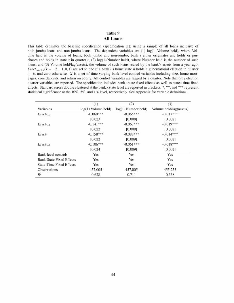
Table 9All Loans

This table estimates the baseline specification (specification (1)) using a sample of all loans inclusive ofboth jumbo loans and non-jumbo loans. The dependent variables are (1) log(1+Volume held), where Vol-ume held is the volume of loans, both jumbo and non-jumbo, bank i either originates and holds or pur-chases and holds in state s in quarter t, (2) log(1+Number held), where Number held is the number of suchloans, and (3) Volume held/lag(assets), the volume of such loans scaled by the bank’s assets from a year ago.Electi,h,t+k(k = −2,−1,0,1) are set to one if a bank i’s home state h holds a gubernatorial election in quartert + k, and zero otherwise. X is a set of time-varying bank-level control variables including size, home mort-gages, core deposits, and return on equity. All control variables are lagged by a quarter. Note that only electionquarter variables are reported. The specification includes bank×state fixed effects as well as state×time fixedeffects. Standard errors double clustered at the bank×state level are reported in brackets. *, **, and *** representstatistical significance at the 10%, 5%, and 1% level, respectively. See Appendix for variable definitions.

(1) (2) (3)Variables log(1+Volume held) log(1+Number held) Volume held/lag(assets)Electt−2 -0.069*** -0.065*** -0.017***

[0.023] [0.008] [0.002]Electt−1 -0.141*** -0.067*** -0.019***

[0.022] [0.008] [0.002]Electt -0.158*** -0.088*** -0.014***

[0.022] [0.009] [0.002]Electt+1 -0.106*** -0.061*** -0.018***

[0.024] [0.009] [0.002]Bank-level controls Yes Yes YesBank-State Fixed Effects Yes Yes YesState-Time Fixed Effects Yes Yes YesObservations 457,005 457,005 455,253R2 0.628 0.711 0.558

44

Table 10Robustness Checks

This table reports various robustness test results. Column (1) repeats our baseline regression (column (1) of table4) using pseudo-election dates where the election year is randomly selected for each state with a 4-year intervalexcluding the actual election year. Column (2) repeats our baseline regression excluding states which holdgubernatorial elections in the same year as presidential elections. Column (3) repeats the baseline specificationexcluding loans extended to three large states, California, New York, and Florida. The dependent variable islog(1+Volume held), where Volume held is the volume of jumbo loans bank i either originates and holds orpurchases and holds in state s in quarter t. Only election quarter variables are reported to save space. Standarderrors double clustered at the bank×state level are reported in brackets. *, **, and *** represent statisticalsignificance at the 10%, 5%, and 1% level, respectively. See Appendix for variable definitions.

(1) (2) (3)Pseudo-election Excluding states coinciding Excluding

Variables dates with pres. elections large statesElectt−2 0.025 -0.140** -0.124***

[0.030] [0.064] [0.037]Electt−1 0.111*** -0.268*** -0.205***

[0.029] [0.061] [0.035]Electt 0.031 -0.313*** -0.227***

[0.029] [0.062] [0.038]Electt+1 0.010 -0.150** -0.121***

[0.029] [0.067] [0.038]Bank-level controls Yes Yes YesBank-State Fixed Effects Yes Yes YesState-Time Fixed Effects Yes Yes YesObservations 207,535 170,536 184,842R2 0.574 0.570 0.565

45