1

POLITECNICO DI MILANO

POLO REGIONALE DI LECCO MASTER OF SCIENCE IN MECHANICAL ENGINEERING

DESIGN OF SUBSEA JUMPER & SPOOL PIPELINES

SUPERVISOR: PROF. GIORGIO PREVIATI

MASTER THESIS SUBMITTED BY LAURENT BERGER

MATRICOLA NUMBER: 801319

ACADEMIC YEAR 2013/2014

2

ABSTRACT :

In the past 40 years, subsea systems have advanced from shallow water, manually operated systems in Water Depth less than 1,000ft (305m), into systems capable of operating via remote control at water depth from 1,000ft up to 10,000 ft (3,000m). The design of the subsea components able to operate correctly in such extreme environment has become more and more complex because of the non-accessibility of the seabed. Multiple possibilities of locations and events have to be foreseen and tested. This thesis project aims at developing FEA design tools to compute automatically design models and to check international standards for Jumpers and Spools subsea pipelines. This mission was conducted in the Flowline Design Departement of the company SAIPEM SA Eni in Paris as an internship project. In this document, first of all, the usage of Jumpers and Spools among the subsea engineering system will be explained. Since those pipelines are usually designed in compliance with the international standards ASME B31.8 and DNV-OS-F101, a brief description of the different design load and stresses checks of those will be given. Then the complete range of components of Jumpers and Spools as well as the design conditions to be taken into account will be detailed. The life cycle of those structures, starting from the installation to the long term operations are be considered in the design. Eventually the Finite Element design spreadsheets developed will be explained. Both ABAQUS and AUTOPIPE software will be used to design Jumpers and Spools pipelines extracted from previous Saipem Eni projects. Verification and comparison of the results of stresses and reaction loads at the two bases will be used to validate the tool created for FE design of Jumpers and Spools. Jumpers and Spools design requires the consideration of multiple displacements cases corresponding to the different tolerances (installation and metrology) and multiple loading cases corresponding to the life cycle loads. Moreover the design of such an adaptable structure should be made in different geometrical configurations since the correct dimensions are only known at the very last step of installation. Taking into account the complete range of load cases is necessary for the design of the Jumpers and Spools . That’s the reason why an automatic VBA tool generating the input FE files and post-processing the outputs is useful for the Flowline Design Departement of Saipem SA. By reviewing the results obtained with the spreadsheets on both ABAQUS and AUTOPIPE, similar and comparable results are obtained, which indicates that models on both software are coherent. Safety margins ratios are computed and comply with international standards.

3

LIST OF FIGURES:

Figure 1. Typical subsea production systems ................................................................................................... 7 Figure 2. Typical offshore facilities .................................................................................................................... 8 Figure 3. Subsea Manifold and ROV ................................................................................................................. 8 Figure 4. Subsea PLET ..................................................................................................................................... 9 Figure 5. Typical manifold cluster layout ........................................................................................................... 9 Figure 6. Subsea steel umbilicals .................................................................................................................... 10 Figure 7. Vertical jumper.................................................................................................................................. 11 Figure 8. Rigid jumper installation ................................................................................................................... 11 Figure 9. Installation target boxes of two structures link by a Jumper ............................................................ 12 Figure 10. Two types of subsea Jumpers ........................................................................................................ 14 Figure 11 a & b. Vertical Tie In Jumper Installation ......................................................................................... 14 Figure 12. Horizontal Tie In Jumper ................................................................................................................ 15 Figure 13. Installation Procedure for a Horizontal Jumper .............................................................................. 15 Figure 14. Autopipe model of the connector extremity .................................................................................... 17 Figure 15. Abaqus model of the connector extremity ...................................................................................... 17 Figure 16. Wall thickness with bend thinning .................................................................................................. 19 Figure 17. Bend tubing manufacturing ............................................................................................................ 19 Figure 18. Epoxy coating ................................................................................................................................. 20 Figure 19. Pipe Cladding ................................................................................................................................. 20 Figure 20. Pipe Cross Section ......................................................................................................................... 20 Figure 24. Metrology drawing .......................................................................................................................... 22 Figure 25. Total length and elevation .............................................................................................................. 22 Figure 26. Hub orientation ............................................................................................................................... 22 Figure 21. Pre fabrication of a Jumper ............................................................................................................ 23 Figure 22. Shipping of a vertical jumper .......................................................................................................... 24 Figure 23. Lowering of the Vertical & Horizontal Jumpers .............................................................................. 24 Figure 27. US Shoe factory before and after the explosion ............................................................................ 26 Figure 28. Forces in pressurized pipeline ........................................................................................................ 28 Figure 29. Circumferential stress in a Pipeline pressurized Internally and Externally .................................... 29 Figure 30. Pipeline global buckling .................................................................................................................. 31 Figure 31. Buoys and Strakes for Jumpers ..................................................................................................... 32 Figure 32. Autopipe view, Jumper under gravity load & middle buoyancy ...................................................... 37 Figure 33. Autopipe view, Deformed shape jumper under gravity load .......................................................... 38 Figure 34. 3D Spool designed on Autopipe ..................................................................................................... 39 Figure 35. ASME Stress checks are performed by Autopipe .......................................................................... 39 Figure 36. Two nodes twelve degrees of freedom 3D pipe element ............................................................... 40 Figure 37. Beam orientation ............................................................................................................................ 42 Figure 38. Default integration, beam in space, thick pipe section ................................................................... 42 Figure 39. Default integration, beam in space, thin pipe section .................................................................... 42 Figure 40. 3D bend Mesh with Shell Elements ............................................................................................... 43 Figure 41. 3D bend Mesh with Brick Elements ............................................................................................... 43 Figure 42. Brick vs Shell Comparaison - Results for thin pipes ...................................................................... 43 Figure 43. Brick vs Shell Comparaison - Results for thick pipes ..................................................................... 44 Figure 44. Jumper with an imposed displacement on ABAQUS ..................................................................... 44 Figure 45. Input Spreadsheet .......................................................................................................................... 50 Figure 46. Jumper Dimensions ........................................................................................................................ 52 Figure 47. Typical Cumulative Probability ....................................................................................................... 56 Figure 48. Screenshot worksheet "INPUT" 3.0 CALCULATION part before loading data .............................. 59 Figure 49. Screenshot worksheet "INPUT" 3.0 CALCULATION part after loading data ................................. 59 Figure 50. Screenshot Abaqus command windows, the solver begins to run ................................................. 60 Figure 51. Screenshot Autopipe command windows, the solver begins to run............................................... 61 Figure 52. Bonga Northwest Field Layout ....................................................................................................... 73 Figure 53. Input Spreadsheet Bonga NorthWest ............................................................................................ 74 Figure 54. Abaqus model of Bonga Northwest ................................................................................................ 79 Figure 55. Bend close up in load case GRT27U ............................................................................................. 79

4

LIST OF TABLES:

Table 1. Example of connector load capacities ............................................................................................... 17 Table 2. Percentage Effect of Strengthening Mechanism ............................................................................... 17 Table 3. Typical Composition of Mn-Steels ..................................................................................................... 18 Table 4. Coating 3LPP..................................................................................................................................... 19 Table 5. Measuring Techniques and Accuracy ............................................................................................... 21 Table 6. Measurement tolerances ................................................................................................................... 21 Table 7. Design factor for Hoop, Longitudinal and Combined Stresses ......................................................... 29 Table 8. Temperature Derating Factor ............................................................................................................ 29 Table 9. Load Effect factor and Load Combination ......................................................................................... 34 Table 10. Condition Load Effect Factors ......................................................................................................... 34 Table 11. Material Resistance Factor .............................................................................................................. 34 Table 12. Safety Class Resistance Factor ...................................................................................................... 34

5

1. INTRODUCTION .............................................................................................................................................. 7

1.1 OVERVIEW OF SUBSEA PIPING STRUCTURES ..................................................................................................... 7 1.1.1 Subsea Manifolds ..................................................................................................................................... 8 1.1.2 Pipeline Ends and In-line Structures ..................................................................................................... 8 1.1.3 Subsea wellheads .................................................................................................................................... 9 1.1.4 Subsea Trees............................................................................................................................................ 9 1.1.5 Umbilical systems .................................................................................................................................. 10 1.1.6 Production risers .................................................................................................................................... 10 1.1.7 Subsea pipelines .................................................................................................................................... 10 1.1.8 Jumpers & Spools .................................................................................................................................. 10

1.2 PURPOSE OF THE THESIS ................................................................................................................................. 13

2. STATE OF THE ART ......................................................................................................................................14

2.1 BASIC COMPONENTS OF JUMPERS & SPOOLS .................................................................................................. 14 2.1.1 Jumper & Spool types ........................................................................................................................... 14

2.1.1.1 Vertical Tie-in ........................................................................................................................................................14 2.1.1.2 Horizontal Tie-in ...................................................................................................................................................15

2.1.2 Connectors .............................................................................................................................................. 16 2.1.3 Pipe Material ........................................................................................................................................... 17 2.1.4 Pipe components .................................................................................................................................... 19

2.2 METROLOGY ..................................................................................................................................................... 21 2.3 LIFE CYCLE ........................................................................................................................................................ 23

2.3.1 Transportation & Installation of Jumpers and Spools ....................................................................... 23 2.3.2 Stroking .................................................................................................................................................... 24 2.3.3 Offshore Hydrotest & Leak Test ........................................................................................................... 24 2.3.4 Design and Operating ............................................................................................................................ 25 2.3.5 Shut Down ............................................................................................................................................... 25 2.3.6 Retrieval ................................................................................................................................................... 25

2.4 DESIGN GUIDELINES ......................................................................................................................................... 25

3. DESIGN REQUIREMENTS FOR SPOOLS AND JUMPERS ......................................................................25

3.1 INTERNATIONAL PIPING STANDARDS ............................................................................................................... 25 3.1.1 ASME B31 Standards of Pressure Piping .......................................................................................... 26

3.1.1.1 History of ASME code .........................................................................................................................................26 3.1.1.1 Outline of Section VIII ASME B31.8 ..................................................................................................................26

3.1.1.1.1 Hoop Stress .....................................................................................................................................................27 3.1.1.1.2 Longitudinal Stress .........................................................................................................................................29 3.1.1.1.3 Combined Stress ............................................................................................................................................30

3.1.1.2 Loads considered for Spools and Jumpers Design .........................................................................................32 3.1.2 DNV, Det Norske Veritas ...................................................................................................................... 33

3.1.2.1 History of DNV code ............................................................................................................................................33 3.1.2.2 Outline of Pressure Piping ..................................................................................................................................33

4. THESIS ACTIVITY DESCRIPTION: JUMPERS & SPOOLS FEA DESIGN SPREADSHEETS ..............37

4.1 AUTOPIPE & ABAQUS FEA NUMERICAL MODELS............................................................................................... 37 4.1.1 AUTOPIPE .............................................................................................................................................. 37 4.1.2 ABAQUS .................................................................................................................................................. 40

4.2 INPUT SPREADSHEET ........................................................................................................................................ 46 4.2.1 Process Flowchart .................................................................................................................................. 58 4.2.2 Launching and Results .......................................................................................................................... 59 4.2.3 Abaqus Files ........................................................................................................................................... 60 4.2.4 Autopipe Files ......................................................................................................................................... 61

4.3 POST PROCESSING SPREADSHEETS ................................................................................................................ 61 4.3.1 Process Flowchart .................................................................................................................................. 72

5. RESULTS AND STUDY CASE ......................................................................................................................73

5.1 12” WATER INJECTION JUMPER : BONGA NORTHWEST, SHELL NIGERIA PRODUCTION ................................... 73

6. CONCLUSION .................................................................................................................................................80

6

ACKNOWLEDGEMENTS :

I would like to thank my kind company manager at SAIPEM SA, Engineer Simon Grevet for his full support throughout the entire duration of the project. Special thanks to my supervisor at Politecnico di Milano, Professor Giorgio Previati who gave me the opportunity of attending the Advanced Design course at Lecco, which has been of great help to comprehend Finite Element Analysis. Thoughts also go for parents, family and friends for their constant support.

7

1. INTRODUCTION

The introduction section deals with basics of subsea piping engineering in the oil and gas field. Spool and Jumper structures will be more deeply studied.

1.1 OVERVIEW OF SUBSEA PIPING STRUCTURES

The offshore oil and gas industry started in 1947 when Kerr-McGee completed the first successful offshore well in the Gulf of Mexico off Louisiana in 15 ft (4.6m) of water. The concept of subsea field development was suggested in the early 1970s by placing wellhead and production equipment on the seabed. The hydrocarbon produced would then flow from the well to a nearby processing facility, either on land or an existing offshore platform. This concept was the start of subsea engineering, and systems that have a well and associated equipment below the water surface are referred as subsea production systems.

Figure 1. Typical subsea production systems

The extracted oil or natural gas is transported by pipeline under the sea before it rises to a processing facility. The development of new fields can either be initiated via long tie-back to an existing facility or by installing a new “stand-alone” facility. The top side stand alone facilities can be divided into four typical host facilities : Floating Production Systems (FPS), Tension Leg platforms (TLP), Jack-up platform and semi-submersible platforms. -Floating Production Systems (FPS) : FP consist of large monohull structures, generally in the shape of ships, equipped with processing facilities. -Tension leg platforms (TLPs) : TLPs are floating platforms tethered to the seabed so that most vertical movement are eliminated. TLPs are used in water depths up to 2000m. -Jack-up platforms: Jack-up platforms are platforms that can be jacked up above the sea using legs that can be lowered. They are used up to around 150m water depth. -Semi-submersible platforms : These platforms have buoyancy modules to cause the structure to float and stay upright. Those installations can be used in water depth from 60 to 3050m.

8

Figure 2. Typical offshore facilities

The subsea production system consists of all the components and pipelines that ensure the transport of the oil and gas from the well to the facility. The different mechanical structures involve in a subsea production system are:

1.1.1 Subsea Manifolds

The manifold, as shown as in Figure 3, is an arrangement of piping and/or valves design to combine, distribute, control, and often monitor fluid flow. The manifold may be anchored to the seabed with piles or skirts that penetrate the mudline. The numerous types of manifold range from a simple Pipeline End Manifold (PLEM/PLET) to large structures such as a subsea process system.

Figure 3. Subsea Manifold and ROV

1.1.2 Pipeline Ends and In-line Structures

As the oil/gas field developments move further away from existing subsea infrastructures, it becomes advantageous to consider a subsea tie-in of their export systems. This requires incorporation of pipeline end manifolds (PLEMS) at both pipeline ends to tie-in the system. A PLEM is used to connect rigid pipeline with other subsea structure, such as manifold or tree, through a jumper. It is also called Pipeline End Termination (PLET). Figure 4 shows a typical subsea PLET.

9

Figure 4. Subsea PLET

1.1.3 Subsea wellheads

Wellhead is a general term used to describe the pressure-containing device at the surface of an oil well that provides the inferface for drilling, completion, and testing of all subsea operation phases. Subsea wells can be either satellite wells or clustered wells.

Satellite Wells are individual and remotely located to other wells. The primary advantage of satellite well is the flexibility of individual well exploitation. The production and treatment of each well can be optimized to the maximum.

Clustered Wells mean the gathering of several wells and the sharing of common facilities by those wells. This will then require fewer flowline and umbilicals, thus reducing costs. Clustered systems, however, introduce the need for subsea chokes to allow individual well control. Moreover the drilling operations of one well can interrupt production from the other.

Figure 5. Typical manifold cluster layout

Artificial lift methods are used to continuously remove liquids from a liquid loaded gas well. The lack of energy in a reservoir can affect the flow rate of oil, gas or water. Using this method, energy is transferred downhole and the fluid density in the wellbore is reduced.

1.1.4 Subsea Trees

The subsea production tree is an arrangement of valves, pipes, fittings, and connections placed on the top of a wellbore. Orientation of the valves can be vertical or horizontal and operated whether by electrical or hydraulic signals or manually by a driver or Remote Operated Vehicle (ROV).

10

1.1.5 Umbilical systems

An umbilical is bundled arrangement of tubing, piping, and/or electrical conductor in an armored sheath. It is used to transport control fluid and electrical current necessary to control the facilities. Dedicated tubes in an umbilical are used to monitor pressures and inject fluids from the host facility to critical areas within the subsea production equipments.

Figure 6. Subsea steel umbilicals

1.1.6 Production risers

The production riser is the portion of the flowline that resides between the host facility and the seabed adjacent to a host facility. Risers can be flexible or rigid. Those structure enable the rise of the production fluids to the surface facilities.

1.1.7 Subsea pipelines

Subsea flowlines are the subsea pipelines used to connect a subsea wellhead with a manifold or the surface facility. They may transport petrochemicals, lift gas, injection water and chemicals. A distinction can be made between the infield pipelines (typical range of 4”/12”) and the export pipelines that export the product from the field to onshore and to another facility (typical range 16”/36”). The flowlines may be made of flexible pipe or rigid pipe. Subsea pipelines are increasingly required to operate at high pressures and temperatures. The higher pressure condition results in the technical challenge of providing a higher material grade of pipe for and the HT will cause the challenges of corrosion, down-rated yield strength, and insulation coatings. Flowlines will be subjected to high effective axial compressive force due to the high fluid temperature and internal pressure causing expansion which is partially restrained by soil friction/in-line structures. Consequently, in the design process, the expansions of the lines have to be considered and propagated to the adjacent structures. Jumpers and Spools pipes are specially conceived to accommodate such expansions, thus preventing the propagation of the displacement to all the structures.

1.1.8 Jumpers & Spools

A Spool is a prefabricated short pipe connector used to transport production fluid between two subsea components. A Jumper is a Spool with vertical geometry either in 2D/3D that usually presents floatability (no contact with the seabed).

11

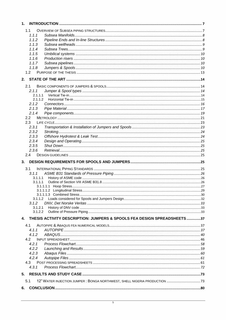
Figure 7. Vertical jumper

Such pipes are designed to accommodate installation tolerances and expansions of production lines. Jumpers and Spools primary purpose is to compensate the installation misalignments and line expansions during operations. Indeed those structures are the last equipment installed at the seabed and their special geometry provides flexibility and adaptability. Economically speaking, the most critical issue about Jumpers and Spools is the very short time available for fabrication works. The exact required dimensions of the structure are known only once all the other subsea production systems have been installed and metrology survey conducted. Since offshore installation implies high cost and involves expensive boats and crews, the fabrication time has to be controlled. That is the reason why studies of possible design options and pre-fabrication are important. It is essential to understand that most subsea structures are built onshore and transported to the offshore installation site. The installation includes three phases: lowering, landing and locking with the other structures.

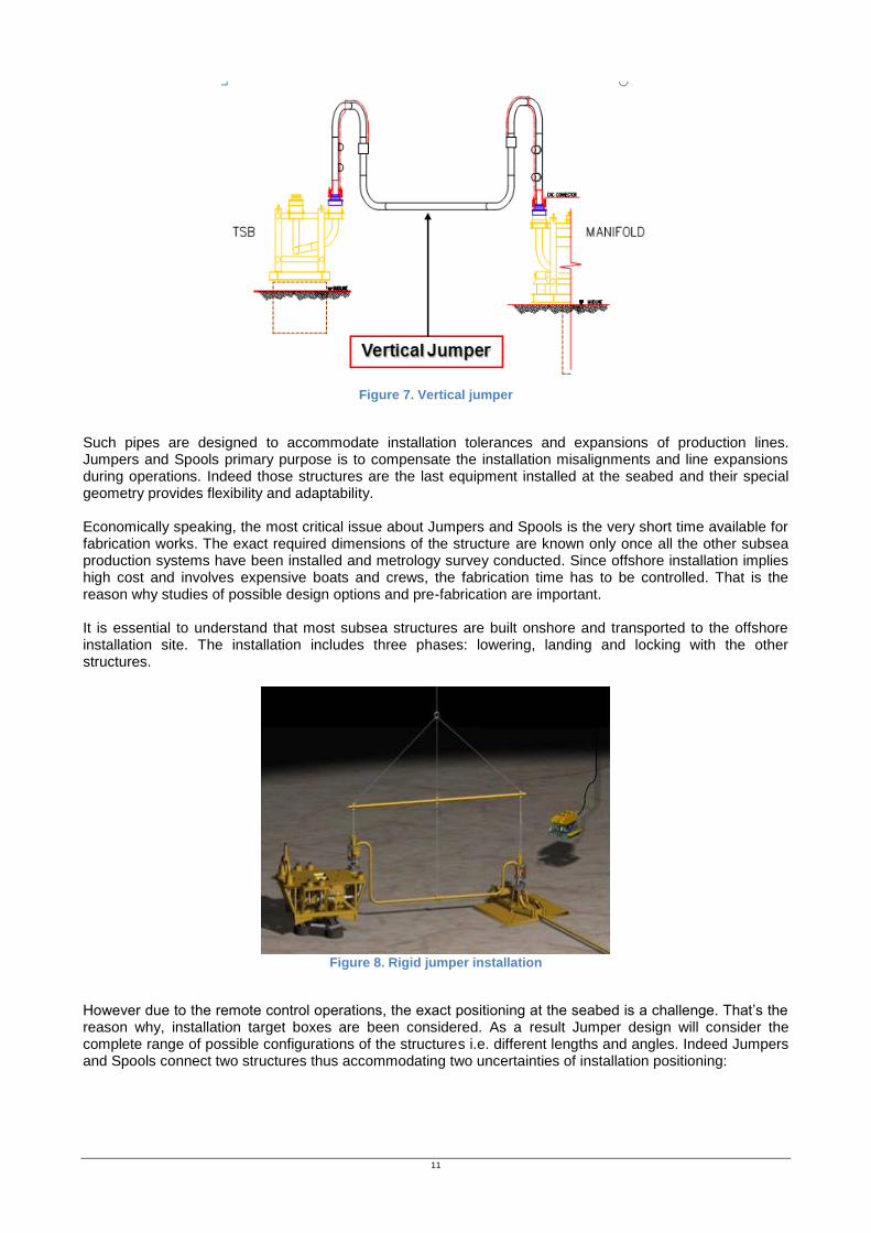
Figure 8. Rigid jumper installation

However due to the remote control operations, the exact positioning at the seabed is a challenge. That’s the reason why, installation target boxes are been considered. As a result Jumper design will consider the complete range of possible configurations of the structures i.e. different lengths and angles. Indeed Jumpers and Spools connect two structures thus accommodating two uncertainties of installation positioning:

12

Figure 9. Installation target boxes of two structures link by a Jumper

The strength studies of Jumpers & Spools require taking into account the geometry, the connecting ends, environmental loads and influences of the operating fluid. Thus Finite Element Analysis software are used to conduct appropriate design checks. International codes and standards are being applied for all the subsea systems. The main objective of those codes is to establish minimum requirements that are necessary for safe construction and operation. The client approval and design check of the subsea equipment are based on the adequacy with the standards (ASME, DNV). As a consequence a piping engineer must have a good understanding of the offshore section of those codes.

13

1.2 PURPOSE OF THE THESIS

The aim of this thesis is to study and model Jumpers & Spools for multiple projects developing automatic modeling FEA tools and post-processing in compliance with ASME B31.8. and DNV OS-F101 codes. The available software to model and analysis the structures are Bentley AUTOPIPE V8i Plus and ABAQUS v.6.12.1. The codes and standards should be respected and both FEA sofware should carry on design calculations. The difference between the two programs is that since ABAQUS is a general FEM software, the program is not able to perform directly the checks according to ASME B31.8 or DNV. Consequently calculations will have to be performed starting from the force and moment outputs of ABAQUS. However AUTOPIPE can present the outputs directly according to the standards in the case of ASME checks (Hoop stress, Longitudinal stress, Combined stress), but post processing is still necessary for DNV checks. The model philosophy is to generate the Jumper and Spool geometries with Pipes and Bends elements by automatic VBA code. All the components of those structures will be considered (connectors, coatings, claddings). All the elements are not exactly modeled but rather included in the design (for example coating and cladding are just represented by extra weight). Additionally the external loads (pressures, waves, buoyancy modules) on the structures as well as the imposed displacements at the extremities will be applied. Stresses and Reactions forces are to be summarized in order to perform the standard stress checks and connector load limits. Moreover the maximum displacements have to be assessed making available the seabed clearance of the structures. Jumpers & Spools design requires to test multiple geometrical configurations (Near-Near, Far-Far, Nominal, Positive angle, Negative angle) and multiple life-cycle steps (as landed, stroking, hydrotest, leak test, design, operating, shut-down, retrieval). Consequently tools developed are focusing on the “self-running” of the modeling and checking of all the configurations. The main objective of such tool is to increase the efficiency and reliability of Jumper & Spool design procedures. Both M-shaped Jumpers and three dimensional (3D) Spools will be designed and post processed. The soil contact, the buoyancy forces and the wave loads will make the design process more complex. In the next chapters, Jumpers and Spools will be modeled in details with both software and the results will be compared to ensure their validity. The project has been possible thanks to a tight planning of the different development steps. Indeed the approach of the subsea engineering and its understanding was the first required step of the study. Researching and reading the available documents about the design of subsea structures and redacting a technical memo that deals with the design of Jumpers and Spools represented the first task of the project. Creating coherent Abaqus models of Jumpers and Spools have been the second step of the project. Autopipe analysis have also been conducted in parallel in order to build comparison grounds. The post processing of both the FEA models has shown similarities. It has been the basis for the comprehension of the correct design of Jumpers and Spools in terms of geometry and loads. The development of automated spreadsheets generating input FEA files for models on both Abaqus and Autopipe and post-processing the outputs constitutes the very main innovating part of the project. Indeed the advantages of VBA coding have been exploited thus enabling the user of the newly developed spreadsheets to design multiple Jumpers (configurations) in multiple load cases (As Landed, Hydrotest, Leak Test, Operating, Design and Shut Down). At first, focus has been set on the design of vertical M-shaped Jumpers. Three spreadsheets which generate models with buoyancy modules and complete parameterized conditions (dimensions, pressure and temperature, loads) and post-process the outputs, have been created. The validation of those spreadsheets is being carried on internally in the Flowline Design Department of Saipem Eni, Paris. The Second step aims at improving the previously developed spreadsheets for M-shaped vertical Jumpers into 3D modeling of Jumpers/Spools. Very conclusive solutions for the modelling of 3D Jumpers have been reached during the thesis project and first versions of input spreadsheets have been issued. Testing and approvals of those spreadsheets are currently being conducted in the design department.

14

2. STATE OF THE ART

2.1 BASIC COMPONENTS OF JUMPERS & SPOOLS

The project has the objective of modelling Jumpers and Spools of subsea projects and to analyze those structures on FEA software. In order to correctly define those pipelines, it is necessary to understand all different types of Jumpers and Spools that can be encountered and their components.

2.1.1 Jumper & Spool types

A typical jumper consists of two ends connectors and a pipe between the two connectors. If the pipe is a rigid pipe, the jumper is a rigid jumper. If the pipe is flexible, the jumper is a flexible jumper. In this thesis only rigid jumpers have been studied. Jumper configurations are dictated by design parameters, interfaces with subsea equipment, and the different modes in which the jumper will operate. Two types of configurations can be distinguished: the vertical tie-in and the horizontal tie-in.

Figure 10. Two types of subsea Jumpers

2.1.1.1 Vertical Tie-in

Vertical jumpers, are typical vertical tie-in systems and use mechanical collet connectors at each end. The connection at the extremities of the jumper pipe is made possible thanks to connector hub. The stroking and connection are carried out by the connector itself, or by ROV (Remote Operated Vehicle)-operated connector actuation tool (CAT) as shown in Figure 11. Advantages of vertical configuration are the faster connection process and the less demanding requirement of pipe length. However the complex transportation of those structures and the high weather dependence installation with the required advanced connector technology may counter balance the advantages.

Figure 11 a & b. Vertical Tie In Jumper Installation

15

2.1.1.2 Horizontal Tie-in

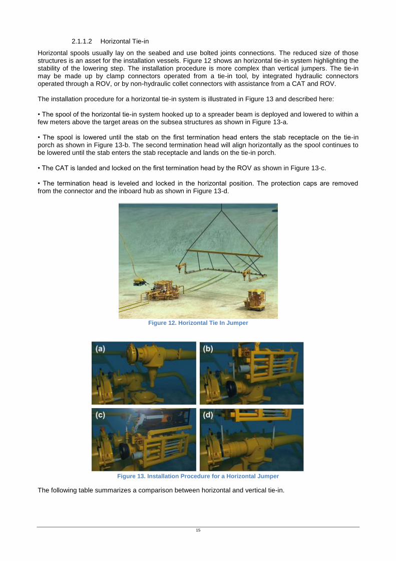
Horizontal spools usually lay on the seabed and use bolted joints connections. The reduced size of those structures is an asset for the installation vessels. Figure 12 shows an horizontal tie-in system highlighting the stability of the lowering step. The installation procedure is more complex than vertical jumpers. The tie-in may be made up by clamp connectors operated from a tie-in tool, by integrated hydraulic connectors operated through a ROV, or by non-hydraulic collet connectors with assistance from a CAT and ROV. The installation procedure for a horizontal tie-in system is illustrated in Figure 13 and described here: • The spool of the horizontal tie-in system hooked up to a spreader beam is deployed and lowered to within a few meters above the target areas on the subsea structures as shown in Figure 13-a. • The spool is lowered until the stab on the first termination head enters the stab receptacle on the tie-in porch as shown in Figure 13-b. The second termination head will align horizontally as the spool continues to be lowered until the stab enters the stab receptacle and lands on the tie-in porch. • The CAT is landed and locked on the first termination head by the ROV as shown in Figure 13-c. • The termination head is leveled and locked in the horizontal position. The protection caps are removed from the connector and the inboard hub as shown in Figure 13-d.

Figure 12. Horizontal Tie In Jumper

Figure 13. Installation Procedure for a Horizontal Jumper

The following table summarizes a comparison between horizontal and vertical tie-in.

16

Both types of tie-in can be encountered and models for both are developed. The geometry generating tools will be modified accordingly. The type of Jumper/Spool will have significant impact on adjacent structures: the connectors, settlement and interfaces will be different. The horizontal type would impose coordinate transformation at the extremities to deliver correct reaction loads (forces and moments). Indeed the reactions loads are part of the check demanded by the design procedures since connector manufacturers give maximum allowable loads that can be applied on the connector hubs.

2.1.2 Connectors

The connector should be used at the end of the jumper piping to lock and seal the mating hub on the connector receiver. The connector should be equipped with the following components: (1) a mechanism (e.g., collet, fingers, or dogs) designed to resist lateral and longitudinal forces that may be encountered in the process of aligning and final lowering, prior to makeup of the connection (the connector is designed to accommodate the design loads); (2) metal-to-metal seal surfaces inlaid with corrosion resistant alloy; the seal surfaces shall be relatively insensitive to contaminants or minor surface defects and maintain seal integrity in the presence of the maximum bending moments and/or torsional moments; (3) a metal seal with an elastomeric backup capable of multiple makeups; (4) mechanical position indicators to indicate lock/unlock operations that are clearly readable by an ROV; (5) a mechanical release override or a hydraulic secondary release system. The connectors will be modelled by a hub-pipe with rigid properties. Indeed the connector hub can be considered much more rigid compared to the jumper pipe. Moreover the submerged weight of the connector will be applied at the hub middle length. Pup piece length can also be added in the design model as an extra pipe length with similar properties to the jumper pipe. In both models developed for Abaqus and Autopipe, the length of the hub and the pup piece are parameterized. Indeed each project will present a different configuration.

17

Figure 15. Abaqus model of the connector extremity

The connectors have allowable loads. Indeed the envelope values corresponding to maximum shear force, vertical force, bending moment and torsion on the connector have to be respected in compliance with the manufacturer specifications. Here below is an example of connector capacities for a CAMERON 12” connector.

Table 1. Example of connector load capacities

2.1.3 Pipe Material

Pipe steels must perform in a harsh environment, subject to the many corrosive and erosive actions of the sea, under dynamic cyclic and impact conditions over a wide range of temperatures. Thus, special criteria and requirements are imposed on the material qualities and their control. A pipeline steel must have high strength while retaining ductibility, fracture toughness, and weldability. -Strength is the ability of the pipe steel (and welds) to resist the longitudinal and transverse tensile forces imposed on the pipe. -Ductibility is the ability of the pipe to absorb overstressing by deformation. -Toughness is the ability of the pipe material to withstand impacts or shock loads. -Weldability is the ability to ease the production of quality welds and heat-affected zones of adequate strength and toughness. For submarine pipelines, the prime factor driving the need for good weldability is economic. The faster the pipe can be welded, the faster it can be installed and the shorter the period of use of lay barge (high cost associated with lay barge use). The steel used to form pipe joints are low carbon-manganese steels. This composition is offering the best comprise in terms of strength, reduction in tonnage and weldability. Table 7 below shows the typical strengthening processes for API 5L type pipeline steel with 1.5% manganese.

Table 2. Percentage Effect of Strengthening Mechanism

The higher strength grades are microalloyed and may be referred to as high-strength low-alloy (HSLA) steels. The pipe joints for oil and gas will conform to the American Petroleum Institute API Specification 5L.

Figure 14. Autopipe model of the connector extremity

18

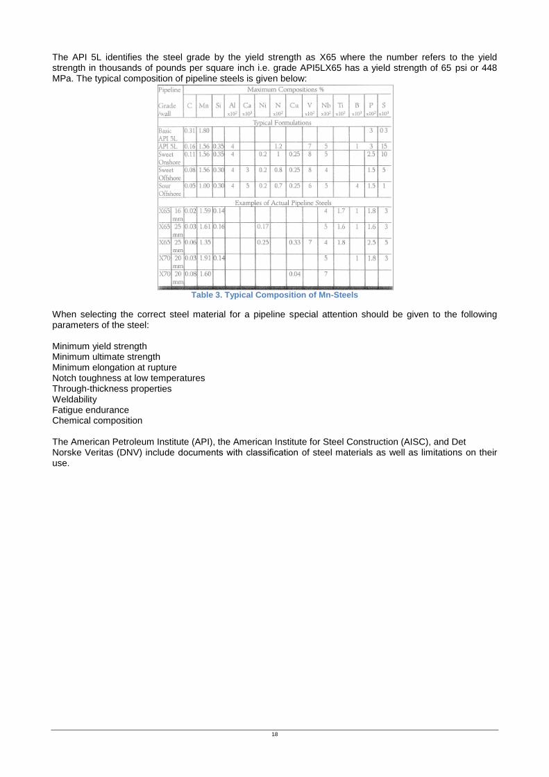
The API 5L identifies the steel grade by the yield strength as X65 where the number refers to the yield strength in thousands of pounds per square inch i.e. grade API5LX65 has a yield strength of 65 psi or 448 MPa. The typical composition of pipeline steels is given below:

Table 3. Typical Composition of Mn-Steels

When selecting the correct steel material for a pipeline special attention should be given to the following parameters of the steel: Minimum yield strength Minimum ultimate strength Minimum elongation at rupture Notch toughness at low temperatures Through-thickness properties Weldability Fatigue endurance Chemical composition The American Petroleum Institute (API), the American Institute for Steel Construction (AISC), and Det Norske Veritas (DNV) include documents with classification of steel materials as well as limitations on their use.

19

2.1.4 Pipe components

The Outside diameter (OD) of the jumper pipe should be known. Usually indicated in inch it should be converted into mm if required. The bend radius of the structure is also an important parameter as it should be well designed to comply with the applied stress but also to assure correct flow of the product content. Moreover the bend radius is constrained by the circulation of testing/cleaning devices (Pigs) that travel the pipe. In the bend sections, the thickness is usually reduced because of the fabrication process that consists in bending a formerly straight pipe. When tubing is bent, the wall of the outside edge of the curve stretches and becomes thinner, while the wall of the inside edge compresses and becomes thicker. If the walls of tubing are too thin to begin with, the outside edge will break, kink, or deform. Consequently a bend thinning percentage should be applied to the wall thickness in the calculation of the stress in the bend. The Ovality induced by the fabrication of the bended pipe should also be considered.

Figure 16. Wall thickness with bend thinning

Figure 17. Bend tubing manufacturing

The Wall Thickness (WT) is also determined according to the difference of pressure applied to the pipe between outside and inside. The Corrosion Allowance (CA) is an estimated corrosion thickness that could be deducted from the nominal thickness in case of corrosion. The nominal thickness (WT) is theoretically known however a fabrication tolerance should be taken into account. Coating of the pipe is carried on to ensure excellent resistance to corrosion, abrasive wear and tear. Three Layer Polypropylene Coating (3LPP) is usually used as anti-corrosion coating. The weight of the coating must be taken into account in the design of the Jumpers and Spools. Here below is an example of the 3LPP coating data.

Table 4. Coating 3LPP

Insulation thickness required to prevent hydrate formation during operations (obstruction of the flow) and to maintain a certain fluid temperature may also be part of the properties of the pipe.

20

Figure 18. Epoxy coating

Cladding can sometimes be used in case of particularly severe corrosive conditions of the product content. It is a coating of high-cost corrosion resistant alloys applied on the pipe inner surface. Weld overlay cladding of carbon steel offers a wide choice of processes and flexibility to protect an almost infinite range of component shapes and sizes, with an equally wide range of base materials and cladding alloys.

Figure 19. Pipe Cladding

The drawing below represents a cross-section of the Jumper/Spool pipe :

Figure 20. Pipe Cross Section

The pipe will be submitted to different loading conditions (variation in internal pressure, product content and related density). Indeed the installation steps during which the jumper is flooded needs to be studied. Then testing phases of the installation with water content but at higher pressure are part of the process. Finally operating conditions with product content happen. The design process should also be aware of the exceptional possible shut down state (no content is left in the pipe) and retrieval operations.

21

2.2 METROLOGY

The structures are equipped with transponders. During the survey campaign, after installation of structures to connect with jumpers (PLETs, FLETs, SOMs, Manifolds), precise positioning of the equipment is measured. From the vessel, we measure the exact coordinates and orientation of the installed hubs. Several measuring techniques are used, as shown in the table below, the accuracies of the results are also taken into account.

Table 5. Measuring Techniques and Accuracy

For the design process an angular and a linear tolerance which include both the metrology tolerance and the fabrication tolerance are defined.

Table 6. Measurement tolerances

Typical drawings obtained after metrology enable the designer to collect data about the length and orientation of the hubs.

22

Figure 21. Metrology drawing

The interesting data to extract from this drawing are : - Total Length between the 2 hubs and elevations.

Figure 22. Total length and elevation

-The headings of each hub.

Figure 23. Hub orientation

23

2.3 LIFE CYCLE

The following flowchart represents the different steps in the jumper life cycle.

Content density, pressure conditions, temperature conditions will vary during the steps described above. Consequently the model that has to be created is going to consider each of those life cycle steps.

2.3.1 Transportation & Installation of Jumpers and Spools

The Jumpers and Spools are pre-fabricated. They are usually composed of: - 2 connectors with their pup-pieces - 2 vertical U-shape parts - 2 horizontal parts

Figure 24. Pre fabrication of a Jumper

After the subsea hardware is installed, the distances between the components to be connected are measured or calculated. Then the connecting jumper is fabricated to the actual subsea metrology for the corresponding hub on each component. Pipes are fabricated to the desired length and provided with coupling hubs on the ends for the connection between the two components. Once the jumper has been fabricated, it is transported to the offshore location for the deployment of subsea equipment. The jumper will be lowered to the seabed, locked onto the respective mating hubs, tested, and then commissioned. If the

Landing

Strocking

Offshore Hydrotest

Offshore Leak Test

Operating

Retrieval

Onshore Hydrotest

24

measurements have not been precisely made or the components moved from their originally planned locations, new jumpers may need to be fabricated.

Figure 25. Shipping of a vertical jumper

The distance and the orientation between the subsea components must be known in advance before the fabrication of flowline jumpers because the lengths will be critical. Also, a small change in the jumper configuration should be considered when the jumper is lowered below the water surface and the dead load of jumper changes due to the buoyancy: otherwise, the jumper’s dimensions may change and the jumper installation may fail. After the installation, if one of the components needs to be retrieved or moved, it is a time-consuming task to disconnect the flowline jumper from the component. Figure 22 shows a transportation/shipping stand with a rigid jumper on a barge. The transportation/Shipping stands are designed to comply with: • The stand should support the jumper in the installed configuration at the fabrication site or while en route to the installation site. • The stand should not limit connector operation and access. • It should have access ladders and work platforms if required • It should allow for welding down for transport of a jumper offshore • It should be designed to accommodate shipping of different jumper sizes. • It should use a guide funnel to facilitate installation of a jumper.

Figure 26. Lowering of the Vertical & Horizontal Jumpers

2.3.2 Stroking

The stroking is the operation that consists in the connection of the jumper ends with the connector structures. Indeed the mechanical collet in the horizontal configuration of Jumpers at the extremity implies the need for a compression of the extremities. This load will be considered in the model considered by an imposed displacement (in compression) at the extremities with a stroking length value.

2.3.3 Offshore Hydrotest & Leak Test

The Pre-Commissioning operations are to test the integrity of the lines and the jumper installed. Consequently higher pressure (1.25 times the operating pressure for the Hydrotest) with water content

25

flowing is applied to the lines. Pressure tightness can be tested by shutting off the supply valve and observing whether there is a pressure loss. Possible default in installation, material failure or leak can be detected with those tests. The design of the jumper will consider the cases of pre-commissioning activities considering the extra pressures in order to evaluate the stress induced in the Jumper and Spool structures. The line expansions of the Hydrotest and Leak test are applied on the jumper extremities.

2.3.4 Design and Operating

The Operating conditions are defined in accordance with the well content exploitation. The Maximum Allowable Operating Pressure (MAOP) is a design basis data. It corresponds to how much pressure of the well may safely hold in normal operation. Design pressure is the maximum pressure a pressurised item can be exposed to. Those pressures should constitute loading test of the structure and will be part of the conditions studied by the ABAQUS and AUTOPIPE models. The line expansions associated with the design and operating conditions should also be distinguished as they will impose displacements to the jumper extremities.

2.3.5 Shut Down

In case no content is flowed into the Jumper, the internal pressure will be very low compared to the external hydrostatic pressure. The Shut Down case considers that the internal pressure is zero. The complete shutdown of the well would entail such a situation. Comparing the stress range between the operating and the shutdown case is the basis for the evaluation of the fatigue life of the Jumper.

2.3.6 Retrieval

Finally the retrieval of the jumper, which corresponds to an inverse stroking (in the case of horizontal Jumpers), is to be tested. An extra imposed displacement at the extremities should be applied in the AUTOPIPE and ABAQUS models. This load case is not usually studied but it can be asked if the client company aims at retrieving the jumpers.

2.4 DESIGN GUIDELINES

Jumper length is defined according to the layout configuration. The target boxes of each end extremities allow the engineer to define Near-Near (NN), Far-Far (FF), Nominal (N), Near Near (NN), Worst Angle and Far Far Worst Angle (FFWA) configurations. The lengths of each configuration will be different and the angle with the existing lines will also differ. The Attachment E presents the jumper layouts used for the Bonga North West project conducted by Saipem in 2012. Due to allowable constraints, jumper height must change between configurations (NN – FF). A sensitivity can be performed to determine the cutoff for height vs hub-hub length to remain within allowable design envelopes. Indeed a longer jumper would not be able to stay within the limits if the loops heights are too important. However shorter jumpers can withstand higher loops. Buoyancies can also be added along the length of the Jumper. Usual places for settling buoyancy modules are the two vertical internal straights as well as the longer horizontal straight section. The buoyancy is modeled by concentrated upward vertical force with common values around 6000 kN. The buoyancies limit the deflection of the Jumper thus limiting the stress. Eventually the reaction loads at the extremities should be checked under the allowable loads for the connector’s hubs and adjacent structures. The shear force, the vertical force, the bending moment and the torsion must be into the allowable limits.

3. DESIGN REQUIREMENTS FOR SPOOLS AND JUMPERS

3.1 INTERNATIONAL PIPING STANDARDS

The subsea environment induces challenges for structure design: inaccessibility of the seabed, dynamic positioning and difficult accuracy of installation, high pressure and thermal loads, corrosion and scale, erosion and settlement of the structures at the seabed, water currents, flow assurance concern, dramatic costs of repair. Consequently the design of subsea structures is very demanding in terms of quality and respect of norms. That’s the reason why the industry follows the design rules of international codes. A pipeline clearly has to be strong enough to withstand all the loads that will be applied to it. It will be loaded by internal pressure from the fluid it carries, by external pressure from the sea, and by stresses induced by

26

temperature changes. Sometimes it will be loaded by external impacts from anchors and fishing gear. Two main code give recommendations for the design of pipes and subsea pipelines: the American Society of Mechanical Engineer (ASME) section B31, and the Det Norske Veritas (DNV).

3.1.1 ASME B31 Standards of Pressure Piping

ASME B31 covers Power Piping, Fuel Gas Piping, Process Piping, Pipeline Transportation Systems for Liquid Hydrocarbons and Other Liquids, Refrigeration Piping and Heat Transfer Components and Building Services Piping. ASME B31 was earlier known as ANSI B31.

3.1.1.1 History of ASME code

On March 20, 1905, a disastrous boiler explosion occurred in a shoe factory in Brockton, Massachusetts, killing 58 persons, injuring 117 others and causing a quarter of a million dollars in property damage.

Figure 27. US Shoe factory before and after the explosion

This catastrophic accident made the people of Massachusetts aware of the necessity of legislating rules and regulations for the construction of steam boilers in order to ensure their maximum safety. The state enacted the first legal code of rules for the construction of steam boilers in 1907. In 1908, the state of Ohio passed similar legislation, the Ohio board of boiler Rules adopting, with a few changes, the rules of the Massachusetts Board. Therefore, other states and cities in which explosions had taken place began to realize that accidents could be prevented by proper design, construction and inspection of boilers and pressure vessels and began to formulate rules and regulations for this purpose. As regulations differed from state to state and often conflicted with one another, manufacturers began to find it difficult to construct vessels for use in one state that would be accepted in another. Because of this lack of uniformity, both manufactures and users made an appeal in 1911 to Council of the American Society of Mechanical Engineers to correct the situation. The Council answered the appeal by appointing a committee ‘to formulate standard specifications for construction of steam boilers. The first committee consisted of seven members, all experts in their respective fields: one boiler insurance engineer, one material manufacturer, two boiler manufacturers, two professors of engineering and one consulting engineer. The committee was assisted by an advisory committee of 18 engineers representing various phases of design, construction, installation and operation of boilers. Following a thorough study of the Massachusetts and Ohio rules and other useful data, the committee made its preliminary report in 1913 and sent 2000 copies of it to professors of mechanical engineering, engineering departments of boiler insurance companies, chief inspectors of boiler inspection departments of states and cities, manufacturers of steam boilers, editors of engineering journals and others interested in the construction and operation of steam boilers, with a request for suggestions of changes or additions to the proposed regulations. After three years of countless meetings and public hearings, a final draft of the first ASME Rules for Construction of Stationary Boilers and for allowable Working Pressure, known as the 1914 edition, was adopted in spring of 1915.

3.1.1.1 Outline of Section VIII ASME B31.8

Section VIII of ASME B31.Ref[9] is dedicated to offshore gas transmission piping. This chapter is divided into:

-A801 General

27

-A802 Scope and intent

-A803 Offshore gas transmission terms and definitions

-A811 Qualification of materials and equipment

-A814 Material specifications

-A817 Conditions for the reuse and requalification of pipe

-A820 Welding offshore pipelines

-A823 Qualification of procedures and welders

-A825 Stress relieving

-A826 Inspection of welds

-A830 Piping system components and fabrication details

-A832 Expansion and flexibility

-A834 Support and anchorage for exposed piping

-A835 Anchorage for buried piping

-A840 Design, Installation, and testing

-A841 Design considerations

-A842 Strength considerations

-A843 Compressor stations

-A844 On-bottom stability

-A847 Testing

-A850 Operating and maintenance procedures affecting the safety of gas transmission facility

-A851 Pipeline maintenance

-A861 External corrosion control

-A864 Internal corrosion control

The stress equations and design factors are given in the part A842.Strength considerations. Both the steps of pipeline installation and pipeline operations should be studied with specific considerations.

During all phases of pipeline system installation (i.e. handling, laying, trenching and testing) the system should respect the minimum safety requirements against the following possible modes of failure: Design against yielding: When in operation, pressure and thermal forces act on the pipe, which tend to expand the pipeline both axially and longitudinally. These are due to internal pressure and temperature difference between the pipe and surrounding fluid.

3.1.1.1.1 Hoop Stress

Internal pressure from the contained fluid is the most important loading a pipeline has to carry. It is easy to forget how large the forces generated by pressure are. Figure28 shows a typical large diameter gas pipeline of 30in (0.762m) carrying an internal pressure of 15MPa. Half the pipe and half the contents are redrawn in Figure 29.b. pressing downwards on a 1 m length of this system is the pressure of the gas multiplied by the area over which it acts, a rectangle 0.75 m broad and 1m long. Pulling upwards on the same 1 m length is the tension in the pipe walls. There are no other vertical forces in a straight section of pipe. Since the system is in equilibrium, the tension in the pipe walls must be :

Which gives :

This value is 1100 tons, a substantial force, more than the take-off weight of three 747 aircrafts.

28

The hoop stress generated by internal pressure is statically determined, so that no significant stress redistribution can occur. If the hoop stress is too large, the pipeline can yield circumferentially and lead to rupture.

Figure 28. Forces in pressurized pipeline

A pipeline is a pressure vessel in the form of a cylinder, and, for this reason, some of the most detailed information available is obtained in the literature for pressure vessel design. Pipes with D/t greater than 30 are referred to as thin-wall pipes, and that with D/t less than 30 are called thick-wall pipes -The tensile hoop stress due to the difference between internal and external pressures should not exceed the value given below. Note : sign convention is such that tension is positive and compression negative.

Eq. (2) is used for D/t greater than or equal to 30; and Eq. (3) is used for D/t less than 30.

29

Figure 29. Circumferential stress in a Pipeline pressurized Internally and Externally

The design factor of the stress check equations are given in the Table A842.2.2-1 of the ASME B31.8 code.

Table 7. Design factor for Hoop, Longitudinal and Combined Stresses

The high temperature conditions have influence on the strength of the pipe material. Consequently Temperature Derating Factor is used to correct the equations of the codes.

Table 8. Temperature Derating Factor

3.1.1.1.2 Longitudinal Stress

A pipeline in operation carries longitudinal stress as well as hoop stress. Longitudinal stresses arise from two effects. First the Poisson effect: a bar loaded in tension extends in the tension direction and contracts transversely. If transverse contraction is prevented, a transverse tensile stress is set up. The analysis of hoop stress shows

30

that internal pressure induces circumferential tensile stress. If there were only circumferential stress and no longitudinal stress, the pipe would extend circumferentially (increase of diameter) but would contract longitudinally (shorter pipe). If friction against the seabed or attachment to fixed objects such as platforms prevents longitudinal contraction, a longitudinal tensile stress occurs. The second effect is temperature. If temperature of a pipeline increases and if the pipeline is free to expand in all direction, it expands both circumferentially and axially. Circumferential expansion is usually completely unconstrained, but longitudinal expansion is constrained by seabed friction and structures tied to the pipeline. It follows that if expansion is prevented, a longitudinal compressive stress will be induced in the pipe. Expansion stresses can be very large. the stress required to suppress uniaxial expansion completly under a temperature difference θ is where is the elastic modulus and α is the linear thermal expansion

coefficient. For steel, is 2.4 N/mm^2 degC, so that a temperature increase of 100° in a constrained situation induces a longitudinal stress of 240 MPa, which can be an important fraction of the yield strength. -The longitudinal stress shall not exceed the values found from:

With

3.1.1.1.3 Combined Stress

-The combined stress should not exceed the value given by the maximum shear stress equation (Tresca combined stress):

With

31

Alternatively, the Maximum Distortion Energy (Von Mises combined stress) may be used for limiting combined stress value:

As seen previously, the ASME B31.8 is based on allowable-stress design using the yield strength of the material. This approach is always conservative. Another method of design would be Limit-state design which consists on evaluating the critical loads that lead to failure and design the structures so that in operating mode it is always far from the failure condition. This approach would be less conservative since the structure would be allowed to reach yield point. Design against buckling: Theoretically, buckling is caused by a bifurcation in the solution to the equations of static equilibrium. At a certain stage under an increasing load, further load is able to be sustained in one of two states of equilibrium: an unstable un-deformed state or a stable laterally-deformed state. In practice, buckling is characterized by a sudden failure of a structural member subjected to high compressive stress, where the actual compressive stress at the point of failure is less than the ultimate compressive stresses that the material is capable of withstanding. Mathematical analysis of buckling often makes use of an axial load eccentricity that introduces a secondary bending moment, which is not a part of the primary applied forces to which the member is subjected. As an applied load is increased on a member, such as column, it will ultimately become large enough to cause the member to become unstable and is said to have buckled. Further load will cause significant and somewhat unpredictable deformations, possibly leading to complete loss of the member's load-carrying capacity. Moreover the pipelines are subjected to compression due to expansions, the force applied can trigger buckling of the line. Consequently avoidance of buckling of the pipeline shall be considered in the design.

Figure 30. Pipeline global buckling

Design against Fatigue: Stress fluctuations of sufficient magnitude and frequency which are susceptible to induce significant fatigue should be considered in design. Loading that may affect fatigue include:

a) Startup / Shut Down (Pressure and Temperature Cycles) The change in temperature and pressure conditions inside the pipeline induces fatigue loads. The expansions cycles due to temperature are causing such actions.

b) Waves actions

Wave loads being repetitive on the pipe, they can also trigger shorter fatigue life.

32

c) Vibration Induced by Vortex (VIV)

In fluid dynamics, vortex shedding is an oscillating flow that takes place when a fluid such as air or water flows past a cylindrical body. In this flow, vortices are created at the back of the body and detach periodically from either side of the body. If the cylindrical structure is not mounted rigidly and the frequency of vortex shedding matches the resonance frequency of the structure, the structure can begin to resonate, vibrating with harmonic oscillations driven by the energy of the flow. Vortex shedding was one of the causes proposed for the failure of the original Tacoma Narrows Bridge in 1940, but was rejected because the frequency of the vortex shedding did not match that of the bridge. The bridge actually failed by aeroelastic flutter. Pipelines spans should be designed so that Vortex Induced resonant Vibrations (VIV) are prevented. Nowadays the standard DNV code is a reference in term of fatigue life calculation. Pipeline Strakes are commonly used on Jumpers and Spools to introduce turbulence of the flow so that the load is less variable and resonant load frequencies have negligible amplitudes

Figure 31. Buoys and Strakes for Jumpers

Design against Fracture: Materials used for pipelines transporting gas or gas-liquid mixtures under high pressure should have reasonably high resistance to propagating fractures at the design conditions. Design of Clamps and Supports: Clamps and Supports shall be designed such that a smooth transfer of loads is made from the pipeline to the supported structure without highly focalized stress concentrations. The loads applied by the structure on each connector end will be checked and compared to the allowable loads of the connectors. Connectors and flanges shall have a level of safety against failure by yielding and failure by fatigue that is comparable to that of the attached pipeline. Design of structural pipeline: Where pipelines are installed in location subject to impact from marine traffic, protective devices shall be installed. Additional considerations include design storm currents, seabed movements, soil liquefaction, increased potential corrosion, thermal expansions and contraction.

3.1.1.2 Loads considered for Spools and Jumpers Design

A number of physical parameters, henceforth referred to as design conditions, govern design of the offshore pipeline systems so that it meets installation, operation, and other post installation requirements. The loads and factors that should be taken into account are: -pressure load: the differences of pressures whether it be in operations or in shut down configurations, will create important stresses.

33

-weight: the effect of pipe assembly weights (in air and submerged) as well as the variability due to weight coating tolerances and water absorption should be considered. -thermal expansions: expansions of the lines as well as the expansion of the jumper itself due to thermal loads shall be taken into account for the design of the structures. Those expansions are modelled by imposed displacements at the extremities of the structure. -linear and angular tolerances: metrology and installation tolerances shall be tested in advance to the installation procedure in order to ensure the conservatism of the solutions chosen whatever the configuration is at the time of the installation. -buoyancy: the action of buoyancy modules shall be modeled as they are used to relieve the jumper/spool from the bending moments due to self-weight. -wave actions: current velocity with the drag and lift effect should be applied on the structure. Additionally studies of the Vortex Induced Vibrations and fatigue life have to be conducted. -marine soil: if contact happens the model should be accordingly configured with the friction coefficients of the soil. -support settlement: both the initial settlement and the long-term settlement of the end structures will have influence on the jumper behavior.

3.1.2 DNV, Det Norske Veritas

3.1.2.1 History of DNV code

DNV was organized as a foundation, with the objective of "Safeguarding life, property, and the environment". The organization's history goes back to 1864, when the foundation was established in Norway to inspect and evaluate the technical condition of Norwegian merchant vessels. The foundation is oraganized into 3 corporations: DNV Maritime and Oil & Gas, DNV KEMA Energy & Sustainability, DNV Business Assurance.

3.1.2.2 Outline of Pressure Piping

The design of Jumpers with the prime design code DNV OS-F101 is based on Load and Resistance Factor Design (LRFD) which ensured a satisfactory level of safety when the design load effect does not exceed the design resistance.

The jumper bends are also required to satisfy the requirement for combined loading local buckling. In addition, all the bends shall be checked using Allowable Stress Design (ASD) in accordance with DNV OS-F-101, Section 5 F200.

The fundamental principle of the Load and Resistance Factor Design (LRFD) format is that design load effects, Lsd, do not exceed design resistances, Rrd, for any of the considered failure modes in any load scenario:

Where

The design load effect can generally be expressed as :

Where Lf, Le, Li and La are the functional, environmental, interference and accidental loads. The function load corresponds to the pressure and temperature conditions while the environmental loads are considering the wave actions. The interference loads are modelling the loads induced by dropping objects on the pipes or fishing tools. In specific forms, this corresponds to :

34

Where Msd, Esd, Ssd are the design moment, design strain and design effective axial force. The coefficients ɣF, ɣE, ɣA are the functional, environemental and accidental load factors and ɣC the load condition factor. They are given in the following table.

Table 9. Load Effect factor and Load Combination

Table 10. Condition Load Effect Factors

The relevant limit states (failures modes) are: Serviceability Limit State Category (SLS), Ultimate Limit State Category (ULS), Fatigue Limit States (FLS) and Accidental Limit State (ALS).

The design resistance is generally expressed as :

Where

Two different characterisations of the wall thickness tc are used : t1 and t2. Thickness t1 is used where failure is likely to occur in connection with a low capacity while thickness t2 is used when failure is likely to occur with an extreme load effect.

The material resistance factor, , is dependent on the limit state category and is defined in the following table :

Table 11. Material Resistance Factor

The safety class resistance factor, , is dependent on the safety class considered and is defined in the following table :

Table 12. Safety Class Resistance Factor

35

Characteristic material properties shall be used in the resistance calculations. The yield stress and tensile strength in the limit state formulations shall be based on the engineering stress-strain curve. The characteristic material strength values to be used are defined as below.

Where the derating factors due to temperature of the yield, and tensile strength respectively.

the material strength factor and is to be taken as 0.96 as no supplementary requirement applies. In line with ENG-20-SAMG-AEMG-TQR-000011, DNV Local Buckling – Pipe Dimension Limits, Ref.[42], for load controlled conditions, pipe members subjected to the combined loading and internal overpressure shall be designed to satisfy the following requirements

Where

With :

With :

And

Calculated by :

And :

36

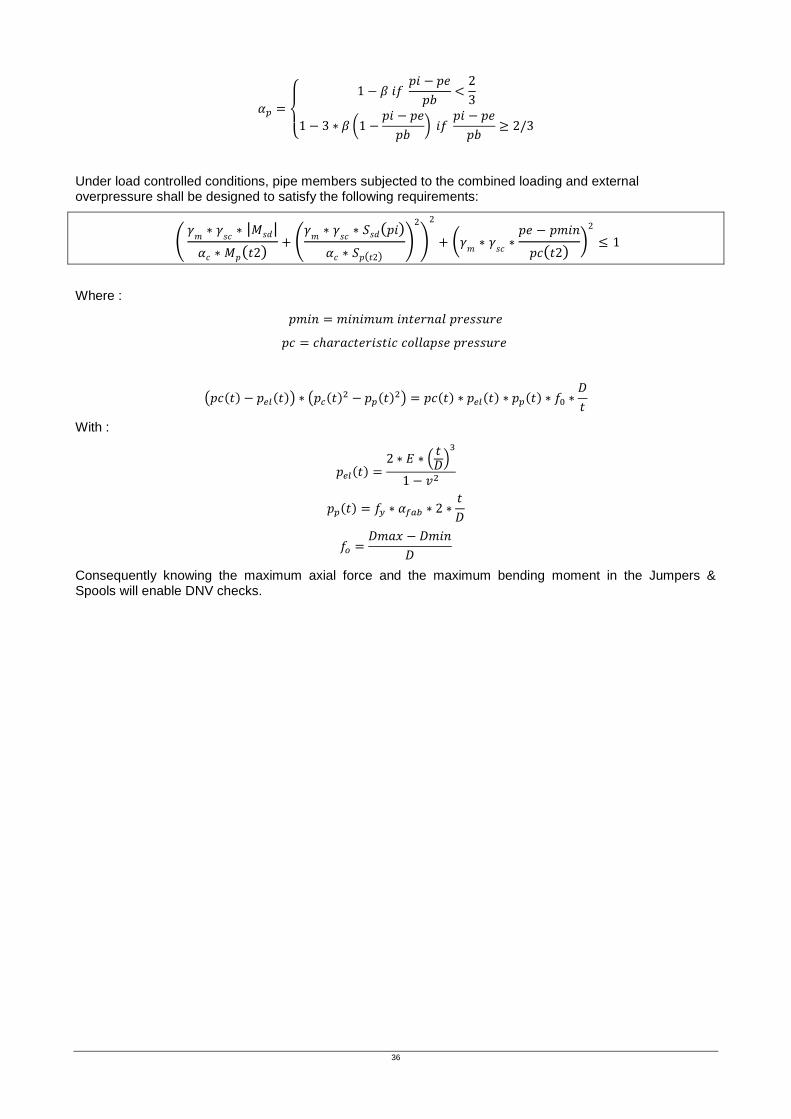
Under load controlled conditions, pipe members subjected to the combined loading and external overpressure shall be designed to satisfy the following requirements:

Where :

With :

Consequently knowing the maximum axial force and the maximum bending moment in the Jumpers & Spools will enable DNV checks.

37

4. THESIS ACTIVITY DESCRIPTION: JUMPERS & SPOOLS FEA DESIGN SPREADSHEETS

4.1 AUTOPIPE & ABAQUS FEA NUMERICAL MODELS

Finite Element Analysis are used to compute the values of the internal forces and moments in the complete jumper. AUTOPIPE is a piping FEA software which includes characteristic functionalities for analysis in that field. Consequently the post-processing of the outputs data is performed automatically by the software to comply with the ASME code. However ABAQUS is a general FEA software thus manual post-processing of the outputs data will be necessary. AUTOPIPE will also require post-processing to comply with DNV standards. The following part will deal with the two FEA software used to model Jumpers and Spools. The input files and the theoretical concepts will be detailed.

4.1.1 AUTOPIPE

Bentley AutoPIPE v8 Plus Ref.[8]. is a PC-based pipe stress analysis program by Bentley Systems which uses a finite element method to calculate the piping response to self-weight, pipe contents and external loads for subsea applications, taking into account the piping stiffness. Boundary conditions are applied at the restrained nodes of the model. All the models created have the following common features:

The model consists of pipe elements for straight section and elbow elements for bends. AutoPIPE automatically calculate the flexibility and stress intensification factor based on ASME B31.8 piping code, for bends.

The connectors are modelled as pipe elements with the effective submerged net weight and conservative stiffness.

Buoyancy module is modelled as an uplift force with net buoyancy where as appropriate.

The ends of the model are anchored with the imposed displacements to simulate the tolerance / misalignment and/or pipeline expansion as appropriate.

The end cap effect is automatically computed by AutoPIPE.

Environmental loading due to current is determined using AUTOPIPE and applied in the most

onerous directions. The Morison equation

is used to model such actions.

Soil is modelled as contact elements with downward linear stiffness and lateral friction.

Figure 32. Autopipe view, Jumper under gravity load & middle buoyancy

The input file of AUTOPIPE are *.NTL file. Indeed it is possible to model structures on AUTOPIPE whether using the software module or redacting input files. The advantage of possible automatism favors the use of *.NTL files (See Attachment B for a typical NTL file) The model geometry is created by the introduction of straight and bend segments. The aim of this study is to model both 2D Jumpers and 3D Spools. Each extremity of segment will represent a node in the analysis. For the bend, the curvature radius should be computed.

38

The connectors at the extremities of the Jumpers will be modeled by rigid elements. The Hub length and the pup piece length of each jumper being different, it is necessary to define and parameterize the size of those extremities. All the jumpers shall be designed to accommodate the following tolerances and misalignments:

Metrology tolerance

Fabrication tolerance

Expansions

Settlement

Through those tolerances are not very probable to combine synchronously, testing all the combinations enable the piping engineer to evaluate the most conservative situation. Additionally the expansions and the settlements will be added to the imposed displacements. The angular & linear tolerances due to metrology and fabrication are listed below.

DX : Linear tolerance along (OX) + Expansion projected on (OX) DY : Linear tolerance along (OY) + Expansion projected on (OY) DZ : Linear tolerance along (OZ) + Settlement

RX : Angular tolerance (pitch) RY : Angular tolerance (yaw) RZ : Rotation around (OZ) axis (roll)

The displacements matrix will be generated automatically by the spreadsheet according to the load case considered.

The deformed shape of the structure is highlighting the gravity, the wave load and all the displacements. Opening the models developed via the coding *.NTL, Autopipe enables the user to check that the structure is correctly designed and the loads are well applied.

Figure 33. Autopipe view, Deformed shape jumper under gravity load

39

Figure 34. 3D Spool designed on Autopipe

Both vertical and horizontal Spools have been designed during the project. The Figure 34 shows a L shaped Spool that has been modelled with the fixed anchors at each extremities and the connector weight applied.

The software enables an easy post processing in compliance with ASME B31.8. Indeed it is possible to obtain directly the ratios of the hoop, longitudinal and combined stresses with the allowable stresses.

Figure 35. ASME Stress checks are performed by Autopipe

40

4.1.2 ABAQUS

The 3D finite pipe element used in the established model is a two node twelve degree of freedom PIPE31H element. The element uses linear interpolation and therefore has a lumped mass distribution. The hybrid formulation makes the element well suited for case with slender structures and contact problems, such as a pipe lying on the seabed.

. Figure 36. Two nodes twelve degrees of freedom 3D pipe element

The hybrid elements are provided in Abaqus/Standard for use in cases where it is numerically difficult to compute the axial and shear forces in the beam by the usual finite element displacement method. The problem in such case is that slight differences in nodal positions can cause very large force in some part of the model, which, in turn cause large motions in other directions. The hybrid elements overcome this difficulty by using a more general formulation in which the axial and transverse shear forces in the elements are included, along, with the node displacements and rotations, as primary variables. Although this formulation makes these elements more calculation intensive, they generally converge much faster when the pipe rotations are large and are more efficient overall in such cases. The PIPE31H element is available with a hollow thin-walled circular section and supports the possibility for the user to specify external and/or internal pressure. The element can also account for changes in the pipe section area due to high axial straining of the pipe.

Pipe elements (PIPE21, PIPE22, PIPE31, PIPE32 and their “hybrid” equivalents) allow for transverse shear deformation. (plane sections initially normal to beam’s axis do not always remain plane and normal to the beam axis. They can be used for thick as well as slender beams.

The element-based loads that will be applied on the model are :

GRAV, gravity loading in a specified direction (magnitude is input as acceleration)

PX, force per unit length in global X-axis (used for the Morison current actions along (OX))

PY, force per unit length in global Y-axis (used for the Morison current actions along (OY))

HPI, hydrostatic internal pressure (closed-end condition), varying linearly with the global Z-coordinate

HPE, hydrostatic external pressure (closed-end condition), varying linearly with the global Z-coordinate

The element outputs are :

S11 : Axial stress.

S22 : Hoop stress.

S12 : Shear stress caused by torsion.

SF1 : Axial force.

SF2 : Transverse shear force in the local 2-direction.

SF3 : Transverse shear force in the local 1-direction.

SM1 : Bending moment about the local 1-axis.

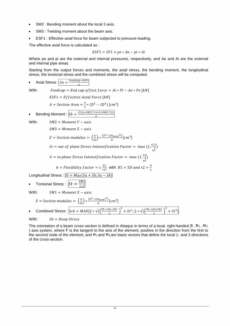
41

SM2 : Bending moment about the local 2-axis.

SM3 : Twisting moment about the beam axis.

ESF1 : Effective axial force for beam subjected to pressure loading.

The effective axial force is calculated as :

Where pe and pi are the external and internal pressures, respectively, and Ae and Ai are the external and internal pipe areas.

Starting from the output forces and moments, the axial stress, the bending moment, the longitudinal stress, the torsional stress and the combined stress will be computed.

Axial Stress :

With:

Bending Moment :

With:

with

Longitudinal Stress :

Torsional Stress :

With:

Combined Stress :

With:

The orientation of a beam cross-section is defined in Abaqus in terms of a local, right-handed ( , , ) axis system, where is the tangent to the axis of the element, positive in the direction from the first to the second node of the element, and and are basis vectors that define the local 1- and 2-directions of the cross-section.

42

Figure 37. Beam orientation

In Abaqus, a series of points is entered and these points are linked by straight line segments, each of which is integrated numerically along the axis of the section so that the section can be used together with non-linear material behavior. An independent thickness is associated with each of the segments making up the arbitrary section.

Pipe cross section will be used in our model. The outside radius and wall thickness of the cross section are entered. The beam considered being in space, 8 integration points (trapezoidal rule) are used. The output points will be the points 1,3,5 and 7 in the figure above.

It would also be possible to use thick pipe sections if more accurate stress values inside the wall thickness would be required. Then three points would be created radially in the thickness.

Figure 39. Default integration, beam in space, thin pipe section

Sensitivity analysis performed at Saipem have shown that element length of approximatively one Outside Diameter width insure convergence of the analysis for Jumpers and Spools. The spreadsheets developed have been made so to let the user free to choose the element length.

The *.INP file has been created taking into account the consideration above.(see Attachment 1 for a typical Abaqus file developed).

If more advanced analysis are required, usually in the bends, the use of thick beam section with brick or shell elements could be an option. Indeed the thickness of the pipe would then be more precisely described. Some convergence analysis on both type of 3D element have been carried.

Figure 38. Default integration, beam in space, thick pipe section

43

Figure 40. 3D bend Mesh with Shell Elements

Figure 41. 3D bend Mesh with Brick Elements

Preliminary analyses have shown that for thin pipes the results are very similar, see Figure 42. On the other hand, for thick pipes, the solid 3D Brick elements are in general conservative with respect to Shell elements, as shown in Figure 43, being the difference in the order of 6%. Consequently 3D Brick (BRICK) elements should be preferred in the design of precise pipeline bends.

Figure 42. Brick vs Shell Comparaison - Results for thin pipes

44

Figure 43. Brick vs Shell Comparaison - Results for thick pipes

The Abaqus *.ODB file enables us to verify that the Jumper model is correctly created. The checks conducted are:

The geometry of the pipeline.

The deformed shape under gravity load, wave load and imposed displacements.

The reaction load RF3 at the connector (cf calculation note below)

The rigidity of the connector

Figure 44. Jumper with an imposed displacement on ABAQUS

The gravity load case with the connector weights is used to check that the correct weight is applied on the structure. The reactions forces at both ends are extracted. Their values should be equal to the weight of the jumper with the connector loads.

Gravity case with connectors RF1 (N) RF3 (N)

Force at ends 1/2 7447 59287/59522

From RF3 value, we check that the weight is correctly applied :

45

With ; ;

The abaqus file developed is embedding the complete range of imposed displacements i.e. metrology and fabrication tolerances as well as the expansions. Each step is relating to one imposed displacement at the extremity. This processing way is valid as long as the imposed displacements are not excessively high and imply plasticity of the structure, because of residual deformations.

46

4.2 INPUT SPREADSHEET

The purpose of the input spreadsheet (FORM-SSA-SFD-FLOWS-054-E) is:

To generate jumpers models for both the FEA tools Abaqus and Autopipe.

To create the range of imposed displacements at the extremities and to apply those conditions to the structures.

To run the input files automatically in batch mode.

VBA code has been used to automatize the processing of the spreadsheet. At first the possibility of the spreadsheet only applied for the design of M-shaped plan jumpers on vertical support. Further developments will include 3D Jumpers and Spools lying on the seabed.

The input spreadsheet enables to design in the same action several Jumpers with 6 load cases each (As Landed, Hydrotest, Leak Test, Operating, Design and Shut Down). Buoyancy modules can be applied on every location on the structure. Both the Abaqus and Autopipe models are created by the spreadsheet.

Standard quality requirements of the Flowline Department of Saipem have been respected. The spreadsheet is composed of 7 worksheets:

COVER PAGE, REVISION HISTORY, INPUT, DISPL, INP, NTL, RESULTS.

47

1) “COVER PAGE” WORKSHEET

/

This document is t he p ropert y o f t he C ON TR A C TOR who wil l saf eguard it s r ight s accord ing t o t he civil and penal p rovisions o f t he law.

dd/mm/yyyyLOCATION

Project TitleLocation

N/AStatus Page

N/ADoc. Title Doc. Class

ABAQUS AND AUTOPIPE DESIGN TOOL M-SHAPED JUMPER N/A

CLIENT

CLIENT PROJECT TITLE

CLIENT

Doc. N°

CONTRACTOR

Job / Doc. N°N/A

Date

N/A

Rev.WBS

31N/A

ABAQUS AND AUTOPIPE DESIGN TOOL M-SHAPED JUMPER

CHECKED APPROVED

dd/mm/yyyy bybyN/A

PREPARED

Issued for interdiscipline check

REV. DATE DESCRIPTION

by

48

2) “REVISION HISTORY” WORKSHEET

/

REVISION HISTORY

List of HOLDs

This document is t he p ropert y o f t he C ON TR A C TOR who wil l saf eguard it s r ight s accord ing t o t he civil and penal p rovisions o f t he law.

PageHOLD DescriptionN°

LOCATION

N/A

N/A dd/mm/yyyyN/A

N/A

StatusDoc. Class

Rev. Status Date

ABAQUS AND AUTOPIPE DESIGN TOOL M-SHAPED JUMPER

Doc. Title

CLIENT Project Title

N/A

Location Rev.

CLIENT

Doc. N°

CONTRACTOR

Job / Doc. N°N/A

DateWBS

CLIENT PROJECT TITLE

1

2

Page

Update / Amendment Details

32

3

4

5

6

7

8

9

10

49

3) “INPUT” WORKSHEET

1.0 REFERENCES & FILES

1.1 Reference codes

[1]

[2]

1.2 Projet reference

[3]

[4]

1.3 Files names

1.3.1 Base folder ?

1.3.2 Input file Spreadsheet FORM-SSA-SFD-FLOWS-054-E

1.3.3 Post processing AUTOPIPE Spreadsheet FORM-SSA-SFD-FLOWS-055-E

1.3.4 Post processing ABAQUS Spreadsheet FORM-SSA-SFD-FLOWS-056-E

1.3.5 Autopipe folder C:\users-apps\Bentley\AutoPIPE V8i SELECTseries3

1.3.6 Abaqus folder C:\users-apps\ABAQUS

2.0 INPUTS

2.1 Identification

2.1.1 Is the jumper to be analyzed ? (YES=1) / (NO=0) Units Check 1

2.1.2 Jumper Tag Jumper_tag Ref : WIJ-04

2.1.3 Configuration Config Ref : NOM

2.1.4 End 1 end1 Ref : WFTA-04S

2.1.5 End 2 end2 Ref : WFTA-01

2.2 Pipe Dimensions

2.2.1 OD OD Ref : mm [_] 323.9

2.2.2 WT WT Ref : mm [_] 20.6

2.2.3 Corrosion allowance corr_all Ref : mm [_] 0

2.2.4 WT tolerance wt_tol Ref : mm [_] 4.532

2.3 Coating / Insulation

2.3.1 Coating Thickness coat_wt Ref : mm [_] 0

2.3.2 Density of coating coat_density kg/m3 [_] 671

2.4 Cladding

2.4.1 Clad Thickness clad_wt Ref : mm [_] 0

2.4.2 Density of cladding clad_density Ref : kg/m3 [_] 8840

2.5 Seawater data

2.5.1 Seawater density sea_desnity Ref : kg/m3 [_] 1025

2.5.2 Water depth WD Ref : m [_] 1098

2.6 Jumper Dimensions

2.6.1 L L Ref : mm [_] 25800

2.6.2 H H Ref : mm [_] 8500

2.6.3 Hc1 Hc_end1 Ref : mm [_] 7554

2.6.4 Ll1 Lloop_end1 Ref : mm [_] 2916

2.6.5 Hc2 Hc_end2 Ref : mm [_] 7727

2.6.6 Ll2 Lloop_end2 Ref : mm [_] 2916

2.7 Bend properties

2.7.1 Bend radius (x times D) bend_rad Ref : [_] 3

2.7.2 Radius considered Ref : [_] ID

2.7.3 Bend thining Ref : % [_] 16

2.8 Connectors

2.8.1 Connector submerged weight -end1 weight_end1 Ref : kg [_] 1085

2.8.2 Connector submerged weight -end2 weight_end2 Ref : kg [_] 1085

2.8.3 Hub length hub_length Ref : mm [_] 297

2.8.4 Pup piece length pup_length Ref : mm [_] 10

2.9 Hydrodynamic

2.9.1 Drag coefficient drag Ref : [_] 1.2

2.9.2 Lift coefficient lift Ref : [_] 0

2.10 Metrology & Fabrication

2.10.1 Linear tolerance -shared by each end linr_tol Ref : mm [_] 62.5

2.10.2 Angular tolerance -shared by each end anglr_tol Ref : degree (°) [_] 1

2.11 Layout angles

2.11.1 Jumper angle end1 jump_angl1 Ref : degree (°) [_] 50.9

2.11.2 Jumper angle end2 jump_angl2 Ref : degree (°) [_] -42.5

2.12 Buoyancy Module 1

2.12.1 Node number on ABAQUS nd_abaqus Ref : [_] 1

2.12.2 Node number on AUTOPIPE nd_autopipe Ref : [_] 33

2.12.3 Force value Fbuoy Ref : kN [_] 0

2.13 Buoyancy Module 2

2.13.1 Node number on ABAQUS nd_abaqus Ref : [_] 1

2.13.2 Node number on AUTOPIPE nd_autopipe Ref : [_] 0

2.13.3 Force value Fbuoy Ref : kN [_] 0

2.14 Buoyancy Module 3

2.14.1 Node number on ABAQUS nd_abaqus Ref : [_] 1

2.14.2 Node number on AUTOPIPE nd_autopipe Ref : [_] 0

2.14.3 Force value Fbuoy Ref : kN [_] 0

2.15 Load cases

2.15.1 AsLANDED to check or not : (YES=1) / (NO=0) 1

2.15.1.1 Content density cont_density Ref : kg/m3 [_] 1025

2.15.1.2 Pressure internal Pi Ref : bar [_] 109.8

2.15.1.3 Pressure external Pe Ref : bar [_] 109.8

2.15.1.4 Temperature internal Ti Ref : °C [_] 4

2.15.1.5 Temperature external Te Ref : °C [_] 4

2.15.1.6 Expansion end1 Exp_1 Ref : mm [_] 0

2.15.1.7 Expansion end2 Exp_2 Ref : mm [_] 0

2.15.1.8 Current angle with jumper planecurrent_angle Ref : degree (°) [_] 90

2.15.1.9 Current velocity current_velocityRef : m/s [_] 0.18

2.15.1.10 Pipeline Submerged Weight (Operating)sw_o Ref : kN/m [_] 1.31

2.15.1.11 Settlement End 1 stl_end1 Ref : mm [_] -44

2.15.1.12 Settlement End 2 stl_end2 Ref : mm [_] 0

2.15.2 HYDROTEST to check or not : (YES=1) / (NO=0) 0

2.15.2.1 Content density cont_density Ref : kg/m3 [_]

2.15.2.2 Pressure internal Pi Ref : bar [_]

2.15.2.3 Pressure external Pe Ref : bar [_]

2.15.2.4 Temperature internal Ti Ref : °C [_]

2.15.2.5 Temperature external Te Ref : °C [_]

2.15.2.6 Expansion end1 Exp_1 Ref : mm [_]

2.15.2.7 Expansion end2 Exp_2 Ref : mm [_]

2.15.2.8 Current angle with jumper planecurrent_angle Ref : degree (°) [_]

2.15.2.9 Current velocity current_velocityRef : m/s [_]

2.15.2.10 Pipeline Submerged Weight (Operating)sw_o Ref : kN/m [_]

2.15.2.11 Settlement End 1 stl_end1 Ref : mm [_]

2.15.2.12 Settlement End 2 stl_end2 Ref : mm [_]

2.15.3 LEAK_TEST to check or not : (YES=1) / (NO=0) 0

2.15.3.1 Content density cont_density Ref : kg/m3 [_]

2.15.3.2 Pressure internal Pi Ref : bar [_]

2.15.3.3 Pressure external Pe Ref : bar [_]

2.15.3.4 Temperature internal Ti Ref : °C [_]

2.15.3.5 Temperature external Te Ref : °C [_]

2.15.3.6 Expansion end1 Exp_1 Ref : mm [_]

2.15.3.7 Expansion end2 Exp_2 Ref : mm [_]

2.15.3.8 Current angle with jumper planecurrent_angle Ref : degree (°) [_]

2.15.3.9 Current velocity current_velocityRef : m/s [_]

2.15.3.10 Pipeline Submerged Weight (Operating)sw_o Ref : kN/m [_]

2.15.3.11 Settlement End 1 stl_end1 Ref : mm [_]

2.15.3.12 Settlement End 2 stl_end2 Ref : mm [_]

2.15.4 DESIGN to check or not : (YES=1) / (NO=0) 0

2.15.4.1 Content density cont_density Ref : kg/m3 [_]

2.15.4.2 Pressure internal Pi Ref : bar [_]

2.15.4.3 Pressure external Pe Ref : bar [_]

2.15.4.4 Temperature internal Ti Ref : °C [_]

2.15.4.5 Temperature external Te Ref : °C [_]

2.15.4.6 Expansion end1 Exp_1 Ref : mm [_]

2.15.4.7 Expansion end2 Exp_2 Ref : mm [_]

2.15.4.8 Current angle with jumper planecurrent_angle Ref : degree (°) [_]

2.15.4.9 Current velocity current_velocityRef : m/s [_]

2.15.4.10 Pipeline Submerged Weight (Operating)sw_o Ref : kN/m [_]

2.15.4.11 Settlement End 1 stl_end1 Ref : mm [_]

2.15.4.12 Settlement End 2 stl_end2 Ref : mm [_]

2.15.5 OPERATING to check or not : (YES=1) / (NO=0) 1

2.15.5.1 Content density cont_density Ref : kg/m3 [_] 1025

2.15.5.2 Pressure internal Pi Ref : bar [_] 276

2.15.5.3 Pressure external Pe Ref : bar [_] 109.8

2.15.5.4 Temperature internal Ti Ref : °C [_] 26.5

2.15.5.5 Temperature external Te Ref : °C [_] 4

2.15.5.6 Expansion end1 Exp_1 Ref : mm [_] 379

2.15.5.7 Expansion end2 Exp_2 Ref : mm [_] 400

2.15.5.8 Current angle with jumper planecurrent_angle Ref : degree (°) [_] 90

2.15.5.9 Current velocity current_velocityRef : m/s [_] 0.18

2.15.5.10 Pipeline Submerged Weight (Operating)sw_o Ref : kN/m [_] 1.31

2.15.5.11 Settlement End 1 stl_end1 Ref : mm [_] -106

2.15.5.12 Settlement End 2 stl_end2 Ref : mm [_] -100

2.15.6 SHUT_DOWN to check or not : (YES=1) / (NO=0) 0

2.15.6.1 Content density cont_density Ref : kg/m3 [_]

2.15.6.2 Pressure internal Pi Ref : bar [_]

2.15.6.3 Pressure external Pe Ref : bar [_]

2.15.6.4 Temperature internal Ti Ref : °C [_]

2.15.6.5 Temperature external Te Ref : °C [_]

2.15.6.6 Expansion end1 Exp_1 Ref : mm [_]

2.15.6.7 Expansion end2 Exp_2 Ref : mm [_]

2.15.6.8 Current angle with jumper planecurrent_angle Ref : degree (°) [_]

2.15.6.9 Current velocity current_velocityRef : m/s [_]

2.15.6.10 Pipeline Submerged Weight (Operating)sw_o Ref : kN/m [_]

2.15.6.11 Settlement End 1 stl_end1 Ref : mm [_]

2.15.6.12 Settlement End 2 stl_end2 Ref : mm [_]

3.0 CALCULATIONS

3.1 RUN ABAQUS

3.1.1 Creation of inp file 0

3.1.2 Abaqus running 0

3.1.3 Post processing Abaqus 0

3.2 RUN AUTOPIPE

3.2.1 Creation of ntl file 0

3.2.2 Autopipe running 0

3.2.3 Post processing Autopipe 0

Create INP Files and Run ABAQUS

Create NTL Files and Run AUTOPIPE

Hc1

Hc2

Ll1 Ll2

H

L

RESET

RESET

Post Processing ABAQUS

Post Processing AUTOPIPE

DELETE ALL

ADD A JUMPER DELETE A JUMPER

13

11

2126

36

41

51 6676

81

9196

106

111114116

nodes ABAQUS

50

A better view of the spreadsheet is given here below :

Figure 45. Input Spreadsheet

Each column of the spreadsheet can be used for a jumper. The input variables needed to be entered are:

2.0 INPUTS subdivisions Descriptions

IDENTIFICATION Allows user to provide names for : Jumper Tag, Configuration, End 1, End 2.

PIPE DIMENSIONS OD, WT, Corrosion Allowance (CA),WT tolerance

COATING / INSULATION Coating Thickness, Density coating

CLADDING Cladding Thickness, Density cladding

2.0 INPUTS

2.1 Identification

2.1.1 Is the jumper to be analyzed ? (YES=1) / (NO=0) Units Check 1

2.1.2 Jumper Tag Jumper_tag Ref : WIJ-04

2.1.3 Configuration Config Ref : NOM

2.1.4 End 1 end1 Ref : WFTA-04S

2.1.5 End 2 end2 Ref : WFTA-01

2.2 Pipe Dimensions

2.2.1 OD OD Ref : mm [_] 323.9

2.2.2 WT WT Ref : mm [_] 20.6

2.2.3 Corrosion allowance corr_all Ref : mm [_] 0

2.2.4 WT tolerance wt_tol Ref : mm [_] 4.532

2.3 Coating / Insulation

2.3.1 Coating Thickness coat_wt Ref : mm [_] 0

2.3.2 Density of coating coat_density kg/m3 [_] 671

2.4 Cladding

2.4.1 Clad Thickness clad_wt Ref : mm [_] 0

2.4.2 Density of cladding clad_density Ref : kg/m3 [_] 8840

2.5 Seawater data

2.5.1 Seawater density sea_desnity Ref : kg/m3 [_] 1025

2.5.2 Water depth WD Ref : m [_] 1098

2.6 Jumper Dimensions

2.6.1 L L Ref : mm [_] 25800

2.6.2 H H Ref : mm [_] 8500

2.6.3 Hc1 Hc_end1 Ref : mm [_] 7554

2.6.4 Ll1 Lloop_end1 Ref : mm [_] 2916

2.6.5 Hc2 Hc_end2 Ref : mm [_] 7727

2.6.6 Ll2 Lloop_end2 Ref : mm [_] 2916

2.7 Bend properties

2.7.1 Bend radius (x times D) bend_rad Ref : [_] 3

2.7.2 Radius considered Ref : [_] ID

2.7.3 Bend thining Ref : % [_] 16

2.8 Connectors

2.8.1 Connector submerged weight -end1 weight_end1 Ref : kg [_] 1085

2.8.2 Connector submerged weight -end2 weight_end2 Ref : kg [_] 1085

2.8.3 Hub length hub_length Ref : mm [_] 6000

2.8.4 Pup piece length pup_length Ref : mm [_] 20

2.9 Hydrodynamic

2.9.1 Drag coefficient drag Ref : [_] 1.2

2.9.2 Lift coefficient lift Ref : [_] 0

2.10 Metrology & Fabrication

2.10.1 Linear tolerance -shared by each end linr_tol Ref : mm [_] 62.5

2.10.2 Angular tolerance -shared by each end anglr_tol Ref : degree (°) [_] 1

2.11 Layout angles

2.11.1 Jumper angle end1 jump_angl1 Ref : degree (°) [_] 50.9

2.11.2 Jumper angle end2 jump_angl2 Ref : degree (°) [_] -42.5

2.12 Buoyancy Module 1

2.12.1 Node number on ABAQUS nd_abaqus Ref : [_] 0

2.12.2 Node number on AUTOPIPE nd_autopipe Ref : [_] 33

2.12.3 Force value Fbuoy Ref : kN [_] 9

2.13 Buoyancy Module 2

2.13.1 Node number on ABAQUS nd_abaqus Ref : [_] 0

2.13.2 Node number on AUTOPIPE nd_autopipe Ref : [_] 0

2.13.3 Force value Fbuoy Ref : kN [_] 0

2.14 Buoyancy Module 3

2.14.1 Node number on ABAQUS nd_abaqus Ref : [_] 0

2.14.2 Node number on AUTOPIPE nd_autopipe Ref : [_] 0

2.14.3 Force value Fbuoy Ref : kN [_] 0

2.15 Load cases

2.15.1 AsLANDED to check or not : (YES=1) / (NO=0) 1

2.15.1.1 Content density cont_density Ref : kg/m3 [_] 1025

2.15.1.2 Pressure internal Pi Ref : bar [_] 109.8

2.15.1.3 Pressure external Pe Ref : bar [_] 109.8

2.15.1.4 Temperature internal Ti Ref : °C [_] 4

2.15.1.5 Temperature external Te Ref : °C [_] 4

2.15.1.6 Expansion end1 Exp_1 Ref : mm [_] 0

2.15.1.7 Expansion end2 Exp_2 Ref : mm [_] 0

2.15.1.8 Current angle with jumper planecurrent_angle Ref : degree (°) [_] 90

2.15.1.9 Current velocity current_velocityRef : m/s [_] 0.18

2.15.1.10 Pipeline Submerged Weight (Operating)sw_o Ref : kN/m [_] 1.31

2.15.1.11 Settlement End 1 stl_end1 Ref : mm [_] -44

2.15.1.12 Settlement End 2 stl_end2 Ref : mm [_] 0

51

2.0 INPUTS subdivisions Descriptions

SEA WATER DATA Seawater density, Water depth

JUMPER DIMENSIONS L, H, HC1, Ll1, HC2, Ll2 (see the Figure 45)

BEND PROPERTIES Bend radius (number of times OD or ID), Bend thinning in %

CONNECTORS Connectors Submerged weights at both extremities, Hub length, Pup piece lengths

HYDRODYNAMIC Drag coefficient, Lift coefficient

METROLOGY & FABRICATION Linear tolerances, Angular tolerances

LAYOUT ANGLES Line angle with jumper at end 1, Line angle with jumper at end 2 (used to calculate displacement caused by flowline in jumper coordinate system).

BUOYANCY MODULES Node number, Vertical up lift force

LOAD CASES Content density, PI, PE, TI, TE, Expansions, Current velocity, Current angle, Pipeline Submerged Weight, Settlement at both the extremities

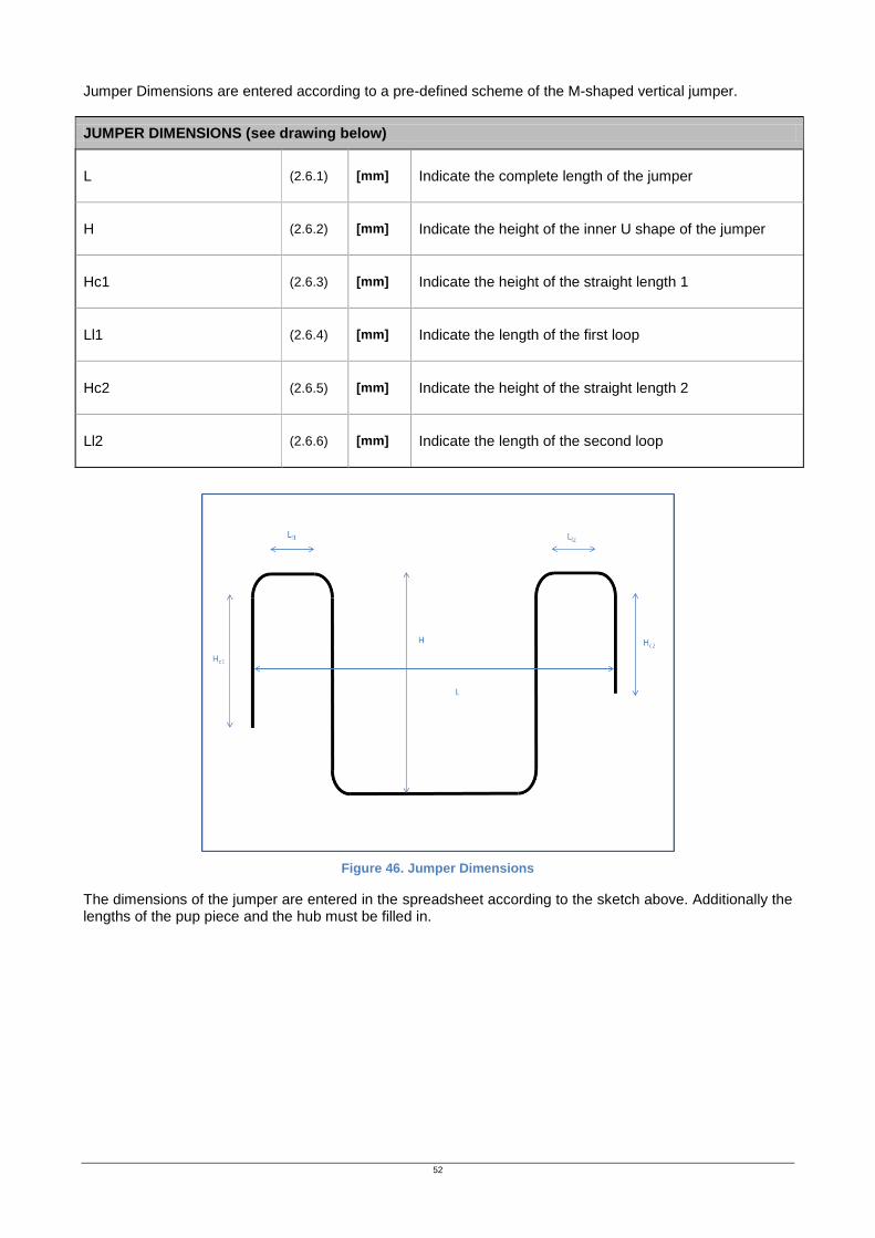
52

Jumper Dimensions are entered according to a pre-defined scheme of the M-shaped vertical jumper.

JUMPER DIMENSIONS (see drawing below)

L (2.6.1) [mm] Indicate the complete length of the jumper

H (2.6.2) [mm] Indicate the height of the inner U shape of the jumper

Hc1 (2.6.3) [mm] Indicate the height of the straight length 1

Ll1 (2.6.4) [mm] Indicate the length of the first loop

Hc2 (2.6.5) [mm] Indicate the height of the straight length 2

Ll2 (2.6.6) [mm] Indicate the length of the second loop

Figure 46. Jumper Dimensions

The dimensions of the jumper are entered in the spreadsheet according to the sketch above. Additionally the lengths of the pup piece and the hub must be filled in.

53

4) “INP” WORKSHEET

This excel worksheet is responsible of the generation of the Abaqus *.INP file starting from the input variables. Nodes coordinates, Pressure and Temperature conditions as well as Load Cases configurations are created by this worksheet using excel functions.

Folder

Jumper Tag

Configuration NOMINAL ***********************************************************************

OD (mm) 219.1 *HEADING

WT (mm) 20.6 0.0

Corrosion allowance (mm) 3 ***********************************************************************

WT tolerance (mm) 0 ****------------------------------------------------****

Coating WT (mm) 0 **** PIPE NODES ****

Density (kg/m3) 0 ****------------------------------------------------****

Clad WT (mm) 0 **

Density (kg/m3) 0 *RESTART , WRITE , OVERLAY

Seawater density (t/m3) 1027 *NODE , NSET=NODMOD

Water Depth (m) 1148 1,0,0,0

L (mm) 26439 3,0,0,0.297

H (mm) 8000 6,0,0,0.307

He1 (mm) 6090 11,0,0,5.3015

Ll1 (mm) 3192 21,1.0955,0,6.397

He2 (mm) 5666 26,2.0965,0,6.397

Ll2 (mm) 3192 36,3.192,0,5.3015

Bend radius (x times D) 5 41,3.192,0,-0.5075

Diamter considered OD 51,4.2875,0,-1.603

Connectors Connector weight - end1 (kg) 3786 66,22.1515,0,-1.603

Connector weight - end2 (kg) 3786 76,23.247,0,-0.5075

Hydrodynamic Drag coefficient 1.2 81,23.247,0,5.3015

Lift coefficient 0 91,24.3425,0,6.397

Pressure Pint (bar) 473 96,25.3435,0,6.397

Pext (bar) 115.3 106,26.439,0,5.3015

Temperature Tint (°C) 4 111,26.439,0,0.731

Text (°C) 4 114,26.439,0,0.721

Current Current angle with jumper plane (°) 90 116,26.439,0,0.424

Current velocity (m/s) 0.4 100001,1.0955,0,5.3015

Contents Content density (t/m3) 1027 100002,2.0965,0,5.3015

Torsion ? VRAI 100003,4.2875,0,-0.5075

100004,22.1515,0,-0.5075

Length_pup (mm) 10 100005,24.3425,0,5.3015

Length_hub (mm) 297 100006,25.3435,0,5.3015

Bend radius (m) 1.0955 ****************************************************** Jumper Straight Lines

Length1 (m) 4.9945 *NGEN,NSET=NODMOD

Length2 (m) 1.001 1,3,1

Length3 (m) 5.809 3,6,1

Length4 (m) 17.864 6,11,1

Length5 (m) 5.809 21,26,1

Length6 (m) 1.001 36,41,1

Length7 (m) 4.5705 51,66,1 X Y Z

Length_hub_half (m) 148.5 76,81,1

ID (m) 0.1779 91,96,1 n_ini1 1 0.000 0.000 0.000

R (m) 0.10955 106,111,1 n_ini2 3 0.000 0.000 0.297

WT (m) 0.0206 111,114,1 n_ini3 6 0.000 0.000 0.307

114,116,1 n_ini4 11 0.000 0.000 5.302

Start line 3 ************************************************ Elements pipe at straight lines n_ini5 21 1.096 0.000 6.397

End line 302 *ELEMENT,TYPE=PIPE31H,ELSET=EL_PIPE_SKETCH_HUB_LEFT n_ini6 26 2.097 0.000 6.397

1,1,2 n_ini7 36 3.192 0.000 5.302

F_waveX (kN/m) 1.32325E-18 *ELGEN,ELSET=EL_PIPE_SKETCH_HUB_LEFT n_ini8 41 3.192 0.000 -0.507

F_waveY (kN/m) 0.021601507 1,2,1,1,1 n_ini9 51 4.288 0.000 -1.603

** n_ini10 66 22.152 0.000 -1.603

*ELEMENT,TYPE=PIPE31H,ELSET=EL_PIPE_SKETCH_PUP_LEFT n_ini11 76 23.247 0.000 -0.507

3,3,4 n_ini12 81 23.247 0.000 5.302

E (kPa) 2.04E+08 *ELGEN,ELSET=EL_PIPE_SKETCH_PUP_LEFT n_ini13 91 24.343 0.000 6.397

Nu 0.3 3,3,1,1,1 n_ini14 96 25.344 0.000 6.397

K (°C-1) 0.0000175 ** n_ini15 106 26.439 0.000 5.302

steel_density (t/m3) 7.83 *ELEMENT,TYPE=PIPE31H,ELSET=EL_PIPE_SKETCH_VERT_UP n_ini16 111 26.439 0.000 0.731

SMYS (kPa) 450000 6,6,7 n_ini17 114 26.439 0.000 0.721

SMTS (kPa) 535000 *ELGEN,ELSET=EL_PIPE_SKETCH_VERT_UP n_fin 116 26.439 0.000 0.424

6,5,1,1,1 n_bend1 100001 1.096 0.000 5.302

** n_bend2 100002 2.097 0.000 5.302

Temp0 (°C) 4 *ELEMENT,TYPE=PIPE31H,ELSET=EL_PIPE_SKETCH_HORIZ n_bend3 100003 4.288 0.000 -0.507

Pe_leaktest (kPa) 47300 21,21,22 n_bend4 100004 22.152 0.000 -0.507

Pi_leaktest (kPa) 11530 *ELGEN,ELSET=EL_PIPE_SKETCH_HORIZ n_bend5 100005 24.343 0.000 5.302

Temp_leaktest (°C) 4 21,5,1,1,1 n_bend6 100006 25.344 0.000 5.302

**

*ELEMENT,TYPE=PIPE31H,ELSET=EL_PIPE_SKETCH_VERT_DOWN

g (m/s2) 9.81 36,36,37

subW_o1 (kN/m) 0.858 *ELGEN,ELSET=EL_PIPE_SKETCH_VERT_DOWN

conn_wght1 (kN) 37.14066 36,5,1,1,1

conn_wght2 (kN) 37.14066 ** 1 3 1 1 2 11 21 1 100001 11 11 12

*ELEMENT,TYPE=PIPE31H,ELSET=EL_PIPE_SKETCH_HORIZ 3 6 1 2 26 36 1 100002 11 10

Load Case Leak_test 51,51,52 6 11 3 3 4 41 51 1 100003 26 26 27

Load cases Number (step) 64 *ELGEN,ELSET=EL_PIPE_SKETCH_HORIZ 21 26 3 3 66 76 1 100004 26 10

51,15,1,1,1 36 41 6 6 7 81 91 1 100005 41 41 42

** 51 66 6 5 96 106 1 100006 41 10

start_line2 302 *ELEMENT,TYPE=PIPE31H,ELSET=EL_PIPE_SKETCH_VERT_UP 76 81 21 21 22 66 66 67

end_line2 1893 76,76,77 91 96 21 5 66 10

*ELGEN,ELSET=EL_PIPE_SKETCH_VERT_UP 106 111 36 36 37 81 81 82

76,5,1,1,1 111 114 36 5 81 10

** 114 116 51 51 52 96 96 97

Node 1 22 *ELEMENT,TYPE=PIPE31H,ELSET=EL_PIPE_SKETCH_HORIZ 51 15 96 10

Force 1 (kN) 6.5 91,91,92 76 76 77

Node 2 23 *ELGEN,ELSET=EL_PIPE_SKETCH_HORIZ 76 5 NODE SETS

Force 2 (kN) 5.6 91,5,1,1,1 91 91 92 1

Node 3 56 ** 91 5 116

Force 3 (kN) 8.1 *ELEMENT,TYPE=PIPE31H,ELSET=EL_PIPE_SKETCH_VERT_DOWN 106 106 ## 6

106,106,107 106 5 111

*ELGEN,ELSET=EL_PIPE_SKETCH_VERT_DOWN 111 111 ## 2

106,5,1,1,1 111 3 115

** 114 114 ##

*ELEMENT,TYPE=PIPE31H,ELSET=EL_PIPE_SKETCH_PUP_RIGHT 114 2

111,111,112

*ELGEN,ELSET=EL_PIPE_SKETCH_PUP_RIGHT

111,3,1,1,1

**

*ELEMENT,TYPE=PIPE31H,ELSET=EL_PIPE_SKETCH_HUB_RIGHT

114,114,115

*ELGEN,ELSET=EL_PIPE_SKETCH_HUB_RIGHT

114,2,1,1,1

**************************************************************** Jumper Bends

*NGEN,LINE=C,NSET=NODMOD

11,21,1,100001

26,36,1,100002

41,51,1,100003

66,76,1,100004

81,91,1,100005

96,106,1,100006

***************************************************** Elements Pipe at Bends

*ELEMENT,TYPE=PIPE31H,ELSET=EL_PIPE_SKETCH_BEND_CONCAVE_UP

INC1 500 11,11,12

min_inc1 1.00E-10 *ELGEN,ELSET=EL_PIPE_SKETCH_BEND_CONCAVE_UP

min_inc2 1.00E-10 11,10,1,1,1

ini_inc1 0.1 *ELEMENT,TYPE=PIPE31H,ELSET=EL_PIPE_SKETCH_BEND_CONCAVE_DOWN

ini_inc2 0.2 26,26,27

max_inc1 1 *ELGEN,ELSET=EL_PIPE_SKETCH_BEND_CONCAVE_DOWN

max_inc2 0.1 26,10,1,1,1

*ELEMENT,TYPE=PIPE31H,ELSET=EL_PIPE_SKETCH_BEND_CONVEXE_DOWN

41,41,42

*ELGEN,ELSET=EL_PIPE_SKETCH_BEND_CONVEXE_DOWN

41,10,1,1,1

x0 0 *ELEMENT,TYPE=PIPE31H,ELSET=EL_PIPE_SKETCH_BEND_CONVEXE_UP

z0 0 66,66,67

n_ini 1 *ELGEN,ELSET=EL_PIPE_SKETCH_BEND_CONVEXE_UP

n_ele1 5 66,10,1,1,1

n_ele2 5 *ELEMENT,TYPE=PIPE31H,ELSET=EL_PIPE_SKETCH_BEND_CONCAVE_UP

n_ele3 5 81,81,82

n_ele4 15 *ELGEN,ELSET=EL_PIPE_SKETCH_BEND_CONCAVE_UP

n_ele5 5 81,10,1,1,1

n_ele6 5 *ELEMENT,TYPE=PIPE31H,ELSET=EL_PIPE_SKETCH_BEND_CONCAVE_DOWN

n_ele7 5 96,96,97

n_elebend 10 *ELGEN,ELSET=EL_PIPE_SKETCH_BEND_CONCAVE_DOWN

n_elehub 2 96,10,1,1,1

n_elepup 3 ****------------------------------------------------****

n_bend1 100001 **** NODE SETS ****

n_bend2 100002 ****------------------------------------------------****

n_bend3 100003 *NSET,NSET=LEFTEND

n_bend4 100004 1

n_bend5 100005 *NSET,NSET=RIGHTEND

n_bend6 100006 116

n_conn1 5002 *NSET,NSET=LEFTCON

n_conn2 5115 2

*NSET,NSET=RIGHTCON

115

****------------------------------------------------****

**** PIPE SECTION ****

****------------------------------------------------****

*BEAM SECTION,SECTION=PIPE,ELSET=EL_PIPE_SKETCH_HUB_LEFT,MATERIAL=Connector_steel

0.10955,0.0206

-1,0,0

32

*BEAM SECTION,SECTION=PIPE,ELSET=EL_PIPE_SKETCH_PUP_LEFT,MATERIAL=DNV450

0.10955,0.0206

-1,0,0

32

*BEAM SECTION,SECTION=PIPE,ELSET=EL_PIPE_SKETCH_HUB_RIGHT,MATERIAL=Connector_steel

0.10955,0.0206

1,0,0

32

*BEAM SECTION,SECTION=PIPE,ELSET=EL_PIPE_SKETCH_PUP_RIGHT,MATERIAL=DNV450

0.10955,0.0206

1,0,0

32

*BEAM SECTION,SECTION=PIPE,ELSET=EL_PIPE_SKETCH_HORIZ,MATERIAL=DNV450

0.10955,0.0206

0,0,-1

32

*BEAM SECTION,SECTION=PIPE,ELSET=EL_PIPE_SKETCH_VERT_UP,MATERIAL=DNV450

0.10955,0.0206

-1,0,0

32

*BEAM SECTION,SECTION=PIPE,ELSET=EL_PIPE_SKETCH_VERT_DOWN,MATERIAL=DNV450

0.10955,0.0206

-1,0,0

32

*BEAM SECTION,SECTION=PIPE,ELSET=EL_PIPE_SKETCH_BEND_CONCAVE_UP,MATERIAL=DNV450

0.10955,0.0206

-1,0,0

32

*BEAM SECTION,SECTION=PIPE,ELSET=EL_PIPE_SKETCH_BEND_CONCAVE_DOWN,MATERIAL=DNV450

0.10955,0.0206

0,0,1

32

*BEAM SECTION,SECTION=PIPE,ELSET=EL_PIPE_SKETCH_BEND_CONVEXE_DOWN,MATERIAL=DNV450

0.10955,0.0206

1,0,0

32

*BEAM SECTION,SECTION=PIPE,ELSET=EL_PIPE_SKETCH_BEND_CONVEXE_UP,MATERIAL=DNV450

0.10955,0.0206

NGEN BEND ELGEN BEND

Step parameters

FE Mesh Elements

for each section

NODES

Wave Loads

Mechanical Prop.

Temperature &

Pressure

WeightsNGEN STRAIGHT ELGEN STRAIGHT

Buoyancies

Jumper dimensions

Z:\SFD\5_FLOWS\2_SEA_DES\4_ENGINEERS\Benoît\ZINIA\

Pipe Dimensions

Coating

Cladding

Water properties

Hc1

Hc2

Ll1 Ll2

H

L

1

36

11

2126

36

41

51 66

76

81

9196

106

111114

116

-3

-2

-1

0

1

2

3

4

5

6

7

-5 0 5 10 15 20 25 30

Bend centers

Jumper Geometry

LEFT END=1 RIGHT END=2

54

3) “NTL” WORKSHEET

This excel worksheet is responsible of the generation of the Autopipe *.NTL file starting from the input variables. Nodes coordinates, Pressure and Temperature conditions as well as Load Cases configurations are created by this worksheet using excel functions.

Folder

Jumper Tag AOKB-PLJW58304-01

Configuration NOMINAL JOB ED 1.7 09.04.01.05

OD (mm) 219.1 *

WT (mm) 20.6 HED BONGASW

Corrosion allowance (mm) 3.0 CTL O31.8 Z 100 006.00 SI SI AUTOPIPE AUTOB318

WT tolerance (mm) 0.0 * 2010 000.00

Coating WT (mm) 0.0 DESC ^n

Density (kg/m3) 0.0 * ^n ^n PRIN Y Y Y Y Y N N N N Y Y N N N Y N N N N N

Clad WT (mm) 0.0 * ^n ^n

Density (kg/m3) 0.0 * ^n ^n

Seawater density (kg/m3) 1027.0 * ^n

Water Depth (m) 1148.0 * ^n ^n ^e

L (mm) 26439.0 MINP N N Y Y Y Y Y Y N Y N N N N N N Y N N N N N Y N N N N

H (mm) 8000.0 BUOY 99000.000 1.027 1.000 #NOM? BUOY 99000.000 1.027 1.000

He1 (mm) 6090.0 PRIN Y Y Y Y Y

Ll1 (mm) 3192.0 ***

He2 (mm) 5666.0 SEG A00 0.000 0.000 0.000

Ll2 (mm) 3192.0 PIPE PIPE1 -219.100 20.600 3.000 0.000 PIPE PIPE1 -219.100 20.600 3.000 0.000

Bend radius (x times D) 5 *5LX-X65 322.675 .20427455 7833.028 .20427455

Diamter considered OD *O 000.0000 000.0000 1.0250 00.000 0000.0000 *O 000.0000 000.0000 1.0250 00.000 0000.0000

Connectors Connector weight - end1 (kg) 3786.0 * 1.0000 1.0000 .078567132 448.160 21 *O

Connector weight - end2 (kg) 3786.0 * 29 *O 000.0000

Hydrodynamic Drag coefficient 1.2 * 31 *O 000.0000

Lift coefficient 0.0 ANC F 000000 39 *O 000.0000 000.0000

Pressure Pint (bar) 340.0 DISP T1 0562.500 0000.000 -0044.000 0001.250 0001.250 0000.000 41 *O 000.0000 000.0000

Pext (bar) 0.0 DISP T2 0562.500 0000.000 -0044.000 0001.250 0001.250 0000.000 47 *O 000.0000 000.0000 1.0250

Temperature Tint (°C) 6.0 DISP T3 0562.500 0000.000 -0044.000 0001.250 0001.250 0000.000 51 *O 000.0000 000.0000 1.0250

Text (°C) 6.0 DISP T4 0562.500 0000.000 -0044.000 0001.250 0001.250 0000.000 57 *O 000.0000 000.0000 1.0250 00.000

Current Current angle with jumper plane (°) 90.0 DISP T5 0562.500 0000.000 -0044.000 0001.250 0001.250 0000.000 61 *O 000.0000 000.0000 1.0250 00.000

Current velocity (m/s) 0.4 DISP T6 0562.500 0000.000 -0044.000 0001.250 0001.250 0000.000 70 *O 000.0000 000.0000 1.0250 00.000 0000.0000

Contents Content density (kg/m3) 1025.0 DISP T7 0562.500 0000.000 -0044.000 0001.250 0001.250 0000.000

Torsion ? VRAI DISP T8 0562.500 0000.000 -0044.000 0001.250 0001.250 0000.000

DISP T9 0562.500 0000.000 -0044.000 0001.250 -0001.250 0000.000

DISP T10 0562.500 0000.000 -0044.000 0001.250 -0001.250 0000.000

DISP T11 0562.500 0000.000 -0044.000 0001.250 -0001.250 0000.000

DISP T12 0562.500 0000.000 -0044.000 0001.250 -0001.250 0000.000

DISP T13 0562.500 0000.000 -0044.000 0001.250 -0001.250 0000.000

Pup piece (mm) 10 DISP T14 0562.500 0000.000 -0044.000 0001.250 -0001.250 0000.000

Loop1 straight length (mm) 979.09 DISP T15 0562.500 0000.000 -0044.000 0001.250 -0001.250 0000.000

Loop2 straight length (mm) 979.09 DISP T16 0562.500 0000.000 -0044.000 0001.250 -0001.250 0000.000

Height straight length (mm) 5787.09 DISP T17 0562.500 0000.000 -0044.000 -0001.250 0001.250 0000.000

Middle straight length (mm) 17842.09 DISP T18 0562.500 0000.000 -0044.000 -0001.250 0001.250 0000.000

End 1 to conn. Straight (mm) 4983.5 DISP T19 0562.500 0000.000 -0044.000 -0001.250 0001.250 0000.000

End 2 to conn. Straight (mm) 4559.5 DISP T20 0562.500 0000.000 -0044.000 -0001.250 0001.250 0000.000

Conn (mm) 297 DISP T21 0562.500 0000.000 -0044.000 -0001.250 0001.250 0000.000 OPER A 00 1 6.000 034.000 A A 66

g (N/kg) 9.81 DISP T22 0562.500 0000.000 -0044.000 -0001.250 0001.250 0000.000 * A

Bend radius (mm) 1095.5 DISP T23 0562.500 0000.000 -0044.000 -0001.250 0001.250 0000.000 OPER A 00 2 6.000 034.000 A A 66

Other 1106.5 DISP T24 0562.500 0000.000 -0044.000 -0001.250 0001.250 0000.000 * A

Start line 3 DISP T25 0562.500 0000.000 -0044.000 -0001.250 -0001.250 0000.000 OPER A 00 3 6.000 034.000 A A 66

End line 433 DISP T26 0562.500 0000.000 -0044.000 -0001.250 -0001.250 0000.000 * A

DISP T27 0562.500 0000.000 -0044.000 -0001.250 -0001.250 0000.000 OPER A 00 4 6.000 034.000 A A 66

26439 DISP T28 0562.500 0000.000 -0044.000 -0001.250 -0001.250 0000.000 * A

DISP T29 0562.500 0000.000 -0044.000 -0001.250 -0001.250 0000.000 OPER A 00 5 6.000 034.000 A A 66

DISP T30 0562.500 0000.000 -0044.000 -0001.250 -0001.250 0000.000 * A

DISP T31 0562.500 0000.000 -0044.000 -0001.250 -0001.250 0000.000 OPER A 00 6 6.000 034.000 A A 66

Node 1 12 DISP T32 0562.500 0000.000 -0044.000 -0001.250 -0001.250 0000.000 * A

Force 1 (kN) 0 DISP T33 0437.500 0000.000 -0044.000 0001.250 0001.250 0000.000 OPER A 00 7 6.000 034.000 A A 66

Node 2 02 DISP T34 0437.500 0000.000 -0044.000 0001.250 0001.250 0000.000 * A

Force 2 (kN) 0 DISP T35 0437.500 0000.000 -0044.000 0001.250 0001.250 0000.000 OPER A 00 8 6.000 034.000 A A 66

Node 3 54 DISP T36 0437.500 0000.000 -0044.000 0001.250 0001.250 0000.000 * A

Force 3 (kN) 0 DISP T37 0437.500 0000.000 -0044.000 0001.250 0001.250 0000.000 OPER A 00 9 6.000 034.000 A A 66

DISP T38 0437.500 0000.000 -0044.000 0001.250 0001.250 0000.000 * A

DISP T39 0437.500 0000.000 -0044.000 0001.250 0001.250 0000.000 OPER A 00 10 6.000 034.000 A A 66

DISP T40 0437.500 0000.000 -0044.000 0001.250 0001.250 0000.000 * A

DISP T41 0437.500 0000.000 -0044.000 0001.250 -0001.250 0000.000 OPER A 00 11 6.000 034.000 A A 66

DISP T42 0437.500 0000.000 -0044.000 0001.250 -0001.250 0000.000 * A

DISP T43 0437.500 0000.000 -0044.000 0001.250 -0001.250 0000.000 OPER A 00 12 6.000 034.000 A A 66

DISP T44 0437.500 0000.000 -0044.000 0001.250 -0001.250 0000.000 * A

DISP T45 0437.500 0000.000 -0044.000 0001.250 -0001.250 0000.000 OPER A 00 13 6.000 034.000 A A 66

DISP T46 0437.500 0000.000 -0044.000 0001.250 -0001.250 0000.000 * A

DISP T47 0437.500 0000.000 -0044.000 0001.250 -0001.250 0000.000 OPER A 00 14 6.000 034.000 A A 66

DISP T48 0437.500 0000.000 -0044.000 0001.250 -0001.250 0000.000 * A

DISP T49 0437.500 0000.000 -0044.000 -0001.250 0001.250 0000.000 OPER A 00 15 6.000 034.000 A A 66

DISP T50 0437.500 0000.000 -0044.000 -0001.250 0001.250 0000.000 * A

DISP T51 0437.500 0000.000 -0044.000 -0001.250 0001.250 0000.000 OPER A 00 16 6.000 034.000 A A 66

DISP T52 0437.500 0000.000 -0044.000 -0001.250 0001.250 0000.000 * A

DISP T53 0437.500 0000.000 -0044.000 -0001.250 0001.250 0000.000 OPER A 00 17 6.000 034.000 A A 66

DISP T54 0437.500 0000.000 -0044.000 -0001.250 0001.250 0000.000 * A

DISP T55 0437.500 0000.000 -0044.000 -0001.250 0001.250 0000.000 OPER A 00 18 6.000 034.000 A A 66

DISP T56 0437.500 0000.000 -0044.000 -0001.250 0001.250 0000.000 * A

OD DISP T57 0437.500 0000.000 -0044.000 -0001.250 -0001.250 0000.000 OPER A 00 19 6.000 034.000 A A 66

ID DISP T58 0437.500 0000.000 -0044.000 -0001.250 -0001.250 0000.000 * A

ID with CLAD DISP T59 0437.500 0000.000 -0044.000 -0001.250 -0001.250 0000.000 OPER A 00 20 6.000 034.000 A A 66

DISP T60 0437.500 0000.000 -0044.000 -0001.250 -0001.250 0000.000 * A

DISP T61 0437.500 0000.000 -0044.000 -0001.250 -0001.250 0000.000 OPER A 00 21 6.000 034.000 A A 66

DISP T62 0437.500 0000.000 -0044.000 -0001.250 -0001.250 0000.000 * A

DISP T63 0437.500 0000.000 -0044.000 -0001.250 -0001.250 0000.000 OPER A 00 22 6.000 034.000 A A 66

DISP T64 0437.500 0000.000 -0044.000 -0001.250 -0001.250 0000.000 * A

OPER A00 1 6.000 034.000 A A OPER A 00 23 6.000 034.000 A A 66

* A * A

OPER A00 2 6.000 034.000 A A OPER A 00 24 6.000 034.000 A A 66

* A * A

OPER A00 3 6.000 034.000 A A OPER A 00 25 6.000 034.000 A A 66

* A * A

OPER A00 4 6.000 034.000 A A OPER A 00 26 6.000 034.000 A A 66

* A * A

OPER A00 5 6.000 034.000 A A OPER A 00 27 6.000 034.000 A A 66

* A * A

OPER A00 6 6.000 034.000 A A OPER A 00 28 6.000 034.000 A A 66

* A * A

OPER A00 7 6.000 034.000 A A OPER A 00 29 6.000 034.000 A A 66

* A * A

OPER A00 8 6.000 034.000 A A OPER A 00 30 6.000 034.000 A A 66

* A * A

OPER A00 9 6.000 034.000 A A OPER A 00 31 6.000 034.000 A A 66

* A * A

OPER A00 10 6.000 034.000 A A OPER A 00 32 6.000 034.000 A A 66

* A * A

OPER A00 11 6.000 034.000 A A OPER A 00 33 6.000 034.000 A A 66

* A * A

OPER A00 12 6.000 034.000 A A OPER A 00 34 6.000 034.000 A A 66

* A * A

OPER A00 13 6.000 034.000 A A OPER A 00 35 6.000 034.000 A A 66

* A * A

OPER A00 14 6.000 034.000 A A OPER A 00 36 6.000 034.000 A A 66

* A * A

OPER A00 15 6.000 034.000 A A OPER A 00 37 6.000 034.000 A A 66

* A * A

OPER A00 16 6.000 034.000 A A OPER A 00 38 6.000 034.000 A A 66

* A * A

OPER A00 17 6.000 034.000 A A OPER A 00 39 6.000 034.000 A A 66

* A * A

OPER A00 18 6.000 034.000 A A OPER A 00 40 6.000 034.000 A A 66

* A * A

OPER A00 19 6.000 034.000 A A OPER A 00 41 6.000 034.000 A A 66

* A * A

OPER A00 20 6.000 034.000 A A OPER A 00 42 6.000 034.000 A A 66

Jumper dimensions

\\safdfssaf.saipem.pri\saf\SFD\5_FLOWS\2_SEA_DES\1_PROJECTS\F19006ITECH_CONSO\07_SSA DELIVERABLES\1.09 - Jumper Design\FORM-SSA-SFD-FLOWS-054-E Input for ABAQUS and AUTOPIPE M-shaped Jumpers\RevC\

Pipe Dimensions

Coating

Cladding

Water properties

-3000

-2000

-1000

0

1000

2000

3000

4000

5000

6000

7000

0 5000 10000 15000 20000 25000 30000

Série1

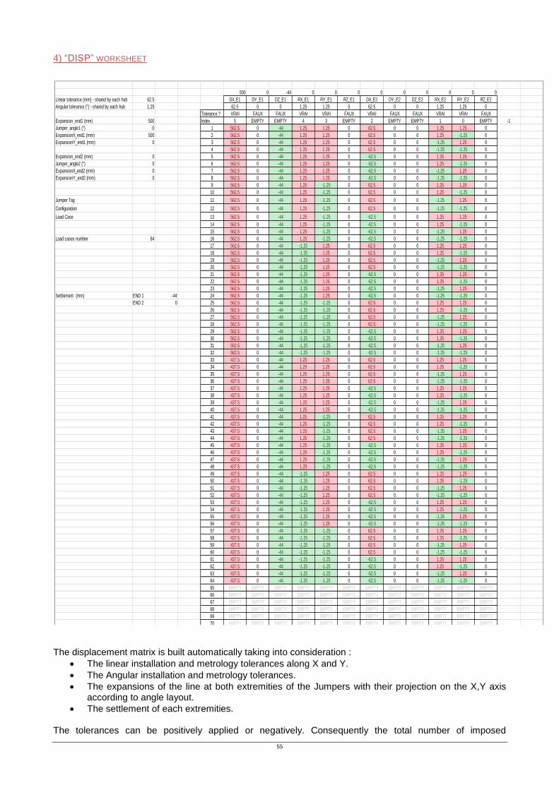
55

4) “DISP” WORKSHEET

The displacement matrix is built automatically taking into consideration :

The linear installation and metrology tolerances along X and Y.

The Angular installation and metrology tolerances.

The expansions of the line at both extremities of the Jumpers with their projection on the X,Y axis according to angle layout.

The settlement of each extremities. The tolerances can be positively applied or negatively. Consequently the total number of imposed

500 0 -44 0 0 0 0 0 0 0 0 0

Linear tolerance (mm) - shared by each hub 62.5 DX_E1 DY_E1 DZ_E1 RX_E1 RY_E1 RZ_E1 DX_E2 DY_E2 DZ_E2 RX_E2 RY_E2 RZ_E2

Angular tolerance (°) - shared by each hub 1.25 62.5 0 0 1.25 1.25 0 62.5 0 0 1.25 1.25 0

Tolerance ? VRAI FAUX FAUX VRAI VRAI FAUX VRAI FAUX FAUX VRAI VRAI FAUX

Expansion_end1 (mm) 500 Index 5 EMPTY EMPTY 4 3 EMPTY 2 EMPTY EMPTY 1 0 EMPTY -1

Jumper_angle1 (°) 0 1 562.5 0 -44 1.25 1.25 0 62.5 0 0 1.25 1.25 0

ExpansionX_end1 (mm) 500 2 562.5 0 -44 1.25 1.25 0 62.5 0 0 1.25 -1.25 0

ExpansionY_end1 (mm) 0 3 562.5 0 -44 1.25 1.25 0 62.5 0 0 -1.25 1.25 0

4 562.5 0 -44 1.25 1.25 0 62.5 0 0 -1.25 -1.25 0

Expansion_end2 (mm) 0 5 562.5 0 -44 1.25 1.25 0 -62.5 0 0 1.25 1.25 0

Jumper_angle2 (°) 0 6 562.5 0 -44 1.25 1.25 0 -62.5 0 0 1.25 -1.25 0

ExpansionX_end2 (mm) 0 7 562.5 0 -44 1.25 1.25 0 -62.5 0 0 -1.25 1.25 0

ExpansionY_end2 (mm) 0 8 562.5 0 -44 1.25 1.25 0 -62.5 0 0 -1.25 -1.25 0

9 562.5 0 -44 1.25 -1.25 0 62.5 0 0 1.25 1.25 0

10 562.5 0 -44 1.25 -1.25 0 62.5 0 0 1.25 -1.25 0

Jumper Tag 11 562.5 0 -44 1.25 -1.25 0 62.5 0 0 -1.25 1.25 0

Configuration 12 562.5 0 -44 1.25 -1.25 0 62.5 0 0 -1.25 -1.25 0

Load Case 13 562.5 0 -44 1.25 -1.25 0 -62.5 0 0 1.25 1.25 0

14 562.5 0 -44 1.25 -1.25 0 -62.5 0 0 1.25 -1.25 0

15 562.5 0 -44 1.25 -1.25 0 -62.5 0 0 -1.25 1.25 0

Load cases number 64 16 562.5 0 -44 1.25 -1.25 0 -62.5 0 0 -1.25 -1.25 0

17 562.5 0 -44 -1.25 1.25 0 62.5 0 0 1.25 1.25 0

18 562.5 0 -44 -1.25 1.25 0 62.5 0 0 1.25 -1.25 0

19 562.5 0 -44 -1.25 1.25 0 62.5 0 0 -1.25 1.25 0

20 562.5 0 -44 -1.25 1.25 0 62.5 0 0 -1.25 -1.25 0

21 562.5 0 -44 -1.25 1.25 0 -62.5 0 0 1.25 1.25 0

22 562.5 0 -44 -1.25 1.25 0 -62.5 0 0 1.25 -1.25 0

23 562.5 0 -44 -1.25 1.25 0 -62.5 0 0 -1.25 1.25 0

Settlement (mm) END 1 -44 24 562.5 0 -44 -1.25 1.25 0 -62.5 0 0 -1.25 -1.25 0

END 2 0 25 562.5 0 -44 -1.25 -1.25 0 62.5 0 0 1.25 1.25 0

26 562.5 0 -44 -1.25 -1.25 0 62.5 0 0 1.25 -1.25 0

27 562.5 0 -44 -1.25 -1.25 0 62.5 0 0 -1.25 1.25 0

28 562.5 0 -44 -1.25 -1.25 0 62.5 0 0 -1.25 -1.25 0

29 562.5 0 -44 -1.25 -1.25 0 -62.5 0 0 1.25 1.25 0

30 562.5 0 -44 -1.25 -1.25 0 -62.5 0 0 1.25 -1.25 0

31 562.5 0 -44 -1.25 -1.25 0 -62.5 0 0 -1.25 1.25 0

32 562.5 0 -44 -1.25 -1.25 0 -62.5 0 0 -1.25 -1.25 0

33 437.5 0 -44 1.25 1.25 0 62.5 0 0 1.25 1.25 0

34 437.5 0 -44 1.25 1.25 0 62.5 0 0 1.25 -1.25 0

35 437.5 0 -44 1.25 1.25 0 62.5 0 0 -1.25 1.25 0

36 437.5 0 -44 1.25 1.25 0 62.5 0 0 -1.25 -1.25 0

37 437.5 0 -44 1.25 1.25 0 -62.5 0 0 1.25 1.25 0

38 437.5 0 -44 1.25 1.25 0 -62.5 0 0 1.25 -1.25 0

39 437.5 0 -44 1.25 1.25 0 -62.5 0 0 -1.25 1.25 0

40 437.5 0 -44 1.25 1.25 0 -62.5 0 0 -1.25 -1.25 0

41 437.5 0 -44 1.25 -1.25 0 62.5 0 0 1.25 1.25 0

42 437.5 0 -44 1.25 -1.25 0 62.5 0 0 1.25 -1.25 0

43 437.5 0 -44 1.25 -1.25 0 62.5 0 0 -1.25 1.25 0

44 437.5 0 -44 1.25 -1.25 0 62.5 0 0 -1.25 -1.25 0

45 437.5 0 -44 1.25 -1.25 0 -62.5 0 0 1.25 1.25 0

46 437.5 0 -44 1.25 -1.25 0 -62.5 0 0 1.25 -1.25 0

47 437.5 0 -44 1.25 -1.25 0 -62.5 0 0 -1.25 1.25 0

48 437.5 0 -44 1.25 -1.25 0 -62.5 0 0 -1.25 -1.25 0

49 437.5 0 -44 -1.25 1.25 0 62.5 0 0 1.25 1.25 0

50 437.5 0 -44 -1.25 1.25 0 62.5 0 0 1.25 -1.25 0

51 437.5 0 -44 -1.25 1.25 0 62.5 0 0 -1.25 1.25 0

52 437.5 0 -44 -1.25 1.25 0 62.5 0 0 -1.25 -1.25 0

53 437.5 0 -44 -1.25 1.25 0 -62.5 0 0 1.25 1.25 0

54 437.5 0 -44 -1.25 1.25 0 -62.5 0 0 1.25 -1.25 0

55 437.5 0 -44 -1.25 1.25 0 -62.5 0 0 -1.25 1.25 0

56 437.5 0 -44 -1.25 1.25 0 -62.5 0 0 -1.25 -1.25 0

57 437.5 0 -44 -1.25 -1.25 0 62.5 0 0 1.25 1.25 0

58 437.5 0 -44 -1.25 -1.25 0 62.5 0 0 1.25 -1.25 0

59 437.5 0 -44 -1.25 -1.25 0 62.5 0 0 -1.25 1.25 0

60 437.5 0 -44 -1.25 -1.25 0 62.5 0 0 -1.25 -1.25 0

61 437.5 0 -44 -1.25 -1.25 0 -62.5 0 0 1.25 1.25 0

62 437.5 0 -44 -1.25 -1.25 0 -62.5 0 0 1.25 -1.25 0

63 437.5 0 -44 -1.25 -1.25 0 -62.5 0 0 -1.25 1.25 0

64 437.5 0 -44 -1.25 -1.25 0 -62.5 0 0 -1.25 -1.25 0

65 EMPTY EMPTY EMPTY EMPTY EMPTY EMPTY EMPTY EMPTY EMPTY EMPTY EMPTY EMPTY

66 EMPTY EMPTY EMPTY EMPTY EMPTY EMPTY EMPTY EMPTY EMPTY EMPTY EMPTY EMPTY

67 EMPTY EMPTY EMPTY EMPTY EMPTY EMPTY EMPTY EMPTY EMPTY EMPTY EMPTY EMPTY

68 EMPTY EMPTY EMPTY EMPTY EMPTY EMPTY EMPTY EMPTY EMPTY EMPTY EMPTY EMPTY

69 EMPTY EMPTY EMPTY EMPTY EMPTY EMPTY EMPTY EMPTY EMPTY EMPTY EMPTY EMPTY

70 EMPTY EMPTY EMPTY EMPTY EMPTY EMPTY EMPTY EMPTY EMPTY EMPTY EMPTY EMPTY

56

displacement cases is composed of : 2^6=64 cases. Combining all the extreme tolerances could result in very conservative stress and interface loads. Therefore a probability approach is sometimes used., assuming that all the individual tolerances follow a uniform distribution within the tolerance limit. The cumulative probability for the total tolerance can then be defined, as shown in Figure 47

Figure 47. Typical Cumulative Probability

As for the current thesis project, all the tolerances are conserved for testing in order to have a general design tool. In order to analyse each metrological configuration accurately, single Abaqus script files have been written including only one displacement load case. Indeed the plastic behaviour of the structure should not be reached to take correctly into account the load case.

57

5) “RESULTS” WORKSHEET

The “RESULTS” worksheet summarizes the stresses of ASME B31.8 and reaction loads at both extremities. The DNV checks are also performed in the same worksheet. All the load cases (As Landed, Hydrotest, Leak Test, Design, Operating and Shut Down) are completed into tables. Comparison between ABAQUS and AUTOPIPE can be done.

Stress Checks ASME B31.8, Platform Piping and Risers Reaction Forces and Moments @ End 1

1 Jumper Tag Load Case Value [MPa] Allow. [MPa] Ratio To analyse 1 Jumper Tag Load Case Structure Tag Fx(N) Fy(N) Fz(N) Mx(N.m) My(N.m) Mz(N.m) To analyse

Maximum Hoop Stress 0 225 0 11380 499.8 50840 27620 7032 8599

Maximum Longitudinal Stress 139.665325 360 0.39 -28970 -874.9 43510 -26350 -186300 -9194

Maximum Combined Stress 173.353156 405 0.43Maximum Hoop Stress 225 0

Maximum Longitudinal Stress 360 0 WIJ-04Maximum Combined Stress 405 0 NOM

Maximum Hoop Stress 225 0Maximum Longitudinal Stress 360 0

WIJ-04 Maximum Combined Stress 405 0 55620 356.8 51090 28070 153400 6748NOM Maximum Hoop Stress 225 0 15270 -1018 43770 -25890 -39980 -11040

Maximum Longitudinal Stress 360 0Maximum Combined Stress 405 0

Maximum Hoop Stress 122.350631 225 0.54Maximum Longitudinal Stress 297.331409 360 0.83Maximum Combined Stress 381.031902 405 0.94

Maximum Hoop Stress 225 0Maximum Longitudinal Stress 360 0Maximum Combined Stress 405 0

1 Jumper Tag Load Case Value [MPa] Allow. [MPa] Ratio To analyse 1 Jumper Tag Load Case Structure Tag Fx(N) Fy(N) Fz(N) Mx(N.m) My(N.m) Mz(N.m) To analyseMaximum Hoop Stress 0 225 0 Max 23956 880 -43610 24881 172555 9271

Maximum Longitudinal Stress 121.78 360 0.34 Min -8232 -504 -49738 -26149 3702 -8681Maximum Combined Stress 149.9 405 0.37 Max

Maximum Hoop Stress 225 0 MinMaximum Longitudinal Stress 360 0 WIJ-04 MaxMaximum Combined Stress 405 0 NOM Min

Maximum Hoop Stress 225 0 Max

Maximum Longitudinal Stress 360 0 Min

WIJ-04 Maximum Combined Stress 405 0 Max -9790 1013 -43795 24419 49690 11001

NOM Maximum Hoop Stress 225 0 Min -41978 -371 -49924 -26611 -119163 -6950

Maximum Longitudinal Stress 360 0 Max

Maximum Combined Stress 405 0 Min

Maximum Hoop Stress 122.35 225 0.54

Maximum Longitudinal Stress 248.28 360 0.69

Maximum Combined Stress 333.18 405 0.82

Maximum Hoop Stress 225 0

Maximum Longitudinal Stress 360 0

Maximum Combined Stress 405 0

Shut_Down

WFTA-04SHydrotest

AsLanded

A

U

T

O

P

I

P

E

A

B

A

Q

U

S

Operating WFTA-04S

0

1

0

0

0

1WFTA-04S

Design WFTA-04S

WFTA-04S

Leak_Test WFTA-04S

Design

1

0

0

0

Design

Operating

0

1

Shut_Down

1

0

WFTA-04S

WFTA-04S

WFTA-04S

WFTA-04S

WFTA-04S

Operating

AsLanded

Hydrotest

Leak_Test

1

0

0

WFTA-04SShut_Down 0

1

0

0

A

B

A

Q

U

S

A

U

T

O

P

I

P

E

Leak_Test

Design

Operating

Shut_Down 0

AsLanded

Hydrotest

Leak_Test

0

1

AsLanded

Hydrotest

Stress Checks ASME B31.8, Pipelines Stress Checks DNV

1 Jumper Tag Load Case Value [MPa] Allow. [MPa] Ratio To analyse 1 Jumper Tag Load Case To analyse

Maximum Hoop Stress 0 324 0 Maximum Axial Force 41.98

Maximum Longitudinal Stress 139.665325 360 0.39 Maximum Bending Moment 192.81632

Maximum Combined Stress 141.047623 405 0.35Maximum Hoop Stress 324 0 Maximum Axial Force

Maximum Longitudinal Stress 360 0 Maximum Bending MomentMaximum Combined Stress 405 0

Maximum Hoop Stress 324 0 Maximum Axial ForceMaximum Longitudinal Stress 360 0 Maximum Bending Moment

WIJ-04 Maximum Combined Stress 405 0 WIJ-04NOM Maximum Hoop Stress 324 0 NOM Maximum Axial Force

Maximum Longitudinal Stress 360 0 Maximum Bending MomentMaximum Combined Stress 405 0

Maximum Hoop Stress 122.350631 324 0.38 Maximum Axial Force 61.53Maximum Longitudinal Stress 297.331409 360 0.83 Maximum Bending Moment 337.97046Maximum Combined Stress 308.047253 405 0.76

Maximum Hoop Stress 324 0 Maximum Axial ForceMaximum Longitudinal Stress 360 0 Maximum Bending MomentMaximum Combined Stress 405 0

1 Jumper Tag Load Case Value [MPa] Allow. [MPa] Ratio To analyse 1 Jumper Tag Load Case To analyseMaximum Hoop Stress 0 324 0 Maximum Axial Force 41.489359

Maximum Longitudinal Stress 121.78 360 0.34 Maximum Bending Moment 180.30079Maximum Combined Stress 121.95945 405 0.3

Maximum Hoop Stress 324 0 Maximum Axial ForceMaximum Longitudinal Stress 360 0 Maximum Bending MomentMaximum Combined Stress 405 0

Maximum Hoop Stress 324 0 Maximum Axial Force

Maximum Longitudinal Stress 360 0 Maximum Bending Moment

WIJ-04 Maximum Combined Stress 405 0 WIJ-04

NOM Maximum Hoop Stress 324 0 NOM Maximum Axial Force

Maximum Longitudinal Stress 360 0 Maximum Bending Moment

Maximum Combined Stress 405 0

Maximum Hoop Stress 122.35 324 0.38 Maximum Axial Force 48.772444

Maximum Longitudinal Stress 248.28 360 0.69 Maximum Bending Moment 276.40575

Maximum Combined Stress 265.834651 405 0.66

Maximum Hoop Stress 324 0 Maximum Axial Force

Maximum Longitudinal Stress 360 0 Maximum Bending Moment

Maximum Combined Stress 405 0

Value [KN], [KN.m]

Value [KN], [KN.m]

A

U

T

O

P

I

P

E

AsLanded 1

Hydrotest 0

Leak_Test 0

Design 0

Operating 1

Shut_Down 0

A

B

A

Q

U

S

AsLanded 1

Hydrotest 0

Leak_Test 0

Design 0

Operating 1

Shut_Down 00

A

U

T

O

P

I

P

E

AsLanded 1

Hydrotest 0

Leak_Test 0

Design 0

Operating 1

Shut_Down 0

1

Hydrotest 0

Leak_Test 0

Design 0

Operating 1

A

B

A

Q

U

S

AsLanded

Shut_Down

58

4.2.1 Process Flowchart

The input spreadsheet is based on a VBA code that is taking the input variable and transferring their values into the two excel worksheets INP and NTL. Those worksheets have been developed so that each line of the Abaqus and Autopipe codes are parameterized by input variables. An extracting code is generating the *.INP and *.NTL files. Each of the directional arrow represents an excel button available to the user.

Create NTL Files and Run Autopipe Create INP Files and Run Abaqus

Start

INPT FILE

Create Path

Copy Input Spreadsheet in

the folders

Complete INP worksheets in each load case

Extract and create *.inp files

Each step *.inp file is created as well as LCFinal.inp

Create a *.bat file to launch

Abaqus analysis

Launch Abaqus analysis

Create Path

Copy Input Spreadsheet in

the folders

Complete NTL worksheets

in each load case

Extract and create *.ntl

files

*.NTL is created with all the displacement steps

Create a *.bat file to

launch Autopipe analysis

Launch Autopipe analysis

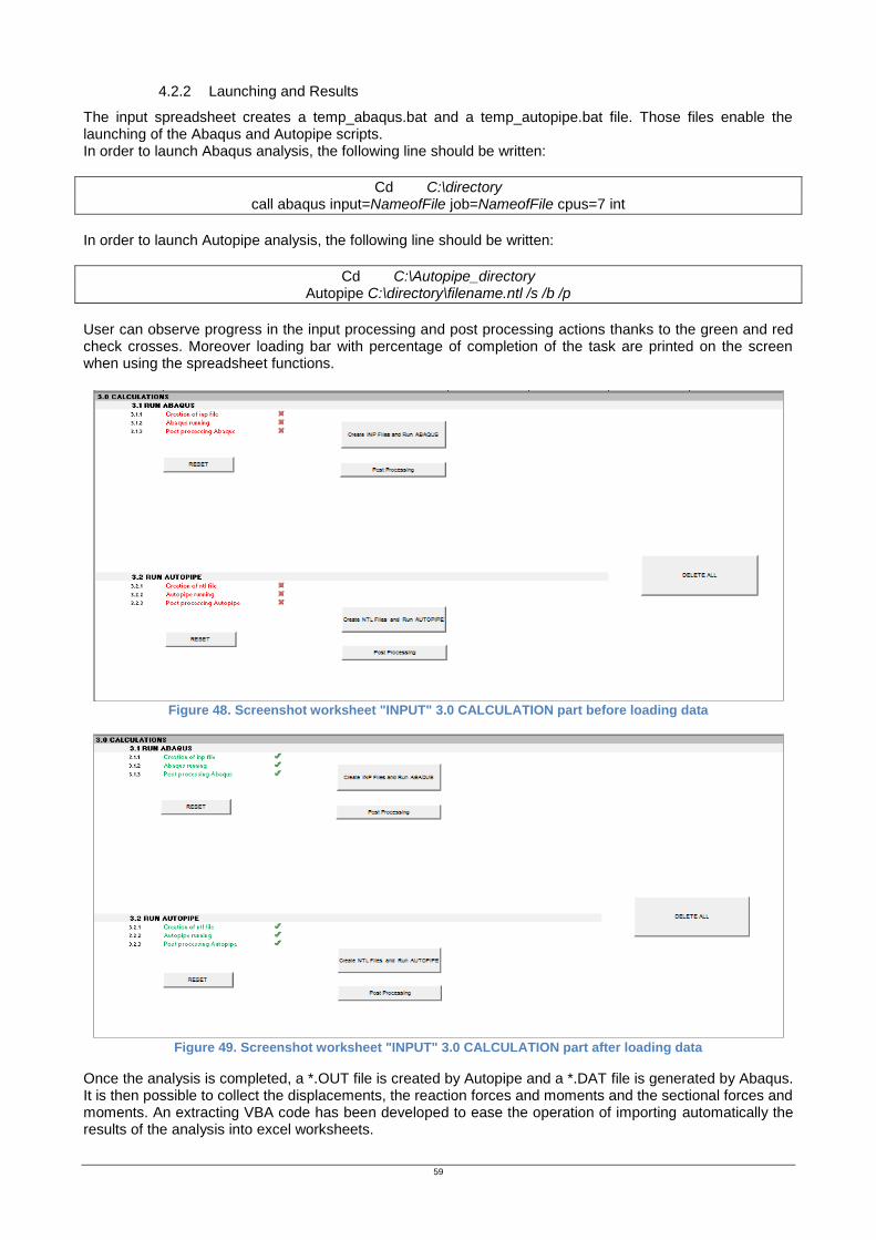
59

4.2.2 Launching and Results

The input spreadsheet creates a temp_abaqus.bat and a temp_autopipe.bat file. Those files enable the launching of the Abaqus and Autopipe scripts. In order to launch Abaqus analysis, the following line should be written:

Cd C:\directory call abaqus input=NameofFile job=NameofFile cpus=7 int

In order to launch Autopipe analysis, the following line should be written:

Cd C:\Autopipe_directory Autopipe C:\directory\filename.ntl /s /b /p

User can observe progress in the input processing and post processing actions thanks to the green and red check crosses. Moreover loading bar with percentage of completion of the task are printed on the screen when using the spreadsheet functions.

Figure 48. Screenshot worksheet "INPUT" 3.0 CALCULATION part before loading data

Figure 49. Screenshot worksheet "INPUT" 3.0 CALCULATION part after loading data

Once the analysis is completed, a *.OUT file is created by Autopipe and a *.DAT file is generated by Abaqus. It is then possible to collect the displacements, the reaction forces and moments and the sectional forces and moments. An extracting VBA code has been developed to ease the operation of importing automatically the results of the analysis into excel worksheets.

60

The post processing is done thanks to the import data options of excel. Indeed starting from the FEA program outputs, a VBA code create text files that can easily be imported into excel. Then the post processing VBA code (see Attachement C) orders the data of each variable (displacement along X, Sectional Force Y…) into tables in order to compute the maximum values. Additionally mathematical operations are carried on, to obtain the ASME and DNV code checks. Those operations have been described in 3.1.2, their practical applications will be details in the part 3.3 of this report.

4.2.3 Abaqus Files

When the run of the solver begins, i.e., the sentence “Run standard.exe” appears on the command window, Abaqus analysis starts. At the same time, in the folder where all the input files are saved, the following new files are created:

Figure 50. Screenshot Abaqus command windows, the solver begins to run

NameJumper_Config_loadcaseLCFinal.com Command file, created by the Abaqus execution procedure

NameJumper_Config_loadcaseLCFinal.dat Printed output file. It is written by the analysis, data check and parameter check option.

NameJumper_Config_loadcaseLCFinal.lck

Lock file for the output database. This file is written whenever an output database file is opened with write access; it prevents you from having simultaneous write permission to the output database from multiple sources. It is deleted automatically when the output database file is closed or when the analysis that creates it ends.

NameJumper_Config_loadcaseLCFinal.msg Message file.

NameJumper_Config_loadcaseLCFinal.odb

Output database. It is written by the analysis and continue options in Abaqus/Standard and Abaqus/Explicit. It is read by the Visualization module in Abaqus/CAE (Abaqus/Viewer) and by the convert=odb option. This file is required for restart.

NameJumper_Config_loadcaseLCFinal.par Modified version of original parameterized input file showing input parameters and their values.

NameJumper_Config_loadcaseLCFinal.pes Modified version of original parameterized input file showing input free of parameter information (after input parameter evaluation and substitution has been performed).

NameJumper_Config_loadcaseLCFinal.pmg Parameter evaluation and substitution message file. It is written when the input file is parameterized.

NameJumper_Config_loadcaseLCFinal.prt

Part file, used by Abaqus/Standard and Abaqus/Explicit. This file is used to store part and assembly information and is created even if the input file does not contain an assembly definition. The part file is required for restart, import, sequentially coupled thermal-stress analysis, symmetric model generation, and underwater shock analysis, even if the model is not defined in terms of an assembly of part instances. This file may also be needed for sub-modelling

61

analysis.

NameJumper_Config_loadcaseLCFinal.sim

Linear dynamics data file, used by Abaqus/Standard. It is written during the frequency extraction procedure in SIM-based linear dynamics analyses and is used to store eigenvectors, substructure matrices, and other modal system information. This file is required for restart. Model file, used by Abaqus/CFD. It is written by the data check option. It is read and can be written by the analysis and continue options. This file is required for restart.

NameJumper_Config_loadcaseLCFinal.sta Status file. Abaqus writes increment summaries to this file in the analysis, continue, and recover options.

The post processing code will extract relevant data from the *.DAT file.

4.2.4 Autopipe Files

When the run of the solver begins, Autopipe analysis starts. At the same time, in the folder where all the input files are saved, the following new files are created :

Figure 51. Screenshot Autopipe command windows, the solver begins to run

NameJumper_Config_loadcaseLCFinal.OUT The Result Output Report which contains the outputs data.

NameJumper_Config_loadcaseLCFinal.dat The Model File that could be open with AUTOPIPE software to verify the geometry.

NameJumper_Config_loadcaseLCFinal.MSG The Message File which contains the possible warnings and errors of the analysis.

NameJumper_Config_loadcaseLCFinal.LOG This file can be used to identify the support(s) which failed to converge.

NameJumper_Config_loadcaseLCFinal.CMB This is the model combination file.

NameJumper_Config_loadcaseLCFinal.CHK This is the Model Consistency Check.

The post processing code will extract relevant data from the *.OUT file.

4.3 POST PROCESSING SPREADSHEETS

The purpose of those spreadsheets (FORM-SSA-SFD-FLOWS-055-E & FORM-SSA-SFD-FLOWS-056-E) is:

To load the output data of Abaqus and Autopipe analysis.

To calculate mechanical parameters of the Jumper (section modulus, areas, end cap effects)

To compute the Stresses required by the standards and isolate the maximum values.

62

To draw out the graphs of the displacements, forces, moments, stresses along the Jumper

VBA code has been used to automatize the post processing starting from the *.DAT and *.OUT files respectively from Abaqus and Autopipe. (see Attachement D). For each Jumper and each configuration a different spreadsheet will be completed.

Standard quality requirements of the Flowline Department of Saipem have been respected. The spreadsheet is composed of 9 main worksheets:

COVER PAGE, REVISION HISTORY, OUTPUTS, INPUTS, GRAPHS, DISPLACEMENTS, REACTIONS, FORCES&MOMENTS, STRESSES

63

1) “COVER PAGE” WORKSHEET

/

This document is t he p ropert y o f t he C ON TR A C TOR who wil l saf eguard it s r ight s accord ing t o t he civil and penal p rovisions o f t he law.

PREPAREDREV. DATE DESCRIPTION CHECKED APPROVED

41

ABAQUS / AUTOPIPE POST PROCESSING SPREADSHEET M-SHAPED JUMPERS

DateRev.WBSCLIENT

CLIENT PROJECT TITLE

CLIENT

Doc. N°

CONTRACTOR

Job / Doc. N°

LOCATION

Project TitleLocation

Status PageDoc. Title Doc. ClassABAQUS / AUTOPIPE POST PROCESSING SPREADSHEET M-SHAPED

JUMPERS

64

2) “REVISION HISTORY” WORKSHEET

/

REVISION HISTORY

List of HOLDs

This document is t he p ropert y o f t he C ON TR A C TOR who wil l saf eguard it s r ight s accord ing t o t he civil and penal p rovisions o f t he law.

9

10

7

8

5

6

3

4

CLIENT PROJECT TITLE

1

2

Page

Update / Amendment Details

42

CLIENT Project TitleLocation Rev.

CLIENT

Doc. N°

CONTRACTOR

Job / Doc. N°

DateWBS

Rev. Status Date

ABAQUS / AUTOPIPE POST PROCESSING SPREADSHEET M-SHAPED

JUMPERS

Doc. Title

LOCATIONStatusDoc. Class

PageHOLD DescriptionN°

65

3) “OUTPUTS” WORKSHEET

The worksheet is completed for each load case. The tables summarize the stresses, forces and displacements obtained by the FEA programs. The VBA code isolating those values is based on the ordering of the output variables into tables and the computation of the maximum values in those tables. The maximum deflection along Z should be checked with the seabed clearance in order to make sure that the jumper is not laying on the seabed.

Location

LOCATION

4.0 OUTPUTS

4.1 Files and Identification

4.1.1 Base Folder

4.1.2 Input file Spreadsheet

4.1.3 Post processing AUTOPIPE Spreadsheet

4.1.4 Jumper Tag Jumper_tag

4.1.5 Configuration Config

4.1.6 Load Case load_case

4.2 Load data & calculations

4.2.1Displacements 100

4.2.2Reactions 100

4.2.3Forces & Moments 100

4.2.4Stresses 100

4.3 Summary Results Units

4.3.1 Maximum Stresses

4.3.1.1 Maximum Hoop Stress Mpa [_] 122.35 122.35

4.3.1.2 Maximum Longitudinal Stress Mpa [_] 248.28 248.28

4.3.1.3 Maximum Combined Stress Mpa [_] 333.18 265.834651

4.3.2 Maximum Stresses with Bend Thining

4.3.2.1 Maximum Hoop Stress Mpa [_] 202.432953 202.432953

4.3.2.2 Maximum Longitudinal Stress Mpa [_] 248.28 248.28

4.3.2.3 Maximum Combined Stress Mpa [_] 376.399826 345.906793

4.3.3 Maximum Reaction Forces & Moments at End 1

4.3.3.1 Force X force_X_end1 N [_] -9790

4.3.3.2 Force Y force_Y_end1 N [_] 1013

4.3.3.3 Force Z force_Z_end1 N [_] -43795

4.3.3.4 Moment X moment_X_end1 N.m [_] 24419

4.3.3.5 Moment Y moment_Y_end1 N.m [_] 49690

4.3.3.6 Moment Z moment_Z_end1 N.m [_] 11001

4.3.4 Maximum Reaction Forces & Moments at End 2

4.3.4.1 Force X force_X_end2 N [_] 41978

4.3.4.2 Force Y force_Y_end2 N [_] 747

4.3.4.3 Force Z force_Z_end2 N [_] -44441

4.3.4.4 Moment X moment_X_end2 N.m [_] 25461

4.3.4.5 Moment Y moment_Y_end2 N.m [_] 123656

4.3.4.6 Moment Z moment_Z_end2 N.m [_] 10297

4.3.6 Maximum Displacements

4.3.6.1 Displacement X mm [_] 468.52

4.3.6.2 Displacement Y mm [_] -115.08

4.3.6.3 Displacement Z mm [_] -98.2

4.3.7 Minimum Displacements

4.3.7.1 Displacement X mm [_] -524.38

4.3.7.2 Displacement Y mm [_] -446.11

4.3.7.3 Displacement Z mm [_] -482.54

4.3.8 Minimum Reaction Forces & Moments at End 1

4.3.8.1 Force X force_X_end1 N [_] -41978

4.3.8.2 Force Y force_Y_end1 N [_] -371

4.3.8.3 Force Z force_Z_end1 N [_] -49924

4.3.8.4 Moment X moment_X_end1 N.m [_] -26611

4.3.8.5 Moment Y moment_Y_end1 N.m [_] -119163

4.3.8.6 Moment Z moment_Z_end1 N.m [_] -6950

4.3.9 Minimum Reaction Forces & Moments at End 2

4.3.9.1 Force X force_X_end1 N [_] 9790

4.3.9.2 Force Y force_Y_end1 N [_] -637

4.3.9.3 Force Z force_Z_end1 N [_] -50570

4.3.9.4 Moment X moment_X_end1 N.m [_] -25809

4.3.9.5 Moment Y moment_Y_end1 N.m [_] -48272

4.3.9.6 Moment Z moment_Z_end1 N.m [_] -7453

4.3.10 DNV checks

4.3.10.1 Maximum Axial Force KN [_] 48.7724438

4.3.10.2 Minimum Axial Force KN [_] -25.8151672

4.3.10.3 Maximum Bending Moment KN.m [_] 276.40575

4.3.10.4 Minimum Bending Moment KN.m [_] 0.27351109

4.3.10.5 Maximum ABS Axial Force KN [_] 48.7724438

4.3.10.6 Maximum ABS Bending Moment KN.m [_] 276.40575

5.0 GRAPHS

See 5.0 Graphs

CLIENT

CLIENTDoc.Title

DOCUMENT TITLE

PROJECT TITLE

Project Title WBS Rev Date

CLIENT Doc. N°

CONTRACTOR Job / Doc. N°

0

0

Doc. Class Status Page

3 /4

Riser Plat.

ASME B31.8

Pipeline

ASME B31.8

NOM

OPERATING

C:\users-data\saf100298\Contacts\Desktop\DevlopmentSpreadsheet\04082014

WIJ-04

FORM-SSA-SFD-FLOWS-055-E

FORM-SSA-SFD-FLOWS-054-E

LOAD DATACALCULATE

LOAD JUMPERS

Reset

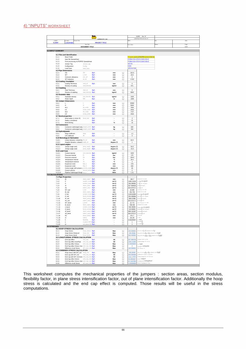
66

4) “INPUTS” WORKSHEET

This worksheet computes the mechanical properties of the jumpers : section areas, section modulus, flexibility factor, in plane stress intensification factor, out of plane intensification factor. Additionally the hoop stress is calculated and the end cap effect is computed. Those results will be useful in the stress computations.

Location

LOCATION

6.0 INPUT SUMMARY

6.1 Files and Identification

6.1.1 Base Folder

6.1.2 Input file Spreadsheet

6.1.3 Post processing AUTOPIPE Spreadsheet

6.1.4 Jumper Tag Jumper_tag

6.1.5 Configuration Config

6.1.6 Load Case load_case

6.2 Pipe Dimensions

6.2.1 OD OD Ref : mm [_] 323.9

6.2.2 WT t_nom Ref : mm [_] 20.6

6.2.3 Corrosion allowance corr_all Ref : mm [_] 0

6.2.4 WT tolerance wt_tol Ref : mm [_] 4.532

6.3 Coating / Insulation

6.3.1 Coating Thickness coat_wt Ref : mm [_] 0

6.3.2 Density of coating coat_density kg/m3 [_] 671

6.4 Cladding

6.4.1 Clad Thickness clad_wt Ref : mm [_] 0

6.4.2 Density of cladding clad_density Ref : kg/m3 [_] 8840

6.5 Seawater data

6.5.1 Seawater density sea_desnity Ref : kg/m3 [_] 1025

6.5.2 Water depth WD Ref : m [_] 1098

6.6 Jumper Dimensions

6.6.1 L L Ref : mm [_] 25800

6.6.2 H H Ref : mm [_] 8500

6.6.3 Hc1 Hc_end1 Ref : mm [_] 7554

6.6.4 Ll1 Lloop_end1 Ref : mm [_] 2916

6.6.5 Hc2 Hc_end2 Ref : mm [_] 7727

6.6.6 Ll2 Lloop_end2 Ref : mm [_] 2916

6.7 Bend properties

6.7.1 Bend radius (x times D) bend_rad Ref : - [_] 3

6.7.2 Radius considered Ref : - [_] ID

6.7.3 Bend thining Ref : % [_] 16

6.8 Connectors

6.8.1 Connector submerged weight -end1weight_end1 Ref : kg [_] 964

6.8.2 Connector submerged weight -end2weight_end2 Ref : kg [_] 964

6.9 Hydrodynamic

6.9.1 Drag coefficient drag Ref : - [_] 1.2

6.9.2 Lift coefficient lift Ref : - [_] 0

6.10 Metrology & Fabrication

6.10.1 Linear tolerance -shared by each endlinr_tol Ref : mm [_] 62.5

6.10.2 Angular tolerance -shared by each endanglr_tol Ref : degree (°) [_] 1

6.11 Layout angles

6.11.1 Jumper angle end1 jump_angl1 Ref : degree (°) [_] 50.9

6.11.2 Jumper angle end2 jump_angl2 Ref : degree (°) [_] -42.5

6.12 Load Case

6.12.1 Content density cont_density Ref : kg/m3 [_] 1025

6.12.2 Pressure internal Pi Ref : bar [_] 276

6.12.3 Pressure external Pe Ref : bar [_] 109.8

6.12.4 Temperature internal Ti Ref : °C [_] 26.5

6.12.5 Temperature external Te Ref : °C [_] 4

6.12.6 Expansion end1 Exp_1 Ref : mm [_] 379

6.12.7 Expansion end2 Exp_2 Ref : mm [_] 400

6.12.8 Current angle with jumper planecurrent_angle Ref : degree (°) [_] 90

6.12.9 Current velocity current_velocityRef : m/s [_] 0

6.12.10 Pipeline Submerged Weight (Operating)sw_o Ref : kN/m [_] 1.31

7.0 CALCULATIONS

7.1 Pipe Properties

7.1.1 ID intern_diam Ref : mm [_] 282.7

7.1.2 Z section_modulRef : cm^3 [_] 1400.11016

7.1.3 A section_area Ref : cm^2 [_] 196.286081

7.1.4 Ai intern_area Ref : cm^2 [_] 627.684636

7.1.5 Ae extern_area Ref : cm^2 [_] 823.970717

7.1.6 WT_red t_red Ref : mm [_] 16.068

7.1.7 ID_red intern_diam_redRef : mm [_] 291.764

7.1.8 Z_red section_modulRef : cm^3 [_] 1139.62955

7.1.9 A_red bend_section_redRef : cm^2 [_] 155.390856

7.1.10 Ai_red intern_area_redRef : cm^2 [_] 668.57986

7.1.11 Ae_red extern_area_redRef : cm^2 [_] 823.970717

7.1.12 WT_bend t_bend Ref : mm [_] 12.772

7.1.13 ID_bend intern_diam_bendRef : mm [_] 298.356

7.1.14 Z_bend section_modul_bendRef : cm^3 [_] 934.30005

7.1.15 A_bend bend_section_bendRef : cm^2 [_] 124.83831

7.1.16 Ai_bend intern_area_bendRef : cm^2 [_] 699.132407

7.1.17 Ae_bend extern_area_bendRef : cm^2 [_] 823.970717

7.1.18 R1 bend_radius Ref : mm [_] 971.7

7.1.19 r2 radius Ref : mm [_] 161.95

7.1.20 h flexibility Ref : - [_] 0.00295567

7.1.21 ii in-plane SIF B31.8Ref : - [_] 1

7.1.22 io out_plane SIF B31.8Ref : - [_] 1

8.0 STRESSES

8.1 HOOP STRESS CALCULATION

8.1.1 Hoop Stress hoop_stress Ref : Mpa [_] 122.350631

8.1.2 Hoop Stress Reduced hoop_red Ref : Mpa [_] 159.20363

8.1.3 Hoop Stress Bend hoop_bend Ref : Mpa [_] 202.432953

8.2 LONGITUDINAL STRESS CALCULATION

8.2.1 End Cap effect end_cap Ref : kN [_] 827.689748

8.2.2 End Cap effect AutoPipe end_cap_autopRef : kN [_] 1043.21186

8.2.3 End Cap effect Stress end_cap_stressRef : Mpa [_] 0.05094605

8.2.4 End Cap effect Stress Autopipeend_cap_stress_autopipeRef : Mpa [_] 0

8.2.5 Difference Axial Stress diff_axial_stressRef : Mpa [_] 122.350631

8.3 COMBINED STRESS CALCULATION

8.3.1 Hoop stress with WT_red hoop_red Ref : Mpa [_] 159.20363

8.3.2 End cap with WT_red end_cap_red Ref : kN [_] 940.560568

8.3.3 End cap with WT_red Autopipeend_cap_red_autoRef : kN [_] 1111.17973

8.3.4 End Cap effect Stress end_cap_stressRef : Mpa [_] 53.2650227

8.3.5 End Cap effect Stress Autopipeend_cap_stress_autopipeRef : Mpa [_] 67.1347009

8.3.6 Difference Axial Stress diff_axial_stressRef : Mpa [_] -0.05094605

Doc. Class

4 /4

CLIENT Doc. N°

CONTRACTOR Job / Doc. N°

Date

Page

Rev

Status

NOM

OPERATING

Project Title WBS

WIJ-04

PROJECT TITLE

DOCUMENT TITLE

C:\users-data\saf100298\Contacts\Desktop\DevlopmentSpreadsheet\04082014

FORM-SSA-SFD-FLOWS-054-E

FORM-SSA-SFD-FLOWS-055-E

CLIENT

CLIENTDoc.Title

67

5) “GRAPHS” WORKSHEET

Variable variations along the jumper are been plotted simply for information purposes. Effective axial force, displacement DX, DY and DZ, Sectional forces SF1,SF2 and SF3 as well as sectional moments SM1,SM2 and SM3, Combined and Longitudinal Stresses are all gathered into graphs automatically.

CLIENT Location

CLIENT Location CLIENT Location CLIENT Location CLIENT Location 0 0

CLIENT LOCATION 0 0 0 0 0 0

5.9 Displacement Z

5.1 Sectional Force 1 5.2 Sectional Force 2 5.3 Sectional Force 3 5.7 Displacement X

CLIENT Location CLIENT Location CLIENT Location CLIENT Location CLIENT Location

0 0 0 0 0 0 0 0 0 0

5.4 Sectional Moment 1 5.5 Sectional Moment 2 5.6 Sectional Moment 3 5.8 Displacement Y 5.10 Longitudinal Stress

CONTRACTOR Job / Doc. N°

CLIENT Location Pro ject Title WBS Rev Date

0 0 0 0-Jan-00

Doc.Title Doc. Class Status Page

0 3 /5

5.11 Combined Stress

CONTRACTOR Job / Doc. N°

Pro ject Title WBS Rev Date

0 0-Jan-00Project Title WBS Rev Date

PROJECT TITLE

CLIENT Doc. N°

CONTRACTOR Job / Doc. N°

CLIENT Doc. N°

CONTRACTOR Job / Doc. N°

Doc.Title Doc. Class Status Page

Project Title WBS Rev Date

0 0-Jan-00

CLIENT Doc. N°

CONTRACTOR Job / Doc. N°

Page

/ 3 /5

Project Title WBS Rev Date

0 0-Jan-00

CLIENT Doc. N°

CONTRACTOR Job / Doc. N°

Doc.Title Doc. Class Status

0 3 /5

Doc.Title Doc. Class Status Page

DOCUMENT TITLE 3 /5

CLIENT Doc. N°

0 3 /5

Project Title WBS Rev Date

Doc.Title Doc. Class Status Page

0 3 /5

Project Title WBS Rev Date

0 0-Jan-00

0 3 /5

Project Title WBS Rev Date

0 0-Jan-00

Doc. Class Status PageDoc.Title

CLIENT Doc. N°

CONTRACTOR Job / Doc. N°

CLIENT Doc. N°

CONTRACTOR Job / Doc. N°

Doc.Title Doc. Class Status Page

0 3 /5

Project Title WBS Rev Date

0 0-Jan-00

CONTRACTOR Job / Doc. N°

Doc.Title Doc. Class Status Page

CONTRACTOR Job / Doc. N°

0 0-Jan-00 Doc.Title Doc. Class Status Page

0 3 /5

0-Jan-00

3 /5

CLIENT Doc. N°

Project Title WBS

CLIENT Doc. N°

CONTRACTOR Job / Doc. N°

Pro ject Title WBS Rev Date Rev Date

CLIENT Doc. N°

0 0-Jan-00

Doc.Title Doc. Class Status Page

0 3 /5

Doc.Title Doc. Class Status Page

0

0

-20000.00

-10000.00

0.00

10000.00

20000.00

30000.00

40000.00

50000.00

60000.00

0.00 10000.00 20000.00 30000.00 40000.00 50000.00 60000.00

KP [mm]

FX [N]

Série1

Série2

Série3

Série4

Série5

Série6

Série7

Série8

Série9

Série10

Série11

Série12

Série13

Série14

Série15

Série16

Série17

Série18

Série19

Série20

Série21

Série22

Série23

Série24

Série25

Série26

Série27

Série28

Série29

Série30

Série31

Série32

Série33

Série34

Série35

Série36

Série37

Série38

Série39

Série40

Série41

Série42

Série43

Série44

Série45

Série46

Série47

Série48

Série49

Série50

Série51

Série52

Série53

Série54

Série55

Série56

Série57

Série58

Série59

Série60

Série61

Série62

Série63

Série64

Série65

Série66

-1000.00

-800.00

-600.00

-400.00

-200.00

0.00

200.00

400.00

600.00

800.00

0.00 10000.00 20000.00 30000.00 40000.00 50000.00 60000.00

KP [mm]

FY [N]

Série1

Série2

Série3

Série4

Série5

Série6

Série7

Série8

Série9

Série10

Série11

Série12

Série13

Série14

Série15

Série16

Série17

Série18

Série19

Série20

Série21

Série22

Série23

Série24

Série25

Série26

Série27

Série28

Série29

Série30

Série31

Série32

Série33

Série34

Série35

Série36

Série37

Série38

Série39

Série40

Série41

Série42

Série43

Série44

Série45

Série46

Série47

Série48

Série49

Série50

Série51

Série52

Série53

Série54

Série55

Série56

Série57

Série58

Série59

Série60

Série61

Série62

Série63

Série64

Série65

Série66

-50000.00

-40000.00

-30000.00

-20000.00

-10000.00

0.00

10000.00

20000.00

30000.00

40000.00

50000.00

60000.00

0.00 10000.00 20000.00 30000.00 40000.00 50000.00 60000.00

KP [mm]

FZ [N]

Série1

Série2

Série3

Série4

Série5

Série6

Série7

Série8

Série9

Série10

Série11

Série12

Série13

Série14

Série15

Série16

Série17

Série18

Série19

Série20

Série21

Série22

Série23

Série24

Série25

Série26

Série27

Série28

Série29

Série30

Série31

Série32

Série33

Série34

Série35

Série36

Série37

Série38

Série39

Série40

Série41

Série42

Série43

Série44

Série45

Série46

Série47

Série48

Série49

Série50

Série51

Série52

Série53

Série54

Série55

Série56

Série57

Série58

Série59

Série60

Série61

Série62

Série63

Série64

Série65

Série66

-30000.00

-20000.00

-10000.00

0.00

10000.00

20000.00

30000.00

0.00 10000.00 20000.00 30000.00 40000.00 50000.00 60000.00

KP [mm]

MX [N.m]

Série1

Série2

Série3

Série4

Série5

Série6

Série7

Série8

Série9

Série10

Série11

Série12

Série13

Série14

Série15

Série16

Série17

Série18

Série19

Série20

Série21

Série22

Série23

Série24

Série25

Série26

Série27

Série28

Série29

Série30

Série31

Série32

Série33

Série34

Série35

Série36

Série37

Série38

Série39

Série40

Série41

Série42

Série43

Série44

Série45

Série46

Série47

Série48

Série49

Série50

Série51

Série52

Série53

Série54

Série55

Série56

Série57

Série58

Série59

Série60

Série61

Série62

Série63

Série64

Série65

Série66

-300000.00

-200000.00

-100000.00

0.00

100000.00

200000.00

300000.00

0.00 10000.00 20000.00 30000.00 40000.00 50000.00 60000.00

KP [mm]

MY [N.m]

Série1

Série2

Série3

Série4

Série5

Série6

Série7

Série8

Série9

Série10

Série11

Série12

Série13

Série14

Série15

Série16

Série17

Série18

Série19

Série20

Série21

Série22

Série23

Série24

Série25

Série26

Série27

Série28

Série29

Série30

Série31

Série32

Série33

Série34

Série35

Série36

Série37

Série38

Série39

Série40

Série41

Série42

Série43

Série44

Série45

Série46

Série47

Série48

Série49

Série50

Série51

Série52

Série53

Série54

Série55

Série56

Série57

Série58

Série59

Série60

Série61

Série62

Série63

Série64

Série65

Série66

-15000.00

-10000.00

-5000.00

0.00

5000.00

10000.00

15000.00

0.00 10000.00 20000.00 30000.00 40000.00 50000.00 60000.00

KP [mm]

MZ [N.m]

Série1

Série2

Série3

Série4

Série5

Série6

Série7

Série8

Série9

Série10

Série11

Série12

Série13

Série14

Série15

Série16

Série17

Série18

Série19

Série20

Série21

Série22

Série23

Série24

Série25

Série26

Série27

Série28

Série29

Série30

Série31

Série32

Série33

Série34

Série35

Série36

Série37

Série38

Série39

Série40

Série41

Série42

Série43

Série44

Série45

Série46

Série47

Série48

Série49

Série50

Série51

Série52

Série53

Série54

Série55

Série56

Série57

Série58

Série59

Série60

Série61

Série62

Série63

Série64

Série65

Série66

-600.00

-400.00

-200.00

0.00

200.00

400.00

600.00

0.00 10000.00 20000.00 30000.00 40000.00 50000.00 60000.00

KP [mm]

DX [m]

Série1

Série2

Série3

Série4

Série5

Série6

Série7

Série8

Série9

Série10

Série11

Série12

Série13

Série14

Série15

Série16

Série17

Série18

Série19

Série20

Série21

Série22

Série23

Série24

Série25

Série26

Série27

Série28

Série29

Série30

Série31

Série32

Série33

Série34

Série35

Série36

Série37

Série38

Série39

Série40

Série41

Série42

Série43

Série44

Série45

Série46

Série47

Série48

Série49

Série50

Série51

Série52

Série53

Série54

Série55

Série56

Série57

Série58

Série59

Série60

Série61

Série62

Série63

Série64

Série65

Série66

-500.00

-450.00

-400.00

-350.00

-300.00

-250.00

-200.00

-150.00

-100.00

-50.00

0.00

50.00

0.00 10000.00 20000.00 30000.00 40000.00 50000.00 60000.00

KP [mm]

DY [mm]

Série1

Série2

Série3

Série4

Série5

Série6

Série7

Série8

Série9

Série10

Série11

Série12

Série13

Série14

Série15

Série16

Série17

Série18

Série19

Série20

Série21

Série22

Série23

Série24

Série25

Série26

Série27

Série28

Série29

Série30

Série31

Série32

Série33

Série34

Série35

Série36

Série37

Série38

Série39

Série40

Série41

Série42

Série43

Série44

Série45

Série46

Série47

Série48

Série49

Série50

Série51

Série52

Série53

Série54

Série55

Série56

Série57

Série58

Série59

Série60

Série61

Série62

Série63

Série64

Série65

Série66

-600.00

-500.00

-400.00

-300.00

-200.00

-100.00

0.00

100.00

0.00 10000.00 20000.00 30000.00 40000.00 50000.00 60000.00

KP [mm]

DZ [m]

Série1

Série2

Série3

Série4

Série5

Série6

Série7

Série8

Série9

Série10

Série11

Série12

Série13

Série14

Série15

Série16

Série17

Série18

Série19

Série20

Série21

Série22

Série23

Série24

Série25

Série26

Série27

Série28

Série29

Série30

Série31

Série32

Série33

Série34

Série35

Série36

Série37

Série38

Série39

Série40

Série41

Série42

Série43

Série44

Série45

Série46

Série47

Série48

Série49

Série50

Série51

Série52

Série53

Série54

Série55

Série56

Série57

Série58

Série59

Série60

Série61

Série62

Série63

Série64

Série65

Série66

0.00

50.00

100.00

150.00

200.00

250.00

300.00

0.00 10000.00 20000.00 30000.00 40000.00 50000.00 60000.00

KP [mm]

Longitudinal Stress [MPa]

Série1

Série2

Série3

Série4

Série5

Série6

Série7

Série8

Série9

Série10

Série11

Série12

Série13

Série14

Série15

Série16

Série17

Série18

Série19

Série20

Série21

Série22

Série23

Série24

Série25

Série26

Série27

Série28

Série29

Série30

Série31

Série32

Série33

Série34

Série35

Série36

Série37

Série38

Série39

Série40

Série41

Série42

Série43

Série44

Série45

Série46

Série47

Série48

Série49

Série50

Série51

Série52

Série53

Série54

Série55

Série56

Série57

Série58

Série59

Série60

Série61

Série62

Série63

Série64

Série65

Série66

Série67

Série68

Série69

Série70

Série71

0.00

50.00

100.00

150.00

200.00

250.00

300.00

350.00

0.00 10000.00 20000.00 30000.00 40000.00 50000.00 60000.00

KP [mm]

Combined Stress [MPa]

Série1

Série2

Série3

Série4

Série5

Série6

Série7

Série8

Série9

Série10

Série11

Série12

Série13

Série14

Série15

Série16

Série17

Série18

Série19

Série20

Série21

Série22

Série23

Série24

Série25

Série26

Série27

Série28

Série29

Série30

Série31

Série32

Série33

Série34

Série35

Série36

Série37

Série38

Série39

Série40

Série41

Série42

Série43

Série44

Série45

Série46

Série47

Série48

Série49

Série50

Série51

Série52

Série53

Série54

Série55

Série56

Série57

Série58

Série59

Série60

Série61

Série62

Série63

Série64

Série65

Série66

Série67

Série68

Série69

Série70

Série71

68

6) “DISPLACEMENTS” WORKSHEET

The importing options on excel has enabled to save the displacements and rotations for all the nodes of the model and all the load cases. The data can be used to check the results and the deformed shape of the pipeline. The maximum values are extracted and transferred in the OUTPUTS worksheet.

Point Load TRANSLATIONS (mm) ROTATIONS (deg)

name combination X Y Z X Y Z

------ ----------------------- ------ ------ ------ ------- ------- -------

A00 Gravity{1} 0 0 0 0 0 0

User 1{1} 0 0 0 0 0 0

Thermal 1{1} 301.53 -294.12 -106 1 1 0

Thermal 2{1} 301.53 -294.12 -106 1 1 0

Thermal 3{1} 301.53 -294.12 -106 1 1 0

Thermal 4{1} 301.53 -294.12 -106 1 1 0

Thermal 5{1} 301.53 -294.12 -106 1 1 0

Thermal 6{1} 301.53 -294.12 -106 1 1 0

Thermal 7{1} 301.53 -294.12 -106 1 1 0

Thermal 8{1} 301.53 -294.12 -106 1 1 0

Thermal 9{1} 301.53 -294.12 -106 1 -1 0

Thermal 10{1} 301.53 -294.12 -106 1 -1 0

Thermal 11{1} 301.53 -294.12 -106 1 -1 0

Thermal 12{1} 301.53 -294.12 -106 1 -1 0

Thermal 13{1} 301.53 -294.12 -106 1 -1 0

Thermal 14{1} 301.53 -294.12 -106 1 -1 0

Thermal 15{1} 301.53 -294.12 -106 1 -1 0

Thermal 16{1} 301.53 -294.12 -106 1 -1 0

Thermal 17{1} 301.53 -294.12 -106 -1 1 0

Thermal 18{1} 301.53 -294.12 -106 -1 1 0

Thermal 19{1} 301.53 -294.12 -106 -1 1 0

Thermal 20{1} 301.53 -294.12 -106 -1 1 0

Thermal 21{1} 301.53 -294.12 -106 -1 1 0

Thermal 22{1} 301.53 -294.12 -106 -1 1 0

Thermal 23{1} 301.53 -294.12 -106 -1 1 0

Thermal 24{1} 301.53 -294.12 -106 -1 1 0

Thermal 25{1} 301.53 -294.12 -106 -1 -1 0

Thermal 26{1} 301.53 -294.12 -106 -1 -1 0

Thermal 27{1} 301.53 -294.12 -106 -1 -1 0

Thermal 28{1} 301.53 -294.12 -106 -1 -1 0

Thermal 29{1} 301.53 -294.12 -106 -1 -1 0

Thermal 30{1} 301.53 -294.12 -106 -1 -1 0

Thermal 31{1} 301.53 -294.12 -106 -1 -1 0

Thermal 32{1} 301.53 -294.12 -106 -1 -1 0

Thermal 33{1} 176.53 -294.12 -106 1 1 0

Thermal 34{1} 176.53 -294.12 -106 1 1 0

Thermal 35{1} 176.53 -294.12 -106 1 1 0

Thermal 36{1} 176.53 -294.12 -106 1 1 0

Thermal 37{1} 176.53 -294.12 -106 1 1 0

Thermal 38{1} 176.53 -294.12 -106 1 1 0

Thermal 39{1} 176.53 -294.12 -106 1 1 0

Thermal 40{1} 176.53 -294.12 -106 1 1 0

Thermal 41{1} 176.53 -294.12 -106 1 -1 0

Thermal 42{1} 176.53 -294.12 -106 1 -1 0

Thermal 43{1} 176.53 -294.12 -106 1 -1 0

Thermal 44{1} 176.53 -294.12 -106 1 -1 0

Thermal 45{1} 176.53 -294.12 -106 1 -1 0

Thermal 46{1} 176.53 -294.12 -106 1 -1 0

Thermal 47{1} 176.53 -294.12 -106 1 -1 0

Thermal 48{1} 176.53 -294.12 -106 1 -1 0

Thermal 49{1} 176.53 -294.12 -106 -1 1 0

Thermal 50{1} 176.53 -294.12 -106 -1 1 0

Thermal 51{1} 176.53 -294.12 -106 -1 1 0

Thermal 52{1} 176.53 -294.12 -106 -1 1 0

Thermal 53{1} 176.53 -294.12 -106 -1 1 0

Thermal 54{1} 176.53 -294.12 -106 -1 1 0

Thermal 55{1} 176.53 -294.12 -106 -1 1 0

Thermal 56{1} 176.53 -294.12 -106 -1 1 0

Thermal 57{1} 176.53 -294.12 -106 -1 -1 0

Thermal 58{1} 176.53 -294.12 -106 -1 -1 0

Thermal 59{1} 176.53 -294.12 -106 -1 -1 0

Thermal 60{1} 176.53 -294.12 -106 -1 -1 0

DISPLACEMENTS

69

7) “REACTIONS” WORKSHEET

The reaction worksheet summarizes the reaction forces and moments for the two extremities of the jumper. The envelope values may be obtained from this table as allowable load checks should be performed to make sure that the connectors support the Jumper.

RESTRAINT REACTIONS

Point Load FORCES (N) MOMENTS (N.m)

namecombination X Y Z Result X Y Z Result

------ ----------------------- - ----- ------ ------ ------ ------- ------- ------- -------

A00 Anchor Tag No.: <None >

Gravity{1} 7868 0 -46972 47627 0 92010 0 92010

User 1{1} 0 188 0 188 -634 0 295 699

Thermal 1{1} -33623 117 3160 33771 -404 -165765 1512 165772

Thermal 2{1} -42036 117 144 42037 -404 -181969 1512 181976

Thermal 3{1} -33623 825 3160 33781 -25977 -165765 10706 168129

Thermal 4{1} -42036 825 144 42045 -25977 -181969 10706 184125

Thermal 5{1} -41433 117 3177 41554 -404 -194969 1512 194976

Thermal 6{1} -49846 117 161 49846 -404 -211173 1512 211179

Thermal 7{1} -41433 825 3177 41562 -25977 -194969 10706 196984

Thermal 8{1} -49846 825 161 49853 -25977 -211173 10706 213034

Thermal 9{1} -25468 117 81 25468 -404 -71525 1512 71542

Thermal 10{1} -33881 117 -2935 34008 -404 -87729 1512 87743

Thermal 11{1} -25468 825 81 25481 -25977 -71525 10706 76845

Thermal 12{1} -33881 825 -2935 34018 -25977 -87729 10706 92118

Thermal 13{1} -33277 117 97 33277 -404 -100729 1512 100741

Thermal 14{1} -41691 117 -2919 41793 -404 -116933 1512 116944

Thermal 15{1} -33277 825 97 33288 -25977 -100729 10706 104574

Thermal 16{1} -41691 825 -2919 41801 -25977 -116933 10706 120261

Thermal 17{1} -33623 -559 3160 33776 25053 -165765 -7245 167804

Thermal 18{1} -42036 -559 144 42040 25053 -181969 -7245 183828

Thermal 19{1} -33623 150 3160 33771 -520 -165765 1949 165777

Thermal 20{1} -42036 150 144 42037 -520 -181969 1949 181980

Thermal 21{1} -41433 -559 3177 41558 25053 -194969 -7245 196706

Thermal 22{1} -49846 -559 161 49849 25053 -211173 -7245 212778

Thermal 23{1} -41433 150 3177 41554 -520 -194969 1949 194980

Thermal 24{1} -49846 150 161 49846 -520 -211173 1949 211183

Thermal 25{1} -25468 -559 81 25474 25053 -71525 -7245 76131

Thermal 26{1} -33881 -559 -2935 34012 25053 -87729 -7245 91523

Thermal 27{1} -25468 150 81 25468 -520 -71525 1949 71553

Thermal 28{1} -33881 150 -2935 34008 -520 -87729 1949 87752

Thermal 29{1} -33277 -559 97 33282 25053 -100729 -7245 104051

Thermal 30{1} -41691 -559 -2919 41796 25053 -116933 -7245 119806

Thermal 31{1} -33277 150 97 33278 -520 -100729 1949 100749

Thermal 32{1} -41691 150 -2919 41793 -520 -116933 1949 116950

Thermal 33{1} -25813 117 3143 26004 -404 -136561 1512 136570

Thermal 34{1} -34227 117 128 34227 -404 -152765 1512 152773

Thermal 35{1} -25813 825 3143 26017 -25977 -136561 10706 139421

Thermal 36{1} -34227 825 128 34237 -25977 -152765 10706 155327

Thermal 37{1} -33623 117 3160 33771 -404 -165765 1512 165772

Thermal 38{1} -42036 117 144 42037 -404 -181969 1512 181976

Thermal 39{1} -33623 825 3160 33781 -25977 -165765 10706 168129

Thermal 40{1} -42036 825 144 42045 -25977 -181969 10706 184125

Thermal 41{1} -17658 117 64 17658 -404 -42320 1512 42349

Thermal 42{1} -26071 117 -2952 26238 -404 -58524 1512 58545

Thermal 43{1} -17658 825 64 17677 -25977 -42320 10706 50798

Thermal 44{1} -26071 825 -2952 26251 -25977 -58524 10706 64919

Thermal 45{1} -25468 117 81 25468 -404 -71525 1512 71542

Thermal 46{1} -33881 117 -2935 34008 -404 -87729 1512 87743

Thermal 47{1} -25468 825 81 25481 -25977 -71525 10706 76845

Thermal 48{1} -33881 825 -2935 34018 -25977 -87729 10706 92118

Thermal 49{1} -25813 -559 3143 26010 25053 -136561 -7245 139029

70

8) “FORCES&MOMENTS” WORKSHEET

Sectional forces and moments are obtained for each node of the model in every load case condition. Thus it is possible to compute the stresses equations described in part 3.1.2 of this report.

GLOBAL FORCES & MOMENTS

Point Load FORCES (N) MOMENTS (N.m)

name combination X Y Z Result X Y Z Result

------ ---------------------------- ------ ------ ------ ------- ------- ------- -------

A00 Gravity{1} -7868 0 46972 47627 0 -92010 0 92010

User 1{1} 0 -188 0 188 634 0 -295 699

Thermal 1{1} 33623 -117 -3160 33771 404 165765 -1512 165772

Thermal 2{1} 42036 -117 -144 42037 404 181969 -1512 181976

Thermal 3{1} 33623 -825 -3160 33781 25977 165765 -10706 168129

Thermal 4{1} 42036 -825 -144 42045 25977 181969 -10706 184125

Thermal 5{1} 41433 -117 -3177 41554 404 194969 -1512 194976

Thermal 6{1} 49846 -117 -161 49846 404 211173 -1512 211179

Thermal 7{1} 41433 -825 -3177 41562 25977 194969 -10706 196984

Thermal 8{1} 49846 -825 -161 49853 25977 211173 -10706 213034

Thermal 9{1} 25468 -117 -81 25468 404 71525 -1512 71542

Thermal 10{1} 33881 -117 2935 34008 404 87729 -1512 87743

Thermal 11{1} 25468 -825 -81 25481 25977 71525 -10706 76845

Thermal 12{1} 33881 -825 2935 34018 25977 87729 -10706 92118

Thermal 13{1} 33277 -117 -97 33277 404 100729 -1512 100741

Thermal 14{1} 41691 -117 2919 41793 404 116933 -1512 116944

Thermal 15{1} 33277 -825 -97 33288 25977 100729 -10706 104574

Thermal 16{1} 41691 -825 2919 41801 25977 116933 -10706 120261

Thermal 17{1} 33623 559 -3160 33776 -25053 165765 7245 167804

Thermal 18{1} 42036 559 -144 42040 -25053 181969 7245 183828

Thermal 19{1} 33623 -150 -3160 33771 520 165765 -1949 165777

Thermal 20{1} 42036 -150 -144 42037 520 181969 -1949 181980

Thermal 21{1} 41433 559 -3177 41558 -25053 194969 7245 196706

Thermal 22{1} 49846 559 -161 49849 -25053 211173 7245 212778

Thermal 23{1} 41433 -150 -3177 41554 520 194969 -1949 194980

Thermal 24{1} 49846 -150 -161 49846 520 211173 -1949 211183

Thermal 25{1} 25468 559 -81 25474 -25053 71525 7245 76131

Thermal 26{1} 33881 559 2935 34012 -25053 87729 7245 91523

Thermal 27{1} 25468 -150 -81 25468 520 71525 -1949 71553

Thermal 28{1} 33881 -150 2935 34008 520 87729 -1949 87752

Thermal 29{1} 33277 559 -97 33282 -25053 100729 7245 104051

Thermal 30{1} 41691 559 2919 41796 -25053 116933 7245 119806

Thermal 31{1} 33277 -150 -97 33278 520 100729 -1949 100749

Thermal 32{1} 41691 -150 2919 41793 520 116933 -1949 116950

Thermal 33{1} 25813 -117 -3143 26004 404 136561 -1512 136570

Thermal 34{1} 34227 -117 -128 34227 404 152765 -1512 152773

Thermal 35{1} 25813 -825 -3143 26017 25977 136561 -10706 139421

Thermal 36{1} 34227 -825 -128 34237 25977 152765 -10706 155327

Thermal 37{1} 33623 -117 -3160 33771 404 165765 -1512 165772

Thermal 38{1} 42036 -117 -144 42037 404 181969 -1512 181976

Thermal 39{1} 33623 -825 -3160 33781 25977 165765 -10706 168129

Thermal 40{1} 42036 -825 -144 42045 25977 181969 -10706 184125

Thermal 41{1} 17658 -117 -64 17658 404 42320 -1512 42349

Thermal 42{1} 26071 -117 2952 26238 404 58524 -1512 58545

Thermal 43{1} 17658 -825 -64 17677 25977 42320 -10706 50798

Thermal 44{1} 26071 -825 2952 26251 25977 58524 -10706 64919

Thermal 45{1} 25468 -117 -81 25468 404 71525 -1512 71542

Thermal 46{1} 33881 -117 2935 34008 404 87729 -1512 87743

Thermal 47{1} 25468 -825 -81 25481 25977 71525 -10706 76845

Thermal 48{1} 33881 -825 2935 34018 25977 87729 -10706 92118

Thermal 49{1} 25813 559 -3143 26010 -25053 136561 7245 139029

Thermal 50{1} 34227 559 -128 34232 -25053 152765 7245 154975

71

9) “STRESSES” WORKSHEET

Starting from the sectional forces and moments, the Longitudinal and Combined stresses are calculated. Two options are followed : whether the Jumper is designed in a Riser condition of ASME B31.8 or in a Pipeline condition. The calculations are a bit different (see Part 3.2). In the Riser case the reduced thickness of the pipe (minus the corrosion allowance and the fabrication tolerance) is used while in the Pipeline case the nominal thickness is selected for the combined stress calc.

Axial_stress R_Bending_moment Long. Stress Torsional_stress Axial_stress_Wtred R_Bending_moment_Wtred Long. Stress Comb. Stress Torsional_stress Axial_stress_Wtred R_Bending_moment_Wtred Long. Stress Comb. Stress

ElementESF1 SF2 SF3 SM1 SM2 SM3 [Mpa] [Mpa] [Mpa] [Mpa] [Mpa] [Mpa] [Mpa] [Mpa] [Mpa] [Mpa] [Mpa] [Mpa] [Mpa]

------ ---------------------------- ------ ------ ------ -------

1 6.66E-16 -1.88E-01 -2.22E-17 5.01E-01 -1.09E-16 3.77E-01 0.00 0.27 0.27 0.22 0.00 0.33 0.33 0.55 0.18 0.00 0.27 0.27 0.45

2 1.11E-16 -1.87E-01 -2.22E-17 4.75E-01 -8.93E-17 3.77E-01 0.00 0.27 0.27 0.21 0.00 0.33 0.33 0.53 0.17 0.00 0.27 0.27 0.43

3 4.44E-16 -1.86E-01 -2.21E-17 4.34E-01 -7.81E-17 3.77E-01 0.00 0.27 0.27 0.19 0.00 0.33 0.33 0.50 0.15 0.00 0.27 0.27 0.41

4 1.39E-16 -1.84E-01 -2.20E-17 3.78E-01 -7.29E-17 3.77E-01 0.00 0.27 0.27 0.17 0.00 0.33 0.33 0.47 0.14 0.00 0.27 0.27 0.38

5 1.67E-16 -1.82E-01 -2.19E-17 3.23E-01 -5.64E-17 3.77E-01 0.00 0.27 0.27 0.14 0.00 0.33 0.33 0.44 0.12 0.00 0.27 0.27 0.35

6 -1.39E-17 -1.77E-01 -2.16E-17 1.95E-01 -4.42E-17 3.77E-01 0.00 0.27 0.27 0.09 0.00 0.33 0.33 0.37 0.07 0.00 0.27 0.27 0.30

7 1.73E-18 -1.70E-01 -2.11E-17 -3.14E-03 -2.70E-17 3.77E-01 0.00 0.27 0.27 0.00 0.00 0.33 0.33 0.33 0.00 0.00 0.27 0.27 0.27

8 -5.55E-17 -1.63E-01 -2.07E-17 -1.93E-01 -9.54E-18 3.77E-01 0.00 0.27 0.27 -0.08 0.00 0.33 0.33 0.37 -0.07 0.00 0.27 0.27 0.30

9 -1.67E-16 -1.55E-01 -2.02E-17 -3.74E-01 4.86E-17 3.77E-01 0.00 0.27 0.27 -0.16 0.00 0.33 0.33 0.47 -0.13 0.00 0.27 0.27 0.38

10 0 -0.1478 -1.98E-17 -5.47E-01 1.13E-17 3.77E-01 0.00 0.27 0.27 -0.24 0.00 0.33 0.33 0.58 -0.20 0.00 0.27 0.27 0.47

11 -2.50E-16 -1.44E-01 -1.95E-17 -6.09E-01 2.52E-17 4.25E-01 0.00 0.30 0.30 -0.27 0.00 0.37 0.37 0.65 -0.22 0.00 0.30 0.30 0.53

12 0.00E+00 -1.43E-01 -1.92E-17 -5.54E-01 4.94E-17 5.17E-01 0.00 0.37 0.37 -0.24 0.00 0.45 0.45 0.66 -0.20 0.00 0.37 0.37 0.54

13 4.44E-16 -1.42E-01 -1.84E-17 -4.85E-01 3.30E-17 5.98E-01 0.00 0.43 0.43 -0.21 0.00 0.53 0.53 0.68 -0.17 0.00 0.43 0.43 0.55

14 -1.67E-16 -1.41E-01 -1.71E-17 -4.05E-01 5.20E-17 6.68E-01 0.00 0.48 0.48 -0.18 0.00 0.59 0.59 0.69 -0.14 0.00 0.48 0.48 0.56

15 5.55E-17 -1.40E-01 -1.54E-17 -3.14E-01 6.51E-17 7.25E-01 0.00 0.52 0.52 -0.14 0.00 0.64 0.64 0.69 -0.11 0.00 0.52 0.52 0.56

16 1.25E-16 -1.39E-01 -1.34E-17 -2.15E-01 6.51E-17 7.67E-01 0.00 0.55 0.55 -0.09 0.00 0.67 0.67 0.70 -0.08 0.00 0.55 0.55 0.57

17 5.55E-17 -1.39E-01 -1.10E-17 -1.11E-01 7.37E-17 7.92E-01 0.00 0.57 0.57 -0.05 0.00 0.70 0.70 0.70 -0.04 0.00 0.57 0.57 0.57

18 1.47E-17 -1.38E-01 -8.37E-18 -3.62E-03 7.03E-17 8.01E-01 0.00 0.57 0.57 0.00 0.00 0.70 0.70 0.70 0.00 0.00 0.57 0.57 0.57

19 6.94E-17 -1.37E-01 -5.56E-18 1.04E-01 7.85E-17 7.93E-01 0.00 0.57 0.57 0.05 0.00 0.70 0.70 0.70 0.04 0.00 0.57 0.57 0.57

20 8.33E-17 -1.36E-01 -2.62E-18 2.08E-01 7.03E-17 7.69E-01 0.00 0.55 0.55 0.09 0.00 0.67 0.67 0.70 0.07 0.00 0.55 0.55 0.57

21 -1.53E-16 1.35E-01 1.13E-18 -2.43E-01 -6.98E-17 7.51E-01 0.00 0.54 0.54 -0.11 0.00 0.66 0.66 0.69 -0.09 0.00 0.54 0.54 0.56

22 -2.78E-17 1.33E-01 1.13E-18 -2.10E-01 -6.94E-17 7.51E-01 0.00 0.54 0.54 -0.09 0.00 0.66 0.66 0.68 -0.07 0.00 0.54 0.54 0.56

23 1.39E-17 0.1316 1.13E-18 -1.78E-01 -7.42E-17 7.51E-01 0.00 0.54 0.54 -0.08 0.00 0.66 0.66 0.68 -0.06 0.00 0.54 0.54 0.55

24 2.71E-16 1.30E-01 1.13E-18 -1.46E-01 -8.09E-17 7.51E-01 0.00 0.54 0.54 -0.06 0.00 0.66 0.66 0.67 -0.05 0.00 0.54 0.54 0.55

25 -4.16E-17 1.28E-01 1.13E-18 -1.14E-01 -6.79E-17 7.51E-01 0.00 0.54 0.54 -0.05 0.00 0.66 0.66 0.67 -0.04 0.00 0.54 0.54 0.54

26 -1.39E-17 -1.27E-01 3.21E-19 1.49E-01 7.55E-17 7.41E-01 0.00 0.53 0.53 0.07 0.00 0.65 0.65 0.66 0.05 0.00 0.53 0.53 0.54

27 1.39E-17 -1.26E-01 3.21E-18 2.46E-01 8.54E-17 7.10E-01 0.00 0.51 0.51 0.11 0.00 0.62 0.62 0.66 0.09 0.00 0.51 0.51 0.54

28 1.39E-16 -1.26E-01 5.99E-18 3.37E-01 7.81E-17 6.64E-01 0.00 0.47 0.47 0.15 0.00 0.58 0.58 0.65 0.12 0.00 0.47 0.47 0.53

29 1.11E-16 -1.25E-01 8.62E-18 4.20E-01 9.71E-17 6.04E-01 0.00 0.43 0.43 0.18 0.00 0.53 0.53 0.65 0.15 0.00 0.43 0.43 0.53

30 -3.05E-16 -1.24E-01 1.10E-17 4.93E-01 4.94E-17 5.32E-01 0.00 0.38 0.38 0.22 0.00 0.47 0.47 0.64 0.18 0.00 0.38 0.38 0.52

31 -1.67E-16 -1.23E-01 1.31E-17 5.54E-01 2.43E-17 4.50E-01 0.00 0.32 0.32 0.24 0.00 0.39 0.39 0.63 0.20 0.00 0.32 0.32 0.51

32 -2.78E-16 -1.22E-01 1.49E-17 6.02E-01 1.99E-17 3.59E-01 0.00 0.26 0.26 0.26 0.00 0.31 0.31 0.61 0.21 0.00 0.26 0.26 0.50

33 -3.33E-16 -1.21E-01 1.63E-17 6.34E-01 4.51E-17 2.62E-01 0.00 0.19 0.19 0.28 0.00 0.23 0.23 0.60 0.23 0.00 0.19 0.19 0.49

34 -3.33E-16 -1.20E-01 1.73E-17 6.51E-01 7.98E-17 1.60E-01 0.00 0.11 0.11 0.29 0.00 0.14 0.14 0.59 0.23 0.00 0.11 0.11 0.48

35 1.67E-16 -1.20E-01 1.79E-17 6.53E-01 3.47E-17 5.78E-02 0.00 0.04 0.04 0.29 0.00 0.05 0.05 0.57 0.23 0.00 0.04 0.04 0.47

36 -2.78E-16 1.15E-01 -1.78E-17 -5.80E-01 -3.56E-17 7.01E-03 0.00 0.01 0.01 -0.25 0.00 0.01 0.01 0.51 -0.21 0.00 0.01 0.01 0.41

COMBINED STRESS CALCULATIONS(Mpa) RISERSLONGITUDINAL STRESS CALCULATIONS(Mpa) RISERS AND PIPELINESFORCES (KN) & MOMENTS (KN.m) COMBINED STRESS CALCULATIONS(Mpa) PIPELINES

Max(Sa-Sb, Sa+Sb)

Max(Sa_red-Sb_red, Sa_red+Sb_red)

Max(Sa-Sb, Sa+Sb)

72

4.3.1 Process Flowchart

The post processing spreadsheet is efficient thanks to a VBA code developed (Attachement D). The following process flow presents the steps done by the spreadsheet. With :

P.Process File

P.Process File

Copy P.process file in folders

Create *.txt files from abaqus outputs

Calculate load case properties

Load inputs into P.process file

Load outputs into P.Process File

Calculate Stresses

Collect maximums into OUTPUTS

Copy Summary into RESULTS

Screen Print «Abaqus PP Done»

Copy P.process file in folders

Create *.txt files from autopipe outputs

Calculate load case properties

Load inputs into P.process file

Load outputs into P.Process File

Calculate Stresses

Collect maximums into OUTPUTS

Copy Summary into RESULTS

Screen Print «Autopipe PP Done»

End

Post Processing Autopipe Post Processing Abaqus

73

5. RESULTS AND STUDY CASE

The FEA design tools developed (three excel spreadsheets) have been tested with a Saipem project. The accuracy of the results and the quality of the result summary were brought into inquirement. The spreadsheets have shown to be very efficient for the design of M-shaped Jumpers. The design department has validated the outputs obtained.

5.1 12” WATER INJECTION JUMPER : BONGA NORTHWEST, SHELL NIGERIA PRODUCTION

BONGA North West is located in Nigeria in approximately 900 to 1200 meters of water to the west and north of the BONGA FPSO. The project scope consists of 6 wells (4 off producers and 2 injectors) tied back to the BONGA MAIN infrastructure, but with subsea infrastructure capacity for 12 subsea wells.

Figure 52. Bonga Northwest Field Layout

The production lines will be pipe-in-pipe insulated to control wax and prevent hydrate formation. A water-injection flowline will transport treated seawater from the BONGA Main FPSO via the existing BONGA Main’s water injection system to several subsea injection wells. The flowlines between the existing BONGA Main subsea system and the new BONGA NW subsea well manifolds will be

Production Flowlines (222 mm) ~8.75” ID, PIP

Water Injection Flowline 12” OD The design of the 12” Water Injection M-shaped Jumper was performed by the Flowline Department of Saipem Eni Paris. A Comparison will be performed between the results obtained by the previous engineering team and the results given by the newly developed spreadsheets. Intensive use of the design report of the project Ref[12] has been made in order to collect all the input parameters. Both the As landed condition and operating one were designed by the department. The spreadsheet capacity of analysing the different configurations (Nominal, Far Far, FFWA, Near Near and NNWA) automatically is a great advantage. The input spreadsheet was completed with the correct parameters (dimensions, weights, tolerances, expansions, pressures, current, settlements).

74

In the As landed condition the spreadsheet is completed as below :

Figure 53. Input Spreadsheet Bonga NorthWest

2.0 INPUTS

2.1 Identification

2.1.1 Is the jumper to be analyzed ? (YES=1) / (NO=0) Units Check 1 1 1 1 1

2.1.2 Jumper Tag Jumper_tag Ref : WIJ-04 WIJ-04 WIJ-04 WIJ-04 WIJ-04

2.1.3 Configuration Config Ref : NOM FF FFWA NN NNWA

2.1.4 End 1 end1 Ref : WFTA-04S WFTA-04S WFTA-04S WFTA-04S WFTA-04S

2.1.5 End 2 end2 Ref : WFTA-01 WFTA-01 WFTA-01 WFTA-01 WFTA-01

2.2 Pipe Dimensions

2.2.1 OD OD Ref : mm [_] 323.9 323.9 323.9 323.9 323.9

2.2.2 WT WT Ref : mm [_] 20.6 20.6 20.6 20.6 20.6

2.2.3 Corrosion allowance corr_all Ref : mm [_] 0 0 0 0 0

2.2.4 WT tolerance wt_tol Ref : mm [_] 4.532 4.532 4.532 4.532 4.532

2.3 Coating / Insulation

2.3.1 Coating Thickness coat_wt Ref : mm [_] 0 0 0 0 0

2.3.2 Density of coating coat_density kg/m3 [_] 671 671 671 671 671

2.4 Cladding

2.4.1 Clad Thickness clad_wt Ref : mm [_] 0 0 0 0 0

2.4.2 Density of cladding clad_density Ref : kg/m3 [_] 8840 8840 8840 8840 8840

2.5 Seawater data

2.5.1 Seawater density sea_desnity Ref : kg/m3 [_] 1025 1025 1025 1025 1025

2.5.2 Water depth WD Ref : m [_] 1098 1098 1098 1098 1098

2.6 Jumper Dimensions

2.6.1 L L Ref : mm [_] 25800 30100 26600 21500 25700

2.6.2 H H Ref : mm [_] 8500 7500 8000 8500 8500

2.6.3 Hc1 Hc_end1 Ref : mm [_] 7554 6554 7054 7554 7554

2.6.4 Ll1 Lloop_end1 Ref : mm [_] 2916 2916 2916 2916 2916

2.6.5 Hc2 Hc_end2 Ref : mm [_] 7727 6727 7227 7727 7727

2.6.6 Ll2 Lloop_end2 Ref : mm [_] 2916 2916 2916 2916 2916

2.7 Bend properties

2.7.1 Bend radius (x times D) bend_rad Ref : [_] 3 3 3 3 3

2.7.2 Radius considered Ref : [_] ID ID ID ID ID

2.7.3 Bend thining Ref : % [_] 16 16 16 16 16

2.8 Connectors

2.8.1 Connector submerged weight -end1 weight_end1 Ref : kg [_] 1085 1085 1085 1085 1085

2.8.2 Connector submerged weight -end2 weight_end2 Ref : kg [_] 1085 1085 1085 1085 1085

2.9 Hydrodynamic

2.9.1 Drag coefficient drag Ref : [_] 1.2 1.2 1.2 1.2 1.2

2.9.2 Lift coefficient lift Ref : [_] 0 0 0 0 0

2.10 Metrology & Fabrication

2.10.1 Linear tolerance -shared by each end linr_tol Ref : mm [_] 62.5 62.5 62.5 62.5 62.5

2.10.2 Angular tolerance -shared by each end anglr_tol Ref : degree (°) [_] 1 1 1 1 1

2.11 Layout angles

2.11.1 Jumper angle end1 jump_angl1 Ref : degree (°) [_] 50.9 50 60.2 52 41.3

2.11.2 Jumper angle end2 jump_angl2 Ref : degree (°) [_] -42.5 -43.4 -33.2 -41.4 -52.2

2.14 Load cases

2.14.1 AsLANDED to check or not : (YES=1) / (NO=0) 1 1 1 1 1

2.14.1.1 Content density cont_density Ref : kg/m3 [_] 1025 1025 1025 1025 1025

2.14.1.2 Pressure internal Pi Ref : bar [_] 109.8 109.8 109.8 109.8 109.8

2.14.1.3 Pressure external Pe Ref : bar [_] 109.8 109.8 109.8 109.8 109.8

2.14.1.4 Temperature internal Ti Ref : °C [_] 4 4 4 4 4

2.14.1.5 Temperature external Te Ref : °C [_] 4 4 4 4 4

2.14.1.6 Expansion end1 Exp_1 Ref : mm [_] 0 0 0 0 0

2.14.1.7 Expansion end2 Exp_2 Ref : mm [_] 0 0 0 0 0

2.14.1.8 Current angle with jumper planecurrent_angle Ref : degree (°) [_] 90 90 90 90 90

2.14.1.9 Current velocity current_velocityRef : m/s [_] 0.18 0.18 0.18 0.18 0.18

2.14.1.10 Pipeline Submerged Weight (Operating)sw_o Ref : kN/m [_] 1.31 1.31 1.31 1.31 1.31

2.14.1.11 Settlement End 1 stl_end1 Ref : mm [_] -44 -44 -44 -44 -44

2.14.1.12 Settlement End 2 stl_end2 Ref : mm [_] 0 0 0 0 0

75

The jumper is evaluated to satisfy the structure allowable criteria and ASME B31.8 Chap VIII criteria. The following tables present the stresses obtained in the previous project and by the automatic spreadsheets. The differences are below 4%, thus the model is validated.

Consequently as the allowable longitudinal and combined stresses are (see section 1.2 ASME code):

The heights of each configuration have been correctly designed. The following figures represent the different configurations designed and tested additionally to the nominal case.

Comparison Autopipe LONGITUDINAL Stress [MPa]

Bonga North West New Spreadsheet Difference

[%]

As Landed Nominal

-112 115 2.7

Operating 249 249 0

As Landed Far Far

-125 127 1.6

Operating 269 273 1.5

As Landed Near Near

-106 110 3.8

Operating 253 257 1.6

As Landed FFWA

-115 117 1.7

Operating 254 260 2.4

As Landed NNWA

-112 114 1.8

Operating 243 249 2.5

Comparison Autopipe COMBINED Stress [MPa]

Bonga North West New Spreadsheet Difference

[%]

As Landed Nominal

138 141 2.1

Operating 342 335 2.0

As Landed Far Far

153 156 1.9

Operating 366 365 0.3

As Landed Near Near

131 136 3.8

Operating 347 344 0.8

As Landed FFWA

142 143 0.7

Operating 348 348 0

As Landed NNWA

138 141 2.1

Operating 334 334 0

76

Far Far Configuration

Near Near Configuration

NNWA Configuration

FFWA Configuration

The Jumper loop heights are selected so that the stress check are respected. As previously said, a longer jumper main span (Far Far) will induce more compensation of the loads by deflection of the main straight. Consequently less elevated loop are allowed.

The reaction loads at the extremities are also collected and compared to the values given in the Design Report. When it comes to check the allowable loads on the connector, the force FZ, the moment MZ, the maximum vector sum of in-plane and out of plane bending moments MT, and the maximum vector sum of the shear force components FX and FY are almost identical.to the results obtained during the Bonga North West project. Difference is below 4%.

Reactions Loads FZ [kN] at End 1 (WFTA-04S)

Bonga North West New Spreadsheet Difference

[%]

As Landed Nominal

49.5 49.8 0.7

Operating 49.7 50 0.76

As Landed Far Far

49.3 49.7 0.8

Operating 49.4 49.9 0.9

As Landed Near Near

47.5 47.8 0.7

Operating 47.8 48.2 0.7

As Landed FFWA

48.7 49 0.8

Operating 48.9 49.3 0.8

As Landed NNWA

49.6 49.8 0.4

Operating 49.6 50 0.8

21500

7727

8500

8500

7554

30100

6554

7500

7500 6727

25700

7554 8500

8500

7727 26600

8000 7227

8000 7054

77

As expected the stresses along the jumper are maximum at the anchor locations because of the rigidity of such locations that have to hold the deformation of the structure.

Far Far Configuration, Combined Stress

Near Near Configuration, Combined Stress

NNWA Configuration, Combined Stress

FFWA Configuration, Combined Stress

Reactions Loads MZ [kN.m] at End 1 (WFTA-04S)

Bonga North West New Spreadsheet Difference

[%]

As Landed Nominal

0 0 0

Operating 9 9.4 4.8

As Landed Far Far

0 0 0

Operating 5.7 6.6 16.5

As Landed Near Near

0 0 0

Operating 12.5 13.5 7.8

As Landed FFWA

0 0 0

Operating 15 15.6 3.9

As Landed NNWA

0 0 0

Operating 11.7 12.1 3.4

21500

7727

8500

8500

7554

30100

6554

7500

7500 6727

25700

7554 8500

8500

7727 26600

8000 7227

8000 7054

78

Far Far Configuration, Longitudinal Stress

Near Near Configuration, Longitudinal Stress

NNWA Configuration, Longitudinal Stress

FFWA Configuration, Longitudinal Stress

The Far Far configuration is the most stressed one. Indeed the free spanning of the main straight is applying a load that have an influence on fixed pup piece at the extremities. Reliance on the seabed would change the situation. Here below, the displacements cases implying most important stresses are represented.

The project has also been done on Abaqus. However no direct comparison can be conducted. Indeed the two software may be presenting 10/20% differences in the stresses values. The more accurate model of bends on Abaqus is accounting for such differences, indeed the number of nodes in the bend is more important in Abaqus models. Autopipe limits the number of nodes in the bends to three only.

21500

7727

8500

8500

7554

30100

6554

7500

7500 6727

25700

7554 8500

8500

7727 26600

8000 7227

8000 7054

79

Figure 54. Abaqus model of Bonga Northwest

Figure 55. Bend close up in load case GRT27U

80

6. CONCLUSION

A Jumper system was designed and optimized. The structure under exam was a previous M-shaped Water Injection Jumper from the Bonga Northwest project. The work done in the development of automatic processing design spreadsheets have been efficient and appreciable for the design of this pipeline.

Because of the wide range of tolerances, expansions and installation uncertainties, the design of Jumper and Spools has to include multiple load cases conditions and geometric configurations. The subsea engineering industry is requiring the use of FEA programs (Abaqus, Autopipe) and the analysis time range has to be reduced as much as possible in order to meet schedule and cost reduction objectives. In this context, the development of three spreadsheets that generate the input files for Abaqus & Autopipe as well as the post processing actions are important improvements. The spreadsheets created have been validated internally.

Among the code checks, AMSE B31.8 and DNV OS-F101 are the most important ones. Several conditions of the life cycle of the jumper were tested. Pressure and temperature environmental conditions in the As Landed, Hydrotest, Leak Test, Operating and Shut Down cases were verified in terms of allowable stresses.

When dealing with Jumper and Spool design, engineers are willing to favour rapidity of design procedures in order to suit with the “last minute” fabrication time. Indeed those structures have to accommodate the tolerances and displacement of the lines. Consequently their definitive design is selected only once all the field equipment are installed. Cost savings can be achieved if a quicker design procedure is available.

Finally, the overall performance of the spreadsheets have been proven even if improvement in the 3 Dimensional spools is still an ongoing task.

1

REFERENCE

1. Yong Bai, Qiang Bai. Subsea Engineering Handbook. 2010 Elsevier Inc.

2. Andrew C.Palmer, Roger A.King. Subsea Pipeline Engineering. 2004 PennWell Corp.

3. W.C Young, R.G Budynas. Roark’s Formulas for Stress and Strain. McGraw-Hill 2002.

4. Ben C.Gerwick. Construction of Marine Offshore Structures, Second Edition M.D Morris 2000.

5. Guo, Song, Chacko, Ghalambor. Offshore Pipelines. 2005 Elsevier Inc.

6. Stelios Kyriakides, Edmundo Corona. Mechanics of Offshore Pipelines. 2007 Elsevier Inc.

7. ABAQUS Version 6.12.1 Software Manual.

8. Bentley AUTOPIPE V8i Plus, Piping Design & Pipe Stress Analysis. 2014 Bentley Systems.

9. ASME, The American Society of Mechanical Engineers. Gas Transmission and Distribution Piping Systems. ASME B31.8-2010.

10. Offshore Standars OS-F101: “Submarine Pipeline Systems”. Det norske Veritas.

11. API 5L, Specification for Line Pipe, 44d Edition 2007

12. SAIPEM SA DOCUMENT, SHELL NIGERIA, WI Jumpers – Mechanical & Structural design report,

Bonga Northwest, Phase II & STIFO

2

ATTACHMENT A – TYPICAL ABAQUS *.INP FILE

3

4

5

6

7

8

9

ATTACHMENT B – TYPICAL AUTOPIPE *.NTL FILE

JOB ED 1.7 09.04.01.05

*

HED BONGASW

CTL O31.8 Z 100 004.00 SI SI AUTOPIPE AUTOB318

* 2010

DESC ^n

* ^n ^n

* ^n ^n

* ^n ^n

* ^n

* ^n ^n ^e

MINP N N Y Y Y Y Y Y N Y N N N N N N Y N N N N N Y N N N N

BUOY 99000.000 1.025 1.000

PRIN Y Y Y Y Y

***

SEG A00 0.000 0.000 0.000

PIPE PIPE1 -323.900 20.600 0.000 4.532

*5LX-X65 322.675 .20427455 7833.028 .20427455

*O 000.0000 671.0000 1.0250 00.000 8840.0000

* 1.0000 1.0000 .078567132 448.160

*

*

ANC R 000001

DISP T1 0306.117 -0290.331 -0106.000 0001.000 0001.000 0000.000

DISP T2 0306.117 -0290.331 -0106.000 0001.000 0001.000 0000.000

DISP T3 0306.117 -0290.331 -0106.000 0001.000 0001.000 0000.000

DISP T4 0306.117 -0290.331 -0106.000 0001.000 0001.000 0000.000

DISP T5 0306.117 -0290.331 -0106.000 0001.000 0001.000 0000.000

DISP T6 0306.117 -0290.331 -0106.000 0001.000 0001.000 0000.000

DISP T7 0306.117 -0290.331 -0106.000 0001.000 0001.000 0000.000

DISP T8 0306.117 -0290.331 -0106.000 0001.000 0001.000 0000.000

DISP T9 0306.117 -0290.331 -0106.000 0001.000 -0001.000 0000.000

DISP T10 0306.117 -0290.331 -0106.000 0001.000 -0001.000 0000.000

DISP T11 0306.117 -0290.331 -0106.000 0001.000 -0001.000 0000.000

DISP T12 0306.117 -0290.331 -0106.000 0001.000 -0001.000 0000.000

DISP T13 0306.117 -0290.331 -0106.000 0001.000 -0001.000 0000.000

DISP T14 0306.117 -0290.331 -0106.000 0001.000 -0001.000 0000.000

DISP T15 0306.117 -0290.331 -0106.000 0001.000 -0001.000 0000.000

DISP T16 0306.117 -0290.331 -0106.000 0001.000 -0001.000 0000.000

DISP T17 0306.117 -0290.331 -0106.000 -0001.000 0001.000 0000.000

DISP T18 0306.117 -0290.331 -0106.000 -0001.000 0001.000 0000.000

DISP T19 0306.117 -0290.331 -0106.000 -0001.000 0001.000 0000.000

DISP T20 0306.117 -0290.331 -0106.000 -0001.000 0001.000 0000.000

DISP T21 0306.117 -0290.331 -0106.000 -0001.000 0001.000 0000.000

DISP T22 0306.117 -0290.331 -0106.000 -0001.000 0001.000 0000.000

DISP T23 0306.117 -0290.331 -0106.000 -0001.000 0001.000 0000.000

DISP T24 0306.117 -0290.331 -0106.000 -0001.000 0001.000 0000.000

DISP T25 0306.117 -0290.331 -0106.000 -0001.000 -0001.000 0000.000

DISP T26 0306.117 -0290.331 -0106.000 -0001.000 -0001.000 0000.000

DISP T27 0306.117 -0290.331 -0106.000 -0001.000 -0001.000 0000.000

DISP T28 0306.117 -0290.331 -0106.000 -0001.000 -0001.000 0000.000

DISP T29 0306.117 -0290.331 -0106.000 -0001.000 -0001.000 0000.000

DISP T30 0306.117 -0290.331 -0106.000 -0001.000 -0001.000 0000.000

DISP T31 0306.117 -0290.331 -0106.000 -0001.000 -0001.000 0000.000

DISP T32 0306.117 -0290.331 -0106.000 -0001.000 -0001.000 0000.000

DISP T33 0181.117 -0290.331 -0106.000 0001.000 0001.000 0000.000

DISP T34 0181.117 -0290.331 -0106.000 0001.000 0001.000 0000.000

DISP T35 0181.117 -0290.331 -0106.000 0001.000 0001.000 0000.000

DISP T36 0181.117 -0290.331 -0106.000 0001.000 0001.000 0000.000

DISP T37 0181.117 -0290.331 -0106.000 0001.000 0001.000 0000.000

DISP T38 0181.117 -0290.331 -0106.000 0001.000 0001.000 0000.000

DISP T39 0181.117 -0290.331 -0106.000 0001.000 0001.000 0000.000

DISP T40 0181.117 -0290.331 -0106.000 0001.000 0001.000 0000.000

DISP T41 0181.117 -0290.331 -0106.000 0001.000 -0001.000 0000.000

DISP T42 0181.117 -0290.331 -0106.000 0001.000 -0001.000 0000.000

DISP T43 0181.117 -0290.331 -0106.000 0001.000 -0001.000 0000.000

DISP T44 0181.117 -0290.331 -0106.000 0001.000 -0001.000 0000.000

DISP T45 0181.117 -0290.331 -0106.000 0001.000 -0001.000 0000.000

DISP T46 0181.117 -0290.331 -0106.000 0001.000 -0001.000 0000.000

DISP T47 0181.117 -0290.331 -0106.000 0001.000 -0001.000 0000.000

DISP T48 0181.117 -0290.331 -0106.000 0001.000 -0001.000 0000.000

DISP T49 0181.117 -0290.331 -0106.000 -0001.000 0001.000 0000.000

DISP T50 0181.117 -0290.331 -0106.000 -0001.000 0001.000 0000.000

DISP T51 0181.117 -0290.331 -0106.000 -0001.000 0001.000 0000.000

DISP T52 0181.117 -0290.331 -0106.000 -0001.000 0001.000 0000.000

DISP T53 0181.117 -0290.331 -0106.000 -0001.000 0001.000 0000.000

DISP T54 0181.117 -0290.331 -0106.000 -0001.000 0001.000 0000.000

DISP T55 0181.117 -0290.331 -0106.000 -0001.000 0001.000 0000.000

DISP T56 0181.117 -0290.331 -0106.000 -0001.000 0001.000 0000.000

DISP T57 0181.117 -0290.331 -0106.000 -0001.000 -0001.000 0000.000

DISP T58 0181.117 -0290.331 -0106.000 -0001.000 -0001.000 0000.000

DISP T59 0181.117 -0290.331 -0106.000 -0001.000 -0001.000 0000.000

DISP T60 0181.117 -0290.331 -0106.000 -0001.000 -0001.000 0000.000

DISP T61 0181.117 -0290.331 -0106.000 -0001.000 -0001.000 0000.000

DISP T62 0181.117 -0290.331 -0106.000 -0001.000 -0001.000 0000.000

DISP T63 0181.117 -0290.331 -0106.000 -0001.000 -0001.000 0000.000

DISP T64 0181.117 -0290.331 -0106.000 -0001.000 -0001.000 0000.000

10

OPER A00 1 26.500 016.620 A A

* A

OPER A00 2 26.500 016.620 A A

* A

OPER A00 3 26.500 016.620 A A

* A

OPER A00 4 26.500 016.620 A A

* A

OPER A00 5 26.500 016.620 A A

* A

OPER A00 6 26.500 016.620 A A

* A

OPER A00 7 26.500 016.620 A A

* A

OPER A00 8 26.500 016.620 A A

* A

OPER A00 9 26.500 016.620 A A

* A

OPER A00 10 26.500 016.620 A A

* A

OPER A00 11 26.500 016.620 A A

* A

OPER A00 12 26.500 016.620 A A

* A

OPER A00 13 26.500 016.620 A A

* A

OPER A00 14 26.500 016.620 A A

* A

OPER A00 15 26.500 016.620 A A

* A

OPER A00 16 26.500 016.620 A A

* A

OPER A00 17 26.500 016.620 A A

* A

OPER A00 18 26.500 016.620 A A

* A

OPER A00 19 26.500 016.620 A A

* A

OPER A00 20 26.500 016.620 A A

* A

OPER A00 21 26.500 016.620 A A

* A

OPER A00 22 26.500 016.620 A A

* A

OPER A00 23 26.500 016.620 A A

* A

OPER A00 24 26.500 016.620 A A

* A

OPER A00 25 26.500 016.620 A A

* A

OPER A00 26 26.500 016.620 A A

* A

OPER A00 27 26.500 016.620 A A

* A

OPER A00 28 26.500 016.620 A A

* A

OPER A00 29 26.500 016.620 A A

* A

OPER A00 30 26.500 016.620 A A

* A

OPER A00 31 26.500 016.620 A A

* A

OPER A00 32 26.500 016.620 A A

* A

OPER A00 33 26.500 016.620 A A

* A

OPER A00 34 26.500 016.620 A A

* A

OPER A00 35 26.500 016.620 A A

* A

OPER A00 36 26.500 016.620 A A

* A

OPER A00 37 26.500 016.620 A A

* A

OPER A00 38 26.500 016.620 A A

* A

OPER A00 39 26.500 016.620 A A

* A

OPER A00 40 26.500 016.620 A A

* A

OPER A00 41 26.500 016.620 A A

* A

OPER A00 42 26.500 016.620 A A

* A

OPER A00 43 26.500 016.620 A A

* A

OPER A00 44 26.500 016.620 A A

* A

OPER A00 45 26.500 016.620 A A

* A

OPER A00 46 26.500 016.620 A A

* A

OPER A00 47 26.500 016.620 A A

* A

OPER A00 48 26.500 016.620 A A

* A

OPER A00 49 26.500 016.620 A A

* A

OPER A00 50 26.500 016.620 A A

* A

OPER A00 51 26.500 016.620 A A

* A

OPER A00 52 26.500 016.620 A A

* A

OPER A00 53 26.500 016.620 A A

* A

OPER A00 54 26.500 016.620 A A

* A

OPER A00 55 26.500 016.620 A A

* A

OPER A00 56 26.500 016.620 A A

* A

OPER A00 57 26.500 016.620 A A

* A

OPER A00 58 26.500 016.620 A A

* A

OPER A00 59 26.500 016.620 A A

* A

OPER A00 60 26.500 016.620 A A

* A

OPER A00 61 26.500 016.620 A A

* A

OPER A00 62 26.500 016.620 A A

* A

OPER A00 63 26.500 016.620 A A

* A

OPER A00 64 26.500 016.620 A A

* A

11

12

DISP T1 -0228.130 -0274.835 -0100.000 0001.000 0001.000 0000.000

DISP T2 -0228.130 -0274.835 -0100.000 0001.000 -0001.000 0000.000

DISP T3 -0228.130 -0274.835 -0100.000 -0001.000 0001.000 0000.000

DISP T4 -0228.130 -0274.835 -0100.000 -0001.000 -0001.000 0000.000

DISP T5 -0353.130 -0274.835 -0100.000 0001.000 0001.000 0000.000

DISP T6 -0353.130 -0274.835 -0100.000 0001.000 -0001.000 0000.000

DISP T7 -0353.130 -0274.835 -0100.000 -0001.000 0001.000 0000.000

DISP T8 -0353.130 -0274.835 -0100.000 -0001.000 -0001.000 0000.000

DISP T9 -0228.130 -0274.835 -0100.000 0001.000 0001.000 0000.000

DISP T10 -0228.130 -0274.835 -0100.000 0001.000 -0001.000 0000.000

DISP T11 -0228.130 -0274.835 -0100.000 -0001.000 0001.000 0000.000

DISP T12 -0228.130 -0274.835 -0100.000 -0001.000 -0001.000 0000.000

DISP T13 -0353.130 -0274.835 -0100.000 0001.000 0001.000 0000.000

DISP T14 -0353.130 -0274.835 -0100.000 0001.000 -0001.000 0000.000

DISP T15 -0353.130 -0274.835 -0100.000 -0001.000 0001.000 0000.000

DISP T16 -0353.130 -0274.835 -0100.000 -0001.000 -0001.000 0000.000

DISP T17 -0228.130 -0274.835 -0100.000 0001.000 0001.000 0000.000

DISP T18 -0228.130 -0274.835 -0100.000 0001.000 -0001.000 0000.000

DISP T19 -0228.130 -0274.835 -0100.000 -0001.000 0001.000 0000.000

DISP T20 -0228.130 -0274.835 -0100.000 -0001.000 -0001.000 0000.000

DISP T21 -0353.130 -0274.835 -0100.000 0001.000 0001.000 0000.000

DISP T22 -0353.130 -0274.835 -0100.000 0001.000 -0001.000 0000.000

DISP T23 -0353.130 -0274.835 -0100.000 -0001.000 0001.000 0000.000

DISP T24 -0353.130 -0274.835 -0100.000 -0001.000 -0001.000 0000.000

DISP T25 -0228.130 -0274.835 -0100.000 0001.000 0001.000 0000.000

DISP T26 -0228.130 -0274.835 -0100.000 0001.000 -0001.000 0000.000

DISP T27 -0228.130 -0274.835 -0100.000 -0001.000 0001.000 0000.000

DISP T28 -0228.130 -0274.835 -0100.000 -0001.000 -0001.000 0000.000

DISP T29 -0353.130 -0274.835 -0100.000 0001.000 0001.000 0000.000

DISP T30 -0353.130 -0274.835 -0100.000 0001.000 -0001.000 0000.000

DISP T31 -0353.130 -0274.835 -0100.000 -0001.000 0001.000 0000.000

DISP T32 -0353.130 -0274.835 -0100.000 -0001.000 -0001.000 0000.000

DISP T33 -0228.130 -0274.835 -0100.000 0001.000 0001.000 0000.000

DISP T34 -0228.130 -0274.835 -0100.000 0001.000 -0001.000 0000.000

DISP T35 -0228.130 -0274.835 -0100.000 -0001.000 0001.000 0000.000

DISP T36 -0228.130 -0274.835 -0100.000 -0001.000 -0001.000 0000.000

DISP T37 -0353.130 -0274.835 -0100.000 0001.000 0001.000 0000.000

DISP T38 -0353.130 -0274.835 -0100.000 0001.000 -0001.000 0000.000

DISP T39 -0353.130 -0274.835 -0100.000 -0001.000 0001.000 0000.000

DISP T40 -0353.130 -0274.835 -0100.000 -0001.000 -0001.000 0000.000

DISP T41 -0228.130 -0274.835 -0100.000 0001.000 0001.000 0000.000

DISP T42 -0228.130 -0274.835 -0100.000 0001.000 -0001.000 0000.000

DISP T43 -0228.130 -0274.835 -0100.000 -0001.000 0001.000 0000.000

DISP T44 -0228.130 -0274.835 -0100.000 -0001.000 -0001.000 0000.000

DISP T45 -0353.130 -0274.835 -0100.000 0001.000 0001.000 0000.000

DISP T46 -0353.130 -0274.835 -0100.000 0001.000 -0001.000 0000.000

DISP T47 -0353.130 -0274.835 -0100.000 -0001.000 0001.000 0000.000

DISP T48 -0353.130 -0274.835 -0100.000 -0001.000 -0001.000 0000.000

DISP T49 -0228.130 -0274.835 -0100.000 0001.000 0001.000 0000.000

DISP T50 -0228.130 -0274.835 -0100.000 0001.000 -0001.000 0000.000

DISP T51 -0228.130 -0274.835 -0100.000 -0001.000 0001.000 0000.000

DISP T52 -0228.130 -0274.835 -0100.000 -0001.000 -0001.000 0000.000

DISP T53 -0353.130 -0274.835 -0100.000 0001.000 0001.000 0000.000

DISP T54 -0353.130 -0274.835 -0100.000 0001.000 -0001.000 0000.000

DISP T55 -0353.130 -0274.835 -0100.000 -0001.000 0001.000 0000.000

DISP T56 -0353.130 -0274.835 -0100.000 -0001.000 -0001.000 0000.000

DISP T57 -0228.130 -0274.835 -0100.000 0001.000 0001.000 0000.000

DISP T58 -0228.130 -0274.835 -0100.000 0001.000 -0001.000 0000.000

DISP T59 -0228.130 -0274.835 -0100.000 -0001.000 0001.000 0000.000

DISP T60 -0228.130 -0274.835 -0100.000 -0001.000 -0001.000 0000.000

DISP T61 -0353.130 -0274.835 -0100.000 0001.000 0001.000 0000.000

DISP T62 -0353.130 -0274.835 -0100.000 0001.000 -0001.000 0000.000

DISP T63 -0353.130 -0274.835 -0100.000 -0001.000 0001.000 0000.000

DISP T64 -0353.130 -0274.835 -0100.000 -0001.000 -0001.000 0000.000

***

*** ----RIGID OPTIONS DATA----

RSTF 1000.000

RIGD A00 N Y

RIGD A01 N Y

RIGD A63 N Y

RIGD A64 N Y

***

DIST A00 U1 A65 000.000 006.454 000.000 006.454

***

MODE 12 0 Y 33.000 0 N N N

SOLV Y STAT 1 N Y

*Load Set No. 1

*Y N 0 30 0.025 44.482 0.100 1.000 Y Y Y N 0

*GR,,U1,,T1,,T2,,T3,,T4,,T5,,T6,,T7,,T8,,T9,,T10,,T11,,

*T12,,T13,,T14,,T15,,T16,,T17,,T18,,T19,,T20,,T21,,

*T22,,T23,,T24,,T25,,T26,,T27,,T28,,T29,,T30,,T31,,

*T32,,T33,,T34,,T35,,T36,,T37,,T38,,T39,,T40,,T41,,

*T42,,T43,,T44,,T45,,T46,,T47,,T48,,T49,,T50,,T51,,

*T52,,T53,,T54,,T55,,T56,,T57,,T58,,T59,,T60,,T61,,

*T62,,T63,,T64,,P1

*** END OF FILE

13

ATTACHMENT C – BONGA NORTHWEST JUMPER LAYOUT CONFIGURATIONS

This appendix presents the jumper layouts of the 12” Water Injection Jumper Bonga North West project (see part 4.1 of this report)

Nominal (NOM) – 25.8m hub-hub length

Far Far (FF) – 30.1m hub-hub length

Far Far Worst Angle (FFWA) – 26.6m hub-hub length

Near Near (NN) – 21.5m hub-hub length

Near Near Worst Angle (NNWA) – 25.7m hub-hub length

Figure 56. Nominal Configuration

14

Figure 57. Far Far Configuration

Figure 58. Near Near Configuration

15

Figure 59. FFWA Configuration

Figure 60. NNWA Configuration