politecnico di milano · emanuele casarini, id 836949 matteo martinelli, id 840538 academic year...
TRANSCRIPT

POLITECNICO DI MILANO
Scuola di Ingegneria Industriale e dell’Informazione
Dipartimento di Elettronica, Informazione e Bioingegneria
MSc in Computer Science and Engineering
Updating Communication Maps
for Exploring Multirobot Systems
Supervisor: Prof. Francesco AMIGONI
Co-supervisors: Eng. Jacopo BANFI
Dr. Alberto QUATTRINI LI
Master Thesis by:
Emanuele CASARINI, ID 836949
Matteo MARTINELLI, ID 840538
Academic Year 2016-2017


Abstract
In multirobot exploration of an initially unknown environment under cen-
tralized supervision, communication plays an important role in constraining
the team exploration strategy and requires the availability of reliable com-
munication maps to predict the presence of communication links between
locations of the environment. State of the art approaches that build such
maps for exploring multirobot systems rely on conservative communication
models (like omnidirectional range models or line-of-sight models) and show
a limited ability in predicting the availability of communication links. The
goal of this thesis is to improve the efficiency of an exploring multirobot
system by building and updating, as the exploration process unfolds, a com-
munication map of the environment. This map is constructed by enriching
the a priori knowledge about communication links with new information,
according to actual measurements of the signal strength gathered on the
field by the mobile robots while exploring and to predicted signal strength
values obtained by integrating a Gaussian Process in the system. Experi-
mental simulations conducted in different environments and in different set-
tings show that the enriched system can improve exploration performance
in terms of explored area and distance traveled by robots.
I


Sommario
Nell’esplorazione di un ambiente inizialmente sconosciuto tramite un si-
stema multirobot coordinato centralmente da una base station, la comu-
nicazione riveste un ruolo importante e a volte vincola la strategia di esplo-
razione. La strategia di esplorazione richiede la disponibilita di una mappa
del segnale affidabile per determinare la presenza di canali di comunicazione
tra diversi punti dell’ambiente. Allo stato dell’arte, gli approcci per co-
struire tali mappe dipendono da modelli di comunicazione conservativi (per
esempio basati sulla portata del segnale o sulla linea di vista) e mostrano
una scarsa capacita di aggiungere canali di comunicazione alla mappa. Lo
scopo di questa tesi e migliorare l’efficienza di un sistema multirobot per
l’esplorazione costruendo, nel corso dell’esplorazione, una mappa di comu-
nicazione dell’ambiente. Questa mappa e costruita arricchendo una mappa
iniziale con nuove informazioni, date da misurazioni del segnale raccolte sul
campo dai robot mobili mentre esplorano o da predizioni sulla potenza del
segnale ottenute integrando un Processo Gaussiano nel sistema. Simulazioni
condotte in diversi ambienti e con diversi parametri mostrano che il sistema
proposto puo migliorare le prestazioni in termini di area esplorata e distanza
percorsa dai robot.
III


Contents
Abstract I
Sommario III
1 Introduction 1
2 State of the art 5
2.1 Exploration of the physical features of environments . . . . . 5
2.1.1 The exploration problem . . . . . . . . . . . . . . . . . 6
2.1.2 Coordination of robots in communication-restricted
environments . . . . . . . . . . . . . . . . . . . . . . . 8
2.1.3 Asynchronous exploration under recurrent connectivity 11
2.2 Mapping communication features . . . . . . . . . . . . . . . . 13
2.2.1 Communication maps . . . . . . . . . . . . . . . . . . 13
2.2.2 Gaussian Processes . . . . . . . . . . . . . . . . . . . . 15
3 Problem definition 19
3.1 Multirobot exploration . . . . . . . . . . . . . . . . . . . . . . 19
3.2 Problem and goals . . . . . . . . . . . . . . . . . . . . . . . . 20
3.2.1 Assumptions . . . . . . . . . . . . . . . . . . . . . . . 20
3.2.2 Communication graph optimization . . . . . . . . . . 22
3.2.3 Goals . . . . . . . . . . . . . . . . . . . . . . . . . . . 23
4 Problem solution 25
4.1 Edge addition . . . . . . . . . . . . . . . . . . . . . . . . . . . 26
4.2 Edge prediction . . . . . . . . . . . . . . . . . . . . . . . . . . 29
4.3 Combining edge addition and prediction . . . . . . . . . . . . 31
5 Implementation 33
5.1 ROS . . . . . . . . . . . . . . . . . . . . . . . . . . . . . . . . 33
5.2 Communication and filter nodes . . . . . . . . . . . . . . . . . 34
V

5.2.1 Communication node . . . . . . . . . . . . . . . . . . 35
5.2.2 Filter node . . . . . . . . . . . . . . . . . . . . . . . . 35
5.3 Enrich strategy . . . . . . . . . . . . . . . . . . . . . . . . . . 37
5.3.1 Edge addition . . . . . . . . . . . . . . . . . . . . . . . 37
5.3.2 Edge prediction . . . . . . . . . . . . . . . . . . . . . . 38
6 Experimental results 39
6.1 Experimental tools . . . . . . . . . . . . . . . . . . . . . . . . 39
6.1.1 Stage . . . . . . . . . . . . . . . . . . . . . . . . . . . 39
6.1.2 Rviz . . . . . . . . . . . . . . . . . . . . . . . . . . . . 41
6.1.3 Environments . . . . . . . . . . . . . . . . . . . . . . . 42
6.1.4 Robots . . . . . . . . . . . . . . . . . . . . . . . . . . . 43
6.1.5 Log data . . . . . . . . . . . . . . . . . . . . . . . . . 44
6.2 Evaluation procedure . . . . . . . . . . . . . . . . . . . . . . . 45
6.3 Parameters . . . . . . . . . . . . . . . . . . . . . . . . . . . . 49
6.4 Results . . . . . . . . . . . . . . . . . . . . . . . . . . . . . . . 51
6.4.1 Office . . . . . . . . . . . . . . . . . . . . . . . . . . . 52
6.4.2 Cluttered . . . . . . . . . . . . . . . . . . . . . . . . . 55
6.4.3 Openspace . . . . . . . . . . . . . . . . . . . . . . . . 57
6.4.4 Complementary experiments . . . . . . . . . . . . . . 60
7 Conclusions and future work 63
Bibliography 67
A Rviz sequence 73
B Communication map sequence 77
VI
List of Figures
3.1 An example of Gt and its enriched version Gte. . . . . . . . . 23
4.1 Example of relay mechanism from robot 3 to BS. . . . . . . . 26
4.2 Example of three cases of edge addition exploiting polling
sample generated by robots during the navigation with α = 10
m and β = −93 dB. . . . . . . . . . . . . . . . . . . . . . . . 27
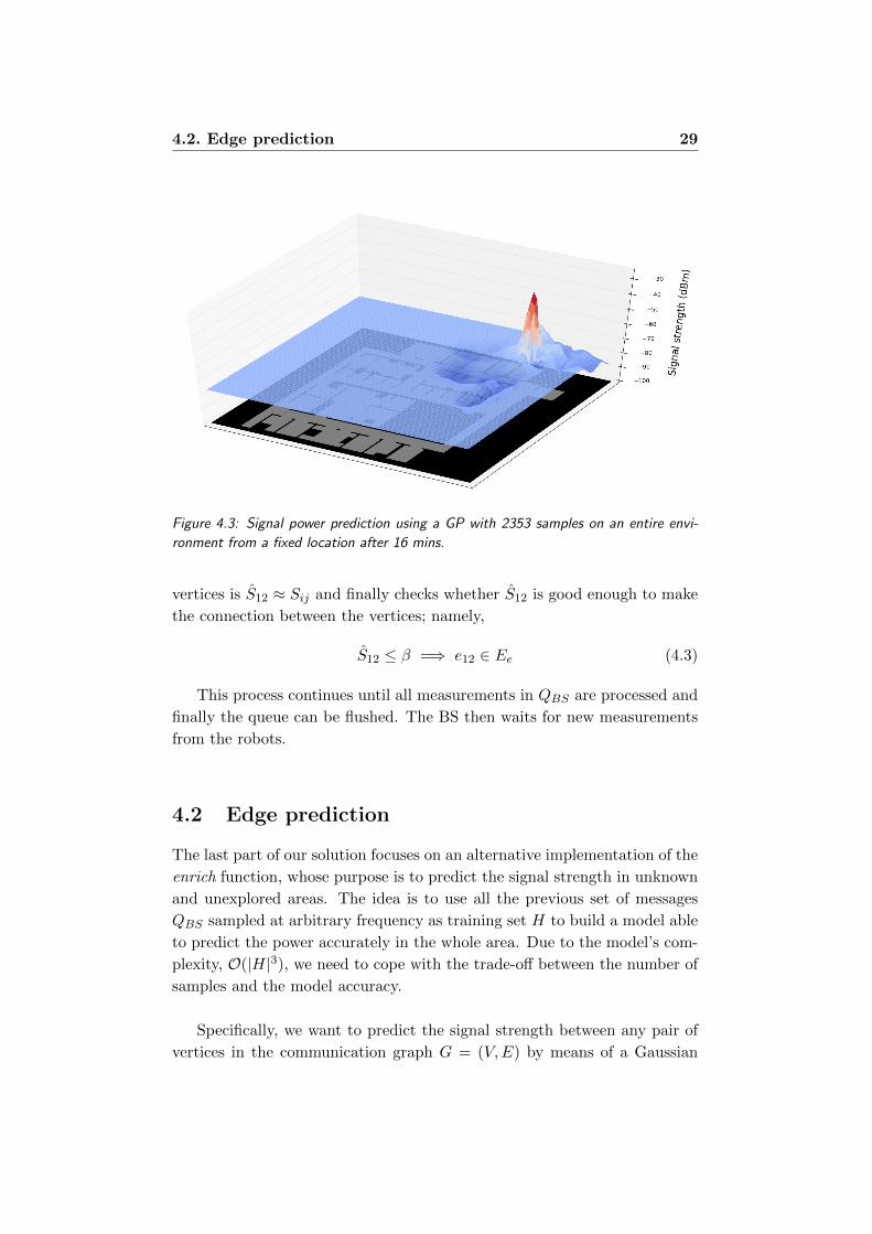
4.3 Signal power prediction using a GP with 2353 samples on an
entire environment from a fixed location after 16 mins. . . . . 29
5.1 Snapshot of filter node sequence. . . . . . . . . . . . . . . . . 36
6.1 Stage window where an office-like environment is displayed
with robots (colored square) and their laser range finder (green
areas). . . . . . . . . . . . . . . . . . . . . . . . . . . . . . . . 40
6.2 Rviz window with environment office. . . . . . . . . . . . . . 41
6.3 Environments used for experiments. . . . . . . . . . . . . . . 42
6.4 TurtleBot equipped with Kinect sensor. . . . . . . . . . . . . 43
6.5 Initial positions of robots in office. . . . . . . . . . . . . . . . 47
6.6 Building a communication map over office with an increasing
number of samples in the training set of the GP (from left to
right, top to bottom). . . . . . . . . . . . . . . . . . . . . . . 48
6.7 Explored area and traveled distance in office. . . . . . . . . . 53
6.8 Communication map with respect to BS position over office
at t = 20 min. . . . . . . . . . . . . . . . . . . . . . . . . . . . 54
6.9 Explored area and traveled distance in cluttered. . . . . . . . 55
6.10 Communication map with respect to BS position over clut-
tered at t = 20 min. . . . . . . . . . . . . . . . . . . . . . . . . 56
6.11 Explored area and traveled distance in openspace. . . . . . . . 58
6.12 Communication map with respect to BS position over openspace
at t = 20 min. . . . . . . . . . . . . . . . . . . . . . . . . . . . 59
VII
6.13 Comparison of explored area and traveled distance in office
under different settings. . . . . . . . . . . . . . . . . . . . . . 60
A.1 Rviz snapshot at time t = 5 min. . . . . . . . . . . . . . . . . 73
A.2 Rviz snapshot at time t = 10 min. . . . . . . . . . . . . . . . 74
A.3 Rviz snapshot at time t = 15 min. . . . . . . . . . . . . . . . 74
A.4 Rviz snapshot at time t = 20 min. . . . . . . . . . . . . . . . 75
A.5 Rviz snapshot at time t = 25 min. . . . . . . . . . . . . . . . 75
A.6 Rviz snapshot at time t = 30 min. . . . . . . . . . . . . . . . 76
B.1 Communication map with 6 samples as training set. . . . . . 77
B.2 Communication map with 657 samples as training set. . . . . 78
B.3 Communication map with 1410 samples as training set. . . . 78
B.4 Communication map with 1944 samples as training set. . . . 79
B.5 Communication map with 2232 samples as training set. . . . 79
B.6 Communication map with 3088 samples as training set. . . . 80
VIII

List of Tables
6.1 Exploration results for office at t = 20 min. . . . . . . . . . . 53
6.2 Added edges in office at t = 20 min. . . . . . . . . . . . . . . 54
6.3 Exploration results for cluttered at t = 20 min. . . . . . . . . 56
6.4 Added edges in cluttered at t = 20 min. . . . . . . . . . . . . 57
6.5 Exploration results for openspace at t = 20 min. . . . . . . . . 57
6.6 Added edges in openspace at t = 20 min. . . . . . . . . . . . . 59
6.7 Exploration results in office at t = 20 min under different
settings. . . . . . . . . . . . . . . . . . . . . . . . . . . . . . . 61
6.8 Added edges in office at t = 20 min under different settings. . 61
IX

X

Chapter 1
Introduction
In multirobot systems, a group of robots coordinate in order to reach a
common goal. Adopting teams of autonomous mobile robots can provide
significant advantages, like improved efficiency, reliability, and robustness,
in accomplishing information-gathering tasks, like exploration, surveillance,
and inspection [1].
One of the most important fields in which multirobot systems are em-
ployed is the exploration of unknown environments. In several applications,
such as map building and search and rescue, robots must efficiently discover
free spaces and obstacles and, at the same time, share operational knowledge
through an ad hoc network. In such scenarios, the process of discovering
unknown features of the environment can be modelled with the following
operations iteratively undertaken by each robot: (i) perceive the surround-
ing environment, (ii) integrate perceived data in a map representing the
environment known so far, (iii) decide the next locations to reach, and (iv)
move to the selected locations [2].
This task requires communication among the members of the team:
robots can share the data they gather only with teammates within a commu-
nication range depending both on their transmission capabilities and on the
environment [3]. The main goal of robots is to move toward the frontiers of
the environment – i.e., the boundaries between mapped and unknown space
– in order to complete the exploration while minimizing the time required.
A base station (BS) – i.e., a fixed entity that allows a human operator to
maintain control over the activity of the robot team – decides which frontiers
robots have to explore, according to a communication model that determines

2 Chapter 1. Introduction
the possibility of communication between any two given points of the envi-
ronment.
In the literature, it is often assumed that robots can always communi-
cate with each other with high-bandwidth [4], [5]. However, such a strong
assumption is not necessarily satisfied in real-life applications and this has
an impact on the performance of the system. Recurrent connectivity con-
straints can provide a good trade-off between situation awareness and explo-
ration efficiency. With recurrent connectivity, robots have to connect with
each other and with the BS each time they gather new information. This
entails that robots can disconnect for arbitrarily long periods, but they must
be able to coordinate in order to report to the base station as soon as new
information is acquired.
Among all the exploration strategies presented in the literature, [2] and
[6] adopt a two-stage approach, which aims at improving computational ef-
ficiency by separating the problem of locations’ selection from that of robot-
location assignments. Planning is decomposed in two stages: (i) an optimal
set of connected locations is computed abstracting away from the robot-
location assignments and (ii) the most efficient assignment of robots to the
locations found in the first stage is computed.
In the strategy briefly described above, the system often needs to possess
knowledge about the possibility of establishing wireless communication links
between arbitrary pairs of locations in order to compute sets of connected
locations, which is represented in a communication map of the environment.
The problem, for a team of robots, is to build it from the measurements
they collect in the environment.
The mainstream approach – also employed in [7] and [8] – assumes such a
map to be given in advance in the form of a graph whose vertices correspond
to physical locations and edges indicate the possibility of communication be-
tween them. The computation of this graph is assumed to happen offline
by means of some link detection mechanism which, given a map of the envi-
ronment, computes which pairs of nodes should be connected with an edge
because communication is possible. As discussed in [9], offline link detec-
tion mechanisms are either too conservative or unreliable and poses the need
for methods that build models of communication capability based on signal
strength measurements gathered on the field.

3
In this context, [10] introduces a formal representation of communication
maps exploiting Gaussian Processes (GPs) [11]. GPs are a tool widely used
in robotics especially in applications involving spatial physical phenomena
that have to be mapped or monitored; see [12], [13], [14]. The work then
tackles the problem for a team of mobile robots to autonomously construct
such maps from on-the-field measurements of WiFi signal strength.
The purpose of the thesis is to improve the performance of an exploring
multirobot system by updating the communication map with new links that
allow robots to explore frontiers more efficiently while maintaining the con-
nection with the BS. More precisely, our work starts from a conservative a
priori model that builds the communication graph of the environment and
implements methods to enrich such graph.
We firstly cope with the problem of exchanging information among the
members of the robot team: the scans of the environment they take while
exploring their assigned frontiers and the signal strength measurements each
pair of robots collect over the environment. We adapt a simulated multi-
robot system, in which all robots and the BS are always assumed to be
able to communicate with each other, to a real context by implementing
a ROS node that routes such information only between robots that are in
communication according to a model based on signal strength, instead of
broadcasting any information over the whole team.
Then, we implement two methods that update the distance-based com-
munication model. The first method is based on actual measurements and
adds links between locations around which robots measure a sufficiently
strong WiFi signal. The second method is based on predicted measures ob-
tained from a Gaussian Process, which exploits the measurements of signal
strength gathered on the field by to estimate signal strength over the whole
environment.
We test the enhanced multirobot system in three different simulated en-
vironments and we evaluate it in terms of explored area and distance traveled
by the robots. Results show that, in general, the new features are actually
able to enrich the communication graph of the environment, and that an en-
riched graph improves the performance of the exploring system. However,
not all the environments benefit in the same measure from our work, due to
their different physical features.

4 Chapter 1. Introduction
Future works in the context of our thesis may follow two main directions.
The first is to generalize the problem and to build a multirobot system that
is more realistic in its components and more adaptable to the features of real
environments; for example, by considering an heterogenous team composi-
tion or a dynamic environment. The second is to develop other algorithms in
order to obtain a further improvement of exploration abilities of the multi-
robot system; for example, by considering multi-team exploration, explicitly
pursuing the communication task, or further enhancing our algorithms.
The thesis has the following structure. Chapter 2 gives a detailed overview
of the state of the art in terms of exploration and coordination strategies and
of communication models, along with a presentation of the communication
maps and the predictive process that generates them. Chapter 3 describes
the problem of multirobot exploration and the optimization of the commu-
nication graph, together with the goals accomplished by this thesis. Chapter
4 presents the solution to the problem describing the polling mechanism im-
plemented in the multirobot system and the two algorithms that enrich the
communication graph. In Chapter 5, the software architecture is presented.
In particular we give a short overview of the ROS framework for multirobot
system programming, before moving to the implementation details of our
mechanism and algorithms. Chapter 6 reports the experimental evaluation
of our work and compares the results in different settings and environments.
Chapter 7 summarizes the purpose and the outcomes of this thesis; it also
proposes some directions for future works.

Chapter 2
State of the art
In this chapter we present the state of the art in the fields of coordinated
exploration strategies and communication models for multirobot systems,
focusing specifically on the assumptions our work is based on. Then we
give an overview of communication maps and of the processes allowing to
generate them in order to achieve a faster exploration.
2.1 Exploration of the physical features of envi-
ronments
Multirobot systems are systems where, typically, a group of robots coordi-
nates themselves to achieve a common goal. One of the most important
fields in which multirobot systems are employed is the exploration of an
unknown environment. Exploration of initially unknown environments is an
online task in which autonomous mobile robots coordinate themselves in or-
der to efficiently discover free spaces and obstacles [15]. Often, they are also
required to communicate their collected data to a base station, which is in a
fixed position of the environment (possibly the starting one for the robots),
where, for example, a human operator can keep track of the progress that
is made [3]. In order to achieve these results the system should possess:
• An exploration strategy, which is used by robots to decide where
they should move. The main goal is to move to the frontiers in order
to complete the exploration of the environment minimizing some kind
of measures like the time required, as shown in [5].
• A coordination strategy, with which the group of robots decide
where every member should be placed to accomplish the exploration

6 Chapter 2. State of the art
mission. This form of coordination is often developed assuming the
possibility of communication with unlimited range and bandwidth.
However, in real world settings, this assumption usually does not hold.
A multirobot exploration system relies on both exploration strategy and
coordination strategy and is affected by the communication constraints en-
forced by the system.
2.1.1 The exploration problem
From a very broad prospective, the exploration problem can be represented
as shown in [16]. Assume to have a two-dimensional environment Env and
assume time is discretized in steps. A set of n robots equipped with a
laser scanner, R = {r1, r2, . . . , rn} is able to move in Env. For any time t,
call pti ⊂ Env the portion of the environment know by robot i. The map,
representing the portion of the environment perceived by robots at time t,
is given by:
M t =⋃
i=0...n
⋃t=0...t
pti (2.1)
The exploration is complete when there is a time t where M t = E. The
problem of an exploration strategy in multirobot systems is to find, at any
time t (or after a given temporal deadline), which frontiers (i.e., the borders
between M t and free space of Env) a robot should reach next, while opti-
mizing a performance measure (such as time required or distance traveled to
complete exploration). The decision on which frontiers to choose and where
each robot goes form the exploration and coordination strategies and they
can be considered the “intelligence” of the system.
A common approach is to use a utility function that typically encodes
benefits and costs of going to different frontiers, as explained in [5], which
can easily be extended for use by multiple robots, like in [17]. Utilities of
individual frontiers may include a factor related to likelihood of communi-
cation success, so robots are less likely to explore areas that take them out
of the team communication range.
Different solutions can be developed to solve the exploration problem
under the assumption of limited communication, but all of them bring same
common challenges to the whole system. Firstly, in real world settings,

2.1. Exploration of the physical features of environments 7
additional constraints can be imposed over the communication of the sys-
tem. For example, a human operator could be interested to receive a video
stream from robots cameras. This scenario can lead to systems in which
all the robots need to build a chain of locally communicating teammates to
relay the video stream from the point of interest, as in [18].
Secondly, robots can predict, using a communication model, when and
where they are able to communicate with other teammates. However, this
prediction could turn out to be wrong and this can have a significant impact
on the performance of the system itself. In order to reduce this degradation,
at the expenses – potentially – of the efficiency of the system in the explo-
ration task, a conservative assumption over the capabilities of the robots to
communicate can be made, as shown in [19].
Thirdly, two robots, at a given time step t, can have different knowledge
of the environment. This requires a map merging algorithm to integrate the
information on the two robots when they reconnect. Moreover, such differ-
ence can lead to degradation of performance if the coordination mechanism
is not carefully implemented.
The integration of data perceived by different agents produces a common
map which, according to [20], can be classified as follows:
• Metric map: it describes the environment showing which areas are
free and which ones are occupied (as an example, by the presence of
an obstacle, such as a wall). There are numerous ways to represent a
metric map: the most used is the grid map, in which the environment
is divided in a set of regular cells, which contain the probability to
encounter an obstacle in the area corresponding to the cell.
• Navigation map: it describes the environment in the form of nav-
igation goals for a robot, which can be specific locations in the envi-
ronment. It is represented with a graph built as the robot explores the
environment, where the vertices represent locations in the free space
and edges are paths between them. A new vertex is placed in the map
whenever the robot has traveled a certain distance from the closest
existing vertex. The final graph serves for planning and autonomous
navigation in the already visited part of the environment.
• Topological map: it describes the environment in terms of a graph
consisting of vertices and edges, which represent rooms in the envi-

8 Chapter 2. State of the art
ronment and their connectivity, respectively. The structure of the
topological graph is built based on the assumption that the transition
between two rooms happens through a door. This allows reasoning on
a human-like qualitative segmentation of an indoor space into distinct
regions.
It is useful to note that all these maps, beside the metric one, built on
the top of the previous ones. For instance, the navigation map is linked with
the metric one, because each vertex of the graph is assigned a position in
metric coordinates, while the topological map can be seen as a more abstract
representation of the navigation graph, where the vertices are grouped by
their position in the environment.
2.1.2 Coordination of robots in communication-restricted en-
vironments
A typical mobile robot used in exploration tasks is usually able to exchange
information with its teammates and possibly with a BS, over a radio chan-
nel, such as WiFi, whose quality degrades with the distance and the presence
of obstacles. The issues of communication can be classified into the connec-
tion requirements imposed from mission objectives, and the communication
model describing the prior knowledge each robot has on its ability to com-
municate with other robots.
The connection requirements to which a multirobot system should com-
ply to achieve the exploration goal can be divided, according to [16], in three
main categories: no connectivity, continuous connectivity and recurrent con-
nectivity.
No connectivity contraints In this case, connections are episodic, not
planned in advance, events which robots can discover only when they actu-
ally happen and exploit to improve decision-making through opportunistic
coordination. In [17], robots coordinate locally with teammates currently
in communication in order to minimize the overlap in the information they
collect when visiting new frontiers. This decision-theoretic framework is
extended in [21] to bias the exploration toward areas that reduces the lo-
calization uncertainty of the robots. The work [22] proposes a distributed

2.1. Exploration of the physical features of environments 9
exploration algorithm and a communication model based exclusively on dis-
tance is exploited to derive a guarantee for the perfect functionality of the
algorithm with respect to the robots’ perception range. In [23], robots com-
pute the expected quality of the signal between a fixed BS and the candidate
target frontiers, and the exploration is biased toward those frontiers where
communication between robots and BS is highly likely. [24] applies a role-
based strategy, which divides robots in explorers of new regions and relays
travelling back and forth to deliver the collected information to the BS,
and extends it with the possibility of arranging rendezvous assuming to be
able to communicate through walls. In [25], the exploration algorithm for
graph-represented environments allows robots to coordinate themselves by
dropping “bookkeeping devices” when visiting graph vertices, whose state
can be read and changed by subsequent visiting robots.
Continuous connectivity In this case, each robot must maintain con-
nection with its teammates (as well as the BS), either in a direct or in a
multihop fashion. This is useful in situations where real-time image stream-
ing must be available to human operators or to ensure a high degree of
coordination. The systems in [19] and [26] leverage on a small set of be-
haviors to perform exploration, with one behavior in charge of regaining
connection with other team members as soon as it is lost. In the former
work, the exploration strategy is tested in scenarios with increasing amount
of prior information about the environment; in the latter work, the explo-
ration strategies are guaranteed to achieve full exploration of an unknown
environment with an architecture that uses few behaviors, messages locally
exchanged between robots, and dropped beacons. [27] devises a centralized
exploration strategy in which a local search method is in charge of guiding
the team: the utility of a configuration for the team is computed in terms
of distances from the closest frontiers.
Recurrent connectivity In this case, robots must regain connection with
teammates according to a particular policy triggered by some kind of events,
such as the discovery of new information about the environment, or simply
striking a timeout. In [8], for an information-gathering mission, the ad-
dressed problems are to find a deployment of relay robots which ensures
global connection and, given the current deployment and the new locations
that agents should reach, to find the redeployment of relay robots which
minimizes their traveling time. In [6], the authors propose a method for
10 Chapter 2. State of the art
multirobot exploration that ensures, besides full connectivity from the fron-
tiers to a BS each time the robots visit a new frontier, a sufficient bandwidth
for the transmission of data on the relay chain. In [28], the behavior of the
robots is regulated by a utility function which considers the amount of in-
formation a robot has not yet delivered to the BS and the estimated amount
of information known by the BS. A parameter allows the mission planner to
specify strategies ranging from an exploration with no returns to the BS to
an exploration ensuring the maximum update frequency at the BS.
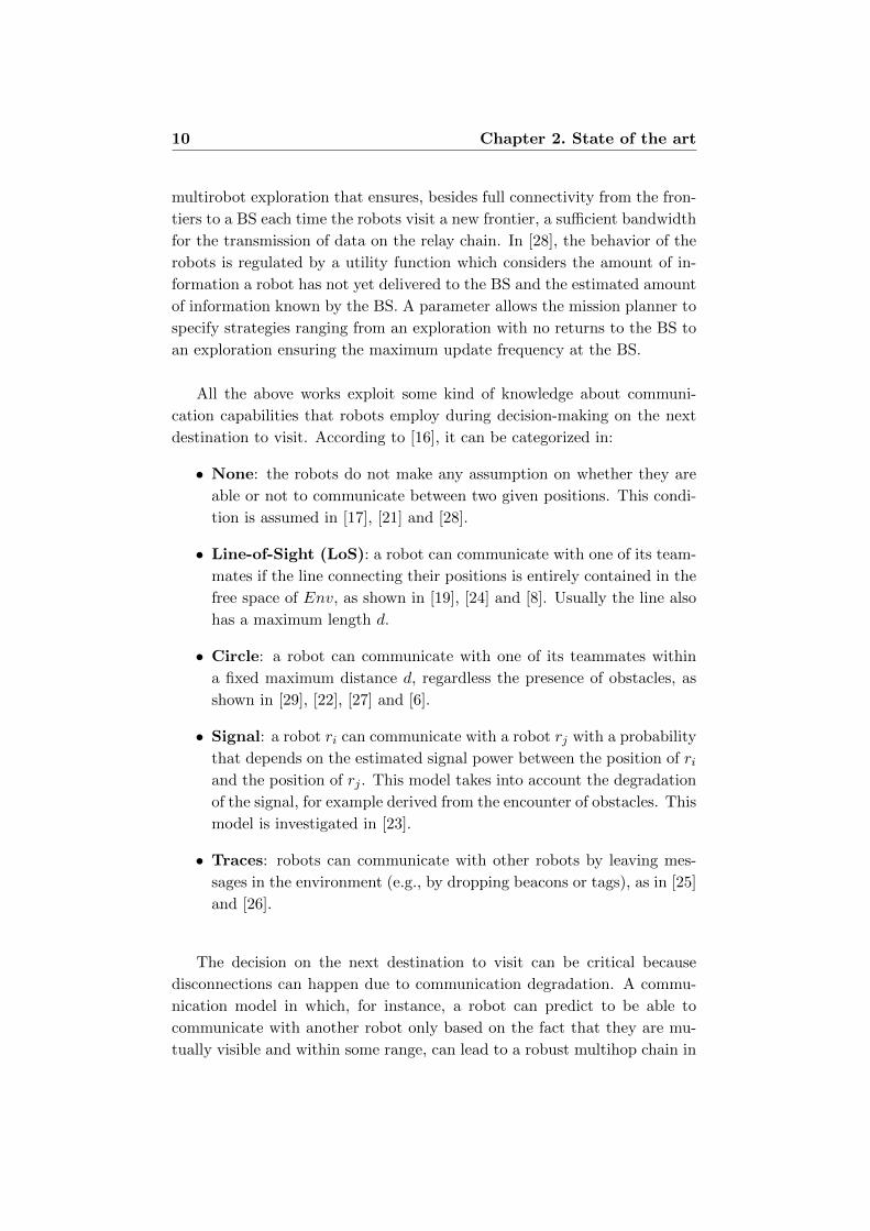
All the above works exploit some kind of knowledge about communi-
cation capabilities that robots employ during decision-making on the next
destination to visit. According to [16], it can be categorized in:
• None: the robots do not make any assumption on whether they are
able or not to communicate between two given positions. This condi-
tion is assumed in [17], [21] and [28].
• Line-of-Sight (LoS): a robot can communicate with one of its team-
mates if the line connecting their positions is entirely contained in the
free space of Env, as shown in [19], [24] and [8]. Usually the line also
has a maximum length d.
• Circle: a robot can communicate with one of its teammates within
a fixed maximum distance d, regardless the presence of obstacles, as
shown in [29], [22], [27] and [6].
• Signal: a robot ri can communicate with a robot rj with a probability
that depends on the estimated signal power between the position of riand the position of rj . This model takes into account the degradation
of the signal, for example derived from the encounter of obstacles. This
model is investigated in [23].
• Traces: robots can communicate with other robots by leaving mes-
sages in the environment (e.g., by dropping beacons or tags), as in [25]
and [26].
The decision on the next destination to visit can be critical because
disconnections can happen due to communication degradation. A commu-
nication model in which, for instance, a robot can predict to be able to
communicate with another robot only based on the fact that they are mu-
tually visible and within some range, can lead to a robust multihop chain in

2.1. Exploration of the physical features of environments 11
case we need a stable video stream between a location of interest and the BS.
2.1.3 Asynchronous exploration under recurrent connectiv-
ity
Among all the possible combinations of exploration strategies and connec-
tion requirements, we focus our attention on a strategy ensuring centralized
asynchronous exploration with recurrent connectivity, that is the one em-
ployed in the course of this thesis. In such circumstances, robots must dis-
cover new information about the environment and, at the same time, share
operational knowledge with a base station through an ad hoc network. The
exploration and coordination strategies must allow the robots to cooperate
with their teammates to form such a network in order to satisfy recurrent
connectivity constraints – that is, data must be shared with the base sta-
tion when making new observations at the assigned locations. Centralized
means that there is a central entity, the BS, acting as a collector of all the
information and as a global planner that decides where to send the robots.
Asynchronous means that it is possible to issue new plans to subgroups of
robots when they are ready to receive them. Readiness is the state in which
robots have reached their goal locations and transmitted all the information
acquired therein. The BS monitors the readiness status of each robot, so
that once a sufficient number of robots becomes ready, the BS issues a new
plan.
In this context, robots not only have to efficiently explore, but also need
to report and share the data they gather by communicating with each other
and with the BS. This entails a critical tradeoff: loose connectivity con-
straints allow robots to explore the environment more efficiently, but reduce
the situational awareness at the BS. On the other hand, strict connectivity
constraints – e.g., requiring the whole team to be always globally connected
– restrict the explored area but increase mission awareness at the BS.
As said before, the recurrent communication model ensures global con-
nectivity only at the deployment locations of the robots, thus enforcing con-
nectivity each time a robot collects new data. New information is gathered
at the robots’ goal locations, and robots can get disconnected for arbitrarily
long periods of time while traveling to them.
Exploration under such and similar constraints are widely covered by the
12 Chapter 2. State of the art
literature. Apart from [2], [30] studies the problem of mobile sensors place-
ment for maximizing the coverage of an unknown area while keeping each
vertex connected to a BS via a multihop mutual-visibility constraint. The
work of [8] tackles the problems of (i) finding a deployment of relay vertices,
which ensures global connectivity between each agent and the BS, and (ii)
given the current deployment and new locations agents should reach, finding
the redeployment that minimizes robots’ traveling time; the former problem
is reduced to the computation of a minimum Steiner tree with the agents’
locations as terminal set, while the latter is solved by using a (generally
sub-optimal) dynamic programming algorithm. [6] proposes an approach
that takes into account bandwidth constraints over the robots relay chain
under the circle communication model and new plans are computed once
the whole network has been formed; the general optimization problem is
split into the sub-problems of explorers placement, relays placement, and
robot path generation. Given a set of candidate locations to be connected,
relays placement is achieved by solving variations of the minimum Steiner
tree problem with minimum number of Steiner points and bounded edge
length [31].
Under recurrent connectivity constraint, [2] proposes two novel asyn-
chronous strategies that work with arbitrary communication models: a sin-
gle strategy based on Integer Linear Program (ILP) for selecting and as-
signing robots to locations, and a two-stage strategy to improve computa-
tional efficiency by separating the problem of locations’ selection from that
of robot-location assignment.
The optimal one-stage approach finds the optimal robots’ deployment
for a set of ready robots by solving a single ILP. The ILP is such that its
optimal solution encodes a deployment that maximizes a weighted combi-
nation of the information gains and traveling costs.
The optimal and approximate two-stage approach was introduced in [32]
and exploits a decomposition into two sub-problems. The first stage is the
optimal configuration problem, which looks for the configuration (i.e., lo-
cations in the environment) that maximizes a utility function defined on
frontiers and that satisfies the recurrent connectivity constraints. The sec-
ond stage is the optimal deployment problem, in which, given the optimal
configuration calculated in the previous stage, the robot-location assignment
that minimizes the traveling costs is computed.

2.2. Mapping communication features 13
This work basically constitutes the exploration strategy that we integrate
in our multirobot system with another task, related to the communication
issue, presented in the next section.
2.2 Mapping communication features
The critical importance of communication in many multirobot information-
gathering tasks requires the availability of reliable signal strength maps.
Such maps can be used to predict the presence of communication links be-
tween different locations of the environment.
Communication is a fundamental activity for multirobot systems. Ex-
changing information is a basic requirement for a team of mobile robots that
need to cooperate in some tasks. Applications like surveillance or search and
rescue heavily rely on sharing knowledge among robots to ensure situation
awareness and to enable informed autonomous decision making during the
mission. The importance of this issue in multirobot applications is being
increasingly recognized as testified by the rich literature on communication-
aware multirobot systems [7], [8].
As said in 2.1.3, deciding “where to go next” is a key problem in many
multirobot settings, usually addressed by optimizing the selection of loca-
tions according to some task-related objective function [33]. Communication
often comes as a further requirement of seeking locations where robots can
exchange data on a wireless connection, either with a fixed base station [6]
or with teammates [34]. Regardless of the application domain, robots often
need to possess knowledge about the possibility of establishing wireless com-
munication links between arbitrary pairs of locations before moving there.
This knowledge is what can be defined a communication map. The problem,
for a team of robots, is to build it from the measurements they collect in
the environment.
2.2.1 Communication maps
A communication map is a function that, for every pair of locations on
a physical map, indicates the signal power strength between those loca-
tions [10].

14 Chapter 2. State of the art
Formally, the construction of a communication map proceeds as follows.
A team of m mobile robots is deployed in a known environment where free
space is denoted with A ⊂ R2 and pi ∈ A is any location that can be occu-
pied by some robots. Robots are assumed to be able to localize themselves
within a common global coordinate system and to be endowed with an omni-
directional transceiver – for example a WiFi adapter – for transmitting and
receiving data with peers over the radio channel within a maximum rangeRc.
The objective is to provide information about the availability of links
between pairs of locations lying in the free space A. A communication map
is defined as a function f : A × A → R≤0 that estimates the true function
f which, for each pair of locations, returns the corresponding radio signal
strength between locations pi and pj defined as the receiving power mea-
sured in dB at location pj with respect to a signal source placed at location
pi. This quantity directly relates to link estimation over radio transmissions:
the closer it gets to zero the more reliable the transmissions from pi to pjand, therefore, the more likely the availability of a high-bandwidth commu-
nication link from pi to pj .
The mainstream approach for building a communication map in mul-
tirobot systems, like the relevant cases of informative path planning and
exploration shown in [7], [32], assumes the communication map to be given
in advance in the form of a prior which can be easily used to construct a
graph whose vertices represent locations and edges are communication links.
The computation of such a graph is assumed to happen offline by means of
some link detection mechanism based on a communication model like those
described in Section 2.1.2. Such link detection mechanisms use the map of
the environment to decide whether communication is possible between two
locations and add edges to the graph.
As discussed in [9], one important limit of such methods is that robots’
capability of communicating over wireless channels is heavily influenced by
the physical features of the environment that are not stored as information
in the graph (e.g., the density of obstacles or the presence of interferences).
This makes offline link detection mechanisms either too conservative (e.g.,
Circle, Line-of-Sight), or unreliable (e.g., wall propagation model [35]) and
poses the need for methods that build models of communication capability
based on actual signal strength measurements gathered on the field. An ex-
ample is in [36], which aims at deploying a team of networked robots into an
environment for which no accurate radio signal propagation model exists:
2.2. Mapping communication features 15
the mobile robots must autonomously build a map of the signal strength
and localize the base station, which is transmitting from an unknown loca-
tion, by performing online estimation and mapping of received radio signal
strength.
The challenge, for a multirobot system, is to build autonomously a com-
munication map from on-the-field measurements of signal strength, without
any a priori knowledge.
We investigate an approach that employs Gaussian Processes (GPs),
which allows a probabilistically sound way to incorporate noisy measure-
ments from an unknown process (i.e., measurements of signal strength taken
by the team of robots in the environment) and then to make predictions on
the process at unknown states (i.e., predict the signal strength between lo-
cations where measurements have not been collected yet) [36]. Indeed, this
is the approach used in the development of our thesis.
2.2.2 Gaussian Processes
A Gaussian Process is a set of random variables where each finite subgroup
follows a Gaussian multi-variate distribution [11]; as such, the process is
fully specified by a mean function and a covariance function for any given
couple of locations. This process represents a non-parametric method allow-
ing to model physical phenomena with strong spatial variations. Its main
advantage with respect to other techniques is the ability to generate likeli-
hoods at locations for which no data are available, in a statistically sound
way.
There are several ways to construct a GP; the most common approach
is the one described in [11]. Let Y = [y1, y2, . . . , yq]T be the set of the
q measurements collected over the environment by the robot team, X =
[x1, x2, . . . , xq]T the set of corresponding locations from where they have
been collected and yi = f(xi) + ε the noisy process that generates the sam-
ples of the training set, where ε ∼ N (0, σ2n) is the additive sensing error with
null mean and known variance σ2n.
A Gaussian Process estimates posterior distributions over functions f
from training data. A key idea underlying GPs is the requirement that the
function values at different points are correlated, where the covariance be-

16 Chapter 2. State of the art
tween two function values, f(x) and f(x′), depends on the input values, x
and x′. This dependency can be specified via an arbitrary covariance func-
tion, or kernel, k(x, x′).
The most widely used kernel is the squared exponential – or Gaussian –
whose parameters are the signal variance σ2f and length scale l2 that deter-
mines how strongly points correlate:
k(x, x′) = σ2f exp
(− 1
2l2|x− x′|2
)(2.2)
This clearly shows that the covariance between function values decreases
with the distance between their corresponding input values.
For an entire set of input values X, the covariance over the corresponding
observations Y becomes:
cov(Y) = K(X,X) + σ2nIq (2.3)
where K is the n×n covariance matrix of the input values and Iq is the q×qidentity matrix. Such equation represents a prior over functions: for any set
of values X, one can generate the matrix K and then sample a set of corre-
sponding targets Y that have the desired covariance. Indeed, more relevant
is the posterior distribution over functions given training data X,Y, which
allows to predict the function value at an arbitrary point x?, conditioned on
training data X,Y.
The GP is then fully specified by the parameter vector θ = [σ2f , l
2, σ2n]T
and is a zero-mean process. This means that, when far enough from the
access point, all predictions should tend to zero.
The parameters l and σf , which model, respectively, the length scale of
variation and the amplitude of the variance, control the shape of the co-
variance function, and thus together with the noise variance σ2n affect the
behavior of the GP.
As shown in [37], it is possible to learn these parameters based on the
training data X,Y using hyperparameter estimation. Given the parameter
vector θ, its estimation can be computed by maximizing the observations
log-likelihood θ? = arg maxθ log p(Y|X, θ) where:
log p(Y|X, θ) = −1
2
(YT cov(Y)−1Y − log |cov(Y)| − n log 2π
)(2.4)

2.2. Mapping communication features 17
The obtained parameters can then be used to calculate an estimate of
the signal strength in unobserved regions by evaluating the posterior. Called
W = [w1, w2, . . . , wq]T a set of arbitrary location pairs for which a signal
strength estimate is requested, it holds that:
p(f(W)|X,Y) ∼ N (µW,ΣW) (2.5)
where µW = K(W,X)cov(Y)−1Y is the mean vector and ΣW = K(W,W)−K(W,X)cov(Y)−1K(W,X)T is the covariance matrix. The main diagonal
of ΣW represents the predictive variance and is used to measure the uncer-
tainty of estimates in W.
GPs are a widely used tool in robotics especially in applications involving
spatial physical phenomena that have to be mapped or monitored [12], [14].
The following properties, listed in [37], in fact, make them ideally suited for
modelling signal strength measurements:
• Continuous locations: GPs do not require a discretized represen-
tation of an environment, or the collection of calibration data at pre-
specified locations. They are able to predict signal strength measure-
ments at arbitrary locations.
• Arbitrary likelihood models: GPs are non-parametric regression
models and thereby able to approximate an extremely wide range of
non-linear signal propagation models.
• Correct uncertainty handling: In contrast to other regression
models, GPs provide uncertainty estimates for predictions at any set
of locations. This uncertainty takes into account the local density of
calibration data and the noise of the data points.
• Consistent parameter estimation: The parameters of GPs can
be learned from the calibration data via hyperparameter estimation.
These parameters include the spatial correlation between measure-
ments and the measurement noise.
Because of their versatility, GPs are used in a variety of fields: sensor
networks [38], data visualization [39], computer animation [40], mapping gas
dispersal [41] and sensor-centric localization for mobile robots [42]. The abil-
ity of GP to provide the maximum likelihood estimate is exploited in [36],

18 Chapter 2. State of the art
which performs online mapping of received radio signal strength with mobile
robots to localize the source of the radio signal by predicting the received
signal strength with confidence bounds in regions of the environment that
have not been explored. In [9] the WiFi SLAM problem is solved using a
GP to reconstruct the topological connectivity graph from a signal strength
sequence which can be used to perform efficient localization. In [13] a de-
centralized multirobot exploration is carried on by modelling the spatial
correlation of measurements of a terrain profile to reduce the number of
measurements needed.
In [10], a method for a team of autonomous mobile robots is proposed
to build communication maps by integrating in a GP the signal strength
measurements gathered on the field and devises a formalism to represent
communication maps in robot-to-robot communication settings and some
online sensing strategies that robots can use to coordinate and optimize
data acquisition. Formally, the approach is to maintain the communication
map f as a posterior distribution fitted over a set of noisy observations made
by robots which explore and coordinate in the environment to gather signal
strength measurements. The GP, in fact, provides a mechanism to integrate
noisy readings performed in the environment into a posterior distribution of
the signal strength that can be used to obtain link estimates with quantified
uncertainty.
Chapter 3
Problem definition
In this Chapter we present a formal definition of the problem addressed
in this work. We start by defining the research area. Then, we list the
assumptions underlying our work and set the thesis goals.
3.1 Multirobot exploration
As already stated in Chapter 2, one of the most important fields in which
multirobot systems are employed is the exploration task in an unknown en-
vironment. Multirobot systems need exploration and coordination in order
to be able to manage the exploration task assigned. The two categories
of strategy (namely, exploration and coordination) can have different prac-
tical implementations, but they essentially leverage information about the
environment in order to be as fast as possible in fully discovering the envi-
ronment, while trying to travel the less distance as possible in order to save
energy.
The difficulty in finding a good solution increases if we consider that
the whole system has to comply with a communication model that can be
updated during the exploration mission.
In the adopted solution, robots take measures about signal power strength
together with those about the presence of obstacles and free space, which
usually characterize exploration, in order to build and update a communi-
cation map that informs the exploration decisions.

20 Chapter 3. Problem definition
3.2 Problem and goals
The work we propose focuses on the problem of building a multirobot system
which is able to explore an unknown environment using a fixed exploration
strategy and different incremental methods to enrich the communication
graph by predicting connectivity in unknown and unexplored areas. We aim
at identifying new links in the communication graph built by the BS in order
to be more efficient even if the exploration algorithm remains unchanged.
Before explaining in a more rigorous and detailed way the formulation of
the problem, we are going to present some important assumptions we make
in this work.
3.2.1 Assumptions
Environments The first important set of assumptions we have to make
is about the environment. In this work, we consider arbitrary environments,
including both indoor and outdoor, denoted by Env. These environments
can have different shapes and different layouts. The interior points of the
environment can belong to obstacle of arbitrary shape whose set is denoted
by Envo, or can belong to the free space, denoted by Envf = Env \ Envo.Moreover, we assume that these environments are static during the explo-
ration task, meaning that they are not changing during exploration. Lastly,
we assume these environments to two-dimensional and formed of a single
floor, Env ⊂ R2. However, extensions of the following method to three-
dimensional environments is straightforward.
Robots A second set of assumptions has to be made over the robots. In
this work we consider to have a multirobot system in which a team of mobile
robots R = {r1, r2, . . . , rn} are exploring an initially unknown environment.
Moreover we have another agent, the base station, which plays the role of a
supervising control center, deployed in Env at a fixed location. The BS is
incapable of moving and it needs to receive updates about the mission status
and the exploration task, so it must be able to communicate with the robots.
The robots are able to move around in the free space of the environment
and they are equipped with a finite-range sensors able to perceive the sur-
rounding free space and outer boundaries of obstacles, such as laser scanners,
which are the input to the SLAM (simultaneous localisation and mapping)
3.2. Problem and goals 21
module [43]. The BS instead does not have any sensor and it relies only on
the robots to perceive the environment. We assume the SLAM module to
provide reasonably accurate localisation. This can be considered a realis-
tic assumption, because recent approaches, such as those purely basing on
scan-matching, as it is explained in [44], or on particle filters (like in [45]),
are considered robust when dealing with noisy data. This assumption gives
us the possibility to focus our work specifically on the identification of new
links, instead of dealing with noisy data that require filtering.
Furthermore, the BS and the robots maintain and update a map rep-
resenting the portion of environment discovered so far, represented as an
occupancy grid which is updated each time new information is sent by the
robots.
Communication A last set of assumptions can be made about the com-
munication between robots (including the BS). All the robots (and con-
sequently the BS) are equipped with RF transceivers (e.g., WiFi). These
transceivers are typically assumed to have an unlimited bandwidth channel,
when signal strength is good, that can be used by the robots to exchange
information. In the literature, it has been shown that this assumption can
hold even in real setting. For instance, in [32], the authors show that this
assumption does not affect the performance of a real multirobot system.
The transceivers have a maximum communication radius d which can vary
according to the environment.
We assume, moreover, the communication to be perfect. This means
that if the model guarantees that two agents can communicate, they are
actually able to do it and there is no loss of information over the channel,
meaning that all the information sent is always delivered.
Exploration For simplicity, as shown in [2], we assume that time evolves
in discrete steps t ∈ {1, 2, . . . , T}, where T denotes the last step of the ex-
ploration mission. Upon the grid-based map known at a generic time step
t, the BS is able to construct a graph-based representation of the environ-
ment Gt = (V t, Et), where vertices in V t encode some discretization of the
portion of Envf known so far. Each vertex v ∈ V t is associated with a
candidate robots’ goal location, except for the vertex b which denotes the
fixed position of BS. A set F t ⊆ V t \ {b} denotes the exploration frontiers,

22 Chapter 3. Problem definition
that is, vertices corresponding to locations of Envf lying on the boundary
between explored and unexplored portions of Env.
As customarily done in robotic exploration, each vertex v ∈ V t is asso-
ciated with a numerical value g(v) representing the (expected) information
gain obtainable by taking a perception from v. Typically, the information
gain is 0 when v /∈ F t, and proportional to the new area expected to be seen
from v, otherwise. Each pair of vertices i, j ∈ V t is associated with a value
d(i, j), representing the distance between them as known by the BS and the
robots. The edge set Et encodes the communication features of the environ-
ment. In particular, this set is determined by link-detection mechanisms in
charge of recognizing the availability of a communication link between any
two known vertices. In order to define the ability to communicate between
two vertices i,j ∈ V t we define an edge matrix M tij as a binary matrix. The
presence of an edge eij in the communication graph Gt is equivalent to a 1
in the edge matrix M tij , and vice versa.
The exploration process terminates once the environment has been en-
tirely mapped or after a predefined deadline is reached.
3.2.2 Communication graph optimization
The aim of this work, as already mentioned before, is to build a system
under recurrent connectivity constraint [32] that is able to add previously
absent edges – due to lack of knowledge of the environment – to the com-
munication graph G and, implicitly, 1s to the edge matrix M .
In order to perform this task, instead of using a dedicated team to build
a communication model of the world as shown in [10], we decide to use a
single team committed to explore the environment, build a communication
map as a byproduct and simultaneously gather additional data.
For this purpose, robots do not just scan and acquire obstacles infor-
mation about the environment but they also constantly measure the signal
power strength Sij(pi, pj), where pi and pj are the location of the robots
where measurements have been taken. These measurements are eventually
sent to the BS which stores them asynchronously in a queue Qt.
Within the framework described above, the exploration evolves as fol-
3.2. Problem and goals 23
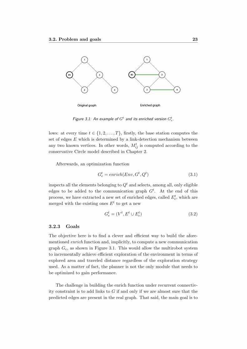
Figure 3.1: An example of Gt and its enriched version Gte.
lows: at every time t ∈ {1, 2, . . . , T}, firstly, the base station computes the
set of edges E which is determined by a link-detection mechanism between
any two known vertices. In other words, M tij is computed according to the
conservative Circle model described in Chapter 2.
Afterwards, an optimization function
Gte = enrich(Env,Gt, Qt) (3.1)
inspects all the elements belonging to Qt and selects, among all, only eligible
edges to be added to the communication graph Gt. At the end of this
process, we have extracted a new set of enriched edges, called Ete, which are
merged with the existing ones Et to get a new
Gte = (V t, Et ∪ Ete) (3.2)
3.2.3 Goals
The objective here is to find a clever and efficient way to build the afore-
mentioned enrich function and, implicitly, to compute a new communication
graph Ge, as shown in Figure 3.1. This would allow the multirobot system
to incrementally achieve efficient exploration of the environment in terms of
explored area and traveled distance regardless of the exploration strategy
used. As a matter of fact, the planner is not the only module that needs to
be optimized to gain performance.
The challenge in building the enrich function under recurrent connectiv-
ity constraint is to add links to G if and only if we are almost sure that the
predicted edges are present in the real graph. That said, the main goal is to

24 Chapter 3. Problem definition
decide when an edge should be added to the communication graph. More
precisely, if we carelessly add a link at the very beginning, we are not sure
about it, and it can cause a problem during the exploration. On the other
hand, if we add it on the later stages, we may lose all the benefits deriving
from it.

Chapter 4
Problem solution
In this Chapter we present the solution elaborated to the problem formulated
in previous chapter. We start by presenting a logical view of the solution
implemented given an instance of the original problem.
We extend the two-stage approach proposed in [2] by adding a strategy
to enrich the communication graph G. This strategy does not instantiate
a hierarchy in the team of the robots, considering all of them as explorers.
However, some agents, even if they were all initially considered explorers, be-
gin to act as dedicated relays during the exploration when they meet other
teammates. Furthermore, they often behave like a chain of relays at the
later stages of exploration to preserve the connection with the base station
as shown in Figure 4.1.
In Chapter 3, we provided a formal definition of the graph enrichment
problem and of the goals of our research along with the main modules needed
to accomplish it. In this chapter we present our solution introducing two
different strategies that can work together or standalone. Though, before
analyzing them, we need to focus on how we gather information from the
environment in terms of signal strength between two physical points. To do
so, at first, we implement a polling mechanism which is the basic requirement
for accomplishing our goal.
Polling mechanism
As mentioned above, since we do not want to penalize the time required to
explore an environment, we decide not to spend dedicated robots to collect
information about signal strength: all the robots act in the very same way.

26 Chapter 4. Problem solution
BS
1
2
3
t = 1
BS
1
2
3
t = 2
BS
1
2
3
t = 3
packet to forward
Figure 4.1: Example of relay mechanism from robot 3 to BS.
The BS orchestrates the exploration by sending robots to the frontiers as
reported in [2] to explore a new portion of the map.
In order to make a better and smarter plan and to take advantage of the
time spent to go from the starting point to the assigned goal, in addition to
collecting the information strictly necessary to accomplish the exploration
goal, robots poll each other to acquire additional data regarding the signal
power strength at any selected steps t ∈ {1, 2, . . . , T}.
This knowledge is represented as a tuple q of robot’s coordinates and the
signal power strength between the two. Specifically,
q = 〈xi, yi, xj , yj , Sij〉 (4.1)
that is, robot ri in position (xi, yi) measured the signal power strength Sijwith rj in position (xj , yj). During the navigation, each robot i stores these
tuples in an internal queue Qi and, by means of a relay mechanism, it sends
them back to the BS, eventually flushes the internal queue.
4.1 Edge addition
As stated in Section 3.2.2, enrich is a function that outputs a communica-
tion graph used by the BS to make a new deployment. We propose a first
implementation of the aforementioned enrich function called edge addition

4.1. Edge addition 27
Figure 4.2: Example of three cases of edge addition exploiting polling sample generated
by robots during the navigation with α = 10 m and β = −93 dB.
which aims at improving the communication graph G using an efficient ap-
proach.
The idea behind edge addition is to consider signal strengths measure-
ments of locations near to two arbitrary known vertices of the current com-
munication graph. Clearly, this is an approximation for adding new links to
the communication graph; however this is a valid approximation because it
represents a real communication between robots.
To implement this behavior, we define two parameters, namely α and β,
fixed at the beginning of the exploration. The parameter α represents the
maximum distance between a communication vertex and an actual location
where robots took signal strength measurements, to decide whether the cor-
responding signal strength can be used for edge addition. The parameter β
represents the power strength threshold used to choose whether an edge is
qualified or not to be added to the enriched graph Ge.
The first step of the algorithm (refer to Algorithm 1) focuses on vertex
selection. Given a generic message q = 〈xi, yi, xj , yj , Sij〉 from the queue
QBS , we define pi = (xi, yi) and pj = (xj , yj) as the positions of robot riand rj , respectively.
In order to select the vertices, we iteratively try to match the robot’s po-
sition pi to an existing vertex of the graph v1 ∈ V at position (v1x , v1y). To

28 Chapter 4. Problem solution
Algorithm 1 Edge addition algorithm
procedure edge-addition(Env, G, Q)
for all q ∈ Q do
if qS12 ≤ β then . We discard the message
continue
5:
vertices1 = ∅vertices2 = ∅for all v ∈ G.V do
distance1 = euclideanDistance(vx, qx1 , vy, qy1)
10: inLineOfSight1 = lineOfSight(Env, vx, qx1 , vy, qy1)
distance2 = euclideanDistance(vx, qx2 , vy, qy2)
inLineOfSight2 = lineOfSight(Env, vx, qx2 , vy, qy2)
if distance1 ≤ α and inLineOfSight1 then
15: vertices1.push(v)
if distance2 ≤ α and inLineOfSight2 then
vertices2.push(v)
for all v1 ∈ vertices1 do
20: for all v2 ∈ vertices2 do
if (v1 6= v2 and (v1, v2) /∈ G.E) then . New edge found
G.E.push((v1, v2))
choose which vertex to select, we rely on the Line-of-Sight communication
model illustrated in Section 2.1.2 with maximum distance α. In this way,
the approximation is close to the actual measurements, as obstacles, such as
walls, could greatly affect the signal strength even when two locations are
very close. A similar mechanism is in place for matching robot’s position pjto v2.
We define a binary function LoS : (R2 × R2) → {true, false}, and
euclideanDistance : (R2 × R2)→ R. As represented in Figure 4.2, an edge
between vertices v1 and v2 is added if and only if the following conditions
hold:
LoS(v1, pi) ∧ euclideanDistance(v1, pi) ≤ α ∧LoS(v2, pj) ∧ euclideanDistance(v2, pj) ≤ α
(4.2)
Furthermore, we can assume that the signal strength between the two
4.2. Edge prediction 29
Figure 4.3: Signal power prediction using a GP with 2353 samples on an entire envi-
ronment from a fixed location after 16 mins.
vertices is S12 ≈ Sij and finally checks whether S12 is good enough to make
the connection between the vertices; namely,
S12 ≤ β =⇒ e12 ∈ Ee (4.3)
This process continues until all measurements in QBS are processed and
finally the queue can be flushed. The BS then waits for new measurements
from the robots.
4.2 Edge prediction
The last part of our solution focuses on an alternative implementation of the
enrich function, whose purpose is to predict the signal strength in unknown
and unexplored areas. The idea is to use all the previous set of messages
QBS sampled at arbitrary frequency as training set H to build a model able
to predict the power accurately in the whole area. Due to the model’s com-
plexity, O(|H|3), we need to cope with the trade-off between the number of
samples and the model accuracy.
Specifically, we want to predict the signal strength between any pair of
vertices in the communication graph G = (V,E) by means of a Gaussian

30 Chapter 4. Problem solution
Algorithm 2 Edge prediction algorithm
procedure edge-prediction(G, Q)
X = [Qx1 , Qy1 , Qx2 , Qy2 ] . Robot’s locations
Y = [QS12 ] . Corresponding robot’s measurements
5: gp = new GaussianProcessService()
gp.addTrainingData(X, Y )
W = ∅for all v1 ∈ G.V do
10: for all v2 ∈ G.V do
W .push([v1x , v1y , v2x , v2y ])
predictions, variances = gp.predict(W )
for all p ∈ predictions, v ∈ variances do
15: if p− 2 ∗√v2 > γ then . New edge found
G.E.push((v1, v2))
Process introduced in Section 2.2.2.
As such, we define the following variables: i) X is a matrix that contains
all locations where robots measured the signal strength (e.g., (xi, yi, xj , yj) =
(0, 0, 5, 8) ); ii) Y are the measurements taken at locations X; iii) W is a
matrix composed by all positions where to predict the physical process val-
ues; iv) a parameter γ fixed at the beginning of the exploration represents
the threshold signal strength used to choose whether an edge is qualified or
not to be added to Ge (similarly to the parameter β used in Section 4.1).
We propose an algorithm (refer to Algorithm 2) which takes as input
the current communication graph G, that can be initialized according to [2],
and the queue Q from which we extract the set of locations X and their
corresponding measurements Y and outputs the new enriched graph Ge. In
other terms, given Y and X, we can predict the target values Z = f(W )
for the corresponding W . The elements in H are distributed according to
p(Z|W,X, Y ) = N(µW ,∑
W ) as already described in Section 2.2.2.
Firstly, we use measurements X and Y to learn the model parameters
that represent our data. The better the model, the better the prediction of
the connection between vertices in the communication graph. In a Gaussian

4.3. Combining edge addition and prediction 31
Process, learning the model is equivalent to learn the optimal hyperparam-
eters that characterize the covariance function.
Secondly, we select the set of positions W as the combination of all the
vertices V in the graph and we predict the vector of means µW and the
covariance matrix∑
W in positions of W using the GP model learned pre-
viously. Figure 4.3 shows an example of such prediction.
Thirdly, we look for prediction with low variance, in order to be sure
that the edge really exists in the real communication graph. Let Z12 be the
prediction and δ212 the variance for a pair of vertices v1, v2 ∈ V ; we add an
edge to the communication graph according to:
Z12 − 2 ∗√δ2
12 > γ =⇒ e12 ∈ Ee (4.4)
4.3 Combining edge addition and prediction
In the previous sections we illustrated two methods to improve the commu-
nication graph separately. In Chapter 6, we present experimental results
and we highlight in a very detailed way their advantages and disadvantages.
In principle, we can gain further improvements by using them one after
the other. We can simply parallelize edge addition and edge prediction to get
the best from them. In particular, we start from a communication graph G
created using the Circle model and we add edges by means of edge addition.
As a result, we get a new communication graph Ge1 which is further im-
proved with edge prediction obtaining the final communication graph Ge2 .

32 Chapter 4. Problem solution

Chapter 5
Implementation
In this Chapter we present the architecture of the system, in terms of mod-
ules we have implemented for our research. We start by briefly describing
ROS (http://www.ros.org), the robotics middleware in which we imple-
mented and simulated our algorithms. Then, we overview the main modules
implemented to enable the enrichment functionality within a multirobot ex-
ploration system subject to communication constraints.
5.1 ROS
Robot Operating System is an open-source, meta-operating system for robots
[46]. It provides features such as hardware abstraction, low-level device
control, implementation of commonly-used functionalities, message-passing
between processes, and package management. It also provides tools and
libraries for obtaining, building, writing, and running code across multiple
computers.
The first ROS concept is the Computation Graph. It is a peer-to-peer
network of ROS processes that are processing data together. The basic
Computation Graph concepts of ROS are nodes, Master, Parameter Server,
messages, services, topics, and bags, all of which provide data to the Com-
putation Graph in different ways. We describe only the ones required to
understand the following sections.
• Nodes: nodes are processes that perform computation. ROS is de-
signed to be modular at a fine-grained scale; a robot control system
usually comprises many nodes. For example, one node controls a laser

34 Chapter 5. Implementation
range-finder, one node controls the wheel motors, one node performs
localization, one node performs path planning, one node provides a
graphical view of the system, and so on. A ROS node is written with
the use of a ROS client library, such as roscpp or rospy.
• Messages: nodes communicate with each other by passing messages.
A message is simply a data structure, comprising typed fields. Stan-
dard primitive types (integer, floating point, boolean, etc.) are sup-
ported, as are arrays of primitive types. Messages can include arbi-
trarily nested structures and arrays (similarly to C structs).
• Topics: messages are routed via a transport system that employs pub-
lish/subscribe semantics. A node sends out a message by publishing it
to a given topic. The topic is a name that usually identifies the content
of the message. A node that is interested in a certain kind of data will
subscribe to the appropriate topic. There may be multiple concurrent
publishers and subscribers for a single topic, and a single node may
publish and/or subscribe to multiple topics. In general, publishers
and subscribers are not aware of each others’ existence. The idea is to
decouple the production of information from its consumption. From
a logical point of view, one can think of a topic as a strongly typed
message bus; each bus has a name and anyone can connect to the bus
to send or receive messages as long as they are the right type.
• Services: the publish/subscribe model is a very flexible communica-
tion paradigm, but its many-to-many, one-way transport is not ap-
propriate for request/reply interactions, which are often required in
a distributed system. Request/reply is done via services, which are
defined by a pair of message structures: one for the request and one
for the reply. A provider node offers a service under a name and a
client uses the service by sending the request message and awaiting
the reply. ROS client libraries generally present this interaction to the
programmer as if they were a remote procedure call.
5.2 Communication and filter nodes
Before presenting the main modules we developed, we move the attention
to an important observation regarding the connectivity constraint during
the navigation. We started our implementation from a multirobot system
which, when simulated, allowed any robots (and the BS) to communicate
with each other at all times. In order to make it realistic as well as efficient,

5.2. Communication and filter nodes 35
we design and build a communication node and a filter node.
5.2.1 Communication node
The communication node a central, unique node, connected with all the
agents, as well as the BS, in charge of maintaining a binary connectivity
matrix C along with the estimated signal power strength matrix S. The
communication node follows the publish/subscribe pattern, exposing two
intuitive routine:
• Subscribe robot positions: at every iteration each robot publish
its location in the environment which is stored internally by the com-
munication node.
• Publish matrices: it computes and publishes the connectivity ma-
trix along with the signal power strength matrix. To do that, the
communication node firstly calculates the signal power strength ma-
trix S ∈ RNxN
S =
s11 s12 . . . s1N
s21 s22 . . . s2N...
.... . .
...
sN1 sN2 . . . sNN
(5.1)
according to equation 6.1, and finally generates the multihop connec-
tivity matrix C ∈ {0, 1}NxN . Given Sij , the corresponding Cij = 1 if
Sij is greater than a fixed threshold called Power cutoff, for instance:
C =
1 1 . . . 0
1 1 . . . 1...
.... . .
...
0 1 . . . 1
(5.2)
5.2.2 Filter node
This second component allows agents to exchange packets (which can be of
any type: portion of map, meta information, etc. . . ) if and only if they are
actually connected with each another. To establish whether two robots riand rj are in communication we rely on the communication node introduced
above.
We define the following variables: i) i, the robot we take in consider-
ation; ii) N the number of robots; and iii) a vector Q of length N whose
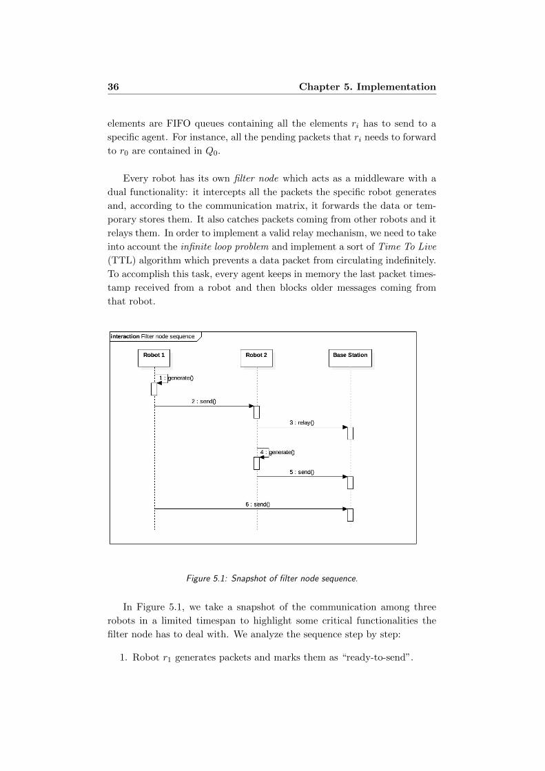
36 Chapter 5. Implementation
elements are FIFO queues containing all the elements ri has to send to a
specific agent. For instance, all the pending packets that ri needs to forward
to r0 are contained in Q0.
Every robot has its own filter node which acts as a middleware with a
dual functionality: it intercepts all the packets the specific robot generates
and, according to the communication matrix, it forwards the data or tem-
porary stores them. It also catches packets coming from other robots and it
relays them. In order to implement a valid relay mechanism, we need to take
into account the infinite loop problem and implement a sort of Time To Live
(TTL) algorithm which prevents a data packet from circulating indefinitely.
To accomplish this task, every agent keeps in memory the last packet times-
tamp received from a robot and then blocks older messages coming from
that robot.
Figure 5.1: Snapshot of filter node sequence.
In Figure 5.1, we take a snapshot of the communication among three
robots in a limited timespan to highlight some critical functionalities the
filter node has to deal with. We analyze the sequence step by step:
1. Robot r1 generates packets and marks them as “ready-to-send”.

5.3. Enrich strategy 37
2. At time step t = 2, ri sends the packets to all the teammates that are
in communication with it according to the communication matrix.
3. Unlike the BS, r2 receives properly the data and relays them to all the
agents it is connected to. At this point, even tough r1 is not directly
connected to the BS, the packet generated at t = 1 reached the BS.
4. Robot r2 makes a similar operation to what done in t = 1 and t = 2
by r1.
5. Eventually, r1 forwards to the BS the packet generated previously.
Since the base station already received this information by means of
r2, it discards the packet.
The filter node logic remains the same even for future implementations
on real robots, although the mechanism through which we detect whether
two robots are in communication will change.
5.3 Enrich strategy
Now that we have a full understanding of the communication modules, we
can describe the functions we built to accomplish our goal. Both the func-
tions edge addition and edge prediction are written in C++ and built inside
the BS planner which is responsible for issuing a new deployment.
5.3.1 Edge addition
As we stated in the previous chapter, edge addition is based only on the
data Q collected by the robots during the navigation. To compute the new
communication graph G we first iterate over the samples in Q, and we imme-
diately discard those samples which power is lower than the fixed threshold
β.
Afterwards, for each message q ∈ Q, we define two sets, namely vertices1
and vertices2, in which we push iteratively the vertices matching our con-
ditions. Then, we cycle over all the existing vertices V of the graph and
we try to associate the position p1 and p2 to the current node v based on
Line-of-Sight communication strategy, populating the two sets vertices1 and

38 Chapter 5. Implementation
vertices2, respectively. At the end of this process, we have two list of ver-
tices corresponding to that specific message q and by combining the two
sets we get a new set of edges that we add to communication graph G. This
process is repeated until we analyze all the messages in Q.
5.3.2 Edge prediction
To accomplish the goal of prediction we design and build an isolated service
instead of the usual publish/subscribe because it is more appropriate for
request/reply interactions.
To implement this service, we rely on a python ROS node with GPy ex-
tensively used in [10]. In order to reuse most of the code already available,
we extended the original node such that it could expose three methods: ad-
dTrainingData, train and predict to which a generic node can make requests.
Moreover, it has an internal training set H which is built based on the data
it receives every time addTrainingData is called. T is an incremental set
and it is used in the learning phase to train the model.
Even tough the service exposes a method to train the model, due to its
complexity and the time required to train the model which grows with the
number of samples – i.e., O(|H|3) – we decided to adopt an asynchronous
training, which means the service itself starts the training phase periodi-
cally after a fixed time (refer to 6.3). In order to be as efficient as possible,
we decide to maintain the old model active and use it for prediction until
the training is completed. Furthermore, in order to avoid adding similar
data to the training set and increasing the model complexity, we define a
new parameter called distance threshold which allows to add samples to the
training set if and only if they are significantly different from others previ-
ously inserted. In other words, before adding a sample to the training set
we check whether there exists a similar data inside the current training set
and we possibly discard the data.
Therefore, edge prediction computes all the possible combinations of ver-
tices (vi, vj)|vi, vj ∈ V and, by means of predict method, we are able to make
a prediction and establish whether an edge is qualified to be added or not
to the communication graph.

Chapter 6
Experimental results
In this chapter we present the experiments performed in order to evaluate
the performance of our approach. We start by illustrating the settings in
which our experiments have been performed. Then, we explain our evalua-
tion procedure as well as the fixed and variable parameters in the evaluation.
6.1 Experimental tools
We decided to use a multirobot simulator to evaluate the performance of
our approach. The simulator we choose is Stage (http://rtv.github.io/
Stage). We also use a visualizer, namely Rviz (http://wiki.ros.org/
rviz), for displaying sensor data and state information from simulated
robots.
6.1.1 Stage
Stage provides a virtual world populated by mobile robots equipped with
sensors, along with various objects for the robots to sense and manipulate.
It is accurately described in [47] and [48]. Its main purposes are (i) to enable
rapid development of controllers that will eventually drive real robots and
(ii) to enable robot experiments without accessing to the real hardware and
environments that would be prohibitively expensive in case of large popula-
tions.
This simulator is specifically designed for multirobot systems, and its
design is intended to be a useful compromise between conventional high-

40 Chapter 6. Experimental results
Figure 6.1: Stage window where an office-like environment is displayed with robots
(colored square) and their laser range finder (green areas).
fidelity robot simulations and the grid-world simulations common in artificial
intelligence research. These are some features that make it suitable for
multirobot systems:
• Good fidelity: even if models are simple, and as such computation-
ally cheap, Stage provides sensor and motion models that include noise
that can be present in the real world.
• Linear scaling with population: all sensor models use algorithms
that are independent of population size. Thus Stage’s computational
requirements grow linearly with population.
• Configurable device models: various sensors and actuators are pro-
vided, including sonar or infrared rangers, scanning laser rangefinders,
color-blob tracking, fiducial tracking, bumpers, grippers, and mobile
robot bases with odometric or global localization. The models are of-
ten more general and flexible than any specific piece of hardware, so
each model is configured to approximate the target device.
Despite of its accurate design, there is no guarantee that experiments in
Stage are directly comparable with those using real-world robots. However,
in the literature has been found that clients developed using Stage will work
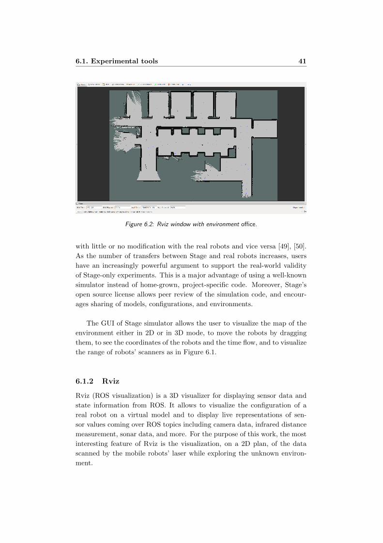
6.1. Experimental tools 41
Figure 6.2: Rviz window with environment office.
with little or no modification with the real robots and vice versa [49], [50].
As the number of transfers between Stage and real robots increases, users
have an increasingly powerful argument to support the real-world validity
of Stage-only experiments. This is a major advantage of using a well-known
simulator instead of home-grown, project-specific code. Moreover, Stage’s
open source license allows peer review of the simulation code, and encour-
ages sharing of models, configurations, and environments.
The GUI of Stage simulator allows the user to visualize the map of the
environment either in 2D or in 3D mode, to move the robots by dragging
them, to see the coordinates of the robots and the time flow, and to visualize
the range of robots’ scanners as in Figure 6.1.
6.1.2 Rviz
Rviz (ROS visualization) is a 3D visualizer for displaying sensor data and
state information from ROS. It allows to visualize the configuration of a
real robot on a virtual model and to display live representations of sen-
sor values coming over ROS topics including camera data, infrared distance
measurement, sonar data, and more. For the purpose of this work, the most
interesting feature of Rviz is the visualization, on a 2D plan, of the data
scanned by the mobile robots’ laser while exploring the unknown environ-
ment.

42 Chapter 6. Experimental results
Figure 6.3: Environments used for experiments.
The partial maps explored by the robots are sent to the BS which merges
them into a unique map of the environment and publishes it on the appropri-
ate ROS topic. Rviz subscribes to this topic and shows the explored map,
as well as the partial maps of the single robots (hidden for clarity in the
figures represented in this chapter). By subscribing to another topic, Rviz
can also show the physical positions of the communication graph vertices
and highlight those that are assigned as goals to the mobile robots.
Figure 6.2 shows a partially explored map of an environment used for
our experiments. The thick black lines correspond to walls and obstacles,
the white area is the explored free space, and the white irregular bound-
aries represent the frontiers to be explored. The blue points spread on the
floor plan indicate the physical position of the vertices of the communication
graph.
6.1.3 Environments
We run our simulations in the same indoor environments used in [32], re-
ported in Figure 6.3. Office represents a floor of an office building, with
long narrow hallways, several doors, and many small separate areas. Clut-
tered represents a floor of a damaged building with a large number of debris
and obstacle of different shapes and positions, with both large and narrow
passages. Openspace is a wide, obstacle-free environment with only one big
internal room and several support columns.
The floor plans of all the three environments have actual size of about
80× 60 meters and are in the form of a 800× 600 pixel PNG file (i.e., with
a resolution of 0.1 meters per pixel that only depends on the file in use).

6.1. Experimental tools 43
6.1.4 Robots
The multirobot system is composed of a fixed number of mobile robots,
which is 6, and a base station. The mobile robots have simulated laser scan
sensors, whose data are given in input to the “nav2d”(graph-based) SLAM
modules (http://wiki.ros.org/nav2d), with a range of 10 meters, a field
of view of 180 degrees and an angular resolution of 0.5 degrees. The BS is
not equipped with any sensors and relies on the robots to get information
about the environment.
The simulated robots represent the real-world TurtleBots, which are low-
cost, personal robot kits with open source software (http://www.turtlebot.
com). These robots consist of a mobile base of size 0.36× 0.36× 0.42 meters
able to move and rotate in any direction, are equipped with a 2D/3D dis-
tance sensor (namely the Microsoft KinectR©), a laptop computer or a SBC
(Single Board Computer), and a WiFi transceiver; see Figure 6.4. Turtle-
Bot is designed to be easy to buy, build, and assemble, using off the shelf
consumer products and parts that can be easily created from standard ma-
terials or 3D printed.
Figure 6.4: TurtleBot equipped with Kinect sensor.
Given the battery capacity of real robots and the relatively short time
needed for the exploration of such environments, the issue of power auton-
omy is not taken into account for these simulations.
An odometry error is added to the odometry value returned by the sim-
ulator, which in turn is given as input to the localization module of each
robot. The purpose is to reproduce in simulation the inaccurate movements
occurring in real world due to any malfunction of the wheels or to irregu-
lar floor. Figure 6.2 also highlights the effect of odometry error on robots’
SLAM module: after traveling from the right side of the map to the left one,
robots’ localization is not as precise as at the beginning and consequently

44 Chapter 6. Experimental results
their scans happen not to be perfectly aligned. On the left side, in fact, it is
possible to notice that some laser shots fall outside the black lines and that
the bounds are no longer well defined.
The robots and the BS are also equipped with a simulated wireless com-
munication system. It is used by the BS to broadcast the replan information
and by mobile robots to exchange scan messages and poll messages. The
system employs the Signal communication model described in Section 2.1.2
to emulate a real scenario.
6.1.5 Log data
During the exploration we keep track of the information logged by the robots
and the BS. All the data are collected at each time step; the timestamps of
such time steps are saved, as well.
• Explored area: the amount of area of the environment explored by
the robot team, in terms of number of pixels of the map known to the
BS. The measure is then converted into squared meters and percentage
over the total area, for a more significant analysis.
• Distance traveled: the sum, over the whole team, of distance trav-
eled by every robot from its own initial position to the current position.
It is measured in meters.
• Disconnection time: the incremental time not in communication
with the BS for every robot. At any time step, if a robot is not
in communication with the BS (either in direct communication or by
means of other teammates which serve as relay), its disconnection time
is incremented by one.
At the end of the exploration, another kind of information is collected,
concerning the graph of the environment and its edges, to compare the
benefits given by our two algorithms in terms of number of edges added:
• Incidence matrix: theN×N symmetric matrix, whereN is the num-
ber of vertices of the communication graph G introduced in Chapter
3, contains 1 in cell i, j if vertices i and j are able to communicate, 0
otherwise.
• Edges added by addition: the number of edges added to the graph
according to the edge addition algorithm.

6.2. Evaluation procedure 45
• Edges added by prediction: the number of edges added to the
graph according to the edge prediction algorithm. Since the GP is pe-
riodically trained with new available samples (and so the model itself
changes), at each replanning computed by the BS the edges added at
the previous iterations are removed from the graph and substituted
with those of the current iteration. We store the number of edges
added at each iteration, then we only consider the average number of
edges added over the whole exploration.
6.2 Evaluation procedure
Given the expected applications for this work in the scope of search and res-
cue, the main objective of our experiments is, of course, to look for the fastest
exploration of the environment where robots are deployed. The fastest ex-
ploration means that our multirobot system has to maximize the explored
area in a given time (or to explore the whole area in the shortest time). This
makes the explored area the most important log data to consider for evalu-
ating the performance of the system. As said before, we do not consider any
constraint on the autonomy of the robots. Data about the distance traveled
by the team of robots is an indirect measure of the performance of the sys-
tem: for the same explored area, a small traveled distance means that the
robots have been moved by the BS in a smarter way on the environment
avoiding retraversing already known parts of the map.
On the other hand, there is a critical constraint to consider for search
and rescue applications: the communication among robots and, more im-
portant, between robots and the BS. The whole system must be set in order
to avoid any possible interruption of communication, both for exchanging
messages about the map and for receiving indications from the BS. More
specifically, since we are in a simulated scenario, the settings must avoid
any “false positive” communication that could let robots exchange simu-
lated messages even if in the same real condition they would not be able to
communicate.
This gives rise to an important trade-off that affects our experiments
between the necessity for a fast exploration of the environment and the
guarantee that robots can connect to the BS when reaching their goals. For
running our experiments, we address this issue by employing two different
settings that concern the edge addition algorithm introduced in Section 4.1,

46 Chapter 6. Experimental results
and in particular the parameters α and β. In fact, by tuning the radius
within which a robot is assigned to a vertex of the graph and the threshold
of signal strength above for which the communication between vertices is
possible, we can obtain different behaviors of the multirobot system during
exploration and, consequently, different results in our experiments.
A hard setting aims at guaranteeing that the communication in the sim-
ulation is the same as in the reality: to be as conservative as possible, we
set α = 3 m and β = −80 dB in order to ensure that an edge is added to
the graph if and only if the two vertices at its ends are able to communicate
according to the signal power model. This setting, which has been tested on
real robots in [10], ensures that an edge added to the graph implies a real
communication between the related vertices.
A soft setting allows to add new edges (i.e., potentially, new reachable
goals for the robots) more “easily” to the map: being less conservative but
still guaranteeing an adequate level of confidence on the possibility of com-
munication between the two vertices connected by the new edge, we set
α = 4 m and β = −85 dB. With this setting, in general, it might be no
always true that an edge added to the graph implies a real communication.
However, since we are working in simulation, we can ensure this property.
This is because the current system does not dispose of any “backup strat-
egy” to be used to regain connection in presence of false positives.
We also pay particular attention to the initial positions of the robots
in the environment: in each map, we place the team of robots where, in a
real scenario, the robots can be physically introduced into the building they
have to explore (e.g., at the entrance or close to the stairwell). Thus, robots
are never placed in the middle of the floor plan, instead they are more likely
to be placed near some wall; of course, in this way robots cannot move in
any direction from the beginning and they are forced to move towards the
centre of the map, and this affects the performance of the multiagent sys-
tem. Moreover, in all the environments, we place by convention the BS in
the same position as the first robot of the team. Figure 6.5, for instance,
shows the initial positions of the robots in environment office.
The objective of these experiments is to show the benefits given by the
implementation of our two algorithms, namely edge addition (Section 4.1)
and edge prediction (Section 4.2). Thus, we want to compare the perfor-
mance of the multirobot system in the following different modes:

6.2. Evaluation procedure 47
Figure 6.5: Initial positions of robots in office.
• Basic: the multirobot system runs “as is”, i.e., as we inherited from
[32] with no additional enhancement or optimization.
• Edge addition: the simple mode is enriched with our edge addition
algorithm.
• Edge prediction: the simple mode is enhanced with the Gaussian
Process.
• Combination: the multirobot system runs with both the edge addi-
tion and the edge prediction algorithms.
For each environment and for each mode, we perform 5 runs with a du-
ration of 20 minutes. This duration does not allow a complete exploration of
the environments in exam, but is long enough to yield relevant and significa-
tive data to analyze offline in the log files. The data about explored area and
distance traveled collected in every group of 5 runs are plotted, separately,
into graphs that indicate, according to the elapsed time, the average value
and the corresponding variance. The data about the number of edges in the

48 Chapter 6. Experimental results
Figure 6.6: Building a communication map over office with an increasing number of
samples in the training set of the GP (from left to right, top to bottom).
graph and the number of edges added by the two algorithms are collected
at the end of each run and stored into tables, in form of average value and
variance.
At last, when running the training of the Gaussian Process in the edge
prediction algorithm, we collect another data useful for visualizing the signal
power strength over the whole environments, at the end of the exploration.
The collection of data works as follows: anytime the GP is trained with
available samples, a process computes – asynchronously with respect to the
exploration task – the predicted value and the corresponding confidence of
the signal power strength between the BS and any point that is a vertex of a
1×1 m custom grid overlaid on the floor plan. Then, a 3D map is computed
to plot, for each point of the map, the value of the signal power strength from
there to the BS. This map highlights the propagation of the signal over the
environments according to its obstacles: for instance, it shows high values
– therefore good signal strength – in correspondence of hallways or empty
rooms and conversely, low values in correspondence of walls, as in Figure 6.6.

6.3. Parameters 49
6.3 Parameters
Before starting any simulated exploration run, the system needs to receive
several inputs to set some parameters in Stage. Some of them concerns the
behavior of the robots during the exploration; others are used to set thresh-
olds required by the communication strategies the system employs.
The parameters related to exploration are:
• Big distance: maximum distance between any two points in the map.
Since all our environments have a rectangular shape, the big distance
is equal to the diagonal of the 80× 60 m floor plan – i.e., 100 m. This
parameter is used to compute the utility of the frontiers that have to
be explored: the closer the frontiers are to the robots, the more likely
they are going to be assigned as goals to the robots.
• Grid resolution: the unit area of the map. A grid resolution of
0.15 means that the floor plan is divided into 0.15 × 0.15 m atomic
parts – i.e., the simulated robots cannot distinguish any detail of the
map smaller than this. A greater grid resolution would increase the
precision in robot localization and obstacle identification through laser
scanning, but a lower grid resolution increases the performance of
the system by requiring less computational effort.
• Stuck threshold: the time limit after which robots that are stuck
into any obstacle, either real or fake, are forced to move in any possible
direction, of course without crashing against a real obstacle. After
some preliminary experiments, this is set to 20 s.
• Replanning threshold: the minimum percentage of robots in ready
state (i.e., that have reached their destinations), over the whole robot
team, that the BS has to wait before replanning. We set this param-
eter to 0.1, meaning that the BS computes a new deployment as soon
as only one robot is ready. This value has been chosen based on the
observations in [32], where the authors state that with this replanning
threshold the system has the best performance.
The parameters related to communication are:
• Communication range: safe range within which the communication
is ensured, according to the conservative Circle model. Given the
features of our environments and the capabilities of WiFi modules, we

50 Chapter 6. Experimental results
can ensure the communication among robots within a radius of 15 m.
Increasing this value would enhance the performance of the system
but would make the simulation less realistic.
• Signal power strength: two robots can communicate based on the
signal strength power between their positions. The communication
strength we adopt is defined in [35] and works as follows:
S = Pd0 − 10×N × log10
dmd0×min(nW,C)×WAF, (6.1)
where we set the signal strength Pd0 = −38 dB at the reference dis-
tance d0 = 1 m, the rate of the path loss N = 2.3, the wall attenu-
ation factor WAF = 3.37, and the maximum number of walls where
the attenuation factor needs to be considered C = 5. The variable
parameters dm and nW represent, respectively, the distance and the
number of obstructing walls between the two robots. The latter de-
pends on the number of pixels per wall (i.e., the thickness of a wall),
which is set to 5, given the floor plans of our environments. We use
this model because it takes into account the degradation derived by
the obstacles and so it models a real setting in a better way. Another
reason to choose this communication model is the possibility to fur-
ther constrain it in special cases, for example, using a shorter distance
Line-of-Sight.
• Noise variance: a white, zero-mean noise is added to the power
strength computed as explained before. The variance of such noise is
1.
• Power cutoff : the signal power threshold below which the commu-
nication is assumed not to be possible is −93 dB.
power strength− noise > power cutoff (6.2)
• Frequency of polling messages: robots acquire polling messages
for measuring the signal power strength among them at regular in-
tervals of time. We set the timer poll messages to 1 s, in order to
collect as many data as possible while robots are moving around in
the environment. A higher value would potentially cause the loss of
data collected when robots move in some unexplored location.
• Frequency of polling messages for GP: not all the poll messages
collected by the robot team are used to train the GP that builds the

6.4. Results 51
communication map of the environment. To keep the training time
bounded, we add to the training set only one poll message out of
thirty taken, i.e., the timer poll messages gp is set to 30 s.
• Threshold power GP: a new edge is added to the communication
graph only if its predicted signal power strength, taken into account
its confidence, is above the threshold γ set to −93 dB.
prediction− 2× predicted standard deviation > γ (6.3)
• Threshold distance GP: in order to avoid adding too many similar
samples to the training set, due to the spatial correlation of the GP, a
new sample is added to the training set H (as shown in Section 4.2)
only if its distance from any other existing samples is greater than 2 m.
With a smaller threshold, more samples would be added to the training
set, but they would carry less meaningful information because of their
strong correlation. Moreover, adding more samples would affect the
time required to train the model, hence the computation time would
increase drastically.
• Timer GP training: the GP is trained asynchronously, with respect
to the exploration task, every 45 s. If one training phase exceeds the
timer gp training due to the high number of samples, the next one
starts as soon as possible right after that. A shorter interval would
require an higher computational effort due to the increased number
of iterations, whereas a longer interval would potentially lead the BS
to plan too many consecutive new deployments based on the same
knowledge of the communication opportunities without any additional
information given by the GP.
6.4 Results
In this section we present the results obtained with our method. For each
environment, we report the explored area and the traveled distance as a
function of time, the percentage of edges added by our two algorithms (with
respect to the total number of edges in the graph at the end of the explo-
ration) and the communication map built by means of the Gaussian Process.
We call “explorable area” the area of the floor plan that is physically reach-
able by the mobile robots, i.e., that is not occupied by walls or obstacles; it
is computed by counting the white pixels of the image over the total number

52 Chapter 6. Experimental results
of pixels.
With regard to communication maps, we recall that they can give an
estimate of the signal power strength about any two pairs of physical loca-
tions. We also remind that, according to the timer poll messages gp, only
1 poll message – collected every 1 s by the robots – out of 30 is added as a
sample in order to limit the size of the training set of the GP generating the
communication map. Lastly, we specify that data plotted under the name
of “communication map” are the 2D-projection of the real 4D-map.
Since we launch 5 runs for each of the 4 modes (basic, edge addition,
edge prediction and combination), data are reported in the form of aver-
age value – over the runs of each mode – and the corresponding standard
deviation. More specifically, the charts about explored area and traveled
distance contain one rectangle per mode, which plots the average value,
with the corresponding error bar, and gaps separate the instants of time in
which data were collected; the tables about added edges contain, for each
mode, the average total number of edges in the graph at the end of the runs,
the average number of edges added by our algorithms and the correspond-
ing percentage of added edges with respect to the total number of edges in
the graph. The total number of edges in the graph is computed by count-
ing the “1”s in the incidence matrix of the graph introduced in Section 6.1.5.
For the following experiments, we use the aforementioned hard setting
to be as conservative as possible on communication capabilities: this allows
on one side the addition of few, safe edges by means of the edge addition
and on the other side a wider addition of edges by exploiting the features of
GPs in the edge prediction.
A further series of experiments, performed in soft setting, is presented
in Section 6.4.4 for the sake of completeness.
6.4.1 Office
The environment office presents long narrow hallways, several doors, and
many small separate areas. The robot team is initially positioned in the up-
per right corner, close to the stairwell from which they might be realistically
introduced into the building, divided in two columns of three robots each
facing back-to-back as in Figure 6.5.

6.4. Results 53
Figure 6.7: Explored area and traveled distance in office.
Explored area (m2) Traveled distance (m)
avg std dev avg std dev
Basic 282.95 12.61 405.20 52.30
Edge addition 312.16 32.95 419.00 51.61
Edge prediction 298.65 45.11 334.00 38.57
Combination 326.69 19.15 338.20 38.98
Table 6.1: Exploration results for office at t = 20 min.
The explored area and the traveled distance are shown in Figure 6.7
and Table 6.1. One can notice that the edge addition algorithm does not
bring any significant benefit with respect to the basic mode, whereas the
edge prediction starts enhancing the exploration after 10 minutes and keeps
growing until the end; the combination of the two algorithms, as easily con-
ceivable, gives the best improvement to the exploration with respect to the
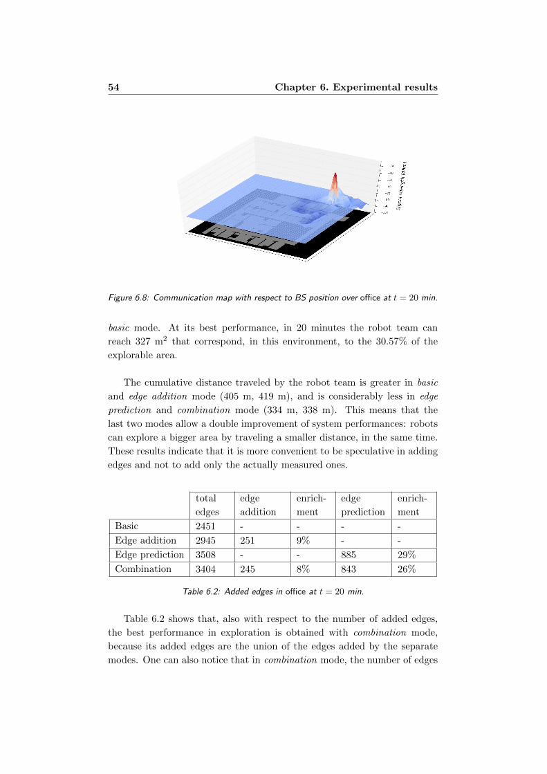
54 Chapter 6. Experimental results
Figure 6.8: Communication map with respect to BS position over office at t = 20 min.
basic mode. At its best performance, in 20 minutes the robot team can
reach 327 m2 that correspond, in this environment, to the 30.57% of the
explorable area.
The cumulative distance traveled by the robot team is greater in basic
and edge addition mode (405 m, 419 m), and is considerably less in edge
prediction and combination mode (334 m, 338 m). This means that the
last two modes allow a double improvement of system performances: robots
can explore a bigger area by traveling a smaller distance, in the same time.
These results indicate that it is more convenient to be speculative in adding
edges and not to add only the actually measured ones.
total
edges
edge
addition
enrich-
ment
edge
prediction
enrich-
ment
Basic 2451 - - - -
Edge addition 2945 251 9% - -
Edge prediction 3508 - - 885 29%
Combination 3404 245 8% 843 26%
Table 6.2: Added edges in office at t = 20 min.
Table 6.2 shows that, also with respect to the number of added edges,
the best performance in exploration is obtained with combination mode,
because its added edges are the union of the edges added by the separate
modes. One can also notice that in combination mode, the number of edges
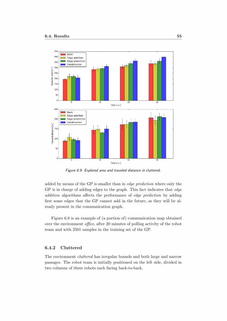
6.4. Results 55
Figure 6.9: Explored area and traveled distance in cluttered.
added by means of the GP is smaller than in edge prediction where only the
GP is in charge of adding edges to the graph. This fact indicates that edge
addition algorithms affects the performance of edge prediction by adding
first some edges that the GP cannot add in the future, as they will be al-
ready present in the communication graph.
Figure 6.8 is an example of (a portion of) communication map obtained
over the environment office, after 20 minutes of polling activity of the robot
team and with 2501 samples in the training set of the GP.
6.4.2 Cluttered
The environment cluttered has irregular bounds and both large and narrow
passages. The robot team is initially positioned on the left side, divided in
two columns of three robots each facing back-to-back.

56 Chapter 6. Experimental results
Figure 6.10: Communication map with respect to BS position over cluttered at t = 20
min.
Explored area (m2) Traveled distance (m)
avg std dev avg std dev
Basic 339.15 26.35 207.30 26.59
Edge addition 338.94 20.74 200.44 9.66
Edge prediction 362.55 16.92 212.26 12.23
Combination 399.13 9.69 213.57 12.57
Table 6.3: Exploration results for cluttered at t = 20 min.
The explored area and the traveled distance are shown in Figure 6.9 and
Table 6.3. The system performance in the basic mode is almost equal to
those in edge addition and edge prediction, whereas the combination mode
reaches considerably better results, in particular from 10 minutes on. At
its best performance, in 20 minutes the robot team can reach 399 m2 that
correspond, in this environment, to the 30.65% of the explorable area.
The cumulative distance traveled by the robot team does not vary signif-
icantly in all the modes: in fact, the rectangles have almost the same height
in the whole chart and end up at about 210 m. This result is instead very
different from the one obtained in office because of the more homogeneous
distribution of empty spaces and obstacles over the floor plan.
Table 6.4 shows that, also with respect to the number of added edges,
the best performance is in combination mode. As in the previous environ-
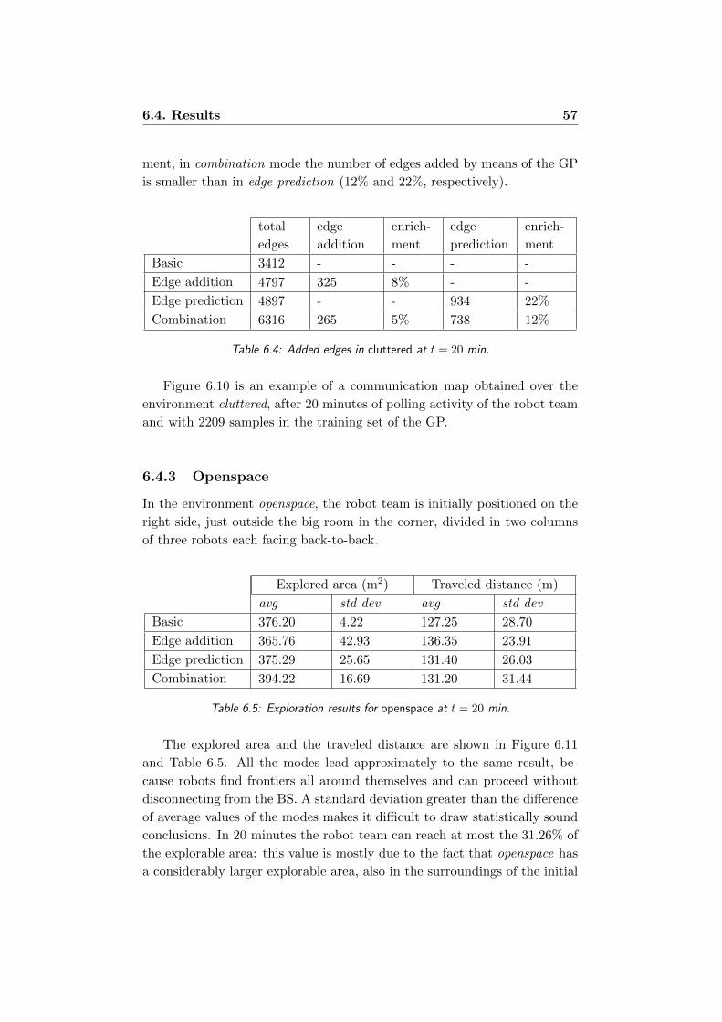
6.4. Results 57
ment, in combination mode the number of edges added by means of the GP
is smaller than in edge prediction (12% and 22%, respectively).
total
edges
edge
addition
enrich-
ment
edge
prediction
enrich-
ment
Basic 3412 - - - -
Edge addition 4797 325 8% - -
Edge prediction 4897 - - 934 22%
Combination 6316 265 5% 738 12%
Table 6.4: Added edges in cluttered at t = 20 min.
Figure 6.10 is an example of a communication map obtained over the
environment cluttered, after 20 minutes of polling activity of the robot team
and with 2209 samples in the training set of the GP.
6.4.3 Openspace
In the environment openspace, the robot team is initially positioned on the
right side, just outside the big room in the corner, divided in two columns
of three robots each facing back-to-back.
Explored area (m2) Traveled distance (m)
avg std dev avg std dev
Basic 376.20 4.22 127.25 28.70
Edge addition 365.76 42.93 136.35 23.91
Edge prediction 375.29 25.65 131.40 26.03
Combination 394.22 16.69 131.20 31.44
Table 6.5: Exploration results for openspace at t = 20 min.
The explored area and the traveled distance are shown in Figure 6.11
and Table 6.5. All the modes lead approximately to the same result, be-
cause robots find frontiers all around themselves and can proceed without
disconnecting from the BS. A standard deviation greater than the difference
of average values of the modes makes it difficult to draw statistically sound
conclusions. In 20 minutes the robot team can reach at most the 31.26% of
the explorable area: this value is mostly due to the fact that openspace has
a considerably larger explorable area, also in the surroundings of the initial

58 Chapter 6. Experimental results
Figure 6.11: Explored area and traveled distance in openspace.
position of the robots that are free to move and explore in any direction
from the beginning.
Also for the traveled distance, the very high standard deviation does not
allow a sound analysis of the performance. In this environment, the perfor-
mance of the exploration are worse than in the others because of the limited
range of the laser scanner mounted on robots cannot catch enough valid
landmarks in such a wide, empty space. Basically, robots move blindly “in
the middle of nowhere”, i.e., they cannot see any point of reference around
them and cannot smartly decide where to go. The small squares spread over
the floor plan, which represent support columns, act as landmarks for the
robots to help them orient themselves within the map.
As it might be expected, none of the methods seems to be able to pro-
vide significant advantages with respect to the basic strategy, both in terms
of mapped area and average traveled distance. Such a difference in perfor-

6.4. Results 59
Figure 6.12: Communication map with respect to BS position over openspace at t = 20
min.
mance gains compared to office is probably due to the following fact. Being
the openspace environment simpler, in the sense that a robot can almost
always reach a given position by moving straightly, it rarely happens that
robots have to travel long distances to construct relay chains connecting
new frontiers to the BS. Therefore, even when the chain is composed by 2-3
robots due to the lack of a direct frontier-BS communication link (which
could have been learned with one of the other methods), the latter is still
able to receive map updates at a fast pace. This does not happen in the
office environment, where relay chains far from the current ones might re-
quire long times to be formed.
total
edges
edge
addition
enrich-
ment
edge
prediction
enrich-
ment
Basic 8666 - - - -
Edge addition 8562 488 6% - -
Edge prediction 14031 - - 1213 10%
Combination 10102 501 5% 971 10%
Table 6.6: Added edges in openspace at t = 20 min.
With regard to the number of added edges, Table 6.6 shows that it is
relatively small in any mode, with respect to the other environments. This
happens because the largest part of the edges is added to the graph only by
checking the constraint on the communication range: in fact, the graph in

60 Chapter 6. Experimental results
Figure 6.13: Comparison of explored area and traveled distance in office under different
settings.
openspace contains many more edges than the graphs of the other environ-
ments (an average of 10340 against 3077 in office and 4856 in cluttered).
Figure 6.12 is an example of communication map obtained over the en-
vironment openspace, after 20 minutes of polling activity of the robot team
and with 2310 samples in the training set of the GP.
6.4.4 Complementary experiments
We report additional experiments conducted in environment office with soft
setting to justify our choice of using hard setting for the previous experi-
ments. The different setting only affects the edge addition and combination
modes; hence, the following charts and tables only report those data series
for clarity.

6.4. Results 61
Explored area (m2) Traveled distance (m)
avg std dev avg std dev
Edge addition (soft) 284.51 11.80 409.40 31.93
Edge addition (hard) 312.61 32.95 419.00 51.61
Combination (soft) 294.96 31.65 336.60 45.04
Combination (hard) 326.69 19.15 338.20 38.98
Table 6.7: Exploration results in office at t = 20 min under different settings.
The explored area and the distance traveled are shown in Figure 6.13 and
Table 6.7. The system performance in combination mode under hard setting,
which reaches 327 m2, outperforms from the three other cases; among those,
anyway, the edge addition under hard setting is the best. In 20 minutes the
robot team can reach on average the 29.91% of the explorable area under
hard setting, against the 27.11% under soft setting.
Regarding the traveled distance, it is clearly visible a bifurcation in the
plotted data, even though it regards the mode instead of the setting: com-
bination mode under both settings is more efficient than edge addition (re-
spectively, an average of 337 m against an average of 414 m of cumulative
traveled distance). This gives strong support to the benefit given by combi-
nation.
total
edges
edge
addition
enrich-
ment
edge
prediction
enrich-
ment
Edge addition (soft) 2936 625 21% - -
Edge addition (hard) 2945 251 9% - -
Combination (soft) 3857 506 14% 638 17%
Combination (hard) 3404 245 8% 843 28%
Table 6.8: Added edges in office at t = 20 min under different settings.
Table 6.8 shows that, also with respect to the number of added edges,
the best performance is under hard setting. On the other hand, one can
also notice that in edge addition mode, the soft setting offers clearly the
best performance. In fact, when the GP is not active, the edges can only
be added to the graph by means of our first algorithm and consequently, as
said in Section 6.2, the less restrictive soft setting allows the BS to add more
edges. When the GP is active in combination mode, instead, it contributes

62 Chapter 6. Experimental results
to add edges thus reducing the activity of edge addition algorithm and the
effect of less restrictive settings.
As far as edge prediction is concerned, we cannot make a comparison
– and highlight differences – between hard setting and soft setting because
parameter relaxation only affects edge addition.

Chapter 7
Conclusions and future work
This work enhanced the communication model and the functionalities of an
existing multirobot system that explores unknown environments.
The thesis started from a multirobot system dedicated to the explo-
ration of an initially unknown environment in which robots could exchange
knowledge under the conservative assumption that the BS could send its
directives to robots within a given range of communication. Such a system
showed performance in the exploration task that was somehow limited.
To achieve our objective, we brought the following changes to the system:
1. We overcame the conservative communication model based on range
(Circle model) defining the possibility to communicate according to
the signal power strength (Signal model).
2. We added a filter node in ROS that allows the robots to exchange
information about the environment only with those in communication,
even through a multihop chain. This node is used only in simulation
to mimic real communications.
3. We built a polling mechanism for collecting information about the
signal power strength between any pair of robots moving around in
the environment.
4. We implemented an algorithm for adding edges to the communication
graph by using the measures of signal power strength made by robots
nearby unlinked vertices of the graph.

64 Chapter 7. Conclusions and future work
5. We implemented a second algorithm for adding edges exploiting the
prediction on signal power strength between two unconnected vertices
of the communication graph given by a Gaussian Process.
6. We combined the two algorithms to add as many edges as possible,
based both on real measurements and on predictions, in order to let
the robots use the best possible information to move farther and ex-
plore a bigger area.
We validated our work with experiments conducted in Stage simulator on
three indoor environments with different features (long hallways with many
small rooms; spread irregular obstacles and narrow passages; large empty
space) and with two different settings that regulate the conservativeness
of the behavior of our algorithms. The experiments support the following
conclusions:
• After the implementation of our algorithms, both individually and
in combination, the multirobot system was able to explore a larger
area while traveling a shorter distance when compared to the original
system based on a Circle communication graph.
• The addition of edges according to measures brought, especially in
combinations with the addition of edges by means of predictions, big-
ger benefits with restrictive parameters than with relaxed parameters.
Indeed, it is better to have less, but reliable, edges than more, but less
reliable, edges.
• Predictions allow to add more edges to the communication graph com-
pared to actual measurements, so they are in general the main respon-
sible of the improved performance of the system.
• Not all the environments benefit in the same measure from our work: a
regularly fragmented space obtains better results due to the enhanced
communication model. Specifically, we can state that in environments
such as office, the coordination is more relevant than in others, there-
fore providing a good communication model leads to better results.
Future works in the context of our thesis may follow two main direc-
tions: i) generalize the problem so as to remove completely or partially our
initial assumptions and ii) develop other algorithms or improve the existing
ones in order to obtain a further enhancement of exploration abilities of the

65
multirobot system.
The former aims at building a multirobot system that is more realistic
in its components and more adaptable to the features of real environments.
Some examples are the following:
• Extension of the team composition: this thesis has extensively
analyzed a system with a fixed number of homogeneous robots. Fu-
ture work can explore different initial team configurations as well as
heterogeneity among the team to split the exploration effort based on
the capabilities of different agents.
• Extension of the exploration strategy: in this work we analyzed
a specific strategy that maximizes the explored area, for evaluating
the system performance in the exploration task. A possible extension
is to consider, instead, a strategy that minimizes the distance traveled
by the robots in order to increase their operating time.
• Dynamic environment: a strong assumption is that the environ-
ment cannot change during the exploration task. In real cases, espe-
cially in search and rescue applications, a floor plan might change due
to the breakdown of a wall that reveals new spaces, the collapse of the
ceiling that releases debris, the appearance of moving obstacles. An
enhanced multirobot system should be able to cope with these possi-
bilities.
The latter direction for future work plans to add new functionalities to
our system or to improve the existing ones. Here are some examples:
• Multi-team exploration: instead of performing both the explo-
ration of the environment and the construction of a communication
map with an unique team of equivalent robots, the two tasks could
be separated by splitting the robot team. Robots of one sub-team
move randomly in the environment while measuring the signal power
strength and building a communication map. Robots of the other team
move according to the communication map to explore new frontiers.
• Favoring the communication task: the robot team in this work
focused its activity on exploring the environment, considering the issue
of communication only as a by-product of exploration. Alternatively,
it is possible to favor the communication task by moving the robots

66 Chapter 7. Conclusions and future work
around in the environment to the best locations to collect informa-
tion about the signal power strength in order to build more accurate
communication maps.
• Enhance the edge addition algorithm: in this work we fixed at the
beginning of the exploration the value for the communication range α
and the power cutoff β. An improvement could be to correlate those
two parameters to each other. Specifically, the closer a robot is to a
matching vertex, the less restrictive the power threshold should be and
vice versa.
• Enhance the edge prediction algorithm: in this work we fixed a
value for the frequency of polling messages for GP, collecting data on
the signal power strength among robots every fixed interval of time so
as to limit the growth of the training set and the consequent computa-
tional effort required. A further development could consist in making
this parameter variable, and more precisely increasing over time, in
order to train the GP more frequently at the beginning when only
few samples are available and less frequently later on when samples
increase in number.

Bibliography
[1] A. Farinelli, L. Iocchi, and D. Nardi. Multirobot systems: A classifica-
tion focused on coordination. In Proceedings of IEEE Transactions on
Systems, Man and Cybernetics, volume 34, pages 2015–2028, 2004.
[2] J. Banfi, A. Quattrini Li, N. Basilico, I. Rekleitis, and F. Amigoni.
Strategies for Coordinated Multirobot Exploration with Recurrent Con-
nectivity Constraints. Autonomous Robots, pages 1–20, 2017. To ap-
pear.
[3] F. Amigoni, J. Banfi, and N. Basilico. Multirobot exploration of
communication-restricted environments: a survey. IEEE Intelligent
Systems Magazine, pages 1–12, 2017. To appear.
[4] A. Quattrini Li, R. Cipolleschi, M. Giusto, and F. Amigoni. A
semantically-informed multirobot system for exploration of relevant ar-
eas in search and rescue settings. Autonomous Robots, 40(4):581–597,
2016.
[5] B. Yamauchi. Frontier-based exploration using multiple robots. In
Proceedings of 2nd International Conference on Autonomous Agents,
pages 47–53, 1998.
[6] M. Pei, M. Mutka, and N. Xi. Connectivity and bandwidth-aware real-
time exploration in mobile robot networks. Wireless Communications
Mobile Computing, 13:847–863, 2013.
[7] G.A. Hollinger and S. Singh. Multirobot coordination with periodic
connectivity: Theory and experiments. IEEE Transactions on Robotics,
28(4):967–973, 2012.
[8] N. Stump, V. Michal, and V. Isler. Visibility-based deployment of robot
formations for communication maintenance. In Proceedings of IEEE In-
ternational Conference on Robotics and Automation, pages 4498–4505,
2011.
67

68 BIBLIOGRAPHY
[9] B. Ferris, D. Fox, and N. Lawrence. WiFi-SLAM using Gaussian Pro-
cess latent variable models. In Proceedings of the 20th international
joint conference on Artifical intelligence, volume 7, pages 2480–2485,
2007.
[10] J. Banfi, A. Quattrini Li, N. Basilico, I. Rekleitis, and F. Amigoni.
Multirobot online construction of communication maps. In Proceedings
of IEEE International Conference on Robotics and Automation, pages
2577–2583, 2017.
[11] C.E. Rasmussen and C.K. Williams. Gaussian Processes for Machine
Learning (Adaptive Computation and Machine Learning). The MIT
Press, 2005.
[12] R. Marchant and F. Ramos. Radar: An in-building RF-based user
location and tracking system. In Proceedings of IEEE International
Conference on Robotics and Automation, pages 6136–6143, 2014.
[13] A. Viseras, T. Wiedemann, C. Manss, L Magel, J. Mueller, D. Shutin,
and L. Merino. Decentralized multiagent exploration with online-
learning of gaussian processes. In Proceedings of IEEE International
Conference on Robotics and Automation, pages 775–784, 2016.
[14] A. Singh, F. Ramos, H. D. Whyte, and J. Kaiser. Modeling and decision
making in spatio-temporal processes for environmental surveillance. In
Proceedings of International Conference on Robotics and Automation,
pages 5490–5497, 2010.
[15] F. Amigoni, N. Basilico, and A. Quattrini Li. Moving From ‘How To Go
There?’ to ‘Where To Go?’: Towards Increased Autonomy of Mobile
Robots. In New Trends in Medical and Service Robots, Mechanisms
and Machine Science, pages 345–356. Springer, 2014.
[16] J. Banfi, A. Quattrini Li, N. Basilico, and F. Amigoni. Communication-
constrained multirobot exploration: Short taxonomy and comparative
results. In Proceedings of the IROS workshop on On-Line Decision-
Making in MultiRobot Coordination, 2015.
[17] W. Burgard, M. Moors, C. Stachniss, and F. E. Schneider. Coordinated
multirobot exploration. IEEE Transactions on Robotics, 21(3):376–386,
2005.
[18] H.G. Nguyen, N. Pezeshkian, A. Gupta, and N. Farrington. Maintaining
communication link for a robot operating in a hazardous environment.

BIBLIOGRAPHY 69
In Proceedings of ANS 10th International Conference on Robotics and
Remote Systems for Hazardous Environments, volume 10, pages 256–
263, 2004.
[19] R.C. Arkin and J. Diaz. Line-of-sight constrained exploration for re-
active multiagent robotic teams. In Proceedings of 7th International
Workshop on Advanced Motion Control, pages 455–461, 2002.
[20] A. Pronobis, P. Jensfelt, K. Sjoo, H. Zender, G.M. Kruijff, O.M. Mozos,
and W. Burgard. Semantic modelling of space. In Cognitive Systems,
volume 8 of Cognitive Systems Monographs, pages 165–221. 2010.
[21] D. Fox, J. Ko, K. Konolige, B. Limketkai, D. Schulz, and B. Stewart.
Distributed multirobot exploration and mapping. In Proceedings of the
2nd Canadian Conference on Computer and Robot Vision, pages 1325–
1339, 2005.
[22] A. Franchi, L. Freda, G. Oriolo, and M. Vendittelli. The sensor-based
random graph method for cooperative robot exploration. IEEE/ASME
Transactions on Mechatronics, 14:163–175, 2009.
[23] A. Visser and B.A. Slamet. Including communication success in the es-
timation of information gain for multirobot exploration. In Proceedings
of 6th International Symposium on Modeling and Optimization in Mo-
bile, Ad Hoc, and Wireless Networks and Workshops, pages 680–687,
2008.
[24] V. Spirin and S. Cameron. Rendezvous through obstacles in multiagent
exploration. In Proceedings of International Symposium on Safety, Se-
curity and Rescue Robotics, pages 1–6, 2014.
[25] P. Brass, F. Cabrera-Mora, and J. Gasparri, A. Xiao. Multirobot tree
and graph exploration. IEEE Transactions on Robotics, 27:707–717,
2011.
[26] E. Jensen, L. Lowmanstone, and M. Gini. Communication-restricted
exploration for search teams. In Proceedings of the 13th International
Symposium on Distributed Autonomous Robotic Systems, 2016. To ap-
pear.
[27] M.N. Rooker and A. Birk. multirobot exploration under the constraints
of wireless networking. Control Engineering Practice, 15(4):435–445,
2007.

70 BIBLIOGRAPHY
[28] V. Spirin, S. Cameron, and J.D. Hoog. Time preference for information
in multiagent exploration with limited communication. In Proceedings
of the 14th Towards Autonomous Robotic Systems Conference, pages
34–45, 2013.
[29] W. Sheng, Q. Yang, J. Tan, and N. Xi. Distributed multirobot co-
ordination in area exploration. Robotics and Autonomous Systems,
54(12):945–955, 2006.
[30] A. Howard and G. Sukhatme. An incremental self-deployment algo-
rithm for mobile sensor networks. Autonomous Robots, 13:113–126,
2002.
[31] X. Cheng, D. Du, L. Wang, and B. Xu. Relay sensor placement in
wireless sensor networks. Wireless Networks, 14:346–355, 2008.
[32] J. Banfi, A. Quattrini Li, N. Basilico, I. Rekleitis, and F Amigoni.
Asynchronous multirobot exploration under recurrent connectivity con-
straints. In Proceedings of IEEE International Conference on Robotics
and Automation, pages 5491–5498, 2016.
[33] N. Basilico and F. Amigoni. Exploration strategies based on multi-
criteria decision making for searching environments in rescue opera-
tions. Autonomous Robots, 31:401–417, 2011.
[34] E. A. Jensen, E. Nunes, and M. Gini. Communication-restricted explo-
ration for robot teams. In AAAI Multiagent Interaction without Prior
Coordination Workshop, 2014.
[35] V. Bahl and V. Padmanabhan. Radar: An in-building rf-based user lo-
cation and tracking system. In Proceedings of 19th Annual Joint Con-
ference of the IEEE Computer and Communications Societies, pages
775–784, 2000.
[36] J. Fink and V. Kumar. Online methods for radio signal mapping with
mobile robots. In Proceedings of IEEE International Conference on
Robotics and Automation, pages 1940–1945, 2010.
[37] B. Ferris, D. Hahnel, and D. Fox. Gaussian processes for signal strength-
based location estimation. In Proceeding of 2nd International Confer-
ence on Robotics Science and Systems, volume 2, pages 303–310, 2006.
[38] C. Guestrin, A. Krause, and A. Singh. Near-optimal sensor placements
using Gaussian processes. In Proceedings of the International Confer-
ence on Machine Learning, pages 235–284, 2005.

BIBLIOGRAPHY 71
[39] N. Lawrence. Gaussian process latent variable models for visualiza-
tion of high dimensional data. In Proceedings of Advances in Neural
Information Processing Systems, pages 1783–1816, 2003.
[40] K. Liu, A. Hertzmann, and Z. Popovic. Learning physics-based motion
style with nonlinear inverse optimization. In ACM Transactions on
Graphics (Proceedings of SIGGRAPH), pages 1071–1081, 2005.
[41] C. Stachniss, O.M. Mozos, and W. Burgard. Speeding-up multirobot
exploration by considering semantic place information. In Proceedings
of IEEE International Conference on Robotics and Automation, pages
1692–1697, 2006.
[42] A. Brooks, A. Makarenko, and B. Upcroft. Gaussian process models for
sensor-centric robot localisation. In Proceedings of IEEE International
Conference on Robotics and Automation, pages 56–61, 2006.
[43] A. Pronobis and P. Jensfelt. Large-scale semantic mapping and rea-
soning with heterogeneous modalities. In Proceedings of IEEE Interna-
tional Conference on Robotics and Automation, pages 3515–3522, 2012.
[44] M. Pfingsthorn, B. Slamet, and A. Visser. A scalable hybrid multirobot
SLAM method for highly detailed maps. In Lecture Notes in Computer
Science (including subseries Lecture Notes in Artificial Intelligence and
Lecture Notes in Bioinformatics), volume 5001 LNAI, pages 457–464,
2008.
[45] R. Vincent, D. Fox, J. Ko, K. Konolige, B. Limketkai, B. Morisset,
C. Ortiz, D. Schulz, and B. Stewart. Distributed multirobot explo-
ration, mapping, and task allocation. Annals of Mathematics and Ar-
tificial Intelligence, 52(2-4):229–255, 2008.
[46] M. Quigley, K. Conley, B.P. Gerkey, J. Faust, T. Foote, J. Leibs,
R. Wheeler, and A.Y. Ng. ROS: an open-source Robot Operating Sys-
tem. In ICRA Workshop on Open Source Software, 2009.
[47] R. Vaughan. Massively multiple robot simulations in stage. Swarm
Intelligence, 2:189–208, 2008.
[48] B.P. Gerkey, R.T. Vaughan, and A. Howard. The Player/Stage project:
Tools for multirobot and distributed sensor systems. In Proceedings
of the International Conference on Advanced Robotics, pages 317–323,
2003.

72 BIBLIOGRAPHY
[49] J. Boyoon and S. S. Gaurav. Tracking targets using multiple robots:
The effect of environment occlusion. Autonomous Robots, 13:191–205,
2002.
[50] A. Makarenko, S. Williams, F. Bourgault, and H. F. Durrant-Whyte.
An experiment in integrated exploration. In Proceedings of Intelligent
Robots and Systems, pages 534–539, 2002.

Appendix A
Rviz sequence
Reconstruction of the map of the environment office in Rviz. The sequence
of snapshots shows, at intervals of 5 minutes, the map known to the base
station that merges the scans received by the 6 exploring robots. The thick
black lines correspond to walls and obstacles, the white area is the explored
free space, and the white irregular boundaries represent the frontiers to be
explored.
Figure A.1: Rviz snapshot at time t = 5 min.
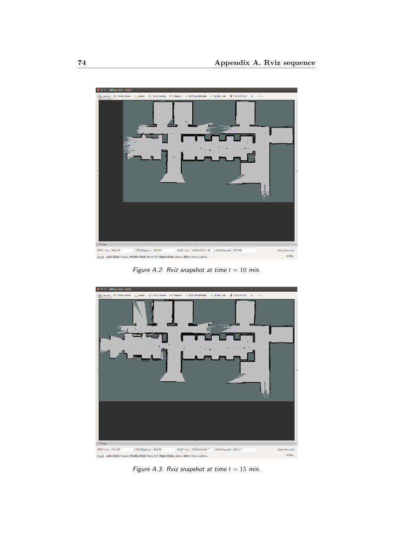
74 Appendix A. Rviz sequence
Figure A.2: Rviz snapshot at time t = 10 min.
Figure A.3: Rviz snapshot at time t = 15 min.

75
Figure A.4: Rviz snapshot at time t = 20 min.
Figure A.5: Rviz snapshot at time t = 25 min.
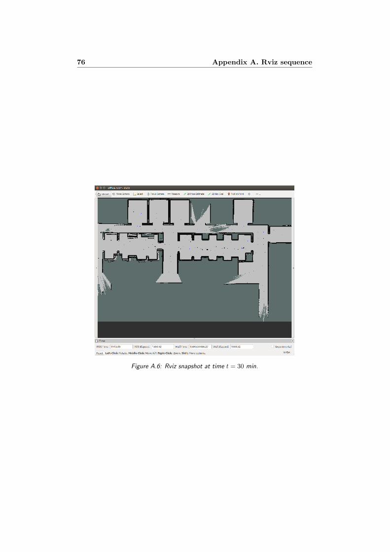
76 Appendix A. Rviz sequence
Figure A.6: Rviz snapshot at time t = 30 min.

Appendix B
Communication map
sequence
Construction of the communication map over the environment office. The
sequence of snapshots shows, at intervals of 5 minutes, for every point of a
1 × 1 m grid overlaid on the floor plan, the predicted values of the signal
strength between such points and the base station. Predictions are based on
measurements collected by the exploring robots that are used as samples in
the training set of a Gaussian Process. The red peak indicates the location
of the base station, high values – therefore good signal strength – correspond
to hallways or empty rooms and low values correspond to walls.
Figure B.1: Communication map with 6 samples as training set.

78 Appendix B. Communication map sequence
Figure B.2: Communication map with 657 samples as training set.
Figure B.3: Communication map with 1410 samples as training set.

79
Figure B.4: Communication map with 1944 samples as training set.
Figure B.5: Communication map with 2232 samples as training set.

80 Appendix B. Communication map sequence
Figure B.6: Communication map with 3088 samples as training set.