Anno Accademico 2020-2021

Politecnico di Torino

DIPARTIMENTO DI AUTOMATICA E INFORMATICA Corso di laurea magistrale in Ingegneria Meccatronica

Elaborato di Tesi

Design of an assistive robot

Candidato: Relatore: Fabio Petracchi Marcello Chiaberge

Correlatore: Luca Carbonari

P a g . | 1

Summary

Introduction ........................................................................................................................................... 2

1 State of the art .................................................................................................................................... 3

1.1 Classification ...................................................................................................................................... 3

1.2 Omnidirectional and pseudo-Omnidirectional robots .................................................................... 10

1.3 Market ............................................................................................................................................. 11

2 Task analysis ..................................................................................................................................... 14

2.1 Person follow task ................................................................................................................................. 15

2.2 Service task ............................................................................................................................................ 17

2.3 Modularity ............................................................................................................................................. 19

3 Kinematic analysis ............................................................................................................................. 21

3.1 Pose Kinematic ...................................................................................................................................... 22

3.1.1 Wheel-ground contact model ................................................................................................. 25

3.2 Velocity kinematic ................................................................................................................................. 27

3.3 Constraint equations ............................................................................................................................. 30

3.4 Direct Kinematics ................................................................................................................................... 31

3.5 Inverse kinematics ................................................................................................................................. 33

3.6 Centre of instantaneous rotation .......................................................................................................... 35

3.7 Operative configurations ....................................................................................................................... 36

4 Trajectory planning ........................................................................................................................... 39

4.1 Parametric definition of the geometric trajectory ................................................................................ 39

4.2 Definition of the motion law ................................................................................................................. 43

5 Mechatronic design ........................................................................................................................... 45

5.1 Generic layout ....................................................................................................................................... 45

5.2 Wheel motor connections ..................................................................................................................... 48

5.3 SPI Bus ................................................................................................................................................... 51

5.4 Proximity Sensors connections .............................................................................................................. 54

5.5 Serial interface ....................................................................................................................................... 56

Conclusion and Further Development ................................................................................................... 59

References ........................................................................................................................................... 61

Ringraziamenti ..................................................................................................................................... 62

P a g . | 2

Introduction

As reported by the UN (1) the expected growth of the population older than 60 years is from

18.8% in 2000 to 34.2% in 2050, showing an exponential growth of the elder people in the world.

Hence an always bigger number of people will show a substantial decrease of their mobility and

capability in doing daily tasks.

Moreover, an affordable aid with the daily house task will result of interest for everyone, not only

the elderly.

As a matter of fact, a solution to this issue can be provided by the recent development of

automation.

This Thesis offer as an answer an innovative platform for wheeled mobile robots (WMR) designed

for assistive purposes.

Giving assistance inside a house concern a lot of mobility issues, because the WMR must be able

not only to navigate into an indoor environment without causing any trouble but also to react

rapidly to unknown modifications at the environment.

To deal with these problems it is necessary a sophisticated software capable of an accurate path

planning, but it isn’t sufficient.

To follow complex trajectory or react rapidly to an uncommon obstacle on the path the platform

structure must be advanced enough; for example the most used actuation for assistive WMR is the

simple Differential Drive, as we will see in the chapter 1, but this typology of platform has a very

restricted mobility making useless a sophisticate path planning.

In this scenario, finding a modular solution could be very interesting for the market, because not

only allows to design the software separately but also can be implemented for very different

applications, opening many more opportunity.

In addition, it’s fundamental that this platform will be as cheaper as possible in order to put this

platform into production.

P a g . | 3

Chapter 1

State of the art

In this chapter will be analysed the state of the art of the Wheeled Mobile Robot (WMR).

In the section 1.1 a classification of the various kind of WMR is done. Primarily a wheel

classification is carried out, then three design variables are defined: degree of manoeuvrability

(δ𝑀), degree of mobility (δ𝑚) and degree of steerability (δ𝑠). Finally manipulating these three

design variables, five different structures determined.

In the section 1.2 the differences between omni-directional and pseudo-omnidirectional WMR is

analysed in order to determine pros and cons of these two structures.

Inside the section 1.3 there is a view of what actually the market offers in terms of WMR designed

specifically for assistive purpose.

1.1 Classification

First, a WMR classification with respect to kinematic and dynamic properties is essential. Such

analysis can be found in (2), where three design variables are defined: degree of manoeuvrability

(δ𝑀), degree of mobility (δ𝑚) and degree of steerability (δ𝑠).

Such variables depend only on the type and number of wheels (and if they are on the same axis)

and not on other structural properties of the platform.

There are essentially two kind of wheels: Conventional Wheel and Omni-wheels.

For a Conventional wheel the contact between wheel and ground is supposed to satisfy pure

rolling condition without slip. They can be Fixed, Centered orientable or Off-centered (Castor).

P a g . | 4

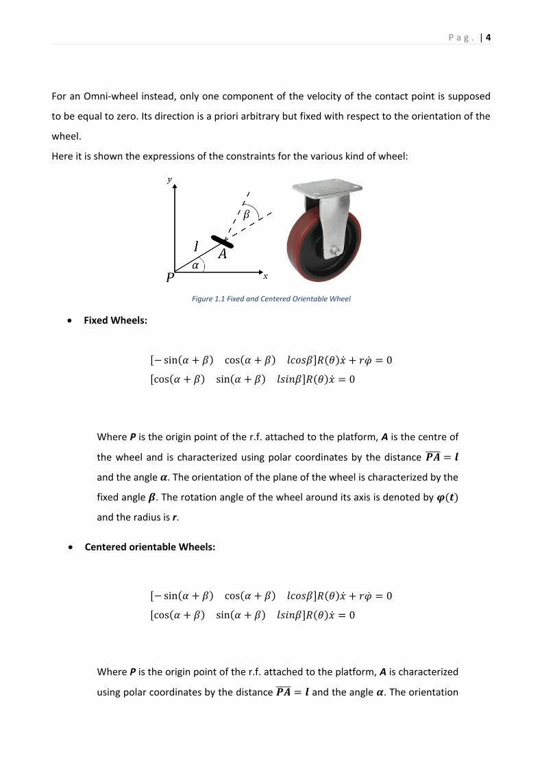
For an Omni-wheel instead, only one component of the velocity of the contact point is supposed

to be equal to zero. Its direction is a priori arbitrary but fixed with respect to the orientation of the

wheel.

Here it is shown the expressions of the constraints for the various kind of wheel:

Figure 1.1 Fixed and Centered Orientable Wheel

• Fixed Wheels:

[− sin(𝛼 + 𝛽) cos(𝛼 + 𝛽) 𝑙𝑐𝑜𝑠𝛽]𝑅(𝜃)�̇� + 𝑟�̇� = 0

[cos(𝛼 + 𝛽) sin(𝛼 + 𝛽) 𝑙𝑠𝑖𝑛𝛽]𝑅(𝜃)�̇� = 0

Where P is the origin point of the r.f. attached to the platform, A is the centre of

the wheel and is characterized using polar coordinates by the distance 𝑷𝑨̅̅ ̅̅ = 𝒍

and the angle 𝜶. The orientation of the plane of the wheel is characterized by the

fixed angle 𝜷. The rotation angle of the wheel around its axis is denoted by 𝝋(𝒕)

and the radius is r.

• Centered orientable Wheels:

[− sin(𝛼 + 𝛽) cos(𝛼 + 𝛽) 𝑙𝑐𝑜𝑠𝛽]𝑅(𝜃)�̇� + 𝑟�̇� = 0

[cos(𝛼 + 𝛽) sin(𝛼 + 𝛽) 𝑙𝑠𝑖𝑛𝛽]𝑅(𝜃)�̇� = 0

Where P is the origin point of the r.f. attached to the platform, A is characterized

using polar coordinates by the distance 𝑷𝑨̅̅ ̅̅ = 𝒍 and the angle 𝜶. The orientation

P a g . | 5

of the plane of the wheel is characterized by the angle 𝜷(𝒕). The rotation angle

of the wheel around its axis is denoted by 𝝋(𝒕) and the radius is r.

Figure 1.2 Off-centered Wheels

• Off-centered Wheels:

[− sin(𝛼 + 𝛽) cos(𝛼 + 𝛽) 𝑙𝑐𝑜𝑠𝛽]𝑅(𝜃)�̇� + 𝑟�̇� = 0

[cos(𝛼 + 𝛽) sin(𝛼 + 𝛽) 𝑑 + 𝑙𝑠𝑖𝑛𝛽]𝑅(𝜃)�̇� + 𝑑�̇� = 0

Where P is the origin point of the r.f. attached to the platform, B is the centre of

the wheel and is connected to the frame by a rigid rod 𝑨𝑩̅̅ ̅̅ of constant length d

which can rotate of an angle 𝜷(𝒕) around a fixed axis at point A. This point is the

centre of the wheel and is characterized using polar coordinates by the distance

𝑷𝑨̅̅ ̅̅ = 𝒍 and the angle 𝜶. The orientation of the plane of the wheel is aligned

along 𝑨𝑩̅̅ ̅̅ . The rotation angle of the wheel around its axis is denoted by 𝝋(𝒕) and

the radius is r.

P a g . | 6

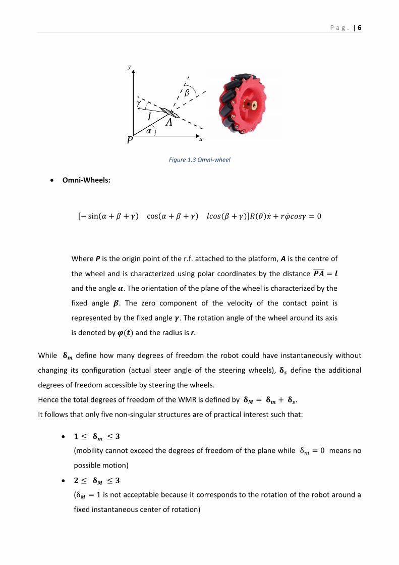
Figure 1.3 Omni-wheel

• Omni-Wheels:

[− sin(𝛼 + 𝛽 + 𝛾) cos(𝛼 + 𝛽 + 𝛾) 𝑙𝑐𝑜𝑠(𝛽 + 𝛾)]𝑅(𝜃)�̇� + 𝑟�̇�𝑐𝑜𝑠𝛾 = 0

Where P is the origin point of the r.f. attached to the platform, A is the centre of

the wheel and is characterized using polar coordinates by the distance 𝑷𝑨̅̅ ̅̅ = 𝒍

and the angle 𝜶. The orientation of the plane of the wheel is characterized by the

fixed angle 𝜷. The zero component of the velocity of the contact point is

represented by the fixed angle 𝜸. The rotation angle of the wheel around its axis

is denoted by 𝝋(𝒕) and the radius is r.

While 𝛅𝒎 define how many degrees of freedom the robot could have instantaneously without

changing its configuration (actual steer angle of the steering wheels), 𝛅𝒔 define the additional

degrees of freedom accessible by steering the wheels.

Hence the total degrees of freedom of the WMR is defined by 𝛅𝑴 = 𝛅𝒎 + 𝛅𝒔.

It follows that only five non-singular structures are of practical interest such that:

• 𝟏 ≤ 𝛅𝒎 ≤ 𝟑

(mobility cannot exceed the degrees of freedom of the plane while δ𝑚 = 0 means no

possible motion)

• 𝟐 ≤ 𝛅𝑴 ≤ 𝟑

(δ𝑀 = 1 is not acceptable because it corresponds to the rotation of the robot around a

fixed instantaneous center of rotation)

P a g . | 7

• 𝟎 ≤ 𝛅𝒔 ≤ 𝟐

These five structures present the minimum number of wheels to be classified into that category.

Every category can have obviously a bigger number of wheels, but their mobility doesn’t change,

so for the purpose of classification it has been chosen to use the simplest configuration possible

for every kind of structure.

1. 𝛅𝒎 = 𝟑, 𝛅𝒔 = 𝟎

Figure 1.4 Robot of type 3.0

Called Omnidirectional Robot, they don’t have conventional fixed or

conventional centred wheel but for example three Omni-wheels or three

conventional off-centred wheels. Such configuration gives the robot full mobility

in the plane and for the one with Omni-wheels this is achieved without any

reorientation.

P a g . | 8

2. 𝛅𝒎 = 𝟐, 𝛅𝒔 = 𝟎

Figure 1.5 Robot of type 2.0

These robots have no conventional centred orientable wheels and either one or

several conventional wheels with a single common axle. The velocity results

constrained to a two-dimensional distribution. This structure is called

“Differential Drive” and is today’s most common used among WMR due to his

simple structure and control law.

3. 𝛅𝒎 = 𝟐, 𝛅𝒔 = 𝟏

Figure 1.6 Robot of type 2.1

P a g . | 9

No conventional fixed wheel and at least one conventional centred orientable

wheel or more than one but their orientation must be coordinated to maintain

𝛅𝒔 = 𝟏. The velocity results constrained to a two-dimensional distribution.

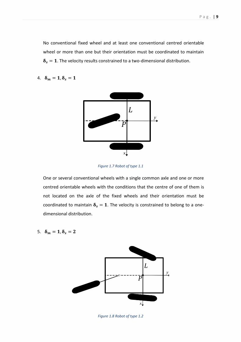
4. 𝛅𝒎 = 𝟏, 𝛅𝒔 = 𝟏

Figure 1.7 Robot of type 1.1

One or several conventional wheels with a single common axle and one or more

centred orientable wheels with the conditions that the centre of one of them is

not located on the axle of the fixed wheels and their orientation must be

coordinated to maintain 𝛅𝒔 = 𝟏. The velocity is constrained to belong to a one-

dimensional distribution.

5. 𝛅𝒎 = 𝟏, 𝛅𝒔 = 𝟐

Figure 1.8 Robot of type 1.2

P a g . | 10

No conventional fixed wheel and at least two conventional centred orientable

wheels or more but their orientation must be coordinated to maintain 𝛅𝒔 = 𝟐.

The velocity is constrained to belong to a one-dimensional distribution.

1.2 Omnidirectional and pseudo-Omnidirectional robots

For an indoor WMR is important to have 𝛅𝑴 = 𝟑 to maximize the range of movement. As seen

before it can be achieved using omni-wheels or conventional wheels. There is a third way as we

can see in (6) that “simulate” the 3 DOF. In this example the main body is linked to a differentially

driven robot platform by a revolute joint. In this way the “Head” of the WMR has full range of view

of the environment even if the platform lack of mobility in the direction orthogonal to the wheels.

For this very reason this choice is not preferable because is better having a bit more complex

structure that although bring more flexibility to the platform.

WMR with omni-wheels are called, as seen before, omnidirectional and their full mobility without

changing configuration allow to follow complex trajectory with a relatively simple mechanical

structure because there is no need of steering mechanism. On the other hand the other two

structures with 𝛅𝑴 = 𝟑 and conventional wheels are called pseudo-omnidirectional due to the

fact that they need to change their configuration (steering the wheels) to achieve full mobility.

Omnidirectional robots seems to have an advantage to pseudo-Omnidirectional ones but, as we

can see in (3), (4), (5), the usage of Omni-wheel bring to consistent posture errors due to three big

issues affecting this kind of wheel: joint velocity saturation, wheel slippage and perfect actuator

synchronization. These posture errors are of big interest because every navigation algorithm

needs to compute the WMR position by means of odometry. Hence these issues must be

addressed in order to use Omni-wheels in autonomous navigation.

This problem is overcome in (7) by using two offset steered driving wheels and two caster wheels

showing impressive Omnidirectional Mobility. The over-actuation (4 motors for 3 Dof) allows high

agility to the WMR on the plane as we can see in figure 8 but the trajectory to be planned is not

uniquely determined. Nevertheless, a not uniquely determined trajectory is useful in order to

optimize the motion of the robot.

P a g . | 11

Similar results but with a more complex structure are achieved in (8), (9), (10), (11) with the

implementation of four centred steered driving wheels on the base. Such motion strategy results

to much redundant but allows great position accuracy in order to mount a manipulator on the

robot base as we can see in (10) and (11).

1.3 Market

It is important to have a look at what offer the market nowadays in order to develop something

really innovative.

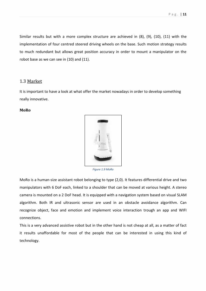
MoRo

MoRo is a human-size assistant robot belonging to type (2,0). It features differential drive and two

manipulators with 6 DoF each, linked to a shoulder that can be moved at various height. A stereo

camera is mounted on a 2 DoF head. It is equipped with a navigation system based on visual SLAM

algorithm. Both IR and ultrasonic sensor are used in an obstacle avoidance algorithm. Can

recognize object, face and emotion and implement voice interaction trough an app and WIFI

connections.

This is a very advanced assistive robot but in the other hand is not cheap at all, as a matter of fact

it results unaffordable for most of the people that can be interested in using this kind of

technology.

Figure 1.9 MoRo

P a g . | 12

Pepper

Pepper show a more anthropomorphic appearance with respect to MoRo although sharing similar

features like autonomous navigation, obstacle avoidance algorithm and WIFI and Bluetooth

connections. In a different way it doesn’t have SLAM and its shoulder are fixed but implements a

touchscreen to interact with user in fifteen different languages.

However, the main difference is the fact that it doesn’t use differential drive but 3 omnidirectional

wheels belonging to type (3,0). This structure provides a way greater navigation agility but makes

difficult internal odometry due to the slippage of the wheel.

Ipal

Five microphones are implemented on Ipal to allow sound direction detection. Its motion is based

on differential drive belongin to type (2,0) and implement two 5 DoF manipulators. It is provided

with a mono camera and a touchscreen. Like previous ones can recognize object, face and

emotions but cannot navigate autonomously, essential feature for an assistive robot. Wi-Fi and

Bluetooth are also provided.

Figure 1.10 Pepper

Figure 1.11 Ipal

P a g . | 13

Zembo

Zembo is the simplest one. Has differential drive belongin to type (2,0) and is capable of

autonomous navigation and obstacle avoidance but doesn’t have SLAM. It can recognize object

and faces and is capable of voice interaction. Is equipped with a 13 megapixels mono camera, IR

sensors, ultrasonic sensors and a touchscreen. It is capable of follow lines and moving small

objects, but it isn’t implemented with manipulators.

Figure 1.12 Asus Zembo

P a g . | 14

Chapter 2

Task analysis

It is important to perform an accurate task analysis of this robot because it will help defines the

robot structure according to what this robot must do. First of all, it must be defined the

environment where this robot will operate. This kind of robot find its natural operative

environment inside the house as a daily help, but it can be found very useful also inside offices,

workshops, laboratory, etc. as a valid assistant to the work. Considering that, the first thing that

this robot must be able to accomplish is to manage to follow people autonomously without being

of any obstacle and also to be able to deliver a service of any kind.

Inside the section 2.1 the analysis of the person follow task will be carried out, starting from

defining the various sub-tasks composing it. The choice for the various components of the robot,

both Hardware and Software, will be done according to the various requirements of the sub-tasks.

In the section 2.2 the analysis of the services task will be carried out in a similar way of the section

2.1 with the choice of the components that will results from the requirements of the various sub-

tasks.

Inside the section 2.3 it is analysed the modularity of the robot and what that concerns in terms of

structures and components.

P a g . | 15

2.1 Person follow task

Figure 2.1 Person follow sub-tasks

In order to be able to follow the user, it must detect him and autonomously navigate towards him

wherever he goes. Implementing the capability to detect human is therefore fundamental and,

moreover, could be improved by a subject locking method. Using object detection functionalities,

the robot acquires the ability to block the view on an object, it could be a necklace with led, and

recognize the user by it. Could be interesting adding the ability to recognize different users by

different necklace.

The basic hardware requirements for both human and object detection is a camera sensor. It must

be assembled in a way that could easily maintain constant visual contact with the user even in

presence of obstacle obstructing the view. To achieve this, the camera needs to be placed on top

of a telescopic pole.

From the Software point of view, a face recognition software is fundamental, as a database in

which users face will be stored.

The autonomous navigation needs primarily the SLAM (Simultaneously Localization And Mapping)

to be able to locate his position and the position of the user inside the house. Obviously, path-

planning functionalities are fundamental to allow the robot to move around. During the

movement the WMR needs to avoid unexpected obstacle as a moved chair, a person, a pet, a

cable, the stairs, etc.

P a g . | 16

In addition to the above-mentioned requirements this WMR needs the maximum degree of

manoeuvrability possible because it must be able to move around while maintaining constant

contact of view with the user. The possible structures that allow that kind of mobility are, as seen

in the section 1.1 of this thesis, the Omnidirectional one with three omni wheels and the pseudo

omnidirectional one with two steering actuated wheels and on castor wheel. Because the omni

wheels bring forth huge positioning errors due to the presence of slippage, the best choice for this

robot is the omnidirectional one that allow 3 degree of manoeuvrability and a more accurate

localization. To improve stability is recommended to put another castor wheel, so the platform will

always lay on almost three wheels during the motion.

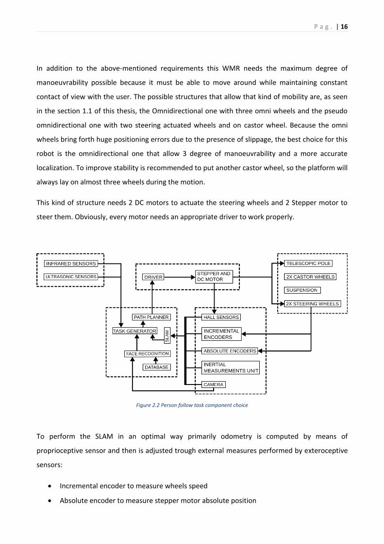
This kind of structure needs 2 DC motors to actuate the steering wheels and 2 Stepper motor to

steer them. Obviously, every motor needs an appropriate driver to work properly.

Figure 2.2 Person follow task component choice

To perform the SLAM in an optimal way primarily odometry is computed by means of

proprioceptive sensor and then is adjusted trough external measures performed by exteroceptive

sensors:

• Incremental encoder to measure wheels speed

• Absolute encoder to measure stepper motor absolute position

P a g . | 17

• Hall sensor to measure the rotor position and speed of the wheel motors

• Inertial measurements unit to measure acceleration and speed of the robot

• Camera sensor to measure distances from external reference point

Path-planning functionalities are implemented inside the microcontroller that it must be advanced

enough to manage these functionalities and the other processes of the robot. Therefore, proximity

sensors are fundamental to avoid unexpected obstacle or fall hazard:

• Ultrasonic sensors installed around the perimeter of the platform to detect big obstacles as

chair, person, walls etc.

• Infrared sensors installed near the wheels to detect the distance from the ground to avoid

the danger of falling from the stairs

A system of suspensions installed on the wheels is fundamental to avoid loss of control in

presence of small obstacle as cables on the ground due to an unstable contact wheel-floor.

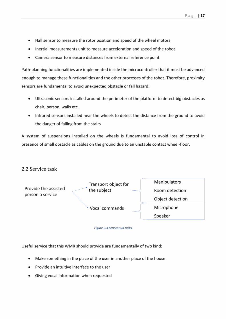
2.2 Service task

Figure 2.3 Service sub tasks

Useful service that this WMR should provide are fundamentally of two kind:

• Make something in the place of the user in another place of the house

• Provide an intuitive interface to the user

• Giving vocal information when requested

P a g . | 18

In order to be able to do something in the place of the user, the robot must be able primarily to

recognize and localize the various rooms of the house so that it could autonomously go to the

place it is asked to. To be able to do so a room detection software is essential, along with a

database collecting all the items description useful to classify every room.

After that it must be able to perform the action requested so, due to the fact that most of the task

it will be requested to do concern grabbing an object, a small but efficient manipulator is essential

along with an object detection software. The above-mentioned manipulator can be simple enough

thanks to the chosen structure: a pinch on top of an extendable pole is enough due to the high

degree of manoeuvrability of the platform.

The HMI (Human Machine Interface) is fundamental because it is the instrument by means of

which the user will be able to use this robot. If it is too much complicate and counter-intuitive the

user will not be able to use properly the robot, so it must remain simple and intuitive but in the

same time provide all the service the user will need. So beside the obvious choice of the

touchscreen a dedicated software will be ned

Figure 2.4 Service task component choice

Obviously, a microphone and a speaker are needed to give vocal information and to receive vocal

commands, as well as communicate to another person in another room in the place of the user.

P a g . | 19

Moreover, an internet connection, achievable via Wi-Fi, could be of interest to allow the WMR to

answer to the information requested from the user or even contact acquaintance.

2.3 Modularity

Another important feature for this WMR is the modularity. Even if this is not a real task that this

robot must be able to accomplish it remain still very useful to analyse because it will affect how its

mechatronic layout is structured.

Hence, the robot is splatted in two modules, one is the platform (low-level) with the motion

structure and all the sensors related to that and the other is the “head” of the robot (high-level)

with the decision-maker software, the human-machine interface and the exteroceptive sensors.

This separation allows the two modules to be fully designed autonomously and, most importantly,

to be installed with different modules depending on the work situation.

Figure 2.5 Final component choice

P a g . | 20

These two levels need to communicate between each other: a communication protocol that is

able to split completely the two level is of the outmost importance. The communication must be in

a way that even if these two modules are connected with other ones it remains the same.

P a g . | 21

Chapter 3

Kinematic analysis

In this chapter it is carried out the kinematic analysis, that is fundamental in order to understand

the motion of this robot.

In the section 3.1 the pose of the platform is defined through the definition of subsequent

reference frames. Starting from the reference frame of the chassis, the reference frames of the

wheels are defined with a recursive methodology.

In the section 3.2 is defined the generalised speed vectors of the wheels reference frames.

Following a similar recursive methodology this speed vector is defined starting from the chassis

generalized speed vector.

Inside the section 3.3 the constraint equations are analysed to obtain the relation used to describe

the motion of the robot.

In the section 3.4 the direct kinematics is analysed. The relation between the operative space and

the joint space is obtained manipulating the constraint equations.

In the section 3.5 the analysis of the inverse kinematic is carried out. At the end of the analysis

four possible configurations are defined.

The definition of the centre of instantaneous rotation is defined inside the section 3.6.

Finally, in the section 3.7, four different operative configurations are defined. Each configuration is

analysed in order to understand the various behaviour of the platform and how improve the

motion of the robot.

P a g . | 22

3.1 Pose Kinematic

Figure 3.1 Reference frames definition

The pose of the robot can be described completely by a reference frame {𝑐}, schematised in fig

(3.1). Such reference frame is completely defined through the vector 𝑝𝑐 0 = [𝑥𝑐 , 𝑦𝑐, 𝑧𝑐]

𝑇, which

defines the origin position with respect to the reference frame {0} and a 3 angles notation

(𝛼, 𝛽, 𝛾) with respect to the fixed axes 𝑥, 𝑦, 𝑧 of the reference frame {0}. Transferring such

information onto homogeneous notation (which in this document will be denoted as �̂�), the

relation (3.1.1) is obtained.

�̂�𝑐 0 = [

𝑅𝑜𝑡(𝑧, 𝛾)𝑅𝑜𝑡(𝑦, 𝛽)𝑅𝑜𝑡(𝑥, 𝛼) 𝑝𝑐 0

0𝑇 1] (3.1.1)

Making explicit the relations in equation (3.1.1) the relation (3.1.2) is obtained and by means of

that the robot pose results completely defined with respect to the fixed reference frame {0}.

�̂�𝑐 0 = [

𝑐𝛽𝑐𝛾 𝑐𝛾𝑠𝛼𝑠𝛽 − 𝑐𝛼𝑠𝛾 𝑠𝛼𝑠𝛾 + 𝑐𝛼𝑐𝛾𝑠𝛽 𝑥𝑐𝑐𝛽𝑠𝛾 𝑐𝛼𝑐𝛾 + 𝑠𝛼𝑠𝛽𝑠𝛾 𝑐𝛼𝑠𝛽𝑠𝛾 − 𝑐𝛾𝑠𝛼 𝑦𝑐−𝑠𝛽 𝑐𝛽𝑠𝛼 𝑐𝛼𝑐𝛽 𝑧𝑐0 0 0 1

] (3.1.2)

Where the abbreviated notations 𝑐𝜃 and 𝑠𝜃 stand for cos 𝜃 and sin 𝜃.

In order to define the reference frames integral with the chassis and arranged near the

attachment points of the wheels, the notation {𝑠, ~} is used where ~ sum up all four frames linked

to the wheels, identified by the subscript:

P a g . | 23

• wr: right steering actuated wheel

• wl: left steering actuated wheel

• cf: front-side castor wheel

• cb: back-side castor wheel

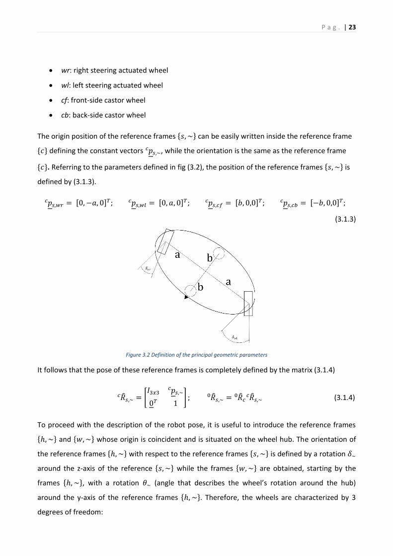
The origin position of the reference frames {𝑠, ~} can be easily written inside the reference frame

{𝑐} defining the constant vectors 𝑝𝑠,~ 𝑐 , while the orientation is the same as the reference frame

{𝑐}. Referring to the parameters defined in fig (3.2), the position of the reference frames {𝑠, ~} is

defined by (3.1.3).

𝑝𝑠,𝑤𝑟 𝑐 = [0, −𝑎, 0]𝑇; 𝑝𝑠,𝑤𝑙

𝑐 = [0, 𝑎, 0]𝑇; 𝑝𝑠,𝑐𝑓 𝑐 = [𝑏, 0,0]𝑇; 𝑝𝑠,𝑐𝑏

𝑐 = [−𝑏, 0,0]𝑇;

(3.1.3)

Figure 3.2 Definition of the principal geometric parameters

It follows that the pose of these reference frames is completely defined by the matrix (3.1.4)

�̂�𝑠,~ 𝑐 = [

𝐼3𝑥3 𝑝𝑠,~ 𝑐

0𝑇 1] ; �̂�𝑠,~

0 = �̂�𝑐 0 �̂�𝑠,~

𝑐 (3.1.4)

To proceed with the description of the robot pose, it is useful to introduce the reference frames

{ℎ, ~} and {𝑤, ~} whose origin is coincident and is situated on the wheel hub. The orientation of

the reference frames {ℎ, ~} with respect to the reference frames {𝑠, ~} is defined by a rotation 𝛿~

around the z-axis of the reference {𝑠, ~} while the frames {𝑤, ~} are obtained, starting by the

frames {ℎ, ~}, with a rotation 𝜃~ (angle that describes the wheel’s rotation around the hub)

around the y-axis of the reference frames {ℎ, ~}. Therefore, the wheels are characterized by 3

degrees of freedom:

P a g . | 24

1. A translation 𝜎~ along the z-axis of {𝑠, ~} allowed by the suspension system

2. A rotation 𝛿~ with respect to the z-axis of {𝑠, ~} allowed by the steering system

3. A rotation 𝜃~ with respect to the y-axis of {ℎ, ~} the wheel’s hub

The origin position of the reference frames {ℎ-𝑤,~} of the actuated wheels, written with respect

to the reference frames {𝑠, ~}, are reported on the relation (3.1.5).

𝑝ℎ,𝑤𝑟 𝑠,𝑤𝑟 = [0,0, 𝜎𝑤𝑟]

𝑇; 𝑝ℎ,𝑤𝑙 𝑠,𝑤𝑙 = [0, 0, 𝜎𝑤𝑙]

𝑇 (3.1.5)

To determine the origin of the reference frames {ℎ-𝑤,~} of the passive wheels it must be taken

into account of the decentralization 𝑏𝑐 along the x-axis of the reference frame {ℎ, ~} due to the

typical design of the castor wheels that guarantees the wheel’s orientation along the motion

direction. Hence, the origin position of the reference frame {ℎ-𝑤,~} of the passive wheels are

defined by the relation (3.1.6).

𝑝ℎ,𝑐𝑓 𝑠,𝑐𝑓 = [

00𝜎𝑐𝑓] + 𝑅ℎ,𝑐𝑓

𝑠,𝑐𝑓 [𝑏𝑐00] ; 𝑝ℎ,𝑐𝑏

𝑠,𝑐𝑏 = [00𝜎𝑐𝑏

] + 𝑅ℎ,𝑐𝑏 𝑠,𝑐𝑏 [

𝑏𝑐00] (3.1.6)

Where 𝑅ℎ,~ 𝑠,~ = 𝑅𝑜𝑡(𝑧, 𝛿~).

The orientation of the reference frames {ℎ, ~}, defined with respect to the reference frames

{𝑠, ~}, is a rotation around the z-axis (coincident with respect to one another) of a steering angle

𝛿~. The orientation of the reference frames {𝑤, ~}, defined with respect to the reference frames

{ℎ, ~}, is a rotation around the y-axis (coincident with respect to one another) of a wheel rotation

angle 𝜃~. Summarising, the pose of the reference frames {ℎ, ~} is defined by the homogeneous

matrix (3.1.7).

�̂�ℎ,~ 𝑠,~ = [

𝑅𝑜𝑡(𝑧, 𝛿~) 𝑝ℎ,~ 𝑠,~

0𝑇 1] ; �̂�ℎ,~

0 = �̂�𝑠,~ 0 �̂�ℎ,~

𝑠,~ (3.1.7)

The pose of the reference frames {𝑤, ~} is defined by the homogeneous matrix (3.1.8).

�̂�𝑤,~ ℎ,~ = [

𝑅𝑜𝑡(𝑧, 𝜃~) 0

0𝑇 1] ; �̂�𝑤,~

0 = �̂�ℎ,~ 0 �̂�𝑤,~

ℎ,~ (3.1.8)

P a g . | 25

By means of this recursive procedure, the definition of the reference frames used to describe the

kinematic of the robot is completed. Regarding the pose, it is left to define the contact between

the wheel and the ground.

3.1.1 Wheel-ground contact model

With an appropriate suspension system, the motion of the robot can be considered almost plane.

This consideration introduces a considerable simplification with the robot kinematic. Particularly,

it is possible to write the reference frame {𝑐} pose, with respect to the reference frame {0}, by

means of the relation (3.1.9).

�̂�𝑐 0 = [

𝑐𝛾 −𝑠𝛾 0 𝑥𝑐𝑠𝛾 𝑐𝛾 0 𝑦𝑐0 0 1 𝑧𝑐0 0 0 1

] (3.1.9)

From which it is obtained �̂�ℎ,~ 0 = �̂�𝑐

0 �̂�𝑠,~ 𝑐 �̂�ℎ,~

𝑠,~ and �̂�𝑤,~ 0 = �̂�ℎ,~

0 �̂�𝑤,~ ℎ,~ :

�̂�ℎ,𝑤𝑟 0 = [

𝑐𝛾+𝛿𝑤𝑟 −𝑠𝛾+𝛿𝑤𝑟 0 𝑥𝑐 + 𝑎𝑠𝛾𝑠𝛾+𝛿𝑤𝑟 𝑐𝛾+𝛿𝑤𝑟 0 𝑦𝑐 − 𝑎𝑐𝛾0 0 1 𝑧𝑐 + 𝜎𝑤𝑟0 0 0 1

]; �̂�ℎ,𝑤𝑙 0 = [

𝑐𝛾+𝛿𝑤𝑙 −𝑠𝛾+𝛿𝑤𝑙 0 𝑥𝑐 − 𝑎𝑠𝛾𝑠𝛾+𝛿𝑤𝑙 𝑐𝛾+𝛿𝑤𝑙 0 𝑦𝑐 + 𝑎𝑐𝛾0 0 1 𝑧𝑐 + 𝜎𝑤𝑙0 0 0 1

]

(3.1.10)

�̂�ℎ,𝑤𝑟 0 = [

𝑐𝜃𝑤𝑟𝑐𝛾+𝛿𝑤𝑟 −𝑠𝛾+𝛿𝑤𝑟 𝑠𝜃𝑤𝑟𝑐𝛾+𝛿𝑤𝑟 𝑥𝑐 + 𝑎𝑠𝛾𝑐𝜃𝑤𝑟𝑠𝛾+𝛿𝑤𝑟 𝑐𝛾+𝛿𝑤𝑟 𝑠𝜃𝑤𝑟𝑠𝛾+𝛿𝑤𝑟 𝑦𝑐 − 𝑎𝑐𝛾−𝑠𝜃𝑤𝑟 0 𝑐𝜃𝑤𝑟 𝑧𝑐 + 𝜎𝑤𝑟0 0 0 1

] ;

(3.1.11)

�̂�ℎ,𝑤𝑙 0 = [

𝑐𝜃𝑤𝑙𝑐𝛾+𝛿𝑤𝑙 −𝑠𝛾+𝛿𝑤𝑙 𝑠𝜃𝑤𝑙𝑐𝛾+𝛿𝑤𝑙 𝑥𝑐 − 𝑎𝑠𝛾𝑐𝜃𝑤𝑙𝑠𝛾+𝛿𝑤𝑙 𝑐𝛾+𝛿𝑤𝑙 𝑠𝜃𝑤𝑙𝑠𝛾+𝛿𝑤𝑙 𝑦𝑐 + 𝑎𝑐𝛾−𝑠𝜃𝑤𝑙 0 𝑐𝜃𝑤𝑙 𝑧𝑐 + 𝜎𝑤𝑙0 0 0 1

]

Through the simplification of motion almost plane, the pose of the chassis it is defined by 2

position coordinates (𝑥𝑐𝑦𝑐) and 1 rotation coordinate (𝛾). Besides, the suspensions coordinate 𝜎~

is constant, making simpler the pose of the wheel.

P a g . | 26

Figure 3.3 Definition of the reference frames for contact points

The position of the four contact points with the ground is coincident with the reference frames

{ℎ, ~} projection on the ground. Such contact points are described by the reference frames {𝑣, ~}

centered on the contact points. The orientation is easily obtained from the reference frames

{𝑤, ~} one observing that:

• The x-axis of {𝑣, ~} lies on the plane x-y of {0} and it is directed as the x projection of

{𝑤, ~}

• The z-axis of {𝑣, ~} is perpendicular to the contact plane and it is parallel to the z-axis of

{0}

In general, the projection of the vector 𝑢 on the plane 𝛼 passing through the vectors 𝑣 and 𝑤 is

given by the relation:

𝑢𝛼 = 𝑢 − 𝑢𝑛 = 𝑢 − 𝑢 ∙ 𝑛

‖𝑛‖2 𝑛

Where 𝑛 is the versor orthogonal to the plane 𝛼. On the simplified case of projection on the plane

x-y of the reference frame {0} it is obtained:

𝑢𝛼 0 = 𝑢

0 − ( 𝑢 0 ∙ 𝑘

0 ) 𝑘 0 = [

𝑢𝑥𝑢𝑦0]

Hence, it is possible to define the orientation of the reference frames integral to the contact point

by means of the relation (3.1.12).

P a g . | 27

𝑅𝑣,~ 0 =

[

𝑟11

√𝑟112 +𝑟21

2

𝑟21

√𝑟112 +𝑟21

20

𝑟21

√𝑟112 +𝑟21

2

𝑟11

√𝑟112 +𝑟21

20

0 0 1]

= [

𝑐𝛾+𝛿𝑤~ −𝑠𝛾+𝛿𝑤~ 0

𝑠𝛾+𝛿𝑤~ 𝑐𝛾+~ 0

0 0 1

] (3.1.12)

Where 𝑟𝑖𝑗 is the generic element of the matrix 𝑅𝑤,~ 0 .

Summarising, the pose of these frames, referred to the reference frame {0}, is defined by means

of the relation (3.1.13).

�̂�𝑣,𝑤𝑟 0 = [

𝑐𝛾+𝛿𝑤𝑟 −𝑠𝛾+𝛿𝑤𝑟 0 𝑥𝑐 + 𝑎𝑠𝛾𝑠𝛾+𝛿𝑤𝑟 𝑐𝛾+𝛿𝑤𝑟 0 𝑦𝑐 − 𝑎𝑐𝛾0 0 1 00 0 0 1

]; �̂�𝑣,𝑤𝑙 0 = [

𝑐𝛾+𝛿𝑤𝑙 −𝑠𝛾+𝛿𝑤𝑙 0 𝑥𝑐 − 𝑎𝑠𝛾𝑠𝛾+𝛿𝑤𝑙 𝑐𝛾+𝛿𝑤𝑙 0 𝑦𝑐 + 𝑎𝑐𝛾0 0 1 00 0 0 1

]

(3.1.13)

For future use, it is useful to obtain the rotation matrix that connect the orientation of the

reference frames {𝑣, ~} and {𝑤, ~}. Being such matrices orthonormal, the inverse is equal to the

transpose. The relations (31.14) results from that.

𝑅𝑤,~ 𝑣,~ = 𝑅𝑣,~

𝑇 0 𝑅𝑤,~

0 𝑅𝑣,~ 𝑤,~ = ( 𝑅𝑣,~

𝑇 0 𝑅𝑤,~

0 )𝑇= 𝑅𝑤,~

𝑇 0 𝑅𝑣,~

0 (3.1.14)

3.2 Velocity kinematic

The velocity of the chassis is described by the generalized speed vector:

𝑆𝑐 = [𝜔𝑐𝑣𝑐] =

[ 𝜔𝑐,𝑥𝜔𝑐,𝑦𝜔𝑐,𝑧𝑣𝑐,𝑥𝑣𝑐,𝑦𝑣𝑐,𝑧 ]

In general, such vector will be completely filled. However only the components 𝜔𝑐,𝑧 = �̇�, 𝑣𝑐,𝑥 = �̇�𝑐

and 𝑣𝑐,𝑦 = �̇�𝑐 can be controlled inside the operative space. For the purposes of motion planning it

is possible to consider null the other components, while such consideration cannot be done for

the dynamic modelling. So, it is obtained:

P a g . | 28

𝑆𝑐 =

[ 00�̇��̇�𝑐�̇�𝑐0 ]

(3.2.1)

The connection points of the suspensions are integral to the frame, so their generalized speed

vector is defined by the relation (3.2.2):

𝑆ℎ,~ = [𝜔𝑐

𝑣𝑐 + 𝜔𝑐 × 𝑅𝑐 0 𝑝ℎ,~

𝑐 ] (3.2.2)

Especially, for the actuated wheels it is obtained:

𝑆ℎ,𝑤𝑟 =

[

00�̇�

�̇�𝑐 + 𝑎�̇�𝑐𝛾�̇�𝑐 + 𝑎�̇�𝑠𝛾

0 ]

; 𝑆ℎ,𝑤𝑙 =

[

00�̇�

�̇�𝑐 − 𝑎�̇�𝑐𝛾�̇�𝑐 − 𝑎�̇�𝑠𝛾

0 ]

The hub’s velocity with respect to the connection to the frame is described by the vectors:

𝑆 ℎ,𝑤𝑟

𝑤,𝑤𝑟 =

[ 00�̇�𝑤𝑟00�̇�𝑤𝑟]

; 𝑆 ℎ,𝑤𝑙

𝑤,𝑤𝑙 =

[ 00�̇�𝑤𝑙00�̇�𝑤𝑙]

From which it is possible to write the generalize speed vector for the actuated wheels through the

relations (3.2.3).

𝑆𝑤,~ = [𝜔ℎ,~ + 𝑅ℎ,~

0 𝜔𝑤,~ ℎ,~

𝑣ℎ,~ + 𝑅ℎ,~ 0 𝑝𝑤,~

ℎ,~ ] (3.2.3)

For the purposes of motion planning it is useful considering the system as plane and without

suspension on the actuated wheels:

P a g . | 29

𝑆𝑤,𝑤𝑟 =

[

00

�̇� + �̇�𝑤𝑟�̇�𝑐 + 𝑎�̇�𝑐𝛾�̇�𝑐 + 𝑎�̇�𝑠𝛾

0 ]

; 𝑆𝑤,𝑤𝑙 =

[

00

�̇� + �̇�𝑤𝑙�̇�𝑐 − 𝑎�̇�𝑐𝛾�̇�𝑐 − 𝑎�̇�𝑠𝛾

0 ]

In general, considering the reference frame {0} and the reference frame {𝑖}, which origin is

described inside the reference frame {0} by the vector 𝑝𝑖0 and which orientation is defined by the

matrix 𝑅𝑖0 , the position of a point 𝑞 integral with the reference frame {𝑖} can be described as:

𝑝𝑞 0 = 𝑝𝑖

0 + 𝑅𝑖 0 𝑝𝑞

𝑖 ⇒ 𝑝𝑞 𝑖 = 𝑅𝑖

𝑇 0 ( 𝑝𝑞

0 − 𝑝𝑖 0 )

Deriving with respect to the time the first one and substituting the second one it is obtained:

�̇�𝑞 0 = �̇�𝑖

0 + �̇�𝑖 0 𝑅𝑖

𝑇 0 ( 𝑝𝑞

0 − 𝑝𝑖 0 )

Comparing the obtained relation with the fundamental formula of the rigid body kinematics the

equivalence (3.2.4) is obtained.

�̇�𝑖 0 𝑅𝑖

𝑇 0 = 𝜔𝑖

0 × (3.2.4)

Such relation is useful for the computation of the angular velocity vector of a reference frame

starting from its orientation matrix.

Applying the relation (3.2.4) to the reference frames integral with the contact area it is obtained:

𝜔𝑣,~ × = �̇�𝑣,~ 0 𝑅𝑣,~

𝑇 0 (3.2.5)

In the case of plain motion can be written as:

𝜔𝑣,𝑤𝑟 = [00

�̇� + �̇�𝑤𝑟

]; 𝜔𝑣,𝑤𝑙 = [

00

�̇� + �̇�𝑤𝑙

]

In order to obtain the velocity of the reference frames {𝑣, ~} it is possible to write:

�̇�𝑣,~ 0 =

𝑑

𝑑𝑡( 𝑝𝑣,~ 0 ) =

𝑑

𝑑𝑡( 𝑝𝑤,~ 0 + 𝑅𝑤,~

0 𝑝𝑣,~ 𝑤,~ ) (3.2.6)

From the equation (3.2.6) it is obtained:

P a g . | 30

𝑝𝑣,~ 𝑤,~ = 𝑅𝑤,~

𝑇 0 ( 𝑝𝑣,~

0 − 𝑝𝑤,~ 0 ) (3.2.7)

Making explicit the derivative of the equation (3.2.6) e substituting the relation (3.2.7), the

relation is obtained:

�̇�𝑣,~ 0 = �̇�𝑤,~

0 + �̇�𝑤,~ 0 ( 𝑝𝑣,~

0 − 𝑝𝑤,~ 0 ) = �̇�𝑤,~

0 + �̇�𝑤,~ 0 𝑅𝑤,~

𝑇 0 ( 𝑝𝑣,~

0 − 𝑝𝑤,~ 0 ) (3.2.8)

Deriving the position vectors of the reference frame {𝑤, ~} with respect to the time, the linear

speed expressed by the relations (3.2.9) are obtained.

�̇� 0𝑤,𝑤𝑟 = [

�̇�𝑐 + 𝑎�̇�𝑐𝛾�̇�𝑐 + 𝑎�̇�𝑠𝛾

0

]; �̇� 0𝑤,𝑤𝑙 = [

�̇�𝑐 − 𝑎�̇�𝑐𝛾�̇�𝑐 − 𝑎�̇�𝑠𝛾

0

] (3.2.9)

Making explicit the product �̇�𝑤,~ 0 𝑅𝑤,~

𝑇 0 the relation (3.2.10) is obtained.

�̇�𝑤,~ 0 𝑅𝑤,~

𝑇 0 ( 𝑝𝑣,~

0 − 𝑝𝑤,~ 0 ) = �̇�~ [

0 0 𝑐𝛾+𝛿~0 0 𝑠𝛾+𝛿~

−𝑐𝛾+𝛿~ −𝑠𝛾+𝛿~ 0] [

00−𝑟𝑤

] = [

−𝑟𝑤�̇�~𝑐𝛾+𝛿~−𝑟𝑤�̇�~𝑠𝛾+𝛿~

0

]

(3.2.10)

Summarizing, the generalize speed vectors associated with the reference frames {𝑣, ~} are

defined by the relation (3.2.11).

𝑆𝑣,𝑤𝑟 =

[

00

�̇� + �̇�𝑤𝑟�̇�𝑐 + 𝑎�̇�𝑐𝛾 − 𝑟𝑤�̇�𝑤𝑟𝑐𝛾+𝛿𝑤𝑟�̇�𝑐 + 𝑎�̇�𝑠𝛾 − 𝑟𝑤�̇�𝑤𝑟𝑠𝛾+𝛿𝑤𝑟

0 ]

; 𝑆𝑣,𝑤𝑙 =

[

00

�̇� + �̇�𝑤𝑙�̇�𝑐 − 𝑎�̇�𝑐𝛾 − 𝑟𝑤�̇�𝑤𝑙𝑐𝛾+𝛿𝑤𝑙�̇�𝑐 − 𝑎�̇�𝑠𝛾 − 𝑟𝑤�̇�𝑤𝑙𝑠𝛾+𝛿𝑤𝑙

0 ]

(3.2.11)

3.3 Constraint equations

In order to respect the pure rolling constraint, the velocity of the contact point must be equal to

zero. The constraint on the passive wheels is not useful to the motion planning, while the

constraint equation obtained imposing the constraint on the actuated wheels are relevant. Such

constraint is translated in a set of 3 equations for every wheel as:

P a g . | 31

�̇�𝑣,~ 0 = 0 (3.3.1)

Considering the expressions defined on the equation (3.2.11), the constraint equation (3.3.1), for

the two actuated wheels, can be written in the shape (3.3.2).

{

�̇�𝑐 + 𝑎�̇�𝑐𝛾 − 𝑟𝑤�̇�𝑤𝑟𝑐𝛾+𝛿𝑤𝑟 = 0; (𝑎)

�̇�𝑐 + 𝑎�̇�𝑠𝛾 − 𝑟𝑤�̇�𝑤𝑟𝑠𝛾+𝛿𝑤𝑟 = 0; (𝑏)

�̇�𝑐 − 𝑎�̇�𝑐𝛾 − 𝑟𝑤�̇�𝑤𝑙𝑐𝛾+𝛿𝑤𝑙 = 0; (𝑐)

�̇�𝑐 − 𝑎�̇�𝑠𝛾 − 𝑟𝑤�̇�𝑤𝑙𝑠𝛾+𝛿𝑤𝑙 = 0; (𝑑)

⇔ 𝛷 =

[ �̇�𝑐 + 𝑎�̇�𝑐𝛾 − 𝑟𝑤�̇�𝑤𝑟𝑐𝛾+𝛿𝑤𝑟�̇�𝑐 + 𝑎�̇�𝑠𝛾 − 𝑟𝑤�̇�𝑤𝑟𝑠𝛾+𝛿𝑤𝑟�̇�𝑐 − 𝑎�̇�𝑐𝛾 − 𝑟𝑤�̇�𝑤𝑙𝑐𝛾+𝛿𝑤𝑙�̇�𝑐 − 𝑎�̇�𝑠𝛾 − 𝑟𝑤�̇�𝑤𝑙𝑠𝛾+𝛿𝑤𝑙 ]

= 0

(3.3.2)

From this set of constraint equation, it is possible to obtain a relation useful to understand the

true manoeuvrability of the robot. Particularly, subtracting to the equations (3.3.2)(a) and

(3.3.2)(b) the equations (3.3.2)(c) and (3.3.2)(d) the equations are obtained:

(𝑎) − (𝑐) ⇒ 2𝑎�̇� = 𝑟𝑤(�̇�𝑤𝑟𝑐𝛿𝑤𝑟 − �̇�𝑤𝑙𝑐𝛿𝑤𝑙) − 𝑟𝑤𝑠𝛾

𝑐𝛾(�̇�𝑤𝑟𝑠𝛿𝑤𝑟 − �̇�𝑤𝑙𝑠𝛿𝑤𝑙)

(𝑏) − (𝑑) ⇒ 2𝑎�̇� = 𝑟𝑤(�̇�𝑤𝑟𝑐𝛿𝑤𝑟 − �̇�𝑤𝑙𝑐𝛿𝑤𝑙) − 𝑟𝑤𝑐𝛾

𝑠𝛾(�̇�𝑤𝑟𝑠𝛿𝑤𝑟 − �̇�𝑤𝑙𝑠𝛿𝑤𝑙)

From which the wanted relation (3.3.3) is obtained.

�̇�𝑤𝑟𝑠𝛿𝑤𝑟 = �̇�𝑤𝑙𝑠𝛿𝑤𝑙 (3.3.3)

It is important to notice that the relation (3.3.3) is always verified when 𝛿𝑤𝑟 and 𝛿𝑤𝑙 are equal to

zero, while imposes a constraint on the assignment of the angular speeds of the two wheels on

the others configurations.

3.4 Direct Kinematics

Being the system over actuated, the four constraint equation are over abundant for the means of

the computation of the platform speeds inside the operative space given a joint space velocity set.

It follows that a relation between the joint space speeds must exists. Such relation (equation

(3.3.3)) is already obtained inside the section 3.3.

P a g . | 32

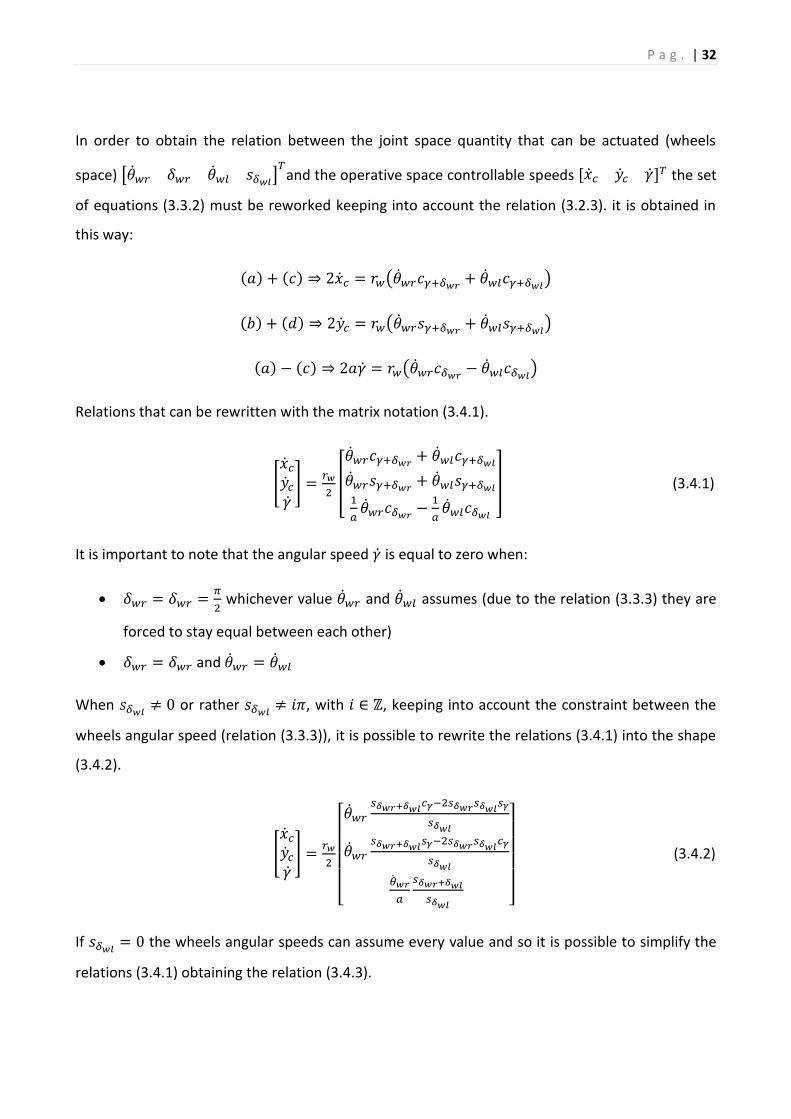
In order to obtain the relation between the joint space quantity that can be actuated (wheels

space) [�̇�𝑤𝑟 𝛿𝑤𝑟 �̇�𝑤𝑙 𝑠𝛿𝑤𝑙]𝑇

and the operative space controllable speeds [�̇�𝑐 �̇�𝑐 �̇�]𝑇 the set

of equations (3.3.2) must be reworked keeping into account the relation (3.2.3). it is obtained in

this way:

(𝑎) + (𝑐) ⇒ 2�̇�𝑐 = 𝑟𝑤(�̇�𝑤𝑟𝑐𝛾+𝛿𝑤𝑟 + �̇�𝑤𝑙𝑐𝛾+𝛿𝑤𝑙)

(𝑏) + (𝑑) ⇒ 2�̇�𝑐 = 𝑟𝑤(�̇�𝑤𝑟𝑠𝛾+𝛿𝑤𝑟 + �̇�𝑤𝑙𝑠𝛾+𝛿𝑤𝑙)

(𝑎) − (𝑐) ⇒ 2𝑎�̇� = 𝑟𝑤(�̇�𝑤𝑟𝑐𝛿𝑤𝑟 − �̇�𝑤𝑙𝑐𝛿𝑤𝑙)

Relations that can be rewritten with the matrix notation (3.4.1).

[�̇�𝑐�̇�𝑐�̇�] =

𝑟𝑤

2[

�̇�𝑤𝑟𝑐𝛾+𝛿𝑤𝑟 + �̇�𝑤𝑙𝑐𝛾+𝛿𝑤𝑙�̇�𝑤𝑟𝑠𝛾+𝛿𝑤𝑟 + �̇�𝑤𝑙𝑠𝛾+𝛿𝑤𝑙1

𝑎�̇�𝑤𝑟𝑐𝛿𝑤𝑟 −

1

𝑎�̇�𝑤𝑙𝑐𝛿𝑤𝑙

] (3.4.1)

It is important to note that the angular speed �̇� is equal to zero when:

• 𝛿𝑤𝑟 = 𝛿𝑤𝑟 =𝜋

2 whichever value �̇�𝑤𝑟 and �̇�𝑤𝑙 assumes (due to the relation (3.3.3) they are

forced to stay equal between each other)

• 𝛿𝑤𝑟 = 𝛿𝑤𝑟 and �̇�𝑤𝑟 = �̇�𝑤𝑙

When 𝑠𝛿𝑤𝑙 ≠ 0 or rather 𝑠𝛿𝑤𝑙 ≠ 𝑖𝜋, with 𝑖 ∈ ℤ, keeping into account the constraint between the

wheels angular speed (relation (3.3.3)), it is possible to rewrite the relations (3.4.1) into the shape

(3.4.2).

[�̇�𝑐�̇�𝑐�̇�] =

𝑟𝑤

2

[ �̇�𝑤𝑟

𝑠𝛿𝑤𝑟+𝛿𝑤𝑙𝑐𝛾−2𝑠𝛿𝑤𝑟𝑠𝛿𝑤𝑙𝑠𝛾

𝑠𝛿𝑤𝑙

�̇�𝑤𝑟𝑠𝛿𝑤𝑟+𝛿𝑤𝑙𝑠𝛾−2𝑠𝛿𝑤𝑟𝑠𝛿𝑤𝑙𝑐𝛾

𝑠𝛿𝑤𝑙

�̇�𝑤𝑟

𝑎

𝑠𝛿𝑤𝑟+𝛿𝑤𝑙

𝑠𝛿𝑤𝑙 ]

(3.4.2)

If 𝑠𝛿𝑤𝑙 = 0 the wheels angular speeds can assume every value and so it is possible to simplify the

relations (3.4.1) obtaining the relation (3.4.3).

P a g . | 33

[�̇�𝑐�̇�𝑐�̇�] =

𝑟𝑤

2[

�̇�𝑤𝑟𝑐𝛾+𝛿𝑤𝑟 ± �̇�𝑤𝑙𝑐𝛾

�̇�𝑤𝑟𝑠𝛾+𝛿𝑤𝑟 ± �̇�𝑤𝑙𝑐𝛾1

𝑎�̇�𝑤𝑟𝑐𝛿𝑤𝑟 ∓

1

𝑎�̇�𝑤𝑙

] (3.4.3)

3.5 Inverse kinematics

To obtain a solution to the inverse kinematic problem (relation that allow to go from the operative

space to the joint space) it is possible to work on the constraint relations (equation (3.3.2)) as

follows:

(𝑎)2 + (𝑏)2 ⇒ (�̇�𝑐 + 𝑎�̇�𝑐𝛾)2+ (�̇�𝑐 + 𝑎�̇�𝑠𝛾)

2= 𝑟𝑤

2�̇�𝑤𝑟2 (𝑐𝛾+𝛿𝑤𝑟

2 + 𝑠𝛾+𝛿𝑤𝑟2 ) = 𝑟𝑤

2�̇�𝑤𝑟2

(𝑐)2 + (𝑑)2 ⇒ (�̇�𝑐 − 𝑎�̇�𝑐𝛾)2+ (�̇�𝑐 − 𝑎�̇�𝑠𝛾)

2= 𝑟𝑤

2�̇�𝑤𝑙2 (𝑐𝛾+𝛿𝑤𝑙

2 + 𝑠𝛾+𝛿𝑤𝑙2 ) = 𝑟𝑤

2�̇�𝑤𝑙2

From which the relation (3.5.1) is obtained.

�̇�𝑤𝑟 = ±1

𝑟𝑤√(�̇�𝑐 + 𝑎�̇�𝑐𝛾)

2+ (�̇�𝑐 + 𝑎�̇�𝑠𝛾)

2

(3.5.1)

�̇�𝑤𝑙 = ±1

𝑟𝑤√(�̇�𝑐 − 𝑎�̇�𝑐𝛾)

2+ (�̇�𝑐 − 𝑎�̇�𝑠𝛾)

2

The laws for the variables 𝛿~ will only be obtained for the right wheel, however similar relation

can be obtained for the left one, of which only the result will be shown. The relations (3.3.2)(a)

and (3.3.2)(b) can be rewritten, using the parametric formulas of sin and cosine, into the shape:

�̇�𝑐 + 𝑎�̇�𝑐𝛾 = 𝑟𝑤�̇�𝑤𝑟𝑐𝛾+𝛿𝑤𝑟 = 𝑟𝑤�̇�𝑤𝑟1 − 𝑡2

1 + 𝑡2 (𝑒)

�̇�𝑐 + 𝑎�̇�𝑠𝛾 = 𝑟𝑤�̇�𝑤𝑟𝑠𝛾+𝛿𝑤𝑟 = 𝑟𝑤�̇�𝑤𝑟2𝑡

1 + 𝑡2 (𝑓)

Where 𝑡 = 𝑡𝑎𝑛𝛾+𝛿𝑤𝑟

2 with 𝛾 + 𝛿𝑤𝑟 ≠ 𝜋 + 2𝑘𝜋, with 𝑘 ∈ ℤ.

Obtaining (𝑖 + 𝑡2) from (f) and substituting that in (e) the second-grade equation on 𝑡 is obtained:

𝑡2 +�̇�𝑐 + 𝑎�̇�𝑐𝛾

�̇�𝑐 + 𝑎�̇�𝑠𝛾2𝑡 + 1 = 0 ⇒ 𝑡 = −

�̇�𝑐 + 𝑎�̇�𝑐𝛾

�̇�𝑐 + 𝑎�̇�𝑠𝛾±√(

�̇�𝑐 + 𝑎�̇�𝑐𝛾

�̇�𝑐 + 𝑎�̇�𝑠𝛾)

2

+ 1

P a g . | 34

From this relation the solutions shown into the equation (3.5.2) are obtained.

𝛿𝑤𝑟 = −𝛾 − 2𝑎𝑟𝑐𝑡𝑎𝑛(�̇�𝑐 + 𝑎�̇�𝑐𝛾

�̇�𝑐 + 𝑎�̇�𝑠𝛾∓√(

�̇�𝑐 + 𝑎�̇�𝑐𝛾

�̇�𝑐 + 𝑎�̇�𝑠𝛾)

2

+ 1) = −𝛾 − 2𝑎𝑟𝑐𝑡𝑎𝑛 (�̇�𝑐 + 𝑎�̇�𝑐𝛾

�̇�𝑐 + 𝑎�̇�𝑠𝛾−

𝑟𝑤�̇�𝑤𝑟�̇�𝑐 + 𝑎�̇�𝑠𝛾

)

(3.5.2)

Similarly, the two solutions (3.5.3) are obtained.

𝛿𝑤𝑙 = −𝛾 − 2𝑎𝑟𝑐𝑡𝑎𝑛(�̇�𝑐 − 𝑎�̇�𝑐𝛾

�̇�𝑐 − 𝑎�̇�𝑠𝛾∓√(

�̇�𝑐 − 𝑎�̇�𝑐𝛾

�̇�𝑐 − 𝑎�̇�𝑠𝛾)

2

+ 1) = −𝛾 − 2𝑎𝑟𝑐𝑡𝑎𝑛 (�̇�𝑐 − 𝑎�̇�𝑐𝛾

�̇�𝑐 − 𝑎�̇�𝑠𝛾−

𝑟𝑤�̇�𝑤𝑙�̇�𝑐 − 𝑎�̇�𝑠𝛾

)

(3.5.3)

In relation to the equations (3.5.1), (3.5.2) and (3.5.3), it can be seen that the relations for the

right wheel and for the left wheel provide two independent solutions for each wheel. It follows

that the inverse kinematics problem of the platform allows 4 possible configurations, defined by

the relations shown into the equation (3.5.4).

𝐈 =

[ �̇�𝑤𝑟 = +

1

𝑟𝑤√(�̇�𝑐 + 𝑎�̇�𝑐𝛾)

2+ (�̇�𝑐 + 𝑎�̇�𝑠𝛾)

2

𝛿𝑤𝑟 = −𝛾 − 2𝑎𝑟𝑐𝑡𝑎𝑛(�̇�𝑐+𝑎�̇�𝑐𝛾

�̇�𝑐+𝑎�̇�𝑠𝛾−√(

�̇�𝑐+𝑎�̇�𝑐𝛾

�̇�𝑐+𝑎�̇�𝑠𝛾)2

+ 1)

�̇�𝑤𝑙 = +1

𝑟𝑤√(�̇�𝑐 − 𝑎�̇�𝑐𝛾)

2+ (�̇�𝑐 − 𝑎�̇�𝑠𝛾)

2

𝛿𝑤𝑙 = −𝛾 − 2𝑎𝑟𝑐𝑡𝑎𝑛(�̇�𝑐−𝑎�̇�𝑐𝛾

�̇�𝑐−𝑎�̇�𝑠𝛾−√(

�̇�𝑐−𝑎�̇�𝑐𝛾

�̇�𝑐−𝑎�̇�𝑠𝛾)2

+ 1)

]

;

𝐈𝐈 =

[ �̇�𝑤𝑟 = −

1

𝑟𝑤√(�̇�𝑐 + 𝑎�̇�𝑐𝛾)

2+ (�̇�𝑐 + 𝑎�̇�𝑠𝛾)

2

𝛿𝑤𝑟 = −𝛾 − 2𝑎𝑟𝑐𝑡𝑎𝑛 (�̇�𝑐+𝑎�̇�𝑐𝛾

�̇�𝑐+𝑎�̇�𝑠𝛾+√(

�̇�𝑐+𝑎�̇�𝑐𝛾

�̇�𝑐+𝑎�̇�𝑠𝛾)2

+ 1)

�̇�𝑤𝑙 = +1

𝑟𝑤√(�̇�𝑐 − 𝑎�̇�𝑐𝛾)

2+ (�̇�𝑐 − 𝑎�̇�𝑠𝛾)

2

𝛿𝑤𝑙 = −𝛾 − 2𝑎𝑟𝑐𝑡𝑎𝑛 (�̇�𝑐−𝑎�̇�𝑐𝛾

�̇�𝑐−𝑎�̇�𝑠𝛾−√(

�̇�𝑐−𝑎�̇�𝑐𝛾

�̇�𝑐−𝑎�̇�𝑠𝛾)2

+ 1)

]

;

(3.5.4)

P a g . | 35

𝐈𝐈𝐈 =

[ �̇�𝑤𝑟 = +

1

𝑟𝑤√(�̇�𝑐 + 𝑎�̇�𝑐𝛾)

2+ (�̇�𝑐 + 𝑎�̇�𝑠𝛾)

2

𝛿𝑤𝑟 = −𝛾 − 2𝑎𝑟𝑐𝑡𝑎𝑛(�̇�𝑐+𝑎�̇�𝑐𝛾

�̇�𝑐+𝑎�̇�𝑠𝛾−√(

�̇�𝑐+𝑎�̇�𝑐𝛾

�̇�𝑐+𝑎�̇�𝑠𝛾)2

+ 1)

�̇�𝑤𝑙 = −1

𝑟𝑤√(�̇�𝑐 − 𝑎�̇�𝑐𝛾)

2+ (�̇�𝑐 − 𝑎�̇�𝑠𝛾)

2

𝛿𝑤𝑙 = −𝛾 − 2𝑎𝑟𝑐𝑡𝑎𝑛 (�̇�𝑐−𝑎�̇�𝑐𝛾

�̇�𝑐−𝑎�̇�𝑠𝛾+√(

�̇�𝑐−𝑎�̇�𝑐𝛾

�̇�𝑐−𝑎�̇�𝑠𝛾)2

+ 1)

]

;

𝐈𝐕 =

[ �̇�𝑤𝑟 = −

1

𝑟𝑤√(�̇�𝑐 + 𝑎�̇�𝑐𝛾)

2+ (�̇�𝑐 + 𝑎�̇�𝑠𝛾)

2

𝛿𝑤𝑟 = −𝛾 − 2𝑎𝑟𝑐𝑡𝑎𝑛 (�̇�𝑐+𝑎�̇�𝑐𝛾

�̇�𝑐+𝑎�̇�𝑠𝛾+√(

�̇�𝑐+𝑎�̇�𝑐𝛾

�̇�𝑐+𝑎�̇�𝑠𝛾)2

+ 1)

�̇�𝑤𝑙 = −1

𝑟𝑤√(�̇�𝑐 − 𝑎�̇�𝑐𝛾)

2+ (�̇�𝑐 − 𝑎�̇�𝑠𝛾)

2

𝛿𝑤𝑙 = −𝛾 − 2𝑎𝑟𝑐𝑡𝑎𝑛 (�̇�𝑐−𝑎�̇�𝑐𝛾

�̇�𝑐−𝑎�̇�𝑠𝛾+√(

�̇�𝑐−𝑎�̇�𝑐𝛾

�̇�𝑐−𝑎�̇�𝑠𝛾)2

+ 1)

]

;

3.6 Centre of instantaneous rotation

Geometrically, the centre of instantaneous rotation 𝐼𝑐𝑟 is located at the intersection of the

projection of the wheels rotation axes on the motion plane 𝑧 = 0. The projection of the wheels

rotation axes are located along the y-axis of the reference frames {𝑣, ~}. It follows that these lines

can be described by the relations:

𝜌𝑤𝑟: 𝜆1 𝑅𝑣,𝑤𝑟 0 𝑗 + 𝑝𝑣,𝑤𝑟

0 ; 𝜌𝑤𝑙: 𝜆2 𝑅𝑣,𝑤𝑙 0 𝑗 + 𝑝𝑣,𝑤𝑙

0 ;

From the which the system of equations is obtained:

𝜆1 [

−𝑠𝛾+𝛿𝑤𝑟𝑐𝛾+𝛿𝑤𝑟0

] + [𝑥𝑐 + 𝑎𝑠𝛾𝑦𝑐 − 𝑎𝑐𝛾

0

] = 𝜆2 [

−𝑠𝛾+𝛿𝑤𝑙𝑐𝛾+𝛿𝑤𝑙0

] + [

𝑥𝑐 − 𝑎𝑠𝛾𝑦𝑐 + 𝑎𝑐𝛾

0]

The expressions are obtained solving such system:

P a g . | 36

𝜆1 = 2𝑎𝑠𝛿𝑤𝑙

𝑠𝛿𝑤𝑙−𝛿𝑤𝑟 𝜆1 = 2𝑎

𝑠𝛿𝑤𝑟𝑠𝛿𝑤𝑙−𝛿𝑤𝑟

Once these relations are known, the centre of instantaneous rotation can be computed by means

of the relation (3.6.1).

𝐼𝑐𝑟 = 𝜆1 [

−𝑠𝛾+𝛿𝑤𝑟𝑐𝛾+𝛿𝑤𝑟0

] + [𝑥𝑐 + 𝑎𝑠𝛾𝑦𝑐 − 𝑎𝑐𝛾

0

] =

[ 𝑎

𝑠𝛿𝑤𝑙𝑠𝛾+𝛿𝑤𝑟+𝑠𝛿𝑤𝑟𝑠𝛾+𝛿𝑤𝑙

𝑠𝛿𝑤𝑙−𝛿𝑤𝑟+ 𝑥𝑐

𝑎𝑠𝛿𝑤𝑙𝑐𝛾+𝛿𝑤𝑟+𝑠𝛿𝑤𝑟𝑐𝛾+𝛿𝑤𝑙

𝑠𝛿𝑤𝑙−𝛿𝑤𝑟+ 𝑦𝑐

0 ]

(3.6.1)

With this formula it is not possible to compute the centre of instantaneous rotation when 𝛿𝑤𝑟 =

𝛿𝑤𝑙, condition that happen when the wheels are parallel with respect to each other. In such

configuration it is possible to write:

𝑣𝑐 = [00�̇�] × (𝑝𝑐 − 𝐼𝑐𝑟) = [

−�̇�(𝑦𝑐 − 𝐼𝑐𝑟,𝑦)

�̇�(𝑥𝑐 − 𝐼𝑐𝑟,𝑥)

0

]

From which the relation (3.6.2) is obtained. Such relation is useful for the computation of the

centre of instantaneous rotation under the condition of 𝛿𝑤𝑟 = 𝛿𝑤𝑙.

𝐼𝑐𝑟 = [

𝑥𝑐 −𝑣𝑐,𝑦

�̇�

𝑦𝑐 +𝑣𝑐,𝑥

�̇�

0

] (3.6.2)

The problem is obviously singular for �̇� = 0.

3.7 Operative configurations

The ways the robot can move can be divided in four different steering configurations, schematized

in fig (3.4).

P a g . | 37

Figure 3.4 Operative configurations

Configuration I 𝛿𝑤𝑟 ≠ 𝛿𝑤𝑙. This case represents the most general configuration obtainable, with

which the robot can use every grade of mobility to obtain any motion on the plane. The position of

the centre of instantaneous rotation is computed with the formula (3.6.1).

Configuration II 𝛿𝑤𝑟 = 𝛿𝑤𝑙 ≠ 0, 𝜋 2⁄ . In this configuration the wheels axes are parallel but not

coincident. This configuration allows the robot to translate but not to rotate. As a matter of fact,

the equation (3.3.3) impose that the wheels angular speeds must be equal: �̇�𝑤𝑟 = �̇�𝑤𝑙 . This kind of

configuration can be used, during the person follow task, to maintain a fixed direction of view

while translating on the plane.

Configuration III 𝛿𝑤𝑟 = 𝛿𝑤𝑙 = 0. This configuration is the classic differential drive: coincident

wheels axes. The constraint equation (3.3.3) is always satisfied for any angular speed of the

wheels. The position of the centre of instantaneous rotation can be computed with the relation

(3.6.2) and it is located on the y-axis of the reference frame {𝑐}. It follows that the robot can have

angular speed, but it loses the possibility to actuate a velocity along the y-axis of {𝑐}. Such

configuration is useful to maintain the centripetal acceleration of the chassis, during curvilinear

motion, on the y-axis of {𝑐}.

Configuration IV 𝛿𝑤𝑟 = 𝛿𝑤𝑙 =𝜋2⁄ . In this configuration, the wheels angular speed must be the

same due to the constraint relation (3.3.3) and the wheels axes are parallel, but not coincident.

However, this configuration has interesting characteristic from the static and dynamic point of

view.

The distances between the two actuated wheels and the two passive wheels are different in order

to allow the platform to move into a space built for the humans and filled with obstacle. The robot

acceleration around a vertical axis is tied to the capability of its actuators to develop torque

P a g . | 38

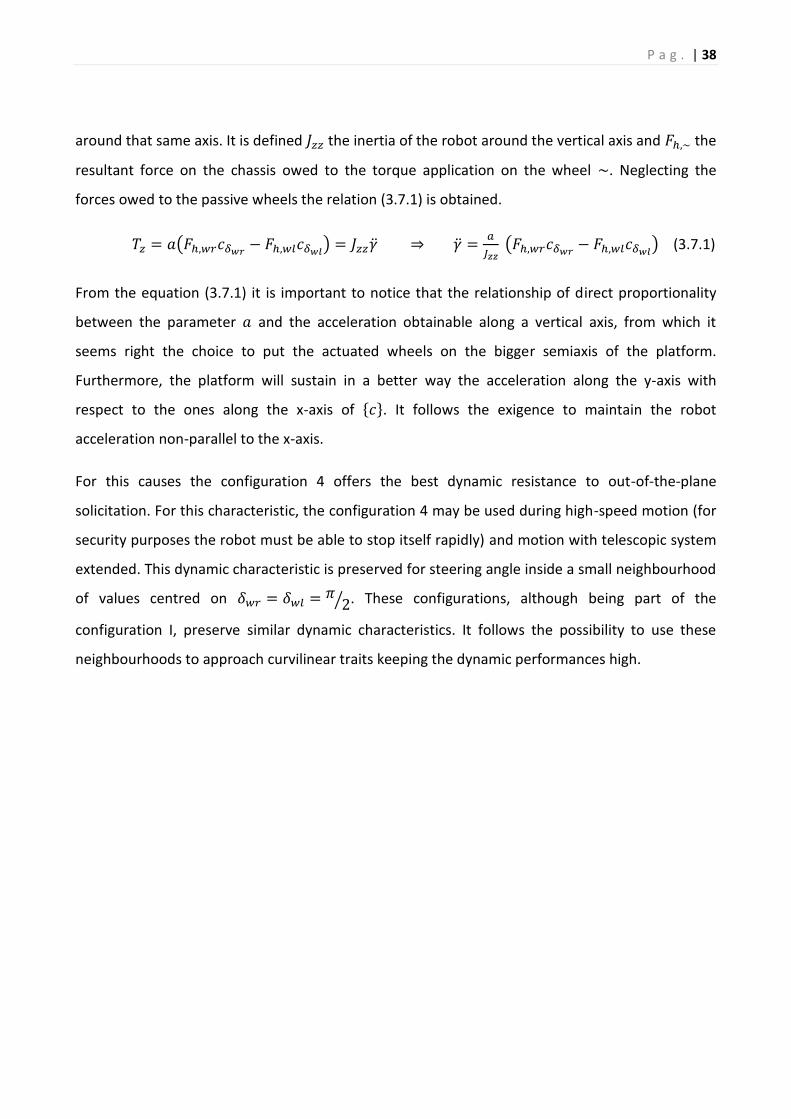
around that same axis. It is defined 𝐽𝑧𝑧 the inertia of the robot around the vertical axis and 𝐹ℎ,~ the

resultant force on the chassis owed to the torque application on the wheel ~. Neglecting the

forces owed to the passive wheels the relation (3.7.1) is obtained.

𝑇𝑧 = 𝑎(𝐹ℎ,𝑤𝑟𝑐𝛿𝑤𝑟 − 𝐹ℎ,𝑤𝑙𝑐𝛿𝑤𝑙) = 𝐽𝑧𝑧�̈� ⇒ �̈� =𝑎

𝐽𝑧𝑧 (𝐹ℎ,𝑤𝑟𝑐𝛿𝑤𝑟 − 𝐹ℎ,𝑤𝑙𝑐𝛿𝑤𝑙) (3.7.1)

From the equation (3.7.1) it is important to notice that the relationship of direct proportionality

between the parameter 𝑎 and the acceleration obtainable along a vertical axis, from which it

seems right the choice to put the actuated wheels on the bigger semiaxis of the platform.

Furthermore, the platform will sustain in a better way the acceleration along the y-axis with

respect to the ones along the x-axis of {𝑐}. It follows the exigence to maintain the robot

acceleration non-parallel to the x-axis.

For this causes the configuration 4 offers the best dynamic resistance to out-of-the-plane

solicitation. For this characteristic, the configuration 4 may be used during high-speed motion (for

security purposes the robot must be able to stop itself rapidly) and motion with telescopic system

extended. This dynamic characteristic is preserved for steering angle inside a small neighbourhood

of values centred on 𝛿𝑤𝑟 = 𝛿𝑤𝑙 =𝜋2⁄ . These configurations, although being part of the

configuration I, preserve similar dynamic characteristics. It follows the possibility to use these

neighbourhoods to approach curvilinear traits keeping the dynamic performances high.

P a g . | 39

Chapter 4

Trajectory planning

In this chapter is analysed how to develop an optimised method to plan the trajectory for this

robot. The trajectory can be defined inside the operative space or inside the joint space, but in the

case of a WMR is preferrable to define it inside the operative space to actually control how and

where the robot travels inside the workspace. A trajectory inside the operative space is composed

by a geometric path, that defines where the robot moves inside the space, and a law of motion

that defines how the robot travel along the above-mentioned geometric path.

The parametric definition of the geometric trajectory is carried out inside the section 4.1, first

using straight lines and then with Bezier polynomials.

The definition of the motion law is analysed inside the chapter 4.2 for both position and

orientation.

4.1 Parametric definition of the geometric trajectory

The most intuitive way to travel inside the operative space from a point A to a point B is with a

straight line connecting the various point. Using a parameter 𝑘 defined inside the interval 0 ≤ 𝑘 ≤

1, the generic point 𝑋 is located on the segment as:

𝑝𝑋 − 𝑝𝐴 = 𝑘 (𝑝𝐵 − 𝑝𝐴)

From which it is obtained the parametric expression of the straight line:

𝑝𝑋 = (1 − 𝑘)𝑝𝐴 + 𝑘𝑝𝐵 𝑤𝑖𝑡ℎ 0 ≤ 𝑘 ≤ 1 (4.1.1)

P a g . | 40

Deriving the equation (4.1.1) the vectors are obtained:

𝑑

𝑑𝑘(𝑝𝑋) = (𝑝𝐵 − 𝑝𝐴) ;

𝑑2

𝑑𝑘2(𝑝𝑋) = 0

This method appears too rigid because doesn’t allow to specify the directions of the tangents on

the initial and final points.

However, the straight lines are very useful to defines the parametric variation of the 𝛾:

𝛾𝑋 = (1 − 𝑘)𝛾𝐴 + 𝑘𝛾𝐵 𝑤𝑖𝑡ℎ 0 ≤ 𝑘 ≤ 1 (4.1.2)

From which is obtained:

𝑑

𝑑𝑘(𝛾𝑋) = (𝛾𝐵 − 𝛾𝐴);

𝑑2

𝑑𝑘2(𝛾𝑋) = 0

Using the Bézier polynomials is possible to define parametrically a geometric trajectory between

two points through the definition of control points.

Figure 4.1 Bézier curve with one control point

Considering the figure 4.1, A and C are connected between each other with a regular curve

tangent in A to the line AB and tangent in C to the line BC. The generic point 𝑋1 is located on the

P a g . | 41

segment AB and is defined parametrically, using as before the parameter 𝑘 defined inside the

interval 0 ≤ 𝑘 ≤ 1, as:

𝑝𝑋1 − 𝑝𝐴 = 𝑘 (𝑝𝐵 − 𝑝𝐴) ⇔ 𝑝𝑋1 = (1 − 𝑘)𝑝𝐴 + 𝑘𝑝𝐵 𝑤𝑖𝑡ℎ 0 ≤ 𝑘 ≤ 1

Analogously the generic point 𝑋2, located on the segment BC, is defined as:

𝑝𝑋2 − 𝑝𝐵 = 𝑘 (𝑝𝐶 − 𝑝𝐵) ⇔ 𝑝𝑋2 = (1 − 𝑘)𝑝𝐵 + 𝑘𝑝𝐶 𝑤𝑖𝑡ℎ 0 ≤ 𝑘 ≤ 1

Defining the point 𝑋 as the point of tangency between the line 𝑋1𝑋2 and the envelop of the lines

𝑋1𝑋2, it is obtained:

|𝑝𝑋1 − 𝑝𝑋|

|𝑝𝑋1 − 𝑝𝑋2|=|𝑝𝐴 − 𝑝𝑋1|

|𝑝𝐴 − 𝑝𝐵|=|𝑝𝐵 − 𝑝𝑋2|

|𝑝𝐵 − 𝑝𝐶|= 𝑘

From which:

𝑝𝑋 = (1 − 𝑘)𝑝𝑋1 + 𝑘𝑝𝑋2 (4.1.3)

Substituting inside the (4.1.3) the relations for 𝑝𝑋1 and 𝑝𝑋2 it is obtained the parametric expression

of the curve between A and C:

𝑝𝑋 = (1 − 𝑘)2𝑝𝐴 + 2𝑘(1 − 𝑘)𝑝𝐵 + 𝑘

2𝑝𝐶 (4.1.4)

From which is obtained:

𝑑

𝑑𝑘(𝑝𝑋) = −2(1 − 𝑘)𝑝𝐴 + 2(1 − 2𝑘)𝑝𝐵 + 2𝑘𝑝𝐶

𝑑2

𝑑𝑘2(𝑝𝑋) = 2𝑝𝐴 − 4𝑝𝐵 + 2𝑝𝐶

It is easy to verify that 𝑝𝑋(0) = 𝑝𝐴, 𝑝𝑋(1) = 𝑝𝐶 and that the tangent in A and C are directed as

the segment AB and BC respectively. Such solution remains too rigid, though, because once the

control point B is fixed, the tangent in A and C have the direction and the length completely

defined.

P a g . | 42

To obtain a more flexible solution or more precisely a solution that allow to control separately the

tangent in the initial and final points a one more control point is needed.

Figure 4.2 Bézier curve with two control points

Referring to the figure 4.2 the parametric expression of the curve is obtained in an analogue way

as the problem with only one control point. The generic point 𝑋 is defined as the point of tangency

between the line 𝑋12𝑋23 and the envelop of the lines 𝑋12𝑋23. Analogously the point 𝑋12 and 𝑋23

are defined using the lines 𝑋1𝑋2 and 𝑋2𝑋3 respectively.

First the position of the generic points 𝑋1, 𝑋2 and 𝑋3 are defined using a parameter 𝑘, defined in

an interval 0 ≤ 𝑘 ≤ 1:

𝑝𝑋1 − 𝑝𝐴 = 𝑘 (𝑝𝐵 − 𝑝𝐴) ⇔ 𝑝𝑋1 = (1 − 𝑘)𝑝𝐴 + 𝑘𝑝𝐵 𝑤𝑖𝑡ℎ 0 ≤ 𝑘 ≤ 1

𝑝𝑋2 − 𝑝𝐵 = 𝑘 (𝑝𝐶 − 𝑝𝐵) ⇔ 𝑝𝑋2 = (1 − 𝑘)𝑝𝐵 + 𝑘𝑝𝐶 𝑤𝑖𝑡ℎ 0 ≤ 𝑘 ≤ 1

𝑝𝑋3 − 𝑝𝐶 = 𝑘 (𝑝𝐷 − 𝑝𝐶) ⇔ 𝑝𝑋3 = (1 − 𝑘)𝑝𝐶 + 𝑘𝑝𝐷 𝑤𝑖𝑡ℎ 0 ≤ 𝑘 ≤ 1

Then the generic points 𝑋12 and 𝑋23 are defined in the same way as the relation (4.1.4) is defined:

𝑝𝑋12 = (1 − 𝑘)2𝑝𝐴 + 2𝑘(1 − 𝑘)𝑝𝐵 + 𝑘

2𝑝𝐶

𝑝𝑋23 = (1 − 𝑘)2𝑝𝐵 + 2𝑘(1 − 𝑘)𝑝𝐶 + 𝑘

2𝑝𝐷

Finally using the same method as before the parametric expression for the generic point 𝑋 is

obtained as:

𝑝𝑋 = (1 − 𝑘)3𝑝𝐴 + 3𝑘(1 − 𝑘)2𝑝𝐵 + 3𝑘

2(1 − 𝑘)𝑝𝐶 + 𝑘3𝑝𝐷 (4.1.5)

From which are obtained:

𝑑

𝑑𝑘(𝑝𝑋) = −3(1 − 𝑘)2𝑝𝐴 + 3(1 − 𝑘)(1 − 3𝑘)𝑝𝐵 + 3𝑘(2 − 3𝑘)𝑝𝐶 + 3𝑘

2𝑝𝐷

P a g . | 43

𝑑2

𝑑𝑘2(𝑝𝑋) = 6(1 − 𝑘)𝑝𝐴 − 3(4 − 3𝑘)𝑝𝐵 + 6(1 − 3𝑘)𝑝𝐶 + 6𝑘𝑝𝐷

In this way it is possible to obtain a parametric expression of the trajectory for which it is possible

to determine the tangent on the initial and final point separately.

4.2 Definition of the motion law

The motion law is defined by simply assigning a time variation law to the parameter 𝑘. Such

parameter must go from 0 to 1 during a time ∆𝑡 and have a speed equal to zero in 𝑡 = 0𝑠 and 𝑡 =

∆𝑡. There are several motion law’s shapes that can be picked but the choice must consider some

issue:

• In presence of discontinuities of the velocity’s law, an infinite value of acceleration is

needed and, so, they must be avoided.

• In presence of discontinuities of the acceleration’s law there are discontinuities on the

actuation of the motors that could cause excessive vibration.

• In presence of a non-zero acceleration value at the end of the motion there could be

positioning errors on the final pose of the robot

The most commonly used motion laws are:

• Law with traits at constant acceleration, symmetrical and not

• Biharmonic law

• Cycloidal Law

• Polynomial 3 4 5 law

• Modified trapezoidal law

Knowing the law of time variation of 𝑝𝑋(𝑘(𝑡)) it is possible to compute the velocity’s law deriving

with respect to the time.

�̇�𝑋 = 𝑑

𝑑𝑡(𝑝𝑋(𝑘(𝑡))) =

𝑑𝑝𝑋(𝑘)

𝑑𝑘

𝑑𝑘(𝑡)

𝑑𝑡= 𝑝𝑋

′ (𝑘)�̇�(𝑡) (4.2.1)

Deriving once more with respect to the time, the acceleration’s law is obtained.

�̈�𝑋 =𝑑2

𝑑𝑡2(𝑝𝑋(𝑘(𝑡))) =

𝑑(𝑝𝑋′ (𝑘)�̇�(𝑡))

𝑑𝑡= 𝑝𝑋

′′(𝑘)�̇�(𝑡) + 𝑝𝑋′ (𝑘)�̈�(𝑡) (4.2.2)

Analogously as what done for the position, the law of velocity and acceleration for the variable 𝛾

are obtained:

P a g . | 44

�̇�(𝑘(𝑡)) = 𝛾′(𝑘)�̇�(𝑡); �̈�(𝑘(𝑡)) = 𝛾′′(𝑘)�̇�(𝑡) + 𝛾′(𝑘)�̈�(𝑡) (4.2.3)

P a g . | 45

Chapter 5

Mechatronic design

The choice of the components from the mechatronic point of view of the platform is carried out

inside this chapter.

In the section 5.1 there is an overview of all the components inside the platform and how they are

connected between each other.

A more detailed view of the connection concerning the wheels motors is described inside the

section 5.2 using schematics with point to point connections.

The SPI Bus connections is analysed in the section 5.3, also using schematics with point to point

connections.

Analogously in the section 5.4 is described the proximity sensors connections using schematics

with point to point connections.

Finally, the problem of the serial interface between High and Low level is addressed inside the

section 5.5. A dedicated protocol is defined in order to make the two levels completely

independent between each other.

5.1 Generic layout

The first thing to consider when addressing the design of the mechatronic layer of this platform is

the modularity. In the chapter (2) it is noted the importance for this platform to be designed

separately from the higher layer in order to be employable in different working scenarios and so

P a g . | 46

with different application layer. For example, working in a house with elder people request

different service than working in an office.

To make this possible it is essential to have a microcontroller capable to handle autonomously the

motion of the platform given the trajectory computed from the application layer and

simultaneously collect all the data from the sensors useful to compute the odometry and send

them to the application layer. The final choice for the microcontroller is the Teensy 4.1 a 32-bit

Arduino-compatible microcontroller.

To actuate the wheels, it has been chosen the Maxon EC frameless 45 flat motor. This is a three-

phase brushless motor that occupies a very small amount of space. To have the small

encumbrance possible is essential due to the lack of space above the wheels. Moreover, three Hall

sensors are already installed into this motor, one for each winding.

Maxon also proposes a selection of driver compatible with this motor and so very easy to instal

with them. Maxon ESCON Module 50/5, the driver chosen, allow, in addition, to handle the Hall

sensor installed on the motor and has two analog output to transmit real currents and real rotor

position.

To handle these signals an Analog-to-Digital Converter (ADC) is needed. The choice for this device

is the Texas instrument ADS131A04.

The steering system need to be actuated with the highest accuracy possible, so it is better to use a

stepper motor. The chosen device is the LIN engineering WO-211-20-02.

The POLOLU motor driver 36V4 has been chosen to drive the above-mentioned motors. This

driver needs to receive set-up data through a SPI interface every time it is turned on so that

feature impose the use of a SPI Bus.

In order to maximise the accuracy on the steering angle measurement is essential to install an

absolute encoder. Moreover, it must be SPI compatible and so the Bourns EMS-22 has been

chosen.

To improve odometry accuracy an Inertial Measurements Unit (IMU) is introduced. The chosen

one is the Adafruit LSM6DS33 that is Arduino and SPI compatible.

P a g . | 47

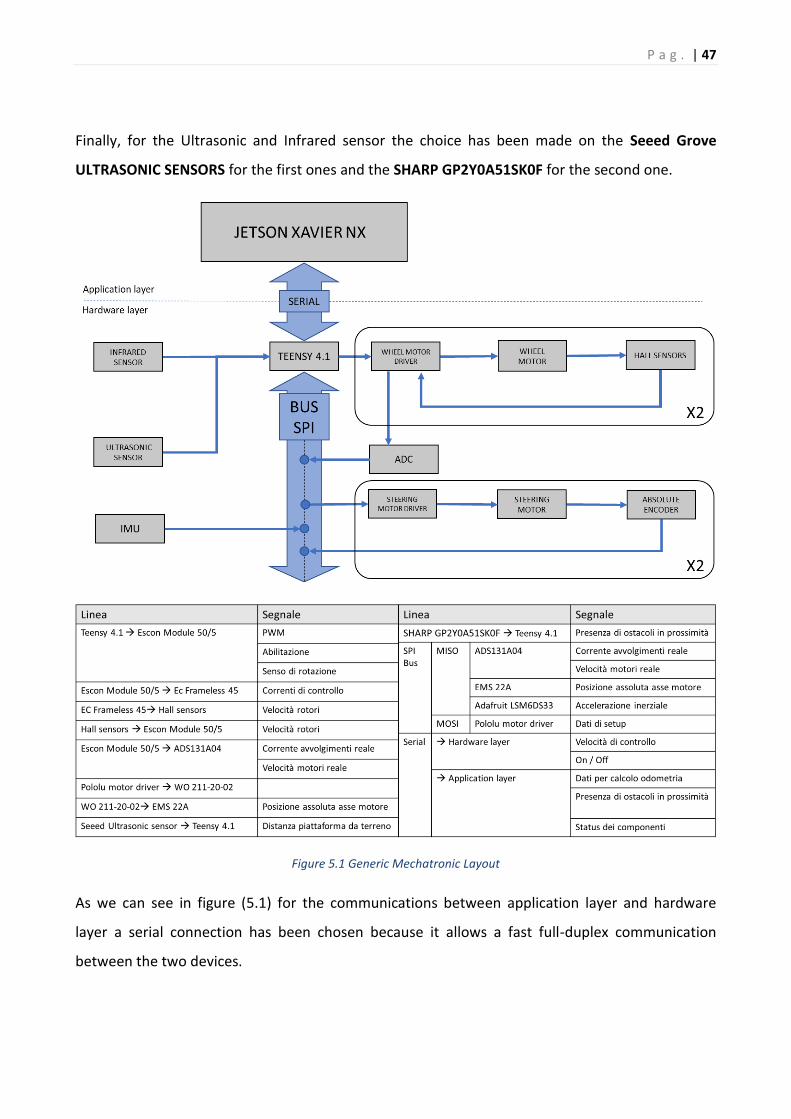
Finally, for the Ultrasonic and Infrared sensor the choice has been made on the Seeed Grove

ULTRASONIC SENSORS for the first ones and the SHARP GP2Y0A51SK0F for the second one.

Figure 5.1 Generic Mechatronic Layout

As we can see in figure (5.1) for the communications between application layer and hardware

layer a serial connection has been chosen because it allows a fast full-duplex communication

between the two devices.

P a g . | 48

The SPI Bus connect the IMU, the absolute encoder, the ADC and the stepper motor driver to the

microcontroller. The infrared and ultrasonic sensors don’t need to be putted on the bus because

they must warn the microcontroller whenever there is a proximity danger.

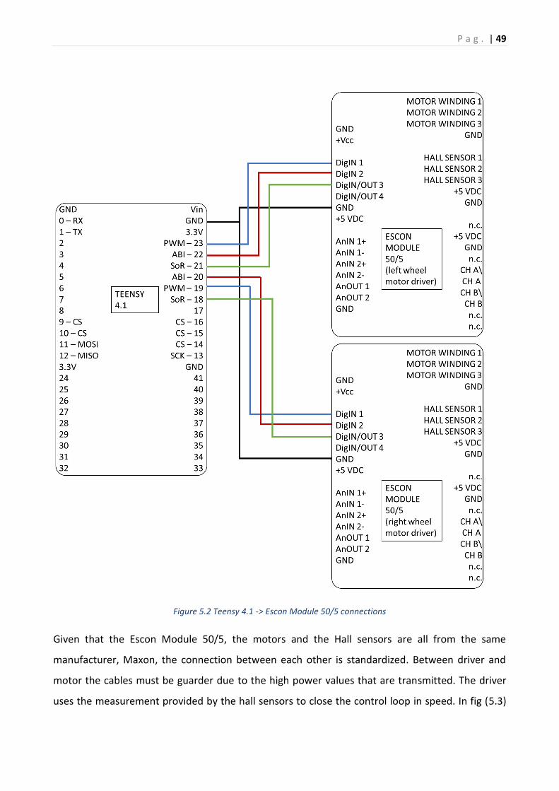
5.2 Wheel motor connections

The Escon Module 50/5 can be set up in various way. It has been decided to control the motor’s

speed via PWM generated by the Teensy 4.1. In addition, an enabling signal is used to allow the

motor motion and ii is a digital active high signal. Finally, the sense of rotation is determined by

another digital signal: when it is active high the motor will rotate counterclockwise and otherwise

it will rotate clockwise. In fig (5.2) the details of the connection between the Teensy 4.1 and the

Escon Module 50/5 can be seen.

P a g . | 49

Figure 5.2 Teensy 4.1 -> Escon Module 50/5 connections

Given that the Escon Module 50/5, the motors and the Hall sensors are all from the same

manufacturer, Maxon, the connection between each other is standardized. Between driver and

motor the cables must be guarder due to the high power values that are transmitted. The driver

uses the measurement provided by the hall sensors to close the control loop in speed. In fig (5.3)

P a g . | 50

the details of the connection between the Escon Module 50/5, the motors EC Frameless and the

Hall sensors can be seen.

Figure 5.3 Escon module 50/5 -> EC frameless 45 flat connections

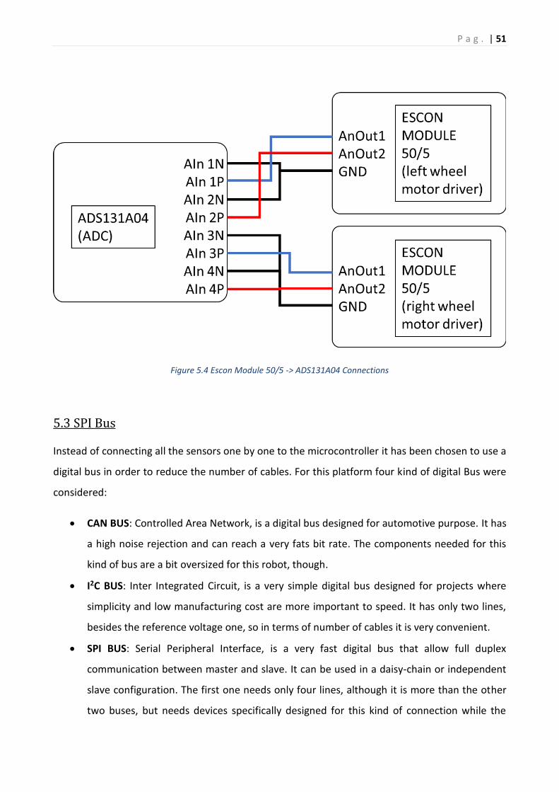
The Escon Module 50/5 allow to transmit important measurements through two analog output.

The chosen output are the real windings current and the real rotor speed. These two

measurements are used to compute the internal odometry of the platform. Because they are

analog signals an ADC is needed to convert them into digital signals. In fig (5.4) the details of the

connection between the Escon Module 50/5 and the ADC can be seen.

P a g . | 51

Figure 5.4 Escon Module 50/5 -> ADS131A04 Connections

5.3 SPI Bus

Instead of connecting all the sensors one by one to the microcontroller it has been chosen to use a

digital bus in order to reduce the number of cables. For this platform four kind of digital Bus were

considered:

• CAN BUS: Controlled Area Network, is a digital bus designed for automotive purpose. It has

a high noise rejection and can reach a very fats bit rate. The components needed for this

kind of bus are a bit oversized for this robot, though.

• I2C BUS: Inter Integrated Circuit, is a very simple digital bus designed for projects where

simplicity and low manufacturing cost are more important to speed. It has only two lines,

besides the reference voltage one, so in terms of number of cables it is very convenient.

• SPI BUS: Serial Peripheral Interface, is a very fast digital bus that allow full duplex

communication between master and slave. It can be used in a daisy-chain or independent

slave configuration. The first one needs only four lines, although it is more than the other

two buses, but needs devices specifically designed for this kind of connection while the

P a g . | 52

independent slave configuration is way faster but the master needs a pin dedicated for

every slave in addition to the other lines.

Although an I2C bus would be the best choice to have the smaller number of cables and

connections it has been chosen to use an SPI bus due to the need of this kind of bus to set-up the

Stepper drivers and so it was pointless to add another digital bus only for the sensors. The

preferrable configuration is the independent slave configuration because allow a higher

transmission speed and to configure the master-slave connection independently for each slave.

The SPI bus with independent slave configuration has three common lines plus a dedicated one for

every slave. Of the three common lines, one is dedicated to the clock, Serial Clock (SCK), and the

other two are for data transmission, one is defined Master-Output/Slave-Input (MOSI) and the

other one is defined Master-Input/Slave-Output (MISO). The SCK line is used to synchronize every

device to the master clock, while the on the other two take place the data transmission. Having

two lines dedicated to the data transmission allow a full-duplex communication, the master can

send data while receiving data. To select the device with which it wants to communicate, the

master uses the above-mentioned slave dedicated line, Chip Select (CS). When the master wants

to communicate with one slave it active the CS dedicated to that device and start “talking” while

the other devices are not activated. To prevent disturbance on the MISO line all the devices needs

a tristate logic connection: when not active this kind of connection assume a high-impedance

state, effectively removing the output from the circuit.

P a g . | 53

Figure 5.5 SPI Bus Connections

The master device is obviously the Teensy 4.1. The slave devices are the two stepper driver, the

two absolute encoder, the IMU and the ADC. The only two devices that receive data on the MOSI

line are the stepper drivers and they receive the set-up data as mentioned before. Instead the

MISO line is connected to every device on the bus:

• The two stepper drivers send eventual stall detection when microstepping

P a g . | 54

• The two absolute encoders send the absolute position of the steering shaft

• The IMU send the measured inertial accelerations and speeds

• The ADC send the converted real windings current and real rotor speed of the wheel

motors

In fig (5.5) we can see the details of the connection of the SPI bus.

5.4 Proximity Sensors connections

In the environment in which this robot will work not every obstacle can be determined a-priori. As

a matter of fact, every kind of unpredicted impediment can occur at every moment during the

motion. So, a set of proximity sensors is essential to avoid crash or fall during the motion. It isn’t

important to put this kind of sensor on the SPI bus because they are not meant to transmit data

regularly to the microcontroller, but only in case of imminent danger.

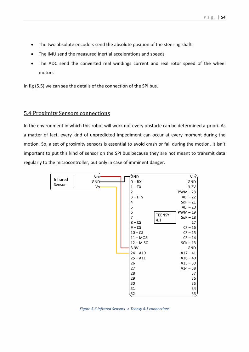
Figure 5.6 Infrared Sensors -> Teensy 4.1 connections

P a g . | 55

The presence of stairs inside the environment can put in danger of falling the robot. To avoid this

issue, infrared sensors are installed in proximity of each wheels to detect whenever the robot is

approaching a step. The voltage output of the chosen infrared sensors (SHARP GP2Y0A51SK0F) is

proportional to the distance measured in a range of 2-15 cm. In fig (5.6) we can see the details of

the connection of the infrared sensors.

To avoid crashes with unpredicted obstacle on the path such as a moved chair or a person,

ultrasonic sensors are installed all around the perimeter of the robot. The chosen sensors, GROVE

ultrasonic ranger, have a measuring range of 2-350 cm with an angle of 15 degree. The output is

PWM with the measured distance proportional to the impulse width. In fig (5.7) we can see the

details of the connection of the ultrasonic sensors.

Figure 5.7 Ultrasonic sensors -> Teensy 4.1 connections

P a g . | 56

5.5 Serial interface

The serial interface is between the hardware layer (HL) and the application layer (AL). It is

important to carefully determine what is transmitted between the serial interface because it will

condition the modularity of the robot. The serial port of the Teensy 4.1 are TTL level (transistor-

transistor logic) so to implement a RS-232 standard connection it is needed a MAX232 conversion

chip.

The HL needs to receive from the AL the data used to control the motion of the platform. Such

data is represented by the three components of the speed of the cassis that can be controlled in

the operative space as said in the section 3.2 of this thesis. These three components are:

• Longitudinal Speed: 𝑣𝑐,𝑥 = �̇�𝑐

• Transverse Speed: 𝑣𝑐,𝑦 = �̇�𝑐

• Yaw Speed: 𝜔𝑐,𝑧 = �̇�

The choice of this set of speed allow a clear separation between AL and HL. The AL will compute

the trajectory knowing only the degree of freedom of the platform without knowing the specific

control parameters of the platform used. As a matter of fact, it will be the HL to “translate” the set

of speed in the actual control speed for the actuator. Specifically for this platform it is important to

notice that all the different configurations are particular cases of the most general one and that

the configuration selection is implicit inside the set of speed chosen.

P a g . | 57

Figure 5.8 Communication Protocol Scheme

Recalling the description of the four configurations in section 3.7, it is important to notice how the

value of the speed select implicitly the configuration:

• Configuration I is the most general one, so this configuration is the one that the platform

uses whenever the other three are not used.

• Configuration II doesn’t allow the robot to translate but not to rotate, so whenever the

control yaw speed is equal to zero the configuration that the platform uses is this one.

• Configuration III, also known as Differential Drive, doesn’t allow values of speed along the

y-axis of {𝑐}, so whenever the control transverse speed is equal to zero the configuration

that the platform uses is the Differential Drive one.

• Configuration IV, also known as Bicycle, doesn’t allow values of speed along the x-axis of

{𝑐}, so, like before, whenever the control longitudinal speed is equal to zero the

configuration that the platform uses is the Bicycle one.

Summarizing the configuration is chosen from which of the control speed are equal to zero. If two

control speed are equal to zero, the robot is either translating along an axis or rotating on the

spot, so the chosen configuration is the bicycle one for translation along the y-axis, and the

differential drive for translation along the x-axis and for rotation on the spot.

P a g . | 58

It is important to recall that the bicycle configuration has important dynamic resistance from out-

of-the-plane solicitations. This dynamic characteristic is preserved for steering angle inside a small

neighbourhood of values centred on 𝛿𝑤𝑟 = 𝛿𝑤𝑙 =𝜋2⁄ . This little steering angle are part of the

configuration I and whenever they are used the platform will switch configuration automatically.

The risk is that if the AL doesn’t know to remain in these little neighbourhood at high speed, not

knowing the structure particularities, it can use a set of speed that impose bigger steering angle at

high speed causing a safety hazard. This issue can be overwhelmed by an initial instructing phase

where the AL “learn” how to control the platform.

On the other directions the AL needs primarily from the HL the necessary data to compute

odometry and, so the position if the robot. In order to maintain the modularity, the data sent from

the HL must be of the same kind of the control data, hence the AL must receive a set of speed

composed of:

• Measured Longitudinal Speed

• Measured Transverse Speed

• Measured Yaw speed

These threes speeds must be computed from the HL microcontroller starting from the data

collected from the sensors. In this way the separation between AL and HL is ensured and so they

can be designed separately and used with different modules.

Besides that, there are “survival” data that the AL needs to receive to properly control the robot.

These survival data are the warnings of the proximity sensors and the status of the HL

components. These kinds of data are not meant to be regularly sent over but only when they carry

on a warning. So whenever a proximity sensor detects an imminent danger or the microcontroller

detects a fault in some component the HL must transmit the information to the AL in order to stop

the robot and communicates the fault to the user.

P a g . | 59

Conclusion and Further Development

In this thesis the initial stages of the design of an assistive robot are analysed. The analysis is

focused on building strong basis on which develop a coherent design. As a matter of fact, all the

choice made about the design of this robot come out from a process that start at the very

beginning with the classification.

Defining those five classes of WMR with respect to their mobility is very helpful in understanding

the best structures in relation to the degree of mobility requested from the task of the robot. The

final choice concerning the components of the robot is made respecting the requirements came

out from the analysis of the various tasks that it must be able to perform. Approaching the design

in this way make the process a lot easier because every choice is a natural consequence of what

this robot is requested to do.

The final structure of this robot has two driven wheels and two castor wheels, to maximise

stability and mobility on the plane. In addition is introduced an important feature for this robot:

the modularity. This feature will allow a very high work field flexibility resulting in more appeal to

the buyer.

Once the mechanical structure is defined the kinetic analysis has been carried out to understand

fully the relation between the operative space and the joint space of this robot. It came out four

different operative configurations, each one with pros and cons that have been analysed as well,

in order to determine for every kind of motion which configuration is best at.

The way found to plan the trajectory of this robot is by using a Bézier polynomial with two control

points for the position and for the 𝛾 variable a straight line. In this way the tangent on the initial

and final point of the trajectory can be determined separately as the orientation on the plane can

be planned independently with respect to the position. It has been seen also how to implement a

law of motion with a geometric trajectory.

P a g . | 60

In the last chapter it is analysed the mechatronic layout in order to satisfy all the requirements,

especially for the modular feature. Using the kinematic analysis, a communication protocol that

allow a complete separation between high and low level is defined.

As a further development could be of interest developing various modules for various

environment of work. For example, the necessities of an office are different from the necessities

of a house. So, starting from the definition of the task needed by all the different work

environment it is interesting to develop various modules responding to those requirements.

P a g . | 61

References 1. United Nations, Department of Economic and Social Affairs. "World Population Ageing 1950-2050".

United Nations Publications. 2001.

2. Campion, G. "Structural Properties and Classification of Kinematic and Dynamic Models of Wheeled

Mobile Robots". IEEE Trans. Robot. Automat. 1996.

3. Han, K. L. "The source of Position Errors of Omni-directional Mobile Robot with Mecanum Wheel". IEEE.

2010.

4. Indiveri, G. "Swedish Wheeled Omnidirectional Mobile Robots: Kinematics Analysis and Control". IEEE

Trans. Robot. 2009.

5. F. G. Pin. "A New Family of Omnidirectional and Holonomic Wheeled Platforms for Mobile Robots". IEEE

Trans. Robot. Autom. 1994.

6. Jung, M. J. "Omni-directional Mobile Base OK-II". IEEE Intern. Confer. Robot. Automat. 2000.

7. Wada, M. "Holonomic and Omnidirectional Vehicle with Conventional Tires". IEEE Intern. Conf. Robot.

Automat. 1996.

8. Lauria, M. "Design and Control of a Four Steered Wheeled Mobile Robot". IEEE. 2006.

9. Hua, F. "Mechanical Design of a Four-wheel Independent Drive and Steering Mobile Robot Platform".

IEEE. 2016.

10. Gurol, B. "Mechanical and Electrical Design of a Four-Wheel-Drive, Four-Wheel-Steer Manipulator with

PA-10 Arm". IEEE. 2007.

11. Reiser, U. "Care-O-bot 3 - Creating a product vision for service robot applications by integrating design

and technology". IEEE/RSJ Intern. Conf. Intel. Robots Systems. 2009.

P a g . | 62

Ringraziamenti

Ringrazio in primo luogo la mia famiglia, che senza il loro perenne supporto non sarei mai riuscito

ad arrivare in fondo a questo percorso di studi.

Un enorme ringraziamento a Luca, colui che mi ha sostenuto e guidato in quest’ultimo periodo

nella stesura di questa Tesi, senza di lui sarei molto probabilmente ancora al titolo.

Un ringraziamento al Politecnico di Torino che mi ha fatto capire cosa significhi essere

un’eccellenza del panorama Universitario mondiale.

Un ringraziamento soprattutto ai miei amici di Torino e Pistoia, su cui ho potuto e potrò sempre

contare sia nel bisogno che nel divertimento.

Infine il ringraziamento più grande lo voglio riservare a Silvia, su cui non ho bisogno di spendere

altre parole perchè lei sa quanto sia stata fondamentale nel farmi arrivare a questo punto.