Political Aspects of Household Debt

Yun K. Kim, Gilberto Tadeu Lima, and Mark Setterfield __________________________WORKING PAPER 2017-02

________________________________

DEPARTMENT OF ECONOMICS

UNIVERSITY OF MASSACHUSETTS BOSTON ________________________________

Political Aspects of Household Debt∗

Yun K. Kim†, Gilberto Tadeu Lima‡, and Mark Setterfield§

August 17, 2017

Abstract

The recent literature has shown that income inequality is one of the main causesof borrowing and debt accumulation by working households. This paper explores thepossibility that household indebtedness is an important cause of rising income inequal-ity. If workers experience rising debt burdens, their cost of job loss may rise if theyneed labor-market income to continue borrowing and servicing existing debt. This,in turn, will reduce their bargaining power and increase income inequality, inducingworkers to borrow more in order to maintain consumption standards, and so creatinga vicious circle of rising inequality, job insecurity, and indebtedness. We believe thatthese dynamics may have contributed to observed simultaneous increases in income in-equality and household debt prior to the recent financial crisis. To explore the two-wayinteraction between inequality and debt, we develop an employment rent frameworkthat explicitly considers the impact of workers’ indebtedness on their perceived cost ofjob loss. This is embedded in a neo-Kaleckian macro model in which inequality spursdebt accumulation that contributes to household consumption spending and hence de-mand formation. Our analysis suggests that: (1) workers’ borrowing behavior plays acrucial role in understanding the character of demand and growth regimes; (2) debtand workers’ borrowing behavior play an important role in the labor market by influ-encing workers’ bargaining power; and (3) through such channels, workers’ borrowingbehavior can be a decisive factor in the determination of macroeconomic (in)stability.

Key words : Consumer debt, employment rent, cost of job loss, bargaining power, incomedistribution, growth, stability

JEL classifications : E12, E21, E24, E44, O41

∗Earlier versions of this paper were presented at the annual conference of the Eastern Economic Asso-ciation, New York, 2015, the 19th FMM Conference “The Spectre of Stagnation? Europe in the WorldEconomy,” Berlin, 2015, and seminars at Kingston University, the University of Greenwich, the University ofParis 13, Kyoto University, and Meji University. We would like to thank conference and seminar participantsand, in particular, Marc Lavoie, Antoine Godin, Peter Skott, Gary Dymski, Hiroaki Sassaki, and MichaelLaine for their helpful comments and suggestions. Any remaining errors are our own.†Department of Economics, University of Massachusetts Boston, Boston, MA; yun.kim@umb.edu.‡Department of Economics, University of Sao Paulo, Sao Paulo, Brazil; giltadeu@usp.br.§Department of Economics, New School For Social Research, New York, NY 10003;

mark.setterfield@newschool.edu.

1

1 Introduction

From the 1980s until the onset of the Great Recession, the US economy was characterized

by simultaneous increases in household indebtedness, income inequality, and consumption

expenditures. The income share of the top 1 percent of the income distribution rose from

approximately 8 percent in 1980 to almost 18 percent by 2007. Meanwhile, the ratio of

personal outlays to disposable personal income increased from about 88 percent in the early

1980s to nearly 100 percent in 2007. Finally, household debt as a share of GDP increased

from about 58 percent in 1975 to nearly 129 percent in 2007. A prominent argument in the

literature has been that these trends were closely linked. Specifically, rising income inequality

coupled with a desire on the part of households to maintain their relative standards of living

is thought to have been one of the main drivers of increased borrowing and debt accumulation

by less affluent (working) households (Palley, 2002; Barba and Pivetti, 2009; Kumhof et al.,

2015; Foster and Magdoff, 2009; Carr and Jayadev, 2015).

This paper explores a different dimension of the inequality/indebtedness nexus. In his

seminal article “Political Aspects of Full Employment”, Kalecki (1943) postulated that un-

employment plays an important role as a disciplinary device in a capitalist labor market.

We argue that household debt can play a similar role. This is because like unemployment

in Kalecki (1943), debt can act as a worker discipline device by raising the threat to their

well-being that workers associate with job loss. This, in turn, reduces workers’ willingness to

(inter alia) bargain for higher wages. Our argument is grounded in a number of recent ob-

servations to the effect that rising household indebtedness disempowers workers and affects

the wage bargain.1 According to Bonefeld (1995, p.69), debt undermines workers’ resistance

to wage reductions and the intensification of work, playing a critical role in “disciplining so-

cial relations to monetary scarcity and a life of hard and unrewarding labor to sustain basic

needs”. Similarly, Bryan et al. (2009, p.13) posit that “while the wage relation involves a

1These observations dovetail with more general empirical findings that “financialization” has been asource of increased income inequality (Kohler et al., 2015; Darcillon, 2016).

2

retrospective payment to labor for past surplus value, consumer credit as labor’s relation

with capital about the future, implies the rending of surplus value before participation in

“production” and so intensifies labor’s commitment to the production system itself”. Citing

Glyn (2006), meanwhile, Slater and Spencer (2014, p.142) argue that “financialization has

impacted directly on the employment relationship. Specifically, it has enabled employers to

increase their power over workers. As workers have accumulated financial assets and taken

on greater amounts of debt, they have become less able and willing to push for higher wages

and better working conditions ... Higher personal debt ratios increase the vulnerability of

those in work and the desperation of those without.” These claims are echoed in the findings

of, for example, Karacimen (2015), whose questionnaires and interviews with workers in the

Turkish metal working sector reveal that indebtedness transforms capital-labor relations,

ultimately increasing workers’ sense of commitment to their employers. In a similar fash-

ion Butrica and Karamcheva (2014) find that older adults with debt are 8 percentage points

more likely to work and 2 percentage points less likely to receive Social Security benefits than

those without debt, suggesting that, on balance, indebtedness compels older individuals to

keep working.

Building on Setterfield and Kim (2016) and Setterfield et al. (2016), in which rising

inequality in the presence of consumption emulation effects is linked to increasing indebted-

ness, we postulate that, simultaneously, debt is an important potential cause of rising income

inequality. Using an employment rent framework (Bowles, 1985, 2004; Schor and Bowles,

1987), we show how the rent workers associate with their current employment is affected by

their level of indebtedness. The possibility arises that as debt increases, so, too, does the cost

of job loss, reducing the willingness of workers to risk job loss in the process of negotiating

for higher wages. The diminution of workers’ power in the wage bargain thus causes slower

wage growth for working households, and so contributes to rising income inequality.2 This, in

2Note that, together with their ability to bargain (as reflected in, for example, the structure of laborlaw), we hereby treat the willingness of workers to bargain as one dimension of workers’ bargaining power.In what follows we refer to changes in the employment rent as affecting workers’ bargaining power on theunderstanding that it does so by affecting the willingness of workers to bargain, as described above.

3

turn, may induce additional borrowing by working households, so that what ultimately arises

is a two-way interaction between inequality and indebtedness in the form of a vicious circle.

We believe that this self-reinforcing cycle of inequality, indebtedness, and disempowerment

has contributed to the economic and political unsustainablity of the Neoliberal (1980–2007)

growth regime in the US economy. We show, however, that once we allow for bi-directional

causality in the relationship between household debt and income inequality, the relationship

between these variables (and its broader impact on a growing economy) is far from simple.

Much depends on workers’ borrowing behavior, and whether such behavior is principally

motivated by a target level of consumption or a target level of debt (and in either case,

to what extent). Ultimately, our analysis reveals that workers’ borrowing behavior plays a

decisive role in determining the stability properties of the economy.

Our paper is organized as follows. Sections 2 and 3 present the basic theoretical frame-

work, which gives rise to a stock-flow consistent Post-Keynesian growth model in which

inequality affects household indebtedness and vice-versa. Section 4 explores the dynamics

and macroeconomic consequences of this two-way interaction between debt accumulation

and income inequality. Finally, section 5 offers some concluding comments.

2 Accounting and Behavior in the Baseline Model

2.1 Social Accounting Matrices

We begin with a basic accounting framework that draws on Lavoie and Godley (2001-02) and

Godley and Lavoie (2007), and that distinguishes four types of agents: workers, capitalists,

banks, and non-financial firms. To focus our discussion, we assume a closed economy with

no government sector.

Table 1 is the balance sheet matrix for our model economy. It shows the asset and liability

allocations across the four types of agent. There are four classes of assets: physical capital

(K), equity (Q), net loans to working households and the corresponding net bank deposits

4

of capitalists (DW ).3 A column sum for a class of agent produces its net worth, while a row

sum (across workers, capitalists, banks, and firms) produces the net value of a class of assets.

Associated with this balance sheet matrix is the transaction flow matrix in table 2. House-

hold real wage income (WL), where W is the real wage and L is the level of employment,

can be supplemented by new borrowing (DW ) to finance the sum of workers’ consumption

(CW ) plus the interest accruing on their past borrowing (iDW , where the interest rate, i

is assumed fixed for simplicity).4 Capitalists earn income on their net deposits (iDW ) and

from profits (Π), which they use for consumption (CR), to make new deposits (DW ), or

to purchase equities (Q). In the case of firms, we distinguish between capital and current

transactions. Firms finance investment (I) with new funds provided by capitalists (Q) and

distribute all earnings to capitalists.5 For the transaction matrix, we note that the sums

across the rows must equal zero as a consistency condition.6 The columns also sum to zero,

reflecting agents’ budget constraints.

Table 1: Balance Sheet Matrix

Workers Capitalists Firms Banks Sum

Capital K KDeposits DW −DW 0Loans −DW DW 0Equities Q −Q 0Net worth NWW NWR NWF NWB K

3We assume throughout that DW > 0, thereby excluding the possibility that working households mightact as net creditors. This is consistent with the stylized facts of household balance sheets in recent decades(Barba and Pivetti, 2009; Carr and Jayadev, 2015).

4Note that implicit in this statement of workers’ budget constraint are the assumptions that workers donot save, and that workers’ debts are not amortized but instead roll over from period to period. In otherwords, debt servicing consists only of meeting interest payable on outstanding debt, so that as they continueto borrow, the total outstanding indebtedness of working households increases over time. Again, this isconsistent with the stylized facts of household balance sheets in recent decades (Barba and Pivetti, 2009;Carr and Jayadev, 2015).

5For simplicity, the price of equity is fixed and normalized to one.6This consistency condition reflects that one agent’s expenditure must be equal to another agent’s income

in the economy as a whole.

5

Table 2: Transaction Flow MatrixFirms Banks

Workers Capitalists Current Capital Current Capital Sum

Consumption −CW −CR CW + CR 0Investment I −I 0Wages WL −WL 0Firms’ profits Π −Π 0Deposit interest iDW −iDW 0Loan interest −iDW iDW 0

Change in deposit −DW DW 0

Change in loans DW −DW 0

Issues of equities −Q Q 0Sum 0 0 0 0 0 0 0

2.2 Banks and Firms

Our specification of the banking sector draws on Lavoie and Godley (2001-02) and Godley

and Lavoie (2007), similarly distinguishing the capital and current accounts. We refer to

financial intermediaries as “banks” and non-financial businesses as “firms”. Consumer loans

are intermediated by the banking sector. Banks are pure intermediaries that do not generate

profits. As such, we do not distinguish between the borrowing rate and the lending rate,

as (for instance) in Skott and Ryoo (2008a,b) and Isaac and Kim (2013). Capitalists hold

saving deposits with banks, on which they receive interest payments. Workers receive these

bank deposits as bank loans, with which they finance consumption expenditures.

Firms are characterized by their investment demand behavior and mark up pricing be-

havior. We treat the pricing behavior of firms in standard neo-Kaleckian fashion: price is

a mark up over unit labor costs, reflecting an oligopolistic market structure (Harris, 1974;

Asimakopulos, 1975; Dutt, 1984):

p = (1 + τ)wL/Y (1)

Here p is the price level, w is the nominal wage, τ is the mark up rate (which represents

Kalecki’s degree of monopoly), and L/Y is the labor-output ratio (i.e., the inverse of the

6

average product of labor). Such mark up pricing behavior implies a standard expression for

the gross profit share (π = Π/Y ):

π =τ

1 + τ(2)

Our exposition will treat τ and hence π as given in the short run. In the dynamics beyond the

short run, however, τ and hence π become endogenous variables as a result of distributional

conflict.

Let r = Π/K denote the profit rate. Firms’ desired investment rate (gK = I/K) responds

positively to the profit rate:

gK = κ0 + κrr (3)

The parameters of equation (3) are positive: κ0 captures the state of business confidence

or animal spirits (Keynes, 1936); and κr captures the sensitivity of desired investment to

the profit rate. The current profit rate approximates the expected rate of return, and hence

induces planned investment (Robinson, 1962; Blecker, 2002; Stockhammer, 1999).7

Since the profit rate can be expressed in terms of the capacity utilization rate (u = Y/K)

as:

r = πu (4)

it follows that the expression for the accumulation rate in equation (3) can be re-written as:

gK = κ0 + κrπu (5)

7Investment behavior is an important and contested subject in Post-Keynesian models. Since our focusis on workers’ borrowing and associated consumption behavior, we use a simple neo-Keynesian investmentfunction and leave extensions of our analysis that involve changing the form of the of the investment functionto future research.

7

2.3 Workers’ and Capitalists’ Households

Workers’ consumption behavior is given by:

CW = WL− iDW + DW (6)

The term WL− iDW denotes after-interest-payments disposable income, while DW captures

borrowing by workers. Equation (6) is consistent with workers’ budget constraint from

the first column of Table 2, which requires that DW = CW + iDW − WL. Normalizing

working households’ consumption by the capital stock, and noting that dW = DWK⇒ dW =

DWK− gKdW ⇒ DW

K= dW + gKdW , we can re-write (6) as:

cW = (1− π)u− idW + dW + gKdW (7)

Workers’ debt-financed consumption behavior plays a pivotal role in the analysis to follow.

We use the following behavioral function to describe this behavior:

dW = f(dW , ψ) (8)

where ψ = 1 − π denotes the wage share of income. Equation (8) suggests that workers’

borrowing depends on their previously accumulated debt and their wage income. Note that

equation (8) specifies workers’ normalized borrowing behavior,8 rather than their absolute

level of borrowing (DW ) in any period. Since dW = DWK⇒ dW = DW

K− gKdW as pre-

viously noted, it follows that the level of workers’ borrowing DW = [dW + gKdW ]K is an

endogenous residual in our model, determined by equation (8) in conjunction with the rate

of accumulation, gK .

There are various combinations of economically reasonable behavior that might sign the

partial derivatives of the function in equation (8), and so describe the precise manner in

8Normalized, as are the other variables in our model, by the capital stock.

8

which working households approach the process of debt accumulation. Hence if workers are

mindful of the need to generate sufficient wage income to service outstanding debts, their

borrowing may increase in the wage share (fψ > 0); however, workers might alternatively

reduce borrowing as they receive higher wages (fψ < 0), if their borrowing is motivated

principally by an exogenous target level of consumption (more of which can now be funded

by current income). Workers’ borrowing may increase in the level of indebtedness (fdW > 0),

meanwhile, since more debt increases the debt-servicing burden and hence the need to borrow

to achieve an exogenous target level of consumption. On the other hand, working households

might behave more frugally, reducing their borrowing in response to an increase in their

indebtedness (fdW < 0) if they are mindful of exceeding an exogenous target debt level. As

this brief discussion reveals, the description of borrowing behavior in (8) ultimately allows

for partial derivatives of differing signs depending on whether workers’ borrowing behavior

is principally driven by consumption considerations (such as an exogenous target level of

consumption) or financial considerations (such as an exogenous target level of debt) (see,

for example, Setterfield and Kim (2016) and Dutt (2005, 2006), respectively). Note also

that the larger the magnitude of the partial derivatives of equation (8), the quicker will

be the adjustment of workers’ borrowing (and consumption) behavior to changes in their

indebtedness and the wage share. As will become clear, the magnitudes (as well as the signs)

of the partial derivatives of (8) play an important role in the economy’s macrodynamics.

Capitalists’ consumption, meanwhile, is a fixed proportion of their total (profit plus

interest) income:

CR = (1− sR)(Π + iDW ) (9)

where sR is capitalists’ saving coefficient.9 Normalizing capitalists’ consumption equation

9Equivalently, capitalists’ saving is given by SR = sR(Π + iDW ). Recalling capitalists’ budget constraintfrom the second column of table 2, equilibrium in the consumer credit market therefore requires that:

DW = sR(Π + iDW )− Q (10)

Note that this equality holds in equilibrium, when saving by capitalist households fully funds autonomousspending by workers as well as investment by firms. It does not imply that our model is subject to a

9

by the capital stock, we get:

cR = (1− sR)(π + idW ) (11)

2.4 Temporary Equilibrium

Commodity market equilibrium in our model has a standard representation:

Y = CW + CR + I (12)

Normalizing (12) by the capital stock and substituting equations (5), (7), (8), and (11) into

the resulting expression, we arrive at:

u = ψu+ f(dW , ψ) + gKdW + (1− sR)(1− ψ)u− sRidW + κ0 + κr(1− ψ)u (13)

Solving for u yields the following reduced-form expression for capacity utilization:

u =κ0 + (κ0 − sRi)dW + f(dW , ψ)

(sR − κr − κrdW )(1− ψ)(14)

Substituting (14) into (4) and (5), meanwhile, yields accompanying reduced-form expressions

for the rates of profit and accumulation:

r =κ0 + (κ0 − sRi)dW + f(dW , ψ)

(sR − κr − κrdW )(15)

gK =κ0sR − κrsRidW + κrf(dW , ψ)

(sR − κr − κrdW )(16)

Clearly, the temporary equilibrium values of u, r, and gK depend on both the wage share

and the (normalized) indebtedness of working households. Workers’ borrowing behavior

therefore plays a crucial role in determining the relationship between effective demand and

savings-in-advance constraint, which would prevent it from being demand-led. In other words, some form ofendogenous credit creation is required in order for the model to traverse from one steady state configurationto another. Since our interest is purely in the characteristics of the steady state itself, however, we abstractfrom this monetary feature of disequilibrium adjustment for the sake of simplicity.

10

income distribution. Hence note that:

∂u

∂ψ=κ0 + (κ0 − sR)idW + f(dW , ψ) + (1− ψ)fψ

(sR − κr − κrdW )(1− ψ)2(17)

The standard “Keynesian stability condition” implies that (sR − κr − κrdW ) > 0. It follows

that if workers borrow more to finance consumption as wages rise (fψ > 0), the likelihood

that ∂u∂ψ

> 0 (i.e., demand is wage-led) increases. However, if workers reduce their debt-

financed consumption as wages rise (fψ < 0) and do so aggressively, the derivative in (17)

could become negative, resulting in a profit-led demand regime.10

Workers’ borrowing behavior also dictates the relationship between the profit and ac-

cumulation rates and income distribution, determining whether (and the extent to which)

growth is profit-led or wage-led. Hence:

∂r

∂ψ=

fψsR − κr − κrdW

(18)

∂gK∂ψ

=κrfψ

sR − κr − κrdW(19)

If workers borrow more aggressively to maintain their consumption standards in the event

of rising income inequality (fψ < 0), the rates of profit and growth will increase and we will

observe profit-led growth. If, however, workers borrow more only when they feel they can

afford to take on more debt by virtue of having higher wages (fψ > 0), the derivatives in

(18) and (19) turn positive resulting in wage-led growth.11

Workers’ borrowing behavior also plays an important role in determining the relationships

between effective demand, profit, and growth rates on one hand, and the indebtedness of

10Note that the size of the wage share itself will also influence this possibility, and hence whether thedemand regime is wage- or profit-led.

11Note that our results here are in line with previous studies that examine the implications of debt-financedconsumption for wage-led vs. profit-led demand and growth regimes (Setterfield and Kim, 2017).

11

working households on the other. Hence:

∂u

∂dW=

(κ0 + i(κr − sR))sR + κrf(dW , ψ) + (sR − κr − κrdW )fdW(sR − κr − κrdW )2(1− ψ)

(20)

∂r

∂dW=

(κ0 + i(κr − sR))sR + κrf(dW , ψ) + (sR − κr − κrdW )fdW(sR − κr − κrdW )2

(21)

∂gK∂dW

=(κr(κ0 + i(κr − sR))sR + κrf(dW , ψ) + (sR − κr − κrdW )fdW )

(sR − κr − κrdW )2(22)

If workers borrow more aggressively to maintain consumption when their indebtedness and

hence the debt-servicing claims on their wage income increase (fdW > 0), the derivatives in

(20) – (22) will be positive.12 The economy will exhibit debt-led demand and growth regimes.

However, if working households respond more frugally to their indebtedness (fdW < 0) and

reduce their debt-financed consumption aggressively, the derivatives in (20) – (22) may turn

negative and the economy will then exhibit debt-burdened demand and growth regimes.13

3 Extending the Model: Household Debt and the Cost

of Job Loss

So far, we have considered only how the distribution of income affects household indebted-

ness. We now turn to the question of how household indebtedness affects income distribution.

Our starting point is the employment rent framework of Bowles (1985, 2004) and Schor and

Bowles (1987). This we write as:

E = W −(hWu +

[1− h

]W ′)

(23)

12This is assured if κ0 > i(κr − sR)sR, which is a reasonable condition since 0 < i, sR < 1.13Note that the size of workers’ debt burdens will also influence this possibility, and hence whether the

demand and growth regimes are debt-led or debt-burdened.

12

where W is, as defined earlier, the real wage that a worker receives in their current employ-

ment, h is the probability that a displaced worker will be unemployed if he/she loses his/her

current job, Wu is the income that a worker receives while unemployed (e.g., unemployment

insurance benefits), and W ′ is the real wage that a worker will receive if they are re-employed

upon loss of their current employment, where W ≥ W ′ > Wu. We assume, for the sake of

simplicity, that workers use current period values as an indication of expected future states

and that h is exogenously given. Although h is the perceived probability of unemployment

(rather than re-employment) in the event of job loss, we assume that no actual job loss takes

place among currently employed workers. Instead, the probability of unemployment h is a

credible threat to the status of currently employed workers as currently employed workers.

We do not allow for actual transitions of currently employed workers into a state of unem-

ployment so as to abstract from questions related to the capacity of formerly unemployed

workers to continue servicing debts accrued while they were employed. As a result, any

variations in the quantity of employment implied by local adjustments towards the steady

state in the course of our stability analysis in section 4 are assumed to be achieved through

variation in the hours worked by an otherwise fixed number of persons employed.14

In light of the aggregate level at which our model is developed, we need to redefine the

employment rent in (23) so that it represents the value of remaining in employment to all

currently employed workers. Multiplying by the level of employment, L, and noting that we

also have W ′ = W (since ours is a one sector growth model with homogeneous labor), the

14This is consistent with our treatment of h as exogenously given (and hence independent of local adjust-ments in u towards its steady state value). To see this, suppose we think of h as being proxied by the currentrate of unemployment U , so that:

h = U = 1− L

N= 1− L

Y

Y

K

K

N= 1− auk (24)

where N is the labor force, a is the ratio of the total number of persons employed to total output, and k isthe ratio of the capital stock to the labor force (not to be confused with the capital-labor ratio associatedwith the production technology on the supply side). Since by definition k = k(gK−n), where n is the rate ofgrowth of the labor force, we can treat k as constant (k = 0) by postulating that n = gK – that is, the rateof growth of the labor force adjusts endogenously to meet the needs of a growing capitalist economy throughinter-sectoral and/or inter-regional migration of a global “reserve army” of labor. With k thus fixed, anylocal variation in u implied by our stability analysis is absorbed in our model by local variation in a, leavingh unchanged.

13

employment rent expression in (23) becomes:

EL = WL−(hWuL+

[1− h

]WL

)(25)

Now consider how the value of this aggregate employment rent EL is modified by the

fact that workers borrow to finance some part of their consumption spending and (as a

consequence) carry debt that must be serviced from current income. We assume that workers

can only borrow in this fashion if they are currently employed: in other words, jobs effectively

act as collateral for loans. In this case, borrowing privileges are part of the benefit of

employment, whereas loss of borrowing privileges is part of the cost of being unemployed.15

In light of these considerations, the value of EL can be re-written as:

EL = WL+ DW − iDW −(h

[WuL− iDW

]+

[1− h

][WL+ DW − iDW

])(26)

which represents the aggregate employment rent with household debt. Note that DW = 0 in

the event of unemployment, consistent with the assumption that having jobs act as collateral

for loans. If we now assume for simplicity that Wu = 0,16 the expression in (26) simplifies

to:

EL = h[WL+ DW ] (27)

Normalizing by the capital stock and once again recalling that DW/K = dW + gKdW =

15Recall that, as previously explained, local variations in u are assumed to be absorbed by local variationsin hours worked (rather than the unemployment rate). It is, then, strictly the binary distinction betweenhaving or not having a job (rather than variation in hours worked by those employed) that affects thecapacity to borrow and hence the value of the employment rent in our analysis. In fact, variation in hoursworked, and the tightness or slack in the labor market that this might appear to imply, has no effect on thevalue of the employment rent in our model.

16Recall that the transition from employment to unemployment is a credible threat not a physical statein this model. Hence setting the income associated with unemployment to zero does not mean that ourdebt dynamics are affected by default as a result of previously employed workers becoming unemployed (andearning no income), since no such transitions of state (from employment to unemployment) actually occur.

14

f(dW , ψ) + gKdW using equation (8), we obtain the normalized aggregate employment rent

with household debt :

e = h[ψu+ f(dW , ψ) + gKdW ] (28)

The expression in (28) is a measure of indebted workers’ collective bargaining power. When

there is an increase in e, so that the perceived cost of joss is higher, workers attach more

value to retaining their current positions of employment. Consequently, they will be less

willing to engage in behaviors that may result in job loss – such as bargaining for higher

wages.

Bearing in mind the temporary equilibrium rates of capacity utilization and growth in (14)

and (16), the expression for e in (28) sets up a complicated relationship between indebtedness,

income distribution, and workers’ aggregate employment rent. Hence:

∂e

∂dW= h[ψ

∂u

∂dW+ fdW +

∂gK∂dW

dW + gK ] (29)

Note that if workers borrow more aggressively when they are more indebted (fdW > 0), we

see ∂u∂dW

, ∂gK∂dW

> 0 in equations (20) and (22). This will insure that an increase in workers

indebtedness will increase the cost of job loss ( ∂e∂dW

> 0). In this scenario, an increase

in indebtedness induces more borrowing in order to debt-finance consumption spending.

Because jobs are required for borrowing, this increases the value of employment to workers

and hence the employment rent, resulting in a reduction of workers’ bargaining power.

However, if workers are frugal, and reduce their borrowing as they become more indebted

(fdW < 0), we may observe the opposite result. An increase in indebtedness increases debt

servicing commitments which, by reducing after-interest-payments disposable income, has a

negative effect on consumption. This reduces the value to workers of their jobs and lowers the

employment rent. An increase in indebtedness, meanwhile, induces less borrowing to finance

consumption, which also makes jobs less valuable and lowers the employment rent. And if

workers reduce their debt-financed consumption aggressively, we may see ∂u∂dW

, ∂gK∂dW

< 0 as

15

discussed at the end of section 2.4. In this case, an increase in workers’ indebtedness will

decrease the cost of job loss, resulting in an increase in workers’ bargaining power.

Similarly, with regard to income distribution:

∂e

∂ψ= h[ψ + ψ

∂u

∂ψ+ fψ +

∂gK∂ψ

dW ] (30)

If workers borrow more aggressively when they receive a higher real wage (fψ > 0), we

see ∂u∂ψ, ∂gK∂ψ

> 0 in equations (17) and (19). This will insure that an increase in the wage

share will increase the cost of job loss ( ∂e∂ψ

> 0). Intuitively, an increase in the real wage

induces more borrowing to finance consumption. Both the increase in the real wage itself

and the increase in borrowing, which is only possible when workers are employed, makes

employment more valuable and so increases the employment rent. This will have a negative

effect on workers’ bargaining power.

However, if workers borrow less as they receive a higher wage (fψ < 0), the effect of a

wage increase on e is ambiguous. A decrease in borrowing brought about by a wage increase

makes employment less valuable, since borrowing to finance consumption is part of the value

of a job. However, a real wage increase has a directly positive effect on the employment rent,

since in and of itself a higher real wage makes a job more valuable. We therefore observe

two opposing effects arising from the same increase in wages. If workers’ seek to reduce

their debt financed consumption aggressively, we may observe ∂u∂ψ, ∂gK∂ψ

< 0 as can be seen in

equations (17) and (19). This will result in a decrease in the cost of job loss, raising workers’

bargaining power. The notion that an increase in the real wage can reduce the employment

rent (and so increase workers’ bargaining power) is counterintuitive, since ceteris paribus a

higher real wage undoubtedly makes jobs more valuable. But as the discussion above reveals,

once we entertain the possibility of debt-financed consumption spending by workers, other

things may not be equal. Indeed, with fψ < 0 and |fψ| large, and with part of the value of a

job deriving from the fact that jobs act as collateral for loans, it is possible that, on balance,

16

an increase in the real wage will decrease the value of holding a job and so reduce the size

of the employment rent.

4 Dynamics

In this section, debt and distribution dynamics arising form the model outlined in the two

previous sections are described. We then analyze the interaction of these dynamics and their

implications for the steady state configurations of our model. We treat dW and ψ as state

variables. Equation (8) – repeated below for ease of reference – is thus relevant for our

analysis in this section:

dW = f(dW , ψ)

As previously discussed, the signs of the partial derivatives of (8) will differ depending on

the precise borrowing behavior of workers.

We begin describing our distribution dynamics by writing:

ψ = ϕ(e) , ϕe < 0 (31)

Equation (31) is based on the logic of the employment rent: the higher is e, the less inclined

are workers to engage in activity – such as bargaining for higher real wages and hence a

higher wage share – that could be construed as conflictual and that could therefore result

subsequently in job loss. Now recall from equation (28) that:

e = h(ψu+ f(dW , ψ) + gKdW )

Combining this expression with (31) and recalling equations (14) and (16) (which show that

both u and gK are functions of ψ and dW ), we can write:

ψ = ϕ(h[ψu+ f(dW , ψ) + gKdW ]) = φ(dW , ψ) (32)

17

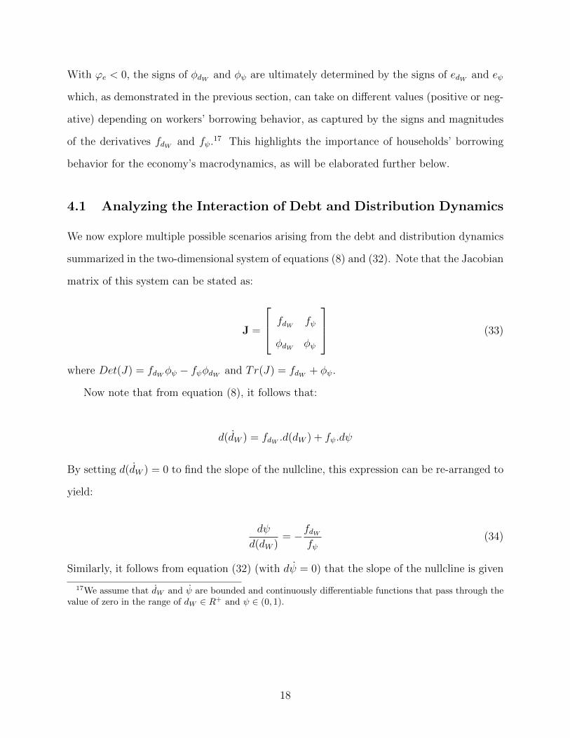
With ϕe < 0, the signs of φdW and φψ are ultimately determined by the signs of edW and eψ

which, as demonstrated in the previous section, can take on different values (positive or neg-

ative) depending on workers’ borrowing behavior, as captured by the signs and magnitudes

of the derivatives fdW and fψ.17 This highlights the importance of households’ borrowing

behavior for the economy’s macrodynamics, as will be elaborated further below.

4.1 Analyzing the Interaction of Debt and Distribution Dynamics

We now explore multiple possible scenarios arising from the debt and distribution dynamics

summarized in the two-dimensional system of equations (8) and (32). Note that the Jacobian

matrix of this system can be stated as:

J =

fdW fψ

φdW φψ

(33)

where Det(J) = fdWφψ − fψφdW and Tr(J) = fdW + φψ.

Now note that from equation (8), it follows that:

d(dW ) = fdW .d(dW ) + fψ.dψ

By setting d(dW ) = 0 to find the slope of the nullcline, this expression can be re-arranged to

yield:

dψ

d(dW )= −fdW

fψ(34)

Similarly, it follows from equation (32) (with dψ = 0) that the slope of the nullcline is given

17We assume that dW and ψ are bounded and continuously differentiable functions that pass through thevalue of zero in the range of dW ∈ R+ and ψ ∈ (0, 1).

18

as:

dψ

d(dW )= −φdW

φψ(35)

Understanding the dynamics of the system becomes a question of determining the relative

slopes of the nullclines, which is dictated by the partial derivatives that appear on the right

hand sides of equations (34) and (35), bearing in mind the expressions for the determinant

and trace of the Jacobian matrix in equation (33). As there could be different dynamic

configurations around the steady state, three different cases are discussed here as behaviorally

plausible examples of the dynamics that might arise form our model.

4.1.1 Case 1

First, recall that we can state that fψ > 0 ⇒ eψ > 0, and hence φψ < 0. If borrowing

is increasing in the wage share (fψ > 0), because households are mindful of the need to

generate sufficient wage income to service debt, the rate of change of the wage share is

decreasing in the wage share (φψ < 0), because a higher wage share raises the value of the

employment rent (eψ > 0) and so reduces the bargaining power of workers. Now recall

also that fdW > 0 ⇒ edW > 0, and hence φdW < 0. Borrowing increases in the level

of indebtedness (fdW > 0) because more debt and hence more debt servicing creates the

need to borrow more to finance consumption. Because a job is required for borrowing, this

increases the value of employment and hence the value of the employment rent (edW > 0).

This will reduce workers’ bargaining power and hence φdW < 0. We therefore have:

dψ

d(dW )

∣∣∣dW=0

= −fdWfψ

< 0

dψ

d(dW )

∣∣∣ψ=0

= −φdWφψ

< 0

In this case, one possibility that arises is that:

19

dψ

d(dW )

∣∣∣dW=0

>dψ

d(dW )

∣∣∣ψ=0

⇒ −fdWfψ

> −φdWφψ

⇒ fdWφψ − fψφdW > 0 (36)

This situation is depicted in Figure 1. The inequality in (36) indicates that D(J) > 0 in

(33). Moreover, since fdW > 0 and φψ < 0, we will have Tr(J) < 0 in (33) as long as workers’

positive borrowing response to their increased indebtedness is relatively weak (fdW > 0 is

small – the relatively frugal case). In this case, the debt dynamics nullcline is flat relative to

the wage share nullcline – as in Figure 1 – and the dynamic system summarized by equations

(8) and (32) will be stable.

ψ

dW

ψ*

dW*

Figure 1: Stable Dynamics for Case 1

20

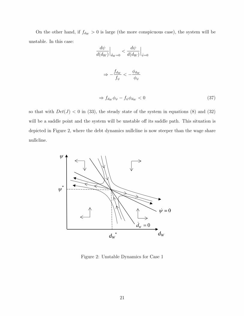
On the other hand, if fdW > 0 is large (the more conspicuous case), the system will be

unstable. In this case:

dψ

d(dW )

∣∣∣dW=0

<dψ

d(dW )

∣∣∣ψ=0

⇒ −fdWfψ

< −φdWφψ

⇒ fdWφψ − fψφdW < 0 (37)

so that with Det(J) < 0 in (33), the steady state of the system in equations (8) and (32)

will be a saddle point and the system will be unstable off its saddle path. This situation is

depicted in Figure 2, where the debt dynamics nullcline is now steeper than the wage share

nullcline.

ψ

dW

ψ*

dW*

Figure 2: Unstable Dynamics for Case 1

21

4.1.2 Case 2

Next, consider the case in which, together with fψ > 0 and φψ < 0 as in case 1, worker

households are so frugal as to aggressively reduce their debt-financed consumption whenever

there is an increase in their indebtedness. In other words, fdW < 0 and |fdW | is large. As

discussed in section 3, this will result in edW < 0 and hence φdW > 0. Intuitively, the

decreased proclivity to borrow reduces the value of jobs (which are required in order to

borrow and debt-finance consumption). And if this effect is sufficiently strong, it generates

a reduction in the employment rent and so increases workers’ bargaining power, with the

final result that φdW > 0. We now have two positively sloped nullclines:

dψ

d(dW )

∣∣∣dW=0

= −fdWfψ

> 0

dψ

d(dW )

∣∣∣ψ=0

= −φdWφψ

> 0

In this case, we have:

Tr(J) = fdW + φψ < 0

There are two possibilities for Det(J), meanwhile. The first creates a stable system. When

the debt dynamics nullcline has a steeper slope than the wage share dynamics nullcline

because |fdW | is large, so that −fdWfψ

> −φdWφψ

, we observe:

Det(J) = fdWφψ − fψφdW > 0

However, it is also possible for the system to be only saddle-path stable as long as |fdW |

is not too large, so that −fdWfψ

< −φdWφψ

and hence:

Det(J) = fdWφψ − fψφdW < 0

22

Once again, we see that the magnitude (not just the sign) of workers’ bargaining and bor-

rowing responses to changes in indebtedness and the wage share has an important effect on

the economy’s macrodynamics. It is also worth noting that for any given |fdW |, the size of

|φdW | can become decisive in determining macro stability. In other words, the size of the

indirect effect of fdW , working via the employment rent and hence the marginal effect of debt

on the wage share, also exerts an important influence eon the economy’s macrodynamics.

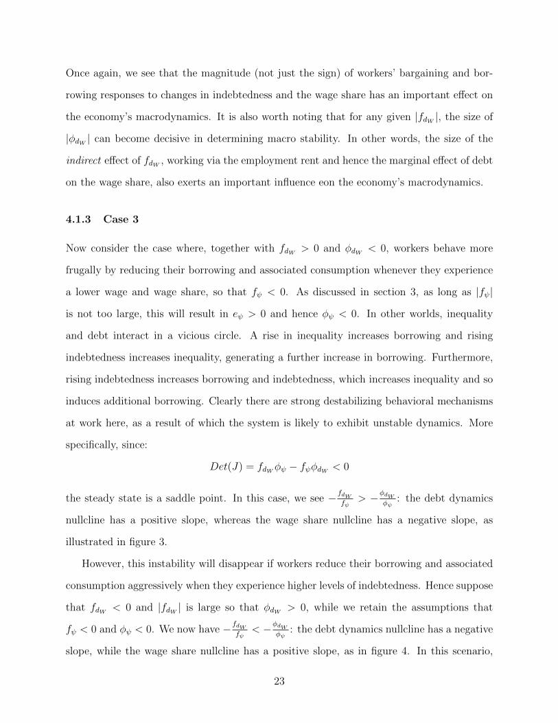
4.1.3 Case 3

Now consider the case where, together with fdW > 0 and φdW < 0, workers behave more

frugally by reducing their borrowing and associated consumption whenever they experience

a lower wage and wage share, so that fψ < 0. As discussed in section 3, as long as |fψ|

is not too large, this will result in eψ > 0 and hence φψ < 0. In other worlds, inequality

and debt interact in a vicious circle. A rise in inequality increases borrowing and rising

indebtedness increases inequality, generating a further increase in borrowing. Furthermore,

rising indebtedness increases borrowing and indebtedness, which increases inequality and so

induces additional borrowing. Clearly there are strong destabilizing behavioral mechanisms

at work here, as a result of which the system is likely to exhibit unstable dynamics. More

specifically, since:

Det(J) = fdWφψ − fψφdW < 0

the steady state is a saddle point. In this case, we see −fdWfψ

> −φdWφψ

: the debt dynamics

nullcline has a positive slope, whereas the wage share nullcline has a negative slope, as

illustrated in figure 3.

However, this instability will disappear if workers reduce their borrowing and associated

consumption aggressively when they experience higher levels of indebtedness. Hence suppose

that fdW < 0 and |fdW | is large so that φdW > 0, while we retain the assumptions that

fψ < 0 and φψ < 0. We now have −fdWfψ

< −φdWφψ

: the debt dynamics nullcline has a negative

slope, while the wage share nullcline has a positive slope, as in figure 4. In this scenario,

23

ψ

dW

ψ*

dW*

Figure 3: Unstable Dynamics for Case 3

rising inequality increases borrowing. But rising indebtedness reduces the employment rent,

empowers workers, and ultimately reduces inequality. Furthermore, rising indebtedness will

now reduce borrowing directly. We now observe strong stabilizing behavioral mechanisms,

which inevitably gives rise to stable system dynamics since:

Det(J) = fdWφψ − fψφdW > 0

and:

Tr(J) = fdW + φψ < 0

4.1.4 Summary

The various cases considered above are not exhaustive. Nevertheless, what is clearly estab-

lished by and important to take away from the preceding discussion is that workers’ borrow-

ing behavior plays a decisive role in determining whether or not the economy is stable when

there is a two-way interaction between household indebtedness and income inequality, such

24

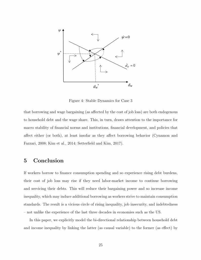
ψ

dW

ψ*

dW*

Figure 4: Stable Dynamics for Case 3

that borrowing and wage bargaining (as affected by the cost of job loss) are both endogenous

to household debt and the wage share. This, in turn, draws attention to the importance for

macro stability of financial norms and institutions, financial development, and policies that

affect either (or both), at least insofar as they affect borrowing behavior (Cynamon and

Fazzari, 2008; Kim et al., 2014; Setterfield and Kim, 2017).

5 Conclusion

If workers borrow to finance consumption spending and so experience rising debt burdens,

their cost of job loss may rise if they need labor-market income to continue borrowing

and servicing their debts. This will reduce their bargaining power and so increase income

inequality, which may induce additional borrowing as workers strive to maintain consumption

standards. The result is a vicious circle of rising inequality, job insecurity, and indebtedness

– not unlike the experience of the last three decades in economies such as the US.

In this paper, we explicitly model the bi-directional relationship between household debt

and income inequality by linking the latter (as causal variable) to the former (as effect) by

25

means of the Bowles-Schor employment rent framework. We have shown that the vicious

circle interaction between indebtedness and inequality outlined above is possible, but that

in fact the debt-inequality relationship is far from straightforward: the two-way interaction

between these variables can have a variety of consequences for the macrodynamics of a grow-

ing economy. We are nevertheless able to establish three clear results that have important

theoretical and policy implications. First, workers’ borrowing and associated debt-financed

consumption behavior plays an important role in determining the responsiveness of effective

demand and growth to exogenous variations in income distribution, thus influencing the ba-

sic wage- or profit-led as well as debt-burdened or debt-led characters of effective demand

and growth regimes. Second, household debt and workers’ borrowing behavior play an im-

portant role in the labor market, affecting the cost of job loss and hence workers’ bargaining

power, and so exerting a second influence on macroeconomic dynamics via the (now endoge-

nous) distribution of income. Finally, workers’ borrowing behavior plays a crucial role in

determining macroeconomic stability.

Our results are in keeping with the claims of Skott (2017, pp.343-53) that beyond a first

approximation the distribution of income should not be treated as exogenous, and that labor

market (as well as goods market) considerations must be factored into analyses of growth and

distribution. They also lend further credence to the notion, increasingly common in Post-

Keynesian macrodynamics, that for all the attention that has previously been paid to firms

and their behavior (and in particular, the form of the investment function), the household

sector now merits at least as much attention: with the widespread availability of consumer

credit, consumption and household borrowing behavior may be at least as important as

investment and corporate borrowing behavior for determining the basic characteristics of

demand and growth regimes, and macroeconomic stability.

26

References

Asimakopulos, Athanasios (1975, August). “A Kaleckian theory of income distribution.”

Canadian Journal of Economics 8(3), 313–333.

Barba, Aldo and Massimo Pivetti (2009). “Rising household debt: Its causes and macroe-

conomic implications—a long-period analysis.” Cambridge Journal of Economics 33(1),

113–137.

Blecker, Robert (2002). “Distribution, demand, and growth in neo-Kaleckian macro models.”

In Mark Setterfield, ed., The Economics of Demand-Led Growth: Challenging the Supply-

Side Vision of the Long Run, pp. 129–152. Cheltenham: Edward Elgar.

Bonefeld, W. (1995). “The politics of debt: social discipline and control.” Common Sense:

Journal of the Conference of Socialist Economists 17, 69–91.

Bowles, Samuel (1985). “The production process in a competitive economy: Walrasian,

Neo-Hobbesian, and Marxian models.” American Economic Review 75(1), 16–36.

Bowles, S. (2004). Microeconomics: Behavior, Institutions and Evolution. Princeton, NJ,:

Princeton University Press.

Bryan, Dick, Randy Martin, and Mike Rafferty (2009). “Financialization and Marx: Giving

labor and capital a financial makeover.” Review of Radical Political Economics 41(4),

458–472.

Butrica, Barbara A. and Nadia S. Karamcheva (2014). “Does household debt influence

the labor supply and benefit claiming decisions of older Americans?” Technical report,

Netspar Discussion Paper No. 03/2014-083, http://dx.doi.org/10.2139/ssrn.2574724.

Carr, Michael D. and Arjun Jayadev (2015). “Relative income and indebtedness: Evidence

from panel data.” Review of Income and Wealth 61(4), 759–772.

27

Cynamon, Barry Z. and Steven M. Fazzari (2008). “Household debt in the consumer age:

Source of growth—risk of collapse.” Capitalism and Society 3(2), Article 3.

Darcillon, Thibault (2016). “Do interactions between finance and labour market institutions

affect the income distribution?” Universite Paris1 Pantheon-Sorbonne Working Paper

hal-01248984, HAL.

Dutt, Amitava K. (1984). “Stagnation, income distribution and monopoly power.” Cam-

bridge Journal of Economics 8(1), 25–40.

Dutt, Amitava K. (2005). “Consumption, debt and growth.” In Mark Setterfield, ed.,

Interactions in Analytical Political Economy, pp. 155–78. Armonk, NY: M.E. Sharpe.

Dutt, Amitava K. (2006). “Maturity, stagnation and consumer debt: a Steindlian approach.”

Metroeconomica 57, 339–364.

Foster, John Bellamy and Fred Magdoff (2009). The Great Financial Crisis. New York, New

York: Monthly Review Press.

Glyn, T.L.A. (2006). Capitalism Unleashed : Finance, Globalization, and Welfare: Finance,

Globalization, and Welfare. Oxford: Oxford University Press.

Godley, W. and M. Lavoie (2007). Monetary Economics: An Integrated Approach to Credit,

Money, Income, Production and Wealth. London: Palgrave Macmillan.

Harris, Donald J. (1974). “The price policy of firms, the level of employment and distribution

of income in the short run.” Australian Economic Papers 13, 144–151.

Isaac, Alan G. and Yun K. Kim (2013). “Consumer and corporate debt: A neo-Kaleckian

synthesis.” Metroeconomica 64(2), 244–271.

Kalecki, M. (1943). “Political aspects of full employment.” The Political Quarterly 14(4),

322–330.

28

Karacimen, Elif (2015). “Interlinkages between credit, debt and the labour market: evidence

from Turkey.” Cambridge Journal of Economics 39(3), 751–767.

Keynes, John Maynard (1936). The General Theory of Employment, Interest and Money.

London: Macmillan.

Kohler, Karsten, Alexander Guschanski, and Engelbert Stockhammer (2015). “How does

financialisation affect functional income distribution? a theoretical clarification and em-

pirical assessment.” Economics Discussion Papers 2015-5, School of Economics, Kingston

University.

Kim, Yun K, Mark Setterfield, and Yuan Mei (2014). “A theory of aggregate consumption.”

European Journal of Economics and Economic Policies: Intervention 11(1), 31–49.

Kumhof, Michael, Romain Ranciere, and Pablo Winant (2015). “Inequality, leverage and

crises.” American Economic Review 105(3), 1217–1245.

Lavoie, Marc and Wynne Godley (2001-02). “Kaleckian models of growth in a coherent

stock-flow monetary framework.” Journal of Post Keynesian Economics 24(2), 277–311.

Palley, Thomas I. (2002). “Economic contradictions coming home to roost? does the US

economy face a long-term aggregate demand generation problem?” Journal of Post Key-

nesian Economics 25, 9–32.

Robinson, Joan (1962). Essays in the theory of economic growth. New York, New York: St

Martin’s press.

Schor, Juliet B. and Samuel Bowles (1987). “Employment rents and the incidence of strikes.”

The Review of Economics and Statistics 69(4), 584–92.

Setterfield, Mark and Yun K. Kim (2016). “Debt servicing, aggregate consumption, and

growth.” Structural Change and Economic Dynamics 36, 22–33.

29

Setterfield, Mark and Yun K. Kim (2017). “Household borrowing and the possibility of

consumption-driven, profit-led growth.” Review of Keynesian Economics 5(1), 43–60.

Setterfield, Mark, Yun K. Kim, and Jeremy Rees (2016). “Inequality, debt servicing, and

the sustainability of steady state growth.” Review of Political Economy 28(1), 45–63.

Skott, Peter (2017). “Weaknesses of ’wage-led growth’.” Review of Keynesian Eco-

nomics 5(3), 336 – 359.

Skott, Peter and Soon Ryoo (2008a). “Financialization in kaleckian economies with and

without labor constraints.” Intervention: European Journal of Economics and Economic

Policies 5(2), 357–386.

Skott, Peter and Soon Ryoo (2008b). “Macroeconomic implications of financialisation.”

Cambridge Journal of Economics 32(6), 827–862.

Slater, Gary and David A. Spencer (2014). “Workplace relations, unemployment and finance-

dominated capitalism.” Review of Keynesian Economics 2(2), 134 – 146.

Stockhammer, Engelbert (1999). “Robinsonian and Kaleckian growth. an update on Post-

Keynesian growth theories.” Working Paper 67, Vienna University of Economics and

Business Administration.

30