pollutants controlled calculation and...
TRANSCRIPT

Pollutants ControlledCalculation and Documentation
forSection 319 Watersheds
Training Manual
Revised June 1999
Michigan Department of Environmental QualitySurface Water Quality Division
Nonpoint Source UnitP.O. Box 30273
Lansing, Michigan 48909http:\\www.deq.state.mi.us
John Engler, GovernorRussell J. Harding, Director
2
CONTENTS
PAGEINDEX OF FIGURES............................................................................................................................3
INTRODUCTION...................................................................................................................................4
LEARNING OBJECTIVES ...................................................................................................................5
SEDIMENT REDUCTIONI. Background: Erosion and Sediment Delivery .......................................................................6
II. Gully Stabilization: ................................................................................................................. 10
III. Streambank/Ditchbank and Roadbank Stabilization; Livestock Exclusion ...................... 15
IV. Agricultural Fields................................................................................................................... 23
V. Filter Strips.............................................................................................................................. 34
FEEDLOT POLLUTION REDUCTION ............................................................................................. 38
INTEGRATED CROP MANAGEMENT REPORTING FOR PESTICIDES, COMMERCIALFERTILIZER, and MANURE UTILIZATION ..................................................................................... 44
GLOSSARY ..................................................................................................................................... 48
TECHNICAL REFERENCES ............................................................................................................. 50
EXHIBITS COVER PAGE .................................................................................................................. 51
Exhibit 1. Dry Density Soil Weights .......................................................................................... 52Exhibit 2. Soil Texture Triangle and Correction Factors for Soil Texture.............................. 53Exhibit 3. Feedlot Pollution Reduction Worksheet.................................................................. 54Exhibit 4. Integrated Crop Management Quarterly Summary Report ................................... 59
The Michigan Department of Environmental Quality (MDEQ) will not discriminate against any individual or group on thebasis of race, sex, religion, age, national origin, color, marital status, disability, or political beliefs. Questions or concernsshould be directed to the Office of Personnel Services, P.O. Box 30473, Lansing, Michigan 48909.
Printed by Authorit y of 1994 P.A. 451
Total number of copies 100 Total Cost:$ 230.00 Cost per copy: $ 2.30
Michi gan Department of Environmental Quality

3
INDEX OF FIGURES
PAGE
Figure 1. Lateral Recession Rates of Stream/Ditchbanks as Estimated by Field Observation 16
Figure 2. Lateral Recession Rates of Roadbanks as Estimated by Field Observations ........... 17
Figure 3. Contributing Area Examples ............................................................................................ 23
Figure 4. Sediment Delivery Ratio Based on Contributing Drainage Area.................................. 25
Figure 5. Phosphorus and Nitrogen Content of Sediment Delivered by Sheet and RillErosion ..................................................................................................................................... 26
Figure 6. Sample Feedlot ................................................................................................................. 39
Figure 7. 25-Year, 24-Hour Rainfall for Michigan........................................................................... 40
Figure 8. Curve Numbers for Feedlots............................................................................................ 39
Figure 9. Ratio of Chemical Oxygen Demand (COD) and Total Phosphorus (P) Produced byVarious Animals to That Produced by a 1,000 Pound Slaughter Steer........................................ 41
Figure 10. First Quarter ICM Report ................................................................................................ 46
Figure 11. Second Quarter ICM Report .......................................................................................... 47
Exhibit 1. Dry Density Soil Weights ................................................................................................. 52
Exhibit 2. Soil Texture Triangle and Correction Factors for Soil Texture .................................... 53
Exhibit 3. Feedlot Pollution Reduction Worksheet......................................................................... 54
Exhibit 4. Integrated Crop Management Quarterly Summary Report .......................................... 59

4
INTRODUCTION
This document provides instruction to the watershed technician regarding calculating anddocumenting pollutant reduction for the Surface Water Quality Division’s Nonpoint SourceProgram. It can also be used in other watershed projects that treat the sources of sedimentand nutrient pollutants using similar systems of Best Management Practices (BMPs). Thepurpose is to standardize the progress reporting in order that water quality impacts andstatewide achievements can be systematically represented.
It is recognized that this system has limitations, but it does provide a uniform system ofestimating relative pollutant loads. The methods are simple in concept and workable within afield office. This document includes instructions and examples regarding the calculation anddocumentation of pollutant reductions for: 1) sediment; 2) sediment-borne phosphorus andnitrogen; 3) feedlot runoff; and 4) commercial fertilizer, pesticides and manure utilization.
Water quality impacts from wind erosion will not be estimated. The dynamics of wind erosionand resulting atmospheric deposition do not perform similar to water erosion and quantifyingthese relationships for water quality is currently not possible. Likewise, the impacts of BMPson ground water quality are not well enough understood to make pollutant reduction estimatesfeasible.
The following people contributed to this document: Ruth Shaffer, Gary Rinkenberger and SeanDuffey, USDA-NRCS; and John Suppnick and Thad Cleary, Michigan Department ofEnvironmental Quality, Surface Water Quality Division.
Questions should be directed to the Michigan Department of Environmental Quality, NonpointSource Unit. The telephone number is 517-335-2867.

5
LEARNING OBJECTIVES
At the end of this training manual, the participant will be able to:
1. Define the term “Best Management Practices” (BMPs) and give examples used to treatdifferent kinds of erosion;
2. Define erosion and sediment delivery and explain the difference between theseprocesses;
3. List the assumptions that are used to relate gross erosion to resulting water qualityimpacts;
4. Calculate sediment and sediment-borne nutrient reductions from installation ofconservation practices to control gully erosion;
5. Define Lateral Recession Rate and explain how it is determined in the field;
6. Calculate sediment and sediment-borne nutrient reductions from streambank/ditchbanktreatment, livestock exclusion and from roadbank treatment.
7. Define Sediment Delivery Ratio, Nutrient Enrichment, Contributing Area, and how theserelate to estimation of sediment delivery from upland agricultural fields.
8. Calculate sediment and sediment-borne nutrient reductions from implementation ofconservation practices to control sheet and rill erosion from riparian fields.
9. Calculate additional savings in sediment and nutrients from the establishment of riparianfilter strips.
10. Accurately complete the required reporting form for Integrated Crop Management withNonpoint Source Program quarterly reports.

6
SEDIMENT REDUCTION
I. Backgr ound: Erosion and Sediment Delivery
The implementation of systems of Best Management Practices (BMPs) reduces nonpointsource pollution. BMPs are defined as structural, vegetative, or managerial conservationpractices, which reduce or prevent detachment, transport and delivery of nonpoint sourcepollutants to surface or ground waters. The BMPs result in less soil being transported anddeposited as sediment as well as fewer nutrients being delivered to the water bodies.
The BMPs in a water quality project must be targeted to priority fields within the watershed.Priority fields are cropland, pastureland or hayland that contribute runoff to adjacent hydrologicsystems such as lakes, streams, ditches, wetlands and flood plains. Reporting of pollutantreductions will be done for all priority fields where BMPs have been installed.
Sediment and nutrient reduction is estimated by first calculating gross erosion at a site, thencalculating the amount of soil and nutrients that are transported to the surface waters.Sediment and sediment-borne nutrients originate from various types of erosion. Each of theseerosion types can be estimated by accepted methods of technology to determine grosserosion. The Revised Universal Soil Loss Equation (RUSLE), the Gully Erosion Equation(GEE), and the Channel Erosion Equation will be used to calculate gross erosion. The varioustypes of erosion and the equations used to calculate gross erosion are discussed later in thischapter.
It is important to recognize the difference between “soil loss” as measured by these erosionequations and the sediment delivery to water bodies. Erosion is a naturally occurring process,which is defined as the wearing away or disintegration of earth material by the physical forcesof moving water and wind. Sediment delivery is the amount or fraction of soil that is actuallydelivered to a water body.
To relate gross soil erosion to water quality impacts, certain assumptions and professionaljudgments need to be made. Sediment delivery and the nutrient content of the sediment willbe estimated using other equations and values from the scientific literature.
Finally, it is important to know how soil loss tolerance relates to water quality. Soil losstolerance, as measured by equations such as the Revised Universal Soil Loss Equation, is ameasure of the amount of soil that can be removed from a site before soil productivity onsite isaffected. It is a soil quality term, not water quality. It is not a measure of the amount of soilthat moves offsite. Other factors such as proximity to a water body and the size of the areacontributing sediment to the edge of the field must be considered to determine the amount ofsediment that actually reaches water.
The following assumptions will be made when calculating sediment and nutrient reductions:
1. The point of deposition at the edge of field will be the basis for the sediment and nutrientreduction estimates. Sediment can be deposited into a stream, lake, ditch, or a wetland orfloodplain adjacent to a stream, lake or ditch. All of these water bodies are important andwarrant pollutant protection. Therefore, it will be our intent to represent the sediment andnutrient reduction at the boundary where the agricultural field or site joins these hydrologicsystems. The amount of sediment delivered to the edge of the field may be 100% in thecase of streambank or gully erosion sites directly on or adjacent to a water body. In thecase of upland erosion sites, the percent of soil delivered to the water as sediment will be

7
less than 100%; we will discuss how to estimate the amount delivered to a water body fromupland erosion sites later in this chapter.
2. Once the system of BMPs is established, the stabilized condition is assumed to control allthe erosion. Therefore the “before” condition is measured in average annual tons ofsediment generated (i.e., without treatment), and the “after” condition is assumed to benegligible.
3. Phosphorus and nitrogen reductions are assumed to come from reduction in sediment-borne nutrients. Nutrients that are dissolved and carried by runoff waters are not included.
4. Pollutant reduction savings are reported to the nearest whole number (i.e., 8 instead of8.23).

8
Student Exercise 1.
1. Define “erosion” and “sediment delivery”.
2. True or False: The soil loss tolerance is a measure of the amount of soil that is deposited ina water body.
3. The basis for calculating sediment and nutrient reduction estimates will be the point of__________________________________.

9
Student Exercise 1. - Answers
1. Define “erosion” and “sediment delivery”.
Erosion is the wearing away or disintegration of earth material by the physical forces ofmoving wind and water.
Sediment delivery is the amount or fraction of soil that is actually delivered to a water body.
2. True or False: The soil loss tolerance is a measure of the amount of soil that is deposited ina water body.
False. Soil loss tolerance is a measure of the amount of soil that can be removed from a sitebefore soil productivity is affected onsite.
3. The basis for calculating sediment and nutrient reduction estimates will be the point ofdeposition at the edge of the field.

10
II. Gully Stabilization
The Gully Erosion Equation (GEE) will be used for calculating annual sediment and attachedphosphorus and nitrogen reductions. These calculations are based on the NRCS Field OfficeTechnical Guide, Section I-C, Gully Erosion Equation:
Sediment Reduction:
Gully Erosion Equation (GEE) =
Top Width(ft.) + Bottom Width(ft.)/2 x Depth(ft.) x Length(ft) x Soil Weight (tons/ft 3)Number of Years
Refer to Exhibit 1 in the Appendix for dry density soil weights for different soil textures. Thenumber of years that a gully took to form (listed in the equation’s denominator) can beestimated from field records, from discussions with the landowner, or from observation andprofessional judgment.
The GEE can be used to estimate sediment and nutrient reduction following the installation ofthe following conservation practices:
1. Grade Stabilization Structure2. Grassed Waterway3. Critical Area Planting in areas with gullies4. Water and Sediment Control Basin
Once the conservation practice is established, the stabilized condition will have controlled allthe gully erosion. Therefore, report the average annual tons of gross erosion as sedimentdelivered at the edge of the field (100% delivery).
Report conservation practices separately. For example, if a grade stabilization structure andgrassed waterway are installed together at one site, the GEE should be used to estimate thesediment reduction from each practice and they should be reported separately.
Nutrient Reduction:
Nutrient reduced (lb/yr) =
Sediment reduced (T/yr) x Nutrient conc. (lb/lb soil) x 2000 lb/T x correction factor
The amount of attached phosphorus and nitrogen is calculated using information collected byUSDA-ARS researchers (Frere et al., 1980). The estimate starts with an overall phosphorusconcentration of 0.0005 lbP/lb of soil and a nitrogen concentration 0.001 lbN/lb of soil. Then ageneral soil texture is determined, and a correction factor is used to better estimate nutrient-holding capacity (Exhibit 2 in Appendix). A loamy soil has a correction factor of 1.0, while clayand muck soils are greater than 1.0 and sandy soils are less than 1.0. This correction factorreflects the fact that soils with higher clay and organic matter contents have a higher capacityto hold nutrients, while sandier soils have a lower nutrient capacity.

11
The following example illustrates how to calculate sediment and nutrient reductions.
Example 1 .
Farmer Brown installs an aluminum toewall set back 20 feet from the stream, and 480 linearfeet of grassed waterway. The soil texture is a loamy sand. The gully can be divided intothree reaches A, B and C. Reach A is 8 feet wide at the top, 4 feet deep, 3 feet wide at thebottom and 200 linear feet long. Reach B is 5 feet wide at the top, 2 feet deep, 2 feet wide atthe bottom and 150 linear feet. Reach C is 3 feet wide at the top, 1 foot deep, 1 foot wide atthe bottom and 130 linear feet. The gully was formed in three years. Calculate the sedimentand nutrient reductions for each practice.
Sediment Reduction Calculations:
Grade Stabilization Structure:
Sediment = (8ft. + 3ft)/2 x 4ft x 20ft x 0.055 tons/ft3 = 8 tons/yr.3 years
Grassed Waterway:Reach A:
Sediment = (8ft + 3ft)/2 x 4ft x 200ft x 0.055 tons/ft3 = 80.7 tons/yr.3 years
Reach B:
Sediment = (5ft + 2ft)/2 x 2ft x 150ft x 0.055 tons/ft3 = 19.3 tons/yr.3 years
Reach C:
Sediment = (3ft + 1ft)/2 x 1ft x 130ft x 0.055 tons/ft3 = 4.8 tons/yr.3 years
Total sediment reduction (grassed waterway) = A + B + C = 104.8 tons/yr.Round to 105 tons/yr.
Nutrient Reduction Calculation :
Nutrient reduced (lb/yr) =
Sediment reduced (T/yr) x Nutrient conc. (lb/lb soil) x 2000 lb/T x correction factor
The phosphorus reduction is calculated by multiplying the phosphorus concentration by thesediment reduction and correcting for the soil texture. The same method is used to calculatethe nitrogen reduction. Use a soil phosphorus concentration of 0.0005 lbP/lb soil, and a soilnitrogen concentration of 0.001 lbN/lb soil (Frere et al., 1980). According to Exhibit 2, a loamysand is classified as a Sand and has a correction factor of 0.85:
12
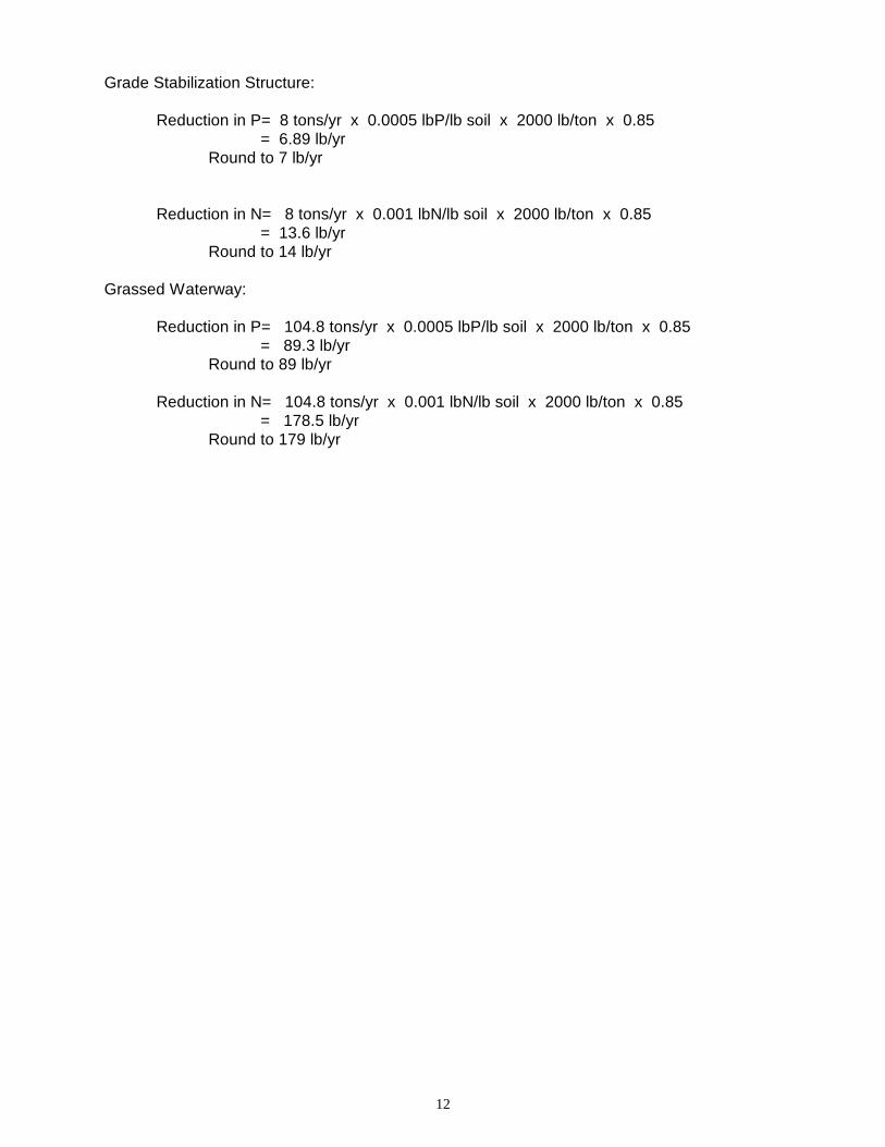
Grade Stabilization Structure:
Reduction in P= 8 tons/yr x 0.0005 lbP/lb soil x 2000 lb/ton x 0.85= 6.89 lb/yr
Round to 7 lb/yr
Reduction in N= 8 tons/yr x 0.001 lbN/lb soil x 2000 lb/ton x 0.85= 13.6 lb/yr
Round to 14 lb/yr
Grassed Waterway:
Reduction in P= 104.8 tons/yr x 0.0005 lbP/lb soil x 2000 lb/ton x 0.85= 89.3 lb/yr
Round to 89 lb/yr
Reduction in N= 104.8 tons/yr x 0.001 lbN/lb soil x 2000 lb/ton x 0.85= 178.5 lb/yr
Round to 179 lb/yr

13
Student Exercise 2.
1. A geotextile chute and a critical area planting are installed on a gully that is 10 feet from acounty drain. The soil texture is a silty clay loam. The original gully was 3 feet wide at thetop, 3 feet deep, 2 feet wide at the bottom and 15 linear feet long. The gully was formed inthree years. Calculate the sediment and nutrient reductions for each practice.
2. Explain why the soil phosphorus rate of 0.0005 lbP/lb of soil is modified with a correctionfactor for soil texture.

14
Student Exercise 2. - Answers
1. A geotextile chute and a critical area planting are installed on a gully that is 10 feet from acounty drain. The soil texture is a silty clay loam. The original gully was 3 feet wide at thetop, 3 feet deep, 2 feet wide at the bottom and 15 linear feet long. The gully was formed inthree years. Calculate the sediment and nutrient reductions for each practice.
Geotextile Chute Sediment and Nutrient Reduction:
Sediment reduced = (3ft + 2ft)/2 x 3ft x 10ft x 0.04 tons/ft3 = 1 ton/yr3 yrs
Reduction in P = 1 ton/yr x 0.0005 lbP/lb soil x 2000 lb/ton x 1.0= 1 lb/yr
Reduction in N = 1 ton/yr x 0.001 lbN/lb soil x 2000 lb/ton x 1.0= 2 lbs/yr
Critical Area Planting Sediment and Nutrient Reduction:
Sediment reduced = (3ft + 2ft)/2 x 3ft x 15ft x 0.04 tons/ft3 = 1.5 tons/yr3 yrs
Round to 2 tons/yr
Reduction in P = 1.5 tons/yr x 0.0005 lbP/lb soil x 2000 lb/ton x 1.0= 1.5 lbs/yr
Round to 2 lbs/yr
Reduction in N = 1.5 tons/yr x 0.001 lbN/lb soil x 2000 lb/ton x 1.0= 3 lbs/yr
2. Explain why the soil phosphorus rate of 0.0005 lbP/lb of soil is modified with a correctionfactor for soil texture.
The correction factor reflects the fact that soils with higher clay and organic matter contentshave a higher capacity to hold phosphorus, while sandier soils have a lower phosphorus-holding capacity.
15
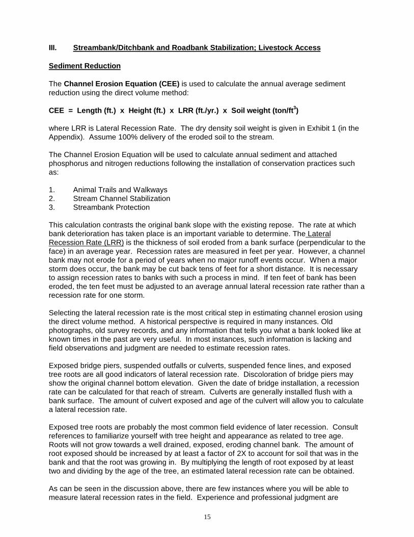
III. Streambank/Ditchbank and Roadbank Stabilization; Livestock A ccess
Sediment Reduction
The Channel Erosion Equation (CEE) is used to calculate the annual average sedimentreduction using the direct volume method:
CEE = Length (ft.) x Height (ft.) x LRR (ft./yr.) x Soil weight (ton/ft 3)
where LRR is Lateral Recession Rate. The dry density soil weight is given in Exhibit 1 (in theAppendix). Assume 100% delivery of the eroded soil to the stream.
The Channel Erosion Equation will be used to calculate annual sediment and attachedphosphorus and nitrogen reductions following the installation of conservation practices suchas:
1. Animal Trails and Walkways2. Stream Channel Stabilization3. Streambank Protection
This calculation contrasts the original bank slope with the existing repose. The rate at whichbank deterioration has taken place is an important variable to determine. The LateralRecession Rate (LRR) is the thickness of soil eroded from a bank surface (perpendicular to theface) in an average year. Recession rates are measured in feet per year. However, a channelbank may not erode for a period of years when no major runoff events occur. When a majorstorm does occur, the bank may be cut back tens of feet for a short distance. It is necessaryto assign recession rates to banks with such a process in mind. If ten feet of bank has beeneroded, the ten feet must be adjusted to an average annual lateral recession rate rather than arecession rate for one storm.
Selecting the lateral recession rate is the most critical step in estimating channel erosion usingthe direct volume method. A historical perspective is required in many instances. Oldphotographs, old survey records, and any information that tells you what a bank looked like atknown times in the past are very useful. In most instances, such information is lacking andfield observations and judgment are needed to estimate recession rates.
Exposed bridge piers, suspended outfalls or culverts, suspended fence lines, and exposedtree roots are all good indicators of lateral recession rate. Discoloration of bridge piers mayshow the original channel bottom elevation. Given the date of bridge installation, a recessionrate can be calculated for that reach of stream. Culverts are generally installed flush with abank surface. The amount of culvert exposed and age of the culvert will allow you to calculatea lateral recession rate.
Exposed tree roots are probably the most common field evidence of later recession. Consultreferences to familiarize yourself with tree height and appearance as related to tree age.Roots will not grow towards a well drained, exposed, eroding channel bank. The amount ofroot exposed should be increased by at least a factor of 2X to account for soil that was in thebank and that the root was growing in. By multiplying the length of root exposed by at leasttwo and dividing by the age of the tree, an estimated lateral recession rate can be obtained.
As can be seen in the discussion above, there are few instances where you will be able tomeasure lateral recession rates in the field. Experience and professional judgment are
16
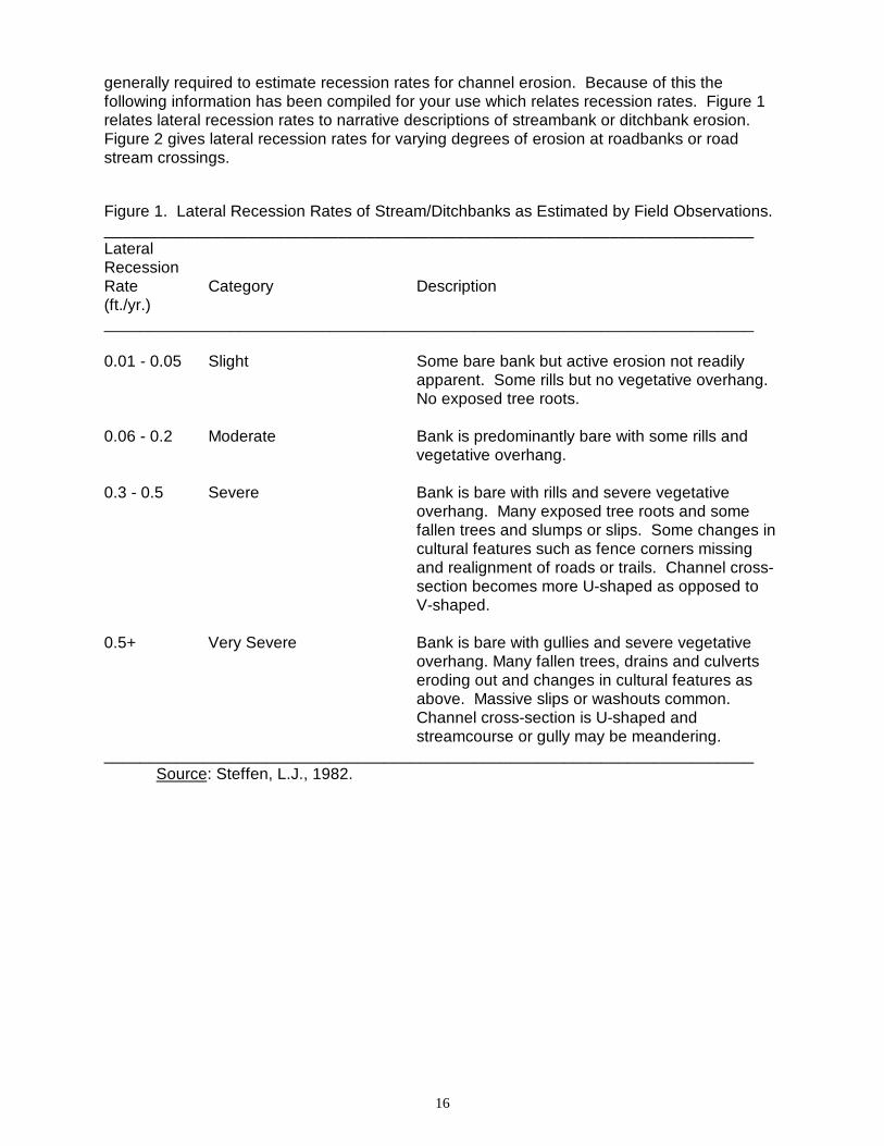
generally required to estimate recession rates for channel erosion. Because of this thefollowing information has been compiled for your use which relates recession rates. Figure 1relates lateral recession rates to narrative descriptions of streambank or ditchbank erosion.Figure 2 gives lateral recession rates for varying degrees of erosion at roadbanks or roadstream crossings.
Figure 1. Lateral Recession Rates of Stream/Ditchbanks as Estimated by Field Observations.________________________________________________________________________LateralRecessionRate Category Description(ft./yr.)________________________________________________________________________
0.01 - 0.05 Slight Some bare bank but active erosion not readilyapparent. Some rills but no vegetative overhang.No exposed tree roots.
0.06 - 0.2 Moderate Bank is predominantly bare with some rills andvegetative overhang.
0.3 - 0.5 Severe Bank is bare with rills and severe vegetativeoverhang. Many exposed tree roots and somefallen trees and slumps or slips. Some changes incultural features such as fence corners missingand realignment of roads or trails. Channel cross-section becomes more U-shaped as opposed toV-shaped.
0.5+ Very Severe Bank is bare with gullies and severe vegetativeoverhang. Many fallen trees, drains and culvertseroding out and changes in cultural features asabove. Massive slips or washouts common.Channel cross-section is U-shaped andstreamcourse or gully may be meandering.
________________________________________________________________________Source: Steffen, L.J., 1982.

17
Figure 2. Lateral Recession Rates of Roadbanks as Estimated by Field Observations.________________________________________________________________________LateralRecessionRate Category Description(ft./yr.)________________________________________________________________________
0.01 - 0.05 Slight Some bare roadbank but active erosion not readilyapparent. Some rills but no vegetative overhang.Ditch bottom is grass or noneroding.
0.06 - 0.15 Moderate Roadbank is bare with obvious rills and somevegetative overhang. Minor erosion orsedimentation in ditch bottom.
0.16 - 0.3 Severe Roadbank is bare with rills approaching one foot indepth. Some gullies and overhanging vegetation.Active erosion or sedimentation in ditch bottom.Some fenceposts, tree roots, or culverts erodingout.
0.3+ Very Severe Roadbank is bare with gullies, washouts, and slips.Severe vegetative overhang; fenceposts,powerlines, trees and culverts eroded out. Activeerosion or sedimentation in ditch bottoms..
________________________________________________________________________Source: Steffen, L.J., 1982.
To estimate channel erosion, first determine the slope height and length of the eroding banks.By field observation, match the appearance of the eroding areas with the narratives shown toidentify what category the erosion is in. Once you have characterized the erosion, notewhether all the symptoms discussed in the Description are present or if only a few symptomsoccur. If only a few of the symptoms in the Description characterizing the eroding area areevident, you may want to use the low end of the range of recession rates shown for theCategory.
When you are actually observing sample areas in the field, you will probably note that erodingareas are mixed in severity and in frequency of occurrence. As an example, a 500- foot longstreambank may generally be in the moderate erosion category (0.06 feet/year). A few 50-foot reaches within that 500- foot reach may be eroding very severely (0.5+ feet/year). Sincewe are interested in the average tons of erosion per year you could increase the lateralrecession rate to 0.1 feet/year and use that for the entire 500- foot reach. This simplifies datacollection and decreases time in the field, without jeopardizing the level of accuracy of yourcalculation.

18
Student Exercise 3.
1. Define Lateral Recession Rate___________________________________________
______________________________________________________________________
______________________________________________________________________
2. Name four tools or techniques that can be used to estimate Lateral Recession Rate.
3. The following illustration is of a landowner standing next to a streambank. The landownercomplains of losing land, and that his fence corner had to be set back farther from theedge of the stream. Given the illustration and the Descriptions in Figure 1., choose theCategories and range of Lateral Recession Rates that fit the example.

19
Student Exercise 3. - Answers
1. Define Lateral Recession Rate (LRR)
The Lateral Recession Rate (LRR) is the thickness of soil eroded from a bank surface(perpendicular to the face) in an average year. It is given in feet per year.
2. Name four tools or techniques that can be used to estimate Lateral Recession Rate.
Old photograph, old survey records, observations of exposed bridge piers, suspended outfallsor culverts, suspended fence lines, exposed tree roots, and the Descriptions given in Figures1 and 2 are all good indicators.
3. The following illustration is of a landowner standing next to a streambank. The landownercomplains of losing land, and that his fence corner had to be set back farther from theedge of the stream. Given the illustration and the Descriptions in Figure 1, choose theCategories and range of Lateral Recession Rates that fit the example.
Based on the Descriptions in Figure 1, the landowner categorized this site as Severe (0.3 to0.5 ft/yr) or Very Severe (0.5+ ft/yr). There is vegetative overhang at the top of the bank, andchanges in cultural features (fence corner needing to be moved).
20
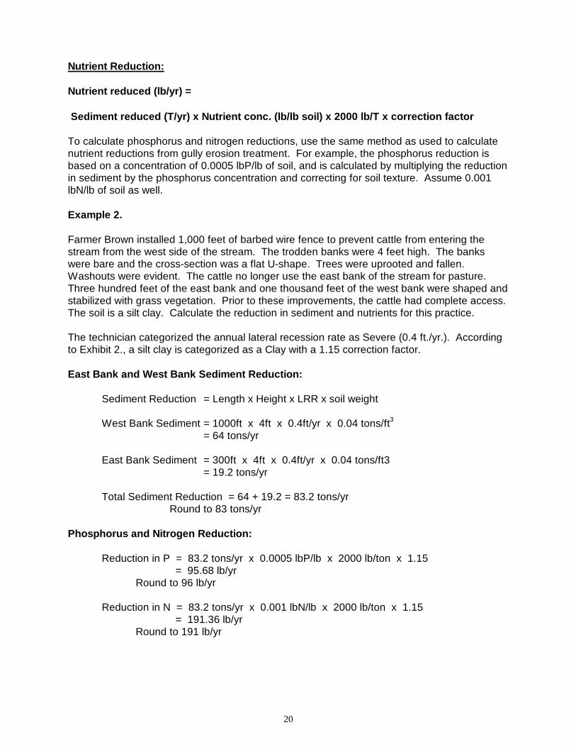
Nutrient Reduction:
Nutrient reduced (lb/yr) =
Sediment reduced (T/yr) x Nutrient conc. (lb/lb soil) x 2000 lb/T x correction factor
To calculate phosphorus and nitrogen reductions, use the same method as used to calculatenutrient reductions from gully erosion treatment. For example, the phosphorus reduction isbased on a concentration of 0.0005 lbP/lb of soil, and is calculated by multiplying the reductionin sediment by the phosphorus concentration and correcting for soil texture. Assume 0.001lbN/lb of soil as well.
Example 2.
Farmer Brown installed 1,000 feet of barbed wire fence to prevent cattle from entering thestream from the west side of the stream. The trodden banks were 4 feet high. The bankswere bare and the cross-section was a flat U-shape. Trees were uprooted and fallen.Washouts were evident. The cattle no longer use the east bank of the stream for pasture.Three hundred feet of the east bank and one thousand feet of the west bank were shaped andstabilized with grass vegetation. Prior to these improvements, the cattle had complete access.The soil is a silt clay. Calculate the reduction in sediment and nutrients for this practice.
The technician categorized the annual lateral recession rate as Severe (0.4 ft./yr.). Accordingto Exhibit 2., a silt clay is categorized as a Clay with a 1.15 correction factor.
East Bank and West Bank Sediment Reduction:
Sediment Reduction = Length x Height x LRR x soil weight
West Bank Sediment = 1000ft x 4ft x 0.4ft/yr x 0.04 tons/ft3
= 64 tons/yr
East Bank Sediment = 300ft x 4ft x 0.4ft/yr x 0.04 tons/ft3= 19.2 tons/yr
Total Sediment Reduction = 64 + 19.2 = 83.2 tons/yrRound to 83 tons/yr
Phosphorus and Nitrogen Reduction:
Reduction in P = 83.2 tons/yr x 0.0005 lbP/lb x 2000 lb/ton x 1.15= 95.68 lb/yr
Round to 96 lb/yr
Reduction in N = 83.2 tons/yr x 0.001 lbN/lb x 2000 lb/ton x 1.15= 191.36 lb/yr
Round to 191 lb/yr

21
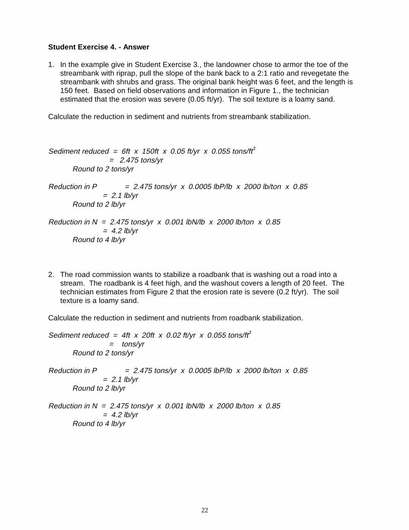
Student Exercise 4.
1. In the example give in Student Exercise 3., the landowner chose to armor the toe of thestreambank with riprap, pull the slope of the bank back to a 2:1 ratio and revegetate thestreambank with shrubs and grass. The original bank height was 6 feet, and the length is150 feet. Based on field observations and information in Figure 1., the technicianestimated that the erosion was severe (0.05 ft/yr). The soil texture is a loamy sand.
Calculate the reduction in sediment and nutrients from streambank stabilization.
2. The road commission wants to stabilize a roadbank that is washing out a road into astream. The roadbank is 4 feet high, and the washout covers a length of 20 feet. Thetechnician estimates from Figure 2 that the erosion rate is severe (0.2 ft/yr). The soiltexture is a loamy sand.
Calculate the reduction in sediment and nutrients from roadbank stabilization.
22
Student Exercise 4. - Answer
1. In the example give in Student Exercise 3., the landowner chose to armor the toe of thestreambank with riprap, pull the slope of the bank back to a 2:1 ratio and revegetate thestreambank with shrubs and grass. The original bank height was 6 feet, and the length is150 feet. Based on field observations and information in Figure 1., the technicianestimated that the erosion was severe (0.05 ft/yr). The soil texture is a loamy sand.
Calculate the reduction in sediment and nutrients from streambank stabilization.
Sediment reduced = 6ft x 150ft x 0.05 ft/yr x 0.055 tons/ft3
= 2.475 tons/yrRound to 2 tons/yr
Reduction in P = 2.475 tons/yr x 0.0005 lbP/lb x 2000 lb/ton x 0.85= 2.1 lb/yr
Round to 2 lb/yr
Reduction in N = 2.475 tons/yr x 0.001 lbN/lb x 2000 lb/ton x 0.85= 4.2 lb/yr
Round to 4 lb/yr
2. The road commission wants to stabilize a roadbank that is washing out a road into astream. The roadbank is 4 feet high, and the washout covers a length of 20 feet. Thetechnician estimates from Figure 2 that the erosion rate is severe (0.2 ft/yr). The soiltexture is a loamy sand.
Calculate the reduction in sediment and nutrients from roadbank stabilization.
Sediment reduced = 4ft x 20ft x 0.02 ft/yr x 0.055 tons/ft3
= tons/yrRound to 2 tons/yr
Reduction in P = 2.475 tons/yr x 0.0005 lbP/lb x 2000 lb/ton x 0.85= 2.1 lb/yr
Round to 2 lb/yr
Reduction in N = 2.475 tons/yr x 0.001 lbN/lb x 2000 lb/ton x 0.85= 4.2 lb/yr
Round to 4 lb/yr

23
IV. Agricultural Fields
This method will be used to calculate average annual sediment and attached phosphorus andnitrogen reductions following establishment of conservation practices such as these:
Prescribed GrazingResidue Management, Mulch TillConservation Crop RotationConservation CoverCover and Green ManureCritical Area PlantingStripcropping, ContourStripcropping, Field
The methods used to estimate the amount of sediment and nutrients that reach a waterbodyfrom upland areas differs significantly from the methods described earlier. We will first reviewsome of the concepts used to determine sediment delivery and the resulting amount ofsediment-borne nutrients.
One of the first steps in determining how much eroded soil reaches a water body is todetermine the contributing area. The contributing area is the portion of the priority field, whichcontributes eroded soil to the water body. The contributing area will usually differ in size fromthe priority field and is defined by the runoff flowpath and by topography. The flowpath is thedirection runoff flows, either towards or away from the edge of field adjacent to the hydrologicsystem (stream, lake, ditch, floodplain, wetland, etc.) that is being protected. The contributingarea may be larger than the priority field or smaller than it. See the diagrams below forexamples.
Figure 3. Contributing Area Examples
In both examples, the priority field is managed with appropriate Best Management Practices,but only the contributing area is used to calculate sediment and nutrient reductions.
24
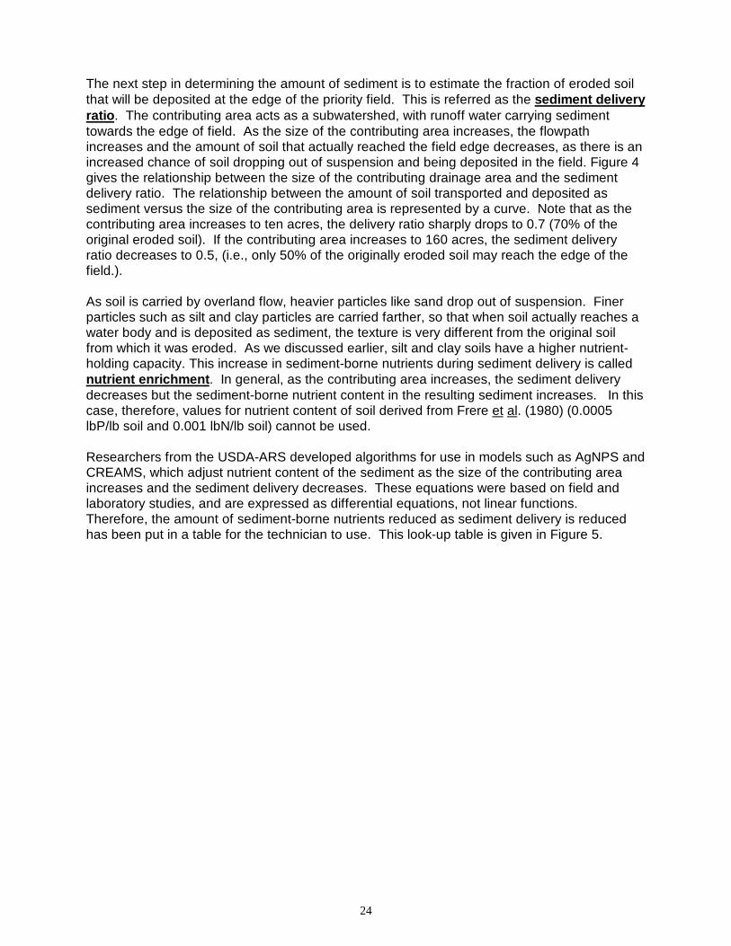
The next step in determining the amount of sediment is to estimate the fraction of eroded soilthat will be deposited at the edge of the priority field. This is referred as the sediment deliveryratio . The contributing area acts as a subwatershed, with runoff water carrying sedimenttowards the edge of field. As the size of the contributing area increases, the flowpathincreases and the amount of soil that actually reached the field edge decreases, as there is anincreased chance of soil dropping out of suspension and being deposited in the field. Figure 4gives the relationship between the size of the contributing drainage area and the sedimentdelivery ratio. The relationship between the amount of soil transported and deposited assediment versus the size of the contributing area is represented by a curve. Note that as thecontributing area increases to ten acres, the delivery ratio sharply drops to 0.7 (70% of theoriginal eroded soil). If the contributing area increases to 160 acres, the sediment deliveryratio decreases to 0.5, (i.e., only 50% of the originally eroded soil may reach the edge of thefield.).
As soil is carried by overland flow, heavier particles like sand drop out of suspension. Finerparticles such as silt and clay particles are carried farther, so that when soil actually reaches awater body and is deposited as sediment, the texture is very different from the original soilfrom which it was eroded. As we discussed earlier, silt and clay soils have a higher nutrient-holding capacity. This increase in sediment-borne nutrients during sediment delivery is callednutrient enrichment . In general, as the contributing area increases, the sediment deliverydecreases but the sediment-borne nutrient content in the resulting sediment increases. In thiscase, therefore, values for nutrient content of soil derived from Frere et al. (1980) (0.0005lbP/lb soil and 0.001 lbN/lb soil) cannot be used.
Researchers from the USDA-ARS developed algorithms for use in models such as AgNPS andCREAMS, which adjust nutrient content of the sediment as the size of the contributing areaincreases and the sediment delivery decreases. These equations were based on field andlaboratory studies, and are expressed as differential equations, not linear functions.Therefore, the amount of sediment-borne nutrients reduced as sediment delivery is reducedhas been put in a table for the technician to use. This look-up table is given in Figure 5.

25
Figure 4. Sediment Delivery Ratios Based on Contributing Drainage Area.

26
Figure 5. Phosphorus and Nitrogen Content of Sediment Delivered by Sheet and Rill Erosion.(Derived from AGNPS equations in Young et al, 1987).
27
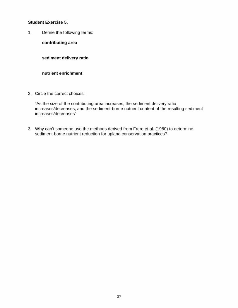
Student Exercise 5.
1. Define the following terms:
contributing area
sediment delivery ratio
nutrient enrichment
2. Circle the correct choices:
“As the size of the contributing area increases, the sediment delivery ratioincreases/decreases, and the sediment-borne nutrient content of the resulting sedimentincreases/decreases”.
3. Why can’t someone use the methods derived from Frere et al. (1980) to determinesediment-borne nutrient reduction for upland conservation practices?

28
Student Exercise 5. - Answers
1. Define the following terms:
contributing area: the portion of the priority field which contributes eroded soil to thewater body.
sediment delivery ratio: The fraction of eroded soil that will be deposited at the edge ofthe priority field.
nutrient enrichment: The increase in sediment-borne nutrients during sediment delivery.
2. Circle the correct choices:
“As the size of the contributing area increases, the sediment delivery ratioincreases/decreases , and the sediment-borne nutrient content of the resulting sedimentincreases /decreases”.
3. Why can’t someone use the methods derived from Frere et al. (1980) to determinesediment-borne nutrient reduction for upland conservation practices?
As soil moves across a land surface and sediment delivery decreases, nutrient enrichmenttakes place, and the values for nutrient content of soil derived from Frere et al. (1980)(0.0005 lbP/lb soil and 0.001 pbN/lb soil) cannot be used.

29
Sediment Reduction:
Sediment reduced (T/yr) = (B-A) x DR x CA
where B = sheet and rill erosion before treatment (T/ac/yr)A = sheet and rill erosion after treatment (T/ac/yr)DR = delivery ratio (a unitless fraction)CA = contributing area (acres)
There are four steps to calculating the sediment reductions from upland conservationpractices.
Step 1:Calculate the priority field’s soil being protected from sheet and rill erosion in tons per acre peryear. Section I of the Field Office Technical Guide instructs the technician on how to calculatewater erosion using the Revised Universal Soil Loss Equation (RUSLE) for the priority field(s).These computations can be reported as “Before” soil loss (“B”), the erosion in tons per acre peryear before the conservation practice(s); and the “After” soil loss (“A”), the erosion in tons peracre per year after the conservation practice(s). The differences between “B” and “A” is thereduction in soil loss in tons per acre per year as a result of installing conservation practices.
Step 2:Using professional judgement, determine the contributing area (CA) in acres.
Step 3:Using Figure 4, estimate the delivery ratio from the size of the contributing area. For example,a 14- acre contributing area would have a delivery ratio of 0.68.
Step 4:Calculate sediment reduced using the equation, (B-A) x DR x CA
Nutrient Reduction:
Step 1:Using Exhibit 2, classify the predominant soil texture from the soil texture triangle illustration.Exhibit 2 groups the various mineral soil classification textures into three families: clay, silt andsand. For example, a loamy clay would be classified as a Clay.
Step 2:Calculate the sediment-borne phosphorus and nitrogen using Figure 5. To utilize this graphproperly, sediment delivery reductions are calculated per acre and then the correspondingnutrient reduction is multiplied by the contributing area. First the “Before” soil loss (B) and the“After” soil loss (A) are individually multiplied by the delivery ratio to calculate the tons ofsediment delivered per acre per year. Then using Figure 5, the pounds per acre of nutrientsare determined. Next the pounds per acre of nutrients are multiplied by the contributing areafor the “B” situation and the “A” situation. Finally, the difference between the product of “B”and “A” is the reduction in nutrient.

30
Example:A farmer applied no-till to a 40- acre field directly adjacent to a stream. The soil is a clay loam,the “Before” soil loss is 10 t/ac/yr., and the “After” soil loss is 1 t/ac/yr. The techniciandetermines that the size of the contributing area is 25 acres. Calculate the sediment andsediment-borne phosphorus and nitrogen reduced from upland treatment of sheet and rillerosion.
Sediment Reduction:
Steps 1 and 2 are provided to the reader. B = 10 t/ac/yr. and A = 1 t/ac/yr.; and thecontributing area (CA) = 25 acres. Using Figure 4, a CA of 25 acres gives a delivery ratio (DR)of approximately 0.63
Reduction in Sediment Delivery = (B-A) x DR x CA= (10 - 1) x 0.63 x 25= 141.75 t/yr. Round to 142 t/yr.
Phosphorus Reduction:
a. “Before” sediment delivery (t/ac/yr) = DR x B= 0.63 x 10= 6.3 t/ac/yr. Round to 6 t/ac/yr
Using Exhibit 2, the clay loam is classified as a Clay.
b. From Figure 5, a sediment delivery of 6 t/ac/yr. has 7.71 lb/ac/yr. Attachedphosphorus.
c. Total “Before” phosphorus = attached P (from Figure 5) x CA= 7.71 lb/ac/yr x 25 ac.
= 192.75 lbs/yr
d. “After” sediment delivery (t/ac/yr) = DR x A= 0.63 x 1.0 t/ac/yr= 0.63 t/ac/yr. Round to 0.6 t/ac/yr
e. From Figure 5, 0.6 t/ac/yr sediment delivery has 1.22lb/ac attached phosphorus
f. Total “After” phosphorus = attached P (from Figure 5) x CA.= 1.22 lb/ac/yr x 25 ac.= 30.5 lb/yr
g. The reduction in phosphorus = 192.75 - 30.5 = 162.25 lb/yr Round to 162 lb P/yr
Nitrogen Reduction:
a. “Before” sediment delivery (t/ac/yr) = DR x B= 0.63 x 10= 6.3 t/ac/yr. Round to 6 t/ac/yr

31
Using Exhibit 2, the clay loam is classified as a Clay.
b. From Figure 5, a sediment delivery of 6 t/ac/yr has 15.42 lb/ac/yr attached nitrogen.c. Total “Before” nitrogen = attached N (from Figure 5) x CA
= 15.42 lb/ac/yr25 ac.= 385.5 lbs./yr
d. “After” sediment delivery (t/ac/yr) = DR x A= 0.63 x 1.0 t/ac/yr= 0.63 t/ac/yr. Round to 0.6 t/ac/yr
e. From Figure 5, 0.6 t/ac/yr sediment delivery has 2.44lb/ac/yr attached nitrogen.
f. Total “After” nitrogen = attached N (from Figure 5) x CA.= 2.44 lb/ac/yr x 25 ac.= 61 lb/yr
g. The reduction in nitrogen = 385.5 - 61 = 324.5 lb/yr Round to 325 lb N/yr.

32
Student Exercise 6 .
A landowner begins using mulch till on an 80- acre cornfield. The erosion rate before residuemanagement was 15 t/ac/yr, and the erosion rate after mulch till was 1.0 t/ac/yr. The soil typeis a silty clay loam. Using field observations, the technician determines that the contributingarea is only 30 acres. Calculate the sediment and phosphorus reduction from conversion tomulch till.
33
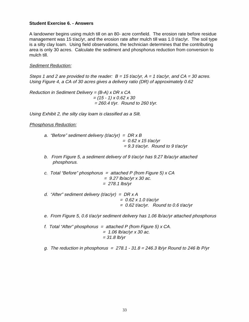
Student Exercise 6. - Answers
A landowner begins using mulch till on an 80- acre cornfield. The erosion rate before residuemanagement was 15 t/ac/yr, and the erosion rate after mulch till was 1.0 t/ac/yr. The soil typeis a silty clay loam. Using field observations, the technician determines that the contributingarea is only 30 acres. Calculate the sediment and phosphorus reduction from conversion tomulch till.
Sediment Reduction:
Steps 1 and 2 are provided to the reader: B = 15 t/ac/yr, A = 1 t/ac/yr, and CA = 30 acres.Using Figure 4, a CA of 30 acres gives a delivery ratio (DR) of approximately 0.62
Reduction in Sediment Delivery = (B-A) x DR x CA= (15 - 1) x 0.62 x 30= 260.4 t/yr. Round to 260 t/yr.
Using Exhibit 2, the silty clay loam is classified as a Silt.
Phosphorus Reduction:
a. “Before” sediment delivery (t/ac/yr) = DR x B= 0.62 x 15 t/ac/yr= 9.3 t/ac/yr. Round to 9 t/ac/yr
b. From Figure 5, a sediment delivery of 9 t/ac/yr has 9.27 lb/ac/yr attachedphosphorus.
c. Total “Before” phosphorus = attached P (from Figure 5) x CA= 9.27 lb/ac/yr x 30 ac.
= 278.1 lbs/yr
d. “After” sediment delivery (t/ac/yr) = DR x A= 0.62 x 1.0 t/ac/yr= 0.62 t/ac/yr. Round to 0.6 t/ac/yr
e. From Figure 5, 0.6 t/ac/yr sediment delivery has 1.06 lb/ac/yr attached phosphorus
f. Total “After” phosphorus = attached P (from Figure 5) x CA.= 1.06 lb/ac/yr x 30 ac.= 31.8 lb/yr
g. The reduction in phosphorus = 278.1 - 31.8 = 246.3 lb/yr Round to 246 lb P/yr

34
V. Filter Strips
Many watershed projects have filter strip programs. Filter strips further reduce the sedimentand nutrient loads delivered to the surface water from upland sources. The relative grosseffectiveness of filter strips for sediment reduction is 65%; for phosphorus is 75%; andfor nitrogen is 70% (Pennsylvania State University, 1992).
Sediment ReductionTo calculate the added reduction of sediment, the “after” soil loss (A) is adjusted to reflect theadded 65% reduction. For example, if A without a filter strip is 1 ton/ac/yr, inclusion of a filterstrip would reduce sediment delivery to 0.35 ton/ac/yr (0.35 x 1). In other words, if 65%sediment reduction takes place, then 35% is left, which is expressed as a fraction (0.35). Theresulting reduction in sediment [(B-A) x DR x CA] is the combined sediment reduction fromboth the filter strip and upland treatment.
Example:Farmer Brown adopted no-till and reduced sediment delivery by 86 t/yr, phosphorus by 103 lb.and nitrogen by 205 lb. B = 10 t/ac/yr., and A = 1 t/ac/yr. Soil type is clay loam. CA = 14acres. If Farmer Brown installs filter strips along Clear Creek along with the no-till, what wouldbe the reduction in sediment and nutrients?
Sediment Reduction
= [tons Before – (fraction delivered to stream x tons After)] x DR x CA
= (10 - (0.35 x 1)) x 0.68 x 14
= 91.8 t/yr. Round to 92 t/yr
The 92 t/yr is the reduction in sediment load from the filter strip and no-till combined. Tocalculate the reduction in sediment from the filter strip alone:
92t/yr – 86t/yr = 6 t/yr.
Nutrient Reduction
To calculate the additional reduction in nutrients (phosphorus and nitrogen), the “After” soilloss (A) is adjusted to reflect the additional reduction of 75% for phosphorus and of 70% fornitrogen. For example, the “after” soil loss for phosphorus for the combined filter strip andupland treatment would be 0.25 multiplied by the original (upland treatment only) “after” soilloss. The “after” soil loss for nitrogen from both a filter strip and upland treatment would be0.30 multiplied by the original “after” soil loss. Calculation of the “Before” soil loss (B) is thesame as for other upland erosion treatments. The “After” soil loss (A) is adjusted as shown inthe example below. The difference between the product of “B” and “A” is the combinedreduction in nutrient from the filter strip and upland treatment.
Phosphorus Reduction :
a. “Before” soil loss:0.68 x 10 t/ac/yr. = 6.8 t/ac/yr; Round to 7 t/ac/yr
35
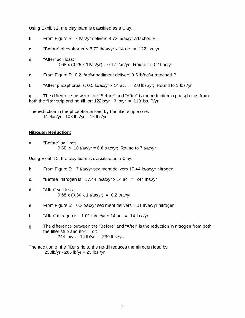
Using Exhibit 2, the clay loam is classified as a Clay.
b. From Figure 5: 7 t/ac/yr delivers 8.72 lb/ac/yr attached P
c. “Before” phosphorus is 8.72 lb/ac/yr x 14 ac. = 122 lbs./yr
d. “After” soil loss:0.68 x (0.25 x 1t/ac/yr) = 0.17 t/ac/yr; Round to 0.2 t/ac/yr
e. From Figure 5: 0.2 t/ac/yr sediment delivers 0.5 lb/ac/yr attached P
f. “After” phosphorus is: 0.5 lb/ac/yr x 14 ac. = 2.8 lbs./yr; Round to 3 lbs./yr
g,. The difference between the “Before” and “After” is the reduction in phosphorus fromboth the filter strip and no-till, or: 122lb/yr - 3 lb/yr = 119 lbs. P/yr
The reduction in the phosphorus load by the filter strip alone:119lbs/yr - 103 lbs/yr = 16 lbs/yr
Nitrogen Reduction :
a. “Before” soil loss:0.68 x 10 t/ac/yr = 6.8 t/ac/yr; Round to 7 t/ac/yr
Using Exhibit 2, the clay loam is classified as a Clay.
b. From Figure 5: 7 t/ac/yr sediment delivers 17.44 lb/ac/yr nitrogen
c. “Before” nitrogen is: 17.44 lb/ac/yr x 14 ac. = 244 lbs./yr
d. “After” soil loss:0.68 x (0.30 x 1 t/ac/yr) = 0.2 t/ac/yr
e. From Figure 5: 0.2 t/ac/yr sediment delivers 1.01 lb/ac/yr nitrogen
f. “After” nitrogen is: 1.01 lb/ac/yr x 14 ac. = 14 lbs./yr
g. The difference between the “Before” and “After” is the reduction in nitrogen from boththe filter strip and no-till, or:
244 lb/yr. - 14 lb/yr = 230 lbs./yr.
The addition of the filter strip to the no-till reduces the nitrogen load by:230lb/yr - 205 lb/yr = 25 lbs./yr.

36
Student Exercise 7 .
The landowner from Student Exercise 6 installs a filter strip at the edge of the 80- acrecornfield along a county drain and continues to apply residue management in the cornfield.The erosion rate was 15 t/ac/yr, and the erosion rate after establishment of the filter strip andresidue management was 1.0 t/ac/yr. The soil type is a silty clay loam. Using fieldobservations, the technician determines that the contributing area is only 30 acres. Calculatethe sediment and phosphorus reduction from the combined filter strip and upland treatment.What amount of sediment and phosphorus is due to the filter strip alone?

37
Student Exercise 7. - Answers
The landowner from Student Exercise 6 installs a filter strip at the edge of the 80- acrecornfield along a county drain and continues to apply residue management in the cornfield.The erosion rate was 15 t/ac/yr, and the erosion rate after establishment of the filter strip andresidue management was 1.0 t/ac/yr. The soil type is a silty clay loam. Using fieldobservations, the technician determines that the contributing area is only 30 acres. Calculatethe sediment and phosphorus reduction from the combined filter strip and upland treatment.What amount of sediment and phosphorus is due to the filter strip alone?
Sediment Reduction (residue management plus filter strip):
Steps 1 and 2 are provided to the reader: B = 15 t/ac/yr, A = 1 t/ac/yr, and CA = 30 acres.Using Figure 4, a CA of 30 acres gives a delivery ratio (DR) of approximately 0.62. Thereductions of sediment from residue management is 260 t/yr., and 246 lb/yr. Phosphorus(answer to Student Exercise 6).
Sediment reduced = (15 - (0.35 x 1)) x 0.62 x 30= 272.49 t/yr. Round to 272.
The amount of sediment reduced from the filter strip alone is 272 t/yr – 260 t/yr = 12 t/yr.
Phosphorus Reduction (residue management plus filter strip):
a. “Before” soil loss:0.62 x 15 t/ac/yr. = 9.3 t/ac/yr; Round to 9 t/ac/yr
Using Exhibit 2, the clay loam is classified as a Clay.
b. From Figure 5: 9 t/ac/yr delivers 10.7 lb/ac/yr attached P
c. “Before” phosphorus is 10.7 lb/ac/yr x 30 ac. = 321 lbs./yr.
d. “After” soil loss:0.62 x (0.25 x 1t/ac/yr) = 0.15 t/ac/yr; Round to 0.2 t/ac/yr
e. From Figure 5: 0.2 t/ac/yr sediment delivers 0.5 lb/ac attached P
f. “After” phosphorus is: 0.5 lb/ac/yr x 30 ac. = 15 lbs./yr
g,. The difference between the “Before” and “After” is the reduction in phosphorus fromboth the filter strip and no-till, or: 321lb/yr - 15 lb/yr. = 306 lbs./yr.
The reduction in the phosphorus load by the filter strip: 306lbs/yr. - 246 lbs/yr. = 60 lbs/yr.

38
FEEDLOT POLLUTION REDUCTION
An animal lot refers to an open lot or combination of open lots intended for confined feeding,breeding, raising or holding animals. It is specifically designed as a confinement area in whichmanure accumulates or where the concentration of animals is such that vegetation cannot bemaintained.
Runoff from feedlots contains many agents that can be considered potential pollutants,including disease carrying organisms, organic matter, nutrients and suspended inorganicsolids. These agents affect receiving waters by increasing the nutrient and suspended solidconcentration, decreasing dissolved oxygen content of water, and in some cases, eventhreaten human and animal health. For nonpoint source watershed project progress reporting,we have selected chemical oxygen demand (COD) and phosphorus (P) as representativepollutant indicators to represent pollutant reduction.
Chemical Oxygen Demand (COD) is a measure of the amount of oxygen required to oxidizeorganic and oxidizable inorganic compounds in water. It can be used as a lumped parameterthat reasonably appears to represent the degree of pollution in effluent. Phosphorus (P) isfound in animal manure and is a major contributor to eutrophication of surface waters and istherefore an important pollutant indicator.
The purpose of these calculations is to represent the COD and P reductions after an animalwaste system is installed. This method has two assumptions: 1) the feedlot is adjacent to areceiving hydrologic system without any buffering areas; and 2) installing the animal wastesystem will prevent any further pollutants from the lot from reaching the hydrologic system.Therefore the mass load of the COD and P calculated for the before situation will be thereduction in pollutants.
There may be feedlot sites where small buffers between the feedlot and waterbody alreadyexist. Each of these situations should be handled individually with NPS Staff assistance.Feedlots that cannot show impact to the hydrologic system being protected should not beevaluated with this computation. An example of this would be a feedlot that does not haverunoff reaching the hydrologic system, but is receiving technical assistance in order that wasteutilization can be applied at agronomic rates. In this case, the impact would be reported usingthe ICM report for priority fields.
There are 12 steps involved in this calculation process. Use the worksheet given as Exhibit 3in the Appendix as we go through the following example.
Example: Farmer Brown milks 70 dairy cows and has 30 replacement cows and 30 youngstock. All the animals are confined in 80% paved feedlot. The feedlot is adjacent to ClearCreek and discharges into it. Determine the reduction in COD and P for the feedlot after theWaste Management System is installed.

39
The following steps will calculate the COD and P loading reductions for installation of theWaste Management System.
Step 1: Carefully study the animal lot before the installation of the Waste ManagementSystem. Briefly describe the discharge point(s) using the name of the receivingwater. All calculations will be based on feedlot situation before anyimprovements were made.
Step 2: On the back of the worksheet, sketch the feedlot. (Figure 6 gives a sketch ofFarmer Brown’s feedlot.) From field measurements determine the perimeterdimensions of the area contributing polluted water to the discharge point(s).This is the contributing area (CA). If the lot was partly paved and partlyearthen, determine the proportion of the total that is paved.
Contributing Area (CA) = 75,620 ft2 X 1 ac/43560 ft2 = 1.74 acPercent paved = 80%
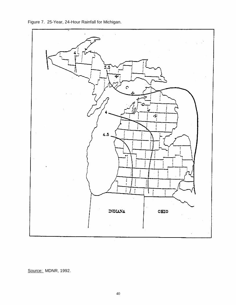
Step 3: Determine the design rainfall (R) from the rainfall map, Figure 7, for a 25-year,24-hour rainfall. Federal regulations governing discharge of surface runoff fromanimal lots require 25-year, 24-hour storm events. This is consistent with NRCSstandards and specifications.
R = 4.0 inches
Step 4: Determine the soil cover complex number (CN) for the feedlot based onFigure 8.
Figure 8. Curve Numbers for Feedlots
Percent Paved 0 – 24% 25 – 49% 50 – 74% 75 – 100%CN 91 92 93 94
In this example, CN = 94
40
Figure 7. 25-Year, 24-Hour Rainfall for Michigan.
Source: MDNR, 1992.

41
Step 5:Enter the number of animals in the lot and the animal type factors from Figure 9 for theCOD and P. Animal types, number and weights utilized in this step should beconsistent with those used in the design for the animal waste storage system.Interpolation of values should be based on the maximum weight animals would beexpected to reach.
Animal TypeDairy Cow Number of Animals = 100 Young Dairy Number of Animals = 30
COD factor = 1.96 COD factor = 0.70P factor = 0.92 P factor = 0.33
Figure 9. Ratio of Chemical Oxygen Demand (COD) and total phosphorus (P) produced byvarious animals to that produced by a 1,000 pound slaughter steer.
AnimalType
DesignWeight1
CODRatio
PRatio
PoundsSlaughter Steer 1,000 1.00 1.00
Young Beef 500 .50 .51Dairy Cow 1,400 1.96 .92
Young Dairy Stock 500 .70 .33Swine 200 .17 .27
Feeder Pig 50 .04 .07Sheep 100 .18 .06Turkey 10 .02 .03
Chicken 4 .01 .01Duck 4 .01 .01Horse 1,000 .42 .42
Step 6:Calculate the runoff using the following equations:
S = 1000 - 10 Q = (R-0.2S)2
CN R + 0.8S
where S = an empirical model coefficientCN = soil cover complex number (Step 4)R = design rainfall in inches (Step 3)Q = runoff in inches
S = 1000 - 10 Q = [4.0 - 0.2(0.6383)]2
94 4.0 + 0.8(.0.6383)
S = 0.6383 Q = 3.32 in.

42
Step 7:Calculate the runoff volume (V) using the following equation:
V = Q x CA
where V = runoff volume in acre-inchesQ = runoff in inches (Step 6)CA = contributing area in acres (Step 2)
V = 3.32 x 1.74 = 5.78 acre-in.
Step 8:Because animal species differ in their relative production of wastes, thisstep equates amount of waste to the standard 1000 lb. feeder steer. Thusthe amount of pollutant produced by a beef animal is represented as one,with the amount produced by all other animals being a fraction relative tothat. Calculate the equivalent animal unit (EAU) for COD and P usinginformation from Step 5 in the following equation:
No. x Factor = EAU
where No. = number of animals (Step 5)Factor = ratio of COD and P produced (Step 5)
Animal Type No. of Animals x Factor = EAU
COD: Dairy Cow 100 x 1.96 = 196.0Young Dairy 30 x 0.70 = 21.0
P: Dairy Cow 100 x 0.92 = 92.0Young Dairy 30 x 0.33 = 9.9
Step 9:When animal density is high, such as in a confined feedlot, almost all ofthe rainfall and runoff in and from the lot comes in contact with animalwaste before leaving the lot. When animal density is low, some runoffmay escape contact with manure and thus not be contaminated. Calculatethe Animal Unit Density (AUD) and percent manure pack using thefollowing equations:
EAU / CA = AUD
where EAU = Equivalent Animal Units (step 8)CA = contributing area (Step 2)
If AUD < 100, percent manure pack = AUD;If AUD > 100, percent of manure pack = 100%.
The assumption is that AUDs greater than 100 have a pollutant concentration that reaches amaximum level independent of the number of animal units.
COD: 217.0 / 1.74 = 124.7 AUD; assume manure pack = 100%P: 101.9 / 1.74 = 58.6 AUD; manure pack = 58.6%
43
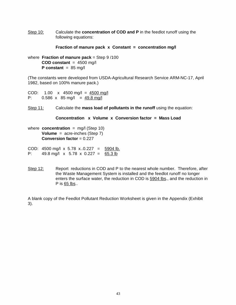
Step 10: Calculate the concentration of COD and P in the feedlot runoff using thefollowing equations:
Fraction of manure pack x Constant = concentration mg/l
where Fraction of manure pack = Step 9 /100COD constant = 4500 mg/lP constant = 85 mg/l
(The constants were developed from USDA-Agricultural Research Service ARM-NC-17, April1982, based on 100% manure pack.)
COD: 1.00 x 4500 mg/l = 4500 mg/lP: 0.586 x 85 mg/l = 49.8 mg/l
Step 11: Calculate the mass load of pollutants in the runoff using the equation:
Concentration x Volume x Conversion factor = Mass Load
where concentration = mg/l (Step 10)Volume = acre-inches (Step 7)Conversion factor = 0.227
COD: 4500 mg/l x 5.78 x..0.227 = 5904 lb.P: 49.8 mg/l x 5.78 x 0.227 = 65.3 lb
Step 12: Report reductions in COD and P to the nearest whole number. Therefore, afterthe Waste Management System is installed and the feedlot runoff no longerenters the surface water, the reduction in COD is 5904 lbs., and the reduction inP is 65 lbs..
A blank copy of the Feedlot Pollutant Reduction Worksheet is given in the Appendix (Exhibit3).
44
INTEGRATED CROP MANAGEMENT REPORTING FOR PESTICIDES, COMMERCIALFERTILIZER, and MANURE UTILIZATION
Section 319 watershed projects are required to practice Integrated Crop Management (ICM) onall priority fields. The Water Quality Resource Management Plan (WQRMP) must include ICMas a required component for the landowner to be eligible for cost-share on other practicesusing 319 funds. The WQRMP should reference the ICM plan.
The goal of ICM is to improve the management practices used by the producer, to bring thelevel of management to another level for better water quality protection. For example, aproducer who is not currently using soil tests on the priority fields would include soil testing inhis/her ICM plan. A producer who is currently using soil tests to set yield goals couldincorporate other nutrient management techniques such as nitrate testing, split application offertilizer, or other practices to better manage nutrients. The Water Quality ResourceManagement Plan (WQRMP) must include ICM as a required practice for cost-share eligibility,and should reference the ICM plan.
An ICM plan should be prepared for priority fields, documenting the pest and nutrientmanagement practices that the landowner is implementing on these fields. The ICM plan is tobe customized to the individual farm plan for the watershed’s targeted pollutants. For example,if the watershed is to reduce sediment and phosphorus from entering the stream, the ICM planwould specify what ICM practices the landowner is using to address phosphorus. An ICM planwould differ for a livestock producer, cash crop producer, or a fruit producer.
A livestock producer’s ICM plan would emphasize manure utilization and fertilizermanagement. Pesticide management would not include time and effort consuming activitiessuch as scouting. However, the WQRMP would reference Pesticide Management as requiringthe farmer to follow pesticide label restrictions and directions.
A cash crop farmer’s ICM plan would include both integrated pest and fertilizer management.Integrated Pest Management (IPM) would be planned and applied depending on thetechnician’s overall workload and availability. The technician may delegate IPM planning andtraining to MSU Extension personnel or private consultants. Or the technician may organizeIPM training for participants in the watershed as a method of applying pest management. (Itshould be noted that EPA rules prohibit the use of 319 funds to fund ICM practices. Incentivefunds may be available through the USDA’s Environmental Quality Incentives Program.)
A fruit producer’s ICM plan would include both IPM and fertilizer management.
The format for ICM plans and documentation is not formalized in water quality projects. Thedocuments should be understandable by the producers, so that they understand whatpractices are required and how they are carried out. Documentation in the WQRMP should bespecific enough for a reviewer to assess what practices are being used, when they arescheduled for implementation, and that they have been applied properly to meet water qualitygoals. The MSU Extension service and private firms offer forms and computer programs forproducing ICM plans.
Attempts to quantify water quality impacts of ICM have been largely ineffective. Progressreporting has largely been based on tracking the number and acres of ICM practices applied topriority fields. Attached is an example of an ICM quarterly summary report, to document ICMactivities within the watershed project. Progress is cumulative for the entire project and is to bereported with quarterly reports. For example, if at the end of the first quarter the project had

45
three participants and added one participant in the second quarter, the project’s current statusis four participants. Therefore 1a of the Integrated Crop Management Quarterly Report for theSecond Quarter would be 4 (Figures 10 and 11). The second and subsequent year progressis accumulated in the same manner. Progress is never double or triple counted on the samepeople or acres.
Some projects have found the Individual Farm ICM Quarterly Summary to be an effectivemeans to keep records of priority fields. Each participant has an ICM record sheet so that thetechnician may track progress. This can be kept in the case file or in a separate notebookspecific to 319 ICM.
A blank copy of the ICM Quarterly Report is given as Exhibit 4 in the Appendix.
46
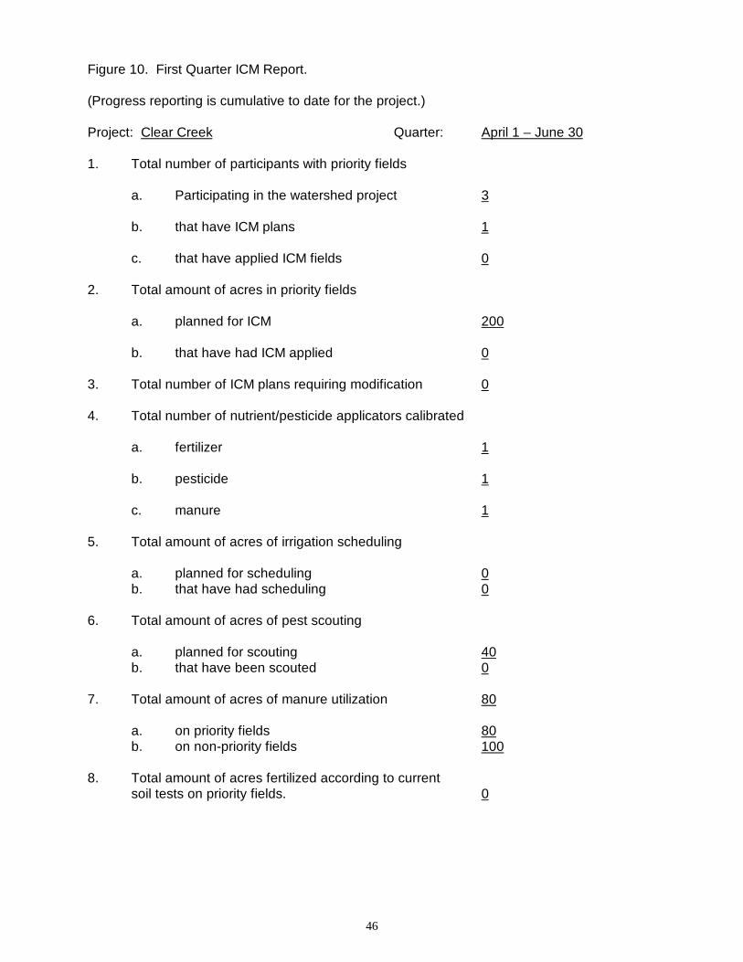
Figure 10. First Quarter ICM Report.
(Progress reporting is cumulative to date for the project.)
Project: Clear Creek Quarter: April 1 – June 30
1. Total number of participants with priority fields
a. Participating in the watershed project 3
b. that have ICM plans 1
c. that have applied ICM fields 0
2. Total amount of acres in priority fields
a. planned for ICM 200
b. that have had ICM applied 0
3. Total number of ICM plans requiring modification 0
4. Total number of nutrient/pesticide applicators calibrated
a. fertilizer 1
b. pesticide 1
c. manure 1
5. Total amount of acres of irrigation scheduling
a. planned for scheduling 0b. that have had scheduling 0
6. Total amount of acres of pest scouting
a. planned for scouting 40b. that have been scouted 0
7. Total amount of acres of manure utilization 80
a. on priority fields 80b. on non-priority fields 100
8. Total amount of acres fertilized according to currentsoil tests on priority fields. 0

47
Figure 11. Second Quarterly ICM Report.
(Progress reporting is cumulative to date for the project.)
Project: Clear Creek Quarter: July 1 – September 31
1. Total number of participants with priority fields
a. Participating in the watershed project 4
b. that have ICM plans 3
c. that have applied ICM fields 0
2. Total amount of acres in priority fields
a. planned for ICM 320
b. that have had ICM applied 0
3. Total number of ICM plans requiring modification 0
4. Total number of nutrient/pesticide applicators calibrated
a. fertilizer 1
b. pesticide 1
c. manure 1
6. Total amount of acres of irrigation scheduling
a. planned for scheduling 0b. that have had scheduling 0
6. Total amount of acres of pest scouting
a. planned for scouting 80b. that have been scouted 0
7. Total amount of acres of manure utilization
a. on priority fields 160b. on non-priority fields 200
9. Total amount of acres fertilized according to currentsoil tests on priority fields. 0

48
GLOSSARY
Best Management Practice (BMP) : structural, vegetative or management conservationpractices which reduce or prevent detachment, transport and delivery of nonpoint sourcepollutants to surface or ground waters.
Channel Erosion Equation (CEE) : a formula to calculate the soil loss from streambankerosion, erosion from road stream crossings, or other similar types of erosion.
Contributing Area (CA) : the portion of the priority field, which contributes eroded soil to thewater body.
Erosion : the wearing away or disintegration of earth material by the physical forces of movingwind and water.
Gully Erosion Equation (GEE) : a formula to calculate the soil loss from concentrated flow,gullies or other similar types of erosion
Integrated Crop Management (ICM) : a system of pest and nutrient management practicesthat will minimize entry of nutrients, manure and/or pesticides to surface and ground waterwhile optimizing crop and forage yields.
Integrated Pest Management (IPM) : a system of chemical, physical and biological practicesto control pests, that will minimize entry of pesticides to surface and ground water whileoptimizing crop and forage yields.
Lateral Recession Rate (LRR) : the thickness of soil eroded from a bank surface(perpendicular to the face) in an average year, given in feet per year. Used in the ChannelErosion Equation.
Nutrient enrichment : the increase in sediment-borne nutrients during sediment delivery.
Priority field : cropland, pastureland or hayland that contribute runoff to adjacent hydrologicsystems such as lakes, streams, ditches, wetlands and flood plains.
Revised Universal Soil Loss Equation (RUSLE) : an erosion model predicting long-term,average annual soil loss resulting from raindrop splash and runoff from specific field slopes inspecified cropping and management systems and from rangeland.
Riparian : of or pertaining to the edge of a water body
Sediment delivery : the amount or fraction of earth material that is actually delivered to awater body.
Sediment Delivery Ratio (DR) : the fraction of eroded soil that will be deposited at the edge ofthe priority field. Used in equations to calculate sediment and nutrient reduction from uplandBMPs.
Soil loss tolerance : a measure of the amount of soil that can be removed from a site beforesoil productivity onsite is affected.

49
Water Quality Resource Management Plan (WQRMP) : a record of the BMPs chosen by thelandowner, which will address the sources of pollutants.

50
TECHNICAL REFERENCES
Frere, M.H., Ross, J.D., and Lane, L.J. 1980. The nutrient submodel. In: Knisel, W., ed.,CREAMS, A Field Scale Model for Chemicals, Runoff and Erosion From AgriculturalManagement Systems. U.S. Dept. Agric. Cons. Res. Report 26, vol. 1, ch. 4, p. 65-86.
Michigan Department of Natural Resources, Land and Water Management Division. 1992.Stormwater Management Guidebook.
Pennsylvania State University. 1992. Nonpoint Source Database. page 2-15 In: U.S. EPA,Guidance Specifying Management Measures For Sources of Nonpoint Source Pollution inCoastal Waters.
Steffen, L.J., 1982. Channel Erosion. personal communication.
U.S. Department of Agriculture. Natural Resources Conservation Service. Field OfficeTechnical Guide for Michigan. Section I-C. Water Erosion Prediction.
Young, R.A., C.A. Onstad, D.D. Bosch, and W.P. Anderson, 1987. AGNPS, Agricultural –Non-Point-Source Pollution Model; A Large Watershed Analysis Tool. U.S. Department ofAgriculture – Agriculture Res. Serv., Conservation Resource Report 35, Washington, D.C.,
pp. 77.
51
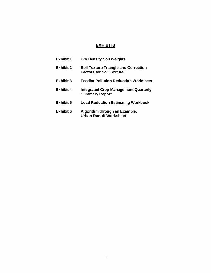
EXHIBITS
Exhibit 1 Dry Density Soil Weights
Exhibit 2 Soil Texture Triangle and Correction Factors for Soil Texture
Exhibit 3 Feedlot Pollution Reduction Worksheet
Exhibit 4 Integrated Crop Management Quarterly
Summary Report
Exhibit 5 Load Reduction Estimating Workbook
Exhibit 6 Algorithm through an Example: Urban Runoff Worksheet

52
Exhibit 1Dry Density Soil Weights
SOIL TEXTURAL CLASS DRY DENSITY
Tons/Ft3
Sands, loamy sands .055
Sandy Loam .0525
Fine sandy loam .05
Loams, sandy clay loams, sandy clay .045
Silt loam .0425
Silty clay loam, silty clay .04
Clay loam .0375
Clay .035
Organic .011

53
Exhibit 2Soil Texture Triangle
Correction Factors for Soil Texture
Soil Texture Correction FactorClay 1.15Silt 1.00
Sand .85Peat 1.50
54
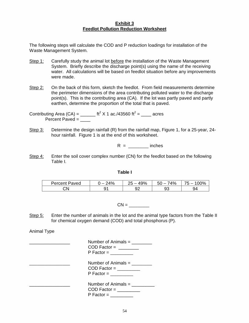
Exhibit 3Feedlot Pollution Reduction Worksheet
The following steps will calculate the COD and P reduction loadings for installation of theWaste Management System.
Step 1: Carefully study the animal lot before the installation of the Waste ManagementSystem. Briefly describe the discharge point(s) using the name of the receivingwater. All calculations will be based on feedlot situation before any improvementswere made.
Step 2: On the back of this form, sketch the feedlot. From field measurements determinethe perimeter dimensions of the area contributing polluted water to the dischargepoint(s). This is the contributing area (CA). If the lot was partly paved and partlyearthen, determine the proportion of the total that is paved.
Contributing Area (CA) = ______ ft2 X 1 ac./43560 ft2 = ____ acresPercent Paved = ____
Step 3: Determine the design rainfall (R) from the rainfall map, Figure 1, for a 25-year, 24-hour rainfall. Figure 1 is at the end of this worksheet.
R = ________ inches
Step 4: Enter the soil cover complex number (CN) for the feedlot based on the followingTable I.
Table I
Percent Paved 0 – 24% 25 – 49% 50 – 74% 75 – 100%CN 91 92 93 94
CN = ________
Step 5: Enter the number of animals in the lot and the animal type factors from the Table IIfor chemical oxygen demand (COD) and total phosphorus (P).
Animal Type
________________ Number of Animals = ________COD Factor = ________P Factor = _________
________________ Number of Animals = ________COD Factor = _________P Factor = _________
________________ Number of Animals = _________COD Factor = _________P Factor = _________

55
Table II
Ratio of COD and P produced by various animals to that produced by a 1,000 pound slaughtersteer.
AnimalType
DesignWeight1
CODRatio
PRatio
PoundsSlaughter Steer 1,000 1.00 1.00
Young Beef 500 .50 .51Dairy Cow 1,400 1.96 .92
Young Dairy Stock 500 .70 .33Swine 200 .17 .27
Feeder Pig 50 .04 .07Sheep 100 .18 .06Turkey 10 .02 .03
Chicken 4 .01 .01Duck 4 .01 .01Horse 1,000 .42 .42
1Interpolation of values should be based on the maximum weight animals would be expectedto reach.
Step 6: Calculate the runoff using the following equations:
S = 1000 – 10 Q = (R-0.2S)2
CN R + 0.8SWere S = an emp
CN = soil cover complex number (Step 4)R = design rainfall in inches (Step 3)Q = runoff in inches
Q = _________ inches
Step 7: Calculate the runoff volume (V) using the following equation:
V = Q X CA
Where V = runoff volume in acre-inchesQ = runoff in inches (Step 6)CA = contributing area of acres (Step 2)
V = ___________ X ___________V = ___________ acre-in
Step 8:Calculate the equivalent animal units (EAU) for COD and P using information from Step5 using the following equation:
No. X Factor = EAU
Where No. = Number of Animals (Step 5)Factor = ratio of COD and P produced (Step 5)

56
Animal Type No. of Animals x Factor = EAU
COD: __________ __________ x _______ = _____________
__________ __________ x _______ = _____________
__________ __________ x _______ = _____________
TOTAL = _____________
Step 9: Calculate the Animal Unit Density (AUD) and % manure pack using the followingequation:
EAU - CA = AUD
EAU = (Step 8)CA = (Step 2)
COD: ________ - ________ = ________ AUD*
P: ________ - ________ = ________ AUD*
* If AUD < 100, percent manure pack = AUDIf AUD > 100, percent manure pack = 100%
Manure pack (COD) = ________%
Manure pack (P) = ________%
Step 10: Calculate the concentration of COD and P in the feedlot runoff using the followingequations:
Fraction of manure pack x Constant = concentration mg/l
Fraction of manure pack = Step 9/100COD Constant* = 4500 mg/lP Content* = 85 mg/l
*Constants developed from USDA-Agricultural Research Service, ARM-NC-17 April1982, based on 100% manure pack.
COD: ________ X 4500mg/l = ________mg/l
P: ________ X 85 mg/l = ________mg/l
Step11: Calculate the mass load of pollutants in the runoff using the following equation:
Concentration X Volume X Conversion Factor = Mass Load
Concentration = mg/l (Step 10)Volume = acre-inches (Step 7)

57
Conversion factor = 0.227
COD ________ X ________ X 0.227 = ________ lb.
P ________ X ________ X 0.227 = ________ lb.
Step 12: Therefore, after the Waste Management System is installed and the feedlot runoff nolonger enters the surface water, the reduction in COD is _______ lbs. and thereduction in P is _______ lbs.

58
Figure 1. 25-Year, 24-Hour Rainfall for Michigan
Source: MDNR, 1992.

59
Exhibit 4INTEGRATED CROP MANAGEMENT QUARTERLY SUMMARY REPORT
(Progress reporting is cumulative to date for the project.)
Project _____________________________ Quarter ___________________________
1) Total number of participants with priority fields
a. Participating in the watershed project ________b. that have ICM plans ________c. that have applied ICM plans ________
2) Total amount of acres in priority fields
a. planning for ICM ________b. that have had ICM applied ________
3) Total number of ICM plans requiringModification ________
4) Total number of nutrient/pesticide applicators calibrated
a. fertilizerb. pesticidec. manure
5) Total amount of acres of irrigation scheduling
a. planned for scheduling ________b. that have had scheduling ________
6) Total amount of acres of pest scouting
a. planned for scouting ________b. that have been scouted ________
7) Total amount of acres of manure utilization
a. on priority fields ________b. on non-priority fields ________
8) Total amount of acres fertilized according toCurrent soil tests on priority fields -------

60
Exhibit 5 Load Reduction Estimating Workbook
A load reduction estimating workbook in Microsoft Excel® has been developed based on this document to provide a gross estimate of sediment and nutrient load reductions from the implementation of agricultural best management practices (BMPs). The methodology for the gross estimate of sediment and other constituent load reductions from the implementation of urban BMPs is based on reduction efficiencies and calculations developed by Illinois Environmental Protection Agency. The original version (developed in 1999) of the load reduction estimating workbook was comprised of the following worksheets:
• Introductions • Gully Stabilization • Bank Stabilization • Agricultural Fields and Filter Strips • Feedlots • Urban Runoff
A new worksheet—CountyData—was added to the workbook in 2002. The CountyData worksheet contains a collection of state and county names, precipitation data (annual amount and number of rain days) and correction factors (rainfall and number of rain days were adjusted to account for the runoff-producing events only), and USLE parameter values summarized from the 1997 National Resources Inventory database. Using the precipitation data and USLE parameter values, two of the original worksheets, Agricultural Fields and Filter Strips, and Feedlots, were modified. In addition, Gully and BankStabilization worksheets were also modified to allow users to specify the BMP efficiencies. Worksheet Modifications: Gully Stabilization and Bank Stabilization • Users may choose the default soil P and N concentrations or enter their own concentrations. • Users may specify a sediment load reduction efficiency instead of using the default efficiency. Worksheet Modifications: Agricultural Fields and Filter Strips
• Users may choose a state and a county from the pull-down combo boxes in the worksheet to obtain the default county-level USLE parameter values. If the local USLE or RUSLE parameter values are available, users should input the local values in the worksheet instead of using the default values.
• Users may click-check either or both of the BMP boxes to obtain the load
reduction results as follows: a. If the Agricultural Field Practices box is checked, the load reduction is
calculated for the agricultural field practices only. b. If the Filter Strips box is checked, the load reduction is calculated for the
filter strips only. c. If both boxes are checked, the load reduction is calculated for both the
agricultural field practices and filter strips.

Worksheet Modifications: Feedlots The fundamental methodology of this worksheet is based on the section of "Feedlot Pollution Reduction” in this document. However, the methodology was modified to calculate annual runoff and load through inclusion of precipitation data. In addition,biochemical oxygen demand (BOD), phosphorus (P), and nitrogen (N) constants used in this worksheet were derived from EPA's Spreadsheet Tool for Estimating Pollutant Load (STEPL) model, developed by Tetra Tech, Inc. to enhance consistency between the methods. • Users may select a state and a county to calculate the average runoff per rain day. • Users may select a BMP to calculate the effect of BMP on load reduction. Algorithm through an Example: Feedlots Worksheet An animal lot refers to an open lot or combination of open lots intended for confined feeding, breeding, raising or holding animals. It is specifically designed as a confinement area in which manure accumulates or where the concentration of animals is such that vegetation cannot be maintained. Runoff from feedlots contains many agents that can be considered potential pollutants including disease-carrying organisms, organic matter, nutrients and suspended inorganic solids. These agents affect receiving waters by increasing the nutrient and suspended solid concentration, decreasing dissolved oxygen content of water, and in some cases, threatening human and animal health. For nonpoint source watershed project progress reporting, we have selected BOD, N, and P as indicators to represent pollutant reduction. Biochemical oxygen demand is a measure of the amount of oxygen required to decompose organic matter by microorganisms such as bacteria. BOD in this section refers to BOD5—amount of oxygen required to decompose organic matter by microorganisms over a 5-day period. It can be used as a lumped parameter that reasonably appears to represent the degree of pollution in effluent. N and P are found in animal manure and are major contributors to eutrophication of surface waters and are therefore important pollutant indicators. The purpose of these calculations is to represent the BOD, N, and P reductions after a BMP is implemented, or an animal waste system is installed. The effectiveness of each BMP or animal waste system can be represented by the pollutant-removal efficiency. Therefore the reduction in pollutants is calculated as the product of the BMP efficiencies and the mass load of the BOD, N, and P. There are 14 steps involved in this calculation process. Below is an example that illustrates the calculation steps and algorithm. Example: Farmer Brown milks 70 dairy cows and has 30 replacement cows and 30 young stock. All the animals are confined in 80 percent paved feedlot. The feedlot is adjacent to Clear Creek and discharges into it. Determine the reduction in BOD, N, and P for the feedlot after the installation of a Waste Management System. 61
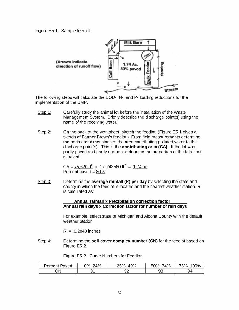
62
Figure E5-1. Sample feedlot.
The following steps will calculate the BOD-, N-, and P- loading reductions for the implementation of the BMP. Step 1: Carefully study the animal lot before the installation of the Waste
Management System. Briefly describe the discharge point(s) using the name of the receiving water.
Step 2: On the back of the worksheet, sketch the feedlot. (Figure E5-1 gives a
sketch of Farmer Brown’s feedlot.) From field measurements determine the perimeter dimensions of the area contributing polluted water to the discharge point(s). This is the contributing area (CA). If the lot was partly paved and partly earthen, determine the proportion of the total that is paved.
CA = 75,620 ft2 x 1 ac/43560 ft2 = 1.74 ac
Percent paved = 80% Step 3: Determine the average rainfall (R) per day by selecting the state and
county in which the feedlot is located and the nearest weather station. R is calculated as:
Annual rainfall x Precipitation correction factor_______ Annual rain days x Correction factor for number of rain days For example, select state of Michigan and Alcona County with the default weather station.
R = 0.2848 inches
Step 4: Determine the soil cover complex number (CN) for the feedlot based on Figure E5-2.
Figure E5-2. Curve Numbers for Feedlots
Percent Paved 0%–24% 25%–49% 50%–74% 75%–100% CN 91 92 93 94
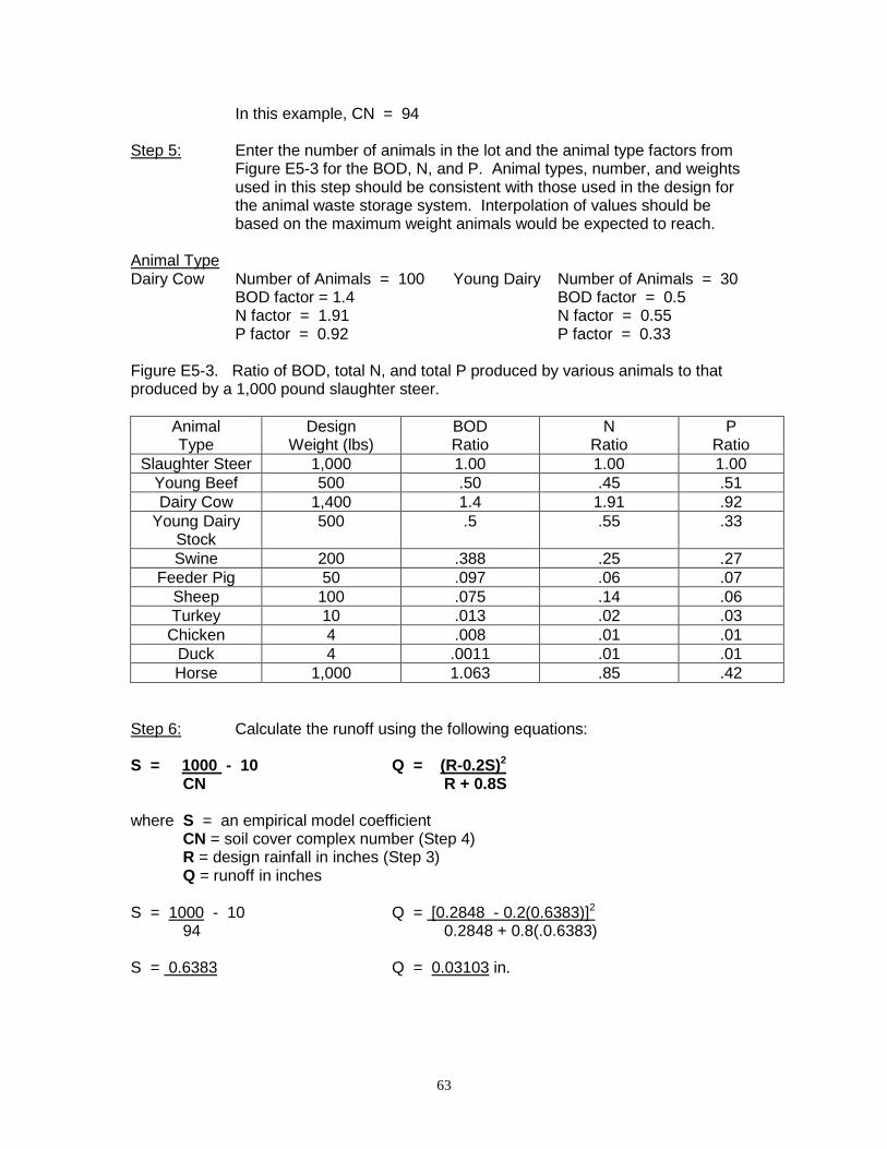
63
In this example, CN = 94 Step 5: Enter the number of animals in the lot and the animal type factors from
Figure E5-3 for the BOD, N, and P. Animal types, number, and weights used in this step should be consistent with those used in the design for the animal waste storage system. Interpolation of values should be based on the maximum weight animals would be expected to reach.
Animal Type Dairy Cow Number of Animals = 100 Young Dairy Number of Animals = 30 BOD factor = 1.4 BOD factor = 0.5 N factor = 1.91 N factor = 0.55
P factor = 0.92 P factor = 0.33 Figure E5-3. Ratio of BOD, total N, and total P produced by various animals to that produced by a 1,000 pound slaughter steer.
Animal Type
Design Weight (lbs)
BOD Ratio
N Ratio
P Ratio
Slaughter Steer 1,000 1.00 1.00 1.00 Young Beef 500 .50 .45 .51 Dairy Cow 1,400 1.4 1.91 .92
Young Dairy Stock
500 .5 .55 .33
Swine 200 .388 .25 .27 Feeder Pig 50 .097 .06 .07
Sheep 100 .075 .14 .06 Turkey 10 .013 .02 .03
Chicken 4 .008 .01 .01 Duck 4 .0011 .01 .01 Horse 1,000 1.063 .85 .42
Step 6: Calculate the runoff using the following equations: S = 1000 - 10 Q = (R-0.2S)2 CN R + 0.8S where S = an empirical model coefficient CN = soil cover complex number (Step 4) R = design rainfall in inches (Step 3) Q = runoff in inches S = 1000 - 10 Q = [0.2848 - 0.2(0.6383)]2
94 0.2848 + 0.8(.0.6383) S = 0.6383 Q = 0.03103 in.
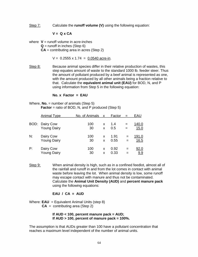
64
Step 7: Calculate the runoff volume (V) using the following equation: V = Q x CA where V = runoff volume in acre-inches Q = runoff in inches (Step 6) CA = contributing area in acres (Step 2) V = 0.2555 x 1.74 = 0.0540 acre-in. Step 8: Because animal species differ in their relative production of wastes, this step equates amount of waste to the standard 1000 lb. feeder steer. Thus the amount of pollutant produced by a beef animal is represented as one, with the amount produced by all other animals being a fraction relative to that. Calculate the equivalent animal unit (EAU) for BOD, N, and P
using information from Step 5 in the following equation: No. x Factor = EAU Where, No. = number of animals (Step 5) Factor = ratio of BOD, N, and P produced (Step 5) Animal Type No. of Animals x Factor = EAU BOD: Dairy Cow 100 x 1.4 = 140.0 Young Dairy 30 x 0.5 = 15.0 N: Dairy Cow 100 x 1.91 = 191.0 Young Dairy 30 x 0.55 = 16.5 P: Dairy Cow 100 x 0.92 = 92.0 Young Dairy 30 x 0.33 = 9.9 Step 9: When animal density is high, such as in a confined feedlot, almost all of the rainfall and runoff in and from the lot comes in contact with animal waste before leaving the lot. When animal density is low, some runoff may escape contact with manure and thus not be contaminated.
Calculate the Animal Unit Density (AUD) and percent manure pack using the following equations:
EAU / CA = AUD
Where: EAU = Equivalent Animal Units (step 8) CA = contributing area (Step 2) If AUD < 100, percent manure pack = AUD; If AUD > 100, percent of manure pack = 100%. The assumption is that AUDs greater than 100 have a pollutant concentration that reaches a maximum level independent of the number of animal units.
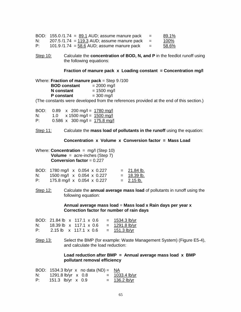
65
BOD: 155.0 /1.74 = 89.1 AUD; assume manure pack = 89.1% N: 207.5 /1.74 = 119.3 AUD; assume manure pack = 100% P: 101.9 /1.74 = 58.6 AUD; assume manure pack = 58.6% Step 10: Calculate the concentration of BOD, N, and P in the feedlot runoff using
the following equations: Fraction of manure pack x Loading constant = Concentration mg/l Where: Fraction of manure pack = Step 9 /100 BOD constant = 2000 mg/l N constant = 1500 mg/l
P constant = 300 mg/l (The constants were developed from the references provided at the end of this section.) BOD: 0.89 x 200 mg/l = 1780 mg/l N: 1.0 x 1500 mg/l = 1500 mg/l P: 0.586 x 300 mg/l = 175.8 mg/l Step 11: Calculate the mass load of pollutants in the runoff using the equation: Concentration x Volume x Conversion factor = Mass Load Where: Concentration = mg/l (Step 10) Volume = acre-inches (Step 7) Conversion factor = 0.227 BOD: 1780 mg/l x 0.054 x 0.227 = 21.84 lb. N: 1500 mg/l x 0.054 x 0.227 = 18.39 lb. P: 175.8 mg/l x 0.054 x 0.227 = 2.15 lb. Step 12: Calculate the annual average mass load of pollutants in runoff using the
following equation: Annual average mass load = Mass load x Rain days per year x
Correction factor for number of rain days BOD: 21.84 lb x 117.1 x 0.6 = 1534.3 lb/yr N: 18.39 lb x 117.1 x 0.6 = 1291.8 lb/yr
P: 2.15 lb x 117.1 x 0.6 = 151.3 lb/yr Step 13: Select the BMP (for example: Waste Management System) (Figure E5-4),
and calculate the load reduction: Load reduction after BMP = Annual average mass load x BMP
pollutant removal efficiency BOD: 1534.3 lb/yr x no data (ND) = NA N: 1291.8 lb/yr x 0.8 = 1033.4 lb/yr P: 151.3 lb/yr x 0.9 = 136.2 lb/yr
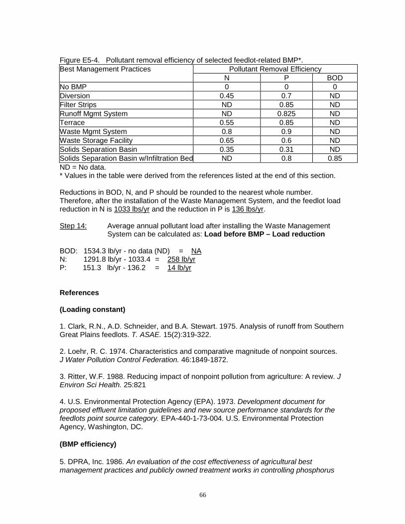
66
Figure E5-4. Pollutant removal efficiency of selected feedlot-related BMP*.
Pollutant Removal Efficiency Best Management Practices N P BOD No BMP 0 0 0 Diversion 0.45 0.7 ND Filter Strips ND 0.85 ND Runoff Mgmt System ND 0.825 ND Terrace 0.55 0.85 ND Waste Mgmt System 0.8 0.9 ND Waste Storage Facility 0.65 0.6 ND Solids Separation Basin 0.35 0.31 ND Solids Separation Basin w/Infiltration Bed ND 0.8 0.85 ND = No data. * Values in the table were derived from the references listed at the end of this section. Reductions in BOD, N, and P should be rounded to the nearest whole number. Therefore, after the installation of the Waste Management System, and the feedlot load reduction in N is 1033 lbs/yr and the reduction in P is 136 lbs/yr. Step 14: Average annual pollutant load after installing the Waste Management
System can be calculated as: Load before BMP – Load reduction BOD: 1534.3 lb/yr - no data (ND) = NA N: 1291.8 lb/yr - 1033.4 = 258 lb/yr P: 151.3 lb/yr - 136.2 = 14 lb/yr References (Loading constant) 1. Clark, R.N., A.D. Schneider, and B.A. Stewart. 1975. Analysis of runoff from Southern Great Plains feedlots. T. ASAE. 15(2):319-322. 2. Loehr, R. C. 1974. Characteristics and comparative magnitude of nonpoint sources. J Water Pollution Control Federation. 46:1849-1872. 3. Ritter, W.F. 1988. Reducing impact of nonpoint pollution from agriculture: A review. J Environ Sci Health. 25:821 4. U.S. Environmental Protection Agency (EPA). 1973. Development document for proposed effluent limitation guidelines and new source performance standards for the feedlots point source category. EPA-440-1-73-004. U.S. Environmental Protection Agency, Washington, DC. (BMP efficiency) 5. DPRA, Inc. 1986. An evaluation of the cost effectiveness of agricultural best management practices and publicly owned treatment works in controlling phosphorus
67
pollution in the Great Lakes basin. Prepared for U.S. Environmental Protection Agency, Washington, DC. 6. Edwards, W.M., L.B. Owens, and R.K. White. 1983. Managing runoff from a small, paved beef feedlot. J Environ Qual. 12(2). 7. Edwards, W.M., L.B. Owens, R.K. White, and N.R. Fausey. 1986. Managing feedlot runoff with a settling basin plus tiled infiltration bed. T ASAE. 29(1):243-247. 8. U.S. Environmental Protection Agency (EPA). 1993. Guidance specifying management measures for sources of nonpoint pollution in coastal waters. EPA-840-B-92-002. Office of Water, U.S. Environmental Protection Agency, Washington, DC. (STEPL) 9. Tetra Tech, Inc. 2002. User’s guide: Spreadsheet tool for the estimation of pollutant load (STEPL). Version 2.01. Prepared for U.S. Environmental Protection Agency, Washington, DC. (The current User's Guide is for STEPL version 3.1, 2005)

68
Exhibit 6 Algorithm through an Example: Urban Runoff Worksheet
Urban runoff can be attributed to many things, including the amount of rainfall, the soil conditions, and the degree of urbanization. Urban areas usually have high percentages of hard, impermeable surfaces. Fields and forests allow for the rainwater to soak into the soil where it falls, but parking lots, roofs, streets, and other impervious surfaces of an urban environment cause the rainwater to collect, and it must be forced out through a storm drain system. If the drainage system does not connect to a wastewater treatment facility, the rainwater and everything in it travels into local streams and rivers.
Urban runoff contributes many pollutants to the nearby streams and lakes. Some of these pollutants are nitrogen, phosphorus, sediment, lead, zinc, copper, cadmium, chromium, and arsenic. In addition to contributing pollutants, urbanization affects other water quality characteristics. These characteristics include water temperature, pH, dissolved oxygen, alkalinity, hardness, and conductivity.
Implementing best management practices (BMPs) in urban areas can reduce the pollutants carried by runoff to the nearby steams and lakes. The following example illustrates how to calculate pollutant load from a hypothetical urban area and the load reduction after implementing a BMP. Example: Determine the reduction in total nitrogen (TN) and total phosphorus (TP) loadings for an urban area (contributing/drainage area) after the implementation of vegetated filter strips. We use the Load Reduction Estimating Workbook (see Exhibit 5) to illustrate the calculation steps. The land use characteristics for the hypothetical area are as follows:
Land Use Area with storm water sewers (acres)
Area without storm water sewers (acres)
Commercial 50 0 Transportation 5 2
Step 1: Select a best management practice you want to implement in the
contributing/drainage area. Select the first option from the BMP list: Vegetated filter strips.
Step 2: Estimate the area in acres with and without storm water sewers for every
land use type in the contributing/drainage area. Commercial area with storm water sewers = 50 acres Transportation area with storm water sewers = 5 acres Transportation area without storm water sewers = 2 acres
Step 3: Calculate the load before BMP implementation for TN and TP in the
contributing/drainage area.
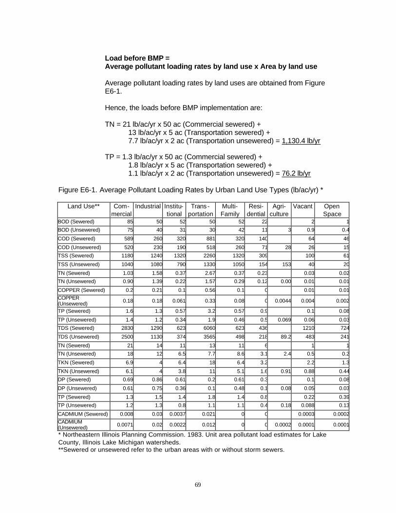
69
Load before BMP = Average pollutant loading rates by land use x Area by land use Average pollutant loading rates by land uses are obtained from Figure E6-1. Hence, the loads before BMP implementation are: TN = 21 lb/ac/yr x 50 ac (Commercial sewered) + 13 lb/ac/yr x 5 ac (Transportation sewered) + 7.7 lb/ac/yr x 2 ac (Transportation unsewered) = 1,130.4 lb/yr TP = 1.3 lb/ac/yr x 50 ac (Commercial sewered) + 1.8 lb/ac/yr x 5 ac (Transportation sewered) + 1.1 lb/ac/yr x 2 ac (Transportation unsewered) = 76.2 lb/yr
Figure E6-1. Average Pollutant Loading Rates by Urban Land Use Types (lb/ac/yr) *
Land Use**
Com-mercial
Industrial Institu-tional
Trans -portation
Multi-Family
Resi-dential
Agri-culture
Vacant Open Space
BOD (Sewered) 85 50 52 50 52 22 2 1
BOD (Unsewered) 75 40 31 30 42 11 3 0.9 0.4
COD (Sewered) 589 260 320 881 320 140 64 46
COD (Unsewered) 520 230 190 518 260 71 28 26 15
TSS (Sewered) 1180 1240 1320 2260 1320 309 100 61
TSS (Unsewered) 1040 1080 790 1330 1050 154 153 40 20
TN (Sewered) 1.03 1.58 0.37 2.67 0.37 0.23 0.03 0.02
TN (Unsewered) 0.90 1.39 0.22 1.57 0.29 0.12 0.00 0.01 0.01
COPPER (Sewered) 0.2 0.21 0.1 0.56 0.1 0 0.01 0.01COPPER (Unsewered) 0.18 0.18 0.061 0.33 0.08 0 0.0044 0.004 0.002
TP (Sewered) 1.6 1.3 0.57 3.2 0.57 0.9 0.1 0.08
TP (Unsewered) 1.4 1.2 0.34 1.9 0.46 0.5 0.069 0.06 0.03
TDS (Sewered) 2830 1290 623 6060 623 436 1210 724
TDS (Unsewered) 2500 1130 374 3565 498 218 89.2 483 241
TN (Sewered) 21 14 11 13 11 6 1 1
TN (Unsewered) 18 12 6.5 7.7 8.6 3.1 2.4 0.5 0.2
TKN (Sewered) 6.9 4 6.4 18 6.4 3.2 2.2 1.3
TKN (Unsewered) 6.1 4 3.8 11 5.1 1.6 0.91 0.88 0.44
DP (Sewered) 0.69 0.86 0.61 0.2 0.61 0.3 0.1 0.08
DP (Unsewered) 0.61 0.75 0.36 0.1 0.48 0.1 0.08 0.05 0.03
TP (Sewered) 1.3 1.5 1.4 1.8 1.4 0.8 0.22 0.39
TP (Unsewered) 1.2 1.3 0.8 1.1 1.1 0.4 0.18 0.088 0.13
CADMIUM (Sewered) 0.008 0.03 0.0037 0.021 0 0 0.0003 0.0002CADMIUM (Unsewered) 0.0071 0.02 0.0022 0.012 0 0 0.0002 0.0001 0.0001
* Northeastern Illinois Planning Commission. 1983. Unit area pollutant load estimates for Lake County, Illinois Lake Michigan watersheds. **Sewered or unsewered refer to the urban areas with or without storm sewers.

70
Step 4: Calculate the load after BMP implementation.
Load after BMP = Load before BMP x (1 - BMP pollutant removal efficiency)
BMP pollutant removal efficiencies (vegetated filter strips) for TN and TP pollutants are obtained from Figure E6-2. Hence, the loads after BMP implementation are: TN = 1130.4 lbs/yr x (1 - 0.4) = 678.24 lb/yr TP = 76.2 lbs/yr x (1 - 0.4525) = 41.7195 lb/yr
Figure E6-2. BMP Pollutant Removal Efficiencies (Maximum Efficiency = 1)
BMP Types Ref* BOD COD TSSLEAD COPPER ZINC TDS TN TKN DP TP CADMIUMVegetated Filter Strips A&B 0.505 0.4 0.73 0.45 U 0.6 U 0.4 U U 0.4525 U
Grass Swales A,B&C 0.3 0.25 0.65 0.7 0.5 0.6 U 0.1 U U 0.25 0.5
Infiltration Devises A 0.83 U 0.94 U U U U U U U 0.83 U
Extended Wet Detention A&B 0.72 U 0.86 0.4 U 0.2 U 0.55 U U 0.685 U
Wetland Detention A&B 0.63 0.5 0.78 0.65 U 0.35 U 0.2 U U 0.44 U
Dry Detention A&B 0.27 0.2 0.58 0.5 U 0.2 U 0.3 U U 0.26 U
Settling Basin A 0.56 U 0.82 U U U U U U U 0.515 U
Sand Filters A 0.4 U 0.83 U U U U U U U 0.375 U
WQ Inlets A&B 0.13 0.05 0.37 0.15 U 0.05 U 0.2 U U 0.09 U
Weekly Street Sweeping A 0.06 U 0.16 U U U U U U U 0.06 U
Infiltration Basin B&D U 0.65 0.75 0.65 U 0.65 U 0.6 U U 0.65 U
Infiltration Trench B&D U 0.65 0.75 0.65 U 0.65 U 0.55 U U 0.6 U
Porous Pavement B U 0.8 0.9 1 U 1 U 0.85 U U 0.65 U
Concrete Grid Pavement B U 0.9 0.9 0.9 U 0.9 U 0.9 U U 0.9 U
Sand Filter/Infiltration BasinB U 0.55 0.8 0.6 U 0.65 U 0.35 U U 0.5 U
WQ Inlet w/ Sand Filter B U 0.55 0.8 0.8 U 0.65 U 0.35 U U U U
Oil/Grit Separator B U 0.05 0.15 0.15 U 0.05 U 0.05 U U 0.05 U
Wet Pond B U 0.4 0.6 0.75 U 0.6 U 0.35 U U 0.45 U
Agriculture Filter Strip C U U U U U U U 0.5325 U U 0.6125 U U = Data unavailable * References: A Northeastern Illinois Planning Commission (NIPC). 1994. Model best management practice selection
methodology & Lake County decision-making framework. NIPC, Chicago, Illinois. B U.S. Environmental Protection Agency (EPA). 1993. Guidance specifying management measures for
sources of nonpoint pollution in coastal waters. EPA-840-B-92-002. Office of Water, Washington, DC. <http://www.epa.gov/OWOW/NPS/MMGI/Chapter4/index.html>.
C Leeds, R., L.C. Brown, M.R. Sulc, and L.VanLieshout. 1994. Vegetative filter strips: Application, installation and maintenance. AEX-467-94. Ohio State University Extension, Columbus, Ohio. <http://ohioline.osu.edu/aex-fact/0467.html>. Note: Took middle value of ranges for conflicting results
D Athayde, D.N., P.E. Shelly, E.D. Driscoll, D. Gaboury, and G. Boyd. 1983. Results of the nationwide urban runoff program. Volume I–final report. U.S. Environmental Protection Agency, Washington DC. 186 pages.
E Schueler, T.R. 1987. Controlling urban runoff: A practical manual for planning and designing urban BMPs. Metropolitan Washington Council of Governments, Washington, DC.

71
Step 5: Calculate the load reduction after the BMP implementation.
Load reduction = Load before BMP – Load after BMP TN Reduction: 1,130.4 – 678.24 = 452.16 lb/yr TP Reduction: 76.2 – 41.72 = 34.48 lb/yr