polymer solid state characterization - uni- · pdf filemsci polysci p104 – polymer solid...

MSci PolySci-Lab Modul P104

PPPooolllyyymmmeeerrrmmmaaattteeerrriiiaaallliiieeennn&&& PPPooolllyyymmmeeerrrttteeeccchhhnnnooolllooogggiiieee

Polymer Solid State Characterization

1 Introduction

Different methods are available for investigation and characterization of the solid state properties of polymeric materials. Besides different microscopic techniques such as REM, TEM, or POL, X-ray scattering is useful for the morphological characterization of semi-crystalline polymers to determine the degree of crystallinity and crystal modifications. In contrast, Differential Scanning Calorimetry (DSC) yields information about glass transition, melting, and crystallisation behaviour. Interesting for future applications are also optical properties and the density of materials. In this experiment isotactic polypropylene (i-PP) is characterized by several methods, such as WAXS, DSC, density, and optical parameters, to elucidate the influence of additives (nucleating and clarifying agents) on the polymer solid state and the end-use properties.

2 Literature

1. G. Strobl „The Physics of Polymers“, Springer-Verlag, Berlin Heidelberg 1996. 2. L.E. Alexander „X-Ray diffraction methods in Polymer Science“, Krieger 1979. 3. F.J. Baltà-Calleja „X-Ray Scattering of Synthetic Polymers“, Elsevier 1989. 4. I.M. Ward „Structure and Properties of Oriented Polymers“, Applied Science Publishers

1975. 5. J. Karger-Kocsis „Polypropylene, an A-Z Reference”, Kluwer Academic Publishers 1999. 6. Lecture "Polymermaterialien und Polymertechnologie", MSci PolySci, 7. Sem., Prof. H.-

W. Schmidt. (These references are not required reading material)

3 Prerequisite

For the lab experiment you need to be familiar with basics concepts of macromolecular science: Amorphous or semi-crystalline polymers; glass, melting, recrystallization temperature; polyolefines, melt flow index, tacticity (iso-, a-, and syndiotactic polymers), copolymers. The principles of a DSC measurement can be found on supplementary material on the web pages of modul P104.

MSci PolySci P104 – Polymer Solid State Characterization 2

4 Content

1 Introduction .......................................................................................................... 1 2 Literature .............................................................................................................. 1 3 Prerequisite .......................................................................................................... 1 4 Content ................................................................................................................ 2 5 Timing .................................................................................................................. 2 6 First Method: X-Ray Scattering of Polymers ........................................................ 3

6.1 Basic principles .......................................................................................................... 3 6.2 Generation of X-rays .................................................................................................. 4 6.3 Basics of scattering .................................................................................................... 5 6.4 Determination of polymer crystallinity by X-ray scattering ......................................... 7 6.5 Polymorphism in isotactic polypropylene ................................................................... 7 6.6 Experiment ................................................................................................................. 9

6.6.1 Safety information ............................................................................................................ 9 6.6.2 Assignments .................................................................................................................... 9

7 Second Method: Optical Properties of Polymers .................................................. 9 7.1 Basic principles .......................................................................................................... 9 7.2 Measurement of transparency ................................................................................. 10 7.3 Assignment .............................................................................................................. 11

8 Third Method: Differential Scanning Calometry (DSC) ....................................... 11 8.1 Basic Principles ........................................................................................................ 11 8.2 Nucleation ................................................................................................................ 12 8.3 Assignment .............................................................................................................. 13

9 Forth Method: Density measurements ............................................................... 13 9.1 Basic Principles ........................................................................................................ 13 9.2 Assignment .............................................................................................................. 14

5 Timing

Start with the WAXS experiment. During the measuring time of the WAXS, prepare the DSC samples and start the first run. In the meantime determine the optical properties and density of the polymer samples in FAN-A, back in NWII start the last DSC sample.


6 First Method: X-Ray Scattering of Polymers

Different methods are available for investigating the structure of multiphase polymeric materials. X-ray scattering is a very powerful technique for the morphological characterization of semi-crystalline polymers, microphase separated block copolymers, or polymer blends.

6.1 Basic principles Radiation can interact with matter in different ways. Radiation can be absorbed completely by excitation of nuclear, electronic, vibronic, or rotational states, which is the basic principle of spectroscopic methods such as NMR, Mössbauer-, UV-VIS- and IR-spectroscopy. In this case only energy transfer between radiation and matter occurs and the transitions between different energetic levels in the material contain information about its chemical components.

Radiation can also interact with matter without any energy loss and only the momentum of the radiation will be changed. In this case the radiation is diffracted or scattered. Although the first terminus is correct, often the second terminus is used in the literature. This so-called static scattering can be used to investigate the structure of a material by measuring the scattered intensity as a function of the angle.

Matter is not homogeneous in space from an atomistic point of view. These spatial fluctuations of density are the reason for scattering of radiation. Different kinds of fluctuations can be considered. In a single component system density fluctuations cause scattering (as in a gas or a liquid), while in mixtures of components the concentration fluctuations may lead to additional scattering. Concentration fluctuations lead to scattering only if the volume density of the scattering property is different for the different components.

To account only for concentration fluctuations, correction of the density fluctuations must be carried out. The question whether scattering can be observed or not is also a question of the length scale of the inhomogeneities as compared to the wavelength of the radiation.

There is also the possibility of partial energy transfer between radiation and matter combined with a scattering process. This happens for example when the scattering material is moving and the scattering process is superimposed by the Doppler-Effect. This so-called dynamic scattering gives information about velocities of the scattering structures in a sample. Diffusion coefficients or segmental motions within a polymer chain can be determined, depending on the time and length scales covered by the experiment.

X-rays interact with all the electrons of atoms, independent of their binding energy to the nucleus, because the energy of X-rays is usually much higher than the energy of electrons in an atom. The interaction between X-rays and electrons is rather weak and thus only a weak function of wavelength (if no absorption processes take place). The probability of interactions between radiation and matter depends on the density of these properties within the matter. For this reason in the case of X-rays, the number of electrons per unit-volume is an important quantity and atoms with a large order number contribute to X-ray scattering intensity more than atoms with smaller order numbers. Thus, the terminus electron density is often used.


The basic quantity important for X-ray scattering is the electron radius, which has the dimension of a length (scattering length). The density of the square of the scattering length is important for the scattering power (or scattering strength) of the system. The square of the scattering length is called cross section. The larger the cross section, the larger the probability is that a scattering process occurs when radiation passes through the sample. The cross sections of X-ray scattering is thus related to the density [g/cm3] of the material.

In a good scattering experiment most of the incident photons passing through the sample are transmitted, i.e. pass through the sample without any interactions. This can be achieved by using sufficiently thin samples. Otherwise a photon may interact more than one time with the sample, leading to multiple scattering. Multiple scattering is not useful for gaining structural information of the sample, since no unambiguous relation between the direction of the finally scattered (and detected) photon and the incident direction of the beam can be determined.

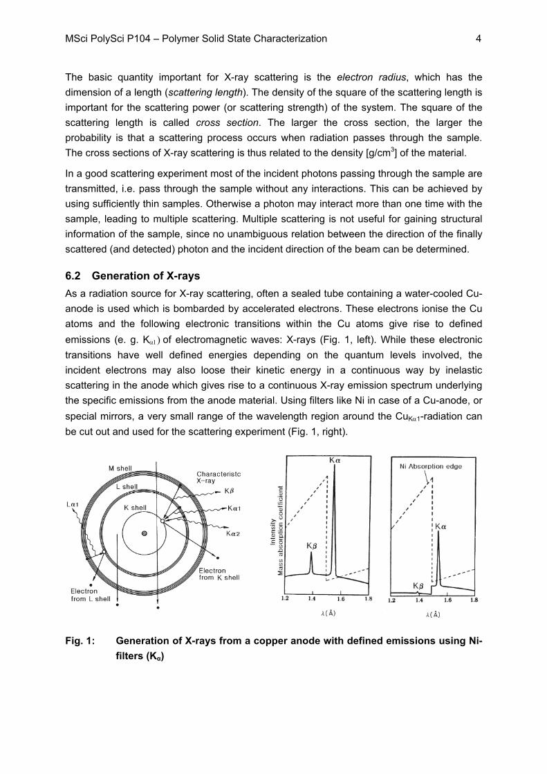
6.2 Generation of X-rays As a radiation source for X-ray scattering, often a sealed tube containing a water-cooled Cu-anode is used which is bombarded by accelerated electrons. These electrons ionise the Cu atoms and the following electronic transitions within the Cu atoms give rise to defined emissions (e. g. Kα1) of electromagnetic waves: X-rays (Fig. 1, left). While these electronic transitions have well defined energies depending on the quantum levels involved, the incident electrons may also loose their kinetic energy in a continuous way by inelastic scattering in the anode which gives rise to a continuous X-ray emission spectrum underlying the specific emissions from the anode material. Using filters like Ni in case of a Cu-anode, or special mirrors, a very small range of the wavelength region around the CuKα1-radiation can be cut out and used for the scattering experiment (Fig. 1, right).

Fig. 1: Generation of X-rays from a copper anode with defined emissions using Ni-filters (Kα)


6.3 Basics of scattering In the following scheme the set-up of a scattering experiment is shown schematically.

ki

kf q2θ2θ

X-ray source Detector

Sample

θ

Fig. 2 Experimental setup for a scattering experiment.

The radiation coming from the source is scattered by the sample, the detector registers the scattered rays. The glancing angle (Bragg angle) θ is defined as the angle between the scattered (diffracted) beam and the lattice plane. Hence, the angle between the scattered beam and the primary beam is 2θ. (Note that in the literature also often a scattering angle of θ is used; here the scattering angle is the double Bragg angle 2θ).

In the scheme also the wave vectors of the initial intensity ki, and the scattered intensity kf, as well as the scattering vector q are shown. They are connected by

if kkq −=

For elastic scattering (no energy transfer) the absolute magnitudes of both wave vectors are the same:

λπ

==2kk fi

Then for the absolute magnitude of the scattering vector follows

θλπqq sin4

==

Θ Θ

dhklλ2n

λ2n

Fig. 3 Scheme for derivation of Bragg’s law.


As can be seen from the equation above, a well defined wavelength is important in order to relate the scattering angle accurately to the scattering vector.

The periodic array of scattering centres will lead to a maximum at certain angles in the scattered intensity, as it can be seen from the above scheme. The scattering vectors corresponding to these maxima (i. e. where constructive interference of scattered waves is observed) can be related to the distance between the scattering centres:

Bragg’s law: n d hklλ θ= 2 sin

or, using the definition of the scattering vector Bragg’s law reads as

dn

qhkl =2π

n (integer) is the order of the diffraction, dhkl is the distance between net planes characterised by the Miller indices hkl. The Miller indices are integer numbers. The net plane is characterised by the points where it intersects the axes A, B and C of the basic crystal unit, a/h, b/k and c/l, respectively. a, b and c are the lengths of the basic vectors a, b and c.

According to Bragg’s law, the scattering angle (as expressed by q) is inversely related to the distance in the real space. That is why q characterises the reciprocal space. It becomes obvious that the wavelength of the radiation limits the values for dhkl towards small values. On the other hand, in principle with any wavelength even large distances should be detectable. However, the experimental problem to be solved in these cases is to separate scattered radiation at very low angles from the directly transmitted beam. Note that the fraction of scattered X-rays in comparison with the transmitted X-rays is in the order of 10-4. Therefore, in the case of large structures also larger wavelengths are used, in order to measure the desired length scale at angles well apart from the primary beam. Another possibility is to increase the distance between sample and detector. In consequence, scattered intensity is measurable even at small angles. Therefore, small angle scattering (SAXS) set-ups are usually larger as compared to wide angle scattering (WAXS) set-ups.

The scattered intensity I(q) can be expressed as the product of the structure factor (scattering factor) S(q) describing the spatial arrangements of the scattering centres and the contrast factor, K(q), expressing the scattering power of the material.

I(q) = K(q) S(q)

The contrast factor is a function of q, if the scattering units are of comparable size as the length scale under investigation. Studying atomic or molecular crystals with dimensions in the order of 1 nm require the knowledge of the shape of the involved atoms, or more precisely of their electronic structure. If larger length scales in the order of 10 to 100 nm are investigated, atoms are so small in comparison that they can be considered as structureless points. In that case, the contrast factor is no function of q. In polymers, often repeating units are taken as scattering units and their scattering power is calculated just from the number of electrons in a repeating unit divided by its volume.


10 15 20 25 30

0

20000

40000

60000

80000

100000

120000

Inte

nsity

[a.u

.]

2Θ [°]

crystalline part

amorphous part

In materials with crystal-like order, as in microphase separated block copolymers, the structure factor can be considered as a product of the form factor (of lamellae, cylinders or spheres) and the lattice factor describing their relative spatial arrangements. In dilute solutions, the structure factor consists only of the form factor of the dilute material (colloidal particles, macromolecular chain molecules etc.).

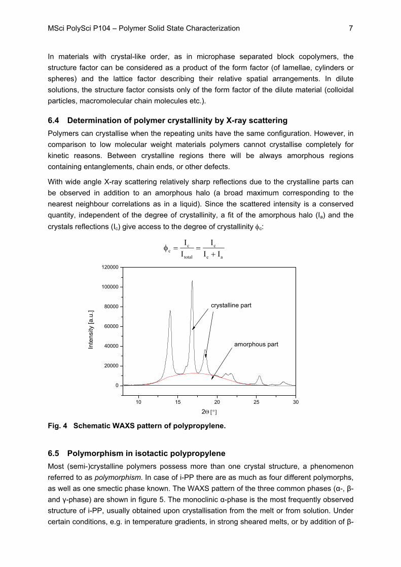
6.4 Determination of polymer crystallinity by X-ray scattering Polymers can crystallise when the repeating units have the same configuration. However, in comparison to low molecular weight materials polymers cannot crystallise completely for kinetic reasons. Between crystalline regions there will be always amorphous regions containing entanglements, chain ends, or other defects.

With wide angle X-ray scattering relatively sharp reflections due to the crystalline parts can be observed in addition to an amorphous halo (a broad maximum corresponding to the nearest neighbour correlations as in a liquid). Since the scattered intensity is a conserved quantity, independent of the degree of crystallinity, a fit of the amorphous halo (Ia) and the crystals reflections (Ic) give access to the degree of crystallinity φc:

ac

c

total

cc II

III

+==φ

Fig. 4 Schematic WAXS pattern of polypropylene.

6.5 Polymorphism in isotactic polypropylene Most (semi-)crystalline polymers possess more than one crystal structure, a phenomenon referred to as polymorphism. In case of i-PP there are as much as four different polymorphs, as well as one smectic phase known. The WAXS pattern of the three common phases (α-, β- and γ-phase) are shown in figure 5. The monoclinic α-phase is the most frequently observed structure of i-PP, usually obtained upon crystallisation from the melt or from solution. Under certain conditions, e.g. in temperature gradients, in strong sheared melts, or by addition of β-


nucleating agents, the formation of the hexagonal β-modification is predominant. The application of β-iPP is favoured in some fields, based on its high impact strength and toughness compared to α-iPP. The less common triclinic γ-phase is meta-stable and occurs only under high pressure and shear during crystallisation process and when stereochemical defects are introduced into the polymer backbones (copolymers). Upon mechanical deformation or thermal treatment, this modification transforms into the stable α-phase.

Fig. 5 WAXS patterns of the different polypropylene crystal modifications.

The ratio of the β-modification to the α-modification (β-content) is usually determined by WAXS measurements using methods of Turner-Jones. It is calculated directly from the ratio of height of main α-peaks (α1(110), α2(040) α3(130)) and the β-peak (β1(300)) with amorphous halo correction as shown in figure 6 and is called kb value.

)( 3211

1

αααββ

HHHHHkb +++

=

Fig. 6 WAXS pattern of polypropylene showing the main peaks for calculation of kb.


6.6 Experiment

6.6.1 Safety information Due to their energetic characteristics, X-rays are dangerous for biological materials. Note that X-rays for medical applications are generated by Tungsten anodes (W anodes), which have a much higher energy leading to much less absorption by the human body. In comparison to those X-rays, CuKα1-radiation is absorbed completely by the human body (mostly in the skin). The apparatus in use are completely shielded and equipped with safety circuits. Thus no radiation can penetrate the shields as long as they are operated in a proper way. Nothing may be touched by the participants of the lab course without clear instructions by the assistant.

6.6.2 Assignments WAXS measurements on four different polypropylene plaques will be performed:

- PP Basell Profax PH350

- PP Basell Profax PH350 additivated with the β-nucleating agent NJStar NU-100

- PP Basell Profax PH350 additivated with the clarifying agent Irgaclear XT386

- PP Borealis RF365MO (random copolymer; 2 wt% PE) additivated with Irgaclear XT386

Each group can choose which sample to measure, the scattering data of the other three samples will be provided by the assistants as file (please, bring along an USB data storage device). The measuring parameters you have to enter in the WAXS software are the scattering angle 2θ range (8° to 30°), the step size (0.025°) and the recording time at the respective angle (10 s). The assistants will help you to use the software and hardware of the X-ray apparatus. Note all parameters and PP grades. Determine the degree of crystallinity of the four PP samples according to the above mentioned procedure. Therefore plot the scattering intensity against the scattering angle 2θ for the four different samples, make a baseline correction, fit the amorphous halo and calculate the corresponding areas. Indentify the characteristic peaks of the different PP modifications and calculate the kb values. Compare and discuss all your results. Document the chemical structures of the nucleating/ clarifying agents.

7 Second Method: Optical Properties of Polymers

7.1 Basic principles Transparency and optical clarity are basic requirements for many commercial plastic products. Articles for medical use represent very good examples of such applications, where optical clarity is not only an aesthetical demand, but a necessary condition for the quick identification of the product. Polycarbonate (PC), Polymethylmethacrylat (PMMA) and amorphous polystyrene (PS) were used in such areas, since semi-crystalline polymers scatter light on the different units of their structure resulting in opaque products. In


polyolefins, the incident light is scattered on the crystallite spherulites and also on the interface between the amorphous and crystalline phases having different refractive indices. If the size of the crystalline unit is large enough to interfere with visible light, interference results in decreased transparency. The advantageous price/performance relations of poly-propylene (PP) and development both in processing as well as additive technology, led to a breakthrough for its use also in fields where optical clarity is demanded.

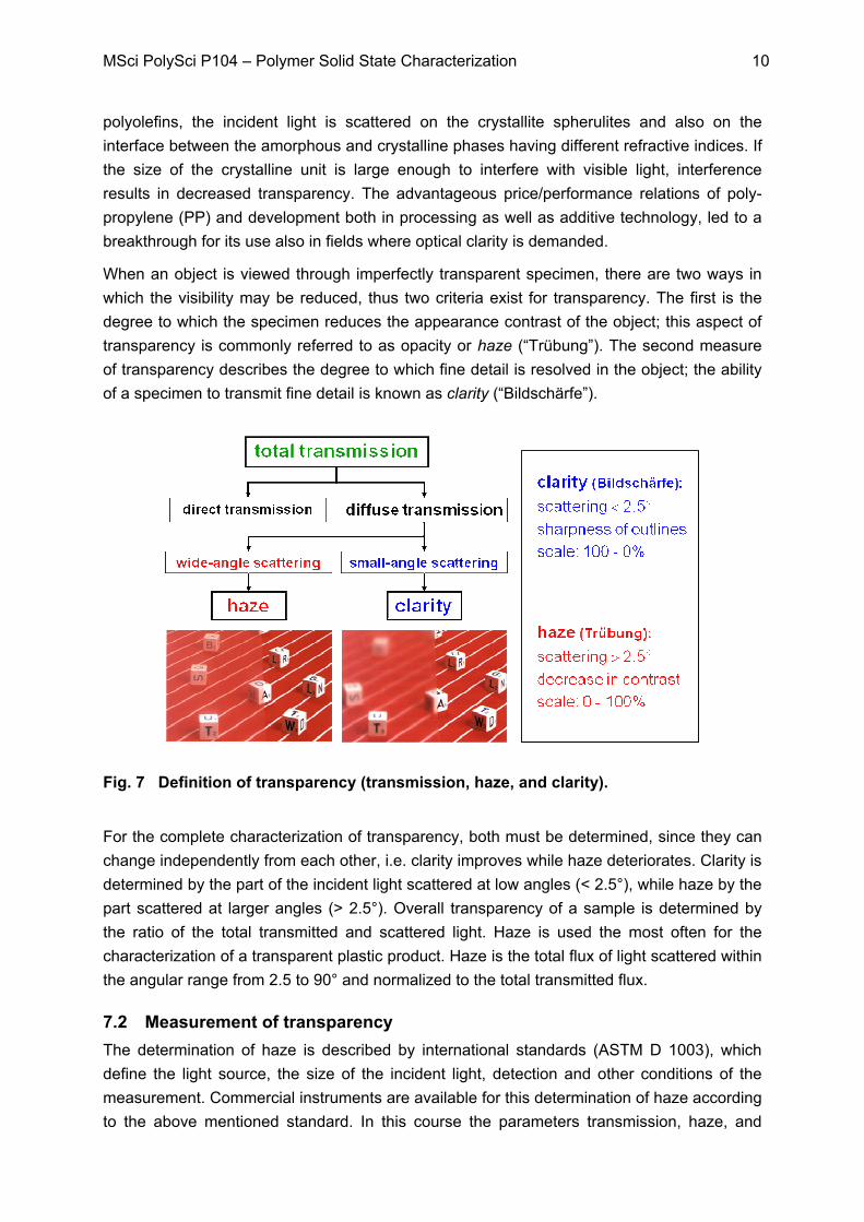
When an object is viewed through imperfectly transparent specimen, there are two ways in which the visibility may be reduced, thus two criteria exist for transparency. The first is the degree to which the specimen reduces the appearance contrast of the object; this aspect of transparency is commonly referred to as opacity or haze (“Trübung”). The second measure of transparency describes the degree to which fine detail is resolved in the object; the ability of a specimen to transmit fine detail is known as clarity (“Bildschärfe”).

Fig. 7 Definition of transparency (transmission, haze, and clarity).

For the complete characterization of transparency, both must be determined, since they can change independently from each other, i.e. clarity improves while haze deteriorates. Clarity is determined by the part of the incident light scattered at low angles (< 2.5°), while haze by the part scattered at larger angles (> 2.5°). Overall transparency of a sample is determined by the ratio of the total transmitted and scattered light. Haze is used the most often for the characterization of a transparent plastic product. Haze is the total flux of light scattered within the angular range from 2.5 to 90° and normalized to the total transmitted flux.

7.2 Measurement of transparency The determination of haze is described by international standards (ASTM D 1003), which define the light source, the size of the incident light, detection and other conditions of the measurement. Commercial instruments are available for this determination of haze according to the above mentioned standard. In this course the parameters transmission, haze, and


clarity will be measured with the haze-gard plus manufactured by BYC gardener. The following figure shows schematically the setup of the haze-gard plus. The apparatus has two ports, one for haze (large angle scattering) and one for clarity (small angle scattering). The incident light is focused on the sample and the transmitted/scattered light is detected in angles greater than 2.5° for the measurement of haze and smaller 2.5° as a measure for clarity.

Fig. 8 Experimental setup for measurements for optical properties

7.3 Assignment

Measure and document the optical properties (transmission, haze, and clarity) of the followings samples you produced in previous experiments:

- plaques of PP Borealis Borcom BG055AI (5 samples each with different thickness produced during the course Injection Molding)

- plaques of PP Borealis RF365MO with Irgaclear XT386 (5 samples each with different thickness produced during the course Injection Molding)

- films of PP Borealis RF365MO (2 samples with good surface quality and different film thickness produced during the course Extrusion)

Measure each sample thrice and use the mean value for your report. The assistants will help you to use the apparatus. Note all parameters (sample thickness) and PP grades. Compare and discuss all your results.

8 Third Method: Differential Scanning Calometry (DSC)

8.1 Basic Principles The basics and principles of the thermal analysis of polymers (differential scanning calometry; DSC) have already been covered in the “Bachelor Praktikum – Thermische Charakterisierung, Teil A”. For students who did not participate in that course, the lab handout can be found on the web pages of this module P104.


8.2 Nucleation As mentioned above, polymers do not crystallize completely due to their chain-like structure. There are only very few cases known, where polymers for a single crystal; these exceptions are not relevant for this lab. Thus they are of semi-crystalline nature (PE, PP) or amorphous like (PC, PMMA, a-PS). Supercooling, nucleation, and crystal growth are thereby crucial for the crystallization of polymer melts. During this process the polymer chains organise perpendicular to the crystallization plain and form lamellar structures that build up complex globular spherulites. The density and size of spherulites and thus important macroscopic properties (density, transparency, mechanical properties) are dependent on the supercooling of the polymer melt. During fast cooling many nucleus are being generated simultaneously yielding to small numerous spherulites. With slow cooling rates only few nucleus occur yielding to a small number of big spherulites. To enhance the crystallization, nucleating agents are often applied as additives in many technical relevant polymers. They are capable to increase the crystallization temperature and number of nucleus. Figure 9 shows two polarized optical micrographs of a neat (left) and additivated (right) polypropylene sample. One can easily notice the reduced spherulite size and higher density of nuclei due to additivation.

Fig. 9: Polarized optical micrographs of crystallized i-PP after cooling to room temperature; Left is neat polypropylene; Right is polypropylene with 0.15 wt% nucleating agent.

The nucleation efficiency (NE) is a measure for the performance of an additive reflecting the increase of the crystallization temperature. It is defined as

%TT

TT100NE

c1c2max

c1c

−−

=

where • Tc being the crystallization temperature of the additivated polymer • Tc1 being the crystallization temperature of the neat polymer under identical

conditions (reference value) • Tc2max being the maximum crystallization temperature that can be reached by self

nucleation (for iPP use Tc2max = 140,6 °C)


8.3 Assignment DSC measurements of granules of the following resins will be carried out:


- PP Basell Profax PH350 with Irgaclear XT386 Therefore 10-20 mg of the two grades will be weighted into aluminium pans, afterwards the following temperature scans will be performed:

• Heating from 130°C to 230°C with a heating rate of 10 K/min. The temperature will be held at 230°C for 5 minutes to ensure a complete melting of the crystalline fractions.

• Cooling from 230°C to 50°C with a cooling rate of 10 K/min to detect the first value for the crystallization temperature.

• Second heating scan to 230°C with 10 K/min and subsequent annealing for 5 minutes. Cooling under the same conditions to detect a second value for the crystallization temperature.

The assistants will help you using the DSC-software and –apparatus. The evaluation of the curves (slope correction, melting enthalpies) will be performed using the DSC-software. You will get the corrected data on USB stick, so plot the heat flow against the temperature for the two samples and assign the phase transition temperatures (Tm, Tc). Determine the nucleation efficiency of Irgaclear XT386 in iPP. Compare and discuss all your results. Determine the degree of crystallinity for both PP samples using the following equation:

0m

m

HH

α ∆=

∆

with mH∆ being the measured melting enthalpy and 0mH∆ being the theoretical melting

enthalpy of a hypothetic polypropylene (209 [J/g]) sample bearing a crystallinity of 100 %. Compare and discuss your results with the values obtained from your WAXS and density measurements.

9 Forth Method: Density measurements

9.1 Basic Principles Generally, the density of a body is defined as:

Vm

=ρ

By the determination of the mass (m) and volume (V) of a polymer sample, the density can be easily calculated. However density measurements of non-compact polymer specimens with unknown volume, such as for example polymer powders or pellets, may be difficult. Here, the density has to be determined using the Archimedean principle. For this method the


weight of the polymer will be determined under air and in a certain liquid. In this experiment, water at a defined temperature will be used. Then the buoyant force is given by VgF Lb ρ=

with ρL being the density of the liquid and g the gravitational acceleration. The net force of an immersed body is the sum of the buoyant force and the weight force: VgmgF Lnet ρ⋅=

From these equations one can easily calculate the density of the immersed sample.

LLmm

mρ

−=ρ

Considering the densities of the amorphous (ρa) and crystalline (ρc) regions, one can calculate the degree of crystallinity using the following equation:

ρρ−ρ

ρρ−ρ=α

)()(

ca

ca

9.2 Assignment

The density measurement will be carried out with a density balance which is located in the FAN-A. The following bulk samples will be weighted under air and in water.


- PP Basell Profax PH350 with NJStar NU-100

- PP Basell Profax PH350 with Irgaclear XT386

Calculate the density of all samples using the above derived equation. Determine also the degree of crystallinity with the literature values of the densities of the amorphous and crystalline parts (ρa = 0.854 g/cm3 and ρc = 0.931 g/cm3). Compare your results with the data received from the WAXS and DSC measurements.

polymer solid state characterization - uni- · pdf filemsci polysci p104 – polymer solid...

Documents