POLYNOMIAL TIME HEURISTIC OPTIMIZATION METHODS APPLIED TO PROBLEMS IN COMPUTATIONAL FINANCE

Ph.D. dissertation of

Fogarasi Norbert, M.Sc.

Supervisor:Dr. Levendovszky János, D. Sc.

Doctor of the Hungarian Academy of Sciences

Department of TelecommunicationsBudapest University of Technology and Economics

Budapest, 2014 May 20

1

Outline of Presentation

• Introduction

• Motivation: Computational Finance and NP hard probems

• My contributions

• Thesis Group I. Mean reverting portfolio selection

• Thesis Group II. Optimal scheduling on identical machines

• Summary of results and real world applications

2

Computational Finance and NP hard problems• Relatively new branch of computer science (Markowitz 1950s Modern

Portfolio Theory. Nobel Prize in 1990)• Numerical methods and algorithms with huge focus on applicability

(quantitative study of markets, arbitrage, options pricing, mortgage securitization)

• Recent focus: Algorithmic trading, quantitative investing, high frequency trading

• Post the 2008 financial crisis financial services industry has faced new challenges:• Regulatory pressure (timely reporting, transparency)• High-frequency trading (flash crashes)• Unprecedented attention on cost and efficiency

• Focus of interest: Finding quick (polynomial time) approximate solutions to difficult (exponential, NP hard) in order to pave the way towards a safer financial world

3

Computational Finance Open Issues

My Contribution Challenges

Real-time portfolio identification

Overnight Monte-Carlo risk calculation scheduling

Polynomial time approximation

using stochastic optimization

Polynomial time heuristic

scheduling algorithms4

NP hard problems which need fast suboptimal solutions!

My Contribution (cont’d)

• Finding polynomial time approx solutions to NP hard problems:• Mean Reverting Portfolio selection (Thesis Group I)• Task Scheduling on Identical machines (Thesis Group II)

• Show measurable improvement to existing approximate methods• Prove practical applicability in real world settings• Have very quick runtime characteristics for high frequency trading, timely

regulatory reporting and hardware cost savings

• 5 refereed journal publications, 1 conference presentation

1. Fogarasi, N., Levendovszky, J. (2012) A simplified approach to parameter estimation and selection of sparse, mean reverting portfolios. Periodica Polytechnica, 56/1, 21-28.

2. Fogarasi, N., Levendovszky, J. (2012) Improved parameter estimation and simple trading algorithm for sparse, mean-reverting portfolios. Annales Univ. Sci. Budapest., Sect. Comp., 37, 121-144.

3. Fogarasi, N., Tornai, K., & Levendovszky, J. (2012) A novel Hopfield neural network approach for minimizing total weighted tardiness of jobs scheduled on identical machines. Acta Univ. Sapientiae, Informatica, 4/1, 48-66.

4. Tornai, K., Fogarasi, N., & Levendovszky, J. (2013) Improvements to the Hopfield neural network solution to the total weighted tardiness scheduling problem. Periodica Polytechnica, 57/1, 1-8.

5. Fogarasi, N., Levendovszky, J. (2013) Sparse, mean reverting portfolio selection using simulated annealing. Algorithmic Finance, 2/3-4, 197-211.

6. Fogarasi, N., Levendovszky, J. (2012) Combinatorial methods for solving the generalized eigenvalue problem with cardinality constraint for mean reverting trading. 9th Joint Conf. on Math and Comp. Sci. February 2012 Siofok, Hungary

5

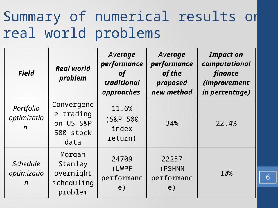
Summary of numerical results on real world problems

FieldReal world

problem

Average performance of traditional approaches

Average performance

of the proposed

new method

Impact on computational

finance (improvement in percentage)

Portfolio optimization

Convergence trading on US

S&P 500 stock data

11.6%(S&P 500

index return)34% 22.4%

Schedule optimization

Morgan Stanley

overnight scheduling

problem

24709 (LWPF performance)

22257 (PSHNN

performance)10%

6

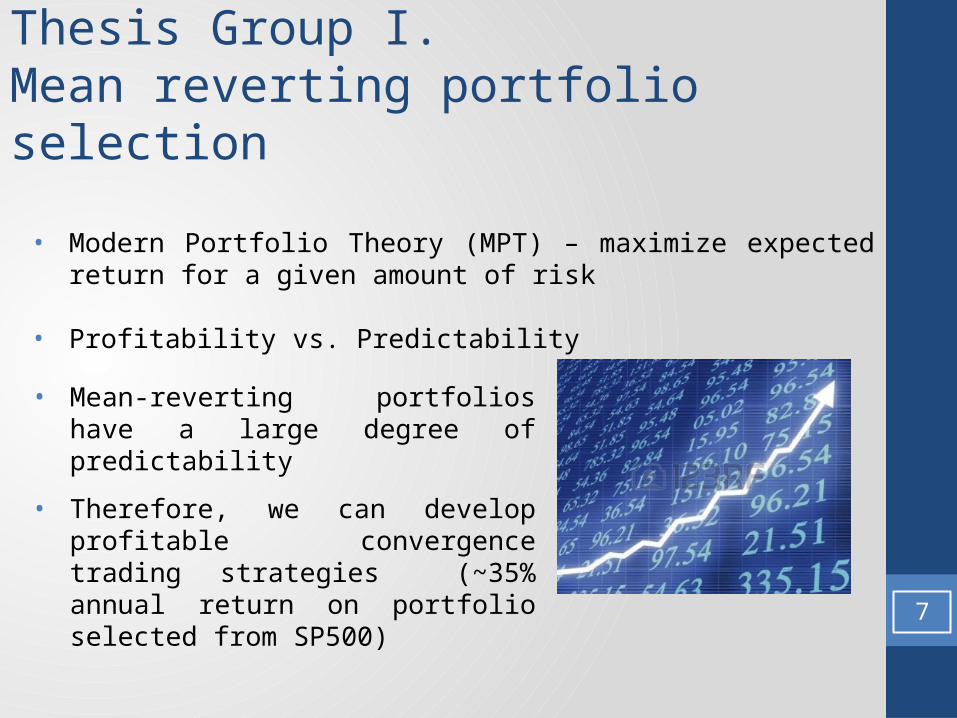
Thesis Group I. Mean reverting portfolio selection

• Modern Portfolio Theory (MPT) – maximize expected return for a given amount of risk

• Profitability vs. Predictability

• Mean-reverting portfolios have a large degree of predictability

• Therefore, we can develop profitable convergence trading strategies (~35% annual return on portfolio selected from SP500)

7

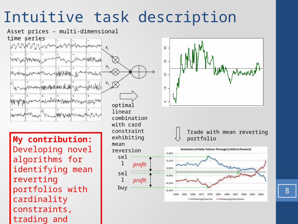
Intuitive task descriptionAsset prices – multi-dimensional time series

1x

2x

3x

optimal linear combination with card constraint exhibiting mean reversion

My contribution:Developing novel algorithms for identifying mean reverting portfolios with cardinality constraints, trading and performance analysis

Trade with mean reverting portfolio

profit

sellprofit

sell

buy8

Thesis Group I. Problem Description

How to identify mean reverting portfolios based on multivariate historical time series?

Constraint:

Sparse portfolio (limited transaction costs, easier to understand/interpret strategy)d’Aspremont, A.(2011) Identifying small mean-reverting

portfolios. Quantitative Finance, 11:3, 351-364

(Ecole Polytechnique, Paribas London, Phd-Stanford, Postdoc-Berkeley, Princeton)

9

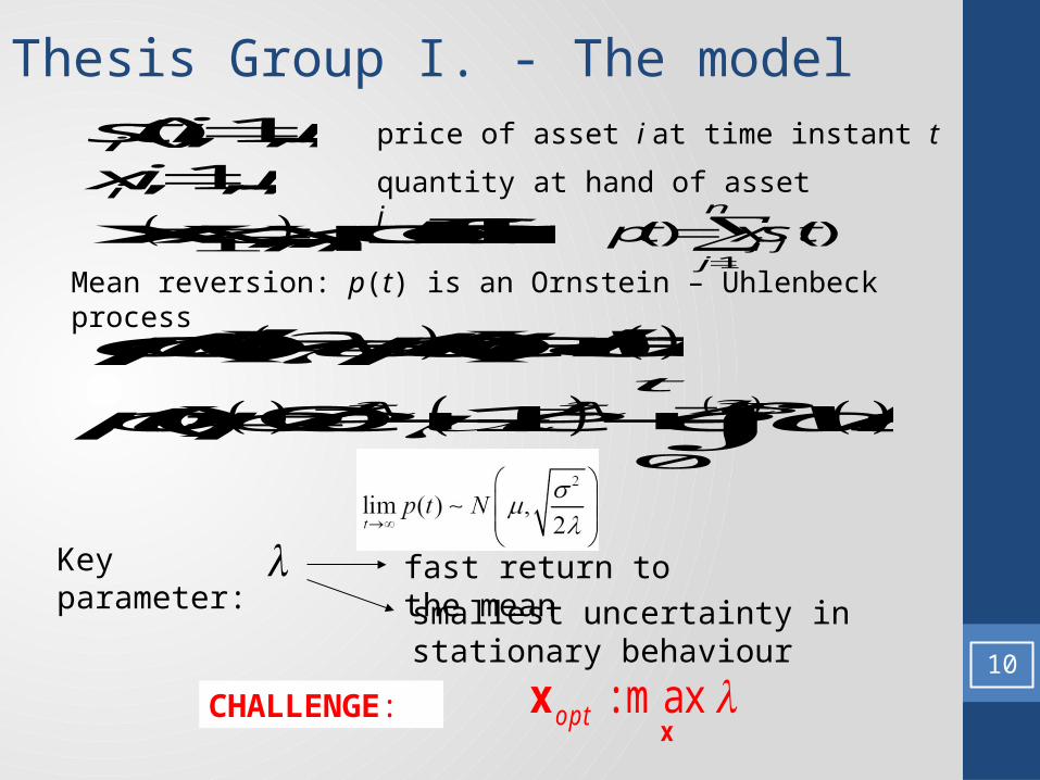
Thesis Group I. - The model

( ) ( )dp t p t dt dW t

Mean reversion: p(t) is an Ornstein – Uhlenbeck process

0

( ) 0 1t

t st tp t p e e e dW s

Key parameter:

fast return to the mean

smallest uncertainty in stationary behaviour

( ), 1,...,is t i n price of asset i at time instant t

, 1,...,ix i n quantity at hand of asset i

1

( ) ( )n

j jj

p t x s t

1,..., portfolio vectornx xx

CHALLENGE: : m axop t x

x10

The discrete model - VAR(1)First degree vector autoregressive process

11

1t t t s As w Tt tEG s s ,t Nw 0 Kwhere

1T T Tt t t s x s Ax w x

1 1:

T T T T Tt t

TT Tt t

E

E

x A s s Ax x A GAxx

x Gxx s s x

1 1: max max max

T T T T Tt t

opt TT Tt t

E

E

x x x

x A s s Ax x A GAxx x

x Gxx s s x  

 ~

 

Optimal portfolio as a generalized eigenvalue problem

1 1: max max max

T T T T Tt t

opt TT Tt t

E

E

x x x

x A s s Ax x A GAxx x

x Gxx s s x

under the constraints of 1; sparsecard k x x

; max. eigenvalueT A GAx Gx

det 0 max. rootT A GAx G

Problem: develop a fast solution to the generalized eigenvalue problem under the cardinality constraint – NP hard Poly time ?? 12

  

Thesis I.1 Estimation of Model Parameters

• Given nxT historical VAR(1) data st we need to estimate A, K (covar

matrix of W) and G (covar matrix of st)

• A and K can be estimated using max likelihood

• G can be estimated using sample covariance. Classical research focuses on regularization techniques (Dempster 1972, Banerjee et al 2008, d’Aspremont et al 2008, Rothman et al 2008)

1t t t s As W

2

11

ˆ : minT

t tt

A

A s As

11

1ˆ : ,1

TT

t ttT

G s s s s

13

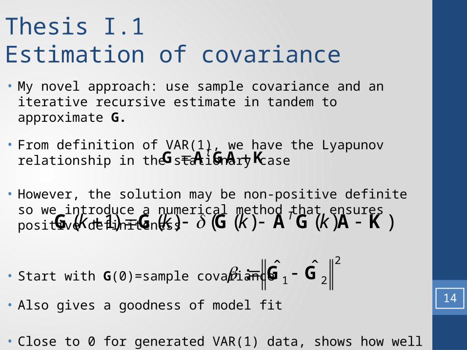
Thesis I.1 Estimation of covariance• My novel approach: use sample covariance and an iterative recursive

estimate in tandem to approximate G.

• From definition of VAR(1), we have the Lyapunov relationship in the stationary case

• However, the solution may be non-positive definite so we introduce a numerical method that ensures positive definiteness

• Start with G(0)=sample covariance

• Also gives a goodness of model fit

• Close to 0 for generated VAR(1) data, shows how well VAR(1) assumption works for real data.

T G A GA K

( 1) ( ) ( ( ) ( ) )Tk k k k G G G A G A K

2

1 2ˆ ˆ: G G

14

Thesis I.1 Numerical results

vs. t for n=8, σ=0.1, 0.3, 0.5, generating 100 independent time series for each t and plotting the average norm of error

0 200 400 600 800 1000 1200 1400 1600 1800 20000

0.05

0.1

0.15

0.2

0.25

0.3

0.35

0.4

0.45

0.5

2

1 2ˆ ˆG G

15

Cardinality reduction by exhaustive search

New selection, by visiting all the states fulfilling the cardinality constraints

Eigenvalue solver in the small space satisfying the cardinality constraint

: maxT T

opt Tx

x AGA xx

x Gx

: maxT T

opt Tx

x AGA xx

x Gx, ,

NxN KxK

A G A G

complexity, is there any better solution?!

!( )!

NO

K N K

Solution with the required cardinality (sparse portfolio)

Asset selection by dimension reduction (only a few assets)

Big space Small space

16

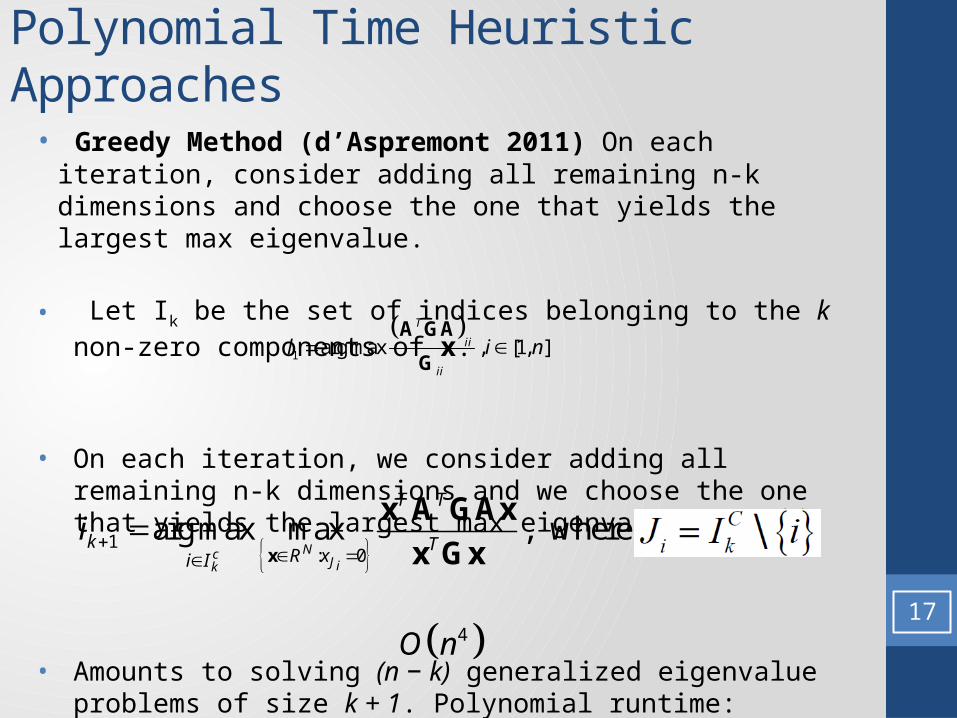
Polynomial Time Heuristic Approaches

• Greedy Method (d’Aspremont 2011) On each iteration, consider adding all remaining n-k dimensions and choose the one that yields the largest max eigenvalue.

• Let Ik be the set of indices belonging to the k non-zero components of x.

• On each iteration, we consider adding all remaining n-k dimensions and we choose the one that yields the largest max eigenvalue.

• Amounts to solving (n − k) generalized eigenvalue problems of size k + 1. Polynomial runtime:

17

1 arg max , [1, ]

T

ii

ii

l i n A GA

G

1

: 0arg max max , where

NcJik

T Tc

k i kTR xi I

i J I i

x

x A GAx

x Gx

4O n

Polynomial Time Heuristic Approaches

• Truncation Method (Fogarasi et al 2012) Compute unconstrained solution then use k heaviest dimensions to solve the constrained problem. Super fast heuristic (only 2 eigenvalue computations)

10 20 30 40 50 60 70 80 90 1000

5

10

15

20

25

30

35

Cardinality

CP

U R

untim

e (s

ec)

Greedy

Truncation

18

• Restrict the portfolio vector x to have only integer values of which only k are non-zero.

• Consider the Energy function to be minimized:

• At each step of the algorithm, we consider a neighboring state w' of the current state w and decide between moving or staying

• At each step, a random projection of the vector is performed to an appropriate subspace

T T

TE

w AGA ww

w Gw

( ') ( )1

1 if E( ) ( ')'

if E( ) ( ') n

n

E EnT

n

EP

e E

w w

w ww w

w w

Thesis I.2: Novel approach -Application of SA by random projection

19

• Cardinality constraint can easily be built into the neighbor function

• Starting point can be selected as Greedy solution

• Memory feature can be built in to ensure solution is at least as good as starting point

• Periodic revert to starting point improves performance

• Cooling schedule can be set to be fast enough for the specific application

• Procedure can be stopped at any point or an adaptive stopping condition has been developed.

Thesis I.2: Novel approach -Application of SA by random projection

20

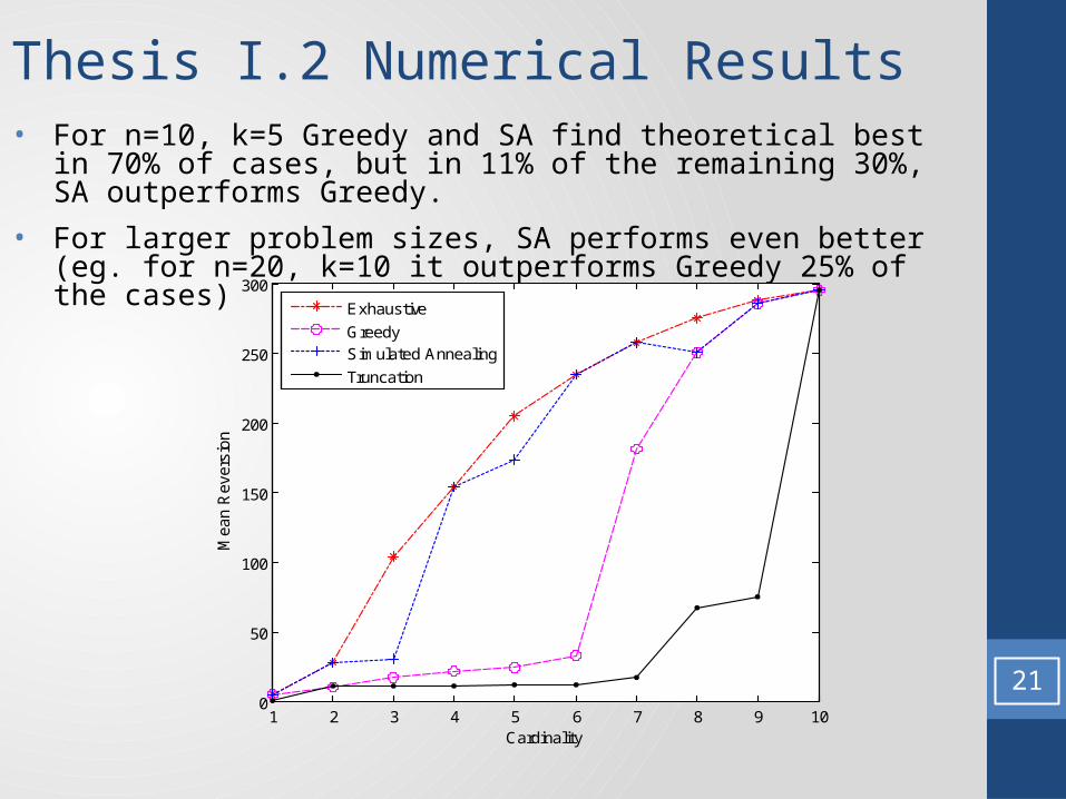
Thesis I.2 Numerical Results• For n=10, k=5 Greedy and SA find theoretical best in 70% of cases,

but in 11% of the remaining 30%, SA outperforms Greedy.

• For larger problem sizes, SA performs even better (eg. for n=20, k=10 it outperforms Greedy 25% of the cases)

1 2 3 4 5 6 7 8 9 100

50

100

150

200

250

300

Cardinality

Mea

n R

evers

ion

Exhaustive

GreedySimulated Annealing

Truncation

21

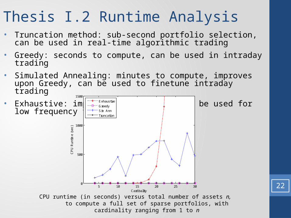
Thesis I.2 Runtime Analysis• Truncation method: sub-second portfolio selection, can be used in real-

time algorithmic trading

• Greedy: seconds to compute, can be used in intraday trading

• Simulated Annealing: minutes to compute, improves upon Greedy, can be used to finetune intraday trading

• Exhaustive: impractical for n>20, can be used for low frequency trading

5 10 15 20 25 300

500

1000

1500

Cardinality

CP

U R

untim

e (s

ec)

Exhaustive

GreedySim Ann

Truncation

CPU runtime (in seconds) versus total number of assets n, to compute a full set of sparse portfolios, with cardinality ranging from 1 to n

22

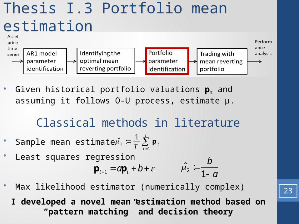
Thesis I.3 Portfolio mean estimation

• Given historical portfolio valuations pt and assuming it follows O-U process, estimate μ.

Classical methods in literature

• Sample mean estimate

• Least squares regression

• Max likelihood estimator (numerically complex)

I developed a novel mean estimation method based on “pattern matching” and decision theory

11

1ˆ :

T

ttT

p

1t ta b p p 2ˆ :1

b

a

23

Thesis I.3 Novel portfolio parameter estimation using pattern matching• Starting from definition of Ornstein-Uhlenbeck process:

• Taking expected value of the above:

• Use max likelihood estimation techniques to decide which pattern they match the most, and determine long term μ

where U is the time correlation matrix of pt

• This estimate is more accurate than sample mean and more resilient to small λ than linear regression.

( ) ( )dp t p t dt dW t

( ) (0) tt e

0

( ) 0 1t

t st tp t p e e e dW s

24

1

,1 1

31

,1 1

0 2 2 1

ˆ : .2 1

t ti j i j i

ji ji j

t ti j i j

i ji j

e e e e

e e e

U p

U

Thesis I.4 Simple Convergence Trading Model

• We are deciding whether μ(t)< μ by only observing p(t) using an approach based on decision theory

• We can use this simplified model to prove the economic viability of our algorithms and compare them to each other.

25

Observed sampleAccepted

hypothesisError probability

Action(Cash / Portfolio)

Buy / Hold

No Action / Sell

No Action / Sell

Thus the trading strategy can then be summarized as follows

As a result, for a given rate of acceptable error ε , we can select an α for which

Thesis I.4 Simple Convergence Trading Model

it can be said that we accept the stationary hypothesis which holds with probability

If process is in stationary state then the samples are generated by a Gaussian distribution

( )p t ( ), 1,...,p t t T2

,2

N

2

2

( )

/

2

11

2 / 2

u

e du

( ) ,p t

1 .

. As such, having observed the sample

26( )p t ( )t 2

2

( )

/

2

1/ 2

2 / 2

u

e du

( ) ,p t ( )t 2

2

( )

/

2

11

2 / 2

u

e du

( )p t ( )t 2

2

( )

/

2

1/ 2

2 / 2

u

e du

L=3 Greedy L=3 Sim Ann L=4 Greedy L=4 Sim Ann

75.00%

85.00%

95.00%

105.00%

115.00%

125.00%

135.00%

145.00%

155.00%SP500 Convergence Trading results

G_min

G_max

G_avg

G_final

• Consider the 500 stocks that make up the SP500 during 2009-2010 and select the K=4 stock portfolio to maximize mean-reversion.

• Repeat for 250 trading days (1 year)

• SP500 went up by 11.6%, our method generates 34% return

• Minimum, maximum, average and final portfolio values starting from 100%.

Thesis Group I. S&P500 Test

27

Thesis Group I. Summary

Thesis I.1New numerical method for estimating covariance matrix of VAR1 process

Periodica Polytechnica 2011

Thesis I.2Adopted simulated annealing to probl of maximizing mean reversion under cardinality constraint

Algorithmic Finance 2013

Thesis I.3Novel mean estimation technique for O-U processes using pattern matching

Annales Univ Sci Bp 2012

Thesis I.4Simple trading strategy based on decision theoretic formulation

Joint Conf on Math and Comp Sci 2012

28

• Complex portfolios are evaluated and risk managed using Monte-Carlo simulations at many financial institutions (eg. Morgan Stanley)

• Future trajectories of market variables are simulated and portfolio value/risk is evaluated on each trajectory, then a weighted avg is used

• Each night a changed portfolio needs to be evaluated/risk managed with new market data/model parameters

• Need a quick way to schedule 10000’s of jobs on 10000’s of machines in a near optimal way

• Why? $10M/year spend on hardware, timely response to clients and regulators regarding portfolio values and VaR.

• My novel method saved 53 minutes on top priority jobs running for 12 hours overnight, compared to the next best heuristic. 29

Thesis Group II. Optimal Scheduling

Time Steps

Thesis Group II. Problem Formulation

• Scheduling jobs on a finite number (V) of identical processors under constraints on the completion times

• Given n users/jobs of sizes

• Cutoff times

• Weights/priorities

• Scheduling matrix:

• Where if job i is processed at time step j.

• Jobs can stop/restart on different machine (preemption)

• For example V=2, n=3, x={2,3,1}, K={3,3,3}.

1 2, ,..., nnx x x x N

1 2, ,..., nnK K K K N

1 2, ,..., nnw w w w R

0,1n mC

, 1i j C

1 0 1

1 1 1

0 1 0

C 30Jobs

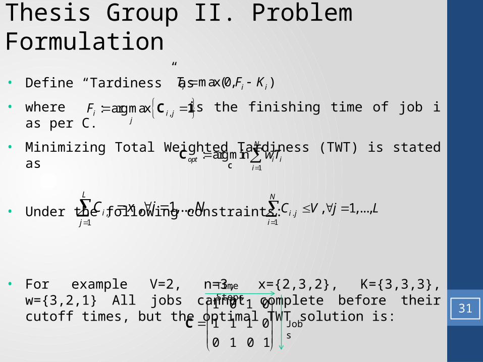
• Define “Tardiness” as

• where is the finishing time of job i as per C.

• Minimizing Total Weighted Tardiness (TWT) is stated as

• Under the following constraints:

• For example V=2, n=3, x={2,3,2}, K={3,3,3}, w={3,2,1} All jobs cannot complete before their cutoff times, but the optimal TWT solution is:

max(0, )i i iT F K

,: arg max 1i i jj

F C

1

: arg minN

opt i ii

wT

C

C

,1

, 1,...,L

i j ij

C i Nx

.1

, 1,...,i

N

ijC V j L

1 0 1 0

1 1 1 0

0 1 0 1

C

Thesis Group II. Problem Formulation

31

Time Steps

Jobs

Heuristic Approaches to TWT

• 1990 Du and Leung prove that TWT is NP-hard

• 1979 Dogramaci, Sulkis – simple heuristic

• 1983 Rachamadugu – myopic heuristic, compares to Earliest Due Date (EDD) and WSPT (Weighted Shortest Processing Time)

• 1998 Azizoglu – branch and bound heuristic, too slow > 15 jobs

• 1994 Koulamas – KPM algorithm

• 2000 Armentano – tabu search

• 1995 Guinet – simulated annealing, lower bound

• 2002 Sen, 2008 Biskup – Surveys of existing methods

• 2000 – Artificial Neural Network approach to scheduling problems

• 2004 Maheswaran – Hopfield Neural Network approach to single machine TWT on a specific 10-job problem.

32

• HNN are a recursive Neural Network which are good for solving quadratic optimization problems in the form

• Our task is to transform the TWT to a quadratic optimization problem.

1,

2T Tf y Wy b yy

1,

1

mini

LN

i i jj Ki

w C

, ,1 1

2

1

: minL L

i j i i j ij

N

ji

i C x C x

C

,1 1

2

.1

: minN N

i j

L

i ji i j

j C V C V

Thesis II.1 Novel Approach: TWT to QP

33

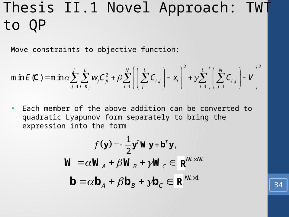
Move constraints to objective function:

• Each member of the above addition can be converted to quadratic Lyapunov form separately to bring the expression into the form

, ,

2 2

2

1 1 111

min ( ) minj

J L L N

i j i

N L

j jlij K i

i jl j j

E C x CC Vw

C

1,

2T Tf y Wy b yy

AN NL

CL

B WW WW 1

BN

A CL b bb b

Thesis II.1 Novel Approach: TWT to QP

34

R

R

Thesis II.1 Novel Approach: TWT to QP

Results of the matrix conversions:

1,A JLb 01

22A

J

D 0 0

W 0 D 0

0 0 D

*

j j j j

j j j j

K K K L K L Lj

L K K j L K L Kw

0 0D

0 I

1 1 11 22

L L LB Jx x x

b 2

L L

L LB

L L

1 0 0

0 1 0W

0 0 1

1 1 1 1 1 1, , , , , , ,C M L M M L M M L M b 0 V 0 V 0V

2C

D D D

D D DW

D D D

35

R

M M M L M

L M M L M L M

I 0

0D

0

Thesis II.2 Applying HNN

• Hopfield (1982) proved that the recursion

• converges to its fixed point, so minimizes a quadratic Lyapunov function

• I implemented this in MATLAB, including systematic selection of the heuristic constants α,β and γ. I also developed algorithms to validate and correct the resulting schedule matrix if needed.

1

ˆ( 1) sgn ( ) ,ˆ , modN

i ij j i Nj

k y k b i kW

y

1 1 1

1 1ˆˆ ˆ ˆ( ) : .2 2

N N NT T

ij i j i ii j i

W y y y b

y y Wy b yL

36

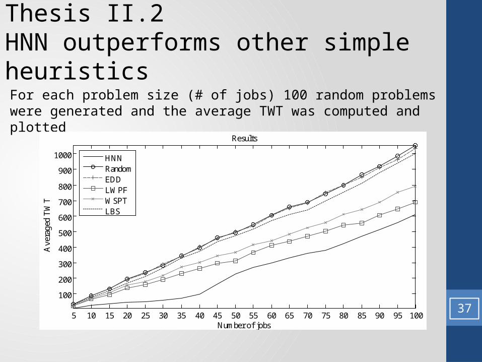
Thesis II.2 HNN outperforms other simple heuristics

For each problem size (# of jobs) 100 random problems were generated and the average TWT was computed and plotted

5 10 15 20 25 30 35 40 45 50 55 60 65 70 75 80 85 90 95 100

100

200

300

400

500

600

700

800

900

1000

Results

Number of jobs

Ave

rage

d T

WT

HNNRandomEDDLWPFWSPTLBS

37

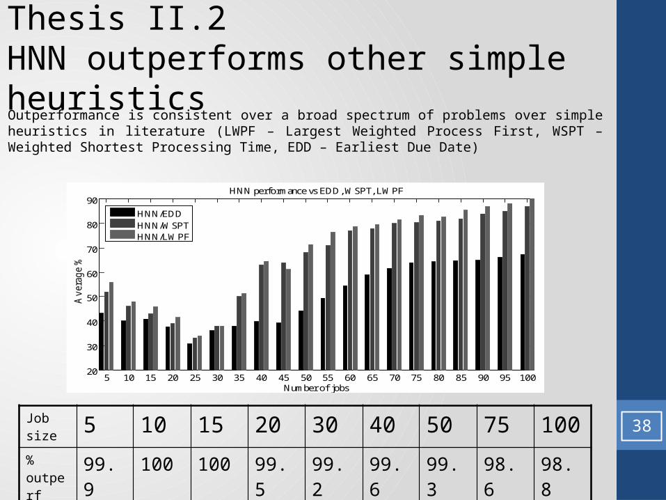
Thesis II.2 HNN outperforms other simple heuristicsOutperformance is consistent over a broad spectrum of problems over simple heuristics in literature (LWPF – Largest Weighted Process First, WSPT – Weighted Shortest Processing Time, EDD – Earliest Due Date)

Job size 5 10 15 20 30 40 50 75 100% outperf

99.9 100 100 99.5 99.2 99.6 99.3 98.6 98.8

5 10 15 20 25 30 35 40 45 50 55 60 65 70 75 80 85 90 95 10020

30

40

50

60

70

80

90HNN performance vs EDD, WSPT, LWPF

Number of jobs

Av

era

ge %

HNN/EDDHNN/WSPTHNN/LWPF

38

Thesis II.3 Further improving HNN

Smart HNN (SHNN)

• Use the result of Largest Weighted Path First (LWPF) as starting point for HNN rather than random starting points

• Speeds up HNN due to single starting point, but still require multiple iterations due to setting of heuristic constants.

Perturbed Smart HNN (PSHNN)

• Consider random perturbations of LWPF as starting point to HNN, in order to avoid getting stuck in local minima

39

Thesis II.3 Further improving HNN

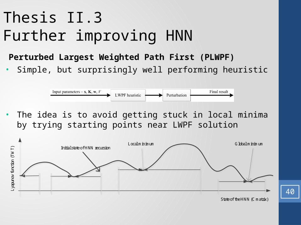
Perturbed Largest Weighted Path First (PLWPF)

• Simple, but surprisingly well performing heuristic

• The idea is to avoid getting stuck in local minima by trying starting points near LWPF solution

State of the HNN (C matrix)

Lya

puno

v fu

nctio

n (T

WT

) Initial state of HNN recursionLocal minimum Global minimum

40

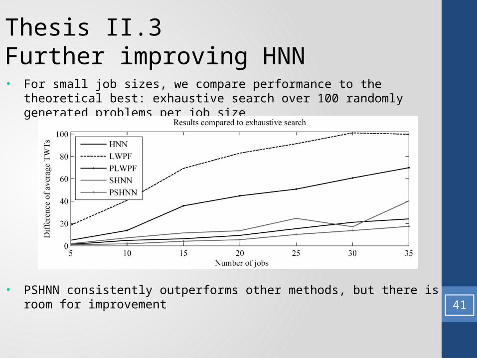
Thesis II.3 Further improving HNN• For small job sizes, we compare performance to the theoretical best:

exhaustive search over 100 randomly generated problems per job size

• PSHNN consistently outperforms other methods, but there is room for improvement 41

• PSHNN outperforms other methods by increasing margin as job size grows

Thesis II.3 Further improving HNN• For small job sizes, we compare performance to the theoretical best:

exhaustive search over 100 randomly generated problems per job size

42

Thesis Group II. Practical Application

• Monte Carlo simulation based risk calculations scheduling at Morgan Stanley overnight for trading and regulatory reporting

• 100 portfolios, 556 jobs, 792 seconds average size

• 7% improvement over HNN, 10% over LWPF (best method in literature prior to my study).

• 53 minutes saved on top 3 priority jobs compated to next best heuristic

Weight 3 4 5 6 7 8 9 10 SUM Increment to PSHNN

PSHNN 4401 11116 4020 1620 1092 8 0 0 22257 0%

PLWPF 3513 9624 5130 1788 490 312 2304 190 24019 5%

HNN 4404 11040 4735 1824 1092 456 468 0 24019 7%

LWPF 4404 11140 5470 2472 1183 40 0 0 24709 10%

EDD 4401 9940 1770 636 1134 464 22752 1430 42527 48%43

Thesis II.1 Thesis II.2 Thesis II.3I converted TWT problem to quadratic form including the constraints with heuristic constants

I applied the Hopfield Neural Net (HNN) and found approximate solutions in polynomial time

I showed that HNN solution outperforms other simple heuristics on large set of random problems

I improved HNN by intelligent selection of starting point and random perturbations

Acta Univ Sapientiae 2012

Acta Univ Sapientiae 2012 Periodica Polytechnica 2013

44

Thesis Group II. Optimal Scheduling

Numerical results on real world problems

FieldReal world

problem

Average performance of traditional approaches

Average performance

of the proposed

new method

Impact on computational

finance (improvement in percentage)

Portfolio optimization

Convergence trading on US

S&P 500 stock data

11.6%(S&P 500

index return)34% 22.4%

Schedule optimization

Morgan Stanley

overnight scheduling

problem

24709 (LWPF performance)

22257 (PSHNN

performance)10%

45

Managed to find a generic approach to approximating

NP hard problems in polynomial time using

heuristic methods

Proved the practical effectiveness and

applicability on real world problems for 2 very difficult

open problems Provides faster, more timely data to banks, clients and financial

regulators improves society as a whole

Summary of my Contribution

46

This can speed up financial

calculations and their scheduling

Thank You For Your Attention!

47 Questions and Answers

Questions and Answers

48

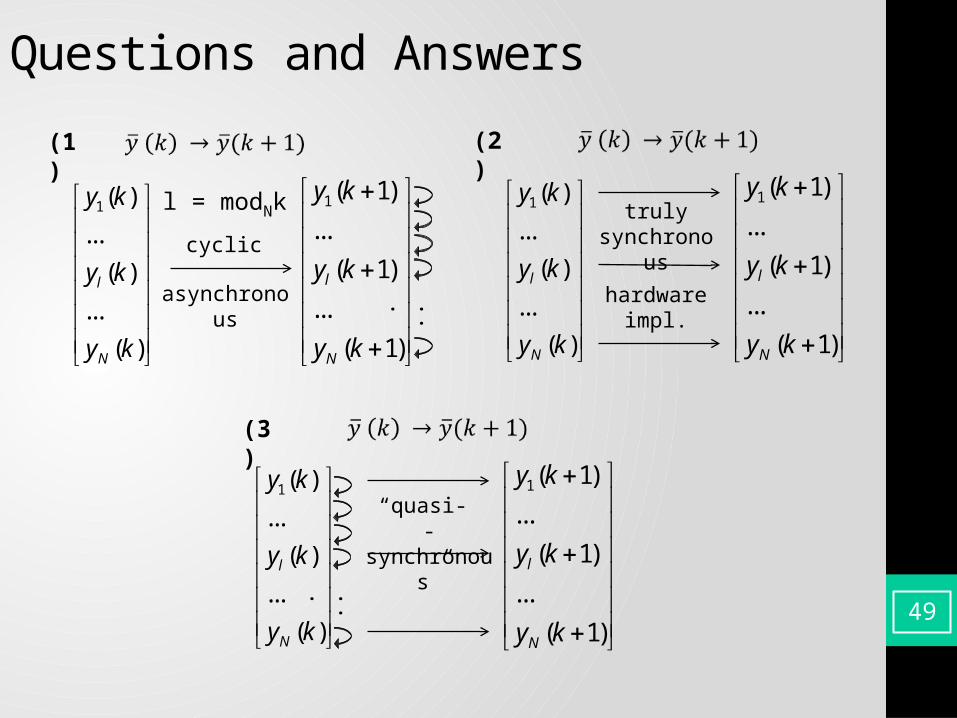
Q: Regarding the description of the HNN, the state transition rule is asynchronous, i.e. only one of the state variables (elements of vector y) is updated. What was the reason of using only asynchronous update instead of testing also synchronous one, which later would be more suitable for massively parallel implementations?

A:

• Synchronous updating implies updating nodes at exactly the same time (requires a “global clock tick” – unrealistic for biological/physical applications. R.Rojas: Neural Networks, Springer-Verlag, Berlin, 1996)

• On CPU’s only a “quasi-synchronous” implementation is possible (see next slide)

• Due to the inherent sequential updating and the storage/copying overhead, this implementation is slower than asynchronous updating on CPU’s

• For hardware-level implementation, indeed synchronous updating is faster, but this was not available and therefore, I put this beyond the scope of my dissertation (see pg. 57, paragraph 1)

Questions and Answers

 (2)

1( )

...

( )

...

( )

l

N

y k

y k

y k

1( 1)

...

( 1)

...

( 1)

l

N

y k

y k

y k

truly synchronoushardwareimpl.

1( 1)

...

( 1)

...

( 1)

l

N

y k

y k

y k

 (3)

1( )

...

( )

...

( )

l

N

y k

y k

y k

“quasi- -synchronous”

1( )

...

( )

...

( )

l

N

y k

y k

y k

1( 1)

...

( 1)

...

( 1)

l

N

y k

y k

y k

cyclicasynchronous

l = modNk (1)

...

49...