polyshrink: an adaptive variable selection procedure that
TRANSCRIPT

Polyshrink: An Adaptive Variable Selection Procedure
That Is Competitive with Bayes Experts
Dean P. Foster and Robert A. Stine ∗
The University of Pennsylvania
Department of Statistics
The Wharton School of the University of Pennsylvania
Philadelphia, PA 19104-6340
E-mail:{foster,stine}@wharton.upenn.edu
AbstractWe propose an adaptive shrinkage estimator for use in regression problems chara-
terized by many predictors, such as wavelet estimation. Adaptive estimators perform well over
a variety of circumstances, such as regression models in which few, some or many coefficients
are zero. Our estimator, PolyShrink, adaptively varies the amount of shrinkage to suit the esti-
mation task. Whereas hard thresholding using the risk inflation criterion is optimal for models
with few predictors, PolyShrink obtains a broader competitive optimality vis-a-vis the best
Bayes expert. A Bayes expert is the predictive distribution implied by a prior distribution for
the unknown coefficients. We derive non-asymptotic upper and lower bounds for the expected
log-loss, or divergence, of Bayes experts whose prior is unimodal and symmetric about zero.
Our bounds hold for any sample size and are pointwise in the sense that they hold for any
values of the unknown parameters. These bounds allow us to show that PolyShrink produces a
fitted model whose divergence lies within a constant factor of the divergence obtained by the
best Bayes expert. In a simulation of four frequently considered wavelet estimation problems,
PolyShrink obtains smaller mean squared error than hard thresholding, which is not adaptive,
and several other adaptive estimators.
Keywords and phrases: divergence, empirical Bayes, thresholding, relative entropy, wavelet.
1. Introduction
Consider the familiar problem of choosing the predictors in a regression model that is to be used to
predict future observations. Suppose that the response vector Y holds n independent observations
Y = (Y1, . . . , Yn). To model Y , we have access to a large collection of p ≤ n orthonormal predictors
arranged as the columns of an n × p matrix X = [X1, X2, . . . , Xp] with XtX = Ip. Assume that
these predictors affect the response through the standard linear model,
Yi = xtiβ + σεi, εi
iid∼ N(0, 1), i = 1, . . . , n, (1)
for arbitrary column vectors β, xi ∈ Rp, where xti is the ith row of X. The problem is to predict
accurately independent realizations of Y for known values of the predictors.∗The authors appreciate the helpful insights provided by the associate editor and referee.
1
imsart ver. 2005/05/19 file: bayes-expert.tex date: September 9, 2005

Foster and Stine/Adaptive variable selection 2
Table 1Average mean squared error of reconstructions of four test functions obtained in a simulation of hard thresholding
at√
2 log p, SureShrink, empirical Bayes thresholding (using exponential and Cauchy priors), and the proposedadaptive estimator. The standard error of each estimate is about 0.001, and differences within a column are
statistically significant.
Estimator Blocks Bumps HeaviSine Doppler
Hard(√
2 log p) 0.255 0.286 0.064 0.131SureShrink 0.219 0.247 0.064 0.127
Empirical Bayes (exp) 0.181 0.208 0.053 0.106Empirical Bayes (cau) 0.176 0.199 0.053 0.102
PolyShrink 0.172 0.193 0.052 0.100
Our interest focuses on problems in which p is roughly equal to n. This context is the standard
situation in, for example, harmonic analysis using a basis of sines and cosines or wavelets. This
context is also common, albeit with substantial collinearity, in data mining. In many of these
applications, the coefficients are sparse, “nearly black” in the language of Johnstone and Silverman
[15]. In these cases, most of the slopes βj = 0, implying the predictor Xj does not affect the
distribution of Y . Indeed, much of the motivation for wavelets owes to their ability to produce
sparse representations. Though it creates no bias to include predictors for which βj = 0, adding these
increases the variability of the fit. It should be remembered, however, that specification searches,
such as modern versions of stepwise regression, produce selection bias. Miller [16] provides a recent
survey of these results.
If the underlying model has known sparsity, then a variety of arguments motivate the following
thresholding estimator. Assume that σ2 = 1 is given and denote the least-squares estimators as
bj = XtjY ∼ N(0, 1). Our normalization of the regressors implies that the bj are standardized. The
hard thresholding estimator βH(τ)(b) sets to zero those bj which are smaller in size than a threshold
τ > 0,
βH(τ)j = bjI{|bj | ≥ τ} ,
where I{S} denotes the indicator function of the set S. Oracle inequalities [9], risk inflation [11],
data compression [12], and the classical Bonferroni rule all lead to the estimator βH(√
2 log p) (or
asymptotically similar soft-thresholding rules). This estimator includes in the model only those
predictors for which b2j > 2 log p, basically those for which the associated p-value is less than 1/p.
The problem with hard thresholding, of course, is that it is “too hard” when the underlying signal
spreads over more than a handful of basis elements.
Suppose, for example, that it is known that the pγ of the βj are zero. Rather than hard thresh-
olding at τ =√
2 log p, this knowledge might suggest setting the threshold to τγ =√
2 γ log p.
Abramovich et al. [1] observe that using the incorrect threshold τ1/2 when γ = 1/4 results in a
sixfold increase in the quadratic risk over that obtained by using τ1/4. To accommodate problems in
which β is sparse or dense, one would prefer an estimator that adapts to the problem, for example
by tuning the threshold.
imsart ver. 2005/05/19 file: bayes-expert.tex date: September 9, 2005
Foster and Stine/Adaptive variable selection 3
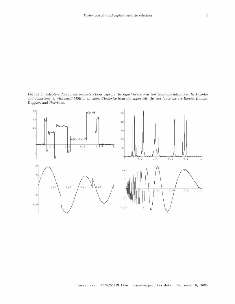
Figure 1. Adaptive PolyShrink reconstructions capture the signal in the four test functions introduced by Donohoand Johnstone [9] with small MSE in all cases. Clockwise from the upper left, the test functions are Blocks, Bumps,Doppler, and Heavisine.
0.2 0.4 0.6 0.8 1
-5
5
10
15
20
0.2 0.4 0.6 0.8 1
10
20
30
40
50
0.2 0.4 0.6 0.8 1
-10
-5
5
10
0.2 0.4 0.6 0.8 1
-10
-5
5
10
imsart ver. 2005/05/19 file: bayes-expert.tex date: September 9, 2005
Foster and Stine/Adaptive variable selection 4
To illustrate the benefits of adaptive estimation, consider estimating the four familiar test func-
tions introduced in Donoho and Johnstone [9]. These four functions have relatively sparse represen-
tations in a wavelet basis, but are visually distinct. One test function (called blocks) is piecewise
constant whereas another (heavisine) is rather smooth but for two discontinuities. Another has
a varying periodic structure (doppler), and the fourth has sharp spikes (bumps). Figure 1 shows
reconstructions using n = 2048 equally spaced observations of these signals. For each simulated
replication, we added random Gaussian noise with standard deviation σ = 1 to the underlying
signal. We scaled the test functions so that the standard deviation of the underlying signal equals
7, as in Donoho and Johnstone [9]. We obtained the estimates in the figure by using the adaptive
PolyShrink estimator that we define and study in the rest of this paper. The underlying signals
appear in gray, but the fits are so accurate that they obscure the test functions.
The accuracy of the PolyShrink reconstructions shown in Figure 1 is not accidental. PolyShrink
does well in general: it obtains smaller mean squared error than available alternatives for these
four test signals. Table 1 summarizes the simulated MSE over 250 replications obtained by five
estimators. The simplest, oldest and least accurate of these is the non-adaptive hard thresholding
estimator βH(√
2 log n) using the universal threshold√
2 log n ≈ 3.9. Whereas hard thresholding
uses a fixed threshold, the other four estimators use the least squares estimates to gauge the best
amount of thresholding to employ. In addition to PolyShrink we show results for two other adaptive
estimators:
SureShrink, which uses the soft-threshold that minimizes Stein’s unbiased estimate of risk [SURE,
8];
EbayesThresh, an empirical Bayes estimator that uses either a double exponential or Cauchy prior
[15];
The boxplots in Figure 2 compare the MSE obtained by the five estimators over the 250 simulated
samples. Though the boxplots overlap, the differences between mean values for each test function are
rather significant. For example when estimating blocks, even though the MSE of PolyShrink is only
0.004 less than that obtained by the empirical Bayes estimator using a Cauchy prior, this difference
produces a t-statistic larger than 15 because of the dependence between the estimates. (Each
estimator was applied to the same 250 realizations.) Of the five estimators, only hard thresholding,
the worst performing method, sets a common threshold over all resolutions of the wavelet transform.
The benefits of adaptation are clear. Unless the signal is very sparse, an estimator that adapts its
threshold to the signal at hand has smaller squared error.
Remark. For these computations, we used version 2.2.1 of R running on a macintosh computer. We
used the R packages waveslim to obtain the wavelet decompositions and ebayesthresh to compute
the empirical Bayes estimator. We chose the default values for parameters used by ebayesthresh.
imsart ver. 2005/05/19 file: bayes-expert.tex date: September 9, 2005

Foster and Stine/Adaptive variable selection 5
Figure 2. These boxplots compare the mean squared error of five estimators of the four test functions (clockwise,from upper left, are results for estimating blocks, bumps, doppler, and heavisine).
●
●
Hard Sure EB.exp EB.cau Poly
0.15
0.20
0.25
0.30
●
●
●
Hard Sure EB.exp EB.cau Poly
0.20
0.25
0.30
0.35
●●
●
●●●●●
●
●●● ●●●●●
Hard Sure EB.exp EB.cau Poly
0.04
0.06
0.08
0.10
0.12 ●
●●●
●●●
●
● ●
●●●
●●●
●
●
●
●
Hard Sure EB.exp EB.cau Poly
0.08
0.12
0.16
For filtering these wavelet coefficients (and comparison to other published simulations), we applied
thresholding only to the 6 levels of the LA8 wavelet coefficients (2016 coefficients with most localized
support). In practice, it may be quite hard to decide how many levels of the wavelet transform
to filter. The Polyshrink wavelet estimator has no tuning parameters, and we applied it to all
but the two, top-level wavelet coefficients. To avoid issues of various estimates of scale, for every
estimator we made use of the fact that σ = 1. An R package of our software is available at www-
stat.wharton.upenn.edu/∼stine and through the CRAN archive (cran.r-project.org).
The PolyShrink estimator β(b) adaptively thresholds its estimate of each coordinate. To con-
vey the nature of the adaption, Figure 3 shows β1(b), the estimator of β1, as a function of the
first element in the least squares estimator b. For this figure, we set the dimension p = 65.
The various curves in Figure 3 characterize how β1(b) changes with the size of the other coor-
dinates b2, . . . , b65. PolyShrink uses these other coordinates to adjust the amount of shrinkage
when estimating β1 from b1. To suggest the effect of signal in the other coordinates, we set
bj+1 = m + Φ−1(j/65), j = 1, . . . , 64, and varied m = 0, 1, 1.15, 1.25, 1.35, 2.0, as indicated in
the legend of the figure. At one extreme (the solid curve in the figure), there is no signal in the
other coordinates; their values are as though one has observed an idealized sample of pure Gaus-
imsart ver. 2005/05/19 file: bayes-expert.tex date: September 9, 2005

Foster and Stine/Adaptive variable selection 6
Figure 3. The adaptive Polyshrink estimator resembles hard thresholding with a large threshold when there is littlesignal and resembles soft thresholding with a small threshold when there is substantial signal. The curves show onecoordinate β1(b) for varying levels of signal spread over p = 65 coefficients.
−4 −2 0 2 4
−4
−2
02
4
b
Pol
yshr
ink(
b)
Signal Mean01.001.151.251.352.00
imsart ver. 2005/05/19 file: bayes-expert.tex date: September 9, 2005

Foster and Stine/Adaptive variable selection 7
sian noise. Such sparsity is commonly encountered when estimating the coefficients of wavelet basis
elements having most localized support. Heuristically, the absence of signal in the other coefficients
makes β1(b) “suspicious” of any signal found in b1, and so β1(b) heavily shrinks b1 toward zero.
Indeed, the plot of β1(b) resembles a smoothed version of the hard thresholding estimator with
a threshold slightly more than 2. As m increases, the other coordinates indicate the presence of
signal, and β1(b) offers less and less shrinkage. Once m = 2, β1(b) resembles a soft thresholding
estimator. Though not apparent in Figure 3, however, β1(b) returns to the diagonal as |b| increases.
Asymptotically in b1, the deviation is of order O(1/b1):
b1 − β(b1) ≈2b1
1 + b21.
The expressions that we use to compute β offer further insight into how the Polyshrink estimator
adapts. Although our theorems do not explicitly provide an estimator, an appendix describes the
conversion from the existential style of the theory to a more standard estimator. Assume as in
the orthogonal regression (1) that we observe observe a p-element vector of estimates b with mean
vector β and variance 1, b ∼ N(β, Ip). For wavelets, b denotes the standardized “raw” wavelet
transform at a given resolution, and β denotes the corresponding wavelet coefficients of the signal.
The PolyShrink estimator uses a collection of mixtures of the form
gεk(z) = (1− εk)φ(z) + εkψ(z) , εk = 2k−(K+1), k = 1, . . . ,K, (2)
where K = 1 + blog2 pc, φ(z) = exp(−z2/2)/√
2π is the standard normal density and ψ(z) =
1/(√
2π(1 + z2/2)) is a Cauchy density with scale√
2. The notation bxc denotes the greatest
integer less than or equal to x. The mixtures gεkplace larger weight on the Cauchy density as εk
increases. We extend gε to vector arguments by multiplication,
gε(b) = gε(b1)gε(b2) · · · gε(bp) .
With this notation in hand, the PolyShrink estimator is readily defined and computed. (An imple-
mentation in R requires about 20 lines of straightforward code.) Let wk = 2−kgεk(b) and normalize
these weights
wk = wk/K∑
i=1
wi , w = (w1, . . . , wK)t .
The normalized weights w allow βj to borrow strength from other coordinates when choosing an
appropriate amount of shrinkage. The PolyShrink estimator can then be written in the classical
style of Stein [18],
β = b+ S w , (3)
where the p×K matrix S holds the scores
Sjk =d
dzlog gεk
(z)|bj. (4)
imsart ver. 2005/05/19 file: bayes-expert.tex date: September 9, 2005

Foster and Stine/Adaptive variable selection 8
Thus β blends the score functions associated with mixtures gε. When there is little signal (illustrated
by the solid curve in Figure 3), the weights w concentrate in w1, placing the most emphasis on
the score function with the largest Gaussian component. In the calculations producing Figure 3,
w1 = 0.62 when m = 0. With signal present, the weights shift toward mixtures with a larger Cauchy
component. For example, with m = 1 this weight decreases to w1 = 0.46. With m = 2, the estimator
puts virtually all of its weight on the score function of g1/2, setting w1 ≈ 0 and w7 = 0.999.
The remainder of this paper develops the theoretical properties of the PolyShrink estimator. The
following section presents a more formal introduction that describes the origin of our estimator
and its properties. In particular, we explain our choice of a different type of loss function that
allows us to prove that the associated risk of β lies within a constant factor of the smallest risk
obtained by a class of Bayesian estimators that we call Bayes experts. Following in Section 3, we
offer some additional motivation by pointing out further connections to other estimators. In Section
4, we derive lower bounds for the risk of Bayes experts, and in Section 5, we describe the adaptive
estimator. We prove a key result, Theorem 2, in Section 6, and relegate further details of the proofs
to the second appendix. The first appendix describes the conversion from our theorems to the
PolyShrink estimator (3).
2. Competitive Analysis of Estimators
Consider the problem of predicting the next value of the response, Yn+1. The PolyShrink estimator
described in the introduction arises from the following competitive analysis. The goal is to find an
estimator that predicts as well the best expert who builds a prediction using side information that
would not be known to the statistician. This approach produces an adaptive estimator because
the estimator must do well as well as the best expert, regardless of the unknown parameters.
For example, one might seek a predictor Yn+1 = xn+1β whose expected squared prediction error
En+11 (Yn+1 − Yn+1)2 approaches that obtained by an expert who knows more than the data reveal
about the form of the model. (The expectation En+11 is over the joint distribution of the observable
response Y1, . . . , Yn and the future value Yn+1.) The extra information available to the expert might
come from an oracle that identifies the predictors that have non-zero coefficients as in Donoho and
Johnstone [9] or, less informatively, an oracle that reveals the number of non-zero coefficients.
For our analysis, the scope of the extra information lies somewhere between these alternatives:
an oracle provides a prior distribution π(β) for the regression coefficients. Given π, a Bayesian can
express uncertainty about the future value Yn+1 with the predictive distribution that encompasses
the posterior distribution of β. Denote the scalar density of the response associated with predictors
in the row vector x as
Pβ(y) = φ((y − xtβ)/σ
).
To simplify the notation, we omit x from the arguments of this function and leave this dependence
imsart ver. 2005/05/19 file: bayes-expert.tex date: September 9, 2005

Foster and Stine/Adaptive variable selection 9
implicit. We denote the predictive distribution of Yn+1 given Y by Pn+1π (y | Y ). This predictive
distribution is a Bayes expert in our terminology. In general, the predictive distribution for Yi+1
given Y1, . . . , Yi is
P i+1π (y | Y1, . . . , Yi) =
∫Pβ(y)π(β|Y1, . . . , Yi) dβ , i = 2, . . . , n, (5)
where
π(β | Y1, . . . , Yi)
denotes the posterior distribution of β given Y1, . . . , Yi. For the initial case that lacks prior data,
we define P 1π as
P 1π (y) =
∫Pβ(y)π(β) dβ .
It may seem that Bayes experts are little more than a collection of prior distributions, and so
one might question the need to introduce this terminology. While our notion of a Bayes expert does
employ a prior, our use of the word “expert” is meant to convey something more. An expert is any
prediction methodology, a map from the data to the space of new observations, that benefits from
information outside the scope of what would typically be available for estimation. We should also
point out that the objectives of our analysis differ from those that one would typically associate with
Bayesian analysis of a collection of priors. When confronted by a collection of priors, a Bayesian
might seek a method to elicit the best prior or to find a robust prior. We have a different objective.
Rather than seek the best Bayes estimator, we use Bayes estimators as a yardstick with which we
can judge the performance of adaptive variable selection.
We structure our competitive analysis around Bayes experts whose prior is unimodal and sym-
metric. We denote the class of priors by M. More precisely, the scalar distribution π ∈ M iff (1)
π is symmetric and (2) π assigns decreasing probability to intervals as the center of the interval
moves away from zero. Thus, if π ∈M and
pw(c) =∫ c+w
c−wdπ , w > 0, (6)
then pw(c) = pw(−c) and pw(c) is monotone decreasing on [0,∞]. In essence, the class M consists of
symmetric, unimodal densities that may possess an atom of probability at the origin. The assumed
orthogonality of the estimation problem allows us to extend π to vectors by multiplication, π(β) =
π(β1) · · ·π(βp). Thus π(0) reveals the expected number of elements of β that are zero. The rest of π
indicates how the signal distributes over the other coordinates. The choice of experts with π ∈ Mavoids artificial problems that would be caused by competing against super-efficient estimators. For
example, a realizable estimator cannot compete with an expert using a point-mass prior δ3(x) if in
fact βj = 3. The only point mass prior in M is δ0.
For a Bayes expert, a natural measure of accuracy is the expected log-probability loss or diver-
gence (relative entropy). We use D(f∥∥ g) to denote the divergence between the true density f and
imsart ver. 2005/05/19 file: bayes-expert.tex date: September 9, 2005

Foster and Stine/Adaptive variable selection 10
some other density g,
D(f∥∥ g) = Ef log
f(X)g(X)
=∫f(x) log
f(x)g(x)
dx . (7)
The divergence is well-defined if the support of g contains the support of f , and the assumed
normality of the errors in our model produces density functions with infinite support. The divergence
of a Bayes expert, the predictive distribution Pn+1π , from the distribution of Yn+1 is (suppressing
the dependence on xn+1)
L(β, Pn+1π ) = D
(Pβ
∥∥ Pn+1π
)=
∫log
Pβ(y)Pn+1
π (y | Y )Pβ(y) dy . (8)
Divergence has a long history in model selection. For example, AIC arose as an unbiased estimate
of the divergence [2]. The divergence can also resemble more familiar loss functions. For example, if
the posterior distribution concentrates near a point mass at, say, β then the divergence is roughly
quadratic,
L(β, Pn+1
π (y|Y ))≈
(xn+1(β(Y )− β)
)2
2σ2.
We depart from this approach to obtain our results on the competitive accuracy of Bayes ex-
perts. The loss function defined by (8) is a marginal loss in the sense that it describes the error
when predicting Yn+1 given xn+1 and information in the prior n observations. We obtain a more
analytically tractable quantity by replacing the marginal loss with the accumulated loss. Rather
than judge the expert by how well Pn+1π matches Pβ, we instead sum the deviations of P i
π from Pβ
for i = 1, . . . , n. Although one prefers an estimator that predicts well in the future over one that fits
well in the past (“Prediction is difficult, particularly about the future.”), we have found it easier
to prove theorems about the accumulated loss than the marginal loss. This change also removes
the dependence on the unknown xn+1, replacing it with the observed values of the predictors. The
product of these predictive distributions defines the prequential likelihood [5, 6]
Pπ(Y1, . . . , Yn) = P 1π (Y1)
n∏i=2
P iπ(Yi | Y1, . . . , Yi−1) .
The cumulative log-loss of a Bayes expert with prior π is then
Ln (β, Pπ) =n∑
i=1
logPβ(Yi)
P iπ(y | Y1, . . . , Yi−1)
. (9)
The expected value of Ln is the divergence of the prequential likelihood for Y . Thus, we define the
divergence risk obtained over the sequence of n predictions as
Rn (β, Pπ) ≡ En1 (Ln(β, Pπ))
= D(Pβ(Y )
∥∥ Pπ(Y )). (10)
imsart ver. 2005/05/19 file: bayes-expert.tex date: September 9, 2005

Foster and Stine/Adaptive variable selection 11
The success of the PolyShrink estimator summarized in the introduction suggests that the shift
from marginal to accumulated loss nonetheless produces a useful estimator.
We can now summarize our results for the PolyShrink estimator. Our first theorem provides non-
asymptotic lower bounds for divergence risk of Bayes experts whose prior distribution π ∈M, the
class of symmetric, unimodal priors. Theorem 1 also shows that, given a tuning constant ε(π) that
depends on the prior, there exists an an estimator gε(π)(π) whose divergence is within a constant
factor of that obtained by the best Bayes expert.
Theorem 1. For ε > 0, define the bounding function
B(β, ε) =p∑
j=1
min
(β2
j + ε,1β2
j
+ logβj
ε
). (11)
There exists a real-valued functional ε(π) such that, under the model (1) with p ≤ n orthonormal
predictors, the divergence risk (10) of any Bayes expert in the class M (see equation (6)) is bounded
below as follows:
(∀n,∀β, ∀π ∈M) Rn(β, Pπ) ≥ c B(β, ε(π)) , (12)
for some positive constant c < 1. Further, there exists an estimator gε(π) such that
(∀n,∀β,∀π ∈M) Rn(β, gε(π)) ≤ 2 B(β, ε(π)) (13)
We have numerically estimated the constant c ≈ 1/10, but it may be possible to close the gap
between (12) and (13) by using methods developed in Foster et al. [13].
The bounds in Theorem 1 reduce the problem of choosing a prior π ∈ M to the choice of a
number, ε. In fact, even the problem of picking ε can be eliminated as the following theorem shows.
Our second theorem describes an estimator g which in turn defines the PolyShrink estimator β
defined in (3) and described in the introduction. This estimator avoids the need for the functional
ε(π) in Theorem 1 by mixing gε over several values of ε. The weights in this mixture do not depend
on the prior π.
Theorem 2. There exists a distribution g (namely that implying the Polyshrink estimator) whose
divergence risk is a linear function of the best obtained by any Bayes expert whose prior π ∈ M(see equation (6)). In particular,
(∀n,∀β) Rn(β, g) ≤ ω0 + ω1 infπ∈M
Rn(β, Pπ) . (14)
3. Connections
Thresholding estimators possess a form of competitive optimality in the style of our theorems.
Let Qn(β, β) = En1
∑j(βj − βj(Y ))2 denote the quadratic risk of an estimator β. Donoho and
Johnstone [9] and Foster and George [11] show that the quadratic risk of the hard thresholding
imsart ver. 2005/05/19 file: bayes-expert.tex date: September 9, 2005
Foster and Stine/Adaptive variable selection 12
estimator βH(τ) using the universal threshold τ2 = 2 log p is bounded by a logarithmic factor of the
best possible. Abbreviating βH = βH(√
2 log p) then
Qn(β, βH) ≤ (2 log p+ 1) infβ∈S
Qn(β, β) , (15)
where S denotes the class of least-squares estimators based on selecting a subset of the predictors.
Donoho and Johnstone [9] introduce the notion of an oracle to describe the optimality of βH . Sup-
pose that a statistician can consult an oracle that indicates which elements of β to estimate. Then
the bound (15) shows that the quadratic risk of βH lies within a factor of 2 log p of that obtained
by consulting the best of all such coordinate oracles. Furthermore, this competitive performance
is the best possible vis-a-vis coordinate oracles. If we label the class of estimators based on these
oracles C, the class of coordinate experts, then we can state this result as:
(∀n,∀β) Qn(β, βH) ≤ ωQ(C)0 + ω
Q(C)1 inf
β∈CQn(β, β) .
where ωQ(C)1 = (1+2 log p). No variable selection procedure can do better than come within a factor
of log p of the quadratic risk attainable by coordinate experts.
We can contrast this with our result using the divergence risk and Bayes experts. A coordinate
expert knows which predictors to use in the regression and does not have to rely on data to decide
which coordinates to estimate. In contrast, Bayes experts are not so well-informed; each has only a
prior distribution for β from the class M. While useful, the prior is not so informative as knowing
which βj to estimate. In a sense, competing with Bayes experts resembles the comparison of two
estimators rather than the comparison of an estimator to the truth. Consequently, we can find a
data-driven procedure which is more competitive with Bayes experts than with coordinate experts:
(∀n,∀β) Rn(β, g) ≤ ω0 + ω1 infπ∈M
Rn(β, Pπ) ,
where we obtain an O(1) for ω1 bound instead of the O(log p) bound for ωQ(C)1 .
This comparison suggests the use of a different “ruler” to judge and compare estimators. No
data-driven estimator can come close to the performance of coordinate experts, so the alternatives
look equally good. Because we can come within a constant factor of the predictive risk of the Bayes
experts, however, we can hopefully use these as a more finely graduated ruler to separate better
estimators from others. Since Bayes estimators are admissible, a trivial lower bound for ratio of
risks is 1, and so our estimator lies within a constant of being optimal. Without the log p factor
inherent in the coordinate-based approach, we can begin the process of finding estimators that
reduce this constant.
An alternative approach to finding adaptive estimators considers their minimax properties. Our
theorems are point-wise in the sense we bound the divergence for each β with the divergence of
the best expert for that β. One obtains a uniform bound for every β by finding the minimax risk
imsart ver. 2005/05/19 file: bayes-expert.tex date: September 9, 2005

Foster and Stine/Adaptive variable selection 13
over some class of estimators and parameter spaces. Rather than do well for every β, a minimax
estimator need only be competitive for the hardest problems. Because the unconstrained minimax
quadratic risk for the regression model (1) is p, obtained by fitting every predictor, a non-trivial
minimax analysis must constrain the parameter space. Abramovich et al. [1] argue that a natural
constraint is to consider sparse problems in which few βj 6= 0 and restrict β to an `d ball for d
near zero. They show that this constraint leads to penalized estimators that do well over a range
of sparse problems. For example, let
Θ0n = {β : ‖β‖0 = n−δ}, where ‖β‖0 =
∑j
I{βj 6= 0}, δ > 0,
denote a nearly black parameter space in which β has few non-zero elements. The `0 norm ‖x‖0
counts the number of non-zero values in x. Let
R(Θ0n) = inf
βsup
β∈Θ0n
E‖β − β‖0
denote the corresponding minimax risk over all estimators β. Abramovich et al. [1] show that an
estimator βF derived from the false discovery rate of Benjamini and Hochberg [3] is asymptotically
minimax:
supβ∈Θ0
n
E‖β − βF ‖0 ≤ R(Θ0n)(1 + o(1)),
as n → ∞ for a suitable choice of the tuning parameter that controls the estimator. Whereas
Theorem 2 shows that the divergence risk of β is competitive for every β for all n, these results
show that the `0 risk of βF is asymptotically minimax.
Johnstone and Silverman [15] also consider the estimation problem in nearly black parameter
spaces. They show that an empirical Bayes estimator does well in both sparse problems as well as
when β is more dense. To this end, they consider empirical Bayes estimators with mixture priors
of the form h(x) = (1 − w)δ0(x) + w γ(x) where δ0(x) denotes a point mass at zero and γ(x) is a
symmetric, unimodal distribution, implying that the prior h(x) ∈M. [14, consider empirical Bayes
model selection in a more parametric setting.] As an estimator, they use the median of the posterior
distribution rather than a predictive distribution. The resulting estimator is thus very similar to
the PolyShrink estimator. For example, plots of their estimator [see Figure 5 of 15] resemble those
of the PolyShrink estimator in Figure 3. Also, the mean squared errors in the simulation reported
in the introduction are very similar. In the style of Abramovich et al. [1], they show that their
estimator has uniformly bounded risk over a wide range of parameter spaces and asymptotically
obtains the minimax risk. With an emphasis on the problem of estimating wavelets, Zhang [19]
extends and refines these results to a wider class of prior distributions and obtains a more precise,
though complex, collection of asymptotic properties.
imsart ver. 2005/05/19 file: bayes-expert.tex date: September 9, 2005

Foster and Stine/Adaptive variable selection 14
4. Lower Bounds for the Bayes Divergence
The results in this section and those that follow hold for the normal location model. These apply to
variable selection in regression since we can use an orthogonal rotation to convert the the slopes of
the orthonormal regression (1) into a vector of means. Let X = [X1, X2, . . . , Xp] denote the n× p
design matrix of the predictors. If we pre-multiply both sides of (1) by the transpose Xt, we obtain
Y = XtY ∼ N(β, σ2 In) . (16)
The question of which predictors to include then becomes one of deciding how to estimate the mean
vector β. Since σ2 is assumed known, we abuse our notation and further reduce the problem to the
following canonical form:
Yj ∼ N(µj , 1) , j = 1, . . . , p , independently. (17)
This reduction of a regression to a location problem is common in the analysis of variable selection
methods [e.g. 10]. The independence among the Yj allows us to work in the scalar setting.
We adopt the following notation. Write the normal density with mean µ by φµ(y) =
e−(y−µ)2/2/√
2π and abbreviate the standard normal density as φ0 = φ. The cumulative normal is
denoted Φ(x) =∫ x−∞ φ(t)dt. With these conventions, the distribution of Yi is
φµi(y) = φ(y − µi) .
Let H(φ) denote the entropy of the standard normal density,
H(φ) = −∫φ(y) log φ(y)dy = 1
2(1 + log 2π) . (18)
The marginal distribution for Yi implied by the prior π(µ) is
φπ(y) =∫φ(y − µ)π(µ)dµ . (19)
The one-dimensional divergence, viewed as a function of a scalar parameter µ, is
dπ(µ) ≡ D(φµ
∥∥ φπ)
=∫φµ(x) log
φµ(x)φπ(x)
dx . (20)
If we associate βj = µj and note that the prior factors as π(β) = π(β1) · · ·π(βp), then the divergence
risk defined in (10) may be written as
Rn(β, Pπ) =p∑
j=1
dπ(µj) . (21)
The following related examples suggest the properties of the divergence attainable by Bayes
experts. For µ ≈ 0, an expert with prior π(x) = δ0(x) (the indicator function at 0) performs well.
Its divergence is quadratic in µ,
dδ0(µ) = D(φµ
∥∥ φ0)
imsart ver. 2005/05/19 file: bayes-expert.tex date: September 9, 2005

Foster and Stine/Adaptive variable selection 15
Figure 4. Divergence of five spike-and-slab priors (23) with slab widths m that minimize the divergence dπ at µ =1, 2, 3, 4, 5 for fixed slab probability p = 0.05.
2 4 6 8 10Μ
2
4
6
8
10dΠ
=∫φ(y − µ) log
φ(y − µ)φ(y)
dy
= E Y 2/2 + 12 log 2π −H(φ)
= µ2/2 .
For a coordinate with non-zero parameter, the expert will achieve a lower divergence by placing
more probability away from zero. Let
Um(x) = 1[−m,m]/2m (22)
denote the uniform density on [−m,m]. The divergence for the expert that uses a uniform prior
out to |µ|+ 1 is
dU|µ|+1(µ) = D
(φµ
∥∥ φU|µ|+1
)≥ log 2(µ+ 1)−H(φ) .
Thus, the divergence for these experts is logarithmic. As a compromise, a spike-and-slab expert
(prior) combines these two extremes,
πp,m(µ) = (1− p)δ0(µ) + p Um(µ) . (23)
Figure 4 shows the divergence obtained with a sequence of five spike-and-slab priors whose slab
widths m minimize the divergence at µ = 1, 2, 3, 4, 5 for fixed slab probability p = 0.05. The lower
bounds for the divergence near zero grow quadratically, and then flatten to grow logarithmically
as µ increases.
Our lower bounds for dπ(µ) require a single functional of the prior. This functional measures the
ratio of how much probability φπ puts into a tail relative to the standard normal. To define this
functional, let rπ(τ) denote the ratio of tail integrals
rπ(τ) =∫∞τ φπ(y)dy∫∞τ φ0(y)dy
. (24)
imsart ver. 2005/05/19 file: bayes-expert.tex date: September 9, 2005

Foster and Stine/Adaptive variable selection 16
rπ(τ) is monotone increasing for τ > 0 because of the monotonicity of the likelihood ratio shown
in Lemma 5. Hence, for an arbitrary constant κ > 1, we can define the threshold
τκ(π) = infτ{τ : rπ(τ) > κ} . (25)
Given τκ(π), we define the needed functional to be the associated tail probability of φπ:
εκ(π) =∫ ∞
τκ
φπ(y)dy . (26)
Where it does not lead to ambiguity (since there is typically only one prior π under consideration),
we abbreviate εκ(π) as εκ. We shall also need the related tail integral of φ0:
δκ(π) =∫ ∞
τκ
φ0(y)dy = εκ(π)/κ . (27)
The threshold τκ(π) and tail area εκ(π) are equivalent in the sense that we can find one from the
other, without further knowledge of π, through the relationship
τκ(π) = −Φ−1(εκ(π)κ
)≈√
2 logκ
εκ(π). (28)
This approximation follows from the crude asymptotic equivalence Φ(−x) ≈ e−x2/2. Lemma 6
provides bounds on the approximation in (28) that are accurate to within 1 of the actual value.
Since rπ(0) = 1, we require κ > 1 so that τκ > 0 and εκ < 1/2.
Results in the Appendix show that the divergence of any Bayes model with prior π ∈ M grows
quadratically near the origin and eventually grows at a logarithmic rate. From the previous exam-
ples, we see that the divergence cannot be better than quadratic (as with a point mass at zero) or
logarithmic (obtained by the slab). Figure 5 shows the lower bounds for dπ(µ) from Lemma 15 with
the tuning parameter κ = e2 and εκ = 0.001. For reference, the figure denotes the location of the
threshold τκ with a short vertical line near µ = 3.6. The bounds shown in Figure 5 are, however,
rather hard to work with, and so we use a simpler set of bounds for our proofs. In Lemma 16, we
show that
∃λ > 0 s.t. ∀π ∈M : λ dπ(µ) ≥ min(µ2 + εκ(π),
1µ2
+ logµ
εκ(π)
)(29)
Though easier to work with, these simpler bounds retain the shape of the tighter bounds shown in
Figure 5. Namely, the bounds are quadratic for µ near 0 and grow logarithmically as µ moves away
from 0. Equation (29) implies the first statement of Theorem 1.
5. The Mixture Marginal
One estimator that achieves the upper bound given in Theorem 1 is a mixture of a normal density
with a Cauchy density. Let
ψ(y) =1√
2π(1 + y2/2)(30)
imsart ver. 2005/05/19 file: bayes-expert.tex date: September 9, 2005

Foster and Stine/Adaptive variable selection 17
Figure 5. Lower bounds from Lemma 15 are approximately quadratic in µ near the origin and grow logarithmicallyin µ for larger values of the parameter. The figure includes (in gray) the segments from the components of the lowerbound, with κ = e2 and εκ = 0.001. The vertical line near µ = 3.6 locates the position of τκ.
2 4 6 8 10Μ
1
2
3
4
5
6
dΠ
Figure 6. Divergence of the Cauchy mixture g0.001 and the lower bound for the divergence dπ(µ) attainable by aBayes prior with εκ(π) = 0.001.
2 4 6 8 10Μ
2
4
6
8
10
dΠ
denote the Cauchy density with scale√
2. This choice of scaling implies that the equivalent estimator
β(b) shown in Figure 3 is monotone increasing. Define a marginal distribution as a one-parameter
mixture of φ and ψ,
gε(y) = (1− ε)φ(y) + ε ψ(y) , 0 ≤ ε ≤ 1. (31)
For ε < 12 , Lemma 17 shows that the divergence of gε is bounded:
D(φµ
∥∥ gε)≤ 2 min{µ2 + ε, 1/µ2 + logµ/ε} . (32)
Equation (32) implies statement 2 of Theorem 1.
Figure 6 shows the upper bound for the divergence of gε with ε = 0.001. This plot includes
the lower bound for the divergence attainable by a Bayes expert with prior π ∈ M as shown in
Figure 5. The visual impression from the figure is that both bounds increase at comparable rates,
as demonstrated in the proof of Theorem 2 that follows in the next section.
imsart ver. 2005/05/19 file: bayes-expert.tex date: September 9, 2005

Foster and Stine/Adaptive variable selection 18
6. Proof of Theorem 2
This section provides a proof of Theorem 2, which we state here with more details than when it
was originally stated:
Theorem 2. Let K = 1 + blog2 pc. The sub-density
g(~y) = 12g(2−K)(~y) + 1
4g(2−K+1)(~y) + · · ·+ 2−K+1g(1/4)(~y) + 2−Kg(1/2)(~y)
=K∑
k=1
2−kg(2−(K+1−k))(~y) ,
where gε(~y) =∏gε(yj), and gε(yj) = (1− ε)φ(yj) + ε ψ(yj) has a risk function that is linear in the
best risk obtained by any unimodal prior. In particular,
(∀n,∀~µ)p∑
j=1
D(φµj
∥∥ g) ≤ ω0 + ω1 infπ∈M
p∑j=1
dπ(µj) .
Where equation (6) and (20) define M and dπ(·) respectively.
We set the constant κ defined in (25) to κ = e2 in the following derivations. This choice allows
us to absorb several constants into a multiple of dπ itself.
Lemma 1. Let gδ(y) = (1− δ)φ(y) + δ ψ(y). For any π ∈ M, if εκ(π) < δ ≤ 1/2, where εκ(π) is
defined in (26) then
D(φµ
∥∥ gδ
)≤ 2λ dπ(µ) + 2δ ,
Proof. From equation (32) we see that for δ > εκ(π),
D(φµ
∥∥ gδ
)≤ 2 min{µ2 + δ, 1/µ2 + logµ/δ}
≤ 2δ + 2 min{µ2, 1/µ2 + logµ/δ}
≤ 2δ + 2 min{µ2 + εκ(π), 1/µ2 + logµ/εκ(π)}
≤ 2δ + 2λdπ(µ) ,
where the last inequality comes from equation (29).
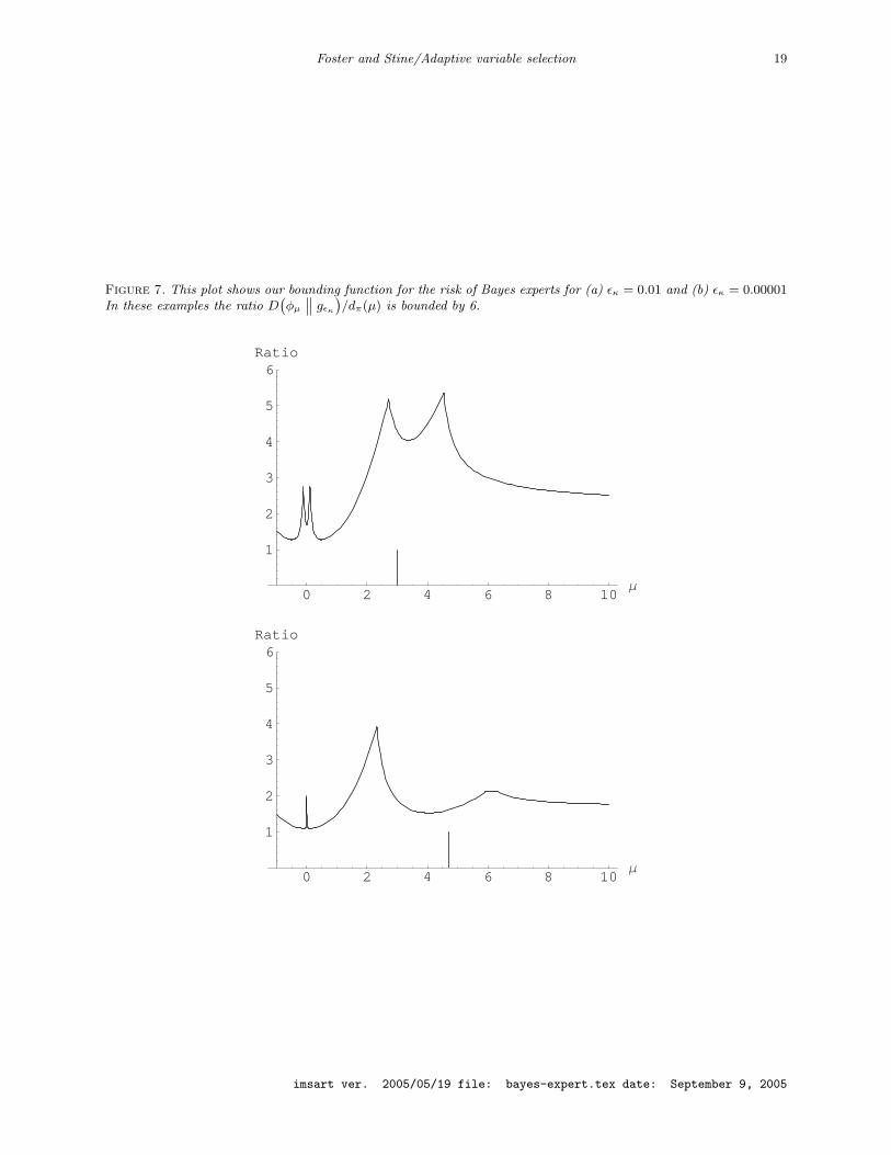
To clarify the arguments of our proofs, we have shown analytically that the bound obtains for
2λ = 10000. Numerical calculations suggest that the best coefficient is less than 6. To support this
claim, Figure 7 shows the ratio of the upper bound for D(φµ
∥∥ gεκ
)from Lemma 17 to the lower
bound for dπ(µ) from Lemma 15 for two choices of εκ, (a) εκ = 0.01 and (b) εκ = 0.00001, both over
the range −1 ≤ µ ≤ 10. In all cases shown (and others not pictured here) the ratio of divergences
D(φµ
∥∥ gεκ
)/dπ(µ) < 6.
To obtain practical results that apply in the multivariate problem, we have to remove δ from the
bound. The competitive bound continues to hold so long as the parameter δ indexing the marginal
distribution gδ is suitably close to εκ. At the same time, we can remove 2δ from the bound for
imsart ver. 2005/05/19 file: bayes-expert.tex date: September 9, 2005
Foster and Stine/Adaptive variable selection 19
Figure 7. This plot shows our bounding function for the risk of Bayes experts for (a) εκ = 0.01 and (b) εκ = 0.00001In these examples the ratio D
(φµ
∥∥ gεκ
)/dπ(µ) is bounded by 6.
0 2 4 6 8 10Μ
1
2
3
4
5
6Ratio
0 2 4 6 8 10Μ
1
2
3
4
5
6Ratio
imsart ver. 2005/05/19 file: bayes-expert.tex date: September 9, 2005

Foster and Stine/Adaptive variable selection 20
D(φµ
∥∥ gδ
)provided in Lemma 1 by increasing the size of the multiplier. For δ/2 ≤ εκ ≤ δ and
κ = e2, 1+log κκ ≤ 1
2 . Thus, the bound L0(µ, ε) of Lemma 15 becomes (see Lemma 11)
dπ(µ) ≥ εκ(1− 1 + log κκ
) ≥ εκ/2 .
Consequently, we have
D(φµ
∥∥ gδ
)≤ 2δ + 2λdπ(µ) ≤ 4εκ + 2λdπ(µ)
≤ (2λ+ 8)dπ(µ) . (33)
We handle separately the special case for εκ near zero where the previous bound no longer usefully
applies. Here, p is a positive integer that corresponds to the number of parameters in the regression
model. From Lemma 1, we obtain for εκ < δ < 1/(2p) that
D(φµ
∥∥ gδ
)≤ 2λ dπ(µ) + 1/p , (34)
where λ is the universal constant from Lemma 1.
From these results, we can extend the bounds on the ratio to problems in which Yi ∼ N(µi, 1),
i = 1, . . . , p. There is some δ such that 1/2p < δ = 2−k ≤ .5, and
D(φµi
∥∥ gδ
)≤ max[(2λ+ 8) dπ(µi), 2λdπ(µi) + 2/p]
≤ (2λ+ 8) dπ(µi) + 1/p , (35)
where we bound each such term for i = 1, . . . , p by either (33) or (34). Summing the individual
terms givesp∑
j=1
D(φµj
∥∥ gδ
)≤ 1 + (2λ+ 8)
∑j
dπ(µj) . (36)
The final step is to remove δ and obtain a universal model. We obtain a bound for the the divergence
of such a model in the following.
Lemma 2. Let Yi ∼ N(µi, 1), i = 1, . . . , p. There exists a density g such that
(∀π)p∑
i=1
D(φµi
∥∥ g) ≤ 2 + (2λ+ 12)p∑
i=1
dπ(µi) ,
where λ is the universal constant from Lemma 1.
Proof: Let k = dlog2 2pe. Let
g(y) =k∑
j=1
2−jg(2−(k+1−j))(y) .
Suppose εκ(π) < 1/(2p). First note that 2−k ≤ 1/(2p). Clearly
g(y) ≥ 12g(2−k)(y) . (37)
imsart ver. 2005/05/19 file: bayes-expert.tex date: September 9, 2005

Foster and Stine/Adaptive variable selection 21
Hence ∑i
D(φµi
∥∥ g) ≤ log 2 +∑
D(φµi
∥∥ g(2−k)
)≤ log 2 + 1 + 2λ
∑i
dπ(µi) ,
from equation (34), and our desired bound follows.
Now suppose εκ(π) ≥ 1/(2p). Let j be such that εκ(π) ≤ 2−(k+1−j) < 2εκ(π). We can bound the
divergence by ∑D(φµi
∥∥ g) ≤ j log 2 +∑
i
D(φµi
∥∥ g(2−(k+1−j))
)≤ j log 2 + (2λ+ 8)
∑dπ(µi) ,
where the second inequality follows from (36). Recalling that dπ(µ) ≥ εκ/2 we see that j log 2 <
2j ≤ 2p εκ < 4∑dπ(µi), and again we get the desired bound.
When we translate these divergences into risk notation (21), this Lemma implies Theorem 2.
Appendix: Calculating the estimator
The adaptive PolyShrink estimator β(b) shown in Figure 3 and used in the simulations approximates
the expectation of the model parameters. Because our model for the data summarized by the
function g in Theorem 2 does not use a typical parameterization, we obtain an equivalent estimator
by using a conditional expectation – a predictor. This predictor is constructed so that its expectation
is one of the model parameters.
We begin with a simple scalar problem, and then generalize the approach. Consider the scalar
estimation problem in which Y1, . . . , Yniid∼ N(µ, 1). Although our procedure does not produce an
estimator of µ per se, we obtain an approximate estimator as the conditional expectation
µ = Ef (Y1 | Y2, . . . , Yn) . (38)
The expectation that defines µ is with respect to the estimated joint density f(y1, . . . , yn) for the
data implied by our model.
To compute this estimator, we make use of a convenient orthogonal rotation that concentrates
µ into one coordinate. Let W denote an n× n orthogonal matrix that has the form
W =
1√n
√n−1
n 0 · · · 01√n
−√
1n(n−1) w23 · · · w2n
1√n
−√
1n(n−1) w33 · · · w3n
......
.... . .
...1√n
−√
1n(n−1) wn3 · · · wnn
imsart ver. 2005/05/19 file: bayes-expert.tex date: September 9, 2005
Foster and Stine/Adaptive variable selection 22
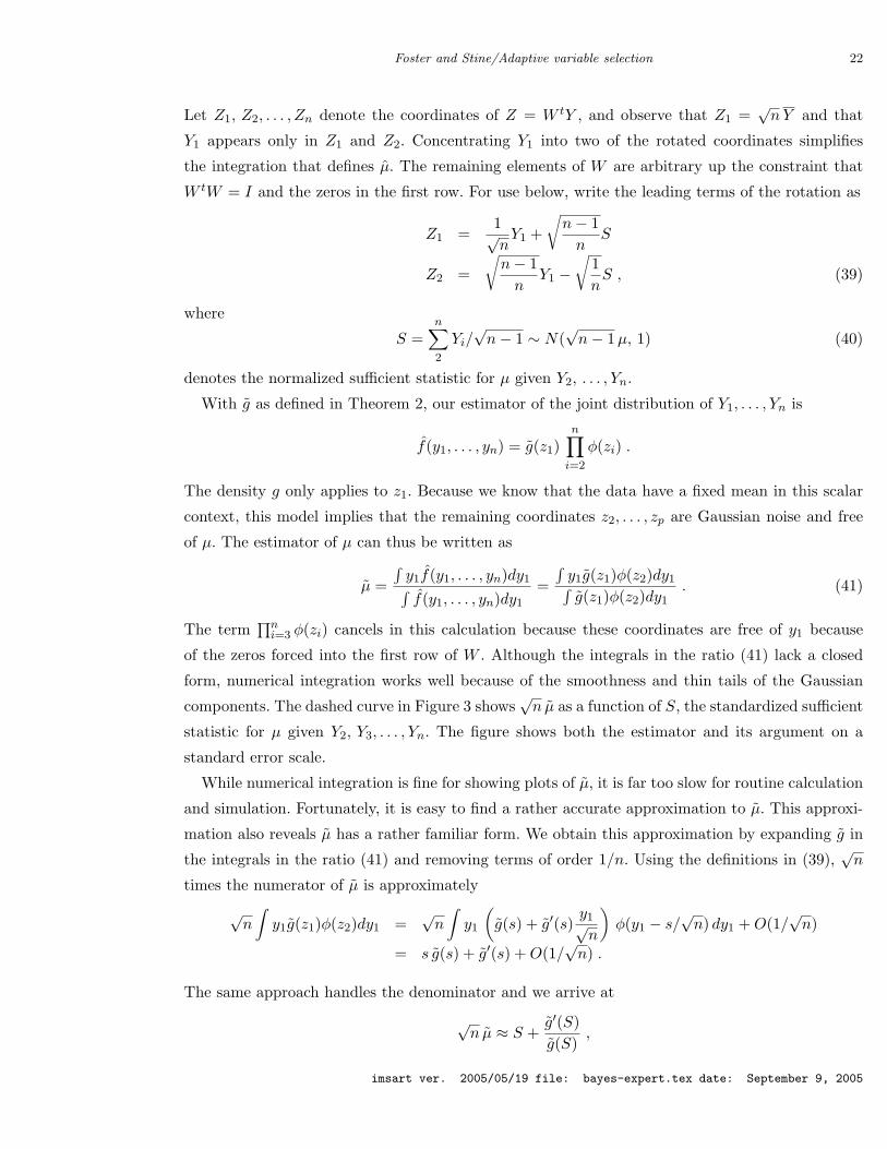
Let Z1, Z2, . . . , Zn denote the coordinates of Z = W tY , and observe that Z1 =√nY and that
Y1 appears only in Z1 and Z2. Concentrating Y1 into two of the rotated coordinates simplifies
the integration that defines µ. The remaining elements of W are arbitrary up the constraint that
W tW = I and the zeros in the first row. For use below, write the leading terms of the rotation as
Z1 =1√nY1 +
√n− 1n
S
Z2 =√n− 1n
Y1 −√
1nS , (39)
where
S =n∑2
Yi/√n− 1 ∼ N(
√n− 1µ, 1) (40)
denotes the normalized sufficient statistic for µ given Y2, . . . , Yn.
With g as defined in Theorem 2, our estimator of the joint distribution of Y1, . . . , Yn is
f(y1, . . . , yn) = g(z1)n∏
i=2
φ(zi) .
The density g only applies to z1. Because we know that the data have a fixed mean in this scalar
context, this model implies that the remaining coordinates z2, . . . , zp are Gaussian noise and free
of µ. The estimator of µ can thus be written as
µ =∫y1f(y1, . . . , yn)dy1∫f(y1, . . . , yn)dy1
=∫y1g(z1)φ(z2)dy1∫g(z1)φ(z2)dy1
. (41)
The term∏n
i=3 φ(zi) cancels in this calculation because these coordinates are free of y1 because
of the zeros forced into the first row of W . Although the integrals in the ratio (41) lack a closed
form, numerical integration works well because of the smoothness and thin tails of the Gaussian
components. The dashed curve in Figure 3 shows√n µ as a function of S, the standardized sufficient
statistic for µ given Y2, Y3, . . . , Yn. The figure shows both the estimator and its argument on a
standard error scale.
While numerical integration is fine for showing plots of µ, it is far too slow for routine calculation
and simulation. Fortunately, it is easy to find a rather accurate approximation to µ. This approxi-
mation also reveals µ has a rather familiar form. We obtain this approximation by expanding g in
the integrals in the ratio (41) and removing terms of order 1/n. Using the definitions in (39),√n
times the numerator of µ is approximately
√n
∫y1g(z1)φ(z2)dy1 =
√n
∫y1
(g(s) + g′(s)
y1√n
)φ(y1 − s/
√n) dy1 +O(1/
√n)
= s g(s) + g′(s) +O(1/√n) .
The same approach handles the denominator and we arrive at
√n µ ≈ S +
g′(S)g(S)
,
imsart ver. 2005/05/19 file: bayes-expert.tex date: September 9, 2005

Foster and Stine/Adaptive variable selection 23
with the partial sum S defined in (40). The remainder in the approximation is quite small. Once
n > 10 or so, plots of the approximate estimator are indistinguishable from those obtained by
numerical integration.
The case in which the regression parameter β is vector-valued provides an important insight into
the adaptive character of our estimator. To obtain a characterization similar to that provided for
the scalar estimator, we require some rather special assumptions on the basis. These conditions are
only needed to provide this characterization and do not affect, nor limit, the use of the estimator.
They simply allow us to isolate a single element of β. Assume now as in (1) that Yi ∼ N(xtiβ, I),
where β denotes an unknown p-element vector and the n row vectors xti combine to form an n× p
orthogonal matrix X. The p columns of are the first p columns of the n × n orthogonal matrix
W . Assume also that the first column of X is constant, so that the scalar example is a special
case. Let µ = β1. Assume further for convenience that x1,2 = · · · = x1,p = 0. For example, one
might have a sinusoidal basis in which the columns of X are given by the discrete Fourier basis,
xi,j = sin 2π(i − 1)(j − 1)/n for j = 2, . . . , p. As in the scalar case, assume that the remaining
noise coordinates confine the impact of Y1 by setting w1,p+2 = · · · = w1,n = 0, with w1,1 6= 0 and
w1,p+1 6= 0.
The equivalent adaptive estimator of µ is again a conditional expectation, only one with a more
complex model for the distribution of Y ,
µp = Efp[Y1|Y2, . . . , Yn] . (42)
To define fp, again let Z = W tY . Then
fp(y1, . . . , yn) = g(z1, . . . , zp)n∏
i=p+1
φ(zi) .
Because of the convenient choice of the basis, the expectation simplifies to a ratio of one-dimensional
integrals,
µp =∫y1g(z1, . . . , zp)φ(zp+1)dy1∫g(z1, . . . , zp)φ(zp+1)dy1
. (43)
Noting that g is a weighted sum of mixtures, set εj = 2−j and write
g(z1, . . . , zp) =k∑
j=1
εj gεk+1−j
(√n− 1n
s+ y1/√n, z2, . . . , zp)
)
=k∑
j=1
εj gεk+1−j
(√n− 1n
s+ y1/√n
) p∏i=2
gεk+1−j(zi)
Because of the position of zeros in the first row of W , the integration simplifies. Using the previous
expression for g(z1, . . . , zp) and the arguments that provide the scalar estimator, we obtain (with
k = dlog ne)√n
∫y1g(z1, . . . , zp)φ(zp+1)dy1
imsart ver. 2005/05/19 file: bayes-expert.tex date: September 9, 2005
Foster and Stine/Adaptive variable selection 24
=√n
k∑j=1
εj gεk+1−j(z2, . . . , zp)
∫y1gεk+1−j
(z1)φ(zp+1)dy1
=√n
k∑j=1
εj gεk+1−j(z2, . . . , zp)
∫y1gεk+1−j
(s+ y1/√n)φ(y1 − S/
√n)dy1 +O(1/
√n)
=k∑
j=1
εj gεk+1−j(z2, . . . , zp)
(s gεk+1−j
(s) + g′εk+1−j(s))
+O(1/√n)
=k∑
j=1
εj gεk+1−j(s, z2, . . . , zp)
(s+ g′εk+1−j
(s)/gεk+1−j(s))
+O(1/√n) .
Similarly, the denominator of µp reduces to∫g(z1, . . . , zp)φ(zp+1)dy1 =
k∑j=1
εj gεk+1−j(s, z2, . . . , zp) +O(1/n).
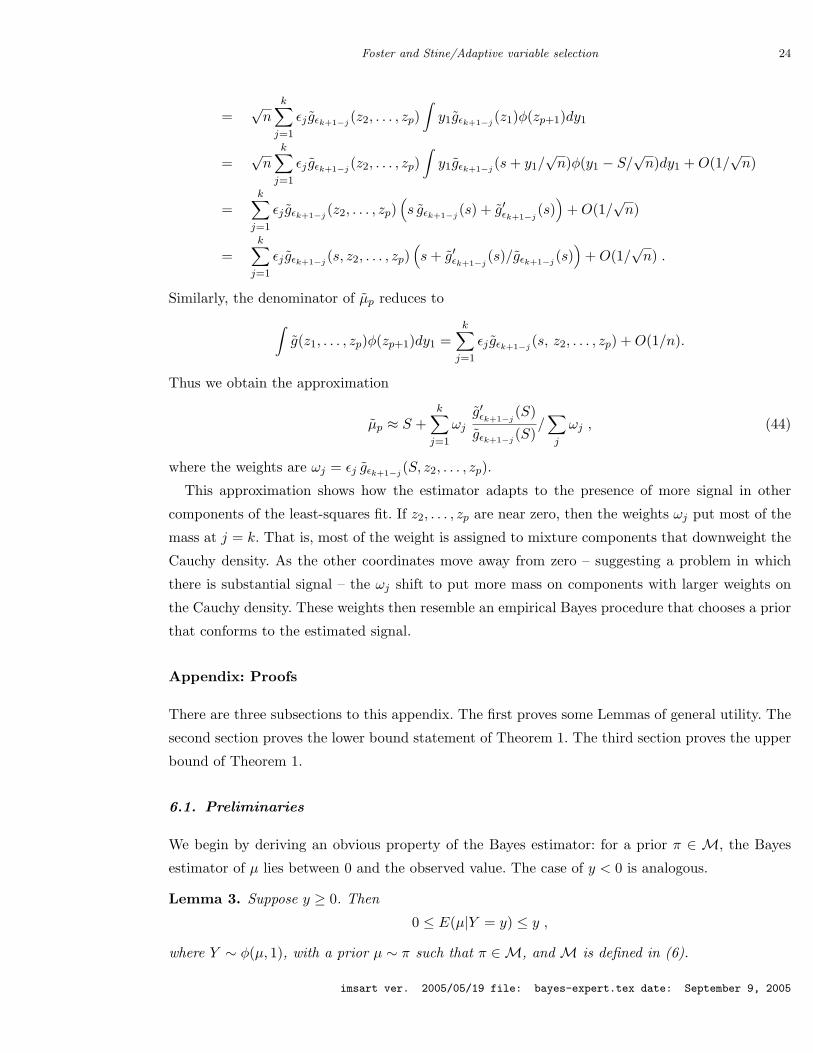
Thus we obtain the approximation
µp ≈ S +k∑
j=1
ωj
g′εk+1−j(S)
gεk+1−j(S)
/∑j
ωj , (44)
where the weights are ωj = εj gεk+1−j(S, z2, . . . , zp).
This approximation shows how the estimator adapts to the presence of more signal in other
components of the least-squares fit. If z2, . . . , zp are near zero, then the weights ωj put most of the
mass at j = k. That is, most of the weight is assigned to mixture components that downweight the
Cauchy density. As the other coordinates move away from zero – suggesting a problem in which
there is substantial signal – the ωj shift to put more mass on components with larger weights on
the Cauchy density. These weights then resemble an empirical Bayes procedure that chooses a prior
that conforms to the estimated signal.
Appendix: Proofs
There are three subsections to this appendix. The first proves some Lemmas of general utility. The
second section proves the lower bound statement of Theorem 1. The third section proves the upper
bound of Theorem 1.
6.1. Preliminaries
We begin by deriving an obvious property of the Bayes estimator: for a prior π ∈ M, the Bayes
estimator of µ lies between 0 and the observed value. The case of y < 0 is analogous.
Lemma 3. Suppose y ≥ 0. Then
0 ≤ E(µ|Y = y) ≤ y ,
where Y ∼ φ(µ, 1), with a prior µ ∼ π such that π ∈M, and M is defined in (6).
imsart ver. 2005/05/19 file: bayes-expert.tex date: September 9, 2005

Foster and Stine/Adaptive variable selection 25
Proof:
Write φ = φ0. The lower bound is obvious by partitioning the expectation as
φπ(y)E(µ|y) =∫µφ(y − µ)π(µ) dµ
=∫ 0
−∞µφ(y − µ)π(µ) dµ+
∫ ∞
0µφ(y − µ)π(µ) dµ
=∫ ∞
0−µφ(y + µ)π(µ) dµ+
∫ ∞
0µφ(y − µ)π(µ) dµ
=∫ ∞
0µ (φ(y − µ)− φ(y + µ))π(µ) dµ
≥ 0 .
The upper bound comes from a similar partitioning argument. The idea is to remove most of the
integral by use of the symmetry around 0 of φ and φπ. For this purpose, define
π(µ) =
π(µ) µ > y ,
π(2y − µ) µ ≤ y ,
which is symmetric around y. Thus,∫(y − µ)φ(y − µ)π(µ) dµ = 0. With this definition, we have
φπ(y)E(y − µ|Y = y) =∫
(y − µ)φ(y − µ)π(µ) dµ
=∫
(y − µ)φ(y − µ) (π(µ)− π(µ)) dµ
=∫ y
−∞(y − µ)φ(y − µ) (π(µ)− π(µ)) dµ
≥ 0
since all of the terms in the integral are positive for µ < y.
The second preliminary result that we show establishes the monotonicity of the divergence of
the Bayes mixture.
Lemma 4. The divergence dπ(µ) (defined in equation (20)) is monotone increasing as µ moves
away from 0. That is, for |µ0| < |µ1|,
dπ(|µ0|) < dπ(|µ1|) .
where dπ(·) is
Proof:
Since dπ(µ) = dπ(−µ), we need only consider the case 0 < µ0 < µ1. Define the midpoint ζ =
(µ0 + µ1)/2. Then
dπ(µ1)− dπ(µ0) =∫φ(y − µ0) log φπ(y) dy −
∫φ(y − µ1) log φπ(y) dy
=∫φ(u) log φπ(u+ µ0) du−
∫φ(u) log φπ(u+ µ1) du
=∫ ∞
ζφ(u) log
φπ(u+ µ0)φπ(u+ µ1)
du−∫ ζ
−∞φ(u) log
φπ(u+ µ1)φπ(u+ µ0)
du
imsart ver. 2005/05/19 file: bayes-expert.tex date: September 9, 2005

Foster and Stine/Adaptive variable selection 26
=∫ ∞
0φ(u− ζ) log
φπ(u+ µ0 − ζ)φπ(u+ µ1 − ζ)
du−∫ ∞
0φ(−u− ζ) log
φπ(µ1 − ζ − u)φπ(µ0 − ζ − u)
du
=∫ ∞
0(φ(ζ − u)− φ(ζ + u)) log
φπ(u+ (µ0 − µ1)/2)φπ(u+ (µ1 − µ0)/2)
du
> 0 ,
since both factors in the final integral are positive over the range of integration.
We will also need the following property of the likelihood ratio.
Lemma 5. The likelihood ratio of φπ(y)/φ0(y) is monotone increasing for y > 0:
d
dy
φπ(y)φ0(y)
> 0 . (45)
Proof. Assume y > 0. Differentiating under the integral, we have
d
dy
φπ(y)φ0(y)
=φ0(y)φ′π(y)− φπ(y)φ′0(y)
φ20(y)
=φ0(y) (
∫µφ(y − µ)π(µ)dµ− yφπ(y)) + yφ0(y)φπ(y)
φ20(y)
=∫µφ(y − µ)π(µ)dµ
φ0(y)> 0 ,
because of the monotonicity of the Bayes estimator shown in Lemma 3.
The following Lemma offers a more precise version of the approximation given in (28). We do
not exploit the accuracy of this approximation and include it here for completeness.
Lemma 6. √−2 log εκ + log(2/π)− 2 log κ− 1 ≤ τκ ≤
√−2 log εκ + log(2/π)− 2 log κ
and:2κe−(τκ+1)2/2
√2π
≤ εκ ≤2κe−τ2
κ/2
τ√
2πProof:
εκ = 2κΦ(−τ) ≤ 2κφ0(τ)/τ ≤2κe−τ2/2
τ√
2π.
The other direction is
εκ = 2κΦ0(−τ) ≥ 2κφ0(τ + 1) ≥ 2κe−(τ+1)2/2
√2π
.
For τκ > 1, these show that
log εκ ≤ 12 log(2/π) + log κ− τ2/2
log ε− 12 log(2/π)− log κ ≤ −τ2/2
−2 log ε+ log(2/π) + 2 log κ ≥ τ2√−2 log ε+ log(2/π) + 2 log κ ≥ τ
imsart ver. 2005/05/19 file: bayes-expert.tex date: September 9, 2005

Foster and Stine/Adaptive variable selection 27
For the other bound, we have:
log ε ≥ 12 log(2/π) + log κ− (τ + 1)2/2
2 log ε ≥ log(2/π) + 2 log κ− (τ + 1)2
2 log ε− log(2/π)− 2 log κ ≥ −(τ + 1)2√−2 log ε+ log(2/π)− 2 log κ− 1 ≤ τ
6.2. Lower Bounds
This section proves equation (12) which is the lower bound statement of Theorem 1.
Our first Lemma is a direct consequence of the monotonicity of dπ and the well-known relationship
between the L1 norm and the divergence. This Lemma shows that dπ (defined in equation (20)) lies
above a simple function of the cumulative normal distribution Φ. This bound is useful for dπ(µ) for
values of µ ≈ 1. Since the bound provided by this Lemma goes to 0 as µ→ 0 and is itself bounded
by 1/(2 log 2), we need to improve it for both small and large values of the parameter.
Lemma 7.
dπ(µ) ≥ (2Φ(µ)− 1)2
2 log 2.
Proof. It is well known that the divergence is bounded below by a multiple of the L1 norm [for
example, see 4]
D(f∥∥ g) ≥ 1
2 log 2‖f − g‖2
1 . (46)
The monotonicity of dπ established in Lemma 4 shows that
dπ(µ) ≥ max(dπ(µ), dπ(0))
= max(D(φµ
∥∥ φπ), D(φ0
∥∥ φπ)) .
Now using the L1 bound from (46), we obtain
dπ(µ) ≥ 12 log 2
max(‖φµ − φπ‖2
1, ‖φ0 − φπ‖21
)≥ 1
8 log 2‖φµ − φ0‖2
1 ,
where the last step uses the triangle inequality for the L1 norm,
‖a− c‖1 = ‖a− b+ b− c‖1 ≤ ‖a− b‖1 + ‖b− c‖1 ≤ 2 max(‖a− b‖1, ‖b− c‖1) .
The expression in the statement of the Lemma comes from noting that the L1 distance between
two normal densities is
‖φµ − φθ‖ = 2(
2Φ( |µ− θ|
2
)− 1
).
imsart ver. 2005/05/19 file: bayes-expert.tex date: September 9, 2005
Foster and Stine/Adaptive variable selection 28
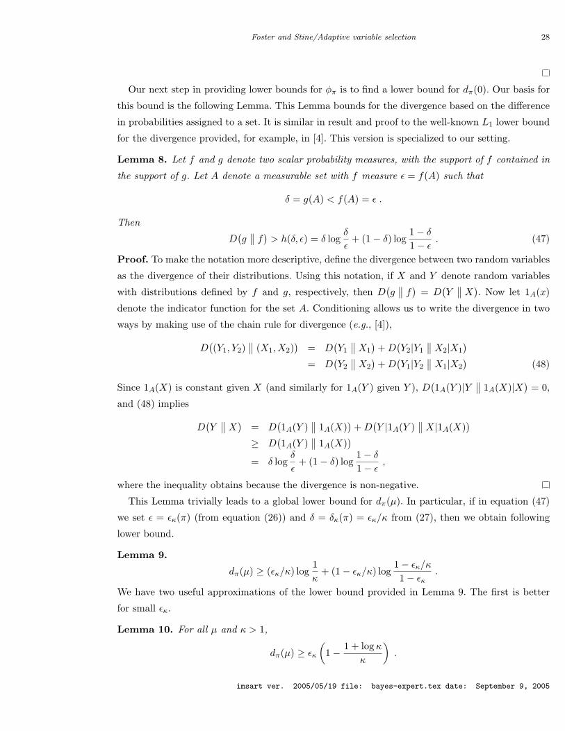
Our next step in providing lower bounds for φπ is to find a lower bound for dπ(0). Our basis for
this bound is the following Lemma. This Lemma bounds for the divergence based on the difference
in probabilities assigned to a set. It is similar in result and proof to the well-known L1 lower bound
for the divergence provided, for example, in [4]. This version is specialized to our setting.
Lemma 8. Let f and g denote two scalar probability measures, with the support of f contained in
the support of g. Let A denote a measurable set with f measure ε = f(A) such that
δ = g(A) < f(A) = ε .
Then
D(g∥∥ f) > h(δ, ε) = δ log
δ
ε+ (1− δ) log
1− δ
1− ε. (47)
Proof. To make the notation more descriptive, define the divergence between two random variables
as the divergence of their distributions. Using this notation, if X and Y denote random variables
with distributions defined by f and g, respectively, then D(g∥∥ f) = D
(Y∥∥ X). Now let 1A(x)
denote the indicator function for the set A. Conditioning allows us to write the divergence in two
ways by making use of the chain rule for divergence (e.g., [4]),
D((Y1, Y2)
∥∥ (X1, X2))
= D(Y1
∥∥ X1)+D
(Y2|Y1
∥∥ X2|X1)
= D(Y2
∥∥ X2)+D
(Y1|Y2
∥∥ X1|X2)
(48)
Since 1A(X) is constant given X (and similarly for 1A(Y ) given Y ), D(1A(Y )|Y
∥∥ 1A(X)|X)
= 0,
and (48) implies
D(Y∥∥ X) = D
(1A(Y )
∥∥ 1A(X))+D
(Y |1A(Y )
∥∥ X|1A(X))
≥ D(1A(Y )
∥∥ 1A(X))
= δ logδ
ε+ (1− δ) log
1− δ
1− ε,
where the inequality obtains because the divergence is non-negative.
This Lemma trivially leads to a global lower bound for dπ(µ). In particular, if in equation (47)
we set ε = εκ(π) (from equation (26)) and δ = δκ(π) = εκ/κ from (27), then we obtain following
lower bound.
Lemma 9.
dπ(µ) ≥ (εκ/κ) log1κ
+ (1− εκ/κ) log1− εκ/κ
1− εκ.
We have two useful approximations of the lower bound provided in Lemma 9. The first is better
for small εκ.
Lemma 10. For all µ and κ > 1,
dπ(µ) ≥ εκ
(1− 1 + log κ
κ
).
imsart ver. 2005/05/19 file: bayes-expert.tex date: September 9, 2005
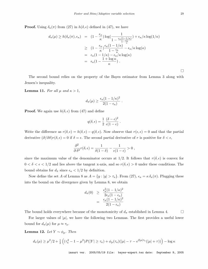
Foster and Stine/Adaptive variable selection 29
Proof. Using δκ(π) from (27) in h(δ, ε) defined in (47), we have
dπ(µ) ≥ h(δκ(π), εκ) = (1− εκκ
) log(1
1− εκ(1−1/κ)1− εκ
κ
) + εκ/κ log(1/κ)
≥ (1− εκκ
)εκ(1− 1/κ)
1− εκκ
− εκ/κ log(κ)
= εκ(1− 1/κ)− εκ/κ log(κ)
= εκ(1− 1 + log κκ
) .
The second bound relies on the property of the Bayes estimator from Lemma 3 along with
Jensen’s inequality.
Lemma 11. For all µ and κ > 1,
dπ(µ) ≥ εκ(1− 1/κ)2
2(1− εκ).
Proof. We again use h(δ, ε) from (47) and define
q(δ, ε) =12
(δ − ε)2
ε(1− ε).
Write the difference as r(δ, ε) = h(δ, ε) − q(δ, ε). Now observe that r(ε, ε) = 0 and that the partial
derivative (∂/∂δ)r(δ, ε) = 0 if δ = ε. The second partial derivative of r is positive for δ < ε,
∂2
∂ δ2r(δ, ε) =
1δ(1− δ)
− 1ε(1− ε)
> 0 ,
since the maximum value of the denominator occurs at 1/2. It follows that r(δ, ε) is convex for
0 < δ < ε < 1/2 and lies above the tangent x-axis, and so r(δ, ε) > 0 under these conditions. The
bound obtains for dπ since εκ < 1/2 by definition.
Now define the set A of Lemma 8 as A = {y : |y| > τκ}. From (27), εκ = κ δκ(π). Plugging these
into the bound on the divergence given by Lemma 8, we obtain
dπ(0) ≥ ε2κ(1− 1/κ)2
2εκ(1− εκ)
=εκ(1− 1/κ)2
2(1− εκ)
The bound holds everywhere because of the monotonicity of dπ established in Lemma 4.
For larger values of |µ|, we have the following two Lemmas. The first provides a useful lower
bound for dπ(µ) for µ ≈ τκ.
Lemma 12. Let Y ∼ φµ. Then
dπ(µ) ≥ µ2/2 + 12
((τ2
κ − 1− µ2)P (|Y | ≥ τκ) + φµ(τκ)(|µ| − τ − e2|µ|τκ(|µ|+ τ)))− log κ
imsart ver. 2005/05/19 file: bayes-expert.tex date: September 9, 2005

Foster and Stine/Adaptive variable selection 30
Proof. As in the prior proof, let A = {y : |y| < τκ} and let Ac denote its complement. The proof
of this Lemma is a direct evaluation of the divergence, with the inequality obtained by exploiting
the monotonicity of φπ(|y|) and the definition of τκ in (25). This definition implies φπ(y) < κφ0(y)
for |y| < τκ.
dπ(µ) =∫
log1
φπ(y)φµ(y)dy −H(φ)
≥∫
Alog
1κφ0(y)
φµ(y)dy +∫
Aclog
1κφ0(τκ)
φµ(y)dy −H(φ) ,
since φπ(τκ) = κφ0(τκ). Collecting terms, we have
dπ(µ) ≥ 12
∫min(y2, τ2
κ)φµ(y)dy + 12 log 2π −H(φ)− log κ
= 12
(∫Ay2φµ(y)dy + τ2
κP (|Y | ≥ τκ))− 1
2 − log κ ,
since H(φ)− 12 log 2π = 1/2. Solving the integral in somewhat closed form and collecting constants
give the lower bound for dπ(µ) as claimed in the Lemma.
We use a separate result to bound dπ(µ) for larger |µ|. The proof of this Lemma is an application
of the so-called data-processing inequality to the random variable Y ∨ µ− δ where Y ∼ φπ.
Lemma 13. For arbitrary δ, set α = Φ(−δ). Then for |µ| ≥ δ,
dπ(µ) ≥ (1− α) log1
φπ(|µ| − δ)+ α logα−H(φ) . (49)
Proof. Assume µ > δ and split the divergence dπ(µ) into two parts,
dπ(µ) =∫φµ(y) log
φµ(y)φπ(y)
dy
=∫
y≤µ−δφµ(y) log
φµ(y)φπ(y)
dy +∫
y>µ−δφµ(y) log
φµ(y)φπ(y)
dy .
Let A denote the event {Y ≤ µ− δ}. Let φµ(y|A) and φπ(y|A) denote the conditional probability
measures, and define φπ(A) =∫A φπ(x)dx. The first term of the divergence can be analyzed using
a conditioning argument.∫y≤µ−δ
φµ(y) logφµ(y)φπ(y)
dy =∫
y≤µ−δαφµ(y|A) log
αφµ(y|A)φπ(y|A)φπ(A)
dy
= α logα
φπ(A)+ α
∫y≤µ−δ
φµ(y|A) logφµ(y|A)φπ(y|A)
dy
≥ α logα
φπ(A)≥ α logα . (50)
The second term can be analyzed more directly using the monotonicity of φπ:∫y>µ−δ
φµ(y) logφµ(y)φπ(y)
dy ≥ −H(φ) +∫
y>µ−δφµ(y) log
1φπ(y)
dy
imsart ver. 2005/05/19 file: bayes-expert.tex date: September 9, 2005

Foster and Stine/Adaptive variable selection 31
≥ −H(φ) +∫
y>µ−δφµ(y) log
1φπ(µ− δ)
dy
= −H(φ)− (1− α) log φπ(µ− δ) . (51)
With the bounds (50) and (51) combined, we arrive at the lower bound as stated.
To make use of this Lemma, we remove the Bayes mixture φπ from (49) and replace it with a
simple function of εκ defined in (26). Assume µ > τκ + δ. Then we can bound φπ(µ− δ) from above
by
φπ(µ− δ) <εκ
µ− δ − τκ. (52)
because the tail area εκ is greater than the area of a rectangle of height φπ(µ − δ) and width
2(µ− δ − τκ). Putting the bound for φπ from (52) into (49) gives the following Lemma:
Lemma 14. For |µ| > τκ + δ, define α = Φ(−δ). Then
dπ(µ) ≥ (1− α) log|µ| − δ − τκ
εκ+ α logα−H(φ) . (53)
The choice of δ remains. Clearly one would like to choose δ so as to maximize the bound in (53).
Although we can numerically find a value of δ that maximizes this bound, the expression as offered
is too complex to allow an explicit solution. However, if we assume δ is of moderate size, we can
approximate the bound in (53) as
h(δ) = Φ(δ) log(µ− δ − τκ) . (54)
If we then set (∂/∂δ)h(δ) = 0 and drop constants and terms of smaller size, we arrive at an
approximately optimal choice of δ. If we write the solution as a function of µ and the threshold,
then the approximate optimal choice is δ(µ, τκ) where
δ(µ, τ) =√
2 log(µ− τ) for µ > τ + 1 , (55)
and zero otherwise. The following Lemma collects several bounds for dπ(µ) from Lemma 7, Lemma
9 and Lemma 14.
Lemma 15.
dπ(µ) ≥ L(µ, εκ)
where
L(µ, ε) = max{L0(µ, ε), L1(µ), L2(µ, ε), L3(µ, ε)} , (56)
where the bounding functions are
L0(µ, ε) = (εκ/κ) log1κ
+ (1− εκ/κ) log1− εκ/κ
1− εκ,
L1(µ) =(2Φ(µ)− 1)2
2 log 2,
imsart ver. 2005/05/19 file: bayes-expert.tex date: September 9, 2005

Foster and Stine/Adaptive variable selection 32
L2(µ, ε) = 12
(∫Ay2φµ(y)dy + τ2
κP (|Y | ≥ τκ)− 1)− log κ
and
L3(µ, ε) = (1− α) log|µ| − δ − τκ
εκ+ α logα−H(φ),
where in L3 we assume |µ| > δ + τκ and set α = Φ(−δ).
A simpler form of these bounds facilitates our comparison of the expert divergence dπ to that
obtained by the predictive model g. Though the bounds are not so tight as those just laid out, they
are adequate to show the existence of finite ratios.
Lemma 16. For κ = e2:
∃λ > 0 s.t. ∀π ∈M : λ dπ(µ) ≥ min
(µ2
i + εκ(π),1µ2
i
+ logµi
εκ(π)
)
Proof. We proceed by simplifying the bounds for various ranges of µ, starting with those near 0.
Case A: (µ2 ≤ εκ) For κ = e2, 1+log κκ ≤ 1
2 . Thus, Lemma 11 gives
dπ(µ) ≥ εκ(1− 1 + log κκ
) ≥ εκ/2 ≥ µ2/4 + εκ/4
= (µ2 + εκ)/4 . (57)
So any λ > 4 will work.
Case B: (εκ ≤ µ2 ≤ 9) For µ in this range, (2Φ(µ) − 1)2 ≥ µ2/10. Thus, the L1 bound from
Lemma 7 gives
dπ(µ) ≥ (2Φ(µ)− 1)2
2 log 2≥ µ2
20 log 2≥ µ2/2 + εκ/2
20 log 2≥ (µ2 + εκ)/(40 log 2) (58)
So any λ > 40 log 2 will work.
Case C: (9 ≤ µ2 ≤ τ2κ/2) We simplify the L2(µ, ε) bound by replacing the expectation Eµ(Y 2∧τ2
κ)
by something more manageable, here a truncated linear function that is tangent to the quadratic.
Recalling log κ = 2, we obtain
L2(µ, ε) = 12
(∫Ay2φµ(y)dy + τ2
κP (|Y | ≥ τκ) + log 2π)−H(φ)− log κ
≥ 12
∫(y ∧ µ)2φµ(y)dy − 5/2
≥ 12
∫max[0,min(τ2
κ , µ(2y − µ))]φµ(y)dy − 5/2
≥ µ2
∫max[−τ2
κ/µ,min(τ2κ/µ, (2y − µ))]φµ(y)dy − 5/2
= µ2/2− 5/2
imsart ver. 2005/05/19 file: bayes-expert.tex date: September 9, 2005

Foster and Stine/Adaptive variable selection 33
≥ µ2/2− 5/2 ,
since max(−τ2κ/µ,min(τ2
κ/µ, (2y − µ))) is an odd function centered at µ.
For µ > 3 we see that
(µ2 − 5)/2 > µ2/10 + 1 > µ2/10 + ε/10
so our bounds apply with λ = 10.
Case D: (τ2κ/2 ≤ µ2 ≤ 72τ2
κ) By monotonicity of dπ (see Lemma 4), we know that for µ in this
range dπ(µ) > dπ(τκ/√
2) = (τ2κ + ε)/20. At the upper limit for this range, we must have
72τ2κ + ε ≤ λ(τ2
κ + ε)/20 ,
so λ ≥ 1440 will work.
Notice that if τκ is less than 3 (and hence the previous case holds vacuously) we still achieve this
bound by appealing to the case before that. This means λ ≥ 72 ∗ 40 log 2 = 5760 log 2 will suffice.
Case E: (72τ2κ ≤ µ2) First note that τκ >
√2 for κ = e2. If we set δ = Φ−1(.9) ≈ 1.28 in the
bound L3(µ, ε) given in Lemma 15, then for this range of µ:
dπ(µ) ≥ 0.9 logµ− τκ − δ
εκ+ 0.1 log 0.1−H(φ)
≥ 0.1 logµ− τκ − δ
εκ+ 0.8 log[2(6
√2− 1)
√2− δ] + 0.1 log 0.1−H(φ)
≥ 0.1 logµ− τκ − δ
εκ+ 0.8 log 18 + 0.1 log 0.1−H(φ)
≥ 0.1 log 1/εκ + 0.1 log(µ− τκ − δ) + 0.66
≥ 0.1 log 1/εκ + 0.1 log µ+ 0.1 logµ− τκ − δ
µ+ 0.66
≥ 0.1 log 1/εκ + 0.1 log µ+ 0.1 log(6√
2− 1)τκ − δ
6√
2τκ+ 0.66
≥ 0.1 log 1/εκ + 0.1 log µ+ 0.6 (59)
Since for µ ≥ 1 we have that .6 ≥ .1/µ2, we can write the lower bound as dπ(µ) ≥ 0.1 log µ/εκ +
0.1/µ2 since µ is bigger than 1. Thus, any λ ≥ 10 will work for this case.
In summary, any λ ≥ 5760 log 2 will prove our desired result.
6.3. Upper Bounds
Lemma 17. For gε(y) = (1− ε)φ(y) + εψ(y)
D(φµ
∥∥ gε)≤ min{µ2/2− log(1− ε), logµ2π + 3/µ2 − log(ε)−H(φ)} .
Proof. Begin by bounding the divergence as the minimum of the divergence of either density used
to define gε:
D(φµ
∥∥ gε)
= D(φµ
∥∥ (1− ε)φ0 + εψ)
imsart ver. 2005/05/19 file: bayes-expert.tex date: September 9, 2005
Foster and Stine/Adaptive variable selection 34
≤ min(D(φµ
∥∥ (1− ε)φ0), D(φµ
∥∥ ε ψ)) .The first term is easy:
D(φµ
∥∥ (1− ε)φ0)
= D(φµ
∥∥ φ0)− log(1− ε) = µ2/2− log(1− ε) .
The second piece is less straightforward. First write
D(φµ
∥∥ ε ψ) = D(φµ
∥∥ ψ)− log(ε) .
We can bound the divergence between the Gaussian and the scaled Cauchy, ψ(z) = 1/(√
2π(1 +
z2/2)), as follows,
D(φµ
∥∥ ψ) =∫φµ(y) log
φµ(y)ψ(y)
dy
=∫φµ(y) log(π
√1/2(2 + y2))dy −H(φ)
= log(µ2 + a)π/√
2 +∫φ(z) log
(1 +
2µz + z2 + 2− a
µ2 + a
)dy −H(φ)
Using the bound log(1 + x) ≤ x and a = 3 we get a bound on the divergence of D(φµ
∥∥ ψ) ≤log(µ2 + 3)π
√2−H(φ) ≤ logµ2 + log π
√2 + 3/µ2 −H(φ).
The following Lemma is weaker than the above bound but simpler to work with theoretically. It
proves the second statement of Theorem 1.
Lemma 18. If ε < .5, then for gε(y) = (1− ε)φ(y) + εψ(y)
D(φµ
∥∥ gε)≤ 2 min{µ2 + ε, 1/µ2 + logµ/ε} .
Proof. We show this by bounding each term in Lemma 17 separately. The first term is bounded
above by
µ2/2− log(1− ε) ≤ µ2/2 + (3/2)ε
≤ 2µ2 + 2ε ,
where the first inequality follows from the restriction that ε ≤ .5. The second term is bounded as:
logµ2π + 3/µ2 − log(ε)−H(φ) = 2 logµ+ log π + 3/µ2 − log(ε)− (log 2πe)/2
= 2(
logµ
ε+ 1/µ2
)+(
1/µ2 + log ε+(log π/2e)
2
)≤ 2
(log
µ
ε+ 1/µ2
)+(1/µ2 + log ε
)If µ ≥
√log 2 andε ≤ 1/2 then 1/µ2 + log ε is less than zero and the bound follows. If µ ≤ 1, then
µ2 + ε is the binding term and we have our desired result. Further, if ε < e−4, and 1 ≤ µ ≤ 2 the
µ2 + ε is again binding. For the region e−4 ≤ ε ≤ 1/2 and 1 ≤ µ ≤ 2 a look at a graph generated
by numerical calculation is sufficient to see that the bound holds over that region.
imsart ver. 2005/05/19 file: bayes-expert.tex date: September 9, 2005

Foster and Stine/Adaptive variable selection 35
References
[1] Abramovich, F., Benjamini, Y., Donoho, D. and Johnstone, I. (2000). Adapting to un-
known sparsity by controlling the false discovery rate. Tech. Rep. 2000–19, Dept. of Statistics,
Stanford University, Stanford, CA.
[2] Akaike, H. (1973). Information theory and an extension of the maximum likelihood principle.
In B. N. Petrov and F. Csaki, eds., 2nd International Symposium on Information Theory. Akad.
Kiado, Budapest.
[3] Benjamini, Y. and Hochberg, Y. (1995). Controlling the false discovery rate: a practical
and powerful approach to multiple testing. Journal of the Royal Statist. Soc., Ser. B 57
289–300.
[4] Cover, T. M. and Thomas, J. A. (1991). Elements of Information Theory. Wiley, New
York.
[5] Dawid, A. P. (1984). Present position and positional developments: some personal views,
statistical theory, the prequential approach. Journal of the Royal Statist. Soc., Ser. A 147
278–292.
[6] Dawid, A. P. (1992). Prequential analysis, stochastic complexity and bayesian inference. In
J. M. Bernardo, J. O. Berger, A. P. Dawid and A. F. M. Smith, eds., Bayesian Statistics 4.
Oxford University Press, Oxford.
[7] Donoho, D. (2002). Kolmogorov complexity. Tech. rep., Stanford University, Stanford, CA.
[8] Donoho, D. and Johnstone, I. M. (1995). Adapting to unknown smoothness via wavelet
shrinkage. Journal of the Amer. Statist. Assoc. 90 1200–1224.
[9] Donoho, D. L. and Johnstone, I. M. (1994). Ideal spatial adaptation by wavelet shrinkage.
Biometrika 81 425–455.
[10] Efron, B. (2001). Selection criteria for scatterplot smoothing. Annals of Statistics 29 470–
504.
[11] Foster, D. P. and George, E. I. (1994). The risk inflation criterion for multiple regression.
Annals of Statistics 22 1947–1975.
[12] Foster, D. P. and Stine, R. A. (1996). Variable selection via information theory. Tech.
Rep. Discussion Paper 1180, Center for Mathematical Studies in Economics and Management
Science, Northwestern University, Chicago.
[13] Foster, D. P., Stine, R. A. and Wyner, A. J. (2002). Universal codes for finite sequences
of integers drawn from a monotone distribution. IEEE Trans. on Info. Theory 48 1713–1720.
[14] George, E. I. and Foster, D. P. (2000). Calibration and empirical bayes variable selection.
Biometrika 87 731–747.
[15] Johnstone, I. M. and Silverman, B. W. (2004). Needles and straw in haystacks: empirical
Bayes estimates of possibly sparse sequences. Annals of Statistics 32 1594–1649.
imsart ver. 2005/05/19 file: bayes-expert.tex date: September 9, 2005

Foster and Stine/Adaptive variable selection 36
[16] Miller, A. J. (2002). Subset Selection in Regression (Second Edition). Chapman& Hall,
London.
[17] Rissanen, J. (1983). A universal prior for integers and estimation by minimum description
length. Annals of Statistics 11 416–431.
[18] Stein, C. M. (1981). Estimation of the mean of a multivariate normal distribution. AS 9
1135–1151.
[19] Zhang, H.-C. (2005). General empirical Bayes wavelet methods and exactly adaptive minimax
estimation. Annals of Statistics 33 54–100.
imsart ver. 2005/05/19 file: bayes-expert.tex date: September 9, 2005