popularity functions for the french president and … · popularity functions for the french...

HAL Id: halshs-00872313https://halshs.archives-ouvertes.fr/halshs-00872313

Submitted on 11 Oct 2013

HAL is a multi-disciplinary open accessarchive for the deposit and dissemination of sci-entific research documents, whether they are pub-lished or not. The documents may come fromteaching and research institutions in France orabroad, or from public or private research centers.

L’archive ouverte pluridisciplinaire HAL, estdestinée au dépôt et à la diffusion de documentsscientifiques de niveau recherche, publiés ou non,émanant des établissements d’enseignement et derecherche français ou étrangers, des laboratoirespublics ou privés.

Popularity Functions for the French President andPrime Minister (1995-2007)

Antoine Auberger

To cite this version:Antoine Auberger. Popularity Functions for the French President and Prime Minister (1995-2007).2011. <halshs-00872313>

https://halshs.archives-ouvertes.fr/halshs-00872313

https://hal.archives-ouvertes.fr

1

Popularity Functions for the French President and

Prime Minister (1995-2007)

ANTOINE AUBERGER

1 March 2011

In this article, we study popularity functions for the French President and Prime Minister. We

show that the responsibility hypothesis is validated for the unemployment rate but not for the

inflation rate. We also show that voters have not a behavior compatible with the rational

expectations hypothesis for the Prime Minister’s popularity, and that voters have an

asymmetric behavior for the unemployment rate. We show the influence of political variables

which can depend on Prime Minister changes, the domestic political situation and

international political events.

Keywords: Popularity Functions • Voters’ Behavior • Economy • Politics • Econometric

Models

IRGEI LARGEPA, University Panthéon-Assas (Paris 2), 7 rue de la grande chaumière, 75006 – Paris, France. Tel:

33(1)40510418. E-mail: [email protected]. This work was partially made when the author was a member of the

LAEP, University Panthéon-Sorbonne (Paris 1). The author thanks the participants of the European public choice conference

(Jéna, March 27-30, 2008) for their comments on a previous version of this work and the participants of the seminar of the

IRGEI LARGEPA (Paris, June 25, 2010).

mailto:[email protected]

2

Introduction

Since the beginning of the 1970s and the first articles of Mueller (1970) for the United States

(popularity of the American president) and of Goodhart and Bhansali (1970) for Great Britain

(popularity of the British political parties), numerous studies showed the significant influence

of the economic situation on the popularity of the President and the political parties. It is a

subject of research for the public choice school.1

The popularity functions allow us to explain the popularity of those in power (President,

Prime Minister) and the political parties. They have an economic part and a political part. The

most used economic variables are the rates of inflation and unemployment.2 The GNP or GDP

real growth and the gross disposable household income are also used. Generally, economic

variables depend on the economic situation (objective measure), but they can possibly depend

on the perception of the economic situation by voters (subjective measure). Political variables

can depend on election cycles: honeymoon effect or depreciation of the popularity (the

popularity of those in power is high after an election or an appointment, and then regularly

decreases), the personality of those in power (personal factors). Frey and Schneider (1978),

notably, used a variable taking into account the depreciation of popularity for each American

President. International events3, wars (as the Vietnam war for the United States) or domestic

events (as the Watergate scandal for the United States) can have an influence on the

popularity of those in power. The political context can also have an influence on the

popularity of those in power. Finally, political variables can depend on economic policy

decisions. Generally speaking, as highlighted by Nannestad and Paldam (1994), the economic

part of the popularity functions is better studied than the political one; furthermore, the

popularity functions are rather unstable over time.4

There were also for France some studies showing the significant influence of the economic

situation on the French President’s and Prime Minister’s popularity. In many studies about the

French President’s or Prime Minister’s popularity, unemployment (unemployment rate or

unemployment level) was a significant economic variable. For example, Lewis-Beck (1980)

showed the significant influence of the monthly unemployment level with a lag of two months

on the President’s and Prime Minister’s popularity (over the period 1960-1978). In the studies

over the period 1960-19835, inflation (inflation rate or its change) was a significant economic

variable. For example, Lafay (1984) showed the significant influence of the semestrial

inflation rate on the President’s popularity. Other economic variables are used as the real

disposable household income by Lafay (1984), and real wages by Lecaillon (1984) because

voters are sensitive to change in their purchasing power. Political variables can depend on the

election cycles: honeymoon effect and/or depreciation in the popularity as in Courbis (1995).

Political variables can also depend on international or domestic events: notably the scandals

as in Lafay and Servais (2000) or the strikes as in Dubois (2005), the political context:

relations between the President and the Prime Minister as in Hibbs (1981), decisions of

economic policy as the Barre plan in Lafay (1984).

1 Mueller (2003) made a complete and updated presentation of public choice; we shall notably find in this book a synthesis

of the influence of the various economic variables on the popularity of those in power and of the political parties for several

countries. 2 We mostly use their lagged variables, that is the previous data to the surveys’ poll institutes.

3 Mueller (1970) used a “rally round the flag” variable.

4 According to Lafay (1981), the bad specification of these functions and, in particular, political variables is a cause of this

instability. 5 Since the middle of the 1980s, the inflation was curbed in France.

3

In this article, we build, and estimate popularity functions for the French President and

Prime Minister over the period 1995:6-2007:4 with the SUR (model of seemingly unrelated

regressions) technique.6 We show that the change in the unemployment rate has a significant

influence on the popularity of the French President and Prime Minister (responsibility

hypothesis) but not the change in the inflation rate. For the popularity of the President, we

also study the hypothesis of a partial responsibility of the President for the economic situation

(change in the unemployment rate) during the period of cohabitation (1997:6-2002:4). For the

President’s and Prime Minister’s popularity, we show the influence of political variables,

which are dependent on the popularity cycles as Prime Minister changes (popularity of Prime

Minister), the domestic political situation: strikes, the crisis of the FCE (first contract

employment), scandals, international events (conflict in Kosovo, terrorist attempts of 11

September 2001), the 1998 football world cup. We show that the unexpected change in the

unemployment rate has a significant influence on the President’s popularity, but that it has not

a significant influence on the Prime Minister’s popularity, and that voters have an asymmetric

behavior for the change of the unemployment rate, but that they have not partisan behavior.

After presenting the various analyses concerning the voters’ behavior (section 2), we

present the data used in this study over the period 1995:5-2007:4 (section 3); and then the

empirical analysis with the study of the influence of the objective and subjective economic

situation, the expected and unexpected objective economic situation, the hypothesis of

asymmetric behavior, and partisan behavior of voters (section 4). Finally, we make a

conclusion (section 5).

The microeconomic foundations of the popularity functions and the voters’ behavior

The construction and the estimate of popularity functions are implicitly made with some

hypotheses for the voters’ behavior. Downs (1957) supposed that voters are rational, that is

every voter votes for the candidate or the party which will give him the highest utility. Voters

should thus have forward-looking behavior, that is to support the government according to

their future personal situation (“egotropic” behavior). In fact, in many economic popularity

models, voters are supposed to have retrospective behavior. Furthermore, they are often

supposed to be myopic (they only take into account the recent economic situation).7 They

behave according to the responsibility hypothesis of Paldam (1981), that is they support the

government if they are satisfied with the economic situation, and punish it in the opposite

case; it corresponds to the “reward-punishment” behavior of Key (1966).8 Moreover, voters

are often supposed to evaluate the economic performances with the objective general

economic situation (“sociotropic” behavior). Both types of behavior (“sociotropic” and

“egotropic”) can however be difficult to be distinguished because good (resp. bad) economic

performances often have some positive (resp. negative) consequences on every voter. Lewis-

Beck and Paldam (2000) noticed that, usually, voters have “sociotropic” behavior.

Numerous authors as Frey and Schneider (1978), Hibbs (1982) and Haynes (1995) used a

retrospective model to estimate a popularity function. According to Lewis-Beck and Paldam

(2000), voters have more retrospective behavior than forward-looking behavior but the

difference between these two models is weak.

6 Veiga and Veiga (2004) used this econometric technique in their study of the popularity functions in Portugal.

7 On the other hand, Hibbs (1981,1982) supposed that voters take into account the economic situation on the whole

presidential term of office; he however supposed that voters attach more importance to the recent economic results. 8 On the other hand, Hibbs (1981,1982) found that voters take into account the economic performances of those in power in a

relative way by comparing them with the previous in power.

4

Swank (1990, 1993, 1995) developed for the United States a model where voters have

partisan preferences as in the theory of the partisan political cycle of Hibbs (1987): in periods

of high inflation, a right-wing party in power may see its popularity increase if voters think

that the priority of economic policy is the fight against inflation; in periods of increasing

unemployment, a left-wing party in power may see its popularity increase if voters think that

the priority of the economic policy is the fight against unemployment. Swank found favorable

results for this model with the popularity of the American President. Carlsen (2000) also

found favorable results for the partisan behavior (unemployment) with the right-wing

governments (the United States, Great Britain, Canada and Australia). Letterie and Swank

(1997), and Swank (1998), developed a more complete model in which are competency

(responsibility) economic variables and partisan economic variables included. Empirical

results are favorable to their model for the popularity of the American President.

The model of asymmetric behavior was originally developed for the vote function in the

elections of the American Congress by Bloom and Price (1975). Voters are supposed to have

asymmetric behavior: they reward a government for good economic performances less than

they punish it for bad economic results. Headrick and Lanoue (1991) found unfavorable

results for the asymmetric behavior for Great Britain (government popularity).

Several authors studied if the voters’ behavior was compatible with the rational

expectations hypothesis (voters are rational and efficiently use the information). According to

this hypothesis, only unexpected changes in economic variables have an influence on the

popularity of the President, government and political parties. A model of voters’ behavior

with rational expectations was developed by Holden and Peel (1985), inspired by the article of

Hall (1978) for the consumption function. The rational expectations hypothesis was accepted

by Holden and Peel (1985) for Great Britain and confirmed by Chrystal and Peel (1986) for

several countries; but rejected (at least partially) by Kirchgässner (19859, 1991) for Germany,

Price and Sanders (1994) for Great Britain and Neck and Karbuz (1997) for Austria.

Cho and Young (1992) showed that voters do not consider the American President

responsible for the expected inflation, and that they have asymmetric behavior for the

unexpected inflation: the American President is more punished for an increase in the

unexpected inflation than he is rewarded for a decline in the unexpected inflation.

The data

We begin by making a quick presentation of the French political system.10

The President of

the Republic is the head of State, he appoints the Prime Minister and mainly is in charge of

Foreign Policy and Defence. The government, led by the Prime Minister, decides on the

policy of France. Traditionally, the President of the Republic and the Prime Minister belong

to the same political side. When the opposite occurs, we speak about periods of cohabitation.

Except in periods of cohabitation, the President of the Republic determines the nation’s

policy, while during the periods of cohabitation, the Prime Minister is fully at the head of the

government.

During the studied period (1995:5-2007:4), Jacques Chirac was the President of the Republic

(May 7, 1995- May 6, 2007). He was elected on May 7, 1995 and reelected on May 5, 2002.

During the seven-year term of office of Jacques Chirac (1995-2002), Alain Juppé was the

Prime Minister (May 17, 1995- June 2, 1997) and then, Lionel Jospin was the Prime Minister

9 Kirchgässner (1985) showed the influence of the unexpected unemployment and inflation rates for the German political

parties’ popularity. 10

We partially use again the presentation of the French political system of Auberger and Dubois (2005).

5

(June 2, 1997- May 6, 2002). Thus, there was during five years (1997-2002) a period of

cohabitation with a right-wing President of the Republic and a left-wing Prime Minister.

During the five-year term of office of Jacques Chirac (2002-2007), Jean-Pierre Raffarin was

the Prime Minister (May 6, 2002- May 31, 2005) and then, Dominique de Villepin was the

Prime Minister (May 31, 2005- May 15, 2007).

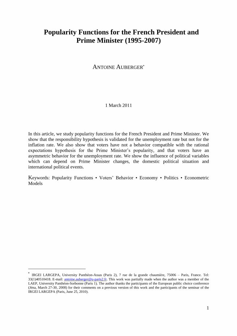
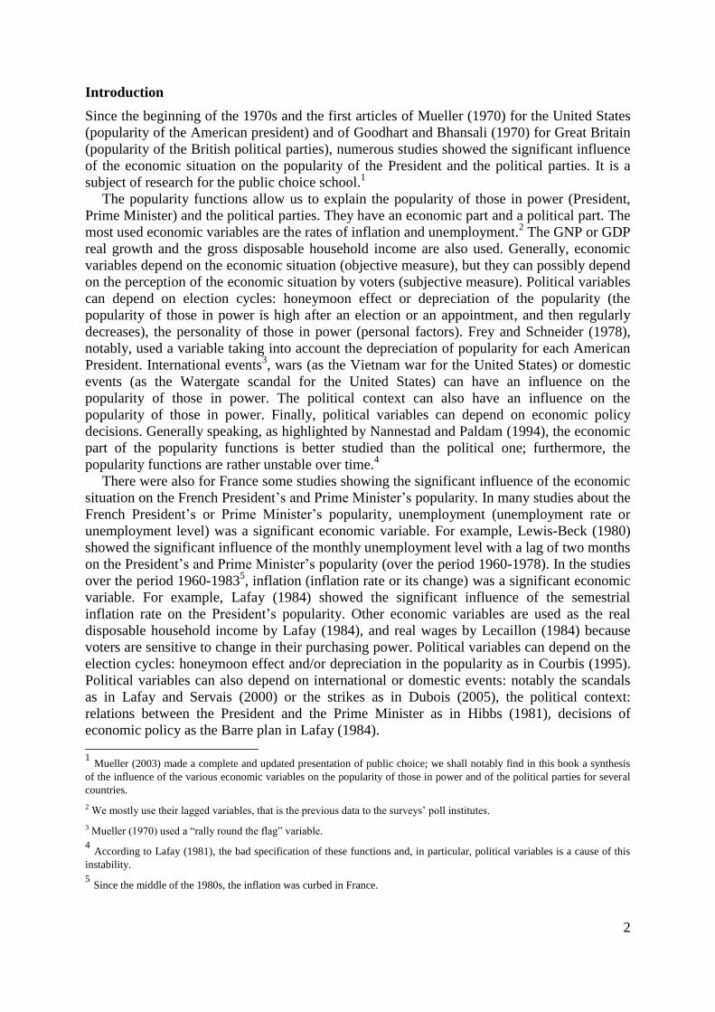
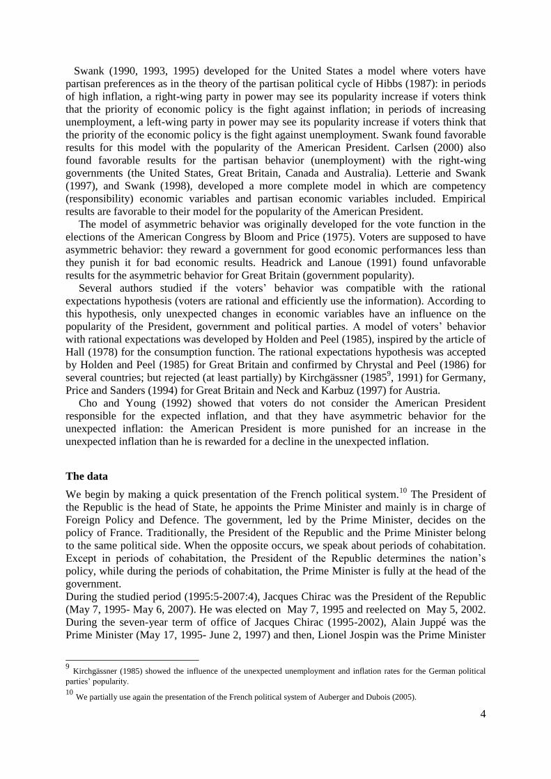
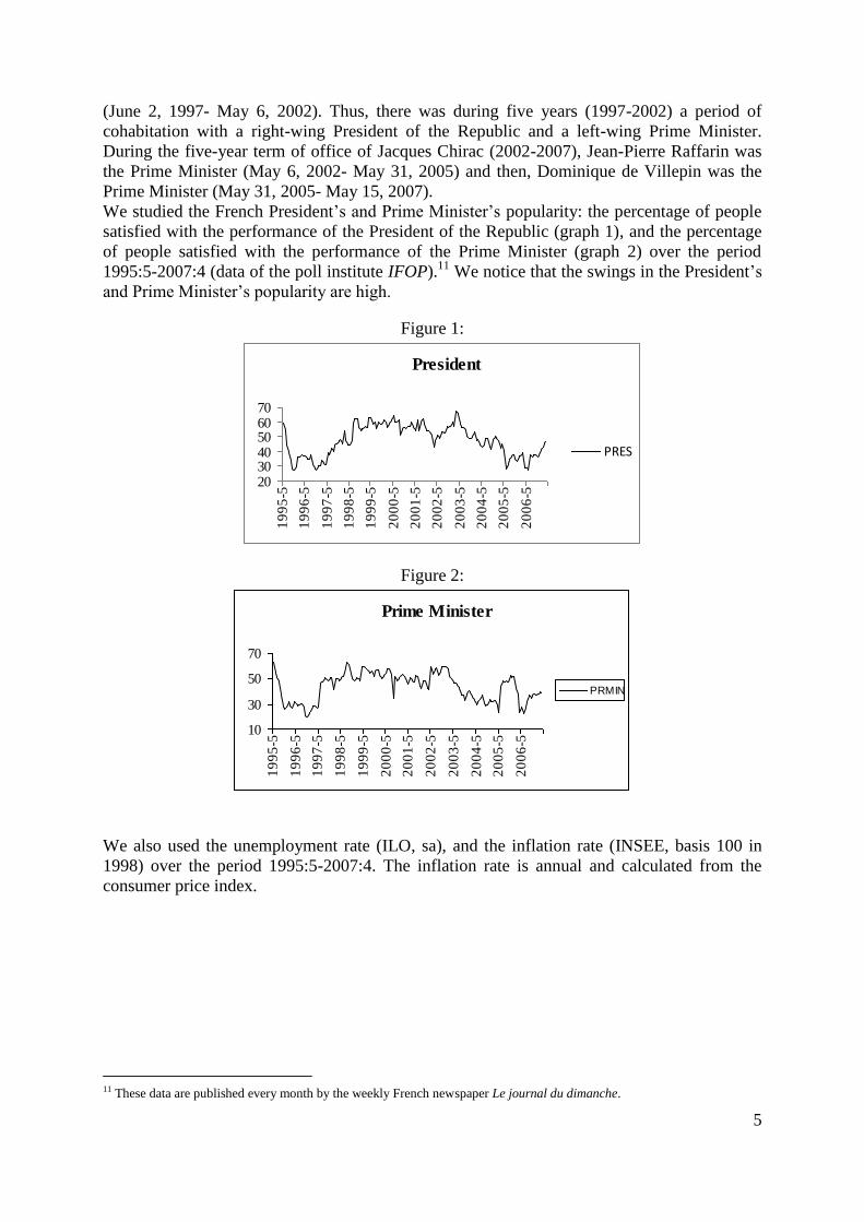
We studied the French President’s and Prime Minister’s popularity: the percentage of people

satisfied with the performance of the President of the Republic (graph 1), and the percentage

of people satisfied with the performance of the Prime Minister (graph 2) over the period

1995:5-2007:4 (data of the poll institute IFOP).11

We notice that the swings in the President’s

and Prime Minister’s popularity are high.

Figure 1:

Figure 2:

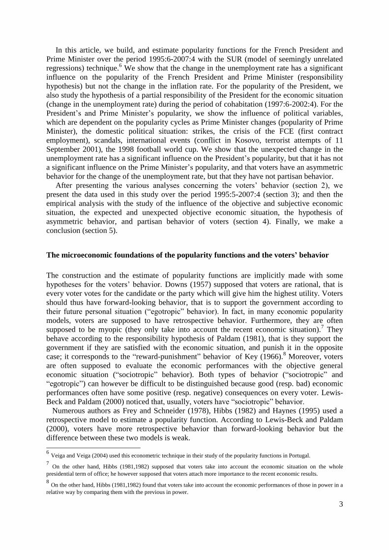
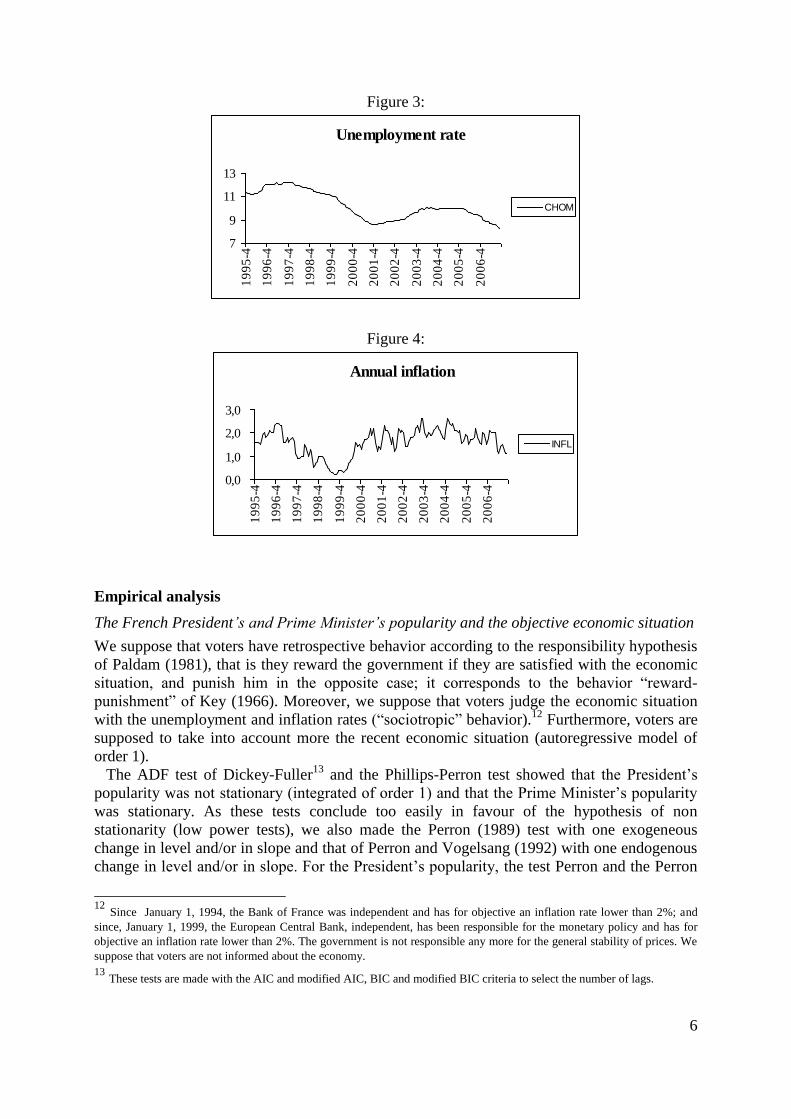
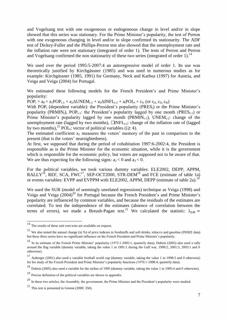
We also used the unemployment rate (ILO, sa), and the inflation rate (INSEE, basis 100 in

1998) over the period 1995:5-2007:4. The inflation rate is annual and calculated from the

consumer price index.

11 These data are published every month by the weekly French newspaper Le journal du dimanche.

President

203040506070

19

95

-5

19

96

-5

19

97

-5

19

98

-5

19

99

-5

20

00

-5

20

01

-5

20

02

-5

20

03

-5

20

04

-5

20

05

-5

20

06

-5

PRES

Prime Minister

10

30

50

70

19

95

-5

19

96

-5

19

97

-5

19

98

-5

19

99

-5

20

00

-5

20

01

-5

20

02

-5

20

03

-5

20

04

-5

20

05

-5

20

06

-5

PRMIN

6

Figure 3:

Figure 4:

Empirical analysis

The French President’s and Prime Minister’s popularity and the objective economic situation

We suppose that voters have retrospective behavior according to the responsibility hypothesis

of Paldam (1981), that is they reward the government if they are satisfied with the economic

situation, and punish him in the opposite case; it corresponds to the behavior “reward-

punishment” of Key (1966). Moreover, we suppose that voters judge the economic situation

with the unemployment and inflation rates (“sociotropic” behavior).12

Furthermore, voters are

supposed to take into account more the recent economic situation (autoregressive model of

order 1).

The ADF test of Dickey-Fuller13

and the Phillips-Perron test showed that the President’s

popularity was not stationary (integrated of order 1) and that the Prime Minister’s popularity

was stationary. As these tests conclude too easily in favour of the hypothesis of non

stationarity (low power tests), we also made the Perron (1989) test with one exogeneous

change in level and/or in slope and that of Perron and Vogelsang (1992) with one endogenous

change in level and/or in slope. For the President’s popularity, the test Perron and the Perron

12

Since January 1, 1994, the Bank of France was independent and has for objective an inflation rate lower than 2%; and

since, January 1, 1999, the European Central Bank, independent, has been responsible for the monetary policy and has for

objective an inflation rate lower than 2%. The government is not responsible any more for the general stability of prices. We

suppose that voters are not informed about the economy. 13

These tests are made with the AIC and modified AIC, BIC and modified BIC criteria to select the number of lags.

Unemployment rate

7

9

11

13

19

95

-4

19

96

-4

19

97

-4

19

98

-4

19

99

-4

20

00

-4

20

01

-4

20

02

-4

20

03

-4

20

04

-4

20

05

-4

20

06

-4

CHOM

Annual inflation

0,0

1,0

2,0

3,0

19

95

-4

19

96

-4

19

97

-4

19

98

-4

19

99

-4

20

00

-4

20

01

-4

20

02

-4

20

03

-4

20

04

-4

20

05

-4

20

06

-4

INFL

7

and Vogelsang test with one exogeneous or endogeneous change in level and/or in slope

showed that this series was stationary. For the Prime Minister’s popularity, the test of Perron

with one exogeneous changing in level and/or in slope confirmed its stationarity. The ADF

test of Dickey-Fuller and the Phillips-Perron test also showed that the unemployment rate and

the inflation rate were not stationary (integrated of order 1). The tests of Perron and Perron

and Vogelsang confirmed the non stationarity of these two series (integrated of order 1).14

We used over the period 1995:5-2007:4 an autoregressive model of order 1. Its use was

theoretically justified by Kirchgässner (1985) and was used in numerous studies as for

example: Kirchgässner (1985, 1991) for Germany, Neck and Karbuz (1997) for Austria, and

Veiga and Veiga (2004) for Portugal.

We estimated these following models for the French President’s and Prime Minister’s

popularity:

POPt = a0 + a1POPt-1 + a2ΔUNEMt-2 + a3ΔINFLt-2 + aiPOLt + ε1t (or ε2t, ε3t, ε4t)

With POPt (dependent variable): the President’s popularity (PRESt) or the Prime Minister’s

popularity (PRMINt), POPt-1: the President’s popularity lagged by one month (PRESt-1) or

Prime Minister’s popularity lagged by one month (PRMINt-1), UNEMt-2: change of the

unemployment rate (lagged by two months), • INFLt-2: change of the inflation rate of (lagged

by two months),15

POLt: vector of political variables (i ).

The estimated coefficient a1 measures the voters’ memory of the past in comparison to the

present (that is the voters’ nearsightedness).

At first, we supposed that during the period of cohabitation 1997:6-2002:4, the President is

responsible as is the Prime Minister for the economic situation, while it is the government

which is responsible for the economic policy, but voters are supposed not to be aware of that.

We are thus expecting for the following signs: a2 < 0 and a3 < 0.

For the political variables, we took various dummy variables: ELE2002, DEPP, APPM,

RALLY16

, REF, SCA, FWC17

, SEP-OCT2000, STR-DEM18

and FCE (estimate of table 1a)

or events variables: EVPP and EVPPM with ELE2002, APPM, DEPP (estimate of table 2a).19

We used the SUR (model of seemingly unrelated regressions) technique as Veiga (1998) and

Veiga and Veiga (2004)20

for Portugal because the French President’s and Prime Minister’s

popularity are influenced by common variables, and because the residuals of the estimates are

correlated. To test the independence of the estimates (absence of correlation between the

terms of errors), we made a Breush-Pagan test.21

We calculated the statistic:

14

The results of these unit root tests are available on request. 15

We also tested the annual change (in %) of price indexes in foodstuffs and soft drinks, tobacco and gasoline (INSEE data)

but these three series have no significant influence on the French President and Prime Minister’s popularity. 16

In its estimate of the French Prime Minister’ popularity (1972:1-2005:1, quarterly data), Dubois (2005) also used a rally

around the flag variable (dummy variable, taking the value 1 in 1991:1 during the Gulf war, 1999:2, 2001:3, 2003:1 and 0

otherwise). 17

Auberger (2001) also used a variable football world cup (dummy variable, taking the value 1 in 1998:3 and 0 otherwise)

for his study of the French President and Prime Minister’s popularity functions (1970:1-1998:4, quarterly data). 18

Dubois (2005) also used a variable for the strikes of 1995 (dummy variable, taking the value 1 in 1995:4 and 0 otherwise). 19

Precise definition of the political variables are shown in appendix. 20

In these two articles, the Assembly, the government, the Prime Minister and the President’s popularity were studied. 21

This test is presented in Greene (2000: 350).

8

∑ ∑

, N is the number of observations (N = 143), M is the number of equations (M

= 2) and is the correlation calculated with the obtained residuals by estimating the models

separately. This statistic follows a chi-square distribution with

degrees of freedom,

and the critical value at the 5% level is: .

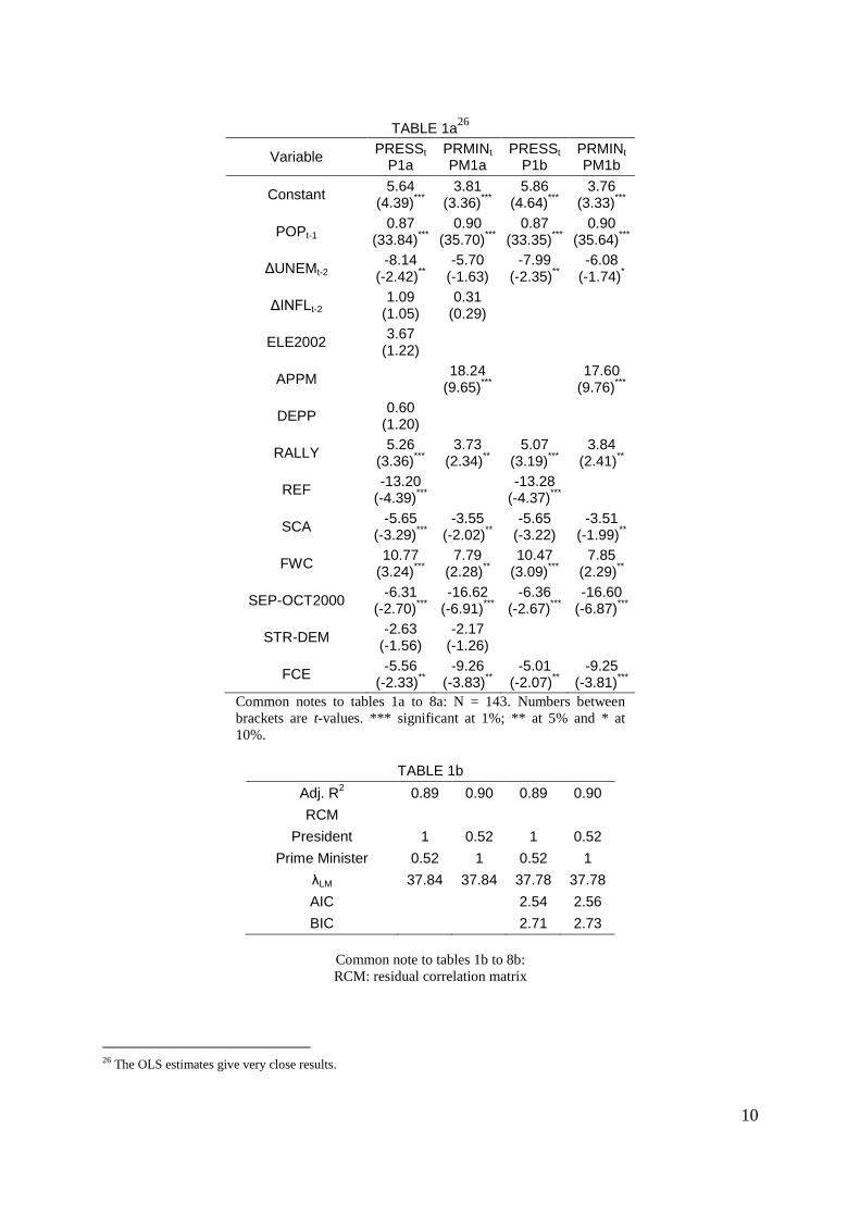
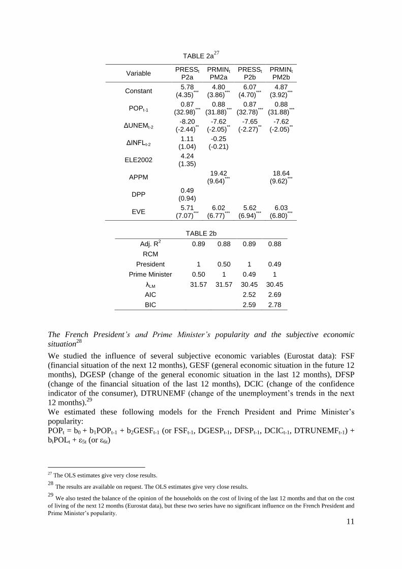
The adjusted R-squared of the estimates of tables 1a and 2a are approximately equal to 0.90

what shows that it accounts for 90% of the variance of variables (PRES and PRMIN). The

coefficient of the UNEMt-2 economic variable has the expected sign, and is significantly

different from 0 at the 5% level for the President’s popularity, and at the 10% level for the

Prime Minister’s popularity: it shows that an increase in the unemployment rate by 0.1% leads

to a decrease in the President’s popularity by about 0.8%, and to a decrease in the Prime

Minister’s popularity by about 0.6% or 0.8%. The coefficient of the UNEMt-2 variable is

higher in absolute value for the President’s popularity than for that of the Prime Minister

(estimates P1b and PM1b, table 1a) or close (estimates P2b and PM2b, table 2a): it is a little

surprising but it can be explained because the Prime Ministers Lionel Jospin, Jean-Pierre

Raffarin and Dominique de Villepin had a honeymoon effect after their appointment, while

Jacques Chirac's weak popularity had completely benefited from the decrease of

unemployment during the cohabitation period (1997:6-2002:4). The coefficient of the

INFLt-2 economic variable is not significantly different from 0 at the 10% level, which shows

that the change of the inflation rate has no significant influence on the President’s and Prime

Minister’s popularity.

The AIC and BIC criteria show that for the President’s popularity, the estimate P2b (with the

EVEP variable) is better than the estimate P1b (with the RALLY, REF, SCA variables) while

they show that for the Prime Minister’s popularity, the estimate PM1b (with the RALLY,

REF, SCA variables) is better than the estimate PM2b (with the EVEPM variable). We notice

that the results of the AIC and BIC criteria are rather close.

The estimates of tables 1a and 2a show that after the Prime Minister’s appointment, the Prime

Minister’s popularity increases from 17.6% or 18.6% (honeymoon effect during the first

month of government with the APPM variable).22,23

We notice that, with the estimates of

tables 1a and 2a, the coefficients of the ELE2002 and DEPP variables are not significantly

different from 0 at the 10% level: it shows that the re-election of the President (Jacques

Chirac) had no significant positive influence on his popularity (no honeymoon effect after its

re-election in May 2002) and that the President (Jacques Chirac) did not have any

depreciation of popularity during his second term of office in comparison with his first term

of office.24,25

These estimates also show the significant positive influence of some

international events (RALLY or EVEP, EVEPM variables: Kosovo war, attempts on

September 11, 2001, the beginning of the military intervention in Afghanistan in October

2001, the French decision against the Iraq war), the football world cup (FWC or EVEP,

22

It means that Alain Juppé did not have a honeymoon effect after his appointment in May 1995 (very fast decrease in his

popularity). 23

We also made estimates with a honeymoon variable for the Prime Minister taking the value 6 during the first month after

its appointment, 5 during the second month, …, 1 during the sixth month and 0 otherwise. The honeymoon variable for the

Prime Minister is significant, but the statistical indicators are a little less satisfactory than with the APPPM variable. 24

It means that Jacques Chirac did not have a honeymoon effect after his election in May 1995 (very fast decline of his

popularity). 25

We also made estimates with a honeymoon variable for the President taking the value 6 during the first month after its

election, 5 during the second month, …, 1 during the sixth month and 0 otherwise. The honeymoon variable for the President

is not significant.

9

EVEPM variables) and the significant negative influence of the rejection of the European

Constitution only on the President’s popularity (variables REF or EVEP) because just after

this rejection, a new Prime Minister was appointed (Dominique de Villepin), and he benefited

then from a honeymoon effect; scandals (variables SCA or EVEP, EVEPM): scandal of the

Prime Minister’s apartment (Alain Juppé) and the Clearstream affair, the gasoline crisis in

September 2000 (SEP-OCT2000 or EVEP, EVEPM variables), the general strikes and the

demonstrations of October and December 1995 against the Juppé plan for the Social Security

and those of May and June 2003 against the pension reform (STR-DEM or EVEP, EVEPM

variables), the FCE (“first contract employment”) crisis in March and April 2006 (FCE or

EVEP, EVEPM variables). The estimates P1b and PM1b allow us to calculate the influence

for the first month of these events individually: about -13.3 % (referendum in 2005 on the

European Constitution), +10.5 % for the football world cup (President’s popularity) and -16.6

% for the gasoline crisis of September 2000 and +16.6 % for the rise which followed in

October 2000 (Prime Minister’s popularity) while the estimates P2b and PM2b give these

events a moderate influence: approximately +6% or -6% for the first month (President’s and

Prime Minister’s popularity).

10

TABLE 1a26

Variable PRESSt

P1a PRMINt

PM1a PRESSt

P1b PRMINt

PM1b

Constant 5.64

(4.39)***

3.81 (3.36)

*** 5.86

(4.64)***

3.76 (3.33)

***

POPt-1 0.87

(33.84)***

0.90 (35.70)

*** 0.87

(33.35)***

0.90 (35.64)

***

ΔUNEMt-2 -8.14

(-2.42)**

-5.70 (-1.63)

-7.99 (-2.35)

** -6.08

(-1.74)*

ΔINFLt-2 1.09

(1.05) 0.31

(0.29)

ELE2002 3.67

(1.22)

APPM

18.24 (9.65)

***

17.60 (9.76)

***

DEPP 0.60

(1.20)

RALLY 5.26

(3.36)***

3.73 (2.34)

** 5.07

(3.19)***

3.84 (2.41)

**

REF -13.20

(-4.39)***

-13.28

(-4.37)***

SCA -5.65

(-3.29)***

-3.55 (-2.02)

** -5.65

(-3.22) -3.51

(-1.99)**

FWC 10.77

(3.24)***

7.79 (2.28)

** 10.47

(3.09)***

7.85 (2.29)

**

SEP-OCT2000 -6.31

(-2.70)***

-16.62 (-6.91)

*** -6.36

(-2.67)***

-16.60 (-6.87)

***

STR-DEM -2.63

(-1.56) -2.17

(-1.26)

FCE -5.56

(-2.33)**

-9.26 (-3.83)

** -5.01

(-2.07)**

-9.25 (-3.81)

***

Common notes to tables 1a to 8a: N = 143. Numbers between

brackets are t-values. *** significant at 1%; ** at 5% and * at

10%.

TABLE 1b

Adj. R2 0.89 0.90 0.89 0.90

RCM

President 1 0.52 1 0.52

Prime Minister 0.52 1 0.52 1

λLM 37.84 37.84 37.78 37.78

AIC

2.54 2.56

BIC 2.71 2.73

Common note to tables 1b to 8b: RCM: residual correlation matrix

26 The OLS estimates give very close results.

11

TABLE 2a27

Variable PRESSt

P2a PRMINt

PM2a PRESSt

P2b PRMINt

PM2b

Constant 5.78

(4.35)***

4.80 (3.86)

*** 6.07

(4.70)***

4.87 (3.92)

***

POPt-1 0.87

(32.98)***

0.88 (31.88)

*** 0.87

(32.78)***

0.88 (31.88)

***

ΔUNEMt-2 -8.20

(-2.44)**

-7.62 (-2.05)

** -7.65

(-2.27)**

-7.62 (-2.05)

**

ΔINFLt-2 1.11

(1.04) -0.25

(-0.21)

ELE2002 4.24

(1.35)

APPM

19.42 (9.64)

***

18.64 (9.62)

***

DPP 0.49

(0.94)

EVE 5.71

(7.07)***

6.02 (6.77)

*** 5.62

(6.94)***

6.03 (6.80)

***

TABLE 2b

Adj. R2 0.89 0.88 0.89 0.88

RCM

President 1 0.50 1 0.49


λLM 31.57 31.57 30.45 30.45

AIC

2.52 2.69

BIC 2.59 2.78

The French President’s and Prime Minister’s popularity and the subjective economic

situation28

We studied the influence of several subjective economic variables (Eurostat data): FSF

(financial situation of the next 12 months), GESF (general economic situation in the future 12

months), DGESP (change of the general economic situation in the last 12 months), DFSP

(change of the financial situation of the last 12 months), DCIC (change of the confidence

indicator of the consumer), DTRUNEMF (change of the unemployment’s trends in the next

12 months).29

We estimated these following models for the French President and Prime Minister’s

popularity:

POPt = b0 + b1POPt-1 + b2GESFt-1 (or FSFt-1, DGESPt-1, DFSPt-1, DCICt-1, DTRUNEMFt-1) +

biPOLt + ε5t (or ε6t)


28 The results are available on request. The OLS estimates give very close results.

29 We also tested the balance of the opinion of the households on the cost of living of the last 12 months and that on the cost

of living of the next 12 months (Eurostat data), but these two series have no significant influence on the French President and

Prime Minister’s popularity.

12

We are expecting for the following signs: b2 > 0 for the GESF, FSF, DGESP, DFSP, DCIC

variables and b2 < 0 for the DTRUNEMF variable.

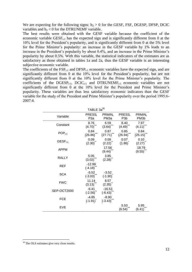
The best results were obtained with the GESF variable because the coefficient of the

economic variable GESFt-1 has the expected sign and is significantly different from 0 at the

10% level for the President’s popularity, and is significantly different from 0 at the 5% level

for the Prime Minister’s popularity: an increase in the GESF variable by 1% leads to an

increase in the President’s popularity by about 0.4%, and an increase in the Prime Minister’s

popularity by about 0.5%. With this variable, the statistical indicators of the estimates are as

satisfactory as those obtained in tables 1a and 2a, thus the GESF variable is an interesting

subjective economic variable.

The coefficients of the FSFt-1 and DFSPt-1 economic variables have the expected sign, and are

significantly different from 0 at the 10% level for the President’s popularity, but are not

significantly different from 0 at the 10% level for the Prime Minister’s popularity. The

coefficients of the DGESPt-1, DCICt-1 and DTRUNEMFt-1 economic variables are not

significantly different from 0 at the 10% level for the President and Prime Minister’s

popularity. These variables are thus less satisfactory economic indicators than the GESF

variable for the study of the President and Prime Minister’s popularity over the period 1995:6-

2007:4.

TABLE 3a30

Variable PRESSt

P3a PRMINt

PM3a PRESSt

P3b PRMINt

PM3b

Constant 8.76

(4.70)***

6.59 (3.64)

*** 8.40

(4.49)***

7.97 (4.11)

***

POPt-1 0.84

(26.86)***

0.87 (27.71)

*** 0.85

(26.94)***

0.84 (25.15)

***

GESFt-1 0.09

(2.30)**

0.09 (2.22)

** 0.07

(1.86)*

0.10 (2.27)

**

APPM

17.56 (9.44)

***

18.79 (9.55)

***

RALLY 5.05

(3.02)***

3.85 (2.28)

**

REF -12.99

(-4.18)***

SCA -5.52

(-3.03)***

-3.52 (-1.90)

*

FWC 11.14

(3.13)***

8.57 (2.35)

**

SEP-OCT2000 -6.41

(-2.56)**

-16.53 (-6.43)

***

FCE -4.85

(-1.91)*

-8.90 (-3.43)

***

EVE 5.53 (6.54)

*** 5.95

(6.41)***


13

TABLE 3b

Adj. R2 0.89 0.90 0.89 0.87

RCM

President 1 0.57 1 0.55


λLM 37.64 37.64 31.54 31.54

AIC 2.54 2.54 2.54 2.69

BIC 2.70 2.71 2.60 2.77

The French President’s and Prime Minister’s popularity and the period of cohabitation

We also estimated these following models for the French President’s and Prime Minister’s

popularity:

POPt = c0 + c1POPt-1 + c2ΔUNEMt-2 + c3COHAB×ΔUNEMt-2 + ciPOLt + ε7t (or ε8t)

With COHAB×UNEM: variable equal to UNEM during the period of cohabitation 1997:6-

2002:4 and to 0 otherwise.

We are expecting for the following signs: c2 < 0 and c3 > 0 with | | < | |, which would

show that during the period of cohabitation (1997:6-2002:4), the President (Jacques Chirac) is

only partially responsible for the economic situation.

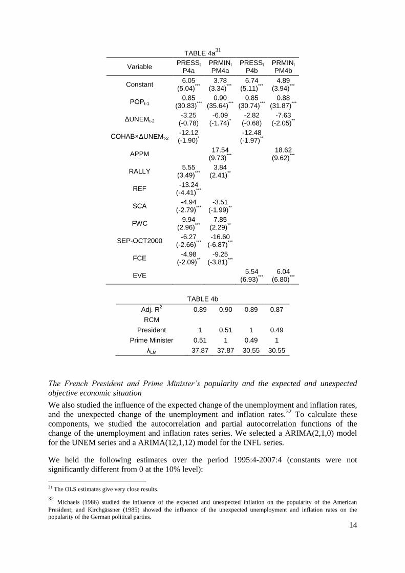
The estimates of table 4a show that the coefficients of the UNEMt-2 and COHAB×UNEMt-2

variables are negative and that of the COHAB×UNEMt-2 variable is higher in absolute value,

which contradicts the partial responsibility hypothesis of the President for the economic

situation during the period of cohabitation. We thus rejected this hypothesis; and we held the

President’s responsibility hypothesis for the economic situation during the period of

cohabitation.

14

TABLE 4a31

Variable PRESSt

P4a PRMINt

PM4a PRESSt

P4b PRMINt

PM4b

Constant 6.05

(5.04)***

3.78 (3.34)

*** 6.74

(5.11)***

4.89 (3.94)

***

POPt-1 0.85

(30.83)***

0.90 (35.64)

*** 0.85

(30.74)***

0.88 (31.87)

***

ΔUNEMt-2 -3.25

(-0.78) -6.09

(-1.74)*

-2.82 (-0.68)

-7.63 (-2.05)

**

COHAB×ΔUNEMt-2 -12.12 (-1.90)

*

-12.48 (-1.97)

**

APPM

17.54 (9.73)

***

18.62 (9.62)

***

RALLY 5.55

(3.49)***

3.84 (2.41)

**

REF -13.24

(-4.41)***

SCA -4.94

(-2.79)***

-3.51 (-1.99)

**

FWC 9.94

(2.96)***

7.85 (2.29)

**

SEP-OCT2000 -6.27

(-2.66)***

-16.60 (-6.87)

***

FCE -4.98

(-2.09)**

-9.25 (-3.81)

***

EVE 5.54 (6.93)

*** 6.04

(6.80)***

TABLE 4b

Adj. R2 0.89 0.90 0.89 0.87

RCM

President 1 0.51 1 0.49


λLM 37.87 37.87 30.55 30.55

The French President and Prime Minister’s popularity and the expected and unexpected

objective economic situation

We also studied the influence of the expected change of the unemployment and inflation rates,

and the unexpected change of the unemployment and inflation rates.32

To calculate these

components, we studied the autocorrelation and partial autocorrelation functions of the

change of the unemployment and inflation rates series. We selected a ARIMA(2,1,0) model

for the UNEM series and a ARIMA(12,1,12) model for the INFL series.

We held the following estimates over the period 1995:4-2007:4 (constants were not

significantly different from 0 at the 10% level):


32 Michaels (1986) studied the influence of the expected and unexpected inflation on the popularity of the American

President; and Kirchgässner (1985) showed the influence of the unexpected unemployment and inflation rates on the

popularity of the German political parties.

15

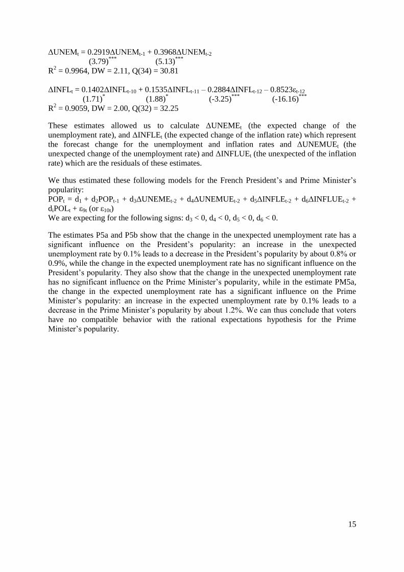
ΔUNEMt = 0.2919ΔUNEMt-1 + 0.3968ΔUNEMt-2

(3.79)***

(5.13)***

R2 = 0.9964, DW = 2.11, Q(34) = 30.81

ΔINFLt = 0.1402ΔINFLt-10 + 0.1535ΔINFLt-11 – 0.2884ΔINFLt-12 – 0.8523εt-12

(1.71)* (1.88)

* (-3.25)

*** (-16.16)

***

R2 = 0.9059, DW = 2.00, Q(32) = 32.25

These estimates allowed us to calculate ΔUNEMEt (the expected change of the

unemployment rate), and ΔINFLEt (the expected change of the inflation rate) which represent

the forecast change for the unemployment and inflation rates and ΔUNEMUEt (the

unexpected change of the unemployment rate) and ΔINFLUEt (the unexpected of the inflation

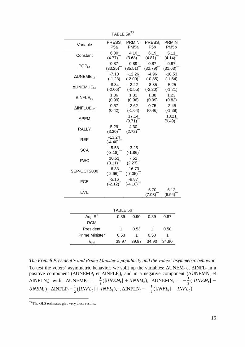
rate) which are the residuals of these estimates. We thus estimated these following models for the French President’s and Prime Minister’s

popularity:

POPt = d1 + d2POPt-1 + d3ΔUNEMEt-2 + d4ΔUNEMUEt-2 + d5ΔINFLEt-2 + d6ΔINFLUEt-2 +

diPOLt + ε9t (or ε10t)

We are expecting for the following signs: d3 < 0, d4 < 0, d5 < 0, d6 < 0.

The estimates P5a and P5b show that the change in the unexpected unemployment rate has a

significant influence on the President’s popularity: an increase in the unexpected

unemployment rate by 0.1% leads to a decrease in the President’s popularity by about 0.8% or

0.9%, while the change in the expected unemployment rate has no significant influence on the

President’s popularity. They also show that the change in the unexpected unemployment rate

has no significant influence on the Prime Minister’s popularity, while in the estimate PM5a,

the change in the expected unemployment rate has a significant influence on the Prime

Minister’s popularity: an increase in the expected unemployment rate by 0.1% leads to a

decrease in the Prime Minister’s popularity by about 1.2%. We can thus conclude that voters

have no compatible behavior with the rational expectations hypothesis for the Prime

Minister’s popularity.

16

TABLE 5a33

Variable PRESSt

P5a PRMINt

PM5a PRESSt

P5b PRMINt

PM5b

Constant 6.00

(4.77)***

4.10 (3.68)

*** 6.19

(4.81)***

5.11 (4.14)

***

POPt-1 0.87

(33.25)***

0.89 (35.51)

*** 0.87

(32.79)***

0.87 (31.63)

***

ΔUNEMEt-2 -7.10

(-1.23) -12.26

(-2.09)**

-4.96 (-0.85)

-10.53 (-1.64)

ΔUNEMUEt-2 -8.34

(-2.06)**

-2.22 (-0.55)

-8.85 (-2.20)

** -5.25

(-1.21)

ΔINFLEt-2 1.36

(0.99) 1.31

(0.96) 1.38

(0.99) 1.23

(0.82)

ΔINFLUEt-2 0.67

(0.42) -2.62

(-1.64) 0.75

(0.46) -2.45

(-1.39)

APPM

17.14 (9.71)

***

18.21 (9.49)

***

RALLY 5.29

(3.30)***

4.30 (2.72)

***

REF -13.24

(-4.40)***

SCA -5.58

(-3.18)***

-3.25 (-1.86)

*

FWC 10.51

(3.11)***

7.52 (2.23)

**

SEP-OCT2000 -6.33

(-2.66)***

-16.73 (-7.05)

***

FCE -5.16

(-2.12)**

-9.87 (-4.10)

***

EVE 5.70 (7.03)

*** 6.12

(6.94)***

TABLE 5b

Adj. R2 0.89 0.90 0.89 0.87

RCM

President 1 0.53 1 0.50


λLM 39.97 39.97 34.90 34.90

The French President’s and Prime Minister’s popularity and the voters’ asymmetric behavior

To test the voters’ asymmetric behavior, we split up the variables: ΔUNEMt et ΔINFLt in a

positive component (ΔUNEMPt et ΔINFLPt), and in a negative component (ΔUNEMNt et

ΔINFLNt) with: ΔUNEMPt =

| | , ΔUNEMNt =

| |

, ΔINFLPt =

| | , , ΔINFLNt =

| |


17

We thus estimated the following models for the French President’s and Prime Minister’s

popularity:

POPt = f1 + f2POPt-1 + f3ΔUNEMPt-2 + f4ΔUNEMNt-2 + f5ΔINFLPt-2 + f6ΔINFLNt-2 + fiPOLt +

ε11t (or ε12t)

We are expecting for the following signs: f3 < 0, f4 < 0, f5 < 0, f6 < 0.

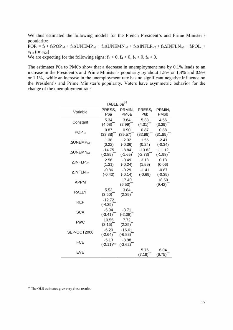
The estimates P6a to PM6b show that a decrease in unemployment rate by 0.1% leads to an

increase in the President’s and Prime Minister’s popularity by about 1.5% or 1.4% and 0.9%

or 1.1%, while an increase in the unemployment rate has no significant negative influence on

the President’s and Prime Minister’s popularity. Voters have asymmetric behavior for the

change of the unemployment rate.

TABLE 6a34

Variable PRESSt

P6a PRMINt PM6a

PRESSt P6b

PRMINt PM6b

Constant 5.34

(4.08)***

3.64 (2.99)

*** 5.38

(4.01)***

4.56 (3.39)

***

POPt-1 0.87

(33.38)***

0.90 (35.57)

*** 0.87

(32.99)***

0.88 (31.85)

***

ΔUNEMPt-2 1.38

(0.22) -2.32

(-0.36) 1.56

(0.24) -2.41

(-0.34)

ΔUNEMNt-2 -14.75

(-2.85)***

-8.84 (-1.65)

* -13.82

(-2.73)***

-11.12 (-1.98)

**

ΔINFLPt-2 2.56

(1.31) -0.49

(-0.24) 3.13

(1.59) 0.13

(0.06)

ΔINFLNt-2 -0.86

(-0.43) -0.29

(-0.14) -1.41

(-0.69) -0.87

(-0.39)

APPM

17.40 (9.53)

***

18.50 (9.42)

***

RALLY 5.53

(3.50)***

3.84 (2.39)

**

REF -12.72

(-4.25)***

SCA -5.94

(-3.41)***

-3.71 (-2.08)

**

FWC 10.55

(3.15)***

7.72 (2.25)

**

SEP-OCT2000 -6.20

(-2.64)***

-16.61 (-6.88)

***

FCE -5.13

(-2.11)** -8.98

(-3.62)***

EVE 5.76 (7.19)

*** 6.04

(6.75)***


18

TABLE 6b

Adj. R2 0.89 0.88 0.89 0.87

RCM

President 1 0.52 1 0.49


λLM 35.89 35.89 33.88 33.88

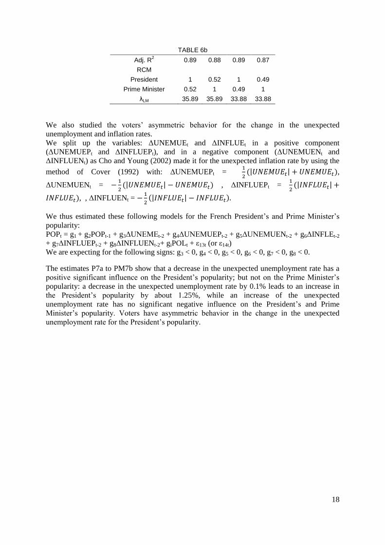
We also studied the voters’ asymmetric behavior for the change in the unexpected

unemployment and inflation rates.

We split up the variables: ΔUNEMUEt and ΔINFLUEt in a positive component

(ΔUNEMUEPt and ΔINFLUEPt), and in a negative component (ΔUNEMUENt and

ΔINFLUENt) as Cho and Young (2002) made it for the unexpected inflation rate by using the

method of Cover (1992) with: ΔUNEMUEPt =

| | ,

ΔUNEMUENt =

| | , ΔINFLUEPt =

| |

, , ΔINFLUENt =

| |

We thus estimated these following models for the French President’s and Prime Minister’s

popularity:

POPt = g1 + g2POPt-1 + g3ΔUNEMEt-2 + g4ΔUNEMUEPt-2 + g5ΔUNEMUENt-2 + g6ΔINFLEt-2

+ g7ΔINFLUEPt-2 + g8ΔINFLUENt-2+ giPOLt + ε13t (or ε14t)

We are expecting for the following signs: g3 < 0, g4 < 0, g5 < 0, g6 < 0, g7 < 0, g8 < 0.

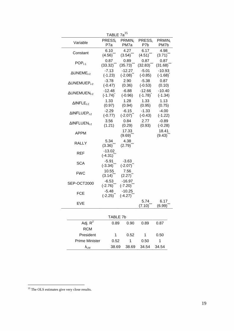
The estimates P7a to PM7b show that a decrease in the unexpected unemployment rate has a

positive significant influence on the President’s popularity; but not on the Prime Minister’s

popularity: a decrease in the unexpected unemployment rate by 0.1% leads to an increase in

the President’s popularity by about 1.25%, while an increase of the unexpected

unemployment rate has no significant negative influence on the President’s and Prime

Minister’s popularity. Voters have asymmetric behavior in the change in the unexpected

unemployment rate for the President’s popularity.

19

TABLE 7a35

Variable PRESSt

P7a PRMINt

PM7a PRESSt

P7b PRMINt

PM7b

Constant 6.10

(4.56)***

4.27 (3.54)

*** 6.17

(4.51)***

4.98 (3.71)

***

POPt-1 0.87

(33.32)***

0.89 (35.73)

*** 0.87

(32.83)***

0.87 (31.68)

***

ΔUNEMEt-2 -7.13

(-1.23) -12.27

(-2.08)**

-5.01 (-0.85)

-10.93 (-1.68)

*

ΔUNEMUEPt-2 -3.78

(-0.47) 2.90

(0.36) -5.38

(-0.53) 0.87

(0.10)

ΔUNEMUENt-2 -12.48 (-1.74)

* -6.88

(-0.96) -12.66 (-1.78)

* -10.40 (-1.34)

ΔINFLEt-2 1.33

(0.97) 1.28

(0.94) 1.33

(0.95) 1.13

(0.75)

ΔINFLUEPt-2 -2.29

(-0.77) -6.15

(-2.07)**

-1.33 (-0.43)

-4.00 (-1.22)

ΔINFLUENt-2 3.56

(1.21) 0.84

(0.29) 2.77

(0.93) -0.89

(-0.28)

APPM

17.33 (9.69)

***

18.41 (9.43)

***

RALLY 5.34

(3.36)***

4.38 (2.79)

***

REF -13.02

(-4.31)***

SCA -5.91

(-3.34)***

-3.63 (-2.07)

**

FWC 10.55

(3.14)***

7.56 (2.27)

**

SEP-OCT2000 -6.53

(-2.76)***

-16.97 (-7.20)

***

FCE -5.48

(-2.25)**

-10.25 (-4.27)

***

EVE 5.74 (7.10)

*** 6.17

(6.99)***

TABLE 7b

Adj. R2 0.89 0.90 0.89 0.87

RCM

President 1 0.52 1 0.50


λLM 38.69 38.69 34.54 34.54


20

The French President’s and Prime Minister’s popularity and the voters’ partisan behavior

We used the partisan model of Swank (1990, 1993, 1995) and we also introduced economic

variables with the responsibility hypothesis as made by Letterie and Swank (1997) and Swank

(1998).

We thus estimated these following models for the French President’s and Prime Minister’s

popularity:

PRESt = h1 + h2PRESt-1 + h3ΔUNEMt-2 + h5ΔINFLt-2 + hiPOLt + ε15t

PRMINt = k1 + k2PRMINt-1 + k3ΔUNEMt-2 + k4(LEFT-(1-LEFT))×ΔUNEMt-2 + k5ΔINFLt-2 +

k6(LEFT-(1-LEFT))×ΔINFLt-2 + kiPOLt + ε16t

We are expecting for the following signs: k3 < 0, k4 > 0 (an increase in the unemployment rate

when the Left is the parliamentary majority leads to an increase in the Prime Minister’s

popularity), k5 < 0, k6 < 0 (an increase in the inflation rate when the Right has the

parliamentary majority leads to an increase in the Prime Minister’s popularity).

The estimates PM8a and PM8b36

show that voters have no partisan behavior for the change in

the unemployment rate because the sign of the variable’s coefficient (LEFT-(1-

LEFT))×ΔUNEM is positive, but it is not significantly different from 0 at the 10% level. We

also notice that the sign of the variable’s coefficient (LEFT-(1-LEFT))×ΔINFL is negative,

but it is significantly different from 0 at the 10% level; thus, voters have no partisan behavior

for the change in the inflation rate.

We also studied the voters’ partisan behavior for the unexpected change in the unemployment

and inflation rates.

We thus estimated the following models for the French President and Prime Minister’s

popularity:

PRESt = l1 + l2PRESt-1 + l3ΔUNEMEt-2 + l4ΔUNEMUEt-2 + l5ΔINFLEt-2 + l6ΔINFLUEt-2 +

liPOLt + ε17t

PRMINt = m1 + m2PRMINt-1 + m3ΔUNEMEt-2 + m4ΔUNEMUEt-2 +

m5(LEFT-(1-LEFT))ΔUNEMUEt-2 + m6ΔINFLEt-2 + m7ΔINFLUEt-2 +

m8(LEFT-(1-LEFT))ΔINFLUEt-2 + miPOLt + ε18t

We are expecting for the following signs: m3 < 0, m4 < 0, m5 < 0, m6 < 0, m7 < 0, m8 > 0.

The estimates PM9a and PM9b37

show that voters have no partisan behavior for the change of

the unexpected unemployment rate because the variable’s coefficient

(LEFT-(1-LEFT))ΔUNEMUE is positive, but it is not significantly different from 0 at the

10% level. Voters have no partisan behavior for the change in the unexpected inflation rate

because the variable’s coefficient (LEFT-(1-LEFT))ΔINFLUE is negative but it is not

significantly different from 0 at the 10% level.

Conclusion

We show that, the change of the unemployment rate has a significant influence

(responsibility hypothesis) for the popularity functions of the French President and Prime

Minister over the period 1995:6-2007:4. On the other hand, the change in the inflation rate has

no significant influence on the French President and Prime Minister’s popularity. The

President is responsible for the economic situation as is the Prime Minister during the period

36 Estimates are available on request.

37 Estimates are available on request.

21

of cohabitation (1997:6-2002:5), and during a usual period of government. We also show that

the future general economic situation has a significant positive influence on the President’s

and Prime Minister’s popularity. Political variables are also studied: we notably show that

every Prime Minister's change has a significant positive influence on the Prime Minister’s

popularity (honeymoon effect), while the re-election of the President (Jacques Chirac) in 2002

had no significant positive influence on the President’s popularity (no honeymoon effect after

his re-election). We also show the significant positive influence of some international events

(Kosovo war, attempts in 11 September 2001, the beginning of the military intervention in

Afghanistan, the French position against the war in Iraq), the football world cup; and the

significant negative influence of the rejection of the European Constitution only on the

President’s popularity, the scandals (apartment of the Prime Minister Alain Juppé and

Clearstream’s affair), the gasoline crisis in September 2000, the general strikes and the

national demonstrations of October and December 1995: Juppé’s Plan for Social Security)

and those of May and June 2003 (pension reform), the crisis for the FCE (“first contract

employment”) of March and April 2006. We show that the change of the unexpected

unemployment rate has a significant influence on the President’s popularity, but that it has no

significant influence on the Prime Minister’s popularity; and that voters have asymmetric

behavior for the change in the unemployment rate, but that they have no partisan behavior.

For future research, we shall also make estimates over a more recent period (since 2007) to

try to explain the President's low popularity (Nicolas Sarkozy) and the Prime Minister’s

higher popularity (François Fillon): the President is very active and present on the domestic

political scene, and also plays the role of the Prime Minister.

22

APPENDIX: POLITICAL VARIABLES

ELECHI02: variable for the President’s re-election of 2002 (Jacques Chirac), taking the

value 1 in 2002:5 and 0 otherwise

DPP: variable for the depreciation of the President’s popularity during the Jacques Chirac's

second term of office, taking the value 1 during the period 2002:5-2007:4 and 0 otherwise

APPM: variable for the appointment of the Prime Minister, taking the value 1 in 1997:6,

2002:5, 2005:6 and 0 otherwise

RALLY: variable around the flag, taking the value 1 in 1999:4 and 1999:5 (Kosovo war), 1 in

2001:9 (attempts on September 11, 2001) and 2001:10 (the beginning of the American

intervention in Afghanistan supported notably by France), 1 in 2003:3 (decision of France

against the American military intervention in Iraq) and 0 otherwise

REF: variable for the referendum on the European Constitution, taking the value 1 in 2005:6

and 0 otherwise

SCA: variable for scandals, taking the value 1 in 1995:6 and 1995:7 (affair of the Prime

Minister’s apartment, Alain Juppé), taking the value 1 in 2006:5 and 2006:6 (Clearstream’s

affair) and 0 otherwise

FWC: variable for the football world cup organized in France and won by the French national

team, taking the value 1 in 1998:7 and 0 otherwise

SEPOCT2000: variable for gasoline crisis in September 2000, taking the value 1 in 1999:9, -1

in 1999:10 and 0 otherwise

STR-DEM: variable for the general strikes and national demonstrations, taking the value 1 in

1995:10 and 1995:12, 1 in 2003:5 and 2003:6 and 0 otherwise

FCE (first contract employment): variable for the FCE (“first contract employment”) crisis,

taking the value 1 in 2006:3, 2006:4 and 0 otherwise

EVE: variable events for the President of the Republic (EVEP) and the Prime Minister

(EVEPM). These two variables are almost identical: taking the value -1 in 1995:6 and 1995:7,

-1 in 1995:10 and 1995:12, 1 in 1998:7, 1 in 1999:5 and 1999:6, 1 in 2000:9 and -1 in

2000:10, 1 in 2001:9 and 2001:10, 1 in 2003:3, -1 in 2003:5 and 2003:6, -1 in 2006:3 and

2006:4, -1 in 2006:5 and 2006:6; moreover, EVEP, taking the value -1 in 2005:6 and 0

otherwise

LEFT, taking the value 1 during the period 1997:6-2002:4 and 0 otherwise

23

References

Auberger, A. (2001). Popularité, cycles et politique économique. Ph.D. dissertation,

University of Paris 2.

Auberger, A. and E. Dubois (2005). The influence of local and national economic conditions

on French legislative elections. Public Choice 125: 363-83.

Bloom, H.S. and D.H. Price (1975). Voter response to short-run economic conditions: the

asymmetric effect of prosperity and recession. American Political Science Review 59(4):

1240-54.

Carlsen, F. (2000). Unemployment, inflation and government popularity - are there partisan

effects ?. Electoral Studies 19(2-3): 141-50.

Cho, S. and G. Young (1992). The asymmetric impact of inflation on presidential approval.

Politics & Policy 30(3): 401-30.

Courbis, R. (1995). La conjoncture économique, la popularité politique et les perspectives

électorales dans la France d’aujourd’hui. Journal de la société de statistique de Paris 136(1):

47-70.

Chrystal, A.K. and D.A. Peel (1986). What can economics learn from political science, and

vice versa ?. American Economic Review 76(2): 62-5.

Cover, J.P. (1992). Asymmetric Effects of Positive and Negative Money-Supply Shocks.

Quarterly Journal of Economics 107(4): 1261-82.

Downs, A., (1957). An Economic Theory of Democracy. Harper and Row, New York.

Dubois, E. (2005). Economie politique et prevision conjoncturelle : construction d’un modèle

macroéconométrique avec prise en compte des facteurs politiques. Ph.D. dissertation,

University of Paris 1.

Frey, B.S. and F. Schneider (1978). An empirical study of politico-economic interaction in the

United States. Review of Economics and Statistics 60: 174-83.

Goodhart, C.A.E. and R.J. Bhansali (1970). Political Economy. Political Studies 18(1): 43-

106.

Greene, W.H. (2003). Econometric Analysis. 5th

edition (international edition), Prentice-Hall.

Hall, R.E. (1978). Stochastic implications of the life-cycle permanent income hypothesis:

theory and evidence. Journal of Political Economy 86(6): 971-87.

Haynes, S.E. (1995). Electoral and partisan cycles between US economic performance and

presidential popularity. Applied Economics 27(1): 95-105.

Headrick, B. and D.J. Lanoue (1991). Attention, Asymmetry, and Government Popularity in

Britain. Western Political Quaterly 44(1): 67-86.

Hibbs, D.A. Jr. (1981). Economics and politics in France: economic performance and mass

political support for Presidents Pompidou and Giscard d’Estaing. European journal of

political research 9: 133-45.

Hibbs, D.A. Jr. (1982). On the demand for economic outcomes: macroeconomic performance

and mass political support in the United States, Great Britain, and Germany. Journal of

Politics 44: 426-62, reprinted in Hibbs, D.A. Jr. (1987). The American political economy:

electoral policy and macroeconomics in contemporary America. Harvard University Press,

Cambridge, MA (199-223).

Hibbs, D.A. Jr. (1987). The political economy of industrial democracies. Cambridge, MA and

London: Harvard University Press.

Holden, K. and D.A. Peel (1985). An alternative approach to explaining political popularity.

Electoral Studies 4(3): 231-39.

Key, V.O. Jr. (1966). The responsible electorate. Cambridge, Harvard University Press.

24

Kirchgässner, G. (1985). Rationality, causality, and the relation between economic conditions

and the popularity of parties. An empirical investigation for the Federal Republic of Germany,

1971-1982. European Economic Review 28: 243-68.

Kirchgässner, G. (1991). Economic conditions and the popularity of West German parties:

before and after the 1982 government change. In Norpoth H., M.S. Lewis-Beck, and J.D.

Lafay (eds.) Economics and politics - The calculus of support. Ann Arbor: The University of

Michigan Press (103-22).

Lafay, J.D. (1981). Situation économétrique et comportements politiques: bilan des études

empiriques et analyse du cas français, communication to annual Congress of the Association

française de sciences économique.

Lafay, J.D. (1984). Political change and stability of the popularity function: the French

general of 1981. Political Behavior 6(4): 333-52, reprinted in Eulau, H. and M.S. Lewis-

Beck, (eds.), 1985, Economic conditions and electoral outcomes: the United States and the

Western Europe, New York: Agathon Press (78-97).

Lafay, J.D. and M. Servais (2000). The impact of political scandals on popularity and votes.

in Lewis-Beck M.S. (ed.), How France Votes, New York: Chatham House (189-205).

Lecaillon, J. 1984. Disparités de revenus et stratégie politique. Revue d'économie politique

94(4) : 433-45.

Letterie, W. and O.H. Swank (1997). Electoral and partisan cycles between US economic

performance and presidential popularity: a comment on Stephen E. Haynes. Applied

Economics 29 (12): 1585-92.

Lewis-Beck, M.S. (1980). Economic conditions and executive popularity: the French

experience. American Journal of Political Science 24: 306-23.

Lewis-Beck, M.S. and M. Paldam (2000). Economic voting: an introduction. Electoral

Studies 19(2-3): 113-21.

Michaels, R. (1986). Reinterpreting the role of inflation in politico-economic models. Public

Choice 48: 113-24. he role of inflation in politico-economic

Mueller, D. (2003). Public Choice III. Cambridge University Press.

Mueller, J. (1970). Presidential popularity from Truman to Johnson. American Political

Science Review 64(1): 18-34.

Nannestad, P. and M. Paldam (1994). The VP-function: a survey of the literature on vote and

popularity functions after 25 years. Public Choice 79: 213-45.

Neck, R. and S. Karbuz (1997). Econometric estimations of popularity functions: a case study

for Austria. Public Choice 91(1): 57-88.

Paldam, M. (1981). A preliminary survey of the theories and findings on vote and popularity

functions. European Journal of Political Research 9(2): 181-189.

Perron, P. (1989). The great crash, the oil price shock, and the unit root hypothesis.

Econometrica 57(6): 1361-1401.

Perron, P. and T.J. Vogelsang (1992). Nonstationarity and level shifts with an application to

purchasing power parity. Journal of Business and Economics Statistics 10(3): 301-20.

Price, S. and D. Sanders (1994). Economic Competence, Rational Expectations and

Government Popularity in Post-war Britain. Manchester School 62(3): 296-312.

Swank, O.H. (1990). Presidential popularity and reputation. de Economist 138(2): 168-180.

Swank, O.H. (1993). Popularity functions based on the partisan theory, Public Choice 75:

339-56.

Swank, O.H. (1995). Rational voters in a partisanship model. Social choice and welfare 12(1):

13-27.

Swank, O.H. (1998). Partisan policies, macroeconomic performance and political support.

Journal of Macroeconomics 30(2): 367-86.

25

Veiga, F.J. and L.G. Veiga (2004). Popularity functions, partisan effects, and support in

Parliament. Economics and Politics 16(1): 101-15.

popularity functions for the french president and … · popularity functions for the french...

Documents