Population Heterogeneity and the Nonprofit Sector in

the United States : Global versus Local Spatial

Approaches

Marie Lebreton, Katia Melnik

To cite this version:

Marie Lebreton, Katia Melnik. Population Heterogeneity and the Nonprofit Sector in theUnited States : Global versus Local Spatial Approaches. 2006. <halshs-00410518>

HAL Id: halshs-00410518

https://halshs.archives-ouvertes.fr/halshs-00410518

Submitted on 21 Aug 2009

HAL is a multi-disciplinary open accessarchive for the deposit and dissemination of sci-entific research documents, whether they are pub-lished or not. The documents may come fromteaching and research institutions in France orabroad, or from public or private research centers.

L’archive ouverte pluridisciplinaire HAL, estdestinee au depot et a la diffusion de documentsscientifiques de niveau recherche, publies ou non,emanant des etablissements d’enseignement et derecherche francais ou etrangers, des laboratoirespublics ou prives.

GREQAM Groupement de Recherche en Economie

Quantitative d'Aix-Marseille - UMR-CNRS 6579 Ecole des Hautes Etudes en Sciences Sociales

Universités d'Aix-Marseille II et III

Document de Travail n° 2006-25

POPULATION HETEROGENEITY AND THE

NONPROFIT SECTOR IN THE UNITED STATES : GLOBAL VERSUS LOCAL

SPATIAL APPROACHES

Marie LEBRETON Katia MELNIK

May 2006

Population Heterogeneity and the

Nonprofit Sector in the United States:

Global versus Local Spatial Approaches

Marie LEBRETON∗and Katia MELNIK†

June 21, 2006

Abstract

In this paper we study the relationship between the relative size ofthe U.S. nonprofit sector and population heterogeneity, at the countylevel, by adopting and extending the model of Alesina, Baquir andEasterly (1999). The relative size of the voluntary sector is assessedas a share of voluntary donations in the total public good providedlocally via public expenditures and private contributions.We demonstrate empirically that the relative size of the nonprofit sec-tor in each county depends not only on its population heterogeneity,but also on its neighbors’ average relative size of the nonprofit sec-tor and average population heterogeneity. Moreover, this relationshipseems to be unstable across counties as the signs and magnitudes ofneighborhood effects vary with geographical location.

JEL classification: C21, D71, H41.

Keywords: Public good, Nonprofit sector, Parameter heterogeneity,Spatial models

1 Introduction

Since the seminal work of Weisbrod (1977, 1986), voluntary organizations arerecognized as alternative mechanisms of private provision of collective-typegoods. Though criticized (e.g. DiMaggio and Anheier, 1990), Weisbrod’sapproach remains the dominant theoretical perspective in the nonprofit field.

∗Marie LEBRETON, GREQAM, Centre de la Vieille Charite, 2 rue de la Charite,13326 Marseille Cedex 2, France. Email: egen us@yahoo.com

†Corresponding author: Katia MELNIK, GREQAM, Vieille Charite, 2 rue de laCharite, 13002 Marseille, France. Email: melnik@ehess.univ−mrs.fr. The authors thanksummer school participants at CORE (Louvain-la-Neuve) for comments and sugges-tions. Further, the authors gratefully acknowledge Jean-Benoıt Zimmermann and AnnePeguin−Feissolle for very helpful suggestions and comments.

1

He pointed out the role of voluntary nonprofit sector as a “major providerof collective-consumption goods which enter positively utility functions of alimited set of persons representing a demand insufficient to organize govern-mental or market provision of excludable goods”. Thus the voluntary sectoris considered as an extra-governmental provider of collective consumptiongoods which represents an alternative for unsatisfied demanders. The unsat-isfied demands arise from the fact that in a majority voting political system,political decisions about provision of local public goods tend to satisfy thedemand of the median voter. Government finances the public provision ofpublic goods by compulsory taxation. In a democratic society with het-erogeneous demand, voters who are not satisfied by the public provision ofcollective good can either move to another jurisdiction or form a voluntaryorganization to supplement the government ’s provision. The broadly quotedWeisbrod’s theory predicts that “the relative size of the voluntary sector ina field [e.g. education or health] can be expected as a function of the hetero-geneity of population demands. Thus, for any given level of governmentallyprovided output, the market share of the voluntary sector in the provisionof collective goods will vary directly with the heterogeneity among individualdemand schedules for these goods”(p.61). While Weisbrod did not proposeany explicit model, he clearly augured that “if two political units differ in thedegree of heterogeneity of their populations, the more homogenous unit will,ceteris paribus, have a lower level of voluntary sector provision of collective-type goods or their private-good substitutes” (idem).In the same perspective, James (1993) presented an empirical cross-countrystudy of educational services provided both by public and nonprofit sectors.She assumed that the relative size of the nonprofit sector in education wasa function of ”excess demand”, ”differentiated demand” for education, cul-tural and income heterogeneity of population, and public policies towardseducation (public educational spending and public subsides to private edu-cation). The excess demand is supposed to stem from people who are un-satisfied by the publicly provided level of education or excluded from publicprovision because of low public spending. The differentiated demand flowsfrom people with preferences for specific features which result from cultural,religious or other affiliations. She studied the relative size of the nonprofitsector in the field of education with the percentage of enrollments in privatenonprofit schools used as proxy. 1 She finds that cultural (and particularlyreligious) heterogeneity of populations is an important determinant of thelarger size of the nonprofit educational sector.Lassen (2006) provides a cross-country study explaining the size of the infor-mal sector by the degree of country’s ethnic heterogeneity. He considers the

1The private sector is considered here as a synonym of the nonprofit one. Accordingto James (1993), in many countries ”nonprofit status is legally required for educationalinstitutions”.

2

informal sector as opposed to the public one and supposes that in ethnicallyheterogenous societies, ethnic communities may constitute an alternative forpublic provision of some public goods. He finds a positive effect of popu-lation ethnic heterogeneity on the size of the informal sector. While usingregional dummy variables, he does not find any significant regional patternin the studied relationship.However, the effects of populations’ heterogeneity on the relative size of vol-untary sector are not straightforward. On the one hand, it is a source ofeconomic and other individual incentives to deliver a public good, which isunder-provided or provided in an unsatisfactory manner by state or mar-ket. On the other hand, previous literature indicated that heterogeneitymay also be a source of inefficiencies in the provision of local public goods(Alesina et al, 1999, Miguel and Gugerty, 2004) and charitable giving in theU.S.A. (Okten and Osili, 2005). In these studies, the economic and socialheterogeneities of population assessed through income inequality and ethnicor religious fractionalization (Alesina et al, 2003) negatively influence theprovision of public goods. Moreover, an empirical study of Alesina and LaFerrara, (2000) on the effects of population heterogeneity on membership ingroups suggests that income and ethnic heterogeneities diminish the propen-sity to participate in social activities (measured as membership in groups),particularly for ”face-to-face” groups, where direct interactions among peo-ple are important. The idea underlying these studies is that heterogeneityin agents’ characteristics may be translated into heterogeneous preferencestowards public good. The question we raise in this paper concerns preciselythe effects of heterogeneity in population characteristics on the portion oflocal public good generated through private donations.

Methodologically, we investigate the effects of population heterogeneityon the relative size of the U.S. nonprofit sector using three different ap-proaches. The first one, the standard linear regression model estimated byOLS assumes that the relationship under study is stationary over space andthat there is no spatial dependence in the observations. As in the empiri-cal papers mentioned above, it is implicitly assumed that observations arespatially independent, i.e. there are no interactions between neighboringcounties.However, spatial dependence may arise when we deal with located observa-tions because of measurement errors for observations or because some unob-served economic and social phenomena present a spatial structure leadingto complex interactions. Therefore, the second estimation approach incor-porates explicitly spatial dependence through the inclusion of the spatiallylagged dependent and independent variables. The maximum likelihood esti-mation of the resulting model called a Spatial Durbin model (SDM) allowsus to demonstrate the existence of geographical spillovers among U.S. coun-ties as the relative size of the nonprofit sector in a county depends not only

3

on the values of its own independent variables, but also on the average val-ues of the dependent and independent variables in the neighboring counties.In order to test the robustness of the SDM results, a Matrix ExponentialSpatial Structure (MESS) model is also estimated. The MESS results sup-port the SDM ones.The possible spatial non stationarity of the relationship under study is alsoignored and results in global modelling. However, the spatial non station-arity of the relationship across counties may result from misspecification inthe model (e.g omitted variables, a wrong functional form) or from intrin-sically different behaviors of local governments. As pointed out by Durlauf(2002), Durlauf and Fafchamps (2003), if the distribution of a given errordepends on its associated geographical area, then a model allowing for para-meter heterogeneity is appropriate to fit the data. In other words, parameterestimates may differ across geographical units (Brock and Durlauf, 2001).Although ignoring this aspect may lead to misleading conclusions concerningstudied relationships between variables, especially in cross-country analysis,most empirical works do not allow for parameter heterogeneity. For instance,Salamon et al (2000) looked at the relationship between the size of nonprofitsector (measured as a percentage of total nonagricultural employment) andthe population’s religious heterogeneity in different countries. Based on theestimations of a linear regression, they concluded that no significant rela-tionship was detected. According to their data, ”...countries with similarlevels of fractionalization, such as Colombia and Ireland, or the Netherlandsand the U.K., vary considerably in the size of their nonprofit sectors” (p.10.) However, does it really make sense to suppose that an increase in ethnicheterogeneity in Latin America and in Europe would have the same effecton the size of the nonprofit sector?To take into account the possible spatial non stationarity, the assumptionof spatial stationarity is alleviated. We use the Spatial Autoregressive LocalEstimate (SALE) model developed by Pace and LeSage (2002) as it accom-modates simultaneously for spatial dependence and parameter heterogene-ity. The SALE results detect spatial variation in the parameter estimatesmeaning that the relationship under study is not stable across counties.The paper is organized as follows. The theoretical foundations are pre-sented in section one. Section two describes the data used for analysis.Section three is devoted to the different econometric approaches adopted inthe paper. Results are displayed in section four. Section five concludes.

2 Theoretical model

To formalize the link between the relative size of the voluntary sector andpopulation heterogeneity, we adopt and extend the model of Alesina et al(1999.)

4

2.1 The model of Alesina, Baqir and Easterly (1999)

Consider a jurisdiction (a county, for instance) of size 1, in which politicaldecisions about the size and the type of local public good g are taken bymajority-vote rule. The individual preferences are written as

Ui = ga(1− li) + c, (1)

with0 < a < 1,

0 ≤ li ≤ 1,

where g is the local public good which can be located on an ”ideological line”[0,1] of individual preferences concerning different types of public good; li isthe distance between the individual i’s preferred public good and the deliv-ered one; c denotes the private consumption. Income is considered as equalfor everybody, and private consumption is equal to disposable revenues:

c = y − t (2)

In (2), y is the pre-tax income and t is the lump-sum tax equal for everyoneby assumption. As the size of population is normalized at 1, the aggregateand per capita variables are the same, so g per capita equals the total sizeof g. Then the public budget constraint is

g = t, (3)

Now individual preferences can be rewritten as follows:

Ui = ga(1− li) + y − g, (4)

Here it is supposed this jurisdiction decides by majority rule first on theamount of taxation and thus on the size of the public good, and second onthe type of the public good.According to the median voter theorem, for anypositive amount of the public good g, the type of public good chosen for theprovision will be the most preferred by the median voter. Thus the optimalsize of the public good is given by the solution of equation (5).

maxUi = ga(1− li) + y − g, (5)

where li is the distance of individual i from the type preferred by the medianvoter. The equation above incorporates the fact that when the decision onthe size of g is taken, the agents know that the type of the publicly providedlocal public good will be the one most preferred by the median voter. Thesolution of (5) gives the individual i’s most preferred size of public good:

g∗i = [a(1− li)]1/(1−a), (6)

5

Now, following Alesina et al (1999) note lm as the median distance from thetype most preferred by the median voter or ”the median distance from themedian”. If the agents know that the type of the public good chosen for thepublic provision will be the one most preferred by the median voter, thenthe amount of public good provided in equilibrium will be given by

g∗ = [a(1− lm)]1/(1−a), (7)

polarization of preferences. voter, Equation (7) implies that in equilibrium,the amount of public good of the type preferred by the median voter is de-creasing in lm.

2.2 Heterogeneity effects on individual utility

On the basis of the model above, it is possible to express the individualutility resulting from g∗ by substituting g∗ in (4).

Ui(g∗) = g∗[1− li

a(1− lm)− 1] + y, (8)

The individual utility drawn from the optimal size and type of public goodg∗ is decreasing with the distance to the median voter li. People with lismaller than lm are relatively close to the type preferred by median voter,while people with li greater than lm are relatively distant, hence less satis-fied by the public provision.The median distance lm can be proxied by some measures of populations’cultural, ethnic, linguistic or religious heterogeneities. Think for instance ofpreferences for education or art that can be strongly related to cultural orethnic backgrounds.According to this model, when an important fraction of population is at agreat distance from the median voter, hence the median distance from themedian voter preferred type is large, and the type of public good is far fromcorresponding to the preferences of a large share of population. In this casethis population would prefer to contribute less to this public good and tokeep taxes low. On the other hand, this category of population would devotemore resources to private consumption. The wealthiest people can replacecollective-type good by its private substitutes. Moreover, in some jurisdic-tions with heterogeneous population, public resources may be directed tosome specific groups of population via some preferential treatments or ”pa-tronage” (Alesina et al, 1999).In this paper we assume that people who are unsatisfied by the public pro-vision of collective-type goods may create voluntary organizations or con-tribute to them in order to provide collective-type goods or services thatcorrespond better to their preferences and needs (Weisbrod, 1986.)

6

2.3 The case with voluntary contributions

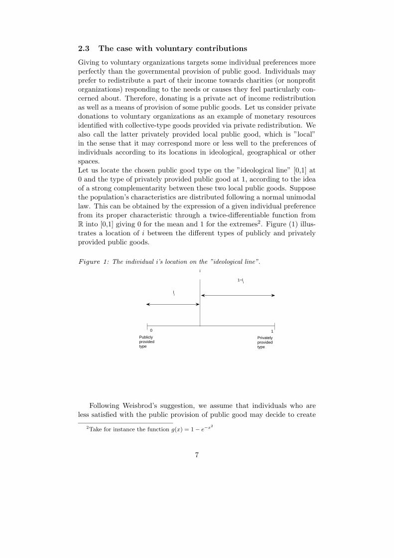
Giving to voluntary organizations targets some individual preferences moreperfectly than the governmental provision of public good. Individuals mayprefer to redistribute a part of their income towards charities (or nonprofitorganizations) responding to the needs or causes they feel particularly con-cerned about. Therefore, donating is a private act of income redistributionas well as a means of provision of some public goods. Let us consider privatedonations to voluntary organizations as an example of monetary resourcesidentified with collective-type goods provided via private redistribution. Wealso call the latter privately provided local public good, which is ”local”in the sense that it may correspond more or less well to the preferences ofindividuals according to its locations in ideological, geographical or otherspaces.Let us locate the chosen public good type on the ”ideological line” [0,1] at0 and the type of privately provided public good at 1, according to the ideaof a strong complementarity between these two local public goods. Supposethe population’s characteristics are distributed following a normal unimodallaw. This can be obtained by the expression of a given individual preferencefrom its proper characteristic through a twice-differentiable function fromR into [0,1] giving 0 for the mean and 1 for the extremes2. Figure (1) illus-trates a location of i between the different types of publicly and privatelyprovided public goods.

Figure 1: The individual i’s location on the ”ideological line”.

li

1−li

0 1

i

Publiclyprovidedtype

Privatelyprovidedtype

Following Weisbrod’s suggestion, we assume that individuals who areless satisfied with the public provision of public good may decide to create

2Take for instance the function g(x) = 1− e−x2

7

or to contribute to a nonprofit. We incorporate this idea into the model byintroducing voluntary contributions into the basic expression of individualutility. Incorporating the voluntary contributions into equation (4) yieldsequation (9):

Ui = g∗a(1− li) + dbli + y − g∗ − di(1− γ), (9)

0 < b < 1,

where di is the individual i’s contribution to the differentiated publicgood, b is the parameter of technology of the privately provided local publicgood and γ is the marginal tax rate. As equation (9) shows, the model de-scribes the context of a jurisdiction, where voluntary donations are deducedfrom imposable revenues.

d =∑

i

di, (10)

Equation (9) assumes that technologies a and b of publicly and privatelyprovided local public goods are independent and may differ.If the type and the amount of public good are the most preferred by themedian voter, the individual’s preferred amount of contribution is given bythe solution of:

maxUi = g∗a(1− li) + db li + y − g∗ − di(1− γ), (11)

where g∗ is given by (7). The solution of (11) for di is

d∗i = [1− γ

bli]

1b−1 , (12)

Now the amount of giving may be defined by

d∗ = [1− γ

blm]

1b−1 , (13)

From equation (13) it follows that the equilibrium amount of giving thatwe associate with the differentiated public good is increasing in lm, the me-dian distance from the type preferred by the median voter.The total supply of public good can be written as the sum of publicly andprivately provided public goods G = g + d, where d is the differentiatedpublic good corresponding to the part of expenditures targeting the pref-erences of those who donate better, and g is the part of pure public goodcorresponding to the median voter’s most preferred type and not or veryimperfectly to the demand of the people whose preferences are located farfrom the median voter’s preferences.As Figure (2) shows, the increasing heterogeneity in population’s character-istics measured by lm leads to the raise of the share of privately provided

8

public good in total public good G (noted Rd = d/G and represented by thecontinuous line), and to the decrease of the portion of its public provision(noted Rg = g/G and represented by the dropped line).

Figure 2: Rg (dotted line) and Rd (continuous line) as functions of lm, when a=b=0.5 and γ = 0.2

0

0.2

0.4

0.6

0.8

1

0.2 0.4 0.6 0.8 1

l_m

The rest of the paper provides empirical evidences of the relationshipbetween the relative size of privately provided public good and population’sheterogeneity.

3 The data

The following proposal from an advertisement well illustrates why voluntarycontributions can be considered as a means of supporting cause an individualfeels concerned about: ”When choosing a charity, it is important to decidewhat is most important to you. Most likely, it will be something that haspersonally affected you. For example, consider your Alma Mater, medicalresearch for a disease that a loved one has endured, the training fund for anathlete you admire, or a local community initiative”.In the United States the voluntary sector is represented by two main typesof nonprofit organizations. The first one embodies the organizations regis-tered in section 501(c)3 of the Internal Revenue Code (this category includescultural organizations, foundations, nonprofit schools and universities, day-care centers, charities, and community improvement organizations amongothers.) These organizations are tax exempt, and they can receive tax-deductible charitable donations from individuals, but cannot engage in anypolitical or commercial activities. The second type is represented by theorganizations falling under the smaller 501(c)4 category such as some so-cial welfare organizations, organizations performing lobbying activities onbehalf of specific issues, social clubs and others. Generally, contributionsto this type of nonprofit are not tax-deductible, except for some volun-teer fire companies and similar organizations, as well as some war veteran’sorganizations. One cannot deduct his or her donations to labor unions, po-litical candidates, social clubs, homeowner associations, most of the foreign

9

charities, and organizations performing social activities for the pleasure orrecreation of members.In the U.S. only itemized donations reduce taxable income.3 The tax sav-ing from the act of giving usually equals the amount of deduction (which isnormally the total contributed except in some cases) times the marginal taxrate, namely the top rate for the person’s income level. Giving to federal,state, and local government is also tax-deducible if the contribution is forpublic purposes. However, voluntary organizations are more likely to attractprivate monetary and labor donations than governments (Rose-Ackerman,1996.) According to the Internal Revenue Service (IRS), in 1998 the directcontributions represented more than 50 percent of total contributions, giftsand grants received by 501(c)3 organizations. Americans gave 160 billiondollars to charities in 1998, and donations rose up to 212 billion in 2001.According to IRS, in 1999 about 35.5 million taxpayers made deductiblecharitable contributions totaling nearly 125.8 billion dollars. Contributionsfrom individuals account for more than 75 percent and about 82 percent oftotal giving is itemized for federal income tax returns.4 The data concern-ing the giving are drawn from the National Center for Charitable Statistics.They indicate the amount of total itemized households’ contributions byU.S. county. Counties seem to represent a relevant level of analysis as theydeal with provision of a large fraction of local public goods. They supportthe provision of local public goods in the fields of public welfare, health andhospitals, environment and housing (parks, recreation, community develop-ment) among others. The provision of local public goods is financed by localtaxes (e.g. property tax, 23,3 percent of general revenue), intergovernmentaltransfers (35.5 percent in 1996-97, coming mostly from states), and charges.According to the U.S. Census Bureau,5 in 1996-97, the U.S. counties’ expen-ditures on public welfare, educational services, hospitals, health, and parksand recreation equaled respectively 13.5 percent, 13.2 percent, 9.8 percent,7.3 percent, and 2 percent of total expenditures.For the analysis provided below, it is important to mention that U.S. coun-ties kept their borders constant over years. The dependent variable whichis supposed to indicate the share of impure public good in total public goodis constituted as follows: Y = Rd = d

d+g , where d is the amount of totalhouseholds’ contributions in each county reported in 1998, g is the amountof public expenditures in each county in 1996-97 which comes from the U.S.Census Bureau, 1997 Census of Governments.As we are testing the local effects of population heterogeneity on the relativesize of the voluntary sector, our main explanatory variable we are interestedin is the index measuring population heterogeneity. We employ the broadly-

3The donations are deduced from the federal personal income tax.4In this study we do not take into account the non-itemized charitable contributions.5Source:http://www.census.gov/govs/estimate/97countysummary.html

10

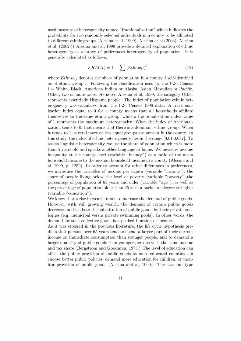
used measure of heterogeneity named ”fractionalization” which indicates theprobability for two randomly selected individuals in a county to be affiliatedto different ethnic groups (Alesina et al (1999), Alesina et al (2003), Alesinaet al, (2002.)) Alesina and al, 1999 provide a detailed explanation of ethnicheterogeneity as a proxy of preferences heterogeneity of population. It isgenerally calculated as follows:

FRACTj = 1−∑

(Ethnicij)2, (12)

where Ethnicij denotes the share of population in a county j self-identifiedas of ethnic group i. Following the classification used by the U.S. Censusi = White, Black, American Indian or Alaska, Asian, Hawaiian or Pacific,Other, two or more races. As noted Alesina et al, 1999, the category Otherrepresents essentially Hispanic people. The index of population ethnic het-erogeneity was calculated from the U.S. Census 1998 data. A fractional-ization index equal to 0 for a county means that all households affiliatethemselves to the same ethnic group, while a fractionalization index valueof 1 represents the maximum heterogeneity. When the index of fractional-ization tends to 0, that means that there is a dominant ethnic group. Whenit tends to 1, several more or less equal groups are present in the county. Inthis study, the index of ethnic heterogeneity lies in the range [0.01 0.687]. Toassess linguistic heterogeneity, we use the share of population which is morethan 5 years old and speaks another language at home. We measure incomeinequality at the county level (variable ”incineg”) as a ratio of the meanhousehold income to the median household income in a county (Alesina andal, 1999, p. 1259). In order to account for other differences in preferences,we introduce the variables of income per capita (variable ”income”), theshare of people living below the level of poverty (variable ”poverty”),thepercentage of population of 65 years and older (variable ”age”), as well asthe percentage of population older than 25 with a bachelors degree or higher(variable ”education”).We know that a rise in wealth tends to increase the demand of public goods.However, with still growing wealth, the demand of certain public goodsdecreases and leads to the substitution of public goods by their private ana-logues (e.g. municipal versus private swimming pools). In other words, thedemand for such collective goods is a peaked function of income.As it was stressed in the previous literature, the life cycle hypothesis pre-dicts that persons over 65 years tend to spend a larger part of their currentincome on immediate consumption than younger people, and to demand alarger quantity of public goods than younger persons with the same incomeand tax share (Bergstrom and Goodman, 1973.) The level of education canaffect the public provision of public goods as more educated counties canchoose better public policies, demand more education for children, or mon-itor provision of public goods (Alesina and al, 1999.) The size and type

11

of population may affect the share of giving in the total public expendi-tures in different manners. For example, large urban jurisdictions are oftenconsidered as suffering from inefficiencies in the provision of public goodsand as more unwieldy than small ones. Therefore, in some jurisdictionspeople may contribute relatively more to nonprofits in the amount of localexpenditures. Moreover, in larger urban jurisdictions the amount of givingmay be positively affected by the greater number of organizations askingfor voluntary contributions. On the other hand, as jurisdictions with smallpopulation can exert more social control, one can speculate that voluntaryincome redistribution could be higher in smaller jurisdictions. We assess thetype of population through the log of urban population in each county. Thesize of population is assessed through the log of population of each countyreported in the US Census 1997. The set of the explanatory variables usedin the model is written as :X = [ι, frac, incineg, otherlanguage, log population, log urban population, poverty,education, age, income per capita], with ι denoting a vector of constant term6.The location of the 3111 counties is determined using the 1990 census in-formation on latitude and longitude. 48033, We have decided to excludefrom the analysis, observations related to the District of Columbia (zip code11001) because of its special status. Alaska and Hawaii have also been ex-cluded from the analysis as they do not share a common border with othercounties. Associated with the initial 23 missing values in the dataset, weget a sample of 3083 observations.

4 The spatial econometric approach

4.1 Global models with fixed spatial weight matrix

4.1.1 Assuming homoscedastic errors

When observations are geographical units as countries, spatial dependenceand heterogeneity may arise among observations. Spatial dependence is de-fined as the lack of independence between observations over space (Anselin,1988). For instance, positive spatial dependence occurs when similar loca-tions in space exhibit similar values which leads to apparent clusters in space.To accommodate spatial autocorrelation in the disturbances, the spatial er-ror model (SEM) has been developed. For a dataset with n geographical

6Collinearity had not been detected in the data according to the BKW (1980) diag-nostics.

12

units, it is written as

y = Xβ + ε

ε = λWε + u

u ∼ N(0, σ2In)(14)

where y is the (n × 1) vector of dependent variable, X is the (n × (k + 1))matrix of explanatory variables including a constant term, W is the (n×n)matrix of spatial weights used to define the structure of the correlations be-tween the disturbances and λ, the parameter of interest denotes the strengthof this spatial dependence.The weighting scheme used to design W is usually based on contiguity be-tween counties. In each row of W, A positive value is assigned to countiesthat are close ’enough’ to county i to be considered as its neighbors and anull value otherwise, with i = 1, . . . , n. The diagonal of this matrix containszero element as a county cannot be used to predict itself.The SEM log-likelihood function is given in (15).

lnL = −(n/2)ln(2π)− (n/2)lnσ2 + ln | I − λW |−(1/2σ2)(y −Xβ)′(I − λW )′(I − λW )(y −Xβ).

(15)

The first order conditions give the generalized least squares estimate for βand σ2, conditional on λ:

βML = [(X − λWX)′(X − λWX)]−1(X − λWX)′(y − λWy). (16)

σ2ML = (e− λWe)′(e− λWe)/n, (17)

with e = y −XβML. Introducing (16) and (17) in (15) leads to the concen-trated log-likelihood function for the SEM model.

lnLC = C − (n/2)ln[(e′(I − λW )′(I − λW )e)/n] + ln | I − λW | . (18)

Pre-multiplying (14) by (I − λW ) leads to (19).

y = λWy + Xβ − λWXβ + u. (19)

This model may be written as what is known as the spatial Durbin model(see Anselin L. and Bera A.K.(1998)) given in (20) if the restriction −λβ = γis imposed in (19).

y = λWy + Xβ + WXγ + u (20)

where X denotes the matrix of independent variables without the constantterm (i.e. each row of X is defined as xi = [1, xi]). In the spatial Durbin

13

model (SDM), the dependent variable is explained firstly by a set of inde-pendent variables, secondly by the average of the dependent variable (Wy)in neighboring counties and thirdly by the average of the independent vari-ables in neighboring counties (WX). The concentrated log-likelihood func-tion for the SDM model is formulated in (21) with e0 = y−Xβ−WXγ ande1 = Wy −Xβ −WXγ.

ln(L) = C − ln | I − λW | −(N/2)ln(e′0e0 − 2λe′1e0 + λ2e′1e1). (21)

The Burridge common factor allows us to test this restriction. If this con-straint cannot be rejected, a model with spatial dependence in the distur-bances is estimated, otherwise a SDM is estimated.However as United States counties do not have the same size, heteroscedas-ticity in the error term may occur. Moreover as noted by LeSage (1997)”enclave effects”7 may lead to fat tailed errors or t distributed errors. ThusLeSage proposed to estimate global spatial models with the Bayesian methodin order to correct this failure.

4.1.2 Assuming heteroscedastic errors

LeSage J.P (1997) proposed to introduce an additional fixed but unknownparameter noted r in the global spatial model in order to accommodate out-liers and observations with large variances. For instance, the heteroscedasticspatial Durbin model may be written as:

y = λWy + Xβ + WXγ + ε

ε ∼ N(0, σ2V )V = diag(v1, v2, . . . , vn)

(22)

A chi-squared prior distribution for the terms in V is suggested by LeSageπ(r/vi) = IIDχ2(r) as it reduces to introducing a single parameter noted r;a normal-gamma conjugate prior for β and γ, and σ2 when the sample sizeis large which may be formulated as follows for θ = [β γ]: π(θ) ∼ N(c, T ),with c and T taking large values, and π(1/σ2) ∼ Γ(d, v). Finally a uniformprior for λ is set as π(λ) = U [0, 1].

4.2 Global models with flexible spatial weight matrix

Note that not only the estimation and inference results presented in thepreceding section are conditional on the specification of the spatial weightmatrix, but also this specification takes place before estimating the model

7When the relationship under study is different in a particular set of counties comparedto the entire territory under study, this is known as ”enclave effects”.

14

whose aim is to detect and estimate the spatial interactions designed in W.LeSage and Pace (2000a) proposed a Matrix Exponential Spatial Structuremodel in which a flexible form for the spatial weight matrix is allowed andis an integral part of the spatial model estimation. They also developed aversion of the MESS model (2000b) robust to heteroscedastic disturbancesand outliers in which the spatial weight matrix will be a linear combinationof individual nearest neighbor matrices with declining coefficients as we movefrom the first nearest neighbors to the second and so on. This flexible weightmatrix takes the form:

W =q∑

i=1

(ρiNi∑qi=1 ρi

)(23)

where Ni represents the spatial matrix associated with the ith nearest neigh-bors in space with i = 1, . . . , q. q is the maximum number of nearest neigh-bors to take into account, these can be first order neighbors (i.e. directneighbors), second order neighbors (neighbors of neighbors) or higher orderneighbors of observations. ρ is the decay parameter which is specific to eachindividual matrix N.The Bayesian MESS model given in (25) relies on the spatial weight matrixexponential transformation of the dependent variable specified in (26)

Sy = Zθ + ε,

ε ∼ N(0, σ2In) (24)(25)

with S the (n× n) positive, definite matrix:

S = eαW (26)

with W defined in (23)and Z = [XWX . . . W l−1X], the matrix of explana-tory variables with independent variables noted X (excluding a constantterm) and lagged independent variables up to order (l-1). LeSage and Pace(2000) recommended to set l = 7 to ensure the convergence in the Taylorseries expansion. Note that the ’traditional ’spatial dependence parameter,noted before λ can be recovered as λ = 1− eα.Robust estimates to non constant variance in the error terms can be ob-tained through a Bayesian heteroscedastic model with the same prior forθ, σ2, vi as in the Bayesian heteroscedastic spatial Durbin model. Non in-formative priors on α, ρ and q i.e. the parameters entering the spatialweight matrix are assigned using uniform distributions. More particularly,π(α) = U [−∞, 0], π(ρ) = U(0, 1) and π(q) = UD[1, qmax].

4.3 Local model: SALE

When we deal with spatial dataset, the hypothesis of spatial stationaritydefined as the stability over space of the relationship under study (Anselin,

15

1988) is often not met. In this case, local models like the nonparametriclocally weighted regression (LWR) model developed by McMillen (1996) aremore appropriate than global ones as they allow for parameter heterogeneity.However the widely used LWR method gives results that are conditional on asingle value of the bandwidth appearing in the weighting function. Chang-ing this value produces different estimated values for the parameters andconsequently different conclusions regarding the stationarity of the relation-ship under study. Moreover the LWR model has been constructed in sucha way that the smaller is the sub-sample size, the less frequently the spa-tial dependence is likely to occur. Thus the LWR parameter estimates canbe used to test the variability over space of the relationship under study.However, a locally weighted regression on a smaller sub-sample size leads tomore volatile parameter estimates which may question the significance of thedetected regional patterns in the parameter estimates. Furthermore, as theabsence of spatial dependence in the LWR residuals cannot be guaranteedin small sub-sample size, estimating a local model with a spatially laggeddependent variable as additional explanatory variable and then testing thesignificance of the spatial dependence parameter seems appropriate. Thus todeal simultaneously with spatial dependence and parameter heterogeneity,Pace and LeSage (2002) propose a Spatial Autoregressive Local Estimation(SALE). It takes the following form:

M(i)y = M(i)Wyλi + M(i)Xβi + M(i)WXγi + M(i)ε. (27)

The vectors y and ε, the matrices X and W are the same as those previouslydefined with (14). M is a (n × n) diagonal matrix in which a value of oneis assigned to the m-nearest neighbors to observation i and a zero value forthe others. M allows to extract a sub-sample on which the regressions areconducted. M(i)Wy is the spatially lagged dependent variable and its as-sociated parameter, noted λi, measures the extent to which the dependentvariable in i, noted M(i)y may be explained by the average of the ones ofits nearest neighbors in space, M(i)Wy. Similarly, γi denotes the effect ofthe average of the independent variables in the neighborhood of i on yi. Aspointed out by Pace and LeSage (2002), the inclusion of the spatially laggeddependent variable in the model may firstly solve the spatial dependenceproblem arising from large sub-sample size and secondly may decrease thesensitivity of the parameter estimates to the bandwidth resulting in morestable estimates.Contrary to the LWR model, the SALE model may be estimated for anysub-sample size, simply by modifying the matrix M. This provides a wayto investigate the occurrence of spatial dependence as the number of neigh-bors is no longer constrained. In other words, this method enable us tosee how the spatial dependence parameter changes with the sub-sample sizefrom small to full sample i.e. from SALE (respectively LSDM) estimates(reflecting parameter heterogeneity) to SAR (respectively SDM). estimates

16

(reflecting parameter homogeneity).Even if both methods seem similar, they are methodologically different. Inthe LWR framework, the weighting scheme places a uniformity condition onthe parameter of spatially neighboring observations. This is not the case inthe the SALE method. Analyzing the beta convergence parameter estimatesfor each observation of the sample, LeSage and LeGallo (2003) investigatethe empirical supporting existence of the local convergence concept in Eu-rope.The SALE estimates are the ones which maximize the following profile like-lihood function (see Anselin, 1988, Pace and Barry, 1997):

lnL(λ) = C + ln | I − λW | −(n/2)ln(SSE(λ)), (28)

where C denotes a constant and SSE(λ), the sum of squared errors.

5 The results

5.1 Global aspatial and spatial models

A linear regression model is estimated with ordinary least squares. Table1 gives the estimation and inferences results of the standard linear regres-sion model. All the coefficients are significant on at least 5 %. The OLSadjusted measure of fit is 0.3107. Values in brackets are the t-probabilitycoming from White (1980) variance matrix robust to heteroscedasticity. Thepositive and significant coefficient of fractionalization is consistent with thetheoretical model. Parameter associated with income inequality has a weaknegative effect, as well as the share of people in a county speaking otherlanguage. The log of urban population has the strongest influence on therelative size of voluntary sector. As expected, age has a negative but smallsignificant effect, while the size of county assessed through the log of pop-ulation demonstrates a small positive effect. Finally, income per capita hasthe smallest positive global effect.The OLS errors are non normally distributed according to the Jarque-Beratest. They are also heteroscedastic as the null hypothesis of the Koenker(1981) test robust to normal errors can be rejected at the significant levelof 5%. Moreover, two tests against unspecified alternative for the spatialdependence process have been carried out. The spatial dependence in thedisturbances is tested using a contiguity matrix found by Delaunay triangu-lation. The Moran I-statistic, adapted to the OLS residuals by Cliff and Ord(1981) indicates spatial dependence in the OLS residuals. But, according toFingleton (1999), this test statistic may detect not only spatial dependencebut also spatial non stationarity. It is also not reliable when heteroscedas-ticity occurs. Thus in order to evaluate the significance of both effects, testsagainst specified alternatives have been realized. They have been noted

17

LMLAG and LMERR. The decision rule elaborated by Anselin and Florax(1995) enables us to choose a spatial error specification as the RLMERRstatistic is significant whereas the RLMLAG is not 8. Bidirectional testshave also been done. Clearly, spatial dependence and heteroscedasticity arethe joint source of misspecification in the model. Thus a model with spatialdependence in the error terms has been estimated by maximum likelihood.The estimated results of the SEM model are given in the second columnof Table 1. The SEM model produces a positive and significant spatial au-tocorrelation parameter. The introduction of the latter rises the adjustedmeasure of fit by 50 percent. According to he LMLAG* test introducinga spatially lagged dependent variable as additional explanatory variable tothe SEM model is not necessary. However, the Burridge common factortest indicates that the spatial error model cannot be rewritten as a spa-tial Durbin model (SDM) and thus the latter has to be estimated. Theresults of the maximum likelihood estimation of the spatial Durbin modelare in the second column of Table 2. The coefficients of variables ”fraction-alization” and ”age” become insignificant, while the coefficient of variable”other language” becomes positive. The size and type of population keeptheir strength, significance, and positive signs. The coefficient of the vari-able ”poverty” remains significant and negative. The coefficient related toeducation is still positive and significant, consistent with stylized facts.The greatest coefficient is associated with the measure of urbanization. Thisresult is consistent with the idea according to which the social interactionsamong people contribute to increase the relative size of the voluntary sector.This could also mean that urban population is more likely to donate becauseof different factors (e.g. people are better informed, the greater number ofvoluntary organizations asking for donations). In fact, it is generally recog-nized that in urban areas the public expenditures are often more importantthan in smaller and rural jurisdictions. However, our result suggests that inurban areas the increase in public expenditures g is less than the increasein d.It is interesting to note that the coefficient of the spatially lagged variable”fractionalization” is significant and positive. In other words, when thedegree of population’s ethnic diversity increases in county’s direct neighbor-hood, the relative size of the nonprofit sector in all counties increases to anextent proportional to the geographical proximity. In contrast, the impactof the language heterogeneity and income inequality of neighboring countiesare negative and significant.As heteroscedasticity may occur (e.g. as counties are highly heterogeneous

8The decision rule states that if the p-value of the LMLAG statistic (respectivelyLMERROR) is less than the one for the LMERROR statistic (respectively LMLAG) andthat RLMLAG (respectively RLMERROR) is statistically significant but not LMERROR(respectively RLMLAG), then the appropriate model is the spatial autoregressive model(SAR) (respectively the spatial error model (SEM).

18

in size), we present in Table 2 the results of the Bayesian estimation of aSDM model with an heteroscedastic prior (denoted r=4) for the varianceof the error terms. The Bayesian estimation of heteroscedastic model leadsto small changes compared to the homoscedastic model: the parameter of”other language” becomes insignificant, while the one associated with ”age”becomes significant and negative. One striking feature is that the measuresof ethnic, language and income heterogeneity seem to influence the relativesize of the nonprofit sector only through spatial interactions with neighbor-ing units. The Bayesian framework allows us to compare the specificationsof the SDM model. More particularly, the posterior probability of eachof the three models may be calculated and models may be discriminatedthrough the calculus of posterior odds ratio: the SDM model estimated bymaximum likelihood, a SDM model with a homoscedastic prior and a SDMmodel with an heteroscedastic prior. As the posterior probability equals onefor the last mentioned model, only the results of the Bayesian heteroscedas-tic spatial Durbin model are included in the Table. Moreover, the Bayesianhomoscedastic model estimation gives the same results as the maximumlikelihood estimation as a large dataset is used in this paper.Finally a MESS model and a Bayesian heteroscedastic MESS model havebeen estimated in order to evaluate the robustness of the SDM results to amore flexible form for the spatial weight matrix. The corresponding resultsare in Table 2. Let us recall that the MESS model does not presume that thedesign of the spatial interactions between counties is given a priori. More-over, inferences may be drawn about the parameters entering the spatialweight matrix given in (23). The (homoscedastic) MESS model better fitsthe data than the (homoscedastic) SDM model as the adjusted measure offit raises from 0.3532 to 0.4443 when a matrix exponential transformation ofthe dependent variable is used. A positive and significant spatial dependenceparameter is estimated in the MESS model, λ = 1− eα = 0.5527. However,the extent of this detected spatial spillover is larger than in the SDM model.In fact, the decay parameter equal to 0.887 implies what LeSage called a”half-life” of seven neighbors meaning that the 7th nearest neighbor exertsless than 1/2 the influence of the first nearest neighbors. Furthermore, theposterior mean for the neighbor parameter is 21.58 with a standard devia-tion of 7.69. Thus the magnitude of spatial influence seems to be quite small.When non constant variance in the error terms is allowed, the strength andscope of the spatial influence are larger than when the heteroscedastic na-ture of the errors is ignored. The spatial dependence parameter equals 0.77and a ’half-life ’ of eleven neighbors is estimated. Figure 3 plots the poste-rior means of the individual variance. The pattern of higher variance overobservations 2323 to 2364 and 2861 to 2897 supports the heteroscedastic

19

MESS model.9 The observations mentioned in figure 3 may be consideredas outliers.

5.2 Local spatial model

The estimated parameters of the parameterized form of the spatial weightmatrix introduced in the heteroscedastic BMESS model have been used inthe SALE model to define the spatial interdependence between the observa-tions. Moreover, using a sub-sample of 456 observations leads to the lowestcross-validation error at each observation, as depicted in figure 4, thus re-gression will be run under this sub-sample size.According to figure 3(a), a strongest interdependency in nonprofit sectorsize in western counties (with highest values in Arizona and New Mexico)and some eastern counties (states Michigan, Ohio, Kentucky, Tennessee) isdetected. The higher interdependency in the west may be explained by thefact that these counties present a higher than average urbanization and facea low density that confront them with higher costs of provision of certainlocal public goods ( transportation, water supply and other services). Thus,they are more likely to cooperate at local and state levels.The strongest variations in the spatial dependence parameter are localizedin the central counties. This finding is linked to the existence of some unob-served variables such as common cultural features, history, or area specifici-ties10. Figures 3(b) to 3(g) display the local parameters for the population’sethnic, linguistic, and income heterogeneities and for these spatially laggedvariables. The local parameters associated with fractionalization presentan increasing trend from negative in the west to positive in the east, asillustrated in figure 3(b). In other words, population heterogeneity has noidentical effect across observations. Figure 3(c) shows the local estimates re-lated to linguistic heterogeneity. The parameter estimates present a ratherhomogenous feature across observations with highest but still weak valuesin the middle-east and in the north-west. Negative values are concentratedin the center of the country. The local parameters associated with incomeinequality are indicated in figure 3(d) . Positive coefficients are mainly lo-calized in Florida, Georgia and partly in Texas.Concerning the local spatial interactions between counties, the positive co-efficients of the lagged variable of fractionalization exhibit a single-centeredpattern localized in Colorado, Kansas and Nebraska as depicted in figure3(e). The coefficients decrease with distance from this center until they takenegative values (in Wisconsin and North Dakota, for instance). The esti-

9The heteroscedastic models present weaker values of measure of fit, than the ho-moscedastic ones, as their primary aim is not to adjust well the model to the data, but tobe robust for heteroscedasticity.

10Note that the most important spatial interdependencies correspond to the westernarea, which is also the one composed of the largest counties

20

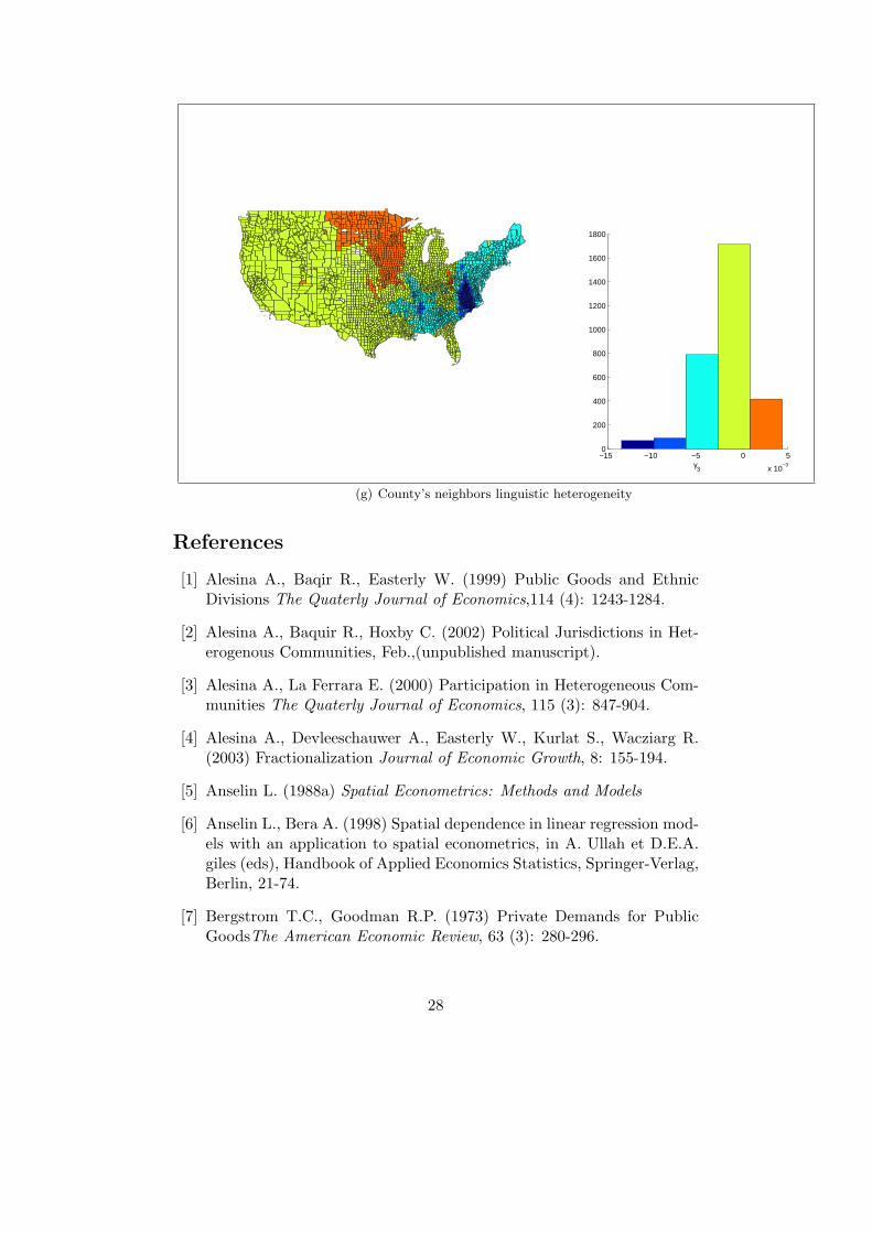
mated parameters for linguistic heterogeneity in the neighborhood of eachcounty (displayed in figure 3(f)) are only positive in the north part of thecenter of the country (namely, Minnesota, North and South Dakota, Iowa),while they are negative elsewhere. Finally, figure 3(g) demonstrates the pos-itive coefficients associated with income inequality in neighboring countiesare clustered partly in Texas, Pennsylvania and Wisconsin, while the nega-tive parameters are concentrated in the extreme North-East. The aspatialglobal estimation methods usually employed in the empirical studies maskthese spatial variations. This fact may lead to misleading conclusions.

6 Conclusion

In this paper the effects of population heterogeneity on the relative size ofthe nonprofit sector in the United States using county level data are investi-gated. Assuming that the relation under study is stationary over space, thespatial interdependence between U.S. counties are taken into account via aspatial (global) Durbin model. We show that in a global spatial setting, therelative size of the nonprofit sector in each county depends positively amongothers on the county’s linguistic heterogeneity and on the relative size ofthe nonprofit sector in the neighboring counties. According to our results,the relative size of the voluntary sector is more important in urban, moreeducated and richer counties. However, these results are only global in thesense that they ignore local spillovers that may occur. In a local setting,population heterogeneity and more particularly ethnic diversity and linguis-tic heterogeneity may affect the relative size of the nonprofit sector, but toa different extent and in a different manner according to the location.Future research may consist in developing a theoretical background to modelthe spillovers detected in this study. Besides, a Baysesian spatial local es-timation robust to heteroscedastic errors should be conducted in order tomake valid inferences on the estimates.

21

Appendix

Table 1: OLS, SEM

estimations OLS SEM tests OLS SEMconstant 0.0676

(0.0088)−0.0629(0.0152)

JB 3.372e+5

(0.000)-

frac 0.0643(0.0000)

0.0294(0.0017)

BP 2.629e+3

(0.000)2.639e+3

(0.273)

incineg −0.0177(0.0001)

−0.0117(0.0012)

KB 109.57(0.000) ()

otherlang −0.0010(0.0000)

−0.0004(0.0078)

Moran 26.32(0.000)

-

logpop 0.0069(0.0000)

0.0082(0.0000)

LMERR 679.03(0.000)

-

logurban 0.7702(0.0047)

0.9061(0.0014)

RLMERR 151.37(0.000)

-

poverty −0.0016(0.0031)

−0.0013(0.0000)

LMLAG 527.69(0.000)

-

education −0.0004(0.0436)

0.00067(0.0012)

RLMLAG 0.0308(0.8607)

-

age −0.0017(0.0000)

−0.00076(0.01155)

LM1 3308(0.000)

-

income 0.000004(0.0043)

0.000003(0.0000)

LM2 3308(0.000)

-

λ - 0.581(0.0000)

LMLAG* − 4.356e−10

(1)

R2 0.3107 0.4628 CF − −8.25026e+7

(0)

σ2 0.0026 0.002 - - -Notes: R2 is the adjusted measure of fit. JB is the Jarque-Bera normality test. BPdenotes the Breusch-Pagan heteroscedasticity test and KP a robust to non normal er-ror heteroscedasticity test. Moran is the Moran I-statistic. LMERROR and its robustversion named RLMERROR are Lagrange Multiplier (LM) tests for spatially autocor-related errors. LMLAG and its robust version RLMLAG are tests for omitted spatiallylagged dependent variable. LM1 is a joint test for spatial dependence and heterogeneity(Anselin, 1988, p71). It is the sum of BP and LMBI (and LMBI=RLMLAG+LMERRORor alternatively LMBI=LMLAG+RLMERR). LM2 is the joint test for heteroscedasticityand spatial autocorelation in the errors (Anselin, 1988, p121). It is the sum of BP andLMERR. CF is the Burridge (1981) common factor test.

22

Table 2: SDM (ML), BSDM(r=4),BMESS(r=200),BMESS(r=4)

estimations SDM BSDM BMESS(r=200) BMESS(r=4)constant 0.0964

(0.0007)0.0643(0.0004)

0.125(0.0000

0.0071(0.3695)

frac −0.005(0.6413)

0.0025(0.6993)

−0.005(0.334)

−0.00587(0.1975)

incineg −0.00796(0.028)

−0.00323(0.0977)

−0.0087(0.0125)

−0.0018(0.1885)

otherlang 0.0006(0.003)

0.00018(0.165)

0.0007(0.0000)

0.0001(0.1555)

logpop 0.0079(0.0000)

0.0062(0.0000)

0.0086(0.0000)

0.0072(0.0000)

logurban 0.83(0.0034)

0.522(0.0009)

0.9142(0.0005)

0.5888(0.0000)

poverty −0.0012(0.0005)

−0.00059(0.0029)

−0.0013(0.0005)

−0.0004(0.0375)

education 0.00174(0.0000)

0.0004(0.0076)

0.0017(0.0000)

0.0004(0.006)

age −0.00014(0.649)

−0.0010(0.0000)

0.00008(0.391)

−0.001(0.0000)

income 0.000003(0.0000)

0.000006(0.0000)

0.00003(0.0000)

0.000007(0.0000)

Wfrac 0.04167(0.0008)

0.0212(0.0074)

0.0395(0.002)

0.0073(0.21)

Wincineg −0.0074(0.307)

−0.0095(0.022)

0.00174(0.4365)

−0.005(0.2245)

Wotherlang −0.0012(0.0000)

−0.0008(0.0000)

−0.00127(0.0000)

−0.0004(0.011)

Wlogpop −0.00488(0.0061)

−0.0027(0.0175)

−0.0069(0.002)

−0.0054(0.0015)

Wlogurban −0.962(0.1117)

−0.5752(0.1155)

−1.1517(0.0975)

−0.8897(0.0925)

Wpoverty 0.0002(0.6766)

0.00047(0.11036)

−0.00009(0.439)

0.001(0.0045)

Weducation −0.0022(0.0000)

−0.0009(0.0000)

−0.0023(0.0000)

−0.0006(0.004)

Wage −0.0013(0.0072)

−0.0002(0.493)

−0.0019(0.0000)

0.0008(0.0315)

Wincome −0.000001(0.0000)

−0.000004(0.0000)

−0.000001(0.042)

−0.000005(0.0000)

alpha - - −0.8047(0.00000)

−1.472(0.0000)

rho - - 0.8878(0.00000)

0.9349(0.0000)

q - - 21.59(0.00000)

29.87(0.0000)

λ 0.528(0.0000)

0.46(0.0000)

0.5527(0.0000)

0.7705(0.0000)

R2 0.3570 0.2994 0.446 0.4σ2 0.0020 0.0027 0.0021 0.0005

23

Figure 3: Distribution of the means for 2000 vi estimates

1001 5000 10 000 15 000 20 000 25 000 30 000 35 000 40 000 45 000 50 000 560450

50

100

150

200

250

310

posterior mean of vi estimates

1001 5000 10 000 15 000 20 000 25 000 30 000 35 000 40 000 45 000 50 000 560450

50

100

150

200

250

310

posterior mean of vi estimates

county zip code from lowest to highest

Jefferson county (IA)

Jefferson county (MS)

Andrew county (MO)

Corson and Union counties (SD)

Chesapeake city (VA),Manassas Park city (VA)Norfolk city (VA),Richmond city (VA)Staunton city (VA),Suffolk city (VA)

Virginia Beach city (VA)

Randall county (TX)

Figure 4: Prediction error on center of area for various sum-sample size

0 500 1000 15000.016

0.017

0.018

0.019

0.02

0.021

0.022Smoothed LSDM Initial Holdout Residuals

Number of Local Observations

Abs

olut

e E

rror

24

Figure 5: Local spatial Durbin model parameter estimates based on m=456

0 0.2 0.4 0.6 0.80

200

400

600

800

1000

1200

1400

λ

(a) County’s Spatial dependence

−0.15 −0.1 −0.05 0 0.05 0.10

500

1000

1500

β2

(b) County’s ethnic heterogeneity

25

−0.04 −0.03 −0.02 −0.01 0 0.010

100

200

300

400

500

600

700

800

900

β3

(c) County’s income inequality

−2 −1 0 1 2 3 4 5

x 10−3

0

200

400

600

800

1000

1200

1400

1600

1800

β4

(d) County’s linguistic heterogeneity

26

−0.2 −0.1 0 0.1 0.2 0.30

500

1000

1500

2000

2500

γ1

(e) County’s neighbors ethnic heterogeneity

−0.1 −0.05 0 0.05 0.10

200

400

600

800

1000

1200

γ2

(f) County’s neighbors income inequality

27

−15 −10 −5 0 5

x 10−3

0

200

400

600

800

1000

1200

1400

1600

1800

γ3

(g) County’s neighbors linguistic heterogeneity

References

[1] Alesina A., Baqir R., Easterly W. (1999) Public Goods and EthnicDivisions The Quaterly Journal of Economics,114 (4): 1243-1284.

[2] Alesina A., Baquir R., Hoxby C. (2002) Political Jurisdictions in Het-erogenous Communities, Feb.,(unpublished manuscript).

[3] Alesina A., La Ferrara E. (2000) Participation in Heterogeneous Com-munities The Quaterly Journal of Economics, 115 (3): 847-904.

[4] Alesina A., Devleeschauwer A., Easterly W., Kurlat S., Wacziarg R.(2003) Fractionalization Journal of Economic Growth, 8: 155-194.

[5] Anselin L. (1988a) Spatial Econometrics: Methods and Models

[6] Anselin L., Bera A. (1998) Spatial dependence in linear regression mod-els with an application to spatial econometrics, in A. Ullah et D.E.A.giles (eds), Handbook of Applied Economics Statistics, Springer-Verlag,Berlin, 21-74.

[7] Bergstrom T.C., Goodman R.P. (1973) Private Demands for PublicGoodsThe American Economic Review, 63 (3): 280-296.

28

[8] Brock W and Durlauf S. Growth Empirics and Reality, World BankEconomic Review, 15, 3: 229–272, 2001.

[9] DiMaggio P.J., Anheier H.K. (1990) The Sociology of Nonprofit Orga-nizations and Sectors Annual Review of Sociology, 16 :137-159.

[10] Durlauf S. N. (2002) On The Empirics of Social Capital, The EconomicJournal, 112: 459–479.

[11] Durlauf S.N., Fafchamps M. (2003) Empirical Studies of SocialCapital: A Critical Survey, www.ssc.wisc.edu/econ/archive/wp2003-12.pdf.2003.

[12] Ertur C., Le Gallo J., LeSage J.P. (2003) Local versus Global Conver-gence in Europe: A Bayesian Spatial Econometric Approach. REALDiscussion paper, REAL 03-T-28.

[13] Ertur C., Koch W. (2005) Growth, Technological Interdependence andSpatial Externalities: Theory and Evidence.

[14] James E. (1993) Why Do Different Countries Choose a DifferentPublic-Private Mix of Educational Services? The Journal of HumanRessources, 28 (3): 571-592.

[15] Lassen D.D. (2006) Ethnic Divisions, Trust, and the Size of the In-formal Sector Journal of Economic Behaviour & Organization Vol.xxx(2006)xxx-xxx (article in press).

[16] Lesage J.P (1997) Bayesian Estimation of Spatial Autoregressive Mod-els International Regional Science Review, 20: 113-129.

[17] McMillen D.P. (1996) One Hundred Fifty Years of Land Values inChicago: A Nonparametric Approach. Journal of Urban Economics 40:100-124.

[18] Miguel E., Gugerty M.K. (2004) Ethnic Diversity, Social Sanctions, andPublic Goods in Kenya. Unpublished manuscript available at http ://emlab.berkeley.edu/users/emiguel/miguel tribes.pdf

[19] Okten C., Osili U.O. (2005) Ethinic Diversity and Charitable Giv-ing. Unpublished manuscript available at http : //team.univ −paris1.fr/espe2005/papers/osili paper.pdf

[20] Pace R.Kelley, LeSage J.P (2000a) Closed Form Maximum LikelihoodEstimates for Spatial Problems. Unpublished manuscript available athttp : //www.spatial − statistics.com

[21] Pace R.Kelley, LeSage J.P (2000b) Using Matrix Exponentials to Ex-plore Spatial Structure in Regression relationship.

29

[22] Pace R.K., Barry R. (1997) Quick Computation of Regression s witha Spatially Autoregressive Dependent Variable. Geographical Analysis,39(3):232-247.

[23] Pace R.K, LeSage J.P (2004) Spatial autoregressive local estimation.Recent Advances in Spatial Econometrics Getis Arthur, Mur Jesus andHenri Zoller (eds), Palgrave Publishers, 3:31-51.

[24] Rose-Ackerman S. (1996) Altruism, Nonprofits, and Economic TheoryJournal of Economic Leterature, XXXIV: 701-728.

[25] Salamon L.M., Sokolowski S.W., Anheier H.K. (2000) Social Originsof Civil Society: an Overview Working Papers of The Johns HopkinsComparative Nonprofit Sector Project, Johns Hopkins University.

[26] Weisbrod B. (1977) The voluntary nonprofit sector: an economic anal-isys. Lexington Books D.C. Health & Co Lexington, MassachusettsToronto.

[27] Weisbrod B. (1986) Toward a Theory of the Voluntary Nonprofit Sectorin a Three-sector Economy in The Economics of Nonprofit Institutions,ed. S.Rose-Ackerman, Columbia University.

30