NBER WORKING PAPER SERIES

POPULISTS AT THE POLLS:ECONOMIC FACTORS IN THE 1896 PRESIDENTIAL ELECTION

Barry EichengreenMichael R. Haines

Matthew S. JaremskiDavid Leblang

Working Paper 23932http://www.nber.org/papers/w23932

NATIONAL BUREAU OF ECONOMIC RESEARCH1050 Massachusetts Avenue

Cambridge, MA 02138October 2017

For helpful comments we thank Price Fishback, Jonathan Kirshner, Frances Lee, Eric Schnickler, Richard Sutch and Gavin Wright. We also thank Alison Rice-Swiss for editorial assistance. The views expressed herein are those of the authors and do not necessarily reflect the views of the National Bureau of Economic Research.

NBER working papers are circulated for discussion and comment purposes. They have not been peer-reviewed or been subject to the review by the NBER Board of Directors that accompanies official NBER publications.

© 2017 by Barry Eichengreen, Michael R. Haines, Matthew S. Jaremski, and David Leblang. All rights reserved. Short sections of text, not to exceed two paragraphs, may be quoted without explicit permission provided that full credit, including © notice, is given to the source.

Populists at the Polls: Economic Factors in the 1896 Presidential ElectionBarry Eichengreen, Michael R. Haines, Matthew S. Jaremski, and David LeblangNBER Working Paper No. 23932October 2017JEL No. N0,N11

ABSTRACT

The 1896 presidential election between William Jennings Bryan and William McKinley has gained new salience in the wake of the 2016 contest. We provide the first systematic analysis of voting patterns in 1896, combining county-level returns with economic, financial, demographic and climatological data. Specifically, we consider the economic concerns of the Populists with falling crop prices, high interest rates and railroad monopolies. We show that Bryan did well where mortgage interest rates were high, railroad penetration was low, and crop prices had declined by most over the previous decade. Using our estimates, we show that further declines in crop prices or increases in interest rates would have been enough to tip the Electoral College in Bryan’s favor. But to change the outcome, the additional fall in crop prices would have had to be large. The counterfactual increase in interest rates appears, at first blush, to have been more modest. But where previous authors have argued that interest rates came down in the 1890s because of the entry of additional banks, our estimates indicate that bank entry would have had to be very significantly slower to tip the election. There is no question that economic grievances mattered in 1896. But small or even moderate changes in economic conditions would not have changed the outcome of the election.

Barry EichengreenDepartment of EconomicsUniversity of California, Berkeley549 Evans Hall 3880Berkeley, CA 94720-3880and NBEReichengr@econ.Berkeley.edu

Michael R. HainesDepartment of Economics, 217 Persson HallColgate University13 Oak DriveHamilton, NY 13346and NBERMHAINES@MAIL.COLGATE.EDU

Matthew S. JaremskiColgate UniversityDepartment of Economics13 Oak DriveHamilton, NY 13346and NBERmjaremski@colgate.edu

David LeblangDepartment of Political ScienceUniversity of VirginiaS281 Gibson HallCharlottesville, VA 22904leblang@virginia.edu

1

Populists at the Polls:

Economic Factors in the 1896 Presidential Election

Barry Eichengreen, Michael Haines, Matthew Jaremski and David Leblang 1

September 2017

“You come to us and tell us that the great cities are in favor of the gold standard; we reply that the great cities rest upon our broad and fertile prairies. Burn down your cities and leave our farms, and your cities will spring up again as if by magic; but destroy our farms and the grass will grow in the streets of every city in the country. My friends, we declare that this nation is able to legislate for its own people on every question, without waiting for the aid or consent of any other nation on earth.”

William Jennings Bryan Speech at the Democratic National Convention July 9, 1896

1. Introduction

The 1896 Presidential Election broke the mold of American politics. To face off against a Republican establishment candidate, William McKinley, the Democrats nominated a political outsider, William Jennings Bryan. In doing so they sought to capitalize on the anger of farmers and workers, who blamed their troubles on wealthy businessmen, railroad monopolists, Eastern bankers and distant politicians. Bryan’s fiery speeches, impassioned advocacy of bimetallism and fierce defense of the common people, in addition to appealing to Democrats, appealed to Populists, supporters of the third party of agrarian origin that arose out of dissatisfaction with the two establishment parties.

The 1896 campaign, capped by Bryan’s narrow loss, has long been seen as a turning point. Authors like Sundquist (1983) characterize it as the first 20th century presidential campaign. McKinley raised unprecedented amounts of campaign funds and mounted a nation-wide campaign organization. In contrast, Bryan’s unconventional campaign eschewed the media, which was arrayed against him, in favor of a new approach designed to facilitate direct communication with voters, which notably featured the first nationwide whistle-stop campaign.

The outcome, authors like Schattschneider (1960) and Burnham (1965) argued, represented a “fundamental realignment” of American politics. It inaugurated what they characterized as the “Fourth Party System,” distinguished by Republican dominance of the White House and Congress; between 1896 and 1932 the Democrats elected only one president, Woodrow Wilson, in 1912 when the Republican Party split.2 This era was characterized by declining voter turnout and weakened public participation, reflecting the extent to which the political and economic establishment was now effectively insulated from “mass pressures.”3 1 University of California, Berkeley; Colgate University; Colgate University; and University of Virginia, respectively. For helpful comments we thank Price Fishback, Jonathan Kirshner, Frances Lee, Eric Schnickler, Richard Sutch and Gavin Wright. We also thank Alison Rice-Swiss for editorial assistance. 2 As Sundquist (1983) describes, states that had been evenly split between the parties (California, Connecticut, Indiana, New Jersey and New York) and even traditional Democratic strongholds like Delaware and West Virginia became solidly Republican. 3 These authors build on the influential work of Key (1955), who referred not to fundamental realignments but critical elections, and who similarly highlighted the importance of 1896.

2

Nothing less than the massive political and economic shock of the Great Depression was required to overturn this established state of affairs. As Schattschneider (1956, p. 201) put it, the 1896 election “determined the nature of American politics from 1896 to 1932.”

Subsequent authors like Mayhew (2002) have challenged many of these specific assertions. But their revisionism does not diminish the prominence of the 1896 election in the literature of political science. Political scientists continue to debate the causes of McKinley’s victory, weighing the influence of improving agrarian conditions following the depressed crop prices and severe droughts of the late 1880s and early 1890s against secular trends in the economy and society such as urbanization, industrialization and immigration (see e.g. Jensen 1971).

For economic historians, the significance of the 1896 election lies in its role in essentially settling the debate over free silver and tariff protection for a generation. Prior to 1896, both policies had been contested for the better part of two decades. Starting in1896, the status quo established following McKinley’s victory stayed in place for four decades.4

In addition, the 1896 election has always held special fascination for economic historians because of the prominence of economic issues and events in the campaign and, arguably, the outcome. These issues and events range from the 1893 financial crisis and recession to the regulation of economic activity and immigration and the aforementioned controversies over free silver and tariffs. Those emphasizing economic issues point to the complaints of farmers about mortgage interest rates and railroad freight rates. They point to depressed crop prices as a source of distress affecting rural voters. They cite the particular concerns of tobacco farmers about the monopsonistic marketing practices of the American Tobacco Company and of cotton farmers over what they saw as the exploitative nexus of sharecropping, debt peonage and pressure to engage in monoculture. Equally, they point to the dissatisfaction of industrial workers with long hours, dangerous conditions and insecurity of employment, and with the monopsony power of large employers that resulted in those conditions (see e.g. Durden 1965). Many of these issues were prominently associated with the Populist Party, but they were also coopted by the Democrats, especially in the South, on whose ticket Bryan also ran. As Kousser (1974, p.38) puts it, “By the mid-nineties, no (Democratic) stump speech in the South was complete without blasts at the railroads, the trusts, Wall Street, the gold bugs, the saloonkeepers or some similarly evil ‘Interest’.”

Not all analysts of the election agree, however, about the dominance of economic issues relative to social and identity concerns revolving around race, ethnicity and religion. When selecting a presidential candidate to support, voters split along racial and religious lines and over social issues like prohibition and immigration. Protestants, it is said, voted disproportionately for Bryan, Catholics for McKinley. Blacks, where they could vote, voted for the party of Lincoln. Seen from this perspective, the 1896 election had a prominent identity cast.

4 In other words, the status quo remained until the gold standard was suspended 37 years later, in 1933, and the Reciprocal Trade Agreements Act allowing the president to negotiate tariff reductions was passed 38 years later, in 1934. Some of the early “realignment literature” argued that the 1896 election brought about important changes in policy (“policy innovations”). Our characterization here is that it was important instead for establishing continuity (cementing the gold-standard and protective-tariff status quo), consistent with the later conclusion of Burnham (1986).

3

At the same time, the 1896 contest is sometimes seen as a so-called deviant election in which the parties departed from their traditional identity politics. Democrats had long been seen as friendlier to Catholics and immigrants, Republicans as more hospitable to Protestant evangelicals and native-born stock. But Bryan’s campaign was anomalous relative to elections both prior and subsequent to 1896, in that he appealed to identity groups that were traditionally affiliated with the Republican Party. Therefore, his candidacy could conceivably have reduced rather than accentuated the usual effect of social identity in U.S. presidential elections. Scholars consequently question whether these social and identity issues, as opposed to economic dissatisfaction and self-interest, in fact carried the electoral day.

One reason these questions remain unanswered is that the empirical literature on the period focuses on the validity of the Populists’ arguments, measuring the agricultural terms of trade, interest rates, the growth of manufacturing employment and wages for example, without also seeking to understand their electoral implications, much less to weigh the electoral implications of those economic grievances against those of social concerns and identity politics. To put it another way, the literature has focused on why the Populists’ were angry and whether their anger was justified, not on whether that anger informed their voting decisions. Bowman (1965), North (1966), and Shannon (1968) all provide evidence, for example, that the agricultural terms of trade in were improving. Bowman and Keehn (1974) find that there were at most a few periods of brief cyclical deterioration in the agricultural terms of trade superimposed on an improving trend. Concluding that farmers were not suffering, they imply but do not show that low farm-gate prices could not have been the source of the Populists’ gains in the polls in the 1890s. Similarly, while McGuire (1981) and Halcoussis (1996) document the extent of instability and unpredictability in agriculture in this period and suggest that this was an important source of agrarian unrest, they do not explicitly connect these patterns to political behavior. And while Aldrich (1980) points to sharp cyclical increases in railroad freight rates in the late 1880s and early 1890s as motivation for Populist sentiment, he does not draw a quantitative link to voting patterns.

Thus, the literature has thrown up a rich menu of hypotheses about how economic and other factors may have influenced the 1896 election, but the link with actual voting remains unclear. These studies provide various degrees of support for the Populists’ complaints, but they do not take the next step of mapping their economic condition into electoral outcomes, much less weighing their role relative to those of social issues and identity politics.

Bryan lost by just 50 electoral votes, and the outcome was strikingly close in many states, counties and districts. According to Williams (1936, p. 193), Bryan was a mere 19,436 votes from winning the states needed to secure the Electoral College and the presidency.5 Given this, one can imagine that relatively small changes in economic conditions could have reversed the outcome of the election and altered the course of American history. As noted above, the election and subsequent Republican dominance resulted in substantial import tariffs, adherence to the gold standard and relatively limited regulatory intervention by the federal government up to and into the 1930s. Only during the Great Depression did the U.S. shift to managed money (with

5 One is reminded of calculations by observers of the 2016 election that Hilary Clinton would have won the Electoral College with just 77,000 additional votes concentrated in three states (Pennsylvania, Wisconsin and Michigan) http://www.weeklystandard.com/the-election-came-down-to-77744-votes-in-pennsylvania-wisconsin-and-michigan-updated/article/2005323.

4

abandonment of the gold standard), freer trade (with adoption of the Reciprocal Trade Agreements Act) and more stringent market regulation (with the Glass-Steagall Acts, the Securities Exchange Act, and other New Deal-era regulatory initiatives). With a small swing in votes in 1896, the implication follows, this shift to different policies might have occurred much earlier.6

The role of these factors in the 1896 campaign is of even greater interest in the wake of the 2016 U.S. presidential election. In many ways, Donald Trump’s campaign paralleled Bryan’s. Both candidates ran as political outsiders. Both largely repudiated their party’s leadership and fundraising apparatus. Both spoke directly to voters in large rallies. Both ran against a political establishment dominated by elites who, they said, were incapable of representing the interests of the people (Frum 2016). And there is a dispute over the role of economic versus social factors, or identity politics, in the outcomes of both the Bryan-McKinley and Trump-Clinton elections (see Inglehart and Norris 2016).

But if the 1896 and 2016 elections were similar in these and other respects, there was one momentous difference: while Trump won, Bryan lost. One possible explanation for the contrast is the evolution of economic variables. Where Trump benefited from the dissatisfaction with the political establishment stemming from the slow recovery of the economy from the Great Recession of 2007-2009, Bryan was hurt by strong recovery from the Panic of 1893.7 In addition, crop prices began rising in 1896, which further favored economic policy continuity and the mainstream candidate, McKinley. No less an expert than Karl Rove (2015) argues that McKinley owed his victory to improving economic conditions.

Or perhaps Bryan was less effective at tapping into identity politics. In contrast to Trump’s pointed anti-immigrant and anti-foreigner rhetoric, Bryan did not launch an aggressive anti-new-immigrant campaign in an effort to galvanize old-immigrant voters. Instead he singled out certain small immigrant groups like the Chinese and Japanese. As a political outsider, he found it difficult to win the support of Eastern Catholics and immigrants, who were traditionally aligned with the Democratic Party, as well as other groups, like Southern blacks, with reason to feel that they had been disfavored by the political establishment and that might conceivably have been attracted by a Populist candidate. He was unsuccessful at broadening his appeal from disaffected farmers to urban workers worried about their prospects in an American economy increasingly dominated by large corporations (Faulkner 1969).

Given all this, it is striking that there exists no systematic empirical analysis of voting patterns in 1896.8 Providing one is our goal in this paper. We combine county-level voting results with economic, financial, demographic and climatological data from the 1890s. We

6 The implications for policy would have also depended, of course, on the outcome of Congressional elections, since a president makes policy, economic policy in particular, in conjunction with the Congress. Since Senators at the time were appointed by their state legislature rather than through direct election, a full Congressional counterfactual is even harder to undertake than today (and is therefore beyond the scope of this paper). 7 The estimates of Balke and Gordon (1989) put real GNP in 1896 fully 16 per cent above the post-crisis trough in 1894. Where Obama experienced a u-shaped recovery, McKinley enjoyed a v-shaped recovery. 8 The closest approximation we have been able to find is Klepper (1978) who uses state-level data to estimate the impact of the agricultural share of employment, the racial composition of state populations, and related variables to the share of the vote garnered by agrarian “protest parties” in elections prior to the 1896 fusion between the Populists and Democrats. Since only 24-some states had such parties on the ballot, the resulting cross sections are very small.

5

consider the economic concerns of the Populists over falling crop prices, high interest rates and railroad monopolies, as well as social, demographic and identity factors like race, religion, national origin, geography, and urban versus rural residence. We use the results to ask whether small changes in economic circumstances, say modestly higher interest rates, limited declines in crop prices, or further reductions in railway penetration and competition, could have tipped the outcome in Bryan’s favor.

We confirm that Bryan did poorly in counties with large shares of Catholics, reflecting the candidate’s Protestant-Liberal bent. He did poorly in counties with large shares of foreign-born residents. He did poorly in counties with large black populations, reflecting their allegiance to the Party of Lincoln and the fact that Bryan was allied with Southern Democrats who were actively seeking to disenfranchise black citizens.9 He did poorly in areas with high levels of manufacturing activity.

But even when controlling for these racial, ethnic, religious and sectional variables, we still find a significant role for the Populists’ economic concerns. Bryan’s vote share was higher in counties where interest rates were high and in counties with low railroad mileage per square mile, which we interpret in terms of railway penetration and competition. Bryan also did well in counties where farmers experienced relatively large declines in crop prices prior to the election. He did especially well, over and above what would have been predicted by the decline in crop prices, in counties where farmers were disproportionately engaged in cotton and tobacco production, reflecting the special concerns of cotton and tobacco farmers.

Economic conditions appear, then, to have had a significant impact on voting; the question is whether that effect was large enough to tip the election. Using our estimates to create a counterfactual Electoral College, we show that further declines in crop prices or increases in interest rates would have been enough to tip the election in Bryan’s favor, but not so lower levels of railway penetration or more extreme climatic conditions. There is in fact no level of railway penetration sufficient to have tipped the Electoral College balance in Bryan’s favor, for example. In contrast, there is such a level for the change in crop prices and for interest rates.

But the counterfactual decline in crop prices would have had to be very large. The average fall would have had to be nearly twice that which actually occurred between 1886 and 1895. Only 1 ½ per cent of U.S. counties in fact experienced a crop-price decline of this magnitude in the 1886-95 period.

The counterfactual increase in interest rates needed to tip the Electoral College balance appears, at first blush, to have been more modest, on the order of 2 percentage points, from the prevailing average of 8 per cent. Interest rates of 10 per cent were far from unheard of. Some 14 per cent of U.S. counties had mortgage interest rates this high or higher in 1890.

Previous authors have argued that interest rates came down in the 1890s, or more precisely that they were lower than they would have been otherwise, because of the entry of additional banks. This entry, reflecting the reduction of capital requirements for state banks and the passage of general banking laws, led to growing competition among lenders and downward 9 Some of whom had joined “paramilitary outfits or whitecap raids” directed in part against “poor black folk” (Hahn 2003, p.432). Hahn (2003) also describes instances when black Republicans who maintained the ability to vote allied with Southern Populists in local and congressional elections, but these, broadly speaking, were the exceptions to the rule.

6

pressure on interest rates, with evident electoral implications. While we confirm the existence of a significant negative relationship between the number of banks and interest rates at the county level, our estimates indicate that a very substantial decline in bank entry and, indeed, rise in exit would have been required to achieve interest rates at the required level (i.e., 2 additional percentage points relative to prevailing levels in 1890). According to our sources, the number of state and national banks rose from 6,751 in 1890 to 9,096 in 1896, or by about 1 bank per county. Estimates using county-level data relating the level of interest rates to the number of banks suggest that the number of banks would have had to fall by 28 banks per county, on average, to bring rates down by the 2 percentage points needed to tip the Electoral College to Bryan. This would have represented an enormous swing from the rate of entry actually observed in the first half of the 1890s. Even with a counter-factual where no county has a commercial bank, the estimates still do not suggest interest rates would have averaged over 10 percent.

Our results thus suggest that while economic variables mattered significantly in the 1896 election, there would have had to have been very substantial changes in any one of those variables, relative to observed trends, to swing the Electoral College to Bryan. To be sure, one can also imagine combinations of counterfactual changes in economic variables altering the outcome of the election. But changes in the key variables would still have had to be substantial. Notwithstanding the salience of economic grievances in 1896, small or moderate changes in economic conditions –lower crop prices or slower bank entry rates – would not have been enough to alter the outcome of the election.

2. Historical Narrative

Bryan’s nomination and the platform on which he ran must be understood in terms of the agrarian unrest that developed in the course of preceding decades. Farmers, sometimes allied with miners and manufacturing workers, banded together in an effort to advance legislation that would ease their burdens and right the perceived wrongs of which they complained. To this end, they formed the succession of proto-populist and populist movements that are our focus here. While we refer to these groups generically as Populists, there was actually a series of politically influential agricultural interest groups between 1870 and 1900. These included the Grange in the early to mid-1870s, the Farmers Alliance in the 1880s, and finally the Populist (or Peoples) Party in the 1890s (see Hicks 1931 and Nordin and Walker 1974).

While there were differences in the composition and platforms of these groups, their arguments bore a family resemblance. Their common complaint was that economic growth and change since the Civil War had made it increasingly difficult for them to succeed, where by economic growth and change they meant in particular farm-gate prices, freight rates and the cost of credit. They complained further of the absence of an adequate political response to their problems and that, to the contrary, they were increasingly dispossessed politically. As North (1966, p.145) put it: “this was the era when [the farmer] was becoming a minority in America. Throughout all of our earlier history, his had been the dominant voice in politics and in an essentially rural society. Now, he was being disposed by the growing industrial might of America and its rapid urbanization.”

The problems perceived by the Populists were tied to the expansion of agriculture westward, the growing importance of manufacturing, and the commercialization of the economy. The Homestead and Pacific Railroad Acts of 1862 opened the West to settlers. While this westward push made it cheaper to purchase land, topsoil was not as deep as further east, and

7

climate was more variable. In areas characterized by these conditions, farmers needed more land and labor-augmenting equipment in order to turn a profit, which in turn heightened their dependence on credit. Moreover, farming in newly settled areas subject to extremes of temperature and precipitation often dictated specializing in a single cash crop. Specialization increased the volatility of yields and heightened the risk of crop failure to the extent that the stabilizing benefits of diversification were foregone. It also limited self-sufficiency and exposed the farmer to anonymous market forces. The shift to commercial agriculture, the need for credit, and exposure to crop-price and transportation-cost shocks seemed to grow larger with each passing year, according contemporaries (Mayhew 1974).

Farmers complained specifically of adverse price movements. Although the overall price-level in the economy was declining in the decades prior to 1896, farmers insisted that the prices of agricultural goods were declining at even faster than the prices of manufactured goods produced in the East. To the extent that this was true, the decline in the agricultural terms of trade made it harder for farmers to maintain their standard of living, in contrast to Eastern manufacturers, who benefited from cheaper agricultural inputs. As noted above, subsequent studies dispute these assertions, showing that the price of agricultural commodities relative to manufactured goods was broadly flat and sometimes even rising. But this was not the impression of contemporaries, if their political rhetoric is to be believed.

Tobacco and cotton farmers voiced additional complaints about marketing conditions, above and beyond the contemporaneous fall in prices. The decline in cotton and tobacco prices was actually relatively mild compared to the overall decline in farm prices.10 But tobacco growers feared the implications for future prices of the creation in 1890 of the American Tobacco Company (“the tobacco trust”) with its singular leverage and monopsony of loose-leaf tobacco. The five big cigarette producers were merged into one company in 1889 under the leadership of James B. Duke. Previously, Tennessee and Kentucky tobacco farmers could sell their crop to a local merchant or sell it directly to manufacturers at a regional warehouse or from his own barn.11 Now “[c]ompeting buyers for tobacco disappeared as the agents for the American Tobacco Company dictated the prices farmers received” (Campbell 1993, p.2). Creation of the American Tobacco Company fanned fears not simply of monopsony power today but of the possibility that farm-gate prices would be driven down still further tomorrow.12

In the case of cotton, the agent with market power was not a nation-wide trust but rather the local furnishing merchant, who was a “territorial monopolist” in the language of Ransom and Sutch (1977, p.127). Cotton growers, both white and black and tenant and sharecropper alike, complained that these local merchants were the only available buyers of their product or that they effectively exercised exclusive right to purchase that product as a result of earlier extension of credit through the crop-lien system. Specialized cotton factors, who prior to the Civil War had purchased the output of large plantations and provided their owners with credit, now found it

10 Six per cent for both tobacco and cotton versus 22 per cent for the average agricultural portfolio over the period 1886-1895; see also Section 6 below. 11 Campbell (1993), p.26. 12 In addition, tobacco farmers had reason to worry about the spread of Granville Wilt, a bacterial disease first observed in Granville County, North Carolina, in 1881, but which spread to additional farms further afield in the first part of the 1890s (Olmstead and Rhode 2008). The problem was tracked by the U.S. Department of Agriculture, which was unable to do anything about it, however, until the bacteria was identified and classified after the turn of the century.

8

uneconomical to deal with large numbers of small, dispersed farmers, and the local merchant occupied this niche in their absence. Sometimes lien agreements specified the price offered by the merchant in advance of the harvest, while in others they stated that the cotton in question would be bought “at the customary price,” whatever that meant (Woodman 1968, p.299-300). Either way, it is not hard to imagine, in the absence of competition in the provision of supplies on credit, that the merchant had scope for manipulating that price.

Farmers further complained that these local merchants refused to provide credit on any crop other than cotton, thereby applying pressure for their customers to expand cotton acreage in order to make good on their credit obligations. This increased the farmers’ dependence on monoculture, with all its associated risks. It had the further consequence of effectively driving cotton prices down still further. In some rural areas, banks were absent; in others where they were present, they refused to take crop liens. Either way, the farmer was left with little choice but to rely on the furnishing merchant (Wright 1986, p.112; Hahn 2003, p.432). In the 1880s, the Southern Farmers’ Alliance provided temporary relief by creating cooperatives to supply members with credit, at a reasonable price, to purchase supplies and to market the crop, but most of these cooperatives had failed by the early 1890s.13

Cotton farmers were also hit by a sharp increase in the cost of the burlap material used to wrap cotton bales. In 1888, a cartel of burlap manufacturers succeeded in raising the price of jute wrapping by more than 60 per cent. Suppliers raised the price just before the harvest, leaving farmers no time to seek out alternatives. The financial impact of this jump in the price of jute on cotton growers was “significant” (McMath 1993, p.95). By the time of the 1889 harvest, the Southern Farmers’ Alliance was able to organize supplies of cotton wrapping and persuade farmers to use it. Unfortunately, only a few Southern cotton mills had the equipment needed to manufacture the cloth needed, and the major cotton exchanges still expected wrapping to be in jute. Some historians regard the Alliance jute boycott as a success, but others observe that the jute cartel outlived the Alliance, and that jute producers were able to drive the price back up in the 1890s (McMath 1993, p.97).14

As more farmers moved into commercial cultivation, they found themselves depending on the railroads to move their crops. With limited ability to store across years or sell locally, they had to pay what the railroads asked. Dakota farmers complained that freight absorbed as much as half of the price of their corn and oats and a third of the price of their wheat (Farmer 1924, p.424). While real rail transportation costs declined between 1870 and 1880, Aldrich (1980) found that they rose steeply thereafter, peaking in the late 1890s. This was in contrast to other transportation costs, which remained steady after 1880.

Farmers complained further that they were charged higher rates than railway customers who lived in cities or shipped long distances. The railroads had a ready rationalization for the 13 Whether this was due to low cotton prices, the success of state and private banks in withholding credit from the cooperatives is disputed (Woest 1998, p.23). McMath (1993) argues further that the cooperatives of the Southern Alliance created what was effectively a social and political network that encouraged additional farmers to ally with the Populist camp. 14 In addition, cotton growers had their equivalent of Granville Wilt, in the form of Fusarium Wilt, which had infected large sections of South Carolina, Georgia and Alabama by the end of the 19th century (Olmstead and Rhode 2008, p.135). The boll weevil, while ultimately developing into a larger problem, did not begin spreading until 1892-3. The U.S. Department of Agriculture sent investigators into the field in 1894-5, but their initial ideas about how to contain it spread proved ineffectual, which could not have reassured disaffected cotton growers.

9

practice. As Hicks describes (1931, p. 61): “The railroads figured, not without reason, that large shipments cost them less per bushel to haul than small shipments. Accordingly, on through routes and long haul where there was a large and dependable flow of freight the rates were comparatively low…Sometimes the western local rate would be four times as great as that charged for the same distance and the same commodity in the East.” Whatever the rationale for the practice, it did not make the farmers happy.

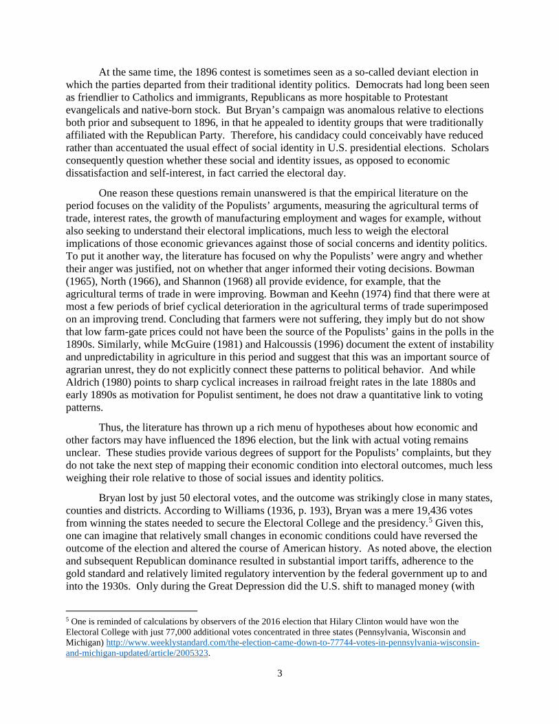
Rates were also perceived to vary with the intensity of competition between lines. Many sparsely settled Western states saw limited railway construction and were served by a single railroad or only small handful of companies. Magliari (1989, p. 450) argues that Populism in California, for example, was “primarily aimed at the Southern Pacific Railroad’s monopoly of the shipment of grain to tidewater.” The map of railroad miles per square mile in Figure 1 is broadly consistent with this view. Railroad density is low in the West, including in California, with few exceptions (the areas extending north and east from San Francisco, east from Portland, west from Spokane and Walla Walla, and in the environs of Denver and Salt Lake City, the latter being areas where feeder lines and transcontinental railways met). It is highest in the Midwest and Northeast. Much but not all of the South, like the West, was underserved by railroads according to this measure.

While prices were likely to be high in monopolistic markets with only a single rail, prices were not always significantly lower in areas with multiple railroads. Hicks (1931) in his classic account of the Populist Revolt argued that even when several railroads coexisted in an area they developed anti-competition agreements designed to keep rates high. Subsequent studies like Porter’s (1983) analysis of the Joint Executive Committee, which oversaw the railway cartel extending from Chicago to the Eastern Seaboard, temper this conclusion by identifying periods of cartel breakdown in the early and mid-1880s. But Porter’s analysis extends only through 1886, since he argues that the adoption of the Interstate Commerce Act of 1887, and specifically Section 5 of the Act which outlawed the pooling of freight or revenue by independent railways, dealt a blow to the collusive practices. MacAvoy (1965), in an earlier, less formal study, distinguishes a period of continued strong cartelization before 1894, then a period of evasion and “rate demoralizations” in 1894-5, and finally renewed strengthening of the railroad cartel in 1896 itself. Ulen (1980) questions whether the Interstate Commerce Commission was effective at any point in its first ten years of operation.15

Finally, there is the fact that many farmers relied on funding from banks and other financial intermediaries to purchase land and equipment, to buy seed during planting season, and to obtain other necessities before harvest. Interest rates were particularly high in the agricultural regions, where risk was exceptional, and in rural areas without sufficient population to support a bank, much less a number of competing institutions (Eichengreen 1984). They varied depending on whether credit was obtained from a bank or insurance company subject to usury laws, or from merchants, suppliers or other nonbank sources less constrained by that legislation. Where interest rates were high, farmers could not always obtain the land, supplies and equipment they required. And even where they could borrow at the prevailing high rates of interest, leverage implied bankruptcy in the event of adverse movements in crop prices.

15 Be this as it may, we would emphasize the importance of distinguishing two issues: whether or not separate railroads effectively colluded, and whether or not this was the perception of farmers and other voters.

10

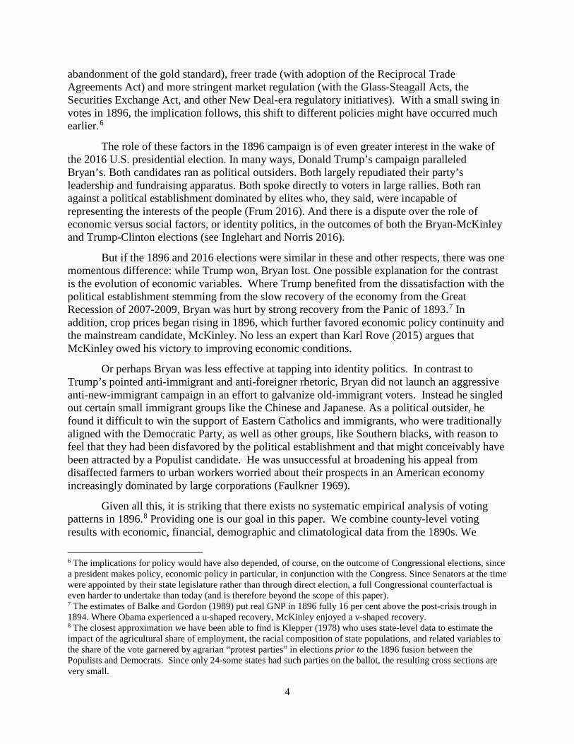
Such complaints grew louder in the late 1880s and early 1890s when many banks turned away mortgage lending. Farmer (1924, p.419) writes that with the onset of drought in the late 1880s, farmers who had previously borrowed via real estate mortgages were “forced to resort to chattel loans, securing such money as he could upon his livestock and farm machinery. These loans bore higher interest rates than the farm mortgages – many of them from twenty to thirty-six per cent.” Farmer was particularly concerned with interest rates in underbanked parts of the Central Plains, West and South.16 While regional interest rate gaps declined during the period, as famously established by Davis (1965), rates were still substantially higher in the mid-1890s in the South and Great Plains than in New England and the Middle Atlantic (see Figure 2).17

These complaints gained salience with financial dislocations and distress following the panics of 1884, 1890, and 1893. Interruptions to credit supplies and shocks to interest rates were always disruptive, but the problem was more severe now that agriculture was commercialized, specialization was higher, and leverage was greater. These panics, rather than being driven by local conditions, were widely seen as resulting from speculation and illiquidity in distant money centers. Banks prohibited from branching placed money on deposit in larger cities, in order to clear checks and satisfy reserve requirements. This meant that money flowed from rural areas to large cities (particularly New York City) where it was invested in the call loan market. A shock to New York City could therefore immobilize the entire nation’s reserves and transmit the panic outward, notably to credit-dependent farming regions. (Sprague 1910; Calomiris and Gorton 1991; Wicker 2000)

The Populists' response took two forms. First, they argued for expanding the money supply. The Crime of ’73, when Congress essentially demonetized silver, was a rallying point for farmers and miners. Although silver was not circulating due to its high price at the time of the Act’s passage, that price came down subsequently as a result of new discoveries. Under other circumstances, this would have caused silver to flow into the Treasury, increasing the money supply and putting upward pressure on prices. The resulting inflation would have helped farmers had it increased crop prices relative to other prices and by reducing the burden of debt.18 Silver coinage and inflation would have caused the dollar to decline against foreign currencies, benefiting farmers whose crops were exported over Eastern manufacturers whose goods competed with imports from Europe (Frieden 1998, Wright 1990).

Many Populists supported a return to silver coinage at the 16:1 pre-Civil War exchange rate. In response, Congress in 1878 passed the Bland-Allison Act committing the government to purchase at market prices and coin $2 million to $4 million of silver a month. In 1890, it then passed the Sherman Silver Purchase Act, which doubled the required monthly rate of purchase. Although silver purchases presumably put some upward pressure on prices, other things equal, the Treasury bought just the minimum amounts required, and its actions did not halt the deflationary trend. Heading into the 1896 election, the Populists were pushing for a return to the pre-Civil War bimetallic standard, an arrangement under which silver purchases would no longer be limited in amount.

16 See Jaremski and Fishback (2017) for a description of the growth of banks in agricultural regions during the period. 17 For more information on regional differentials in interest rates, see Sylla (1969) and Bodenhorn (1995). 18 Mortgage contracts at the time were typically five-year or longer (Snowden 2010).

11

Other groups, meanwhile, hardened their opposition to silver. Easterners blamed the silver purchase acts for the gold drain that that was prominent in the 1893 financial crisis. Their pressure led President Cleveland to call Congress into special session in order to repeal the silver-purchase provisions of the Sherman Act. In his August 8, 1893 message following the repeal, Cleveland stated:

Our unfortunate financial plight is not the result of untoward events nor of conditions related to our natural resources, nor is it traceable to any of the afflictions which frequently check national growth and prosperity. … I believe these things are principally chargeable to Congressional legislation touching the purchase and coinage of silver by the General Government.

While all five Populists Party members in Congress voted against repeal, the money question split both the Republican and Democratic Parties along sectional lines (Glad 1964, p.83). Except for James Donald Cameron of Pennsylvania, all senators from northern states east of the Missouri River voted for repeal of the Sherman Act. Of the 18 Democratic votes against repeal, all but three were Southern. Of the eight Republican votes against the repeal, all except Cameron’s were from silver producing states.

The Populists’ second response was to advocate additional government regulation.19 Arguing that they were being swindled by dishonest businessmen and companies, the Populists pushed for government to seize control or at least firmly regulate industry. The precise targets of this proposed legislation and its provisions varied by group and location. Some Populists advocated railroad nationalization, others freight rate regulation. Some proposed unlimited coinage of silver, others the replacement of specie with paper money. As C.W. Macune (1891, p. 257), a leader of the Southern Farmers Alliance, observed, "No man...can give a perfect definition of the purposes of the Farmers' Alliance; and he who attempts a definition simply gives his own personal conception of the subject, which may be more or less valuable, according as his field of observation and his accuracy of judgment are good or otherwise." An extreme version of the Populists’ demands was their 1892 platform, which advocated the abolition of national banks, a graduated income tax, an eight-hour working day, and government control of railroads, telegraphs, and telephones. But Bryan, their standard bearer in 1896, abjured these more extreme demands, concentrating in his campaign on advocacy of free silver.

3. A Precis of the Election

Despite growing support, the Populists realized that they could not take the presidency on their own. Their candidate in 1892, James B. Weaver, won only 8.6 percent of ballots cast and 22 of 444 electoral votes.20 Weaver was largely uncompetitive outside the West. He received more than 20 percent of the vote in only one non-western state (Alabama). Because most of the states Weaver won were those where the Democrat candidate, Grover Cleveland, received few votes, a logical conclusion was that the Populists and Democrats were vying for the same constituencies. This observation set the stage for fusion between the Democrats and Populists in 1896.

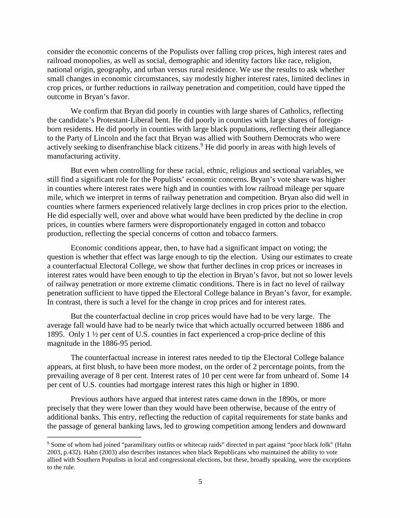
Building on support from both parties, Bryan secured 46.7 percent of ballots cast and 176 electoral votes. Bryan won all electoral votes west of the Mississippi except those of California,

19 See Parker (1972) for more detail on these demands for government intervention. 20 Data are from David Leip's Atlas of United States Presidential Elections, more on which below.

12

Oregon, North Dakota, Iowa and Minnesota (Figure 3).21 He won all Southern states except West Virginia and Kentucky (where he lost by just 277 votes). He did poorly in New England and the Mid-Atlantic and North Central regions.22

These broad strokes are partly explained by traditional sectional divisions. The South had been solidly Democratic since the Civil War, even more so as additional black residents were disenfranchised.23 The West was a natural constituency of the Populist Party due to its dependence on agriculture and mining.24 The Northeast and Middle Atlantic regions, being more urban and industrial, were consistently Republican.

These regional patterns can also be seen through an economic lens. Bryan sought to maximize his advantage in the farm belt, emphasizing free silver as the policy that resonated most strongly with farmers. “Historians have tended to equate the agricultural issue almost exclusively with free silver, partly no doubt because William Jennings Bryan placed the whole farm question in this context…Bryan attempted to tie practically all of the farmers’ woes to an inadequate financial and monetary system” (Fite 1960, p.788). While Bryan also criticized bankers for maintaining interest rates at artificially high levels, and the railways for their discriminatory freight rates, the monetary question was at the heart of his worldview, or at least of his campaign.

This observation in turn points to the question of why Bryan did not attract enough farm votes to win the North Central states.25 Some authors have suggested that agricultural conditions were different in the North Central than further west and south. Farmers in the East North Central states had not been afflicted as severely by drought as farmers in the Great Plains and Mountain regions further west (Durden 1965, p.143). They grew different and more diversified crops, relying less on wheat and more on dairy and other perishable farm products.26 Their specialties, the aforementioned dairying and the corn-hog complex, had not experienced price declines as severe as wheat, and, many of their products being perishable, they were not as dependent on world market conditions (Hofstadter 1969, p.23).

The Republicans blamed low farm prices not on the Crime of ‘73 but on the absence of a tariff adequate to promote urban and industrial income growth. Through that channel, they

21 The races in the Pacific states were close. Bryan lost by 1,922 votes in California, and 2,040 votes in Oregon. 22 David Leip's Atlas of United States Presidential Elections. 23 Kousser (1974) and Jones, Troesken and Walsh (2012) describe the measures, ranging from poll taxes, property requirements, literacy tests and education requirements to simple poll locations and times, used by Southern Democrats to disenfranchise blacks but also sometimes poor whites and immigrants in this period. Northern Republicans actively sought to defend and extend black suffrage, in the South in particular, but their commitment to the cause had atrophied by the 1890s (see Wang 1997). 24 According to Glad (1964, p.144), the Populists “would remain an agrarian movement to the end of its days” despite efforts to use it as a political vehicle by prohibitionists, labor leaders, silver men and single taxers. Fusion between the Democrats and Populists was particularly important for Bryan’s electoral prospects in the South, because to leave the party of white supremacy in the South was to “become a pariah.” Instead of accepting assumptions of white supremacy, however, the Populists sought an understanding with Negroes (Glad 1964, p.157). The electoral success of that understanding is an open question, however (see below). 25 As Fite (1960, p. 805) put it, Bryan’s success “was limited largely to farmers in the western prairies and Great Plains, where periodic droughts and crop failures had combined with low prices to cause intense political irritation and discontent.” 26 Likely for similar reasons, New England farmers gave Bryan a smaller percentage of their ballots than he received from any other rural area (Diamond 1941).

13

argued, there would be sustained demand for the products of the countryside. Republican candidates and their supporters also rejected the view that manipulation of market conditions by bankers, industrialists and railway barons was responsible for the difficulties of farmers and workers. They pointed to the conviction of bankers, industrialists and factory workers that McKinley’s platform of sound money and tariff protection offered the best chance for employment and rising incomes for all. The alliance of South and West supporting Bryan, in this view, was a classic agrarian coalition, while the alliance of the Northeast and North Central supporting McKinley was based on industrial and commercial interests.

Yet another sectional divide arose out of the connection between Civil War pensions and the tariff. Union army veterans and their widows received relatively generous pensions by the standards of the day. By the 1890s, more than half of all elderly native-born men in the North were receiving veterans’ benefits of roughly 30 per cent of average earnings.27 The principal source of funding for those pension payments was the tariff, which accounted for a majority of federal government revenues (the remainder coming mainly from excise taxes). Union army veterans, who resided in the North, understood that the Republicans were the party of high tariffs, which made them, by implication, the party of pensions (Quadagno 1988; Skocpol 1992). Republican politicians, for their part, supported generous pensions precisely because they provided an argument for high tariffs. The rationale for these pension payments, in the view of their critics, was “to cultivate the ‘soldier vote’ for (Republican) party purposes.”28

Others like Glad (1964, p.503) attribute Bryan’s defeat to his failure to secure more votes from workers in industry. The Republican Party agenda, according to Degler (1964, p.44), was “more suited to the needs and character of the new urban, industrial world that was beginning to dominate America.” The Populist Party sought to attract the support of workers in industry, those who Bryan referred to as the “toiling masses,” by arguing that free silver would enhance their employment opportunities through economic growth. In addition, some Populists advocated restricting immigration, speaking to the concerns of urban workers over cheap labor arriving from nontraditional geographic sources. Others proposed public works through which government would create employment directly, an income tax to fund it, and an end to “government by injunction,” meaning court injunctions like that which ended the Pullman strike in 1894 (Durden 1965, p.131).

Many workers in industry were unmoved by these arguments. If farmers were fixated on free silver, the issue was “at best uninteresting…and, at worst, anathema to them” (Degler 1964, p.48). Workers in industry “were interested in ‘the job supply,’ not the money supply” (Sundquist 1983, p.164). They were receptive to Republican warnings that inflation would erode the purchasing power of their wages (Glad 1964, p.204). They were attracted by McKinley’s 27 The Dependent Pension Act of 1890, whose passage coincided with adoption of the McKinley Tariff, made disabled veterans eligible for pensions whether or not their disability was war related. Old age itself was only classified as a disability by the McCumber Act in 1907, but Ransom, Sutch and Williamson (1993) argue that the Pension Office anticipated the 1907 act for applicants who were politically well connected. 28 The quote is from an 1884 edition of the reformist magazine Century, cited in Orloff (1993), p.234. Unfortunately, we lack county-level data with which to test this hypothesis directly. The sample of Union Army veterans extracted by Robert Fogel and colleagues from pension records housed in the National Archives cannot be linked to the 1890 census, original returns from which do not survive. The Special Census of Veterans conducted in 1890 was not enumerated and published by county. It exists in microfilm in the National Archives, but nearly all the schedules for the states of Alabama through Kansas and those for the western half of Kentucky had been destroyed prior to microfilming.

14

“practical agenda for jobs, good wages, and rising prosperity” (Rove 2015, p.368). Most of all, they were attracted by his advocacy of the tariff, which promised protection for industry and, indirectly, for industrial employment. In addition, workers in manufacturing were not infrequently warned by their employers that orders for industrial goods and therefore their employment were contingent on a McKinley victory and the maintenance of tariffs.29 Some employees were summarily fired for voicing their support for Bryan (Steeples and Whitten 1998). Labor leaders like Eugene Debs prominently endorsed Bryan, but the rank and file were said to be swayed by the arguments of their employers (Durden 1965, p.138).

A related dimension of the electoral landscape, as the preceding discussion makes clear, was the rural/urban divide. The cities disproportionately went for McKinley (Diamond 1941).30 Of the 110 U.S. counties with urban populations greater than 25,000, Bryan won only 30. Consistent with emphasis in the literature on sectional factors, 12 of those 30 were in the South. Bryan did even worse in larger cities, securing only 40.6 per cent of the vote in urban centers of at least 45,000 persons. Only 12 of 82 cities with a population above 45,000 went for Bryan, the majority of which were in the South (Degler 1964, p.48). With the cities voting heavily for McKinley, Bryan had to win the rural vote by a large margin in order to carry the key battleground states in the North Central region and elsewhere, which in too many cases he failed to do (Fite 1960, p.804).

Cities were not only more industrial than the countryside but also more cosmopolitan and diverse in the sense of being home to a mix of religions and nationalities, including recent immigrants. Fite (1960, p.805) emphasizes that the rural/urban and agriculture/industry divides were not the same, and that the 1896 contest “was not strictly an agrarian-industrial conflict as has been so often asserted.” Jensen (1971, p.305) links sound money to economic and cultural pluralism of a sort that appealed to urbanites and immigrants, characterizing McKinley as seeking to “sweep the cities and immigrants into an invincible coalition.” McKinley thus called on “farmers, laborers, mechanics, miners, railroad employees, merchants, professional men and representatives of every rank of people” to unite behind his candidacy, observing that “we are all dependent on each other, no matter what our occupations may be. All of us want good times, good wages, good prices, good markets; and then we want good money always.”31

Immigrants (the foreign born comprising 25 per cent of the adult male population in the 1890 census) were less influenced by the “pietistic moralism” espoused by Bryan and were more politically pluralistic, or pragmatic, in the sense of being prepared to switch parties (Jensen 1971, p.304). They voted for an economic program, not for a moralistic program or along party lines. In practice, it is said, they were disproportionately inclined to support McKinley. In contrast, Bryan’s moralistic “redemption through free silver” appealed to natives, Protestants and Evangelicals (Durden 1965 p.149).

29 McKinley had a history of supporting tariffs while the Democrats had generally sought to lower them. The Tariff Act of 1890 which dramatically raised duties is still referred to as the McKinley Tariff, whereas the Democrats when controlling the White House and dominating both houses of Congress in 1894 reduced the prevailing level of rates. 30 The problem was not just limited to the North Central region. Bryan lost Kentucky and Oregon because of McKinley’s overwhelming support in Louisville and Portland, respectively. 31 New York Times, “Tariff Talk at Canton: Candidate McKinley Continues his Financial Straddle” (3 July 1896), http://query.nytimes.com/gst/abstract.html?res=9F01E2D71730E033A25757C0A9619C94679ED7CF&legacy=true.

15

Bryan and the Populists’ position on immigration is difficult to characterize. Glad (1964) observes that such anti-foreigner sentiment as the Populists espoused was directed mainly at British bankers. An exception was Bryan’s attitude toward Asian immigration. Perhaps reflecting his political base in the West, Bryan was an opponent of Chinese and Japanese immigration, questioning the ability of immigrants from these countries to assimilate (Daniels 1966). This opposition to Asian immigration may have informed his attitude toward immigration more generally. Associating foreigners with social problems, in the 1896 campaign he expressed his strong opposition to the “dumping of the criminal classes upon our shore.”32 Some observers took this as a veiled anti-Catholic and anti-new-immigrant comment designed to appeal to the candidate’s old-immigrant, Anglo-Saxon, Evangelical base.

4. Basic Set-Up and Results

To analyze support for Bryan in the 1896 election, we draw on county-level electoral data assembled and standardized by Clubb, Flanigan, and Zingale (1987). A complication is that, rather than listing presidential votes for each candidate, they list total number of presidential votes for each party: Democrats (which means Bryan), Republicans (which means McKinley), and combined third-party candidates (which means Palmer, Levering, Matchett, and Bentley).33 As a result of Bryan’s hybrid candidacy and his two vice presidential running mates (one Populist, one Democrat), the data appear to categorize some votes for Bryan in a handful of states as votes for third-party candidates.34 We therefore use state-level data by candidate to adjust the county-level data. Specifically, we aggregate votes for the “Democrat candidate” and the “third-party candidates” in those states where the county-level data have the third-party candidates significantly outperforming the official state-level statistics tabulated in David Leip's Atlas of United States Presidential Elections.35 Because third-party candidates as a group never received more than 5.6 percent in these additional state-level sources, we aggregate “Democrat” and “third-party” votes in any state where the data list the “third-party” candidates as receiving more than 5.6 percent of the vote. Fortunately, our results are not sensitive to this procedure.36

32 William Jennings Bryan, “Letter Accepting Democratic Nomination,” 9 September 1896, reprinted in Bryan and Bryan (1900, p.359). 33 John Palmer was the National Democrat candidate known for his pro-gold monetary stance. Charles Matchett was the Socialist Labor candidate which fought for more government control and better working conditions. Charles Bentley was the broader National Prohibition party candidate and Joshua Levering was the narrow Prohibition Party candidate, both of whom pushed for prohibition. No single third-party candidate received more than 1 percent of the national vote. 34 In some cases, all of Bryan’s votes go to the third-party candidates, while in others they are split. For example, in Washington, the county-level data report that the “Democrat candidate” received 1.7 percent of the vote, while the “third-party candidates” received 57 percent, yet the official state-level statistics have Bryan with noticeably more than 57 percent, and the third-party candidates with only 1 percent. Conversely, in Alabama, the data report that the “Democrat candidate” received 54 percent and the “third-party candidates” received 17 percent, yet the official statistics have Bryan with 67 percent and the third-party candidates with about 5 percent. 35 State-level voting totals are provided at http://uselectionatlas.org/RESULTS/data.php?year=1896&datatype=national&def=1&f=0&off=0&elect=0. This practice of using Leip’s figures as definitive follows other recent literature. 36 The reason for this insensitivity is the low number of votes for third-party candidates. As a check we replace %Bryanc with %McKinleyc and find the exact opposite results; that is, we find opposite signs on all coefficients. The one exception is the estimated coefficient on the share of Catholics in a county. When we use the unadjusted measure of Bryan’s vote share we obtain a positive and statistically significant coefficient for that variable. That

16

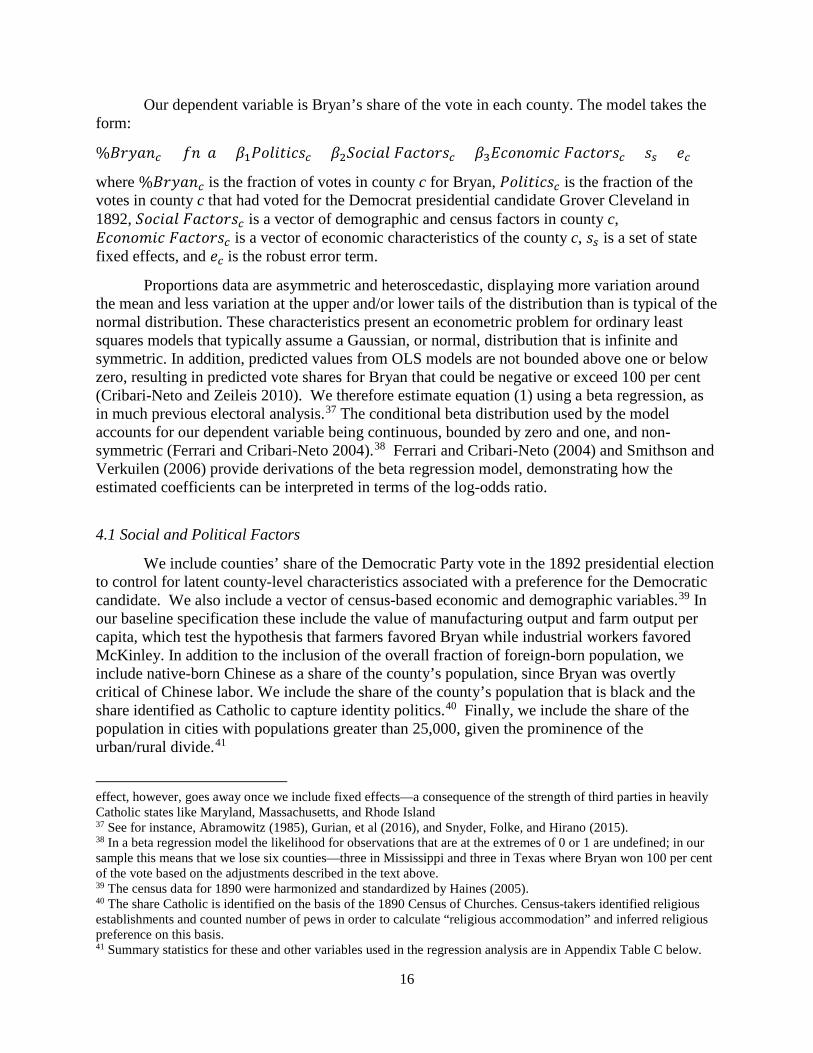
Our dependent variable is Bryan’s share of the vote in each county. The model takes the form:

%𝐵𝐵𝐵𝐵𝐵𝐵𝐵𝐵𝐵𝐵𝑐𝑐 = 𝑓𝑓𝐵𝐵(𝐵𝐵 + 𝛽𝛽1𝑃𝑃𝑃𝑃𝑃𝑃𝑃𝑃𝑃𝑃𝑃𝑃𝑃𝑃𝑃𝑃𝑐𝑐 + 𝛽𝛽2𝑆𝑆𝑃𝑃𝑃𝑃𝑃𝑃𝐵𝐵𝑃𝑃 𝐹𝐹𝐵𝐵𝑃𝑃𝑃𝑃𝑃𝑃𝐵𝐵𝑃𝑃𝑐𝑐 + 𝛽𝛽3𝐸𝐸𝑃𝑃𝑃𝑃𝐵𝐵𝑃𝑃𝐸𝐸𝑃𝑃𝑃𝑃 𝐹𝐹𝐵𝐵𝑃𝑃𝑃𝑃𝑃𝑃𝐵𝐵𝑃𝑃𝑐𝑐 + 𝑃𝑃𝑠𝑠 + 𝑒𝑒𝑐𝑐)

where %𝐵𝐵𝐵𝐵𝐵𝐵𝐵𝐵𝐵𝐵𝑐𝑐 is the fraction of votes in county c for Bryan, 𝑃𝑃𝑃𝑃𝑃𝑃𝑃𝑃𝑃𝑃𝑃𝑃𝑃𝑃𝑃𝑃𝑐𝑐 is the fraction of the votes in county c that had voted for the Democrat presidential candidate Grover Cleveland in 1892, 𝑆𝑆𝑃𝑃𝑃𝑃𝑃𝑃𝐵𝐵𝑃𝑃 𝐹𝐹𝐵𝐵𝑃𝑃𝑃𝑃𝑃𝑃𝐵𝐵𝑃𝑃𝑐𝑐 is a vector of demographic and census factors in county c, 𝐸𝐸𝑃𝑃𝑃𝑃𝐵𝐵𝑃𝑃𝐸𝐸𝑃𝑃𝑃𝑃 𝐹𝐹𝐵𝐵𝑃𝑃𝑃𝑃𝑃𝑃𝐵𝐵𝑃𝑃𝑐𝑐 is a vector of economic characteristics of the county c, 𝑃𝑃𝑠𝑠 is a set of state fixed effects, and 𝑒𝑒𝑐𝑐 is the robust error term.

Proportions data are asymmetric and heteroscedastic, displaying more variation around the mean and less variation at the upper and/or lower tails of the distribution than is typical of the normal distribution. These characteristics present an econometric problem for ordinary least squares models that typically assume a Gaussian, or normal, distribution that is infinite and symmetric. In addition, predicted values from OLS models are not bounded above one or below zero, resulting in predicted vote shares for Bryan that could be negative or exceed 100 per cent (Cribari-Neto and Zeileis 2010). We therefore estimate equation (1) using a beta regression, as in much previous electoral analysis.37 The conditional beta distribution used by the model accounts for our dependent variable being continuous, bounded by zero and one, and non-symmetric (Ferrari and Cribari-Neto 2004).38 Ferrari and Cribari-Neto (2004) and Smithson and Verkuilen (2006) provide derivations of the beta regression model, demonstrating how the estimated coefficients can be interpreted in terms of the log-odds ratio.

4.1 Social and Political Factors

We include counties’ share of the Democratic Party vote in the 1892 presidential election to control for latent county-level characteristics associated with a preference for the Democratic candidate. We also include a vector of census-based economic and demographic variables.39 In our baseline specification these include the value of manufacturing output and farm output per capita, which test the hypothesis that farmers favored Bryan while industrial workers favored McKinley. In addition to the inclusion of the overall fraction of foreign-born population, we include native-born Chinese as a share of the county’s population, since Bryan was overtly critical of Chinese labor. We include the share of the county’s population that is black and the share identified as Catholic to capture identity politics.40 Finally, we include the share of the population in cities with populations greater than 25,000, given the prominence of the urban/rural divide.41

effect, however, goes away once we include fixed effects—a consequence of the strength of third parties in heavily Catholic states like Maryland, Massachusetts, and Rhode Island 37 See for instance, Abramowitz (1985), Gurian, et al (2016), and Snyder, Folke, and Hirano (2015). 38 In a beta regression model the likelihood for observations that are at the extremes of 0 or 1 are undefined; in our sample this means that we lose six counties—three in Mississippi and three in Texas where Bryan won 100 per cent of the vote based on the adjustments described in the text above. 39 The census data for 1890 were harmonized and standardized by Haines (2005). 40 The share Catholic is identified on the basis of the 1890 Census of Churches. Census-takers identified religious establishments and counted number of pews in order to calculate “religious accommodation” and inferred religious preference on this basis. 41 Summary statistics for these and other variables used in the regression analysis are in Appendix Table C below.

17

Column 1 of Table 1 reports a beta regression model of these demographic and political characteristics, where the state fixed effects are excluded. Most of the results are straightforward and intuitive. Support for the Democratic presidential candidate in 1892 is a predictor of Bryan’s success in 1896. Bryan’s share of the vote was lower in counties more reliant on manufacturing. His support was less in counties with a larger share of foreign born population, consistent with the idea that Bryan’s “moralistic piety” did not appeal to immigrants to the same extent as did McKinley’s economic pragmatism. Although Democrats had traditionally been seen as friendlier to Catholics and immigrants, as noted above, this was evidently enough to swing these groups in Bryan’s favor in 1896.42

Bryan’s message regarding the restriction of Chinese labor seems to have resonated with voters, in the sense that his support was higher in counties with larger Chinese populations. The Chinese themselves, of course, did not vote. The 1790 Naturalization Act prevented people of Asian descent from becoming naturalized, while the 1870 Naturalization Act extended citizenship rights to Afro-Americans but not to Chinese, a distinction affirmed by federal courts in 1878 (Torok 1996). The 1882 Chinese Exclusion Act then definitively prohibited Chinese entry and right to vote. The positive coefficient suggests a role for nativism in the 1896 election, although this variable may also be picking up the extent to which Bryan did better than otherwise expected in California, where the Chinese population was concentrated.43 We return to this question momentarily.

There are three unexpected results in column 1. First, Bryan appears to have done better in counties where a relatively large share of the population lived in cities, defined here as centers with a population of at least 25,000, where the literature is unanimous in arguing that McKinley won the cities, aside from those in the South. Second, farm output per capita is not significantly associated with Bryan’s vote share. This is surprising since the Populist Movement originated in and is thought to have derived much of its strength from the Farm Belt. Third, Bryan did significantly better in counties with larger black populations. While Bryan actively courted the black vote (Durden 1965, pp.151, 166-7), this result is inconsistent with the presumption that Bryan alienated black voters by allying with the Southern Populists, with the extent of black disenfranchisement, and with the presumption that blacks retaining the vote remained faithful to the Republican Party.

As a first step in resolving these questions, column 2 appends two additional agricultural factors: the values of the county’s output of cotton and tobacco as a share of total farm output.44 These variables are designed to capture the special concerns of tobacco and cotton farmers described in Section 2. For self-evident reasons, they are correlated with farm output. They are also correlated with the location of the black population. Cotton and tobacco were grown mainly in the South, and counties with large black populations were almost exclusively southern at this time. This also means that they are correlated with the extent of black disenfranchisement, which

42 See our discussion in Section 1 of how in 1896 these patterns deviated from the electoral norm. 43 According to the 1890 Census, 67 per cent of persons listed as born in China were in California. 44 We measure the value of both cotton and tobacco prices using agricultural output data obtained from the 1890 Census of Agriculture (Haines, Fishback and Rhode 2016) weighed by the respective price of cotton and tobacco in 1895 from Carter et al. (2006). These data were assembled from the U.S. National Agricultural Statistics Service (1999) and U.S. Department of Agriculture (various years) by Alan Olmstead and Paul Rhode. The price estimates come from “farmers’ estimates on December 1st of average prices for the season’s sales” (Carter et al. 2006, Notes to Table Daa667-678).

18

was predominantly a southern phenomenon, and with the presumed tendency of white Southern Populists to vote for Bryan.

Both of the new variables enter with positive and statistically significant coefficients, suggesting that agricultural constituencies reliant on cotton or tobacco were more supportive of the Populist candidate, a finding consistent with qualitative accounts. Bryan, it is clear, enjoyed exceptional electoral strength in cotton and tobacco growing regions where farmers had special grievances. Moreover, the addition of the cotton and tobacco measures changes the coefficient on the share of blacks in the population from significantly negative to significantly positive, such that it is now consistent with the predictions of the qualitative literature. To put it another way, outside of the cotton and tobacco growing regions where disenfranchisement was increasing, Bryan received less support from areas with high proportions of black residents.

However, the addition of these crop variables does not resolve the farm output paradox (that the coefficient on farm output is indistinguishable from zero). Nor does it overturn the provisional result that Bryan did better in cities.

Perhaps the positive coefficients on tobacco and cotton output and the negative coefficient on total farm output are all picking up the influence of other state-specific factors, for example the fact that tobacco and cotton grow primarily in the South, an area that had been solidly Democratic since the Civil War. Column 3 therefore adds a vector of state fixed effects to account for this and other unmeasured geographic factors that influenced political preferences in 1896. Those state fixed effects are significant as a group; the standard statistics suggest that they should be included, and we do so in what follows. Tobacco and cotton output remain important as before. But the coefficient on total farm output remains insignificantly different from zero. It would appear that cotton and tobacco farmers had special grievances that shaped their voting behavior. Otherwise, however, the level of farm output was not associated with the Bryan vote. What in fact mattered, as we show below, was the change in the value of that output.

With the inclusion of these fixed effects, the coefficients on the variables measuring urbanization and the size of the Chinese population become statistically insignificant, reflecting the concentration of urban areas in the Northeast states, where McKinley did relatively well, and the Chinese in California, which McKinley won by fewer than 2,000 votes. It does not appear that counties within California where the Chinese population was concentrated voted for Bryan more heavily than other California counties. The change in the coefficient on urban population from positive and significant to insignificantly different from zero places it more in line with the predictions of the qualitative literature (or at least eliminates its prior inconsistency). In contrast, other demographic and economic factors – voting in 1892, manufacturing output, the foreign-born share of the population, and the Catholic share – all retain their expected signs and statistical significance.

4.2 Economic Factors

Table 2 adds economic factors associated with the Populist revolt: changes in crop prices, drought conditions, railroad penetration, and interest rates.

19

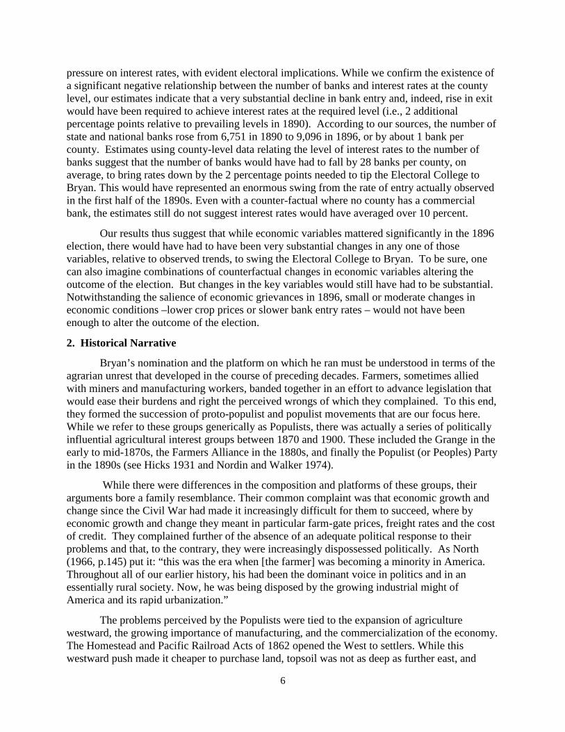
Farmers were upset about long-term trends in prices, this being the implication of their focus on the gold standard and free silver.45 To measure the effect of agricultural price changes, we calculate the percentage change in the value of a fixed basket of a county’s crops between 1886 and 1895.46 The basket consists of the county’s production of corn, barley, oats, wheat, Irish potatoes, sweet potatoes, hay, rye, buckwheat, cotton, and tobacco, as recorded in the 1890 Census of Agriculture (Haines, Fishback, and Rhode 2016), to which we apply the agricultural prices from Carter et al (2006).47 We take the terminal date as 1895 on the grounds that election results, or even expectations in the wake of the nominating conventions, could have affected price developments in 1896, given the price implications of decisions over the future of the gold standard and tariff policy. This provides us with the percentage change in the value of a county’s agricultural basket in the run-up to the 1896 election.

Figure 4 shows the change in the agricultural basket between 1886 and 1895 at the county-level. While all counties experienced a decline in the value of their portfolio, the map shows that the largest falls were concentrated, broadly speaking, in the Midwest, where grains and similar crops predominated, although there are also pronounced falls in Central California, where wheat cultivation predominated. While the South was reliably committed to the Democratic Party, the Midwest was much more in play. The important question, therefore, is whether relative declines within a state lead to more Bryan votes in the election – as we do, in effect, by including state fixed effects in these regressions.

In column 1 of Table 2 we find that the change in the value of a county’s agricultural basket has a negative and statistically significant effect on support for Bryan, a result consistent with historical narratives of the 1896 election. The inclusion of the change in the agricultural basket does not alter the statistical significance of cotton and tobacco as a share of total agricultural output, a result that is again consistent with the qualitative literature.48

45 There is also a revisionist interpretation of rural support for free silver, in which it is argued that in its absence there was a shortage of small-denomination coinage, which created special hardship in under-banked rural areas, resulting in residents there being pushed into the hands of merchants, with whom they were forced to engage in barter transactions and who charged exorbitant rates for credit (Gramm and Gramm 2004). This problem grew especially acute once taxation of their note issuance discouraged state banks from issuing small-denomination notes. While we cannot test this hypothesis about motives for voting directly, we do consider banks per capital and bank per square mile, and find no evidence that these were associated with voting behavior (see below). 46 Our results are robust to considering shorter periods, say the five year period ending in 1895. This longer period has the advantage that our census data on crop mix, from 1890, is from squarely in its middle. It would be convenient to have data in changes in crop mix over time in order to be able to test the hypothesis that substitution opportunities further affected the vote (although this would also introduce index-number problems). In the event, such data are not available. 47 As described in Carter et al. (2006), the price data come from the U.S. National Agricultural Statistics Service (1999) and U.S. Department of Agriculture (various years) with the exception of the price of buckwheat which comes from the U.S. Agricultural Marketing Service (1958). Ideally, we would have information on farm-gate prices at the county level, where here we are using national averages. 48 Retaining these measures of cotton and tobacco production is important for identifying the effect of the change in the value of the overall crop basket because cotton and tobacco producers voted for Bryan in larger numbers than other farmers suffering analogous price declines and because the fall in cotton and tobacco prices was smaller than the fall in a number of other crop prices, as noted above. This fact, together with the disproportionate support of these farmers for Bryan, greatly attenuates the coefficient on the change in the value of the agricultural basket in the absence of these additional variables.

20

As a further measure of agrarian distress, in column 2 we substitute for our measure of the change in crop prices historical weather data from the National Oceanic and Atmospheric Administration (NOAA), which began collecting temperature and weather data in 1895. NOAA provides an index of drought severity based on the Palmer Drought Severity Index (PDSI); this runs from -6 to +6, with values -3 and below indicating a “severe drought.”49 The results suggest that counties hit by severe drought in 1895-6 had lower vote shares for Bryan than counties not so severely affected.

This result is not consistent with the presumption that agrarian distress automatically translated into support for Bryan. This finding is not sensitive to how the severity of drought is measured. When we re-code the NOAA index into a dummy variable that equals one for values of -3 and below, or into a pair of dummy variables for extreme drought and extreme wetness, the result remains unchanged (the coefficient on extreme drought is significantly different from zero and associated with McKinley support, while the coefficient on extreme wetness does not differ significantly from zero). Nor does omitting the state fixed effects result in a positive effect of drought on Bryan’s share of the vote; it does, however, render the coefficient statistically insignificant.

A possible interpretation of this contrary result is that farmers adversely affected by drought were less inclined to attribute their difficulties to the absence of free silver, the argument Bryan emphasized. Another possibility is that farmers suffering the effects of drought blamed the incumbent party (the Democrats) for lack of government support. Finally, it may be that drought not just in 1895-6 but also in earlier years mattered for farm distress and that conditions in earlier years were imperfectly, even negatively, correlated with conditions in 1895-6. Unfortunately we are unable to test this hypothesis, since NOAA began collecting this information only in 1895. Be this as it may, the estimated effect of our other, preferred measure of agricultural distress, the county-specific decline in crop prices, remains essentially unaffected by inclusion or exclusion of this variable, as we show below.

To address concerns about railroad rates, in column 3 we include a measure of railroad penetration in the county, using data from Donaldson and Hornbeck (2016).50 We measure railroad penetration as rail mileage per square mile in a county; this should at least crudely 49 We obtained the Palmer Drought Severity Index (PSDI) data from NOAA’s server at ftp://ftp.ncdc.noaa.gov/pub/data/cirs/climdiv/. The PSDI is measured at a monthly interval and it indicates “the severity of a wet or dry spell. This index is based on the principles of a balance between moisture supply and demand. Man-made changes were not considered in this calculation. The index generally ranges from -6 to +6, with negative values denoting dry spells and positive values indicating wet spells. There are a few values in the magnitude of +7 or -7. PDSI values 0 to -.5 = normal; -0.5 to -1.0 = incipient drought; -1.0 to -2.0 = mild drought; -2.0 to -3.0 = moderate drought; -3.0 to -4.0 = severe drought; and greater than - 4.0 = extreme drought. Similar adjectives are attached to positive values of wet spells. This is a meteorological drought index used to assess the severity of dry or wet spells of weather.” The NOAA starting the data in January of 1895. To construct our measures, we took all months from January 1895 through October 1896—the month before the Presidential election—and coded a drought based on the minimum PSDI value during that period. We are grateful to Mark Seiderman at NOAA’s National Centers for Environmental Information for pointing us to this data and for providing a concordance between NOAA’s climate regions (circa 1895) and county boundaries. 50 Donaldson and Hornbeck (2016) make use of the historical transportation maps digitized and made available by Atack (2016). As detailed in Atack (2013), this database was created by digitizing the locations of transportation options (railroads, canals, and navigable rivers) on highly accurate state-level transportation maps in 1911 and then creating year-specific transportation snapshots by systematically removing sections that were not shown in whatever maps were available for the specified year.

21

capture railway monopoly power. We anticipate that railroad penetration, so measured, will be associated with lower support for Bryan. This is what we find in column 3.51

Some analysts of the 1896 election emphasize that it was not just a contest between manufacturing and agriculture, but that financial interests also played a significant role. Farmers blamed Eastern financiers for high interest rates and for their opposition to free silver (which in their view made for low crop prices). They were unhappy about the high cost of mortgage credit. In column 4, we therefore add a measure of the mortgage interest rates on encumbered farms and homes from U.S. Bureau of the Census (1890).52 The estimates suggest that counties where interest rates were higher, other things equal, voted in larger numbers for Bryan, consistent with qualitative accounts.53

In column 5 we include all the economic factors in a single model.54 Notably, all measures of the Populists’ economic grievances, including crop prices, interest rates, railroad rates, and cotton- and tobacco-market-specific problems, continue to matter as before, as do socioeconomic variables like black and Catholic shares of the population, and structural variables like per capita manufacturing production. Thus, we confirm that not one but a range of economic grievances and concerns influenced voting patterns in 1896, not to the exclusion of structural, sociological and demographic factors but rather in addition to them.55

5. Counterfactuals

As noted previously, Bryan could have won the Electoral College with only 19,436 additional votes. But would a further decline in crop prices, changed drought conditions, increased railway penetration or a slightly higher level of mortgage interest rates have gotten him those votes and tipped the Electoral College balance in his favor?

To answer these questions, we used the model in column 5 of Table 2 to predict the county vote share for Bryan, holding other independent variables at their observed values while varying the variable of interest in fixed increments. For, example, we raise the observed interest rate in all counties in increments of 25 basis points (1/4 of one percentage point) from their

51 Some readers may worry that we neglect alternative modes of transportation (canals and navigable waterways). We would counter that these were not the targets of Populist ire; nonetheless, we return to this question below. 52 The published census volumes provide the value of mortgages as well as interest paid, from which the interest rates were calculated. 53 As an alternative measure of financial conditions, we added various measures of bank penetration and bank failures in each county. Specifically, we included variables measuring the number of state and national banks that failed between 1890 and 1896, both as a raw count and as a share of the total number of banks in existence in 1890, as well as the change in the number of state and national banks during that period for each county. In no specification were these coefficients statistically different from zero at standard confidence levels. Inclusion of these variables did not significantly alter the parameter estimate for the results that we report. We return to the role of bank penetration and entry in Section 5 below. 54 Further, we retain the “identity variables” included in Table 1. A principal components analysis yields four factors with eigenvalues greater than one. The third and fourth principal components are associated with agriculture: they are dominated by cotton output and the change in the value of the crop portfolio, and by tobacco output and total farm output, respectively. The first and second components are associated with combinations of socioeconomic and economic variables but resist easy interpretation. 55 In Appendix A we re-estimate the model in column 5 using fractional probit (‘quasi-probit’) and ordinary least squares. Regardless of the econometric procedure, we get similar results in terms of sign and hypothesis tests for our variables of interest.

22

observed levels until this variable tips the Electoral College. We similarly vary the other key economic variables one by one.

To extract the implications for the Electoral College, we first we calculate the number of votes Bryan would win, conditional on the parameter estimates in column 5 of Table 2.56 We do this by multiplying the total number of votes cast in a county by the fraction of the vote that Bryan wins in that county according to our model. Then, we aggregate Bryan’s predicted county vote total within each state and see if, for each value of the variable interest, Bryan’s number of votes in the state exceeds that of McKinley. If Bryan has a majority, we award him that state’s electoral votes.57 Finally, for each value of the variable of interest, we sum Bryan’s total number of electoral votes and see if the electoral vote total exceeds the 224 vote threshold necessary to win the Presidency. 58 Estimates of Bryan’s electoral fortunes based on our model are consistent, reassuringly, with the outcome in 1896: holding all covariates at their actual values, we predict that Bryan would have won 193 electoral votes, a sum slightly higher than his actual Electoral College tally of 176.59

In Figure 5 we show the counterfactuals as we vary crop prices. The average change in a county’s agricultural basket between 1886 and 1895 is -22 per cent with a minimum of -45 per cent and a maximum of -4.5 per cent. This range is a function of the composition of farm output and the fact that swings in commodity prices varied by crop: between 1886 and 1895 the price of hay increased by 10 per cent while prices of tobacco, corn, wheat, and cotton fell by 6 per cent, 54 per cent, 30 per cent, and 6 per cent respectively. Thus, counties experiencing the largest drops in the value of their agricultural portfolio were those heavily reliant on corn and wheat—counties in the Dakotas, California, and Illinois. At the other end of the spectrum, counties that produced significant quantities of tobacco and cotton—counties in the South and mid-Atlantic—saw the value of their agricultural remain relatively stable over the decade preceding the 1896 presidential contest.

Our counterfactual simulations suggest that a further decline in crop prices could have tipped the outcome of the election. That is to say, there is a set of changes in agricultural portfolio values between 1886 and 1895 that lead to an Electoral College victory for Bryan: a further loss of 20 per cent of the value of a county’s agricultural portfolio on average would net a sufficient number of votes to get Bryan over the top. (The states that shift into Bryan’s column as crop prices are progressively reduced are, in order, South Dakota, Kentucky, Indiana, Oregon,

56 There are approximately 200 counties that have data missing for one or more of the independent variables; consequently, we are unable to generate a predicted vote share for these observations. Rather than dropping those counties, we opt instead to replace the missing values with Bryan’s actual vote share from that county. We note, however, that dropping the counties does not yield different counterfactual results with regard to Bryan’s ability to win sufficient votes for an Electoral College victory. 57 This mechanical application of the winner take all rule means that we miss the defection of two electors—one in California and one in Kentucky, each of whom defected from the rest of that state’s electoral college contingent. 58 We calculate the majority of individual votes needed to win as follows. We assume that Bryan only has to top McKinley’s share and thus toss out all votes for third party candidates. Under this procedure, Bryan does not have to get the majority of total votes but only has to receive more votes than McKinley. In an alternative procedure, which we refer to as the extreme bound, we assume that McKinley received all non-Bryan votes. In this case, Bryan would need 50 percent of all votes in a state to win a majority. We consider this an extreme (upper) bound because it is the fewest votes that assures Bryan will win the state regardless of the success of third-party candidates. 59 We (mis)predict wins for Bryan in California and Kentucky (both states where McKinley won very narrow victories) and a loss for him in Wyoming (where Bryan won a narrow victory).

23

West Virginia, Wyoming, and Ohio.60) Recall that the actual decline in the value of the agricultural portfolio was 22 per cent on average; thus, to tip the balance in Bryan’s favor, the extent of the price decline, so measured, would have had to be almost twice as great as actually observed. This is a big change. Another way of putting it is that only 40 of some 2,000-plus counties actually experienced an average price decline of more than 40 per cent.

For the drought counterfactual we proceed analogously, holding other variables (including railroad penetration and the interest rate) at their actual county means and varying PSDI by ½ point increments (where, recall, -6 indicates severe drought while 6 indicates conditions much wetter than normal).61 There is no level within the range of observed values of drought that yields an Electoral College victory for Bryan; consequently we do not display the results graphically.62

For the railroad counterfactual we vary a county’s level of railroad mileage by increments of 1/20th of a mile. Again, we do not display the results because the elasticity of the Bryan vote share is sufficiently small that no level of railroad mileage generates a level of support necessary for Bryan to carry the Electoral College. Moreover, states with a high density of railway lines, where a very large counterfactual reduction in railway density is feasible, were not, in general, competitive states (generally, McKinley won them by a wide margin). While railroad penetration clearly mattered for voting patterns, it did not matter enough to tip the balance.

We double checked this result in a number of ways. For example, we substituted several alternative measures of railway penetration: railway mileage per capita, the log of total rail mileage in the county, the log of total rail mileage within ten miles of the county, and a dummy variable equaling one when a county has any railway lines. These variables similarly entered with negative coefficients in our basic model, and a number of their coefficients were significantly different from zero at standard confidence levels. But in no case was the coefficient of sufficient size for a different counterfactual value of the variable to tip the Electoral College in Bryan’s favor.

Second, we dropped other variables with which railroad mileage is correlated, since multicollinearity may attenuate the coefficient on railroad mileage. Some readers may suspect that the small size of the coefficient on railroad mileage reflects the fact that certain states, Pennsylvania, Illinois, New York, and Massachusetts for example, had dense networks of railroad track in counties where those railways serviced relatively high levels of manufacturing activity.63 Indeed, this association of manufacturing with the density of railroad mileage attenuates the coefficient on railroad mileage, but dropping manufacturing output from the

60 Duquette, Mixon and Cebua (2017) calculate an “s-factor” for U.S. presidential elections that ranks states by swing-voter influence (the electoral margin between the two candidates divided by the number of winner-take-all Electoral College votes at stake. Reassuringly, the states that swing into Bryan’s column in our counterfactual are high on this list for 1896 (Kentucky first, South Dakota second, Wyoming fourth, Oregon fifth, Indiana sixth, West Virginia thirteenth and Ohio fifteenth). 61 Achen and Bartels (2016) review the literature on when and how voters punish politicians for seemingly random events. 62 We obtain a similar result when we convert the drought index into a dummy variable measuring only severe drought (Palmer index less than or equal to -3). We likewise obtain similar results even if we drop the agricultural variables from the model. 63 The bivariate correlation between railroad mileage per square mile and manufacturing output per capita is 0.56.

24

model, once again, does not alter the outcome of this counterfactual exercise. Similarly, our discussion of Figure 1, above, noted that counties that were home to rail hubs were often disproportionately urban (San Francisco, Portland, Spokane, Denver and Salt Lake City were flagged in that connection).64 Eliminating the urban share of the population does not get Bryan over the Electoral College threshold. Neither does eliminating both the urban and manufacturing shares nor dropping the state fixed effects.65

Third, we added a measure of access to water transport: canals and rivers navigable by steamship (similarly from Atack 2016). We calculated the fraction of a county’s area that is within 10 miles of navigable water.66 Adding this variable as an additional regressor and adding also its interaction with our railway measure do not much change the coefficient on the railway variable, which remains negative and statistically significant at standard confidence levels.67 Nor do these changes put Bryan over the Electoral College hump for any counterfactual value of the railway variable.

In Figure 6 we plot the electoral vote total for Bryan as interest rates vary. Here the results are at least superficially different. Bryan gains the 224 electoral votes required to win the presidency when the interest rates of each county is raised by 2 percentage points, the resulting level corresponding to a nation-wide average of 10 per cent. The states that shift toward Bryan as interest rates are raised are, in order, Indiana, Oregon, Kentucky, Wyoming, Ohio, and West Virginia. An interest rate of 10 per cent is not an absurd level; some 14 per cent of U.S. counties had interest rates of 10 per cent or higher in 1890. Typically, this level is observed in counties with few banks, where lending was instead done by merchants, landowners, and other sources of direct finance unconstrained by usury laws.68 Note, moreover, that such high interest rates were not entirely peculiar to the West. In fact they also occurred in a number of Southern and Eastern counties with the conditions described above.

The question is whether there were plausible developments in financial markets in whose absence interest rates would have been 2 percentage points higher in 1896, thereby tipping the Electoral College in favor of Bryan. Davis (1965), Sylla (1969), and James (1976) note that interest rates declined in the decade leading up to the 1896 election, particularly in Western and Southern regions where they started out high, and especially in rural counties without Central Reserve and Reserve Cities.69 They attribute this decline to the entry of state banks, which intensified competition among lenders and reduced monopoly power in previously uncompetitive markets.

64 The bivariate correlation between railroad mileage per square mile and the urban share of the population is 0.44. 65 When we drop all of the variables in Table 2 expressed in per capita terms (all eight of them, including population living in cities of at least 25,000 as a share of total county population), the negative value of the railroad miles variable triples in size, an increase that gets Bryan over the Electoral College threshold. Arithmetically, this is because railroad miles per square mile and population have a large positive correlation (0.64), making for a significantly larger (in absolute value terms) coefficient on the railway variable when all these regressors are dropped. This, however, is clearly not a well-specified model. We mention the fact only to confirm that there is nothing about the construction of the railway variable or our counterfactual procedure that would in principle prevent changes in the railway variable from tipping the balance. 66 Altering 10 to 5, 15, 30 or 50 changes nothing reported in this paragraph. 67 The coefficient on this variable, like that on railways, is negative, statistically significant and small. 68 We consider the role of usury laws explicitly in the appendix. 69 The downward trend in interest rates slowed in the 1900s and in some regions even began to see rate increases, especially after the Panic of 1907.

25

The list of banks operating in each year in the Rand McNally Bankers Directory indicates that the number of state banks rose from 3,378 in 1890 to 5,396 in 1896, while the number of national banks rose from 3,373 to 3,700.70 Conventional wisdom (e.g. White 1983) is that bank entry, state bank entry in particular, was driven by the rise of deposit banking (in which state banks were pioneers because of prohibitive taxes on the alternative source of funding, namely note issuance), the lowering of deposit reserve and minimum capital requirements, and the simplification of incorporation laws.71 White (p. 2010, p.1) writes of active “competition of laxity” in this period, as states seeking to increase the number of banks within their borders relaxed restrictive banking legislation. It is not unreasonable to infer that a number of states lowered capital requirements and simplified incorporation laws in response to complaints by Populists and others that lack of bank entry and competition in the earlier period heightened monopoly power, not to mention interest rates themselves. James (1976, p. 897) argues that bank entry was responsible for narrowing regional interest rate differentials and, specifically, for reducing rates where they were high. He concludes that "(l)ower capital requirements, more liberal regulations, and, after the 1880's, the passage of general banking laws which made incorporation much easier encouraged the formation of state banks rather than of national banks. These institutions were primarily responsible for breaking down local monopolies." In our county-level cross-section, the correlation between the total number of banks and interest rates is -0.23, consistent with this interpretation. To delve further into this relationship, we ran simple regressions relating the level of interest rates in 1890 to the number of banks in that county and a vector of state-level regulatory variables (capital requirements, usury rates, and indicators of the presence or absence of reserve requirements and double-liability laws). The elasticity of interest rates with respect to the number of banks is -0.07 and significantly different from zero at standard confidence levels.72 This point estimate suggests that bank entry in the 1890s or even the late 1880s was not large enough to lower interest rates by 2 percentage points and tip the scales away from Bryan. As noted above, our sources indicate that the number of state and national banks rose from 6,751 in 1890 to 9,096 in 1896, or about 1 bank per county. Even if that entire growth had not occurred, interest rates would have still been low enough to elect McKinley. The point estimate of -0.07 implies that there would have to be 28 fewer banks per county to lead to such a substantial rise in interest rates that would hand Bryan the victory. This is a tall order. Less than 1 per cent of U.S. counties had more than 28 banks and 40 per cent of all counties did not have a single bank. Therefore, even in a counter-factual where every county had 0 commercial banks, the model predicts that average interest rates would have been below 10 per cent. These facts in turn suggest that even moderately sized increases in the posited elasticity of interest rates with respect to bank entry would not alter the election.73

6. Conclusion

70 The capital of state banks rose by 46.2 per cent over the period, that of national banks by 5 per cent. 71 Fohlin and Jaremski (2015) also find a role for economic growth, which improved after 1893, in creating new lending opportunities. 72 Regression results are reported in Appendix Table B. 73 Nor would changes in other factors affecting interest rates, such as usury restrictions. See the appendix.

26

The 1896 presidential race between Bryan and McKinley is an iconic episode in American history, one with new resonance in the wake of the 2016 election. The 1896 campaign had a prominent urban-versus-rural dimension. It arrayed those invested in what had traditionally been important economic sectors and activities, sectors and activities whose share in GDP were in decline, against others whose interests were aligned with newly important, expanding sectors. Voters were divided by race and religion. There were divisions between the “heartland” and the Northeast. Most controversially, the election revolved around economic issues. It featured an array of economic complaints from farmers and others focusing on low crop prices, high interest rates and unfair freight rates. And the outcome, a McKinley victory, essentially set the course of U.S. economic policy for a generation.

But earlier studies provide little guidance on the quantitative importance of these factors, and of these economic variables in particular, in the electoral outcome. We know that the election was closely fought, but until now scholars have had little sense of whether changes in economic conditions – less favorable crop prices, higher mortgage interest rates, less freight-rate competition, more extreme climatic conditions – could have tipped the Electoral College balance in Bryan’s favor, notwithstanding suggestions that McKinley owed his victory to improving economic conditions.

Our estimates and counterfactuals suggest that further declines in crop prices and higher mortgage interest rates, but not still lower levels of railway penetration and competition, could in principle have tipped the Electoral College balance. While railway penetration mattered for voting patterns, its effect was quantitatively small, and there was no level of rail-line density low enough to shift the Electoral College in Bryan’s favor.

In contrast, had gold not been discovered in South Africa in the 1880s and in Western Australia in the early 1890s and had the cyanide process for separating gold and impurities not been developed, agricultural prices might have continued to fall rather than rising, in which case the outcome of the election could indeed have been different.74 Our estimates suggest, however, that this further fall in prices would have had to have been very substantial for Bryan to win enough electors to capture the presidency. Similarly, our estimates suggest that even if none of the bank entry actually observed in the first half of the 1890s had occurred, resulting in a higher level of interest rates, that increased level would still not have been enough to swing the election toward Bryan.

One can also imagine a combination of counterfactual changes in economic variables altering the outcome of the election. We show one of those combinations in Figure 7: a one percentage point increase in interest rates relative to prevailing levels, combined with an additional 10 per cent decline in crop prices.75 The requisite changes remain substantial. Crop prices still would have had to fall half again as fast as they in fact did in the decade preceding the election. Fourteen fewer banks per county, as needed to raise the level of interest rates by one percentage point on average, is still a large multiple of the observed rate of bank entry between 1890 and 1896. There is no question that economic grievances were salient. But a small or even

74 Friedman (1992) and Bordo and Redish (2004) discuss the impact of these gold discoveries on trends in the price-level. 75 Since the models estimated in Table 2 are linear, this new counterfactual is essentially a linear combination of the counterfactuals in the two preceding figures, where the requisite fall in crop prices, taken in isolation, was 20 per cent, and the necessary rise in interest rates, taken in isolation, was 2 percentage points.

27

moderate change in economic conditions would not have altered the outcome of the 1896 election.

28

Appendix: Interest Rate Regressions

In this appendix we report the regressions used in Section 5 to discuss the determinants of interest rates in 1890, particularly the effect of bank entry. Data on interest rates on mortgages on farms and homes, taken from the U.S. Census as described in Section 4, are regressed on the number of banks, as tabulated in the Rand McNally Bankers Directory; both variables are at the county level, and both are for 1890. We include in addition a vector of state-level regulatory variables: minimum capital requirements, an indicator of the height of usury-law restrictions, and dummy variables for whether bank stockholders were subject to double liability and whether the state instituted reserve requirements on deposits. Information on minimum capital, in thousands of dollars, is again from the Rand McNally Bankers Directory.76 Double liability is from Mitchener and Jaremski (2015), while reserve requirements are from Rodkey (1934).77 The usury restrictions variable, from Holmes (1892) as digitized by Rockoff (2009), is specified as the highest interest rate allowed in the state, top coded at 25 per cent. The mean of the resulting variable is 10 per cent.

Since the regulatory variables are state-specific, we estimate robust standard errors with observations adjusted for clustering at the state level. In column 1 of Appendix Table B, we regress interest rates on number of banks (state and national alike). While statistically significant, the effect of the number of banks is not particularly large. Because interest rates are in percentage point terms, the 0.07 coefficient on total banks implies that for each additional bank a county’s interest rate would be reduced by 0.07 percentage points.

In column 2 we substitute the number of state banks for the number of total banks, because that is where most of the action was in terms of bank entry in this period, and because state banks dominated the mortgage lending that was of such concern to the Populists.78 The coefficient on number of state banks is larger in absolute value as one would expect, but is not statistically different from the coefficient on the number of all banks. Even so, the larger coefficient suggests that 10 fewer state banks would have been required to raise interest rates by two percentage points, a threshold surpassed by only 8 counties in entire country between 1890 and 1896.

The regulatory variables matter as well. Consistent with previous work on usury legislation by Eichengreen (1984) and Benmelech and Moskowitz (2010), interest rates are positively related to the maximum amount of interest a bank could legally charge on a loan. The coefficient on the usury rate implies that for every 1 percentage point the rate was increased the average interest rates would increase by roughly 0.19 percentage points. To put it another way, interest rates were roughly 3 percentage points higher in states without usury restrictions (top-coded at 0.25) than in the typical usury-law jurisdiction (0.10). A number of states reduced their usury ceilings in the 1889-1895 period, which would have worked to Bryan’s disfavor, according 76 Because many states did not set universal minimum capital requirements across all banks and many others set different requirements for state commercial banks, trust companies, and savings banks, this variable is measured as the capital level of the bank with the minimum capital operating in the state in 1890. This can be thought of as the binding minimum capital requirement in the state. This variable runs from 0 to 150. 77 National banks were also required to hold reserves against deposits, but these requirements did not distinguish between demand deposits and time deposits and did not vary across states. 78 State banks include state commercial banks, trust companies, and savings banks as they all did banking business during the period. National banks were limited to lending on property no more than 25 per cent of their paid-up capital, and no loan could exceed 50 per cent of the appraised value of the land.

29

to our model. Illinois, Iowa, Michigan, Missouri, South Carolina and Texas all reduced their usury rates by 1 or 2 percentage points.79 A point estimate of 0.19 suggests that a 2 point reduction in the ceiling would have reduced observed mortgage rates by 0.4 percentage point, too little to swing the electoral balance.

The double-liability dummy indicates states where shareholders in state banks were at risk of losing more than the initial purchase price of their shares. The negative coefficient on this variable is consistent with the presumption that double liability made stockholders more vigilant about risk and led to bank made safer loans at lower interest rates (as independently shown by Grossman 2001).80 The dummy variable for the existence of reserve requirements on deposits suggests that these were an additional cost of doing business that, by making funding more expensive, were associated with higher interest rates. A number of additional states imposed reserve requirements on deposits in the 1890s, but as late as 1895 fully 31 states and territories still had no such requirements (White, 1883, p.28). Had additional states adopted reserve requirements on deposits, our estimates suggest, their interest rates would have been higher. But our point estimate of 0.33 on this variable suggests that they would have been only a third of a percentage point higher, far short of the two percentage point increase needed to tip the Electoral College in Bryan’s favor.

All the above is as expected. In contrast, the coefficient on minimum capital enters negatively, which is the opposite of what one many readers will expect. They will expect that where the amount of capital required to operate a bank was high, entry would have been slow, resulting in high interest rates. But to the extent that we are already controlling for bank entry by including number of banks, this variable may only be capturing other channels through which capital requirements affected interest rates. Still, to the extent that these other channels constituted additional costs of doing business, one would still anticipate a positive coefficient.

Our results for the 1890s are different because capital requirements in this period were different. Capital requirements were defined as an absolute number of dollars (depending on state- or national-bank status, state of charter and city size), not in relation to assets or liabilities. Thus, banks were free to raise their lending and leverage in response to higher capital requirements, which they in fact did, as Gao (2017) shows. This implies that higher capital requirements in this period had no necessary impact on the cost of credit.81

These facts can explain the absence of a positive coefficient on capital requirements but not a significant negative sign. The negative sign could conceivably reflect populist pressure for low chartering costs where interest rates were high. However, instrumenting this variable with an

79 Illinois went from 8 to 7 percent. Iowa, Michigan, Missouri, and South Carolina went from 10 to 8 percent. Texas went from 12 to 10 percent. 80 This does not mean, of course, that farmers would have been happier as a result, since the mechanism could have been that high-risk borrowers were rationed out of the bank market. One might make the same observation about usury restrictions. 81 Consistent with this, and with the positive response of lending to capital requirements, both Gao (2017) and Jorda, Richter, Schularick and Taylor (2017) do not find a negative association of capital requirements with failure rates in this period.

30

unweighted average of capital requirements in bordering states, on the grounds that states competed for banking business, following Benmelech and Moskowitz, does not alter the result.82

Rather, it appears that this coefficient is driven by outliers with exceptionally high values for both required capital and the usury ceiling. Utah is the extreme case, with the highest minimum capital requirement of any state and a top-coded value of 25 for the usury ceiling. When we drop the usury ceiling, as in columns 7 and 8, capital requirements enter positively and significantly (as would be anticipated from the literature), and the coefficients on the other variables, including number of banks, remain unchanged. When we instead drop the capital variable out of the regression, the key results are again unchanged.

82 Nor does the result change when we substitute minimum statutory capital requirements in 1895 (the first year for which we have information on this variable, courtesy of the annual report of the Comptroller of the Currency) for observed minimum capital (despite the fact that the sample is somewhat smaller owing to missing observations). Reassuringly, the 1895 values of observed minimum capital in 1895 and statutory minimum capital in 1895 are highly correlated. The correlation is highest for states with a relatively large number of banks.

31

References

Abramowitz, Alan (1985). "Economic Conditions, Presidential Popularity, and Voting Behavior in Midterm Congressional Elections," The Journal of Politics 47(1)31-43.

Achen, Christopher and Larry Bartels (2016). Democracy for Realists: Why Elections Do Not Produce Responsive Government, Princeton: Princeton University Press.

Aldrich, Mark (1980). "A Note on Railroad Rates and the Populist Uprising." Agricultural History 54: 424-432.

Atack, Jeremy (2013). “On the Use of Geographic Information Systems in Economic History: The American Transportation Revolution Revisited.” Journal of Economic History 73: 313-338.

Atack, Jeremy (2016). “Historical Geographic Information Systems (GIS) Database of U.S. Railroads for Selected Years”. Available https://my.vanderbilt.edu/jeremyatack/data-downloads/.

Balke, Nathan and Robert Gordon (1989). “The Estimation of Prewar GNP: Methodology and New Evidence.” Journal of Political Economy 97: 38-92.

Barnes, James (1947). “Myths of the Bryan Campaign.” Mississippi Valley Historical Review 34: 383-394.

Benmelech, Efraim and Todd Moskowitz (2010). “The Political Economy of Financial Regulation: Evidence from U.S. State Usury Laws in the 19th Century.” Journal of Finance 65: 1029-1073.

Bodenhorn, Howard (1995). "A More Perfect Union: Regional Interest Rates in the United States, 1880-1960." In Anglo-American Financial Systems: Institutions and Markets in the Twentieth Century edited by Michael Bordo and Richard Sylla, Burr Ridge, Illinois: Irwin Professional Publishers, pp.415-453..

Bordo, Michael and Angela Redish (2004). “Is Deflation Depressing? Evidence from the Classical Gold Standard.” In Richard Burdekin and Pierre Siklos eds, Deflation: Current and Historical Perspectives, Cambridge: Cambridge University Press, pp.191-217.

Bowman, John (1965). "Economic Analysis of Midwestern Farm Land Values and Farm Land Income, 1860 to 1900." Yale Economic Essays 5: 317-52.

Bowman, John, and Richard Keehn (1974). "Agricultural Terms of Trade in Four Midwestern States, 1870-1900." Journal of Economic History 34: 592-609.

Bryan, William Jennings and Mary Baird Bryan (1900). Life and Speeches of Hon. Wm. Jennings Bryan. Baltimore: R.H. Woodward Company.

Burnham, Walter Dean (1965). “The Changing Shape of the American Political Universe.” American Political Science Review 59: 7-28.

Burnham, Walter Dean (1986) “Periodization Schemes and ‘Party Systems’: The ‘System of 1896’ as a Case in Point.” Social Science History 10 (1986), pp.263-313.

32

Bryan, William Jennings (1896). The First Battle: A Story of the Campaign of 1896, Chicago: W.B. Conkey Company.

Calomiris, Charles and Gary Gorton (1991). "The Origins of Banking Panics: Models, Facts, and Bank Regulation." In Financial Markets and Financial Crises, edited by R. Glenn Hubbard. Chicago: University of Chicago Press, pp. 109-174.

Campbell, Tracy (1993), The Politics of Despair: Power and Resistance in the Tobacco Wars. Lexington: University of Kentucky Press.

Carter, Susan, Scott Carter, Michael Haines, et al. (2006). Historical Statistics of the United States: Earliest Times to the Present, Millennial Edition. New York: Cambridge University Press.

Clubb, Jerome M., William H. Flanigan, and Nancy H. Zingale (1987). “Electoral Data for Counties in the United States: Presidential and Congressional Races, 1840-1972,” ICPSR08611-v1. Ann Arbor, MI: Inter-university Consortium for Political and Social Research, 2006-11-13. http://doi.org/10.3886/ICPSR08611.v1

Cribari-Neto, Francisco and Achim Zeileis (2010). “Beta Regression in R.” Journal of Statistical Software 34:1-24

Daniels, Roger (1966). “William Jennings Bryan and the Japanese.” Southern California Quarterly 48, pp.227-240.

Davis, Lance (1965). “The Investment Market, 1870-1014: The Evolution of a National Market.” Journal of Economic History 25: 373-387.

Degler, Carl (1964). “American Political Parties and the Rise of the City: An Interpretation.” Journal of American History 51, pp.41-60.

Diamond, William (1941). “Urban and Rural Voting in 1896.” American Historical Review 46, pp.281-305.Donaldson, Dave, and Richard Hornbeck (2016). "Railroads and American Economic Growth: A ‘Market Access’ Approach." Quarterly Journal of Economics 131: pp. 799-858.

Duquette, Christopher, Franklin Mixon and Richard Cebua (2017), “Swing States, the Winner-Take-all Electoral College and Fiscal Federalism,” Atlantic Economic Journal 45, pp.45-57.

Durden, Robert (1965). The Climax of Populism: The Election of 1896. Lexington: University of Kentucky Press.

Eichengreen, Barry (1984). “Mortgage Interest Rates in the Populist Era.” American Economic Review 74: 995-1015.

Farmer, Hallie (1924). “The Economic Background of Frontier Populism.” Mississippi Valley Historical Review 10: 406-427.

Faulkner, Harold (1959). Politics, Reform and Expansion 1890-1900. New York: Harper.

Ferrari, Silvia, and Francisco Cribari-Neto F (2004). “Beta Regression for Modelling Rates and Proportions.” Journal of Applied Statistics 31: 799–815.

33

Fite, Gilbert (1960). “Republican Strategy and the Farm Vote in the Presidential Campaign of 1896,” American Historical Review 65: 787-806.

Fohlin, Caroline and Matthew Jaremski (2015). “Bank Concentration in the United States, 1800-1914.” Unpublished manuscript, Emory University and Colgate University (December).

Frieden, Jeffry (1997). "Monetary Populism in Nineteenth-Century America: An Open Economy Interpretation." Journal of Economic History 57: 367-395.

Friedman, Milton. 1992. Money Mischief: Episodes in Monetary History. New York: Harcourt Brace Jovanovich.

Frum, David (2016). “The Trump before Trump,” Wall Street Journal (29 July), https://www.wsj.com/articles/the-trump-before-trump-1468607827

Gou, Michael (2017). “Did Capital Requirements Promote Bank Stability in the Early 20th Century United States.” unpublished, UC Irvine.

Glad, Paul (1964). McKinley, Bryan and the People, Philadelphia: J.B. Lippincott Company.

Gramm, Marshall and Phil Gramm (2004). “The Free Silver Movement in America: A Reinterpretation.” Journal of Economic History 64: 1108-1129.

Grossman, Richard (2001). “Double Liability and Bank Risk Taking.” Journal of Money, Credit and Banking 33: 143-159.

Gurian, Paul-Henri, Nathan Burroughs, Lonna Rae Atkeson, Damon Cann, and Audrey Haynes. (2016). “National Party Divisions and Divisive State Primaries in US Presidential Elections, 1948-2012,” Political Behavior 38(3)689-711.

Hahn, Steven (2003). A Nation Under our Feet: Black Political Struggles in the Rural South from Slavery to the Great Migration, Cambridge, Mass.: The Belknap Press of Harvard University Press.

Haines, Michael (2005). “Historical, Demographic, Economic, and Social Data: The United States, 1790-2002,” ICPSR02896-v3. Ann Arbor, MI: Inter-university Consortium for Political and Social Research, 2010-05-21. http://doi.org/10.3886/ICPSR02896.v3

Haines, Michael R., Price Fishback, and Paul Rhode (2016). “United States Agricultural Data, 1840-2012.” ICPSR 3520635206-v3. Ann Arbor, MI: Inter-university Consortium for Political and Social Research, 2016-06-29. https://doi.org/10.3886/ICPSR35206.v3.

Halcoussis, Dennis (1996). "Economic Losses due to Forecasting Error and the US Populist Movement." Economic Inquiry 34: 260-275.

Hicks, John (1931). Populist Revolt: A History of the Farmers’ Alliance and the People’s Party, Minneapolis: University of Minnesota Press.

Hofstadter, Richard (1969). “North America,” in Ghita Ionescu and Ernest Gellner (eds), Populism: Its Meaning and National Characteristics, 9-27. New York: Macmillan Company.

34

Holmes, George (1892). “Usury in Law, in Practice and in Psychology.” Political Science Quarterly 7: 431-467.

Inglehart, Ronald and Pippa Norris (2016). “Trump, Brexit, and the Rise of Populism: Economic Have-Nots and Cultural Backlash,” unpublished manuscript, University of Michigan and Harvard University.

James, John A. (1976). "Banking Market Structure, Risk, and the Pattern of Local Interest Rates in the United States, 1893-1911." Review of Economics and Statistics 58: 453-462.

Jaremski, Matthew, and Price V. Fishback. (2017). “Did Inequality in Farm Sizes Lead to Suppression of Banking and Credit in the Late Nineteenth Century?” Forthcoming in Journal of Economic History.

Jensen, Richard (1971). The Winning of the Midwest: Social and Political Conflict, 1888-1896. Chicago: University of Chicago Press.

Jones, Daniel, Werner Troesken and Randall Walsh (2012). “A Poll Tax by Any Other Name: The Political Economy of Disenfranchisement.” NBER Working Paper no.18612 (December).

Jorda, Oscar, Bjorn Richter, Moritz Schularick and Alan Taylor (2017). “Bank Capital Redux: Solvency, Liquidity and Crisis.” Unpublished manuscript, University of California, Davis and University of Bonn.

Key, V.O., Jr. (1955). “A Theory of Critical Elections.” Journal of Politics 17: 3-18.

Klepper, Robert (1978). The Economic Bases for Agrarian Protest Movements in the United States 1870-1900. New York: Arno Press.

Kousser, J. Morgan (1973). The Shaping of Southern Politics: Suffrage Restriction and the Establishment of the One-Party South, 1880-1910. New Haven: Yale University Press.

Lee, Tom (2014), “Southern Appalachia’s Nineteenth-Century Bright Tobacco Boom: Industrialization, Urbanization, and the Culture of Tobacco,” Agricultural History 88, pp.175-206.

Leip, David (2017). David Leip’s Atlas of U.S. Presidential Elections. http://www.uselectionatlas.org.

MacAvoy, Paul (1965). The Economic Effects of Regulation: The Trunk-line Railroad Cartels and the Interstate Commerce Commission Before 1900. Cambridge: MIT Press.

Macune, C.W. (1891). "The Purposes of the Farmers' Alliance," in N.A. Dunning (ed.), Farmers' Alliance History and Agricultural Digest. Washington, DC: Alliance Publishing Co..

Magliari, Michael (1989). "Populism, Steamboats, and the Octopus: Transportation Rates and Monopoly in California's Wheat Regions, 1890-1896." Pacific Historical Review: 449-469.

Mayhew, Anne (1974). “”A Reappraisal of the Causes of Farm Protest in the U.S., 1870-1900.” Journal of Economic History 32: 464-475.

35

Mayhew, David (2002). Electoral Realignments: A Critique of an American Genre. New Haven: Yale University Press.

McGuire, Robert (1981). "Economic Causes of Late-Nineteenth Century Agrarian Unrest: New Evidence." Journal of Economic History 41: 835-52.

McMath, Robert, Jr. (1993). American Populism: A Social History 1877-1898. New York: Hill and Wang.

Minnesota Population Center (2004). National Historical Geographic Information System: Pre-release Version 0.1. Minneapolis, MN: University of Minnesota. http://www.nhgis.org.

Mitchener, Kris and Matthew Jaremski (2015). “The Evolution of Bank Supervisory Institutions: Evidence from U.S. States.” Journal of Economic History 75: 819-859.

Nordin, Sven and Bertrand Walker (1974). Rich Harvest: A History of the Grange, Jackson, Miss.: University Press of Mississippi.

North, Douglass (1966). Growth and Welfare in the American Past. Englewood Cliffs, N.J: Prentice-Hall, Inc.

Olmstead, Alan and Paul Rhode (2008). Creating Abundance: Biological Innovation and American Agricultural Development. Cambridge: Cambridge University Press.

Orloff, Anne Shola (1993). The Politics of Pensions: A Comparative Analysis of Britain, Canada, and the United States, 1880-1940. Madison: University of Wisconsin Press.

Parker, William (1972). "Agriculture," in Lance E. Davis, et al., American Economic Growth: An Economist's History of the United States. New York: Harper & Row.

Porter, Robert (1983). “A Study of Cartel Stability: The Joint Executive Committee, 1880-1886.” Bell Journal of Economics 14: 301-314.

Quadano, Jill (1988). The Transformation of Old Age Security: Class and Politics in the American Welfare State. Chicago: University of Chicago Press.

Rodkey, Robert Gordon (1934). “Legal Reserve in American Banking.” Michigan Business Studies VI, no.5, Ann Arbor: University of Michigan, Bureau of Business Research.

Ransom, Roger and Richard Sutch (1977). One King of Freedom: The Economic Consequences of Emancipation. New York: Cambridge University Press.

Ransom, Roger, Richard Sutch and Samuel Williamson (1993). “Protecting Soldiers and Republicans: Civil War Pensions, the Protective Tariff and the Failure of the Social Insurance Movement in the Progressive Era,” Working Paper on the History of Retirement no. 5, Institute of Business and Economic Research, University of California, Berkeley (October).

Rockoff, Hugh. (2009) “Prodigals and projecture: An economic history of usury laws in the United States from colonial times to 1900”. In Eltis, David, Frank D. Lewis and Kenneth L. Sokoloff (eds.), Human Capital and Institutions: A Long-run View. New York: Cambridge University Press.

36

Rove, Karl (2015). The Triumph of William McKinley, New York: Simon and Schuster.

Schattschneider, Elmer Eric (1956). “United States: The Functional Approach to Party Government,” in Sigmund Neumann ed., Modern Political Parties: Approaches to Comparative Politics, Chicago: University of Chicago Press, pp.194-215.

Schattschneider, Elmer Eric (1960). The Semisovereign People: A Realist’s View of Democracy in America. New York: Holt, Rinehart and Winston.

Skocpol, Theda (1992). Protecting Soldiers and Mothers: The Political Origins of Social Policy in the United States. Cambridge, Mass: Belknap Press of Harvard University Press.

Shannon, Fred A. (1968). The Farmers Last Frontier. New York: Harper & Row.

Smithson, Michael and Jay Verkuilen. (2006). “A Better Lemon Squeezer? Maximum-Likelihood Regression with Beta-Distributed Dependent Variables”. Psychological Methods 11: 54–71.

Snowden, Kenneth (2010). “Covered Farm Mortgage Bonds in the Late Nineteenth Century U.S.” NBER Working Paper no.16242 (July).

Snyder, J., Folke, O., & Hirano, S. (2015). “Partisan Imbalance in Regression Discontinuity Studies Based on Electoral Thresholds.” Political Science Research and Methods 3: 169-186.

Sprague, O.M.W. (1910). History of Crises under the National Banking System. Washington, DC: National Monetary Commission, Senate Document 538, 61st Congress, 2d Session.

Steeples, Douglas and David Whitten (1998). Democracy in Desperation: The Depression of 1893. Westport, CT: Greenwood Press.

Sundquist, James (1983). Dynamics of the Party System: Alignment and Realignment of Political Parties. Washington, D.C.: The Brookings Institution.

Sylla, Richard (1969). “Federal Policy, Banking Market Structure, and Capital Mobilization in the United States, 1863-1913.” Journal of Economic History 29: 657-686.

Torok, John Hayakawa (1996). “Reconstruction and Racial Nativism: Chinese Immigrants and the Debates on the Thirteenth, Fourteenth and Fifteenth Amendments and Civil Rights Laws.” Asian American Law Journal at Berkeley Law 3: 55-103.

Ulen, Thomas (1980). “Cartels and Regulation: Late Nineteenth-Century Railroad Collusion and the Creation of the Interstate Commerce Commission.” Journal of Economic History 40:179-181.

U.S. Agricultural Marketing Service (1958). Rice, Popcorn, and Buckwheat Acreage, Yield, Production, Price and Value, 1866-1953. Washington, D.C.: Government Printing Office.

U.S. Bureau of Agriculture (Various years). Agricultural Statistics. Washington, D.C.: Government Printing Office.

37

U.S. Bureau of the Census (1896). Eleventh Decennial Census of the United States, (1890). Vol. XIII. Report on Farms and Homes: Proprietorship and Indebtedness in the United States. Washington, D.C.: Government Printing Office.

U.S. National Agricultural Statistics Service (1999), Track Records: United States Crop Production. Washington, D.C.: Government Printing Office.

Wang, Xi (1997). The Trial of Democracy: Black Suffrage and Northern Republicans, 1860-1910. Athens, Georgia: University of Georgia Press.

White, Eugene (1983). The Regulation and Reform of the American Banking System, 1900-1929. Princeton: Princeton University Press.

White, Eugene (2010). “To Establish More Effective Bank Supervision: How the Birth of the

Federal Reserve Altered Bank Supervision.” Paper presented to the Federal Reserve Bank of Atlanta Conference, Return to Jeckyll Island (5 November).

Wicker, Elmus (2000). Banking Panics of the Gilded Age. Cambridge, UK: Cambridge University Press.

Williams, Wayne (1936). William Jennings Bryan, New York: G.P. Putnam’s Sons.

Woest, Victoria Saker (1998), The Farmer’s Benevolent Trust: Law and Agricultural Cooperation in Industrial America 1865-1945, Chapel Hill: University of North Carolina Press.

Woodman, Harold ((1968). King Cotton and His Retainers: Financing and Marketing the Cotton Crop of the South, 1800-1925. Lexington: University of Kentucky Press.

Wright, Gavin (1986), Old South, New South: Revolutions in the Southern Economy since the Civil War, New York: Basic Books.

Wright, Gavin (1990). “The Origins of America’s Industrial Success.” American Economic Review 80: 651-668.

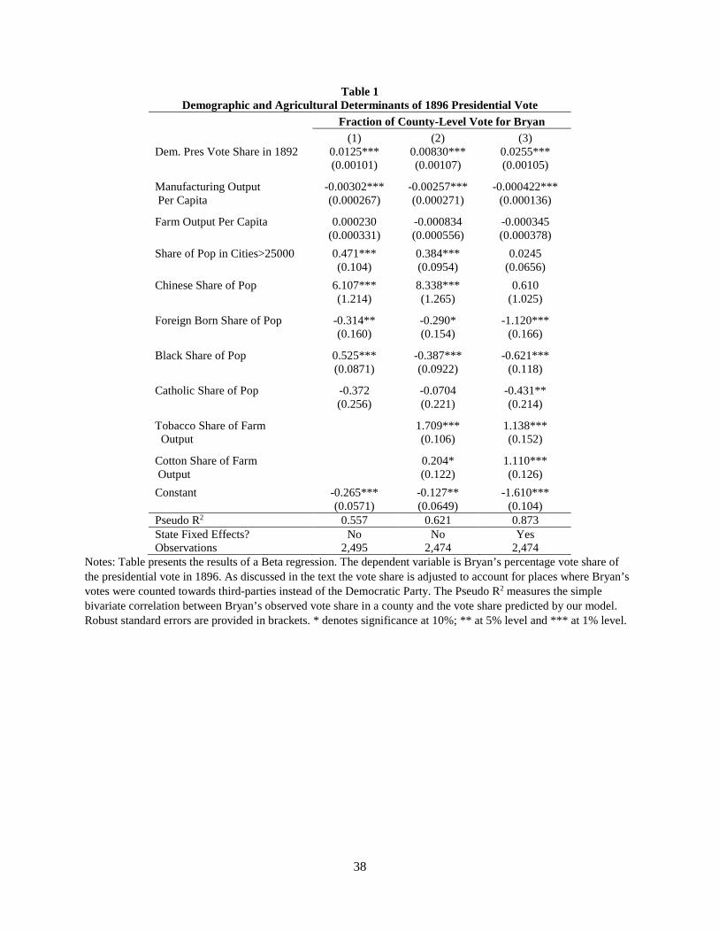
38

Table 1 Demographic and Agricultural Determinants of 1896 Presidential Vote

Fraction of County-Level Vote for Bryan (1) (2) (3) Dem. Pres Vote Share in 1892 0.0125*** 0.00830*** 0.0255*** (0.00101) (0.00107) (0.00105) Manufacturing Output -0.00302*** -0.00257*** -0.000422*** Per Capita (0.000267) (0.000271) (0.000136) Farm Output Per Capita 0.000230 -0.000834 -0.000345 (0.000331) (0.000556) (0.000378) Share of Pop in Cities>25000 0.471*** 0.384*** 0.0245 (0.104) (0.0954) (0.0656) Chinese Share of Pop 6.107*** 8.338*** 0.610 (1.214) (1.265) (1.025) Foreign Born Share of Pop -0.314** -0.290* -1.120*** (0.160) (0.154) (0.166) Black Share of Pop 0.525*** -0.387*** -0.621*** (0.0871) (0.0922) (0.118) Catholic Share of Pop -0.372 -0.0704 -0.431** (0.256) (0.221) (0.214) Tobacco Share of Farm 1.709*** 1.138*** Output (0.106) (0.152) Cotton Share of Farm 0.204* 1.110*** Output (0.122) (0.126) Constant -0.265*** -0.127** -1.610*** (0.0571) (0.0649) (0.104) Pseudo R2 0.557 0.621 0.873 State Fixed Effects? No No Yes Observations 2,495 2,474 2,474

Notes: Table presents the results of a Beta regression. The dependent variable is Bryan’s percentage vote share of the presidential vote in 1896. As discussed in the text the vote share is adjusted to account for places where Bryan’s votes were counted towards third-parties instead of the Democratic Party. The Pseudo R2 measures the simple bivariate correlation between Bryan’s observed vote share in a county and the vote share predicted by our model. Robust standard errors are provided in brackets. * denotes significance at 10%; ** at 5% level and *** at 1% level.

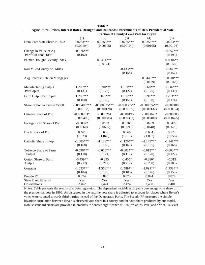
39

Table 2 Agricultural Prices, Interest Rates, Drought, and Railroads Determinants of 1896 Presidential Vote

Fraction of County-Level Vote for Bryan (1) (2) (3) (4) (5) Dem. Pres Vote Share in 1892 0.0253*** 0.0253*** 0.0255*** 0.0256*** 0.0253*** (0.00104) (0.00105) (0.00104) (0.00105) (0.00104) Change in Value of Ag -0.576*** -0.657*** Portfolio 1886-1895 (0.192) (0.193) Palmer Drought Severity Index 0.0414*** 0.0306** (0.0124) (0.0122) Rail Miles/County Sq. Miles -0.433*** -0.346** (0.158) (0.152) Avg. Interest Rate on Mortgages 0.0443*** 0.0518*** (0.0159) (0.0165) Manufacturing Output 1.208*** 1.090*** 1.101*** 1.068*** 1.146*** Per Capita (0.131) (0.126) (0.127) (0.125) (0.130) Farm Output Per Capita 1.280*** 1.167*** 1.136*** 1.091*** 1.263*** (0.160) (0.160) (0.151) (0.158) (0.174) Share of Pop in Cities>25000 -0.000405*** -0.000335*** -0.000305** -0.000374*** -0.000180 (0.000133) (0.000128) (0.000139) (0.000132) (0.000124) Chinese Share of Pop -0.000753* -0.000261 -0.000195 -0.0000402 -0.000303 (0.000405) (0.000385) (0.000382) (0.000400) (0.000425) Foreign Born Share of Pop -0.00322 0.0103 0.0766 0.0459 0.0429 (0.0660) (0.0655) (0.0695) (0.0648) (0.0678) Black Share of Pop 0.461 0.659 0.568 0.654 0.523 (1.023) (1.046) (1.019) (1.037) (1.056) Catholic Share of Pop -1.085*** -1.183*** -1.120*** -1.143*** -1.141*** (0.168) (0.168) (0.167) (0.165) (0.166) Tobacco Share of Farm -0.590*** -0.670*** -0.601*** -0.613*** -0.603*** Output (0.118) (0.121) (0.117) (0.120) (0.122) Cotton Share of Farm -0.459** -0.335 -0.405* -0.386* -0.313 Output (0.212) (0.212) (0.212) (0.208) (0.203) Constant -1.653*** -1.558*** -1.589*** -1.891*** -1.938*** (0.104) (0.105) (0.105) (0.146) (0.153) Pseudo R2 0.874 0.875 0.873 0.874 0.878 State Fixed Effects? Yes Yes Yes Yes Yes Observations 2,462 2,424 2,474 2,460 2,401 Notes: Table presents the results of a Beta regression. The dependent variable is Bryan’s percentage vote share of the presidential vote in 1896. As discussed in the text the vote share is adjusted to account for places where Bryan’s votes were counted towards third-parties instead of the Democratic Party. The Pseudo R2 measures the simple bivariate correlation between Bryan’s observed vote share in a county and the vote share predicted by our model. Robust standard errors are provided in brackets. * denotes significance at 10%; ** at 5% level and *** at 1% level.

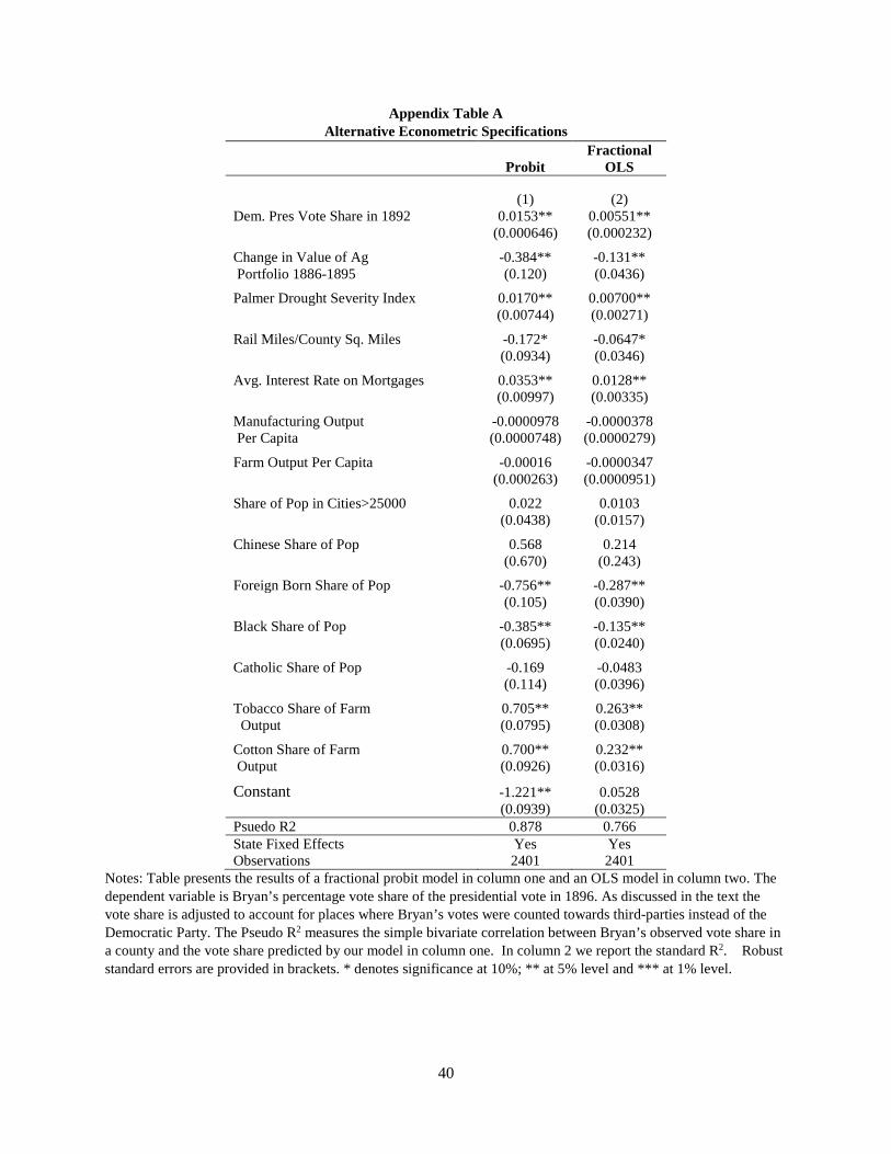
40

Appendix Table A Alternative Econometric Specifications

Probit Fractional

OLS

(1) (2) Dem. Pres Vote Share in 1892 0.0153** 0.00551** (0.000646) (0.000232) Change in Value of Ag -0.384** -0.131** Portfolio 1886-1895 (0.120) (0.0436) Palmer Drought Severity Index 0.0170** 0.00700** (0.00744) (0.00271) Rail Miles/County Sq. Miles -0.172* -0.0647* (0.0934) (0.0346) Avg. Interest Rate on Mortgages 0.0353** 0.0128** (0.00997) (0.00335) Manufacturing Output -0.0000978 -0.0000378 Per Capita (0.0000748) (0.0000279) Farm Output Per Capita -0.00016 -0.0000347 (0.000263) (0.0000951) Share of Pop in Cities>25000 0.022 0.0103 (0.0438) (0.0157) Chinese Share of Pop 0.568 0.214 (0.670) (0.243) Foreign Born Share of Pop -0.756** -0.287** (0.105) (0.0390) Black Share of Pop -0.385** -0.135** (0.0695) (0.0240) Catholic Share of Pop -0.169 -0.0483 (0.114) (0.0396) Tobacco Share of Farm 0.705** 0.263** Output (0.0795) (0.0308) Cotton Share of Farm 0.700** 0.232** Output (0.0926) (0.0316) Constant -1.221** 0.0528 (0.0939) (0.0325) Psuedo R2 0.878 0.766 State Fixed Effects Yes Yes Observations 2401 2401

Notes: Table presents the results of a fractional probit model in column one and an OLS model in column two. The dependent variable is Bryan’s percentage vote share of the presidential vote in 1896. As discussed in the text the vote share is adjusted to account for places where Bryan’s votes were counted towards third-parties instead of the Democratic Party. The Pseudo R2 measures the simple bivariate correlation between Bryan’s observed vote share in a county and the vote share predicted by our model in column one. In column 2 we report the standard R2. Robust standard errors are provided in brackets. * denotes significance at 10%; ** at 5% level and *** at 1% level.

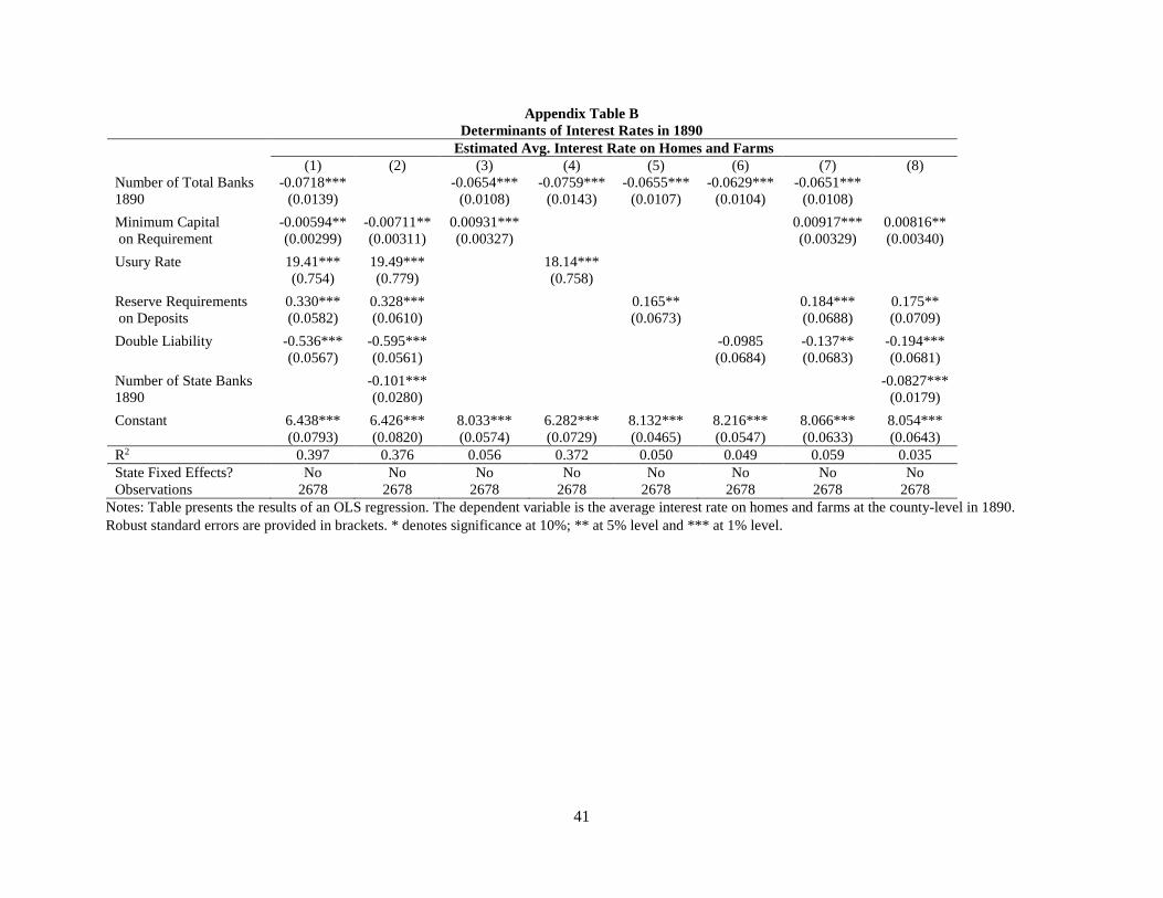
41

Appendix Table B Determinants of Interest Rates in 1890

Estimated Avg. Interest Rate on Homes and Farms (1) (2) (3) (4) (5) (6) (7) (8) Number of Total Banks -0.0718*** -0.0654*** -0.0759*** -0.0655*** -0.0629*** -0.0651*** 1890 (0.0139) (0.0108) (0.0143) (0.0107) (0.0104) (0.0108) Minimum Capital -0.00594** -0.00711** 0.00931*** 0.00917*** 0.00816** on Requirement (0.00299) (0.00311) (0.00327) (0.00329) (0.00340) Usury Rate 19.41*** 19.49*** 18.14*** (0.754) (0.779) (0.758) Reserve Requirements 0.330*** 0.328*** 0.165** 0.184*** 0.175** on Deposits (0.0582) (0.0610) (0.0673) (0.0688) (0.0709) Double Liability -0.536*** -0.595*** -0.0985 -0.137** -0.194*** (0.0567) (0.0561) (0.0684) (0.0683) (0.0681) Number of State Banks -0.101*** -0.0827*** 1890 (0.0280) (0.0179) Constant 6.438*** 6.426*** 8.033*** 6.282*** 8.132*** 8.216*** 8.066*** 8.054*** (0.0793) (0.0820) (0.0574) (0.0729) (0.0465) (0.0547) (0.0633) (0.0643) R2 0.397 0.376 0.056 0.372 0.050 0.049 0.059 0.035 State Fixed Effects? No No No No No No No No Observations 2678 2678 2678 2678 2678 2678 2678 2678

Notes: Table presents the results of an OLS regression. The dependent variable is the average interest rate on homes and farms at the county-level in 1890. Robust standard errors are provided in brackets. * denotes significance at 10%; ** at 5% level and *** at 1% level.

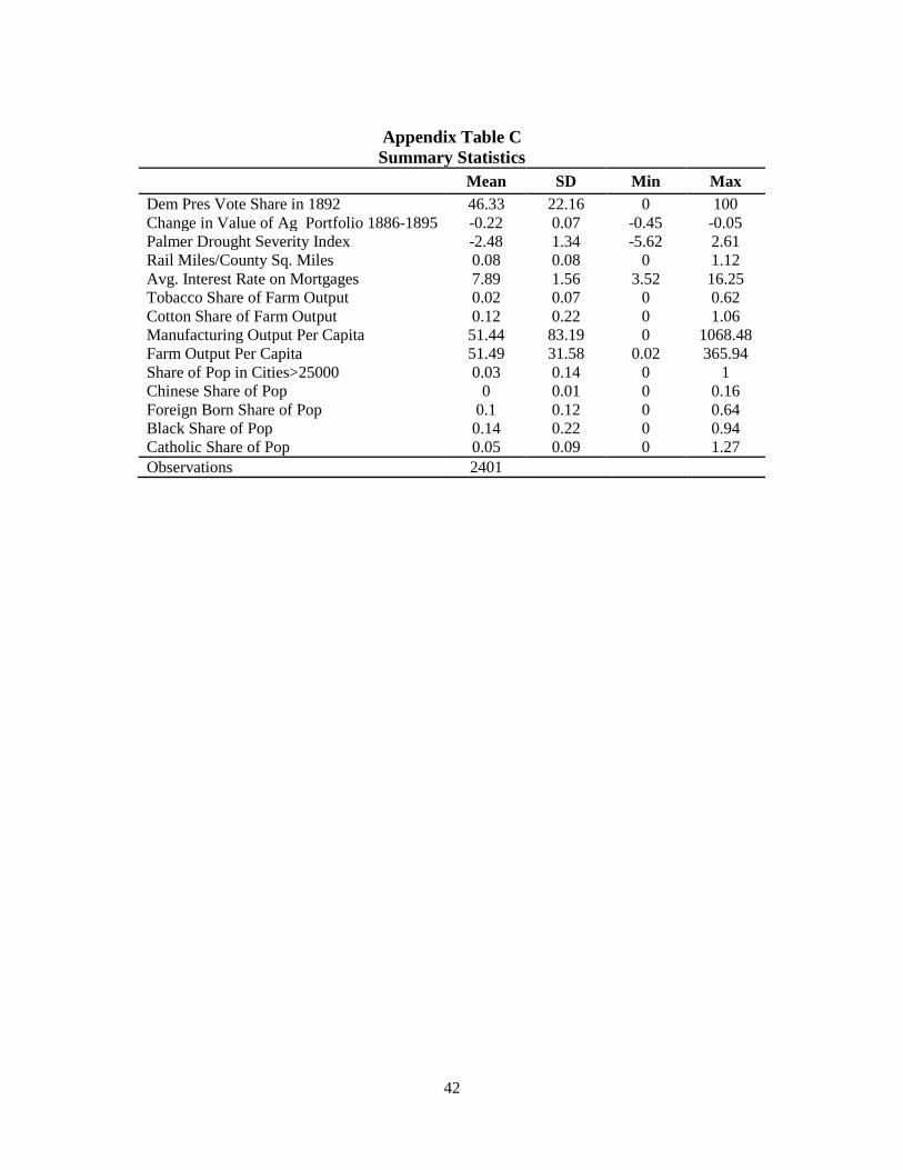
42

Appendix Table C Summary Statistics

Mean SD Min Max Dem Pres Vote Share in 1892 46.33 22.16 0 100 Change in Value of Ag Portfolio 1886-1895 -0.22 0.07 -0.45 -0.05 Palmer Drought Severity Index -2.48 1.34 -5.62 2.61 Rail Miles/County Sq. Miles 0.08 0.08 0 1.12 Avg. Interest Rate on Mortgages 7.89 1.56 3.52 16.25 Tobacco Share of Farm Output 0.02 0.07 0 0.62 Cotton Share of Farm Output 0.12 0.22 0 1.06 Manufacturing Output Per Capita 51.44 83.19 0 1068.48 Farm Output Per Capita 51.49 31.58 0.02 365.94 Share of Pop in Cities>25000 0.03 0.14 0 1 Chinese Share of Pop 0 0.01 0 0.16 Foreign Born Share of Pop 0.1 0.12 0 0.64 Black Share of Pop 0.14 0.22 0 0.94 Catholic Share of Pop 0.05 0.09 0 1.27 Observations 2401

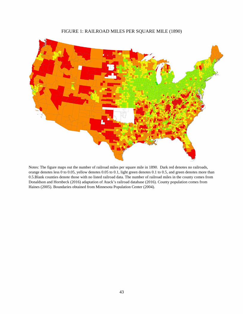
43

FIGURE 1: RAILROAD MILES PER SQUARE MILE (1890)

Notes: The figure maps out the number of railroad miles per square mile in 1890. Dark red denotes no railroads, orange denotes less 0 to 0.05, yellow denotes 0.05 to 0.1, light green denotes 0.1 to 0.5, and green denotes more than 0.5.Blank counties denote those with no listed railroad data. The number of railroad miles in the county comes from Donaldson and Hornbeck (2016) adaptation of Atack’s railroad database (2016). County population comes from Haines (2005). Boundaries obtained from Minnesota Population Center (2004).

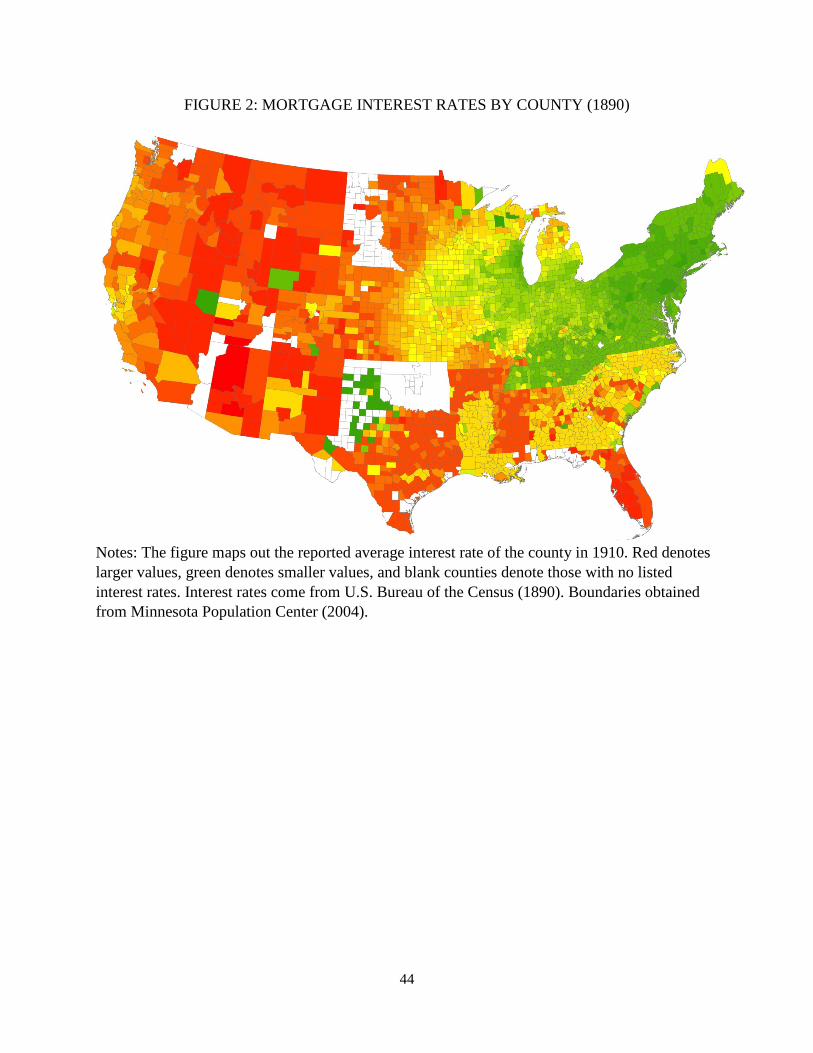
44

FIGURE 2: MORTGAGE INTEREST RATES BY COUNTY (1890)

Notes: The figure maps out the reported average interest rate of the county in 1910. Red denotes larger values, green denotes smaller values, and blank counties denote those with no listed interest rates. Interest rates come from U.S. Bureau of the Census (1890). Boundaries obtained from Minnesota Population Center (2004).

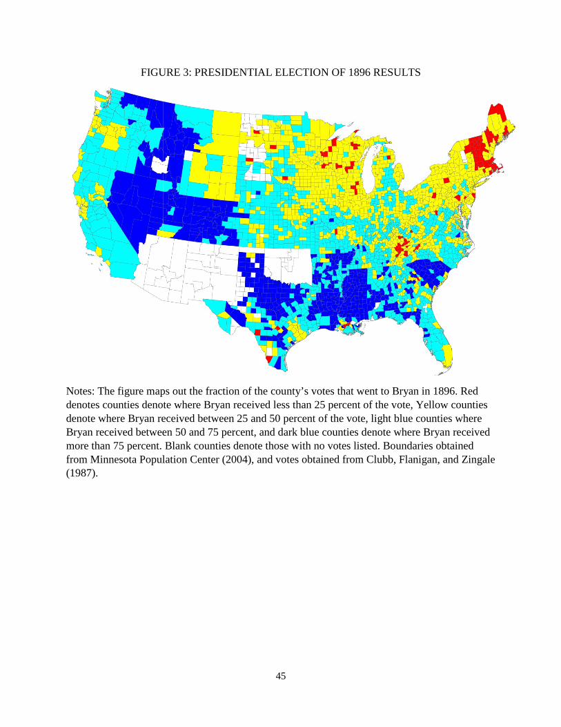
45

FIGURE 3: PRESIDENTIAL ELECTION OF 1896 RESULTS

Notes: The figure maps out the fraction of the county’s votes that went to Bryan in 1896. Red denotes counties denote where Bryan received less than 25 percent of the vote, Yellow counties denote where Bryan received between 25 and 50 percent of the vote, light blue counties where Bryan received between 50 and 75 percent, and dark blue counties denote where Bryan received more than 75 percent. Blank counties denote those with no votes listed. Boundaries obtained from Minnesota Population Center (2004), and votes obtained from Clubb, Flanigan, and Zingale (1987).

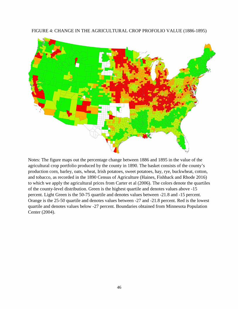
46

FIGURE 4: CHANGE IN THE AGRICULTURAL CROP PROFOLIO VALUE (1886-1895)

Notes: The figure maps out the percentage change between 1886 and 1895 in the value of the agricultural crop portfolio produced by the county in 1890. The basket consists of the county’s production corn, barley, oats, wheat, Irish potatoes, sweet potatoes, hay, rye, buckwheat, cotton, and tobacco, as recorded in the 1890 Census of Agriculture (Haines, Fishback and Rhode 2016) to which we apply the agricultural prices from Carter et al (2006). The colors denote the quartiles of the county-level distribution. Green is the highest quartile and denotes values above -15 percent. Light Green is the 50-75 quartile and denotes values between -21.8 and -15 percent. Orange is the 25-50 quartile and denotes values between -27 and -21.8 percent. Red is the lowest quartile and denotes values below -27 percent. Boundaries obtained from Minnesota Population Center (2004).

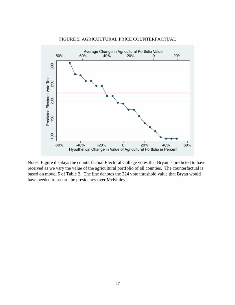
47

FIGURE 5: AGRICULTURAL PRICE COUNTERFACTUAL

Notes: Figure displays the counterfactual Electoral College votes that Bryan is predicted to have received as we vary the value of the agricultural portfolio of all counties. The counterfactual is based on model 5 of Table 2. The line denotes the 224 vote threshold value that Bryan would have needed to secure the presidency over McKinley.

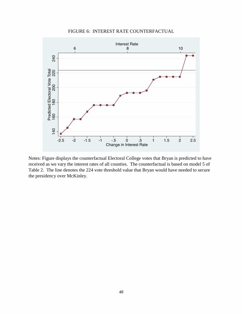
48

FIGURE 6: INTEREST RATE COUNTERFACTUAL

Notes: Figure displays the counterfactual Electoral College votes that Bryan is predicted to have received as we vary the interest rates of all counties. The counterfactual is based on model 5 of Table 2. The line denotes the 224 vote threshold value that Bryan would have needed to secure the presidency over McKinley.

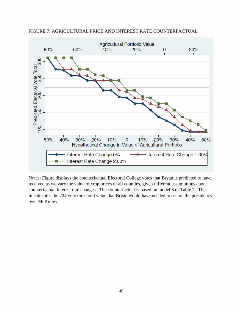
49

FIGURE 7: AGRICULTURAL PRICE AND INTEREST RATE COUNTERFACTUAL

Notes: Figure displays the counterfactual Electoral College votes that Bryan is predicted to have received as we vary the value of crop prices of all counties, given different assumptions about counterfactual interest rate changes. The counterfactual is based on model 5 of Table 2. The line denotes the 224 vote threshold value that Bryan would have needed to secure the presidency over McKinley.