pore pressure predict

DUG INSIGHT 3.1 USERMANUAL

Table of ContentsTable of ContentsPore Pressure Prediction .............................................................................................. 3

Module Summary .................................................................................................................................... 4

Well Settings ......................................................................................................................................... 14

Overburden Pressure (OBP)................................................................................................................. 18

Normal Compaction Trend Lines (NCTL)..............................................................................................21

Pore Pressure ....................................................................................................................................... 27

Calibration Points .................................................................................................................................. 35

Centroid Method — Pore Pressure in a Hydraulically-Connected Formation .......................................40

3D Model Building ................................................................................................................................. 43

View and Export Options....................................................................................................................... 57

Workflow Hints and FAQs ..................................................................................................................... 68

Pore Pressure Prediction

DUG Insight 3.1 User Manual

Module SummaryIntroduction

DUG Insight's Pore Pressure Prediction (PPP) module is a powerful tool for interactive geopressure analysis,calibration, and prediction at wells and in 3D.

More than 25% of drilling non-productive time (NPT) is due to overpressure. In addition to decreasing theNPT, correct prediction of the pressure regime enables faster drilling, less formation invasion, and thereforeimproved reservoir integrity.

Features include:

• Interactively model and predict overburden, pore, and fracture pressures.• 1D prediction and well calibration.• 3D prediction from seismic velocities.• Model centroid and fluid buoyancy effects including hydrocarbon column height.• Uncertainty simulation.• Eaton’s and Miller’s methods for pore pressure prediction.• Matthews-Kelly method for fracture gradient prediction.• Integrate calibration data (MDT, LOT, MW, etc).

The Pore Pressure Prediction module is a seamless addition to DUG Insight 3, with an intuitive, interactiveinterface for rapid analysis.

Operation modes and applications

The PPP module operates in two modes:

• 1D well calibration, and• 3D model building.

1D well calibration

1D well calibration allows the user to determine a local observed shale compaction trend line (OSCTL) andestablish a regional normal compaction trend line (NCTL) which best fits all well sonic and/or resistivity logs.

Overburden pressure (OBP) and thus pore pressure prediction (PPP) by either Eaton's or Miller's methods isdeveloped to best match measured or interpreted borehole pressures.

This module can be used for real time drilling and completion analyses, or as calibration points for 3D modelbuilding.

The calculated curves are also available to view in Insight's other 2D and 3D views.


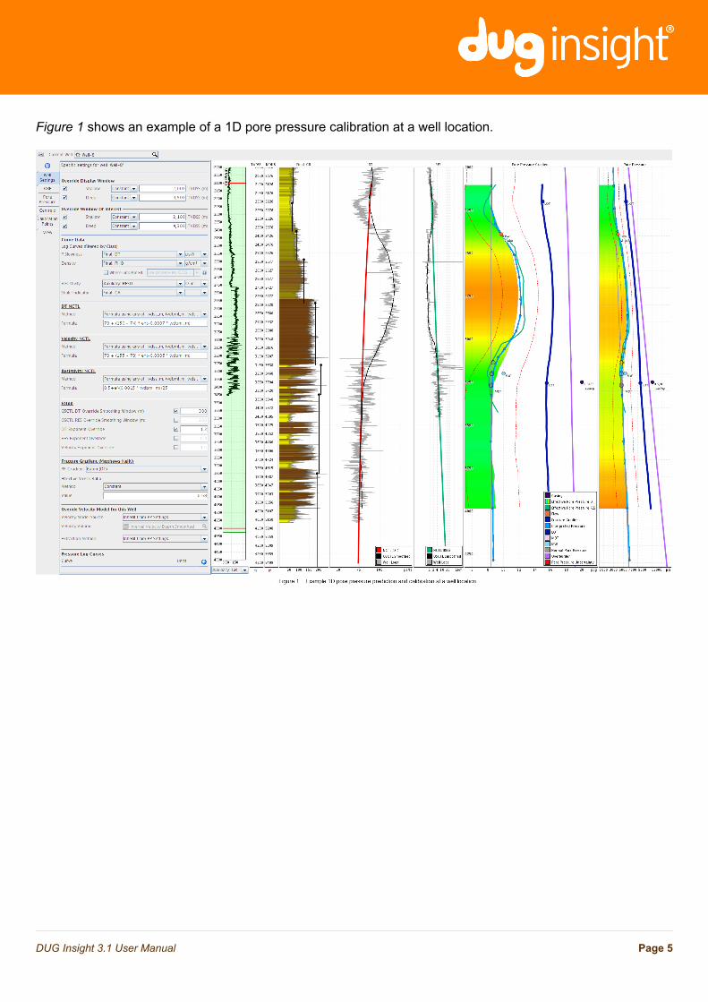
Figure 1 shows an example of a 1D pore pressure calibration at a well location.


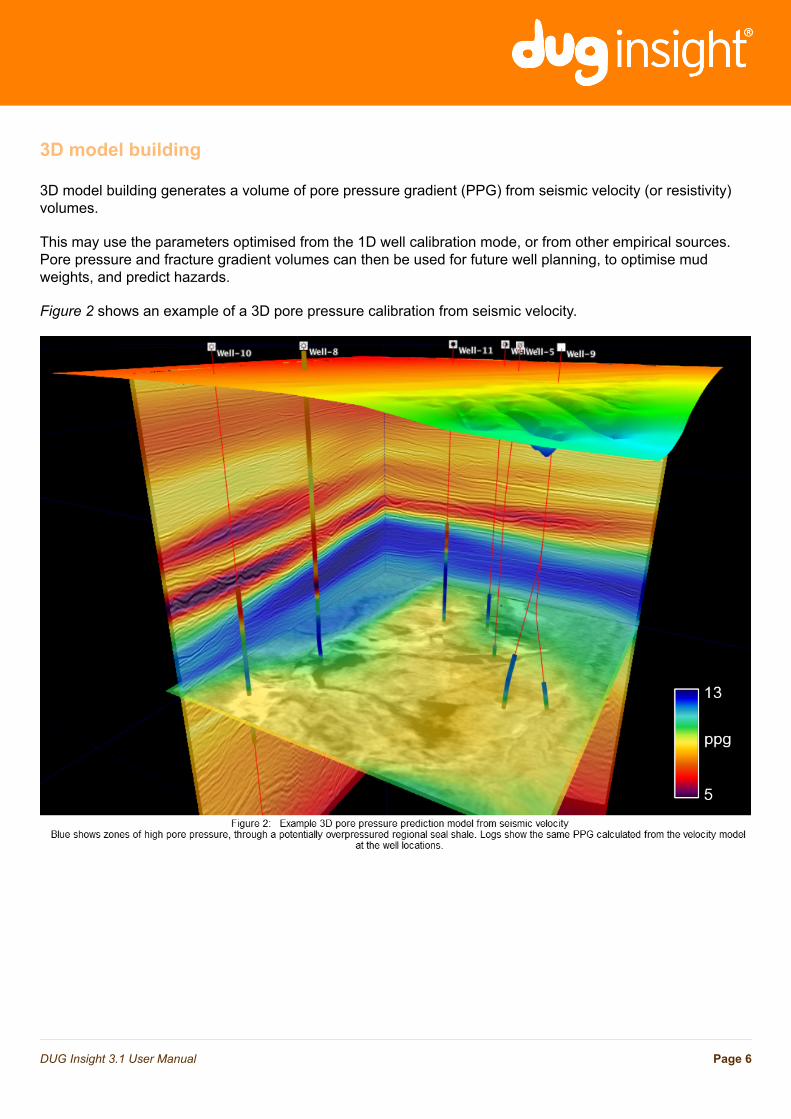
3D model building

3D model building generates a volume of pore pressure gradient (PPG) from seismic velocity (or resistivity)volumes.

This may use the parameters optimised from the 1D well calibration mode, or from other empirical sources.Pore pressure and fracture gradient volumes can then be used for future well planning, to optimise mudweights, and predict hazards.

Figure 2 shows an example of a 3D pore pressure calibration from seismic velocity.


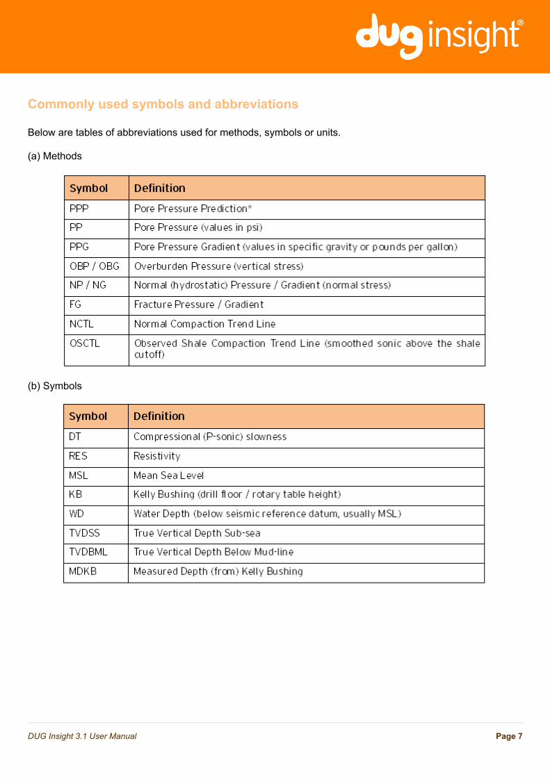
Commonly used symbols and abbreviations

Below are tables of abbreviations used for methods, symbols or units.

(a) Methods

(b) Symbols


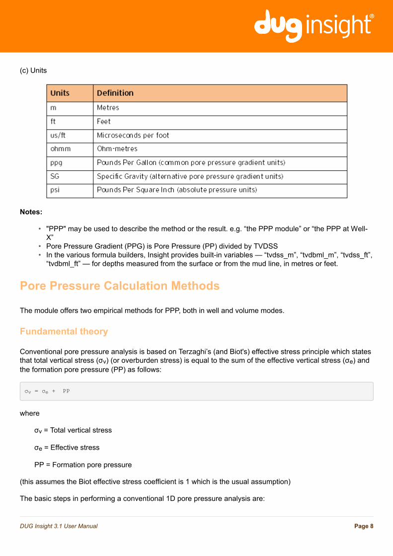
(c) Units

Notes:

• "PPP" may be used to describe the method or the result. e.g. “the PPP module” or “the PPP at Well-X”

• Pore Pressure Gradient (PPG) is Pore Pressure (PP) divided by TVDSS• In the various formula builders, Insight provides built-in variables — “tvdss_m”, “tvdbml_m”, “tvdss_ft”,

“tvdbml_ft” — for depths measured from the surface or from the mud line, in metres or feet.

Pore Pressure Calculation Methods

The module offers two empirical methods for PPP, both in well and volume modes.

Fundamental theory

Conventional pore pressure analysis is based on Terzaghi’s (and Biot's) effective stress principle which statesthat total vertical stress (σv) (or overburden stress) is equal to the sum of the effective vertical stress (σe) andthe formation pore pressure (PP) as follows:

σv = σe + PP

where

σv = Total vertical stress

σe = Effective stress

PP = Formation pore pressure

(this assumes the Biot effective stress coefficient is 1 which is the usual assumption)

The basic steps in performing a conventional 1D pore pressure analysis are:


1. Calculate total vertical stress (σv) from rock density.2. Estimate vertical effective stress (σe)from log measurements (DT or RES) or seismic (velocity).3. Pore pressure is then PP = σv - σe.4. Calibrate PP to credible information as it becomes available.

The pore pressure prediction module is utilised to estimate the effective stress (σe), using either Eaton's orMiller's methods, described next.

Eaton's equation

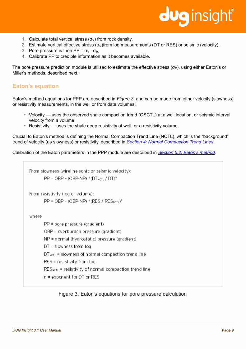
Eaton's method equations for PPP are described in Figure 3, and can be made from either velocity (slowness)or resistivity measurements, in the well or from data volumes:

• Velocity — uses the observed shale compaction trend (OSCTL) at a well location, or seismic intervalvelocity from a volume.

• Resistivity — uses the shale deep resistivity at well, or a resistivity volume.

Crucial to Eaton's method is defining the Normal Compaction Trend Line (NCTL), which is the “background”trend of velocity (as slowness) or resistivity, described in Section 4: Normal Compaction Trend Lines.

Calibration of the Eaton parameters in the PPP module are described in Section 5.2: Eaton's method.


Miller's equation

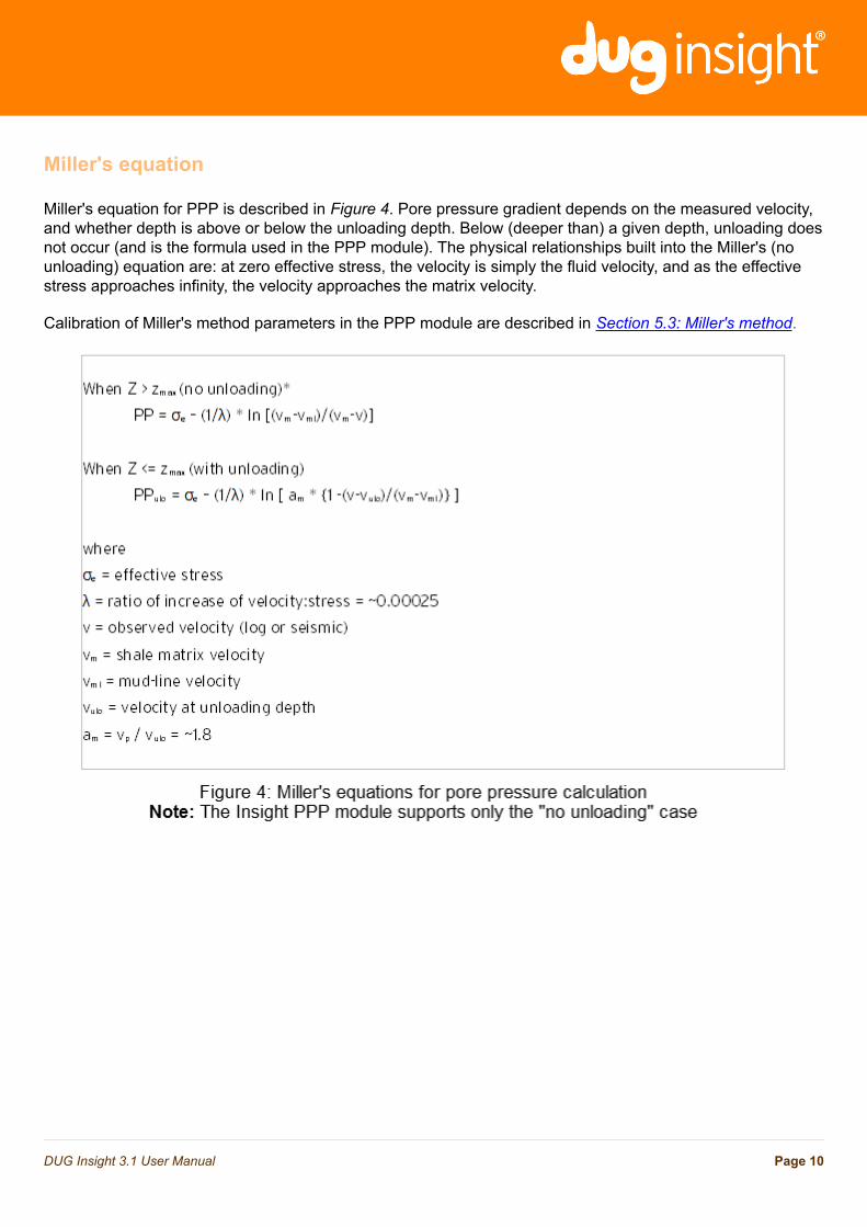
Miller's equation for PPP is described in Figure 4. Pore pressure gradient depends on the measured velocity,and whether depth is above or below the unloading depth. Below (deeper than) a given depth, unloading doesnot occur (and is the formula used in the PPP module). The physical relationships built into the Miller's (nounloading) equation are: at zero effective stress, the velocity is simply the fluid velocity, and as the effectivestress approaches infinity, the velocity approaches the matrix velocity.

Calibration of Miller's method parameters in the PPP module are described in Section 5.3: Miller's method.


Fracture gradient

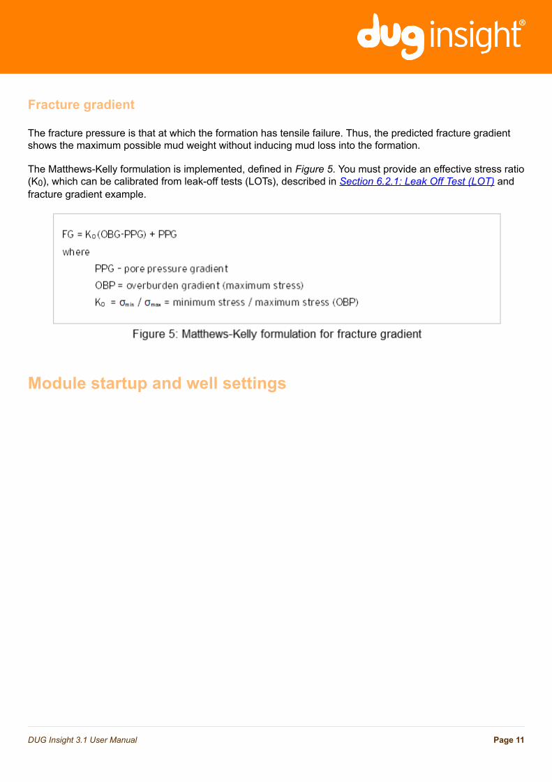
The fracture pressure is that at which the formation has tensile failure. Thus, the predicted fracture gradientshows the maximum possible mud weight without inducing mud loss into the formation.

The Matthews-Kelly formulation is implemented, defined in Figure 5. You must provide an effective stress ratio(K0), which can be calibrated from leak-off tests (LOTs), described in Section 6.2.1: Leak Off Test (LOT) andfracture gradient example.

Module startup and well settings


Starting the module

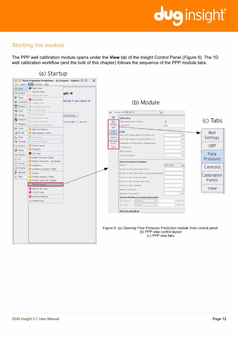
The PPP well calibration module opens under the View tab of the Insight Control Panel (Figure 6). The 1Dwell calibration workflow (and the bulk of this chapter) follows the sequence of the PPP module tabs.


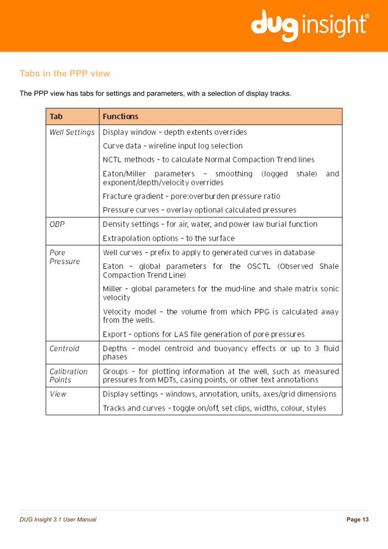
Tabs in the PPP view

The PPP view has tabs for settings and parameters, with a selection of display tracks.


Well Settings


Well data importing

The PPP module uses the same well data as the rest of DUG Insight. Importing well data into Insight iscovered in the Wells chapter.

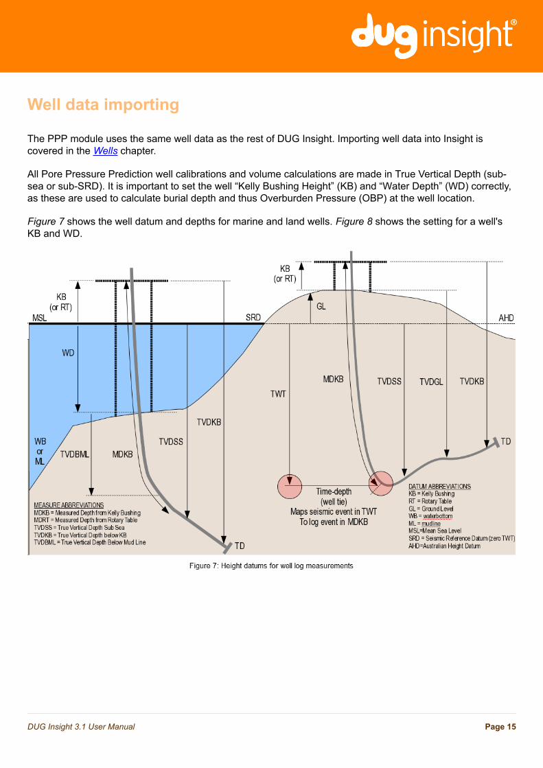
All Pore Pressure Prediction well calibrations and volume calculations are made in True Vertical Depth (sub-sea or sub-SRD). It is important to set the well “Kelly Bushing Height” (KB) and “Water Depth” (WD) correctly,as these are used to calculate burial depth and thus Overburden Pressure (OBP) at the well location.

Figure 7 shows the well datum and depths for marine and land wells. Figure 8 shows the setting for a well'sKB and WD.


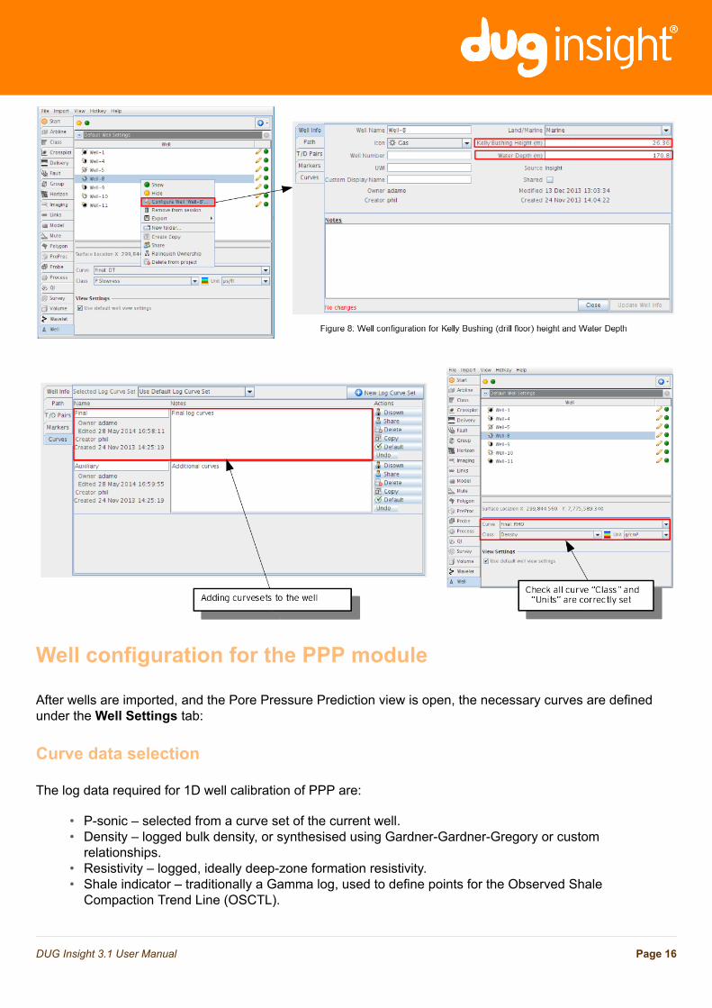
Well configuration for the PPP module

After wells are imported, and the Pore Pressure Prediction view is open, the necessary curves are definedunder the Well Settings tab:

Curve data selection

The log data required for 1D well calibration of PPP are:

• P-sonic – selected from a curve set of the current well.• Density – logged bulk density, or synthesised using Gardner-Gardner-Gregory or custom

relationships.• Resistivity – logged, ideally deep-zone formation resistivity.• Shale indicator – traditionally a Gamma log, used to define points for the Observed Shale

Compaction Trend Line (OSCTL).


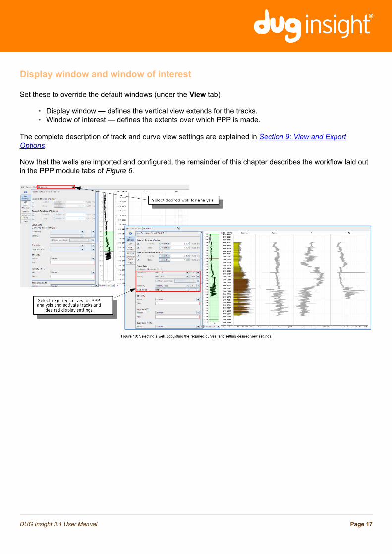
Display window and window of interest

Set these to override the default windows (under the View tab)

• Display window — defines the vertical view extends for the tracks.• Window of interest — defines the extents over which PPP is made.

The complete description of track and curve view settings are explained in Section 9: View and ExportOptions.

Now that the wells are imported and configured, the remainder of this chapter describes the workflow laid outin the PPP module tabs of Figure 6.


Overburden Pressure (OBP)Introduction

The overburden pressure (OBP) is the stress due to the weight of overlying rock. This is calculated thoughintegration of density, either via analytic extension of logs (1D well calibration mode) or a transform of velocityvolume (3D model building mode).

Parameter settings

Density options

The parameters to set and apply for all wells are:

• Air density — for log above sea level (if applicable)• Water density — for depths from sea level to the sea floor (default to 1.02 g/cc)• Default shallow power — power-law exponent to apply from the sea floor to the first log sample• Default deep power — exponent to use below the logged zone• Density volume (in TVD) — volume to use when Use density from volume is selected

Note: The water depth must be correct in the well configuration. To view or change the well configuration,open the Well tab in the Control Panel, and double-click the desired well (see Figure 8).

Extrapolation options

• Shallow zone — defines the zone from the sea floor to the (allocated) log depth.• Extrapolate up from — defines the first log depth from which to begin the density extrapolation up to

the sea floor. Zero (0) will use the first logged sample.• Override Power — if checked, will be applied for the current well only.• Deep zone — defines the zone from the last log depth to the base of Display Window.• Extrapolate down — either from a user-defined depth, from the last log sample, or do not

extrapolate.• Method — either power-law or polynomial GGG relationship.


Volume options

To calculate PPP volumes, an OBP volume is also required. Section 8: 3D Model Building shows how tocreate a density volume, which is used to calculate the OBP volume.

QC measures


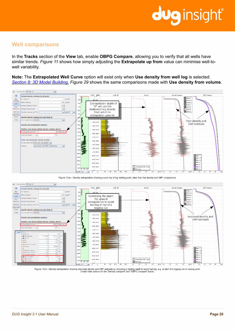
Well comparisons

In the Tracks section of the View tab, enable OBPG Compare, allowing you to verify that all wells havesimilar trends. Figure 11 shows how simply adjusting the Extrapolate up from value can minimise well-to-well variability.

Note: The Extrapolated Well Curve option will exist only when Use density from well log is selected.Section 8: 3D Model Building, Figure 29 shows the same comparisons made with Use density from volume.


Normal Compaction Trend Lines (NCTL)Introduction

The Normal Compaction Trend Line (NCTL) represents the sonic and resistivity values if the pore pressurewere normal (hydrostatic). There are three potential NCTLs to consider:

• DT NCTL — a model for the current well's (smoothed) P-sonic log, or• Resistivity NCTL — a model for the current well's (smoothed) resistivity log, or• Velocity NCTL — the compaction trend for making PPP from seismic interval velocity (see Section 8:

3D Model Building).

Note: The smoothed DT and Resistivity are defined as the “Observed Shale Compaction Trend Line(OSCTL)” (see Section 5.2.1: Observed Shale Compaction Trend Line (OSCTL) for an overview of theOSCTL generation from logs).


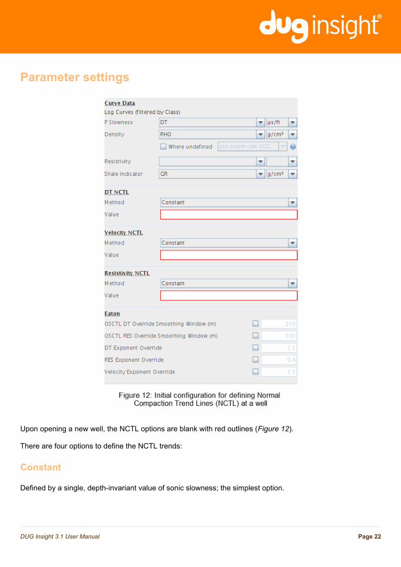
Parameter settings

Upon opening a new well, the NCTL options are blank with red outlines (Figure 12).

There are four options to define the NCTL trends:

Constant

Defined by a single, depth-invariant value of sonic slowness; the simplest option.


Log

NCTL defined from a log curve.

Picked

Manually picking a curve on the DT or Resistivity tracks:

1. Under the Method drop-down, select Picked.2. To begin picking on the relevant track (DT or RES), right click and choose Start Picking NCTL.3. Left click to add NCTL picks at any depth and position; NCTL is linearly interpolated between picks.4. Left click and drag on the line to move the entire line.5. Left click and drag on a pick to move one pick; right click to delete a pick.6. Right click and choose Stop Picking NCTL.

Formula

These are depth-dependent functions of “tvdss_m”, “tvdbml_m”, “tvdss_ft”, “tvdbml_ft”, where the suffix “_ss”indicates sub-sea, and “_bml” is below mud-line (or burial depth).

The default NCTL formulae are of the form:

For P-slowness (DT)

NCTL = DT + (DTm - DT) * e^c*tvdbml_m

where default settings are

DT = 50 us/ft (reference sonic slowness)

DTm = 185 us/ft (mud-line sonic slowness)

c = -0.0006

that is

NCTL = 50 + (185 - 50) * e^(-0.0006 * tvdbml_m)

For resistivity (RES)

NCTL = tvdss_m / k

with default setting

k= 5000


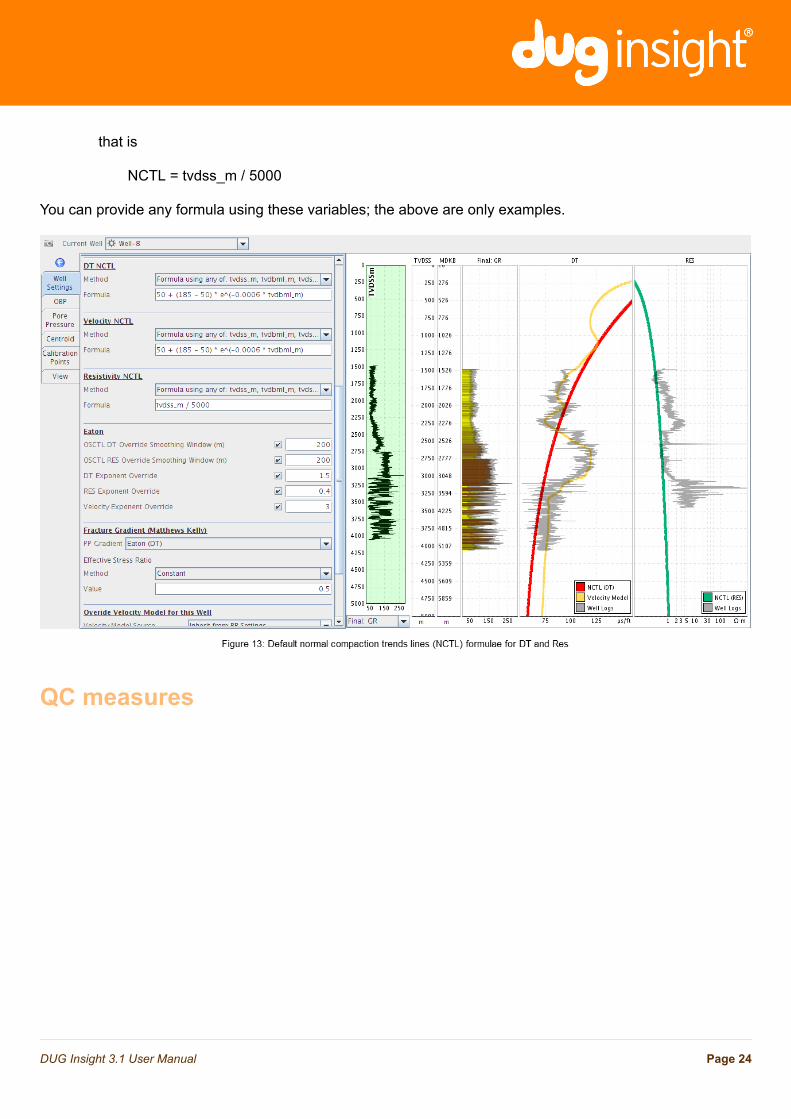
that is

NCTL = tvdss_m / 5000

You can provide any formula using these variables; the above are only examples.

QC measures


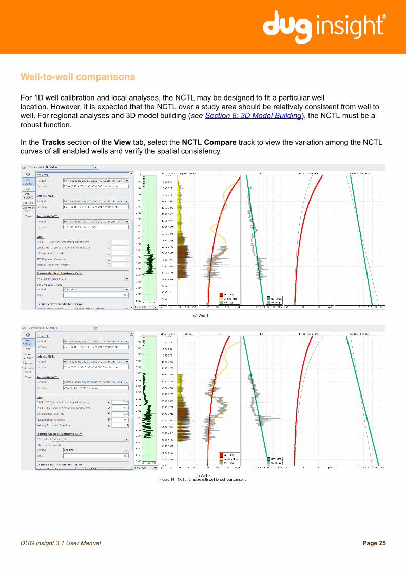
Well-to-well comparisons

For 1D well calibration and local analyses, the NCTL may be designed to fit a particular welllocation. However, it is expected that the NCTL over a study area should be relatively consistent from well towell. For regional analyses and 3D model building (see Section 8: 3D Model Building), the NCTL must be arobust function.

In the Tracks section of the View tab, select the NCTL Compare track to view the variation among the NCTLcurves of all enabled wells and verify the spatial consistency.


Pressure comparisons

The NCTL may be iteratively adjusted such that pore pressure predictions match measured or interpretedpressures. Thus, the NCTL may be revisited and updated once pore pressure predictions are made from thelogs (see Section 5.2: Eaton's method) or volumes (see Section 8.3: 3D volume generation).


Pore PressureIntroduction

The complete set of default parameters for well pressure predictions, visualisation, and exporting arecontrolled from this tab: Eaton and Miller parameters, velocity model, and LAS exports.

Eaton's method

Eaton's method predicts pore pressure from either velocity or resistivity, using equations shown in Figure 3(Section 1.3.2: Eaton's equation). These both require a normal compaction trend line (NCTL) and overburdenpressure (OBP), which may be well-local or regional models.


Observed Shale Compaction Trend Line (OSCTL)

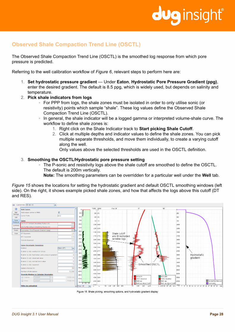
The Observed Shale Compaction Trend Line (OSCTL) is the smoothed log response from which porepressure is predicted.

Referring to the well calibration workflow of Figure 6, relevant steps to perform here are:

1. Set hydrostatic pressure gradient — Under Eaton, Hydrostatic Pore Pressure Gradient (ppg),enter the desired gradient. The default is 8.5 ppg, which is widely used, but depends on salinity andtemperature.

2. Pick shale indicators from logs◦ For PPP from logs, the shale zones must be isolated in order to only utilise sonic (or

resistivity) points which sample “shale”. These log values define the Observed ShaleCompaction Trend Line (OSCTL).

◦ In general, the shale indicator will be a logged gamma or interpreted volume-shale curve. Theworkflow to define shale zones is:

1. Right click on the Shale Indicator track to Start picking Shale Cutoff.2. Click at multiple depths and indicator values to define the shale zones. You can pick

multiple separate thresholds, and move them individually, to create a varying cutoffalong the well.Only values above the selected thresholds are used in the OSCTL definition.

3. Smoothing the OSCTL/Hydrostatic pore pressure setting◦ The P-sonic and resistivity logs above the shale cutoff are smoothed to define the OSCTL.

The default is 200m vertically.Note: The smoothing parameters can be overridden for a particular well under the Well tab.

Figure 15 shows the locations for setting the hydrostatic gradient and default OSCTL smoothing windows (leftside). On the right, it shows example picked shale zones, and how that affects the logs above this cutoff (DTand RES).


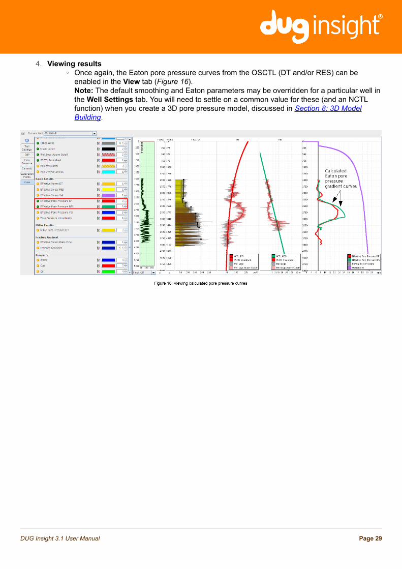
4. Viewing results◦ Once again, the Eaton pore pressure curves from the OSCTL (DT and/or RES) can be

enabled in the View tab (Figure 16).Note: The default smoothing and Eaton parameters may be overridden for a particular well inthe Well Settings tab. You will need to settle on a common value for these (and an NCTLfunction) when you create a 3D pore pressure model, discussed in Section 8: 3D ModelBuilding.


Velocity model and interpreted pressure curves

There are two other options for pore pressure prediction at a well location:

• Velocity model — If a seismic velocity volume is available, this may be used for predictions awayfrom the borehole, and/or ahead of the drill bit (where no wireline data is logged). This will use globalNCTL and OBP models. The relevant 1D well location calibration / 3D model building workflow andQCs are outlined in more detail in Section 8: 3D Model Building.

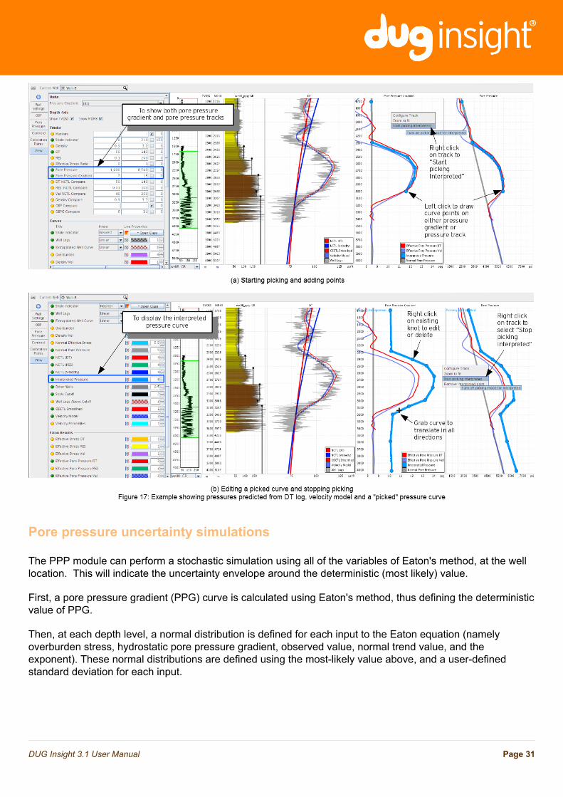
• Interpreted pressure — A pore pressure curve may be “picked” at a well location, based on thepredicted pressures (from either the Eaton or Miller methods) and/or other calibration points (seeSection 6: Calibration Points for more detail). To manually interpret a pressure curve, on either thepore pressure gradient or pore pressure tracks, right-click to choose Start picking Interpreted. Left-click to add a point, right-click to remove a point, or left-click and hold to drag the picked curve.

Figure 17 shows an example of a manually-picked curve.


Pore pressure uncertainty simulations

The PPP module can perform a stochastic simulation using all of the variables of Eaton's method, at the welllocation. This will indicate the uncertainty envelope around the deterministic (most likely) value.

First, a pore pressure gradient (PPG) curve is calculated using Eaton's method, thus defining the deterministicvalue of PPG.

Then, at each depth level, a normal distribution is defined for each input to the Eaton equation (namelyoverburden stress, hydrostatic pore pressure gradient, observed value, normal trend value, and theexponent). These normal distributions are defined using the most-likely value above, and a user-definedstandard deviation for each input.


We then randomly sample (using Monte Carlo simulation) from the distributions to create realisations of PPGat each depth level. The P10 and P90 curves are then calculated from this resulting distribution (which may ormay not be a normal distribution).

Under the Pore Pressure tab, Eaton Uncertainty Simulation section, relative uncertainties can be set for allEaton parameters (equations shown in Figure 3).

The specified “Number of random simulations” are then made at the given ”Sample Interval”.

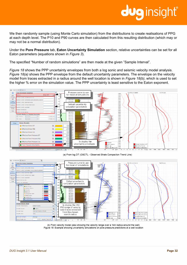
Figure 18 shows the PPP uncertainty envelopes from both a log sonic and seismic velocity model analysis.Figure 18(a) shows the PPP envelope from the default uncertainty parameters. The envelope on the velocitymodel from traces extracted in a radius around the well location is shown in Figure 18(b), which is used to setthe higher % error on the simulation value. The PPP uncertainty is least sensitive to the Eaton exponent.


Miller's method

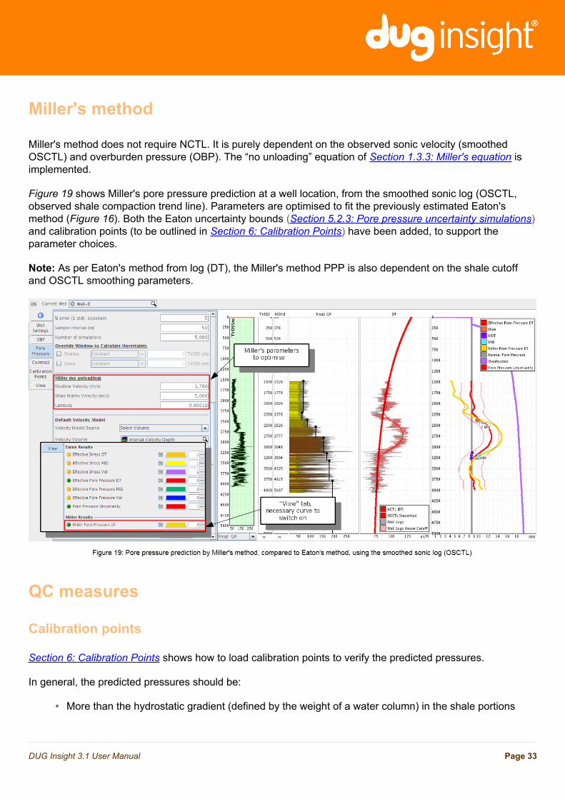
Miller's method does not require NCTL. It is purely dependent on the observed sonic velocity (smoothedOSCTL) and overburden pressure (OBP). The “no unloading” equation of Section 1.3.3: Miller's equation isimplemented.

Figure 19 shows Miller's pore pressure prediction at a well location, from the smoothed sonic log (OSCTL,observed shale compaction trend line). Parameters are optimised to fit the previously estimated Eaton'smethod (Figure 16). Both the Eaton uncertainty bounds (Section 5.2.3: Pore pressure uncertainty simulations)and calibration points (to be outlined in Section 6: Calibration Points) have been added, to support theparameter choices.

Note: As per Eaton's method from log (DT), the Miller's method PPP is also dependent on the shale cutoffand OSCTL smoothing parameters.

QC measures

Calibration points

Section 6: Calibration Points shows how to load calibration points to verify the predicted pressures.

In general, the predicted pressures should be:

• More than the hydrostatic gradient (defined by the weight of a water column) in the shale portions


• Less than the mud weight (if well is drilled “overbalanced”)• Less than the fracture gradient (which is calibrated to Leak Off Tests, unless the formation is already

fractured).

Uncertainty bounds and other data sources and methods

Pressures predicted by the two methods (Eaton's via sonic velocity, log resistivity, and seismic velocity; andMiller's from sonic log) would be expected to agree within the measurement and parameter uncertainties(which can be simulated for Eaton's method).


Calibration PointsIntroduction

The pore pressure track can be annotated with relevant borehole data, such as MDT (modular dynamic test),LOT (leak off tests), mud weights, flow tests, and casing points.

Manually adding points

When there are only a few points, manual entry may be the simplest route.


Leak Off Test (LOT) and fracture gradient example

Leak Off Test points are a useful guide to calibrate the fracture gradient.

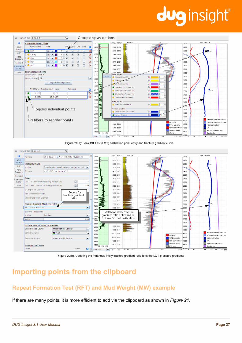
In the Calibration points tab, Calibration Point Groups section, create a new group called “LOT”. Selectthe units in which you will enter points: either psi (pressure) or ppg/SG (pressure gradient).

To add a row, click the Add icon (+) under Edit Calibration Points. Type the depth, pressure (or pressuregradient), and a label/comment as desired.

These points may be reordered by dragging the handle on the left side of the row. Display options for eachgroup (point colour, size) are alongside the “Group Name”. Figure 20(a) shows the completed LOT entriesand their positions on the PPG track.

The LOT can be used to calibrate the fracture gradient. The Matthews/Kelly fracture gradient is the ratiobetween the OBP (overburden pressure) and the PPP (pore pressure prediction), and is set under the WellSettings tab.

First, choose a source for the pore pressure: the Eaton calculation, a log curve, or an interpreted curve. Themethods for the OBP-PPG ratio are similar to the PPP methods described in Section 5. Pore Pressure -typically a “Constant” ratio is chosen. The “Value” (which defaults to 0.5) can then be updated to best fit theLOT calibration points, as shown in Figure 20(b).

Note: Deleting a Calibration Point Group will remove ALL points from ALL wells.


Importing points from the clipboard

Repeat Formation Test (RFT) and Mud Weight (MW) example

If there are many points, it is more efficient to add via the clipboard as shown in Figure 21.


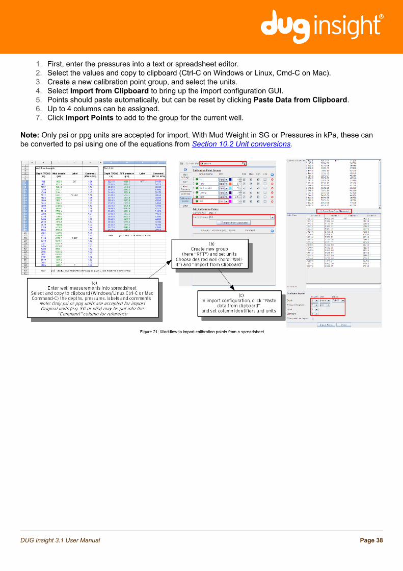
1. First, enter the pressures into a text or spreadsheet editor.2. Select the values and copy to clipboard (Ctrl-C on Windows or Linux, Cmd-C on Mac).3. Create a new calibration point group, and select the units.4. Select Import from Clipboard to bring up the import configuration GUI.5. Points should paste automatically, but can be reset by clicking Paste Data from Clipboard.6. Up to 4 columns can be assigned.7. Click Import Points to add to the group for the current well.

Note: Only psi or ppg units are accepted for import. With Mud Weight in SG or Pressures in kPa, these canbe converted to psi using one of the equations from Section 10.2 Unit conversions.


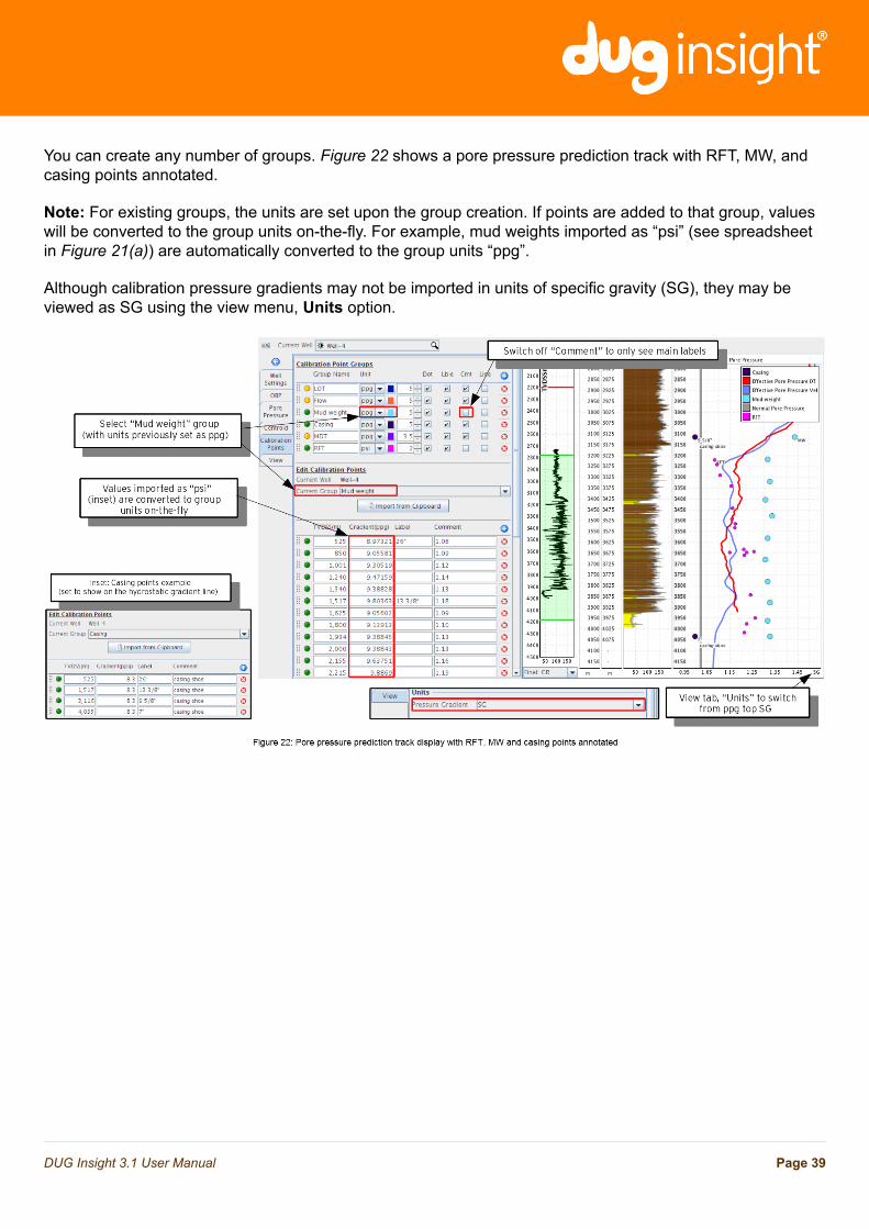
You can create any number of groups. Figure 22 shows a pore pressure prediction track with RFT, MW, andcasing points annotated.

Note: For existing groups, the units are set upon the group creation. If points are added to that group, valueswill be converted to the group units on-the-fly. For example, mud weights imported as “psi” (see spreadsheetin Figure 21(a)) are automatically converted to the group units “ppg”.

Although calibration pressure gradients may not be imported in units of specific gravity (SG), they may beviewed as SG using the view menu, Units option.


Centroid Method — Pore Pressure in aHydraulically-Connected FormationIntroduction

The concept of the centroid was described by Traugott (1997), and has also been referred to as “lateralpressure transfer” (Yardley and Swarbrick, 2001). The concept assumes that there is a midpoint or centre-point (the centroid) along a dipping sequence of permeable reservoirs and sealing non-reservoirs where thepore pressure in both is the same (pressure equilibrium). At this point, the predicted pore pressure (in thesealing non-reservoir) is assumed to be equal to the measured pore pressure in the porous reservoir.

In a hydraulically-connected formation, deeper overpressured areas are connected to shallower areas by apermeable layer. As a result, fluid flow along such a pathway can cause pressures to increase at the crest ofstructure – a common drilling target.

The relationship between predicted and measured pore pressure can be complicated, and an understandingof the relevant geological factors involved (compaction disequilibrium, seal breach, geologic and structuralsetting, etc.) is important. The measured pore pressure in the reservoir will usually follow the hydrostaticgradient of the formation fluid. The pressure in a hydraulically-connected formation can be calculated basedon the difference in the heights of the fluid columns.

The centroid method can be used to predict the pore pressure in a porous reservoir (or hydraulically-connected formation) using formation fluid density and fluid column height, and can be calibrated to measuredformation pressures in the well bore.


Creating and viewing

In the Centroid tab, add one or more fluids. Then in the View tab, toggle on each of the respective fluids todisplay. Figure 23(a) shows this initial setup.

QC measures


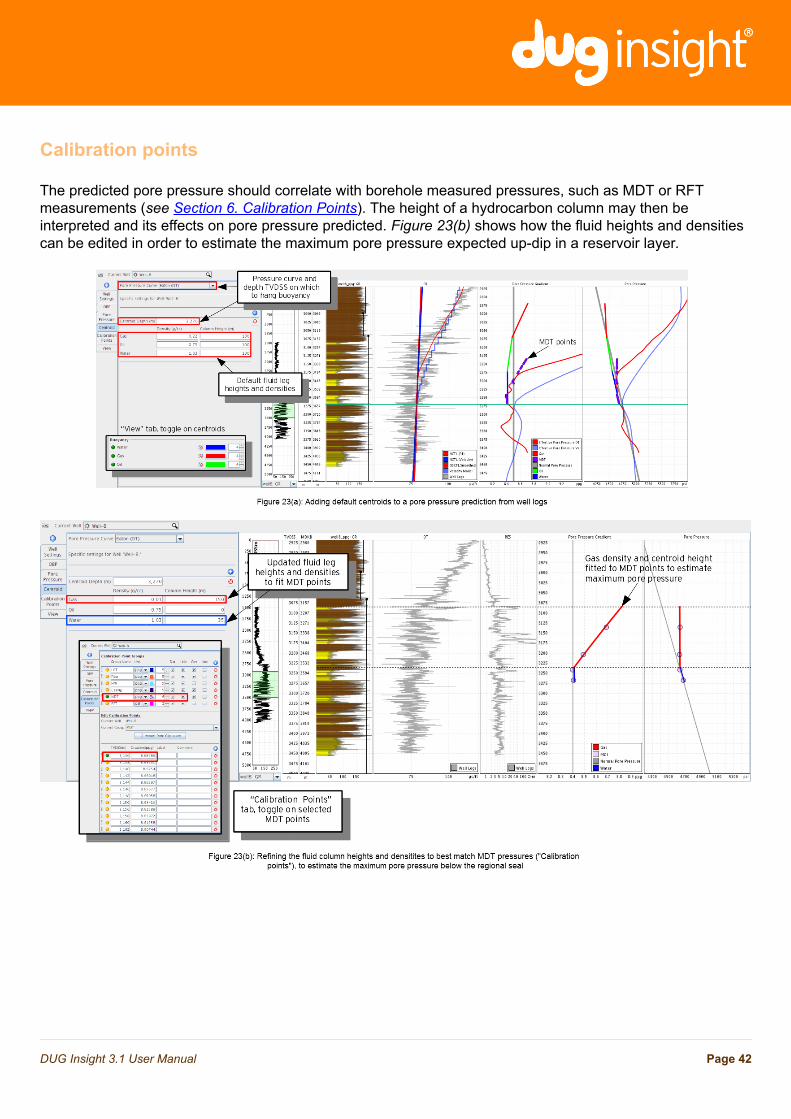
Calibration points

The predicted pore pressure should correlate with borehole measured pressures, such as MDT or RFTmeasurements (see Section 6. Calibration Points). The height of a hydrocarbon column may then beinterpreted and its effects on pore pressure predicted. Figure 23(b) shows how the fluid heights and densitiescan be edited in order to estimate the maximum pore pressure expected up-dip in a reservoir layer.


3D Model Building


Introduction

The second mode of the PPP module is 3D model building. This will use the calibration parameters (i.e.overburden pressures, NCTL models, and Eaton exponents) plus a 3D velocity model.

The 3D model building processes are found in the main Control Panel Process tab. As with other processes,these create new output volumes for use throughout Insight, including within the PPP view.

However, before building a 3D model of PPP from the velocity model, it should be verified at the wells. Thesame 1D well calibration workflow from Section 4: Normal Compaction Trend Lines (NCTL) and Section 5:Pore Pressure apply, but instead will use a global NCTL volume (for Eaton's method) and OBP volume, withthe aim of creating a 3D model that will tie the wells.

Volume preparation and 1D well verification

Velocity volume preparation

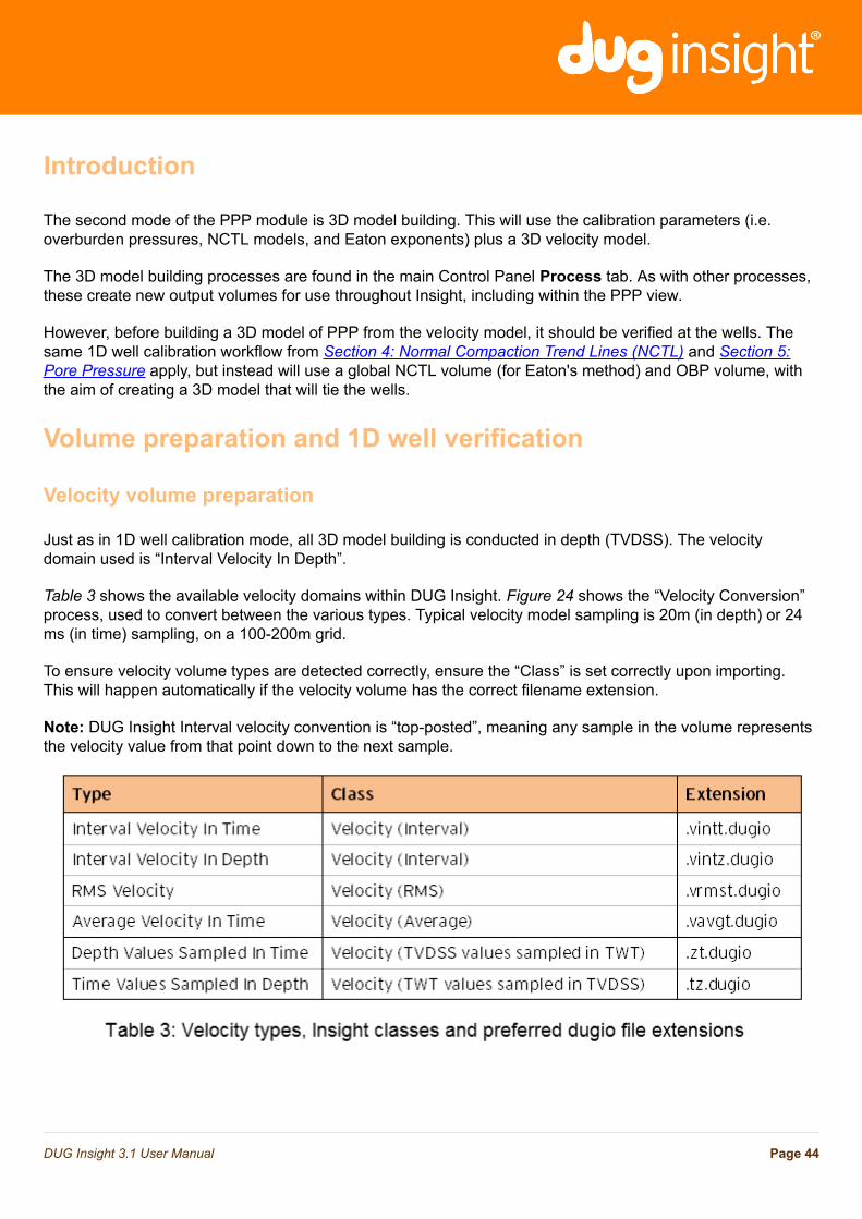
Just as in 1D well calibration mode, all 3D model building is conducted in depth (TVDSS). The velocitydomain used is “Interval Velocity In Depth”.

Table 3 shows the available velocity domains within DUG Insight. Figure 24 shows the “Velocity Conversion”process, used to convert between the various types. Typical velocity model sampling is 20m (in depth) or 24ms (in time) sampling, on a 100-200m grid.

To ensure velocity volume types are detected correctly, ensure the “Class” is set correctly upon importing.This will happen automatically if the velocity volume has the correct filename extension.

Note: DUG Insight Interval velocity convention is “top-posted”, meaning any sample in the volume representsthe velocity value from that point down to the next sample.


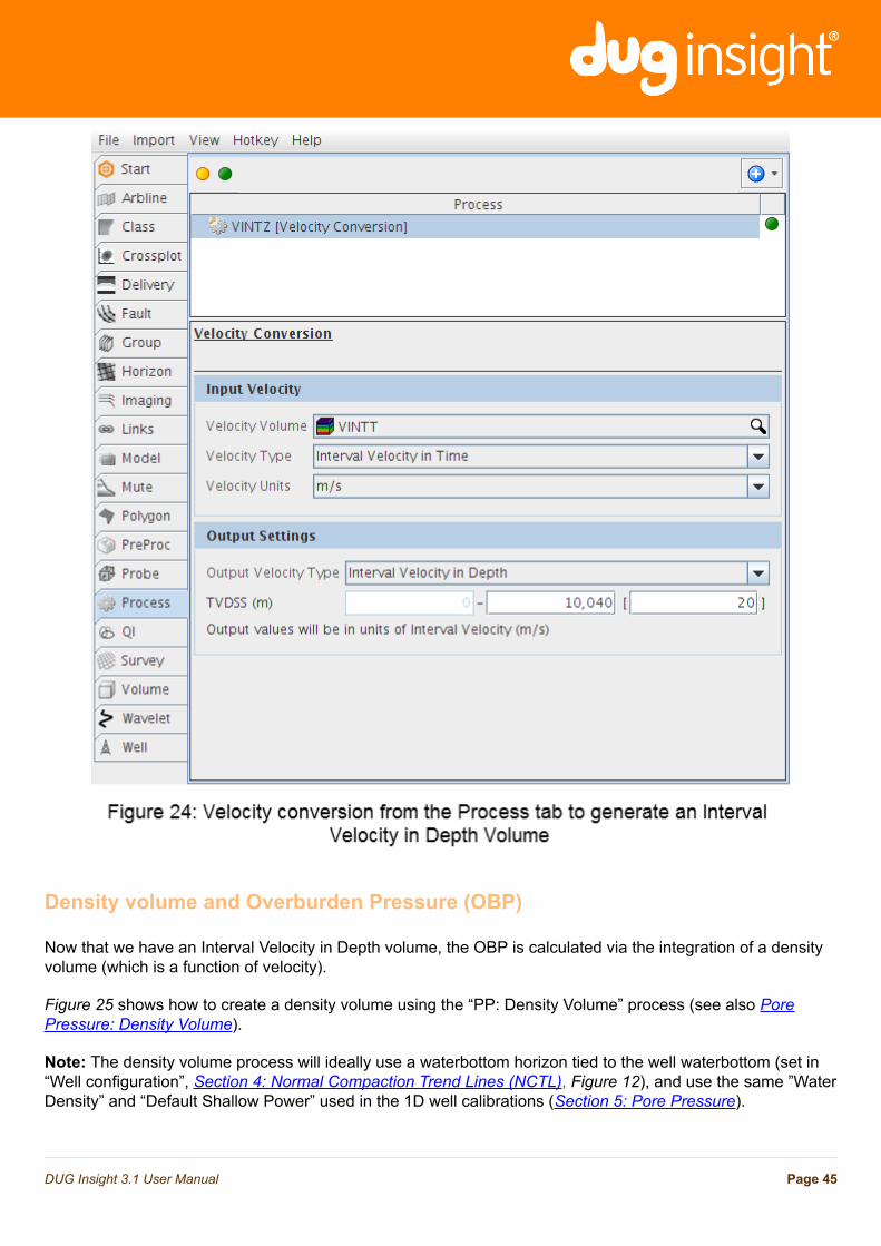
Density volume and Overburden Pressure (OBP)

Now that we have an Interval Velocity in Depth volume, the OBP is calculated via the integration of a densityvolume (which is a function of velocity).

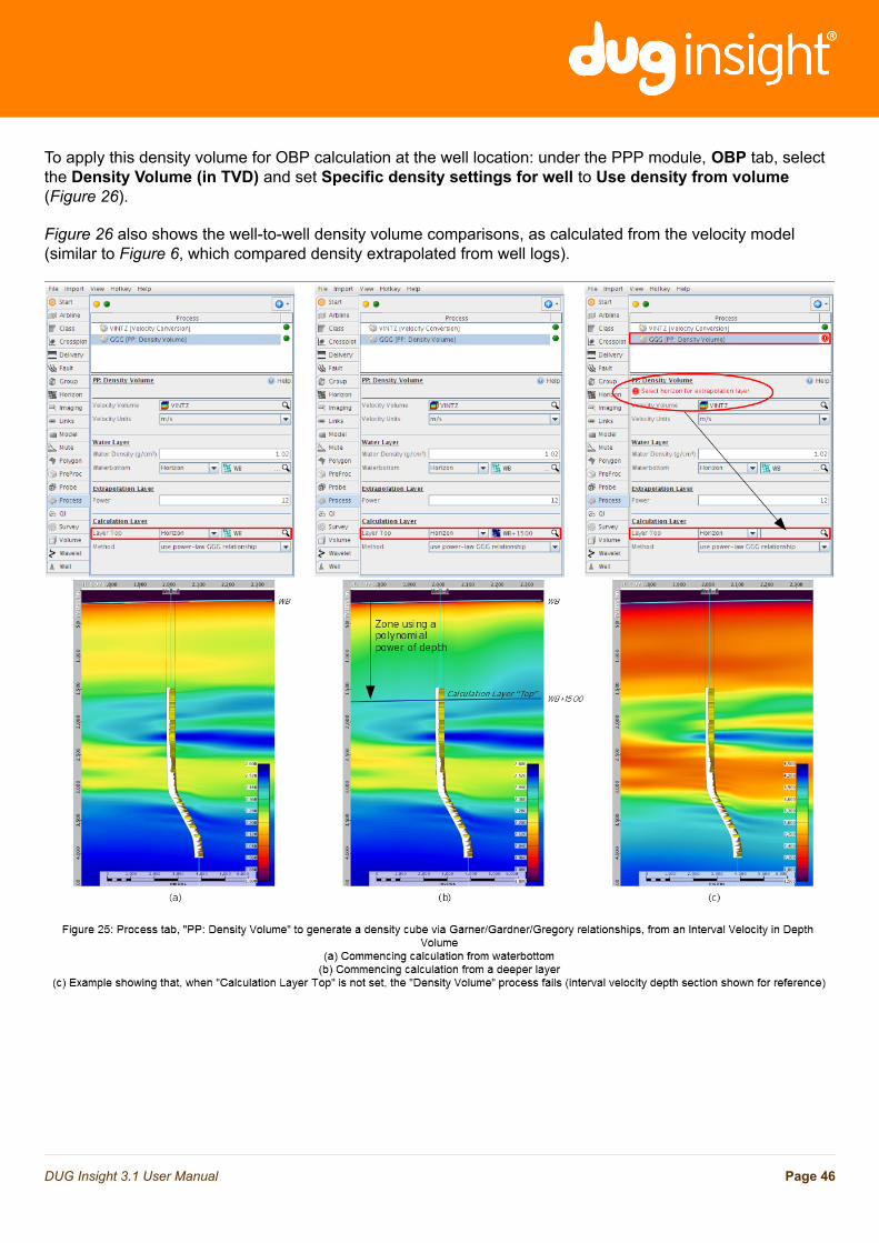
Figure 25 shows how to create a density volume using the “PP: Density Volume” process (see also PorePressure: Density Volume).

Note: The density volume process will ideally use a waterbottom horizon tied to the well waterbottom (set in“Well configuration”, Section 4: Normal Compaction Trend Lines (NCTL), Figure 12), and use the same ”WaterDensity” and “Default Shallow Power” used in the 1D well calibrations (Section 5: Pore Pressure).


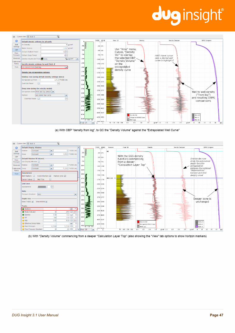
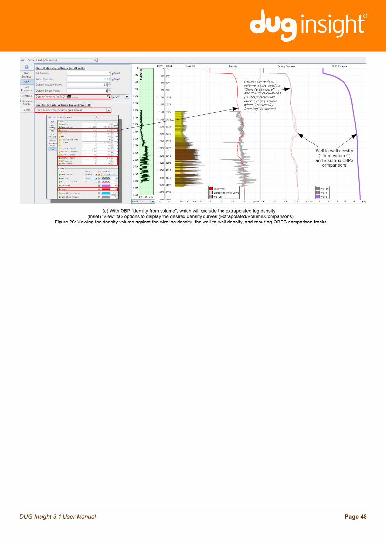
To apply this density volume for OBP calculation at the well location: under the PPP module, OBP tab, selectthe Density Volume (in TVD) and set Specific density settings for well to Use density from volume(Figure 26).

Figure 26 also shows the well-to-well density volume comparisons, as calculated from the velocity model(similar to Figure 6, which compared density extrapolated from well logs).


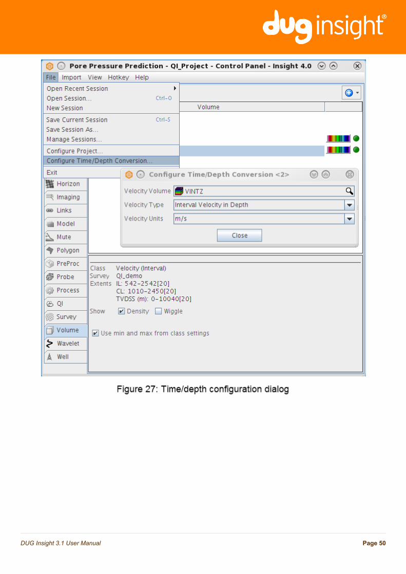
Time-depth configuration and velocity model selection

To assign the velocity for T/D conversion, select Configure Time/Depth Conversion (Figure 27) in the Filemenu of the Insight control panel. The selected velocity model will be used to convert between TWT and TVDthroughout Insight.

To assign the velocity volume for pore pressure prediction, under Pore Pressure tab, Default Velocity Modelselect:

• Velocity Model Source - as “Select Volume”• Velocity Volume - select from the the Insight “Volume” list• Verify the Velocity Type and Velocity Units.

Alternatively, you can use the volume selected for Insight depth conversion by setting Velocity Model Sourceto Inherit from T/D Settings.

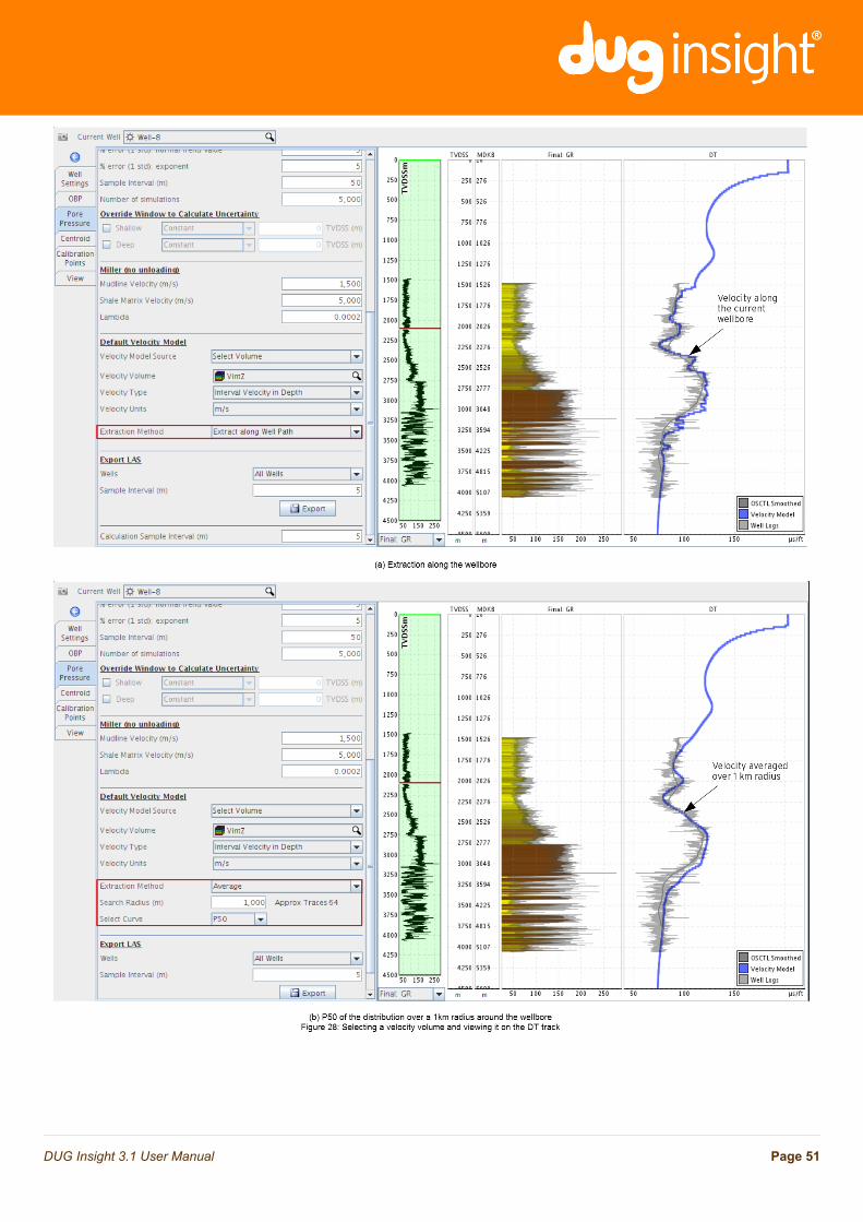
Once a velocity model is assigned, there are two options for “Extraction Method”:

• Extract along Well Path follows the wellbore path, straight or deviated.• Average requires a Search Radius (m) around the well (top hole location), from which velocity traces

are extracted and analysed for the “P10”, “P50”, and “P90”.

To see the velocity profile: under the View tab, Curves section, choose Velocity Model. It will appear on the“DT” track, converted to slowness along with wireline sonic logs and NCTL curves. Figure 28 shows anexample velocity trace extracted along the wellbore, both single and averaged.

Note: The selected Velocity Volume and Extraction Method can be overridden for any particular well underthe Well Settings tab. The (safest) default is to choose the Velocity Model Source as Inherit from PPSettings.


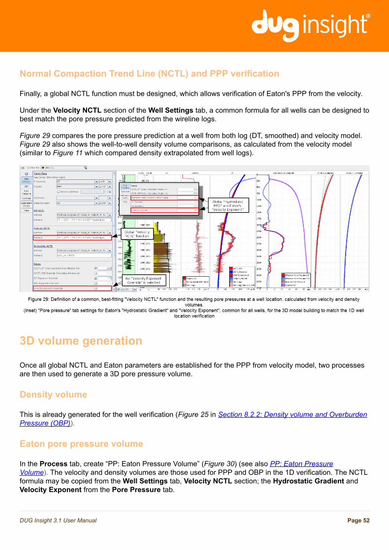
Normal Compaction Trend Line (NCTL) and PPP verification

Finally, a global NCTL function must be designed, which allows verification of Eaton's PPP from the velocity.

Under the Velocity NCTL section of the Well Settings tab, a common formula for all wells can be designed tobest match the pore pressure predicted from the wireline logs.

Figure 29 compares the pore pressure prediction at a well from both log (DT, smoothed) and velocity model.Figure 29 also shows the well-to-well density volume comparisons, as calculated from the velocity model(similar to Figure 11 which compared density extrapolated from well logs).

3D volume generation

Once all global NCTL and Eaton parameters are established for the PPP from velocity model, two processesare then used to generate a 3D pore pressure volume.

Density volume

This is already generated for the well verification (Figure 25 in Section 8.2.2: Density volume and OverburdenPressure (OBP)).

Eaton pore pressure volume

In the Process tab, create “PP: Eaton Pressure Volume” (Figure 30) (see also PP: Eaton PressureVolume). The velocity and density volumes are those used for PPP and OBP in the 1D verification. The NCTLformula may be copied from the Well Settings tab, Velocity NCTL section; the Hydrostatic Gradient andVelocity Exponent from the Pore Pressure tab.


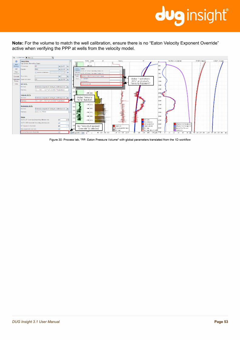
Note: For the volume to match the well calibration, ensure there is no “Eaton Velocity Exponent Override”active when verifying the PPP at wells from the velocity model.


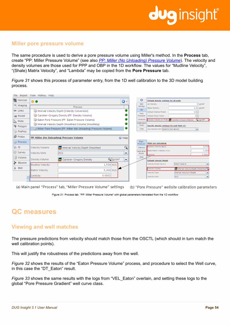
Miller pore pressure volume

The same procedure is used to derive a pore pressure volume using Miller's method. In the Process tab,create “PP: Miller Pressure Volume” (see also PP: Miller (No Unloading) Pressure Volume). The velocity anddensity volumes are those used for PPP and OBP in the 1D workflow. The values for “Mudline Velocity”,“(Shale) Matrix Velocity”, and “Lambda” may be copied from the Pore Pressure tab.

Figure 31 shows this process of parameter entry, from the 1D well calibration to the 3D model buildingprocess.

QC measures

Viewing and well matches

The pressure predictions from velocity should match those from the OSCTL (which should in turn match thewell calibration points).

This will justify the robustness of the predictions away from the well.

Figure 32 shows the results of the “Eaton Pressure Volume” process, and procedure to select the Well curve,in this case the “DT_Eaton” result.

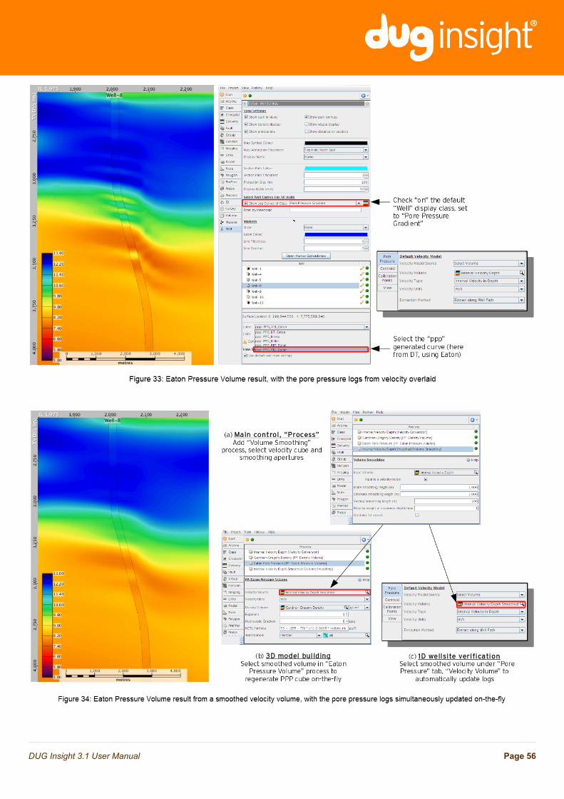
Figure 33 shows the same results with the logs from “VEL_Eaton” overlain, and setting these logs to theglobal “Pore Pressure Gradient” well curve class.


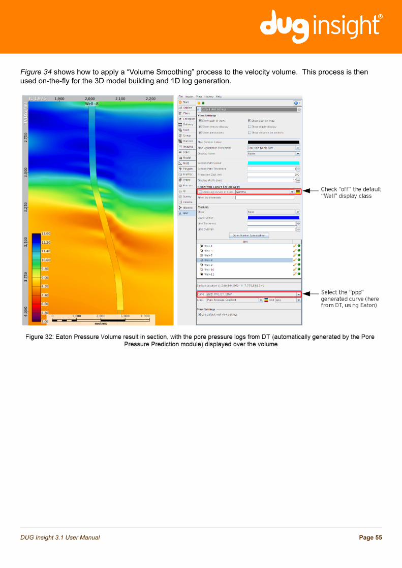
Figure 34 shows how to apply a “Volume Smoothing” process to the velocity volume. This process is thenused on-the-fly for the 3D model building and 1D log generation.


View and Export Options


Introduction

The 1D well calibration (Pore Pressure Prediction view) offers detailed controls on the track and curve views.

Most of these can be set from either the View tab, or by right clicking one of the display tracks, and choosingConfigure Track.

All generated curves can be exported to LAS file format.

“View” tab options


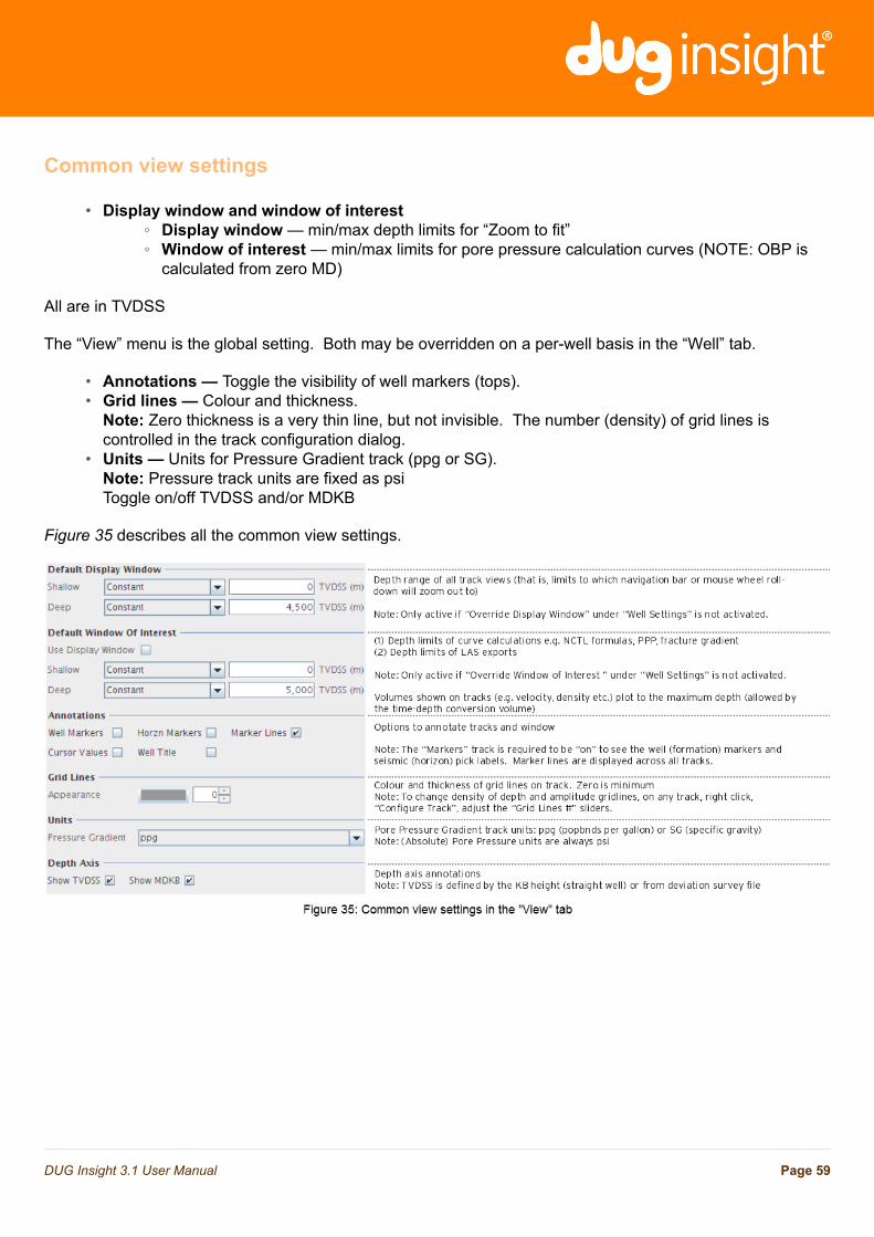
Common view settings

• Display window and window of interest◦ Display window — min/max depth limits for “Zoom to fit”◦ Window of interest — min/max limits for pore pressure calculation curves (NOTE: OBP is

calculated from zero MD)

All are in TVDSS

The “View” menu is the global setting. Both may be overridden on a per-well basis in the “Well” tab.

• Annotations — Toggle the visibility of well markers (tops).• Grid lines — Colour and thickness.

Note: Zero thickness is a very thin line, but not invisible. The number (density) of grid lines iscontrolled in the track configuration dialog.

• Units — Units for Pressure Gradient track (ppg or SG).Note: Pressure track units are fixed as psiToggle on/off TVDSS and/or MDKB

Figure 35 describes all the common view settings.


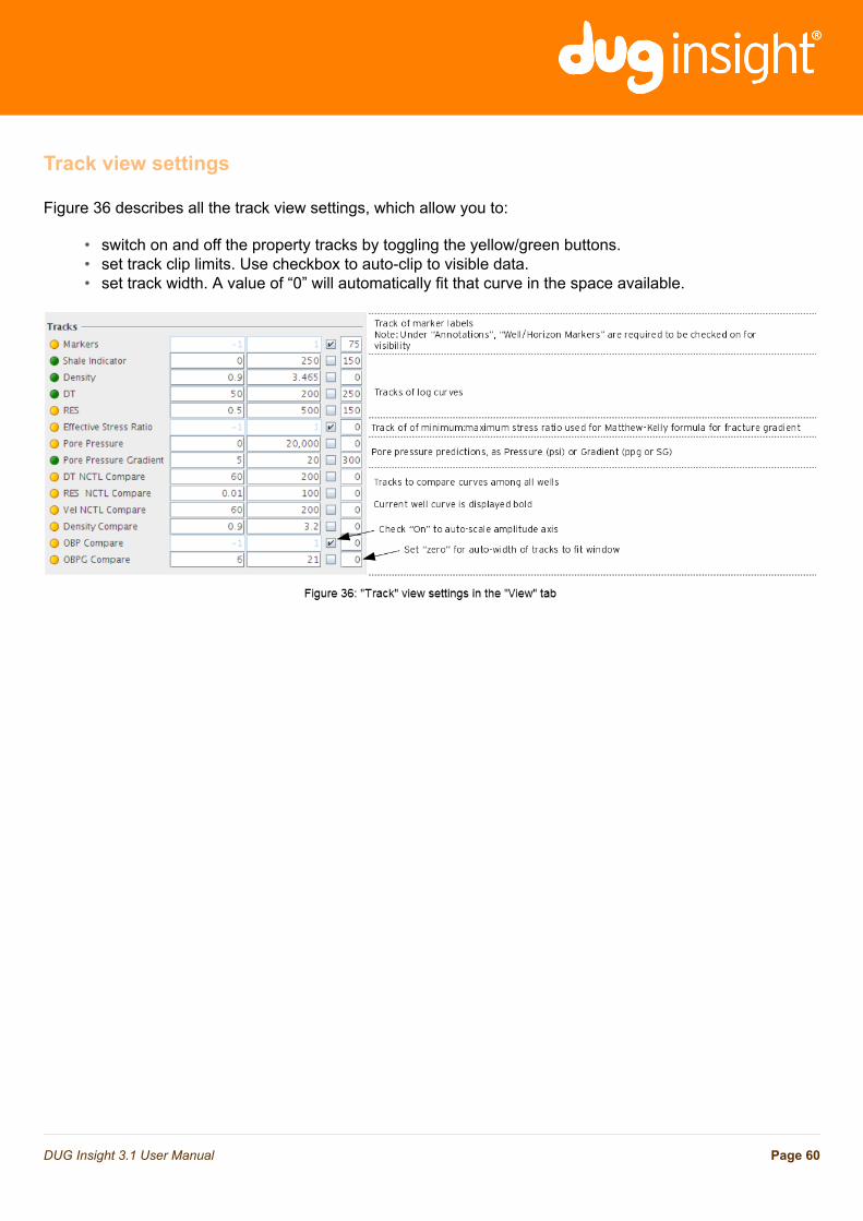
Track view settings

Figure 36 describes all the track view settings, which allow you to:

• switch on and off the property tracks by toggling the yellow/green buttons.• set track clip limits. Use checkbox to auto-clip to visible data.• set track width. A value of “0” will automatically fit that curve in the space available.


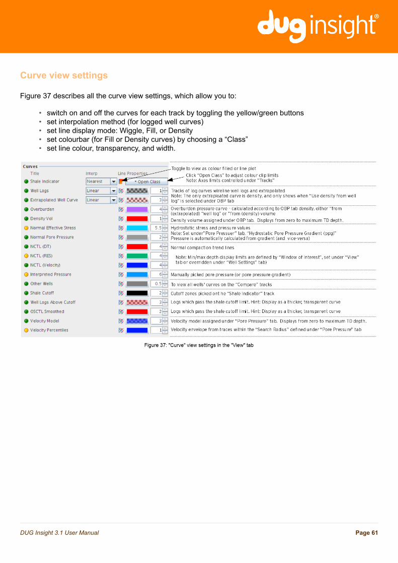
Curve view settings

Figure 37 describes all the curve view settings, which allow you to:

• switch on and off the curves for each track by toggling the yellow/green buttons• set interpolation method (for logged well curves)• set line display mode: Wiggle, Fill, or Density• set colourbar (for Fill or Density curves) by choosing a “Class”• set line colour, transparency, and width.


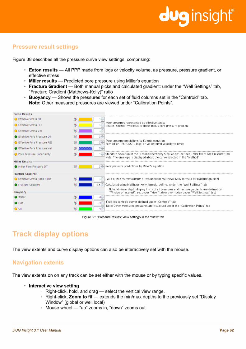
Pressure result settings

Figure 38 describes all the pressure curve view settings, comprising:

• Eaton results — All PPP made from logs or velocity volume, as pressure, pressure gradient, oreffective stress

• Miller results — Predicted pore pressure using Miller's equation• Fracture Gradient — Both manual picks and calculated gradient: under the “Well Settings” tab,

“Fracture Gradient (Matthews-Kelly)” ratio• Buoyancy — Shows the pressures for each set of fluid columns set in the “Centroid” tab.

Note: Other measured pressures are viewed under “Calibration Points”.

Track display options

The view extents and curve display options can also be interactively set with the mouse.

Navigation extents

The view extents on on any track can be set either with the mouse or by typing specific values.

• Interactive view setting◦ Right-click, hold, and drag — select the vertical view range.◦ Right-click, Zoom to fit — extends the min/max depths to the previously set “Display

Window” (global or well local)◦ Mouse wheel — “up” zooms in, “down” zooms out


◦ Left-click, hold, and drag — moves the entire track up or down (if not already zoomed tomaximum extents)

• Manual view setting◦ The overall Display limits are set via global or well “Display Window” in the tabs on the left.◦ To set specific values, right-click on a track and select Configure track; or see the Tracks

section in the View tab.


Curve view options

Right-click on a track and select Configure Track to choose all view options for a given track – Title, Rangeand Domain (linear/log), Depth range, Width, Legend, Grid Lines, and all Curve options.

The advantage of using the per-track configure dialog is that it shows only the curves and controls relevant tothis track, simplifying the display as shown in Figure 39.


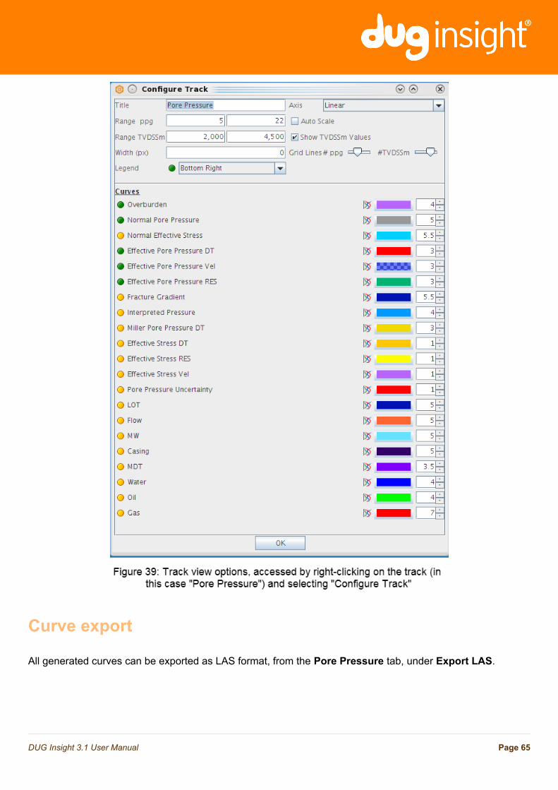
Curve export

All generated curves can be exported as LAS format, from the Pore Pressure tab, under Export LAS.


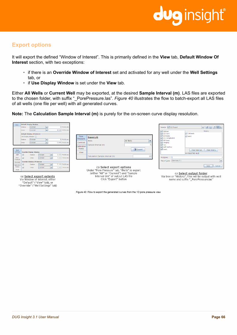
Export options

It will export the defined “Window of Interest”. This is primarily defined in the View tab, Default Window OfInterest section, with two exceptions:

• if there is an Override Window of Interest set and activated for any well under the Well Settingstab, or

• if Use Display Window is set under the View tab.

Either All Wells or Current Well may be exported, at the desired Sample Interval (m). LAS files are exportedto the chosen folder, with suffix “_PorePressure.las”. Figure 40 illustrates the flow to batch-export all LAS filesof all wells (one file per well) with all generated curves.

Note: The Calculation Sample Interval (m) is purely for the on-screen curve display resolution.


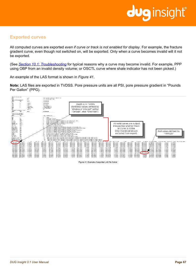
Exported curves

All computed curves are exported even if curve or track is not enabled for display. For example, the fracturegradient curve, even though not switched on, will be exported. Only when a curve becomes invalid will it notbe exported.

(See Section 10.1: Troubleshooting for typical reasons why a curve may become invalid. For example, PPPusing OBP from an invalid density volume; or OSCTL curve where shale indicator has not been picked.)

An example of the LAS format is shown in Figure 41.

Note: LAS files are exported in TVDSS. Pore pressure units are all PSI, pore pressure gradient in “PoundsPer Gallon” (PPG).


Workflow Hints and FAQsTroubleshooting

Common issues and solutions are shown below. For additional help, please email [email protected].


mailto:[email protected]

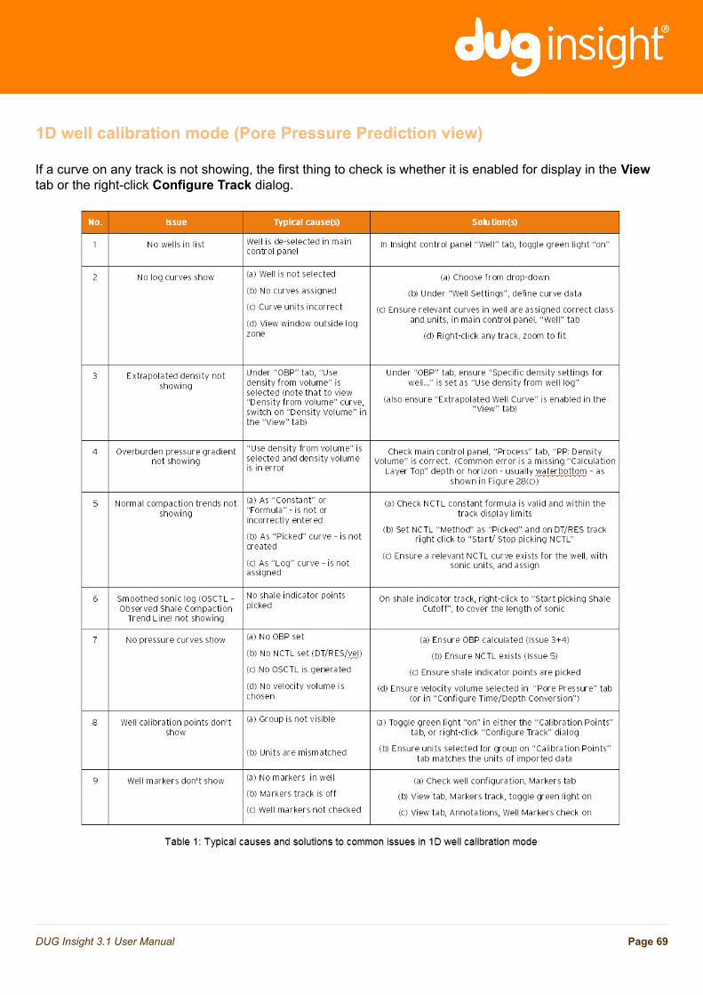
1D well calibration mode (Pore Pressure Prediction view)

If a curve on any track is not showing, the first thing to check is whether it is enabled for display in the Viewtab or the right-click Configure Track dialog.


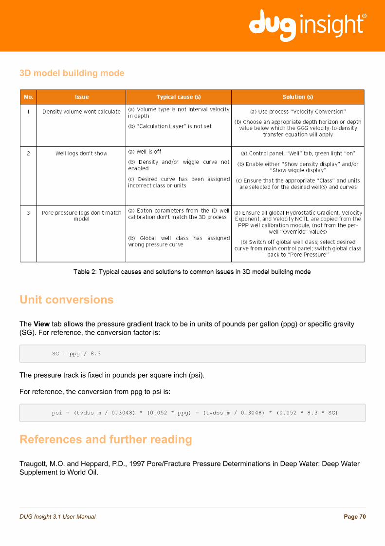
3D model building mode

Unit conversions

The View tab allows the pressure gradient track to be in units of pounds per gallon (ppg) or specific gravity(SG). For reference, the conversion factor is:

SG = ppg / 8.3

The pressure track is fixed in pounds per square inch (psi).

For reference, the conversion from ppg to psi is:

psi = (tvdss_m / 0.3048) * (0.052 * ppg) = (tvdss_m / 0.3048) * (0.052 * 8.3 * SG)

References and further reading

Traugott, M.O. and Heppard, P.D., 1997 Pore/Fracture Pressure Determinations in Deep Water: Deep WaterSupplement to World Oil.


van Ruth, P., Hillis, R. and Tingate, P., 2004, The origin of overpressure in the Carnarvon Basin WA -implications for pore pressure prediction, Petroleum Geoscience, 10, 247-257.

Yardley, G.S. and Swarbrick, R.E., 2001, Lateral Transfer: A source of additional overpressure: Marine andPetroleum Geology.

Zhang, J., 2011, Pore pressure prediction from well logs: Methods, modifications and new approaches, Earth-Science Reviews, 108, 50-63.


pore pressure predict

Documents