1

Porosity and Permeability Prediction through Forward Stratigraphic

Simulations Using GPMTM and PetrelTM: Application in Shallow

Marine Depositional Settings.

Daniel Otoo and David Hodgetts

Department of Earth and Environmental Sciences, University of Manchester, Manchester, M13 9PL, United Kingdom.

Correspondence to: Daniel Otoo (daniel.otoo@manchester.ac.uk)

Abstract

The forward stratigraphic simulation approach is applied to forecast porosity and permeability trends in

the Volve field subsurface model. Variograms and synthetic well logs from the forward stratigraphic

model were combined with known data to guide porosity and permeability distribution. Building a

reservoir model that fits data at different locations comes with high levels of uncertainty. Therefore, it is

critical to generate an appropriate stratigraphic framework to guide lithofacies and associated

petrophysical distribution in a subsurface model. The workflow adopted is in three parts; first, simulation

of twenty scenarios of sediment transportation and deposition using the geological process modeling

(GPMTM) software developed by Schlumberger. Secondly, an estimation of the extent and proportion of

lithofacies proportions in the stratigraphic model using the property calculator tool in PetrelTM. Finally,

porosity and permeability values were assigned to corresponding lithofacies-associations in the forward

stratigraphic model to produce a forward stratigraphic-based porosity and permeability model. Results

show a lithofacies distribution model, which depends on sediment diffusion rate, sea level variation, flow

rate, wave processes, and tectonic events. This observation is consistent with the natural occurrence,

where variation in sea level, sediment supply, and accommodation control stratigraphic sequences.

Validation wells, VP1 and VP2 located in the original Volve field model and the forward stratigraphic-

based models show a significant similarity, especially in the porosity models. These results suggest that

forward stratigraphic simulation outputs can be used together with geostatistical modeling workflows to

improve subsurface property representation in reservoir models.

2

Introduction 1

The distribution of reservoir properties such as porosity and permeability is a direct function of a complex 2

combination of sedimentary, geochemical, and mechanical processes (Skalinski & Kenter, 2014). The 3

impact of reservoir petrophysics on well planning and production strategies makes it imperative to use 4

reservoir modeling techniques that present realistic property variations via 3-D models (Deutsch and 5

Journel, 1999; Caers and Zhang, 2004; Hu & Chugunova, 2008). Typically, reservoir modeling requires 6

continued property modification until an appropriate match to subsurface data. Meanwhile, subsurface 7

data acquisition is expensive, thus restricts data collection and accurate subsurface property modeling. 8

Several studies, Hodgetts et al. (2004) and Orellana et al. (2014) have demonstrated how stratigraphic 9

patterns, and therefore petrophysical attributes in seismic data, outcrops, and well logs are applicable in 10

subsurface modeling. However, the absence of detailed 3-dimensional depositional frameworks to guide 11

property modeling inhibits this strategy (Burges et al. 2008). Reservoir modeling techniques with the 12

capacity to integrate forward stratigraphic simulation outputs with stochastic modeling techniques for 13

subsurface property modeling will improve reservoir heterogeneity characterization, because they more 14

accurately produce geological realism than the other modeling methods (Singh et al. 2013). The use of 15

geostatistical-based methods to represent spatial variability of reservoir properties has been in many 16

exploration and production projects (Kelkar and Godofredo, 2002). In the geostatistical modeling method, 17

an alternate numerical 3-D model (realizations) shows different property distribution scenarios that are 18

most likely to match well data (Ringrose & Bentley, 2015). However, due to cost reservoir modeling 19

practitioners continue to encounter the challenge of obtaining adequate subsurface data to deduce reliable 20

variograms for subsurface modeling, therefore introducing a significant level of uncertainty in reservoir 21

models (Orellena et al. 2014). The advantages of applying geostatistical modeling approaches to represent 22

reservoir properties in models are discussed in studies by Deutsch and Journel (1999), Dubrule, (1998). 23

A notable disadvantage is that the geostatistical modeling method tends to confine reservoir property 24

distribution to subsurface data and rarely produces geological realism to capture sedimentary events that 25

led to reservoir formation (Hassanpour et al. 2013). In effect, the geostatistical modeling technique does 26

3

not reproduce long-range continuous reservoir properties, which are essential for generating realistic 27

reservoir connectivity models (Strebelle & Levy, 2008). The forward stratigraphic simulation approach 28

was applied in this contribution to forecast lithofacies, porosity, and permeability in a reservoir model, 29

based on lessons from Otoo and Hodgetts (2019). A significant aspect of this work is using variogram 30

parameters from forward stratigraphic-based synthetic wells to simulate porosity and permeability trends 31

in the reservoir model. Forward stratigraphic modeling involves morphodynamic rules to replicate 3-32

dimensional stratigraphic depositional trends observed in data (e.g. seismic). Forward stratigraphic 33

modeling operates on the guiding principle that multiple sedimentary process-based simulations in a 3-D 34

framework will improve facies, and therefore petrophysical property distribution in a geological model. 35

The geological process modeling GPMTM software (Schlumberger, 2017), which operates on forward 36

stratigraphic simulation principles, replicates a depositional sequence to provide a 3-dimensional 37

framework to predict porosity, permeability in the study area. The reservoir interval under study is within 38

the Hugin formation. Studies by Varadi et al. (1998); Kieft et al. (2011) indicate that the Hugin formation 39

consists of a complex depositional architecture of waves, tidal, and fluvial processes. This knowledge 40

suggests that a single depositional model will not be adequate to produce a realistic lithofacies or 41

petrophysical distributions model of the area. Furthermore, the complicated Syn-depositional rift-related 42

faulting system, significantly influences the stratigraphic architecture (Milner and Olsen, 1998). 43

Therefore, the focus here is to produce a depositional sequence, which captures subsurface attributes 44

observed in seismic and well data to guide property modeling. 45

Study Area 46

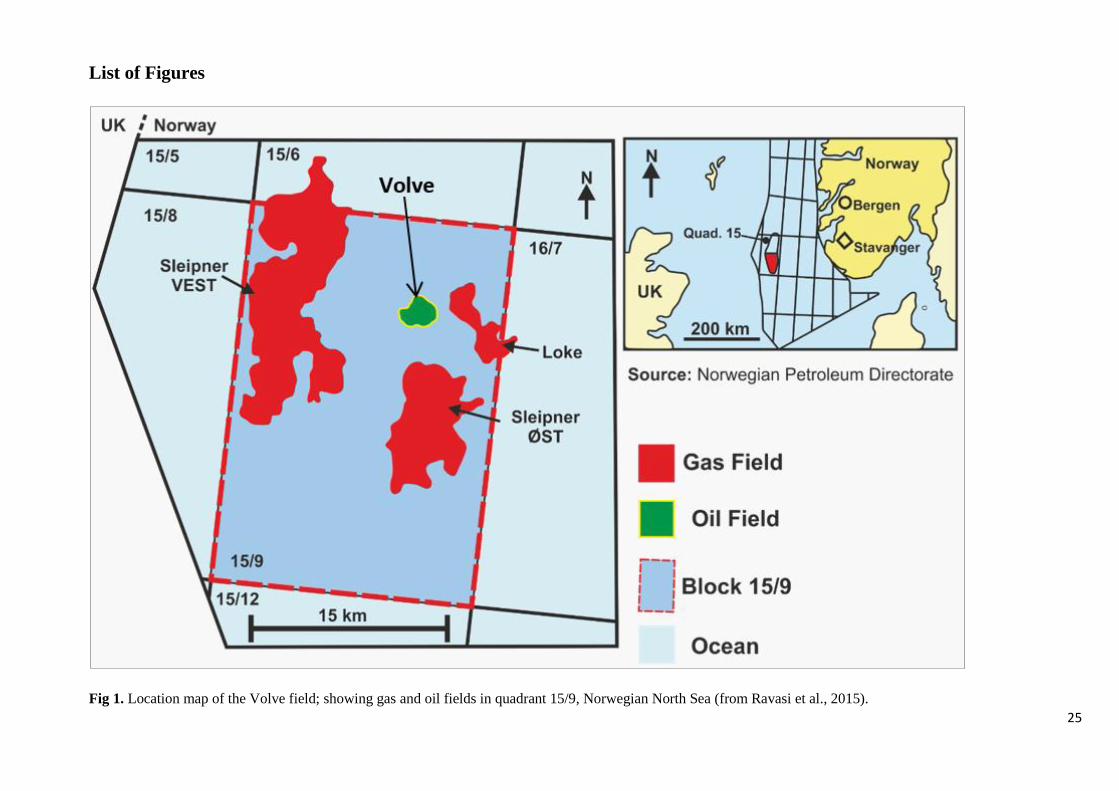
The Volve field (Figure 1), located in Block 15/9 south of the Norwegian North Sea, has the Hugin 47

Formation as the reservoir interval from which hydrocarbons are produced (Vollset and Dore, 1984). The 48

Hugin formation, which is Jurassic in age (late Bajocian to Oxfordian), is made up of shallow marine to 49

marginal marine sandstone deposits, coals, and a significant influence of wave events that tend to control 50

lithofacies distribution in the formation (Varadi et al. 1998; and Kieft et al. 2011). Studies by Sneider et 51

al. (1995) and Husmo et al. (2003) associate sediment deposition into the study area to rift-related 52

4

subsidence and successive flooding during a large transgression of the Viking Graben within the Middle 53

to Late Jurassic period. Also, Cockings et al. (1992), Milner and Olsen (1998) indicate that the Hugin 54

formation comprises of marine shoreface, lagoonal and associated coastal plain, back-stepping delta-55

plain, and delta front. However, recent studies by Folkestad and Satur (2006) also provide evidence of a 56

high tidal event, which introduces another dimension that requires attention in any subsurface modeling 57

task in the study area. The thickness of the Hugin formation is estimated between 5 m and 200 m, but can 58

be thicker off-structure and non-existent on structurally high segments due to post-depositional erosion 59

(Folkestad and Satur, 2006). 60

A summarised sedimentological delineation within the Hugin formation is derived based on studies by 61

Kieft et al. (2011). In Table 1, lithofacies-association codes A, B, C, D, and E represent bay fill units, 62

shoreface sandstone facies, mouth bar units, fluvio-tidal channel fill sediments, and coastal plain facies 63

units, respectively. Additionally, a lithofacies association prefixed code F, which consists of open marine 64

shale units, mudstone. Within it are occasional siltstone beds, parallel laminated soft sediment 65

deformation that locally develop at bed tops. The lateral extent of the code F lithofacies package in the 66

Hugin formation is estimated to be 1.7 km to 37.6 km, but the total thickness of code F lithofacies is not 67

known (Folkestad & Satur, 2006). 68

Data and Software 69

This work is based on the description and interpretation of petrophysical datasets in the Volve field by 70

Equinor. Datasets include 3-D seismic and a suite of 24 wells that consist of formation pressure data, core 71

data, petrophysical and sedimentological logs. Previous studies by Folkestad & Satur (2006) and Kieft et 72

al., (2011) in this reservoir interval show varying grain size, sorting, sedimentary structures, bounding 73

contacts of sediment matrix. Grain size, sediment matrix, and the degree of sorting will typically drive 74

the volume of the void created, and therefore the porosity and permeability attributes. Wireline-log 75

attributes such as gamma-ray (GR), sonic (DT), density (RHOB), and neutron-porosity (NPHI) 76

distinguish lithofacies units, stratigraphic horizons, and zones that are essential for building the 3-D 77

property model in Schlumberger’s PetrelTM software. Besides, this study also seeks to produce a realistic 78

5

depositional model like the natural stratigraphic framework in a shallow marine depositional setting. 79

Therefore, obtaining a 3-dimensional stratigraphic model that shows a similar stratigraphic sequence 80

observed in the seismic data allows us to deduce variogram parameters to serve as input in actual 81

subsurface property modeling. 82

Twenty forward stratigraphic simulations were produced in the geological process modeling (GPMTM) 83

software to illustrate depositional processes that resulted in the build-up of the reservoir interval under 84

study. By the fourth simulation, there was a development of stratigraphic patterns that shows similar 85

sequences as those observed in seismic, hence the decision to constrain the simulation to twenty scenarios. 86

Delft3D-FlowTM; Rijin & Walstra, (2003); DIONISOSTM; Burges et al. (2008) are examples of subsurface 87

process modeling software used in similar studies. The availability of the GPMTM software license and 88

the capacity to integrate stratigraphic simulation outputs in the property modeling workflow in PetrelTM 89

is the reason for using the geological process modeling software in this study. 90

Methodology 91

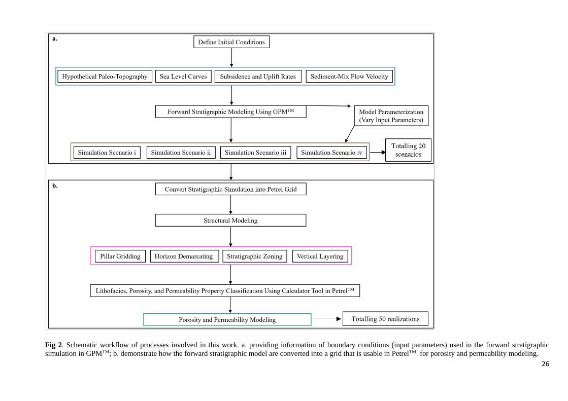
The workflow (Figure 2a) combines the stratigraphic simulation capacity of GPMTM in different 92

sedimentary processes and the property modeling tools in PetrelTM to predict the distribution of porosity 93

and permeability properties away from known data. This involves three broad: (i) forward stratigraphic 94

simulation in GPMTM (2019.1 version), (ii) lithofacies classification using the calculator tool in PetrelTM, 95

and (iii) porosity and permeability modeling in PetrelTM (2019.1 version). 96

Forward Stratigraphic Simulation in GPMTM 97

The GPMTM software consists of different geological processes to replicate sediment deposition in clastic 98

and carbonate environments. Kieft et al. (2011) in their work in this area, identified the influence of fluvial 99

and wave processes in the genetic structure of sediments in the Hugin formation. These geological 100

processes are very rapid, depending on accommodation generated by sea-level variation and or sediment 101

composition and flow intensity. The deposition of sediments into a geological basin and its response to 102

post-depositional sedimentary or tectonic processes are significant in the ultimate distribution of 103

6

subsurface lithofacies and petrophysics. Therefore, different input parameters for the forward simulation 104

to attain a stratigraphic output that fits existing knowledge of paleo-sediment transportation and 105

deposition into the study area (see Table 2). The forward simulation at all stages portrayed geological 106

realism concerning stratigraphic sequence, but it also revealed some limitations, such as instability in the 107

simulator when more than three geological processes run concurrently. Given this, the diffusion and 108

tectonic processes remained constant, whiles varying the steady flow, unsteady flow, and sediment 109

accumulation processes at each run. 110

Steady & Unsteady Flow Process 111

The steady flow process in GPM simulates flows that change slowly over a period, or sediment transport 112

scenarios where flow velocity and channel depth do not vary abruptly e.g., rivers at a normal stage, deltas, 113

and sea currents. The steady flow process can be specified to the desired setting in the “run sedimentary 114

simulation” dialog box in the PetrelTM software (version 2017.1 and above). Considering the influence of 115

fluvial activities during sedimentation in the Hugin formation, it is significant to capture its impact on the 116

resultant simulated output. A boundary condition is specified at the edges of the model structure to guide 117

sediment and fluid movement in the model. For example, where the boundary condition is an open flow 118

system, negative integers (values below zero) must be assigned to the edges of the hypothetical paleo-119

surface to allow water to enter and leave the area of interest. 120

The unsteady flow process can simulate periodic flows and run for a limited time; for example, in 121

turbidites where the velocity of flow and depth changes abruptly over time. The unsteady flow process 122

algorithm applies several fluid elements driven by gravity and friction against the hypothetical 123

topographic surface. In Otoo and Hodgetts (2019), is an account of how the unsteady process in GPMTM 124

attains realistic distribution of lithofacies units in a turbidite fan system. The steady and unsteady flow 125

processes are based on simplified Navier-Stokes equations to represent flows in channels and pathways 126

that have irregular cross-sections and or channels that converge as tributaries or diverge as distributaries 127

such as turbidite flow. The simplified Navier-Stokes comprises of two key parameters that partly rely on 128

channel geometry and flow velocity. The Navier-Stokes equation combines the continuity equation (2) 129

7

and the momentum equation (3) to generate the equation on which the steady and unsteady flow processes 130

evolve. 131

The continuity equation integrates the conservation of mass: 132

𝜕𝜌

𝜕𝑡 + 𝛻.𝜌q = 0 (1) 133

Where 𝜌 is fluid density, t is time, and q the flow velocity vector. 134

The equation that shows the changes in momentum by the fluid: 135

p.(𝜕𝑞

𝜕𝑡+ (𝑞. 𝛻)𝑞) = −𝛻𝜌 + 𝛻. 𝜇𝑈 + 𝜌(𝑔 + 𝛺𝑞) (2) 136

Where P is pressure, t is time, μ is fluid viscosity, and U is the Navier Stokes tensor. 137

Keeping density (𝜌) and viscosity (μ) as constant, a simple flow equation is obtained: 138

𝜕𝑞

𝜕𝑡 + (q .𝛻)q = -𝛻Φ + v𝛻²q + g (3) 139

Where, Φ is the ratio of pressure to constant density (i.e. P/𝜌), and v is the kinematic viscosity (i.e. μ/𝜌) 140

The solution of the framework formed in (3) is completely obtained by specifying various boundary 141

conditions that are used in the steady and or unsteady flow processes. 142

A full description of equations that form the building block for sediment movement under steady and 143

unsteady flow processes in the simulator is available in Tetzlaff & Harbaugh (1989). 144

Sediment Diffusion Process 145

The diffusion process can effectively replicate sediment movement from a higher slope (source location) 146

and its deposition into a lower elevation of the model area. Sediment movement in the diffusion process 147

is through erosion and transportation processes that are driven by gravity. Sediment diffusion runs on the 148

assumption that sediments are transported downslope at a proportional rate to the topographic gradient, 149

making fine-grained sediments easily transportable than coarse-grained sediments. Sediment diffusion 150

depends on three parameters: (i) sediment grain size and turbulence in the flow (ii) diffusion coefficient, 151

8

and (iii) diffusion curve that serves as a unitless multiplier in the algorithm. Based on Dade & Friend 152

(1998); and Zhong (2011), a mathematical summary of the influence these factors have on the resultant 153

diffusion profile is derived. Considering that the grain size for each sediment component (coarse sand, 154

fine sand, silt, and clay) are known, the assumption is that these particles have a uniform diameter (D) in 155

the flow mix. In that case, external fore (Fe), which consist of drag, lift, virtual mass, and Basset history 156

force is given as: 157

Fe = αeMe + αeΦD.𝑈𝑓𝑖−𝑈𝑒𝑖

𝑇𝑝 (4) 158

Me is the resultant force of other forces with the exception of drag force, Tp stokes relation time, expressed 159

as: Tp = 𝜌𝜌D²/(18𝜌fVf), with 𝜌f and Vf as density and viscosity of fluid respectively. ΦD is a coefficient 160

that accounts for the non-linear dependence of drag force on grain slip Reynolds number (Rp). 161

ΦD = Rp

24𝐶𝐷 (5), with CD sediment grain coefficient. 162

With the flow component in place, the diffusion coefficient (Di) is deduced from the Einstein equation. 163

Using an assumption that the diffusion coefficient decreases with increasing grain size and rise in 164

temperature, and that the coefficient f is known, the expression for Di is: 165

Di = 𝐾𝐵.𝑇

𝑓 (6) 166

Meanwhile, f is a function of the dimension of the spherical particle involved at a particular time (t). In 167

accounting for f, the equation for Di changes into: 168

Di = 𝐾𝐵.𝑇

6.𝜋.ղ𝑜.𝑟 (7) 169

The rate diffusion of diffusion relative to topography in the simulator is achieved through; 170

𝜕𝑧

𝜕𝑡= 𝐷𝑖∇²z (8) 171

where z is topographic elevation, k the diffusion coefficient, t for time, and ∇²z is the laplacian. 172

9

Sediment Accumulation 173

In GPMTM, sediment source can be set to a point location or considered to emanate from a whole area. 174

Sediment accumulation represents sediment deposition through an areal source. For example, where a 175

lithology is distribution is invariable, the sediment accumulation process can replicate such a depositional 176

scenario. The areal input rates for each sediment type (coarse grained, fine grained sediments) use the 177

value of the surface at each cell in the model grid and multiply it by a value from a unitless curve at each 178

time step in the simulation to estimate the thickness of sediments accumulated or eroded from a cell in 179

the model. Based on Tetzlaff & Harbaugh (1989), the equation for estimating sediment accumulation is 180

given: 181

(H – Z)𝐷𝑙𝐾𝑠

𝐷𝑡= 𝑓(𝑄, 𝛻𝐻, 𝛻𝑍, 𝐿, 𝐹, 𝐾𝑠 , 𝑘(𝑍)) (9) 182

Where; 183

H is the free surface elevation to sea level, Z is the topographic elevation for sea level, Ksis the sediment 184

type, lks, is the volumetric sediment concentration of a specific type (k), L is the vector that defines 185

sediment concentration of each type, F is the matrix of coefficients that define each sediment type, and t 186

is the time. 187

Sediment accumulation relies on (i) basin geometry and tectonics (Bajpai et al. 2001) (ii) erosion and 188

volume of sediment transported (Cheng, et al. 2018), (iii) prevailing accommodation. 189

Based on Cheng et al. (2018), sediment accumulation over a period (Ar) is: 190

Ar = Ver – Ves (10) 191

Ves, is the total volume of sediments that may escapes from the basin. Ver is the total volume of sediments 192

eroded into the basin. Ver = Aer x Rer x t; where Aer is the average erosion area, Rer is the average erosion 193

rate, and t, time. 194

Because source position for the sediment accumulation process is areal, the volume of sediments 195

accumulated in a specific layer (k) in the basin; excluding porosity, is expressed as: 196

10

Ar = ∑ 𝐴𝑟𝑘 𝑛𝑘=1 (11) 197

Taking into account the impact of porosity (ϕ) in this process, the equation for the sediment accumulation 198

is: 199

Ar = ∑ [(1 − 𝜙0 ∗ 𝑒−𝑐∗𝑧𝑘) 𝑋 𝑉𝑜𝑏𝑠𝑒𝑟𝑣𝑒𝑑𝑘 𝑛

𝑘=1 (12) 200

Where; Vobservedk is the volume of sediment and porosity observed in a specific layer (k), ϕ0 is the surface 201

porosity, c is the porosity-depth coefficient (after Sclater & Christie, 1980), and Zk is the average depth 202

of the layer k. 203

Boundary Conditions for Forward Stratigraphic Simulation 204

Realistic reproduction of stratigraphic patterns in the model area requires input parameters (initial 205

conditions), such as paleo-topography, sea-level curves, sediment source location, and distribution curve, 206

tectonic event maps (subsidence and uplift), and sediment mix velocity. The application of these input 207

parameters in GPMTM and their impact on the resultant stratigraphic framework is below. 208

Hypothetical Paleo-Surface: The hypothetical paleo-topographic for the stratigraphic simulation is from the 209

seismic data (Figure 3), using the assumption that the present day stratigraphic surface (paleo shoreline in Figure 210

4a) occurred as a result of basin filling over geological time. Since the surface obtained from the seismic section 211

have undergone various phases of subsidence and uplifts, it is significant to note that the paleo topographic surface 212

used in this work does not represent an accurate description of the basin at the period of sediment deposition; thus 213

presenting another level of uncertainty in the simulation. To derive an appropriate paleo-topographic for this 214

task, five paleo topographic surfaces (TPr) were generated, by adding or subtracting elevations from the 215

inferred paleo topographic surface (see Figure 4g) using the equation: 216

TPr = Sbs + EM (13) 217

where, Sbs is the base surface scenario (in this instance, scenario 6), and EM an elevation below and 218

above the base surface. 219

The paleo-topographic surface in scenario 3 (figure 4d) is selected because it produced a stratigraphic 220

sequences that fit the depositional patterns interpreted from the seismic section (Figure 5d). 221

11

Sediment Source Location: Based on regional well correlations in Kieft et al. 2011, and seismic 222

interpretation of the basin structure, the sediment entry point is placed in the north-eastern section of the 223

hypothetical paleo-topography surface. The exact sediment entry point into this basin is unknown, so 224

three entry points were placed at a 4 km radius around the primary location (Figure 3c) to capture possible 225

sediment source locations in the model area. The source position is a positive integer (values greater than 226

zero) to enable sediment movement to other parts of the topographic surface. 227

Sea Level: The sea-level curve is deduced from published studies and facies description in shallow marine 228

depositional environments (e.g. Winterer and Bosellini, 1981). To sea level was constrained 30 m for 229

short simulation runs (5000 to 20000 years), but varied with the increasing duration of the simulation (see 230

Table 2). The peak sea-level in the simulation depicts the maximum flooding surface (Figure 5d), and 231

therefore the inferred sequence boundary in the geological process model. 232

Diffusion and Tectonic Event Rates: The sediment mix proportion, diffusion rate, and tectonic event 233

functions are from studies such as Walter, (1978), Winterer and Bosellini, (1981), and Burges et al., 234

(2008). The diffusion and tectonic event rates were increased or reduced to produce a stratigraphic model 235

that fit our knowledge of basin evolution in the study area. For example, in scenario 1 (Figure 6a), the 236

early stages of clinoform development show resemblance to interpreted trends in the seismic section 237

(Figure 3b). The process commenced with a diffusion coefficient of 8 m2/a, but it varied at each scenario 238

to obtain diffusion coefficients to improve the model. Excluding the initial topography (Figure 4d), input 239

parameters in geological processes such as wave events, steady/unsteady flow, diffusion, and tectonic 240

events used curve functions to provide variations in the simulation. 241

The sensitivity of input parameters in the forward stratigraphic simulation is notable when there is a 242

change of value in sediment diffusion, and tectonic rates or dimension of the hypothetical topography. 243

For example, a change in sediment source position affects the extent and depth of sediments deposition 244

in the simulation. Shifting the source point to the mid-section of the topography (the mid-point of the 245

topography in a basin-ward direction) resulted in the accumulation of distal elements identical to turbidite 246

12

lobe systems. This output is consistent with morphodynamic experiments by de Leeuw et al. (2016), 247

where sediment discharge from the basin slope leads to the build-up of basin floor fan units. 248

Property Classification in Stratigraphic Model 249

In our opinion, the most appropriate output is the stratigraphic model in Figure 5d. This point of view is 250

because, compared to the depositional description in studies such as Folkestad and Satur (2006); Kieft et 251

al. (2011), and the seismic interpretation presents a similar stratigraphic sequence. Sediment distribution 252

in each time step of the simulation was stacked into a single zone framework to attain a simplified model. 253

This strategy assumes that sedimentary processes that lead to the final build-up of genetic related units 254

within zones of the model will not vary significantly over the simulation period. The stratigraphic model 255

(Figure 5d) was converted into a 3-D format (20 m x 20 m x 2 m grid cells) for the property modeling in 256

PetrelTM. 257

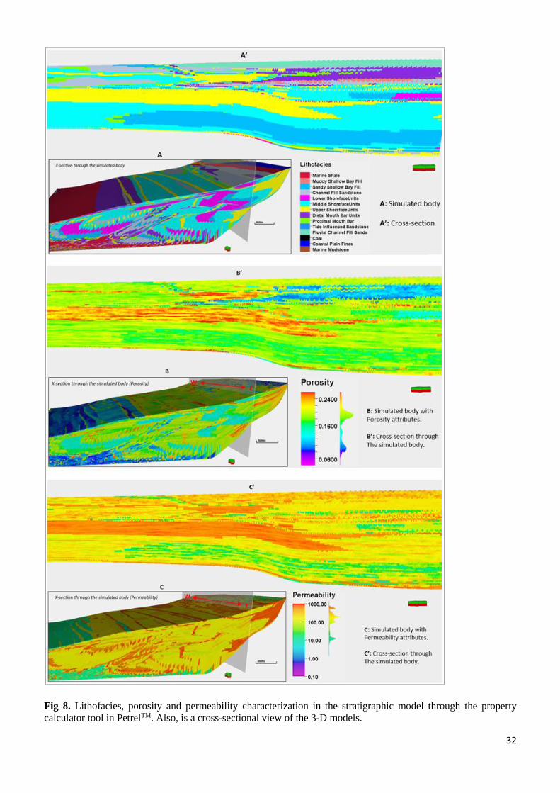
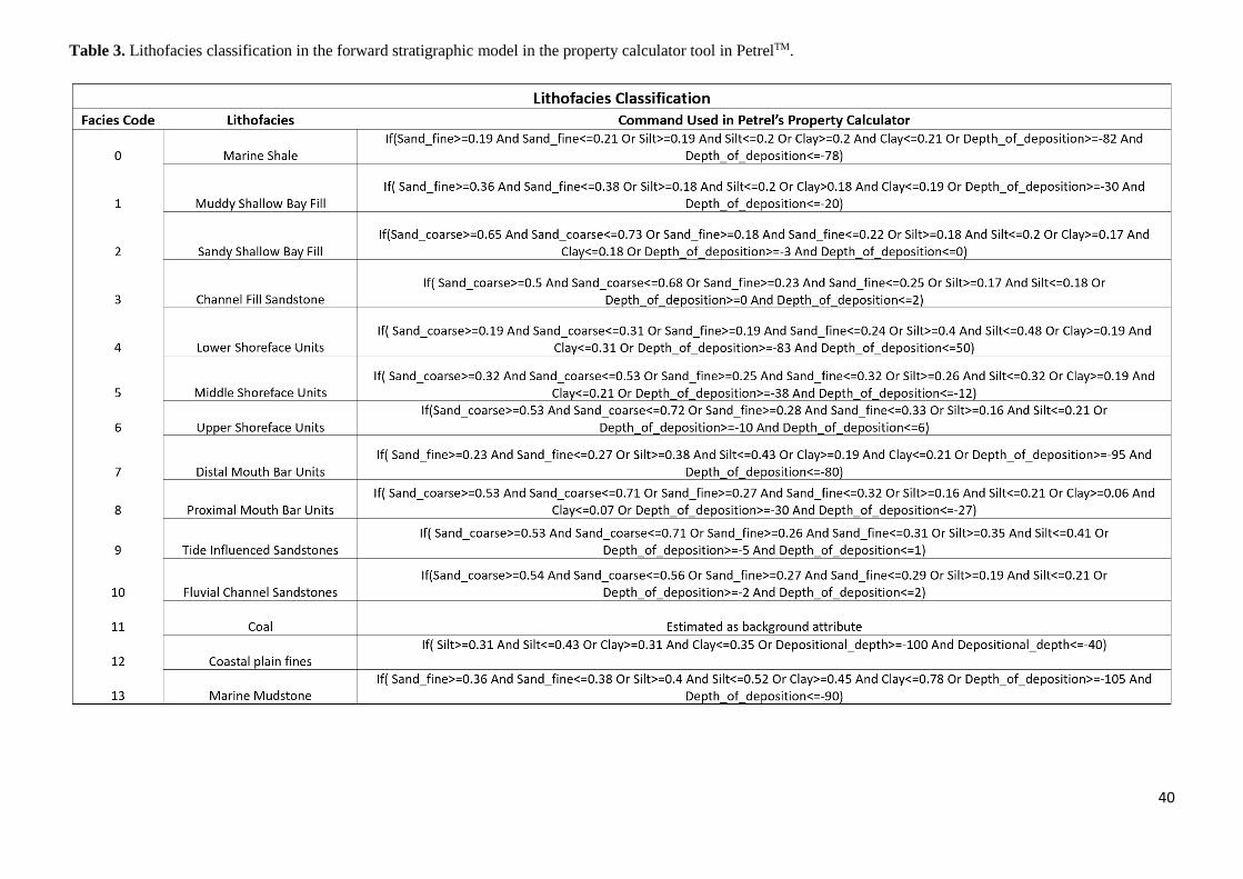
Facies, porosity, and permeability representation in the stratigraphic model was done via a rule based 258

approach in PetrelTM (see Table 3). The classification is driven by depositional depth, geologic flow 259

velocity, and sediment distribution patterns as indicated in Figure 7. Lithofacies representation in the 260

stratigraphic model relied on the sediment grain size pattern and proximity to sediment source. For 261

example, shoreface lithofacies units are medium-to-coarse grained sediments, which accumulate at a 262

proximal distance to the sediment source. In contrast, mudstone units are confined to fine-grained 263

sediments in the distal section of the simulation domain. 264

Using knowledge from published studies by Kieft et al. (2011) and wireline-log attributes such as gamma 265

ray, neutron, sonic, and density logs, porosity and permeability variations in the stratigraphic model are 266

estimated (Table 1). In previous studies on the Sleipner Øst, and Volve field (Equinor, 2006; Kieft et al. 267

2011), shoreface deposits make up the best reservoir units, whiles lagoonal deposits formed the worst 268

reservoir units. With this guide, shoreface sandstone units and mudstone/shale units in the forward 269

stratigraphic model are best and worst reservoir units respectively. The porosity and permeability values 270

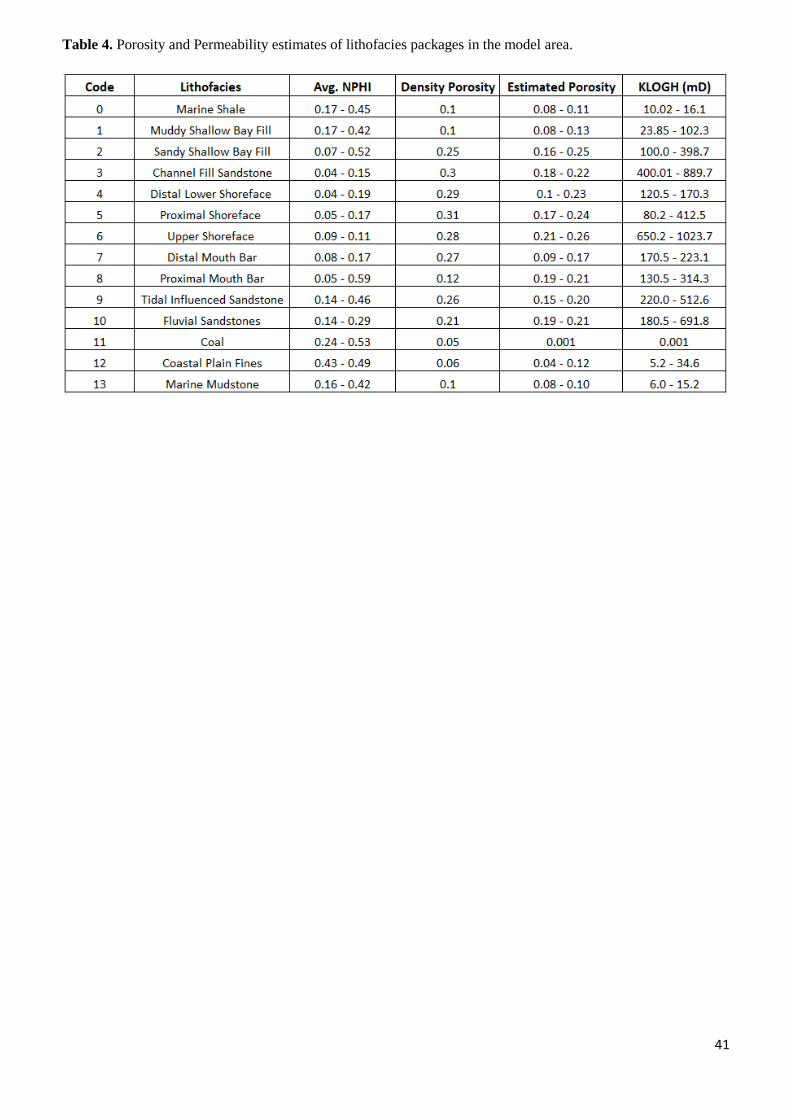
in Table 4 are from equations in Statoil’s petrophysical report of the Volve field (Equinor, 2016): 271

13

Øer = ØD + α . (NPHI - ØD) + β (14) 272

where Øer is the estimated porosity range, ØD is density porosity, α and β are regression constants; ranging 273

between -0.02 – 0.01 and 0.28 – 0.4 respectively, NPHI is neutron porosity. In instances where NPHI 274

values for lithofacies units is not available from the published references, an average of 0.25 was used. 275

KLOGHer = 10(2 + 8 * PHIF – 5 * VSH) (15) 276

where KLOGHer is the estimated permeability range, VSH is the volume of clay/shale in the lithofacies 277

unit, and PHIF, the fractured porosity. The VSH range between 0.01 – 0.12 for the shoreface units, and 278

0.78 – 0.88 for lagoonal deposits. 279

Property Modeling in PetrelTM 280

The workflow (Figure 2b) used for subsurface property modeling in PetrelTM is applied to represent 281

lithofacies, porosity, and permeability properties in the stratigraphic model. These processes involve: 282

(1) Structure modeling: identified faults within the study area are modeled together with interpreted 283

surfaces from seismic and well correlation to generate the main structural framework, within 284

which the property model is built. Here, fault pillars and connecting fault bodies are linked to 285

obtain the kind of fault framework interpreted from the seismic data. 286

(2) Pillar gridding: building a “grid skeleton” made up of a top, middle and base architectures. 287

Typically, pillars join corresponding corners of every grid cell of the adjacent grid to form the 288

foundation for each cell within the model. The prominent orientation of faults (I-direction) within 289

the model area was in an N-S and NE-SW direction, so the “I-direction” was set to NNE-SSW to 290

capture the general structural description of the area. 291

(3) Horizons, Zones, and Vertical Layering: stratigraphic horizons and subdivisions (zones) delineate 292

the geological formation’s boundaries. As stratigraphic horizons are introduced into the model 293

grid, the surfaces are trimmed iteratively and modified along faults to correspond with 294

displacements across multiple faults. Vertical layering shows the thicknesses and orientation 295

between the layers of the model. Layers refers to significant changes in particle size or sediment 296

14

composition in a geological formation. Using a vertical layering scheme makes it possible to honor 297

the fault framework, pillar grid, and horizons. A constant cell thickness of 1 m is used in the model 298

to control the vertical scale of lithofacies, porosity, and permeability modeling. 299

(4) Upscaling: involves the substitution of smaller grid cells with coarser grid cells. Here, log data is 300

transformed from 1-dimensional to a 3-dimensional framework to evaluate which discrete value 301

suits selected data point in the model. One advantage of the upscaling procedure is to make the 302

modeling process faster. 303

Porosity and Permeability Modeling 304

The Volve field porosity and permeability model from Equinor are adopted as the base (reference) model. 305

The model, which covers 17.9 km2 was generated with the reservoir management software (RMS), 306

developed by Irap and Roxar (EmersonTM). The petrophysical model has a grid dimension of 108 m x 307

100 m x 63 m and was compressed by 75.27% of cell size from an approximated cell size of 143 m x 133 308

m x 84 m. To achieve a comparable model resolution as the Volve field porosity and permeability model, 309

the forward stratigraphic output, which had an initial resolution of 90 m x 78 m x 45 m, is upscaled to a 310

grid of 107 m x 99 m x 63 m. Variograms being a critical aspect of this work, we submit two options to 311

extrapolate variogram parameters from the forward stratigraphic-based porosity and permeability models. 312

In Option 1, the porosity and permeability values were assigned to the synthetic lithofacies wells that 313

correlate with known facies-association in the study area (see Table 4). The pseudo wells comprising 314

porosity and permeability are situated in-between well locations to guide porosity and permeability 315

simulation in the model. For option 2, the best-fit forward stratigraphic model changes by assigning 316

porosity and permeability attribute using the general stratigraphic orientation captured in the seismic data 317

(NE-SW; 240⁰). Porosity and permeability pseudo (synthetic) logs were then extracted from the forward 318

stratigraphic output to build the porosity and permeability models (Figure 8). Porosity modeling is 319

through normal distribution, whiles the permeability models were produced using a log-normal 320

distribution and the corresponding porosity property for collocated co-kriging. 321

15

Considering that vertical trends in options 1 and 2 will be similar within a sampled interval, option 2 322

presented a viable 3-D representation of property variations in the major and minor directions of the 323

forward stratigraphic model. Ten synthetic wells (SW), ranging between 80 m and 120 m in total depth 324

(TD), are positioned in the forward model to capture the vertical distribution of porosity-permeability at 325

different sections of the forward stratigraphic-based models. 326

The synthetic wells (Figure 9 c) with porosity and permeability data were upscaled, and distributed into 327

the original structural model using the sequential Gaussian simulation method. The synthetic wells 328

derived from the stratigraphic model served as an additional control for porosity and permeability 329

modeling in the Volve field. Because the variogram-based modeling approach is efficient in subsurface 330

data conditioning, this idea presents an opportunity to get more wells at no additional cost to control 331

porosity and permeability distribution. The variogram model (Figure 10) of dominant lithofacies units in 332

the stratigraphic model served as a guide in estimating variogram parameters for porosity and 333

permeability modeling. The variogram has major and minor range of 1400 m and 400 m respectively, and 334

an average sill value of 0.75. Six out of fifty model realizations that show some similarity to the original 335

porosity and permeability model formed the basis of our analysis (Figure 11). The selection of six 336

realizations was on a visual and statistical comparison of zones in the original Volve field model and the 337

stratigraphic-based porosity/permeability model. The statistical approach involved summary statistics 338

from the reference model and the stratigraphic-based porosity/permeability model. In contrast, the visual 339

evaluation compared the geological realism of forward stratigraphic-based realizations to the base model. 340

Results 341

The stratigraphic model in stage 4 (Figure 5d iv) shows the final geometry after 700,000 years of 342

simulation time. The initial stratigraphic simulation produced a progradation sequence with foreset-like 343

features (Figure 5d i) and a sequence boundary, which separates the initial simulated output from the 344

next prograding phase (Figure 5d ii). An aggradational stacking pattern commences and becomes 345

prominent in stage 3 (Figure 5d iii). These aggradational sequences observed in the forward stratigraphic 346

16

model are consistent with natural events where sediment supply matchup with accommodation due to 347

sea-level rise within a geological period (Muto and Steel, 2000; Neal and Abreu, 2009). 348

Impact of the forward stratigraphic simulation on porosity and permeability representation in the reservoir 349

model is evident by comparing its outcomes to the Volve field porosity and permeability models by using 350

two synthetic well (VP1 and VP2); sampled at a 5 m vertical interval. Taking into account the fact that 351

the Volve field petrophysical model (Figure 11a) went through various phases of history matching to 352

obtain a model to improve well planning and production strategies, it is reasonable to assume that porosity 353

and permeability distribution in the petrophysical model will be geologically realistic and less uncertain. 354

This view formed the basis for using the porosity and permeability models developed by Equinor as a 355

reference for comparing outputs in the stratigraphic model. Table 5a shows an almost good match in 356

porosity at different intervals in the forward stratigraphic-based models (i.e. R14, R20, R26, R36, R45, 357

and R49). An analysis of the well logs in the model area shows that a large proportion of reservoir porosity 358

is between 0.18 – 0.24. Also, the analysis of the forward stratigraphic-based porosity model is consistent 359

with the porosity range in the Volve field model (see Figure 12). 360

A notable limitation with this approach is the assumption that variogram parameters and stratigraphic 361

inclination within zones remained constant throughout the simulation. The difference in permeability 362

attributes between the original permeability model and the forward stratigraphic-based type is the 363

application of other measured parameters in the original model (Table 5b). Typically, a petrophysical 364

model like the Sleipner Øst and Volve field model will factor in other datasets such as special core analysis 365

(SCAL) and level of cementation, which enhances reservoir petrophysics assessment. Bearing in mind 366

that the forward stratigraphic model did not involve some of this additional information from the 367

reservoir, it is practicable to suggest that results obtained in the forward stratigraphic-based porosity and 368

permeability models have adequately conditioned to known subsurface data. 369

17

Discussion 370

Results show the influence of sediment transport rate (or diffusion rate), initial basin topography, and 371

sediment source location on the stratigraphic simulation in in GPMTM. Compared to studies such as Muto 372

& Steel (2000) and Neal & Abreu (2009), we observed that a variation in sea-level controls the volume 373

of sediment that is retained or transported further into the basin, therefore controlling the resultant 374

stratigraphic sequences. In related work, Burges et al. (2008) suggest that a sediment-wedge topset width 375

connects directly to the initial bathymetry, in which the sediment-wedge structure develops, and the 376

correlation between sediment supply and accommodation rate. This opinion is in line with observations 377

in this study, where the initial sediment deposit controls the geometry of subsequent phases of depositions 378

in the hypothetical basin. The uncertainty of initial conditions used in this work led to the generation of 379

multiple forward stratigraphic scenarios to account for the range of bathymetries that may have influenced 380

sediment transportation to form the present-day reservoir units in the Volve field. 381

The simulation produced well-defined sloping depositional surfaces in a stratigraphic architecture 382

(clinoforms) and sequence boundaries that depict patterns seen in the seismic data. In their work, Allen 383

and Posamentier (1993); Ghandour and Haredy (2019) explained the importance of sequence stratigraphy 384

in lithofacies characterization, and therefore petrophysical property distribution in sedimentary systems. 385

Also, sediment deposition into a geological basin in the natural order is controlled by mechanical and 386

geochemical processes that modify petrophysical attributes (Warrlich et al. 2010); therefore, using 387

different geological processes and initial conditions to generate depositional scenarios in 3-dimension 388

provides a framework to analyse property variations in a hydrocarbon reservoir. The approach produces 389

a porosity-permeability model comparable to the original petrophysical model using synthetic porosity 390

and permeability logs from the forward stratigraphic model as input datasets. As mentioned, this work 391

did not include variations in the layering scheme that develops in different zones of the stratigraphic 392

model. Under this circumstance, there is a possibility to overestimate and or underestimate porosity and 393

permeability property in some sampled intervals in the validation wells. Therefore, we suggest that the 394

forward stratigraphic simulation outputs such as the example presented in this contribution serve as 395

18

additional data to understand sediment distribution patterns and associated vertical and horizontal 396

petrophysical trends in the depositional environment, and not as absolute conditioning data in subsurface 397

property modeling. 398

The assumptions made concerning the type of geological processes and input parameters in the 399

stratigraphic simulation certainly differ from what existed during sediment deposition. So, applying 400

stratigraphic models that fit a basin-scale description to a relatively smaller scale reservoir presents 401

another level of uncertainty in the approach. This finding agrees with Burges et al., (2008), where they 402

indicate that the diffusion geological process simulation fits the description of large-scale sediment 403

transportation. This view further buttresses the point that integrating forward stratigraphic simulation into 404

a well-scale framework has a high chance of producing outcomes that deviate from the real-world 405

subsurface description. In line with observations in Bertoncello et al. (2013); Aas et al. (2014); and Huang 406

et al. (2015) in relations to limitations in the forward stratigraphic simulation method, it is advisable to 407

use its outputs cautiously in reservoir modeling; as such outputs from forward stratigraphic models could 408

lead to an increase in property representation bias in a model. 409

The correlation between reservoir lithofacies and petrophysics, and its prediction through reservoir 410

models, have been extensively examined in several studies (Falivene et al.,2006; Hu and 411

Chugunova,2008). Meanwhile, the predicted outputs most often do not depict the actual reservoir 412

character due to the absence of a realistic 3-D stratigraphic framework to guide reservoir property 413

representation in geological models. The forward stratigraphic modeling method, notwithstanding its 414

limitations, provides reservoir modeling practitioners an platform to generate subsurface models that 415

reflect the natural variation of reservoir properties. 416

Conclusion 417

In this paper, variogram parameters from a forward stratigraphic simulation are combined with subsurface 418

data to constrain porosity and permeability distribution in the Volve field model. The caution for 419

subsurface modeling practitioners is that the stratigraphic simulation scenarios presented in this 420

19

contribution do not prove that spatial and geometrical data derived from forward stratigraphic models are 421

absolute input parameters for a real-world reservoir modeling task. Uncertainties in the choice of 422

boundary conditions and processes for the stratigraphic simulation led the variation of input parameters 423

to attain a depositional architecture that is geologically realistic and comparable to the stratigraphic 424

correlation suggested in some published studies of the study area. The match in porosity obtained by 425

comparing validation wells in the original and stratigraphic-based petrophysical model indicates that 426

combining variogram parameters from well data and forward stratigraphic simulation outputs will 427

improve property prediction in inter-well zones. This suggestion supports the idea that more conditioning 428

data (well data) will increase the chance of producing realistic property distribution in the model area. 429

This work also made some key findings: 430

1. For specific stratigraphic simulation in GPMTM and a range of model parameters, sediment 431

transportation and deposition is based on diffusion rate and proximity to sediment source. This 432

opinion is consistent with several published works on sequence stratigraphy and or system tracts 433

in shallow marine settings. However, further work with different stratigraphic modeling 434

simulators could mitigate some of the challenges faced in this work. 435

2. A lithofacies distribution that is consistent with previous studies was produced in the stratigraphic 436

model. This position is evident in scenarios where sediment distribution vertically matches with 437

lithofacies variation in a sampled interval in an actual well log. 438

Geologically feasible stratigraphic patterns generated in the forward stratigraphic model provide 439

additional confidence in the representation of lithofacies, and therefore porosity and permeability 440

property variations in the depositional setting under study. The resultant forward stratigraphic-based 441

porosity and permeability model suggests that forward stratigraphic simulation outputs can be 442

integrated into classical modeling workflows to improve subsurface property modeling and well 443

planning strategies. 444

20

Data and Code Availability 445

The datasets for this work are from Equinor on their operations in Volve field, Norway. The data include 446

24 suits of well logs, and 3-D reservoir models in Eclipse and RMS formats. The data, models (eclipse and 447

RMS formats), and the rule-based calculation script to generate lithofacies and porosity/permeability proportions 448

are archived on Zenodo as Otoo & Hodgetts, (2020). 449

GPMTM Software 450

The (2019.1) version of GPMTM software was used in completing this work after an initial 2018.1 version. Available 451

on: https://www.software.slb.com/products/gpm. The software license and code used in the GPMTM cannot be 452

provided, because Schlumberger does not allow the code for its software to be shared in publications. 453

Model Availability in PetrelTM 454

The work started in PetrelTM software (2017.1), but it was completed with PetrelTM software (2019.1). 455

The software is available on: https://www.software.slb.com/products/petrel. The software runs on a 456

Windows PC with the following specifications: Processor; Intel Xeon CPU E5-1620 v3 @3.5GHz 4 457

cores-8 threads, Memory; 64 GB RAM. The computer should be high end, because a lot of processing 458

time is required for the task. The forward stratigraphic models are in Zenodo as Otoo & Hodgetts, (2020). 459

Author Contribution 460

Daniel Otoo designed the model workflow, conducted the simulation using the GPMTM software, and 461

evaluated the results. David Hodgetts converted the Volve field data into Petrel compactible format for 462

easy integration with outputs from the forward stratigraphic simulation. 463

Acknowledgement 464

Thanks to Equinor for making available the Volve field dataset. Also, thanks to Schlumberger for 465

providing us with the GPMTM software license. A special thanks to Mostfa Legri (Schlumberger) for his 466

technical support in the use of GPMTM. Finally, to the Ghana National Petroleum Corporation (GNPC) 467

for sponsoring this research. 468

21

References 469

Aas, T., Basani, R., Howell, J. & Hansen, E.: Forward modeling as a method for predicting the distribution of deep-470

marine sands: an example from the Peira Cava sub-basin. The geologic society, 387(1), 247-269, 471

doi:10.1144/SP387.9, 2014. 472

Allen, G. P. and Posamentier, H. W.: Sequence stratigraphy and facies model of an incised valley fill; the Gironde 473

Estuary, France. Journal of Sedimentary Research; 63 (3), 378–391, doi:/10.1306/D4267B09-2B26-11D7-474

8648000102C1865D, 1993. 475

Bajpai, V.N., Saha Soy, T.K., Tandon, S.K.: Subsurface sediment accumulation patterns and their relationships 476

with tectonic lineaments in the semi-arid Luni river basin, Rajasthan, Western India. Journal of Arid Environments, 477

48(4); 603-621, 2001. 478

Bertoncello, A., Sun, T., Li, H., Mariethoz, G., & Caers, J.: Conditioning Surface-Based Geological Models to 479

Well and Thickness Data. International Association of Mathematical Geoscience, 45, 873-893, doi: 480

10.1007/s11004-013-9455-4, 2013. 481

Burges, P.M., Steel, R.J., & Granjeon, D.: Stratigraphic Forward Modeling of Basin-Margin Clinoform Systems: 482

Implications for Controls on Topset and Shelf Width and Timing of Formation of Shelf-Edge deltas. Recent 483

advances in models of siliciclastic shallow-marine stratigraphy. SEPM (Society for Sedimentary Geology) Special 484

Publication, vol. 90, SEPM (Society for Sedimentary Geology), 35-45, 2008. 485

Caers, J., & Zhang, T.: Multiple-point geostatistics: a quantitative vehicle for integrating geologic analogs into 486

multiple reservoir models, in Grammer, G. M., Harris, P. M., and Eberli, G. P., eds., Integration of outcrop and 487

modern analogs in reservoir modeling. Am. Assoc. Petrol. Geol. Memoir, 384–394, 2004. 488

Cheng, F., Garzione, C., Jolivet, M., Guo, Z., Zhang, D., & Zhang, C.: A New Sediment Accumulation Model of 489

Cenozoic Depositional Ages From the Qaidam Basin, Tibetan Plateau. Journal of Geophysical Research; Earth 490

Surface. 123, 3101-3121, 2018 491

Cockings, J.H., Kessler, L.G., Mazza, T.A., & Riley, L.A.: Bathonian to mid-Oxfordian Sequence Stratigraphy of 492

the South Viking Graben, North Sea. Geological Society, London, Special publications, 67, 65–105, 493

doi:10.1144/GSL.SP.1992.067.01.04, 1992. 494

Dade, W.B. & Friend, P.F.: Grain Size, Sediment Transport Regime, and Channel Slope in Alluvial Rivers. The 495

Journal of Geology, 106(6), 661-676, 1998. 496

Deutsch, C. & Journel, A.: GSLIB. Geostatistical software library and user's guide. Geological magazine, 136(1), 497

83-108, doi:10.2307/1270548, 1999. 498

De Leeuw, J., Eggenhuisen, J.T., & Cartigny, M.J.B.: Morphodynamics of submarine channel inception revealed 499

by new experimental approach. Nature Communication, 7, 10886, 2016. 500

22

Dubrule, O.: Geostatistics in Petroleum Geology. American Association of Petroleum Geologist, 38, 27-101, 501

doi:10.1306/CE3823, 1998. 502

Falivene, O., Arbues, P., Gardiner, A., & Pickup, G.E.: Best practice stochastic facies modeling from a channel-503

fill turbidite sandstone analog (the Quarry outcrop, Eocene Ainsa basin, northeast Spain. American Association of 504

Petroleum Geologist, 90(7), 1003-1029, doi:10.1306/02070605112, 2006. 505

Folkestad, A., & Satur, N.: Regressive and transgressive cycles in a rift-basin: Depositional model and sedimentary 506

partitioning of the Middle Jurassic Hugin Formation, Southern Viking Graben, North Sea. Sedimentary Geology. 507

207, 1-21, doi:10.1016/j.sedgeo.2008.03.006, 2008. 508

Ghandour, I.M. and Haredy, R.A.: Facies Analysis and Sequence Stratigraphy of Al-Kharrar Lagoon Coastal 509

Sediments, Rabigh Area, Saudi Arabia: Impact of Sea-Level and Climate Changes on Coastal Evolution. Arabian 510

Journal for Science and Engineering, 44(1), 505-520, 2019. 511

Hassanpour, M., Pyrcz, M. & Deutsch, C.: Improved geostatistical models of inclined heterolithic strata for 512

McMurray formation, Canada. AAPG Bulletin, 97(7), 1209-1224, doi:10.1306/01021312054, 2013. 513

Hodgetts, D.D., Drinkwater, N.D., Hodgson, J., Kavanagh, J., Flint, S.S., Keogh, K.J. and Howell, J.A.: Three-514

dimensional geological models from outcrop data using digital data collection techniques: an example from the 515

Tanqua Karoo depocenter, South Africa. Geological Society, London, v. 171 (4), 57–75, 516

doi:10.1144/GSL.SP.2004.239.01.05, 2004. 517

Hu, L.Y., and Chugunova, T.: Multiple-point geostatistics for modeling subsurface heterogeneity: A 518

comprehensive review. Water Resource Research, 44 (11), 1-14, doi:10.1029/2008WR006993, 2008. 519

Huang, X., Griffiths, C. & Liu, J.: Recent development in stratigraphic forward modeling and its application in 520

petroleum exploration. Australian journal of Earth science, 62(8), 903-919, doi:10.1080/081200991125389, 2015. 521

Husmo, T. & Hamar, G.P. & Høiland, O. & Johannessen, E.P. & Rømuld, A. & Spencer, A.M. & Titterton, 522

Rosemary.: Lower and Middle Jurassic. In: The Millennium Atlas: Petroleum Geology of the Central and Northern 523

North Sea, 129-155, 2003. 524

Kelkar, M., & Perez, G.: Applied Geostatistics for Reservoir Characterization. Society of Petroleum Engineers. 525

https://www.academia.edu/36293900/Applied Geostatistics for Reservoir characterization. Accessed 10 526

September, 2019, 2002. 527

Kieft, R.L., Jackson, C.A.-L., Hampson, G.J., and Larsen, E.: Sedimentology and sequence stratigraphy of the 528

Hugin Formation, Quadrant 15, Norwegian sector, South Viking Graben. Geology Society, London, Petroleum 529

Geology Conference Series, 7, 157-176, doi:10.1144/0070157, 2011. 530

Milner, P.S., and Olsen, T.: Predicted distribution of the Hugin Formation reservoir interval in the Sleipner Øst 531

field, South Viking Graben; the testing of a three-dimensional sequence stratigraphic model. In: Gradstein, F.M., 532

Sandvik, K.O., Milton, N.J. (Eds.), Sequence Stratigraphy; Concepts and Applications. Special Publication, Vol 8. 533

Norwegian Petroleum Society, 337-354, 1998. 534

23

Muto, T., and Steel, R.J.: The accommodation concept in sequence stratigraphy: Some dimensional problems and 535

possible redefinition. Geology, 130(1), 1-10, 2000. 536

Neal, J., and Abreu, V.: Sequence stratigraphy hierarchy and the accommodation succession method. Geology, 537

37(9), 779-782, 2009. 538

Otoo, D., and Hodgetts, D.: Geological Process Simulation in 3-D Lithofacies Modeling: Application in a Basin 539

Floor Fan Setting. Bulletin of Canadian Petroleum Geology, 67(4), 255-272, 2019. 540

Otoo, D. & Hodgetts, D. Data citation for a forward stratigraphic-based porosity and permeability model developed 541

for the Volve field, Norway. Dataset. Zenodo. http://doi.org/10.5281/zenodo.3855293, 2020. 542

Orellana, N. Cavero, J. Yemez, I. Singh, V. and Sotomayor, J.: Influence of variograms in 3D reservoir-modeling 543

outcomes: An example. The leading edge, 33(8), 890-902, doi:10.1190/tle33080890.1, 2014. 544

Patruno, S., and Hansen, W.H.: Clinoforms and clinoform systems: Review and dynamic classification scheme for 545

shorelines, subaqueous deltas, shelf edges and continental margins. Earth-Science Reviews, 185, 202-233, 2018. 546

Ravasi, M., Vasconcelos, I., Curtis, A. and Kristi, A.: Vector-acoustic reverse time migration of Volve ocean-547

bottom cable data set without up/down decomposed wavefields. Geophysics 80 (4): 137-150, 548

doi:10.1190/geo2014-0554.1, 2015. 549

Ringrose., P. & Bentley., M.: Reservoir model design: A practioner's guide. First edition ed. New York: Springer 550

business media B.V. 20-150, 2015. 551

Rijn, L.C., Walstra, D.J.R., Grasmeijer, B., Sutherland, J., Pan, S., & Sierra, J.P.: The predictability of cross-shore 552

bed evolution of sandy beaches at the time scale of storms and seasons using process-based profile models. Coastal 553

engineering, 47(3), 295-327, doi:10.1016/S0378-3839(02)00120-5, 2003. 554

SchlumbergerTM Softwares.: Geological Process Modeling, PetrelTM

version 2019.1, Schlumberger, Norway. URL: 555

https://www.sdc.oilfield.slb.com/SIS/downloads.aspx, 2019. 556

Sclater, J.G. & Christie, P.A.F.: Continental stretching: An explanation of the Post-Mid-Cretaceous subsidence of 557

the central North Sea Basin. Journal of Geophysical Research, Solid Earth; 85(7), 3711-3739, 1980. 558

Singh, V., & Yemez, I., & Sotomayor de la Serna, J.: Integrated 3D reservoir interpretation and modeling: Lessons 559

learned and proposed solutions. The Leading Edge. 32(11), 1340-1353, doi:10.1190/tle32111340.1, 2013. 560

Skalinski, M., & Kenter, J.: Carbonate petrophysical rock typing: Integrating geological attributes and 561

petrophysical properties while linking with dynamic behaviour. Geological Society, London, Special Publications. 562

406 (1), 229-259, 2014. 563

Sneider, J.S., de Clarens, P., and Vail, P.R.: Sequence stratigraphy of the Middle and Upper Jurassic, Viking 564

Graben, North Sea. In: Steel, R.J., Felt, V.L., Johannessen, E.P., Mathieu, C. (Eds.), Sequence Stratigraphy on the 565

Northwest European Margin. Special Publication, vol. 5. Norwegian Petroleum Society, 167–198, 566

doi:10.1016/S0928-8937(06)80068-8, 1995. 567

24

Statoil, “Sleipner Øst, Volve Model, Hugin and Skagerrak Formation Petrophysical Evaluation, 2006”, 568

Stavanger, Norway. Accessed on: April, 27, 2019. Online: https://www.equinor.com/volve-field-data-village-569

download. 570

Strebelle, S., & Levy, M.: Using multiple-point statistics to build geologically realistic reservoir models: the 571

MPS/FDM workflow. Geological Society London, special publication, 309, 67-74, doi:10.1144/SP309.5, 2008. 572

Tetzlaff, D.M. & Harbaugh, J.W.: Simulating Clastic Sedimentation. New York: Van Nostrand Reinhold, 1989. 573

Varadi, M., Antonsen, P., Eien, M., & Hager, K.: Jurasic genetic sequence stratigraphy of the Norwegian block 574

15/5 area, South Viking Graben. In: Gradstein, F. M., Sandvik, K.O., & Milton, N.J., (eds) Sequence Stratigraphy 575

– Concepts and Applications. Norwegian Petroleum Society, Trondheim, special publication, 373-401, 1998. 576

Vollset, J. and Dore, A.G.: A revised Triassic and Jurassic lithostratigraphic nomenclature for the Norwegian North 577

Sea. NPD Bulletin Oljedirektoratet, 3, 53, 1984. 578

Walter C. P.: Relationship between eustacy and stratigraphic sequences of passive margins. GSA Bulletin; 89 (9), 579

1389–1403, 1978. 580

Winterer, L. W., Bosellini, A.: Subsidence and Sedimentation on Jurassic Passive Continental Margin, Southern 581

Alps, Italy. AAPG Bulletin; 65 (3), 394–421, doi: 10.1306/2F9197E2-16CE-11D7-8645000102C1865D, 1981. 582

Warrlich, G., Hillgartner, H., Rameil, N., Gittins, J., Mahruqi, I., Johnson, T., Alexander, D., Wassing, B., 583

Steenwinkel, M., & Droste, H.: Reservoir characterisation of data-poor fields with regional analogues: a case study 584

from the Lower Shuaiba in the Sultanate of Oman, p. 577, 2010. 585

Zhong, D.: Transport Equation for Suspended Sediments Based on Two-Fluid Model of Solid/Liquid Two-Phase 586

Flows. Journal of Hydraulic Engineering; 137(5), 530-542, doi: 10.1061/(ASCE)HY.1943-7900.0000331, 2011. 587

25

List of Figures

Fig 1. Location map of the Volve field; showing gas and oil fields in quadrant 15/9, Norwegian North Sea (from Ravasi et al., 2015).

26

Fig 2. Schematic workflow of processes involved in this work. a. providing information of boundary conditions (input parameters) used in the forward stratigraphic

simulation in GPMTM; b. demonstrate how the forward stratigraphic model are converted into a grid that is usable in PetrelTM for porosity and permeability modeling.

27

Fig 3. 3-D seismic section of the study area, from which the hypothetical topographic surface is derived for the simulation. The sedimentary entry point into the basin is

located in the North Eastern section (based on Kieft et al. 2011).

28

Fig 4. Paleo topographic surface from seismic. Also, illustrating different topographic surface scenarios that are produced for the simulation.

29

Fig 5. a. present-day top and bottom topographic surfaces of the Hugin formation; b. hypothetical topographic surface from seismic data; c. geological processes involved

in the forward stratigraphic simulation; d. forward stratigraphic models at different simulation time intervals.

30

Fig 6. Stratigraphic simulation scenarios depicting sediment deposition in a shallow marine framework. a. scenario

1 involves equal proportions of sediment input, a relatively low subsidence rate and low water depth, b. scenario

10 uses high proportions of fine sand and silt (70%) in the sediment mix, abrupt changes in subsidence rate, and a

relatively high water depth, c. scenario 15 involves very high proportions of fine sand and silt (80%), steady rate

of subsidence and uplift in the sediment source area, and a relatively low water depth.

31

Fig 7 a. Sediment distribution patterns in the geological process modeling software. b. lithofacies classification using the property calculator tool in PetrelTM.

32

Fig 8. Lithofacies, porosity and permeability characterization in the stratigraphic model through the property

calculator tool in PetrelTM. Also, is a cross-sectional view of the 3-D models.

33

Fig 9. Synthetic wells from a forward stratigraphic-driven porosity and permeability model. The average

separation distance between the synthetic wells shown in Figure 9c is about 0.9 km apart (maximum and

minimum separation distance of 1.3 km and 0.65 km, respectively).

34

Fig 10. Variogram model of dominant lithofacies units from the forward stratigraphic model. The points indicate the number of lags in the variogram. The distance between

these lags is about 100 m. This figure shows the lags between sample pairs for calculating the variogram in the major direction (NE-SW) of the stratigraphic model.

35

Fig 11. Original Volve field model vs the forward modeling-based models. Realizations 16, 20, 26, 36, 45, and 49

on the left half are porosity models, whiles realizations 12, 20, 26, 35, 42, and 48 on the right half are permeability

models.

36

Figure 12a. Comparing porosity in validation Well 1 in five stratigraphic-based realizations, and the original model at similar vertical intervals.

37

Figure 12b. Comparing porosity in validation Well 2 in five stratigraphic-based realizations, and the original model at similar vertical intervals.

38

Table 1 Lithofacies-associations in the Hugin formation, Volve Field (after Kieft et al. 2011).

39

Table 2. Input parameters for forward stratigraphic simulations in GPMTM

40

Table 3. Lithofacies classification in the forward stratigraphic model in the property calculator tool in PetrelTM.

41

Table 4. Porosity and Permeability estimates of lithofacies packages in the model area.

42

Table 5. A comparison of a) porosity, and b) permeability estimates from selected intervals in the original

porosity/permeability models and forward modeling-based porosity and permeability models.