portfolio credit risk and macroeconomic shocks: applications - imf
TRANSCRIPT
WP/06/283
Portfolio Credit Risk and Macroeconomic Shocks: Applications to Stress Testing Under Data-Restricted Environments
Miguel A. Segoviano Basurto
and Pablo Padilla

© 2006 International Monetary Fund WP/06/283 IMF Working Paper Monetary and Capital Markets Department
Portfolio Credit Risk and Macroeconomic Shocks: Applications to Stress Testing Under Data-Restricted Environments
Prepared by Miguel A. Segoviano Basurto and Pablo Padilla1
Authorized for distribution by S.Kal Wajid
December 2006
Abstract
This Working Paper should not be reported as representing the views of the IMF. The views expressed in this Working Paper are those of the author(s) and do not necessarily represent those of the IMF or IMF policy. Working Papers describe research in progress by the author(s) and are published to elicit comments and to further debate.
Portfolio credit risk measurement is greatly affected by data constraints, especially when focusing on loans given to unlisted firms. Standard methodologies adopt convenient, but not necessarily properly specified parametric distributions or simply ignore the effects of macroeconomic shocks on credit risk. Aiming to improve the measurement of portfolio credit risk, we propose the joint implementation of two new methodologies, namely the conditional probability of default (CoPoD) methodology and the consistent information multivariate density optimizing (CIMDO) methodology. CoPoD incorporates the effects of macroeconomic shocks into credit risk, recovering robust estimators when only short time series of loans exist. CIMDO recovers portfolio multivariate distributions (on which portfolio credit risk measurement relies) with improved specifications, when only partial information about borrowers is available. Implementation is straightforward and can be very useful in stress testing exercises (STEs), as illustrated by the STE carried out within the Danish Financial Sector Assessment Program. JEL Classification Numbers: C02, C19, C52, C61, E32, G21 Keywords: Portfolio credit risk measurement; stress testing; macroeconomic shock measurement;
multivariate density estimation; entropy distribution Corresponding author E-Mail Address:
1 The corresponding author, Miguel A. Segoviano, is an economist at the IMF. Pablo Padilla is a professor of mathematics at the Universidad Nacional Autonoma de México (UNAM).

2
Contents Page
I. Introduction ............................................................................................................................4
II. Portfolio Credit Risk .............................................................................................................7 A. Profit and Loss Distribution and Economic Capital .................................................7 B. Information Restrictions Binding Portfolio Credit Risk Measurement ....................9
III. Proposal to Improve Portfolio Credit Risk Measurement..................................................11 A. The Conditional Probability of Default Methodology............................................11 B. The Consistent Information Multivariate Density Optimizing Methodology.........19
IV. Proposed Procedure for Stress Testing ..............................................................................22
V. Stress Testing: Empirical Implementation in Denmark......................................................24 A. Definition of Macroeconomic Scenarios ................................................................24 B. Necessary Data for Models’ Implementation..........................................................29 C. Incorporation of Macroeconomic Shocks into the Probability of Defaults ............30 D. Modeling of the Portfolio Multivariate Density .....................................................33 E. Simulation of Portfolio Loss Distribution and Estimation of Economic Capital....34
VI. Analysis of Stress Testing Results.....................................................................................35
VII. Conclusions ......................................................................................................................38
References................................................................................................................................45 Tables 1. Conditional Probability of Default: Initial Set of Variables ................................................18 2. Macroeconomic Scenarios: Percentage Deviations from Baseline .....................................28 3. Necessary Data for Models’ Implementation ......................................................................30 4. Significant Explanatory Variables .......................................................................................30 5. Conditional Probability of Default Efficiency Gains...........................................................32 6. CoPoD–Probability of Defaults in 2007 ..............................................................................34 7. Expected Losses as a Ratio of Risk-Weighted Assets .........................................................35 8. Unexpected Losses as a Ratio of Risk-Weighted Assets.....................................................35 9. Expected Loss-Buffer and Capital Adequacy Ratio ............................................................37 10. CAR-Decrease ...................................................................................................................37 11. CAR-S................................................................................................................................37 Figures 1. Profit and Loss Distribution of a Loan Portfolio ...................................................................7 2. The Structural Approach........................................................................................................8 3. The Region of Default .........................................................................................................10 4. Stress Test Procedure...........................................................................................................23 5. Recent Economic and Financial Developments in Denmark ..............................................25 6. Fee Income as a Percentage of Pretax Income.....................................................................26
3
7. Probability of Defaults as Functions of Macroeconomic Variables ....................................31 8. CoPoD–Probability of Default.............................................................................................32 9. Necessary Data to Incorporate Macroeconomic Shocks into PoDs and PMDs...................33 10. Profit and Loss Distribution Under the Three Macroeconomic Scenarios ........................36 Boxes 1. The Conditional Probability of Default Methodology.........................................................12 2. Conditional Probability of Default Efficiency.....................................................................15 3. The Consistent Information Multivariate Density Methodology.........................................20 4. Consistent Information Multivariate Density Optimizing Methodology: Improvements in Density Specification ...............................................................................................................21 Appendix Entropy in a Nutshell ...............................................................................................................40

4
I. INTRODUCTION2 A sound and strong financial system is critical for a nation’s macroeconomic stability, for the development of national savings, and for the efficient allocation of resources to investment opportunities. The strength of the financial system is dependent on the strength of its constituent financial institutions, which, in turn, depends on the individual institution’s portfolio credit risk relative to its economic capital (EC). The EC of a bank is a measure of the resources that a bank should hold in order to withstand the extreme losses, e.g., unexpected losses (ULs), that its portfolio could experience. Thus, a comparison of the capital base that a bank actually holds with the EC that the bank should hold—given the riskiness of its portfolio—under different macroeconomic scenarios, provides a measure of the solvency of the bank. The EC requires the estimation of the bank’s profit and loss distribution (PLD), which, in turn, requires the estimation of the bank’s portfolio multivariate distribution (PMD).3 Unfortunately, portfolio credit risk assessment suffers from a major problem, namely the lack of adequate data. This problem affects the measurement of portfolio credit risk at any point in time and also through time. Earlier attempts to deal with this problem have unfortunately resulted in the use of measurement methodologies that adopted convenient, but not necessarily realistic, statistical assumptions or that simply ignored the potential effects of macroeconomic and financial developments in an economy on the portfolio credit risk of financial institutions. Recent evidence indicates that such an approach may not be appropriate. Goodhart, Hofmann, and Segoviano (2004), for example, show that, during the 1992 Norwegian and the 1994 Mexican crises, estimates of annual and quarterly bank portfolio ULs increased on average by 48 percent and 70 percent, respectively, from the levels recorded before the crises.4 Given the importance of portfolio credit risk, the ability to quantify it adequately in data-restricted environments becomes highly desirable. Since such quantification is our objective, in this paper we present the joint implementation of the conditional probability of default (CoPoD) methodology (Segoviano 2006a) and the consistent information multivariate density optimizing (CIMDO) methodology (Segoviano 2006b) within the framework of a stress testing exercise. The CoPoD methodology is designed to incorporate the effects of macroeconomic and financial developments into credit risk and recover robust estimators in 2 Special thanks are given to the Danish authorities and Kenneth J. Pedersen of the Danish National Bank for their exemplary cooperation. We would also like to thank Professor Charles Goodhart of the Financial Markets Group at the London School of Economics, Kal Wajid, Tonny Lybek, colleagues at the International Monetary Fund, and Masazumi Hattori of the Bank of Japan for very helpful comments; Kexue Liu for supporting us with improvements in our coding; and Brenda Sylvester and Graham Colin-Jones for excellent editorial assistance.
3 ULs are defined by the Basel 2 Accord (Basel Committee on Banking Supervision, 2001) as the 99.5 Value at Risk (VaR) of the PLD. The PMD describes the joint likelihood of changes in the credit risk quality of the loans that make up the loan portfolio.
4 Similarly, Caprio and Klingebiel (1996) show that there have been numerous episodes in which bank portfolio credit losses have nearly, or completely, exhausted a banking system’s capital.
5
settings of short time series, thereby aiming to improve the measurement of credit risk through time. In comparison to standard credit risk models, the CIMDO methodology relaxes the reliance on potentially unrealistic statistical assumptions—that arise in data-restricted environments—when modeling PMDs—by not imposing any parametric multivariate distribution, nor making any assumption of the default correlation structure among the loans in a portfolio; thus, improving the specification of PMDs and, therefore, of portfolio credit risk at any point in time.5 Moreover, because the information requirements necessary for the implementation of these methodologies (presented in Table 3) are less stringent than the information requirements necessary for the proper calibration and implementation of standard credit risk models, the implementation of the CoPoD and CIMDO methodologies is feasible, even under the data constraints that usually bind credit risk modeling. Information constraints affecting the measurement of credit risk usually arise because either (i) credit risk modelers have arm’s-length relationships with the firms,6 and as a consequence those modelers do not have access to the market and/or financial information that is necessary for the firms’ risk assessment, or (ii) there are certain variables that do not exist for the type of firms in which modelers are interested; e.g., stock prices. The latter is the case when the modeling interest lies in the credit risk of loans granted to small-and-medium sized enterprises (SMEs) and unlisted firms, i.e., closely held firms. Henceforth, we will indistinguishably refer to firms that are subject to these information constraints as arm’s-length or closely held firms. Portfolio credit risk modeling under any of these information constraints constitutes the focus of our modeling interest. This is because in many countries, SMEs and unlisted firms represent the backbone of the economy, making a significant contribution to GDP and to the sustainability of employment levels. Moreover, loans granted to these types of firms usually represent an important percentage of the assets held by commercial banks in most developed and developing economies.7 Therefore, improvements in the methodologies used to measure the portfolio credit risk of these types of financial assets can have important implications for individual banks’ risk management and for a system’s financial stability.8
5 In Segoviano 2006a, we show that CoPoD recovers estimators that in the setting of finite samples are superior (more efficient) to ordinary least squares (OLS) estimators under the mean square error (MSE) criterion. In Segoviano 2006b, we show that CIMDO-recovered distributions outperform widely used parametric distributions in portfolio credit risk modeling under the probability integral transformation (PIT) criterion.
6 Those modelers are usually authorities or institutions that do not have direct relationships with the analyzed firms, for example, IMF economists trying to assess credit risk in Financial Sector Assessment Programs (FSAPs), financial regulators, central banks, risk consultants, etc.
7 For example, Saurina and Trucharte (2004) report that, in Spain, exposures to SMEs represent, on average, 71.4 percent of total bank exposures. Similar results have been reported in the case of Germany. The CNBV (Mexican Financial Regulator) reports that in Mexico, exposures to SMEs are about 85 percent.
8 While we restrict our attention to loans, the proposed procedure can easily be extended to measure the portfolio credit risk of baskets, credit derivatives, or any other synthetic instrument that holds underlying assets with similar data constraints to those of closely held and arm’s-length firms.
6
In an attempt to improve financial stability surveillance, stress testing exercises (STEs) have become a popular tool to assess the resilience of financial systems to a variety of relevant risks.9 Since stress testing is one of the tools used in the Financial Sector Assessment Programs (FSAPs) carried out by the IMF, the presentation in this paper of the joint implementation of the CoPoD and CIMDO within a stress testing framework is of particular interest and importance. We illustrate this procedure by presenting the STE that was carried out for the Danish FSAP. We reiterate that PoDs of loans grouped by sectors or by ratings are the only data that are necessary to implement these methodologies. In comparison to standard credit risk models, information of exposures, stock prices, market, or financial variables of individual firms is not necessary for implementation. Nor is information on the loans’ default correlation structure needed for recovering PMDs; i.e., CIMDO-PMDs—nonetheless, such PMDs embed the default dependence among the loans making up a portfolio.10 The possibility of carrying out STEs, irrespective of how loans are grouped, represents a valuable feature, which provides great modeling flexibility under data-constrained environments. The models used in this framework are consistent with economic theory and empirical evidence. This feature allows us to ensure the economic consistency of the estimated risk measurements; it also facilitates dialog with the relevant entities and policy recommendations. We consider these features to be extremely relevant in STEs because, if we are interested in making explicit links between economic shocks and risks and vulnerabilities in financial systems, it is much easier to conduct discussions, negotiations, and make policy recommendations when the results of a risk model can be backed by economic theory and empirical evidence, and when the relevant explanatory variables are identifiable. This approach constitutes a clear improvement over purely statistical or mathematical models that are economically a-theoretical. The rest of the paper is structured as follows. Section II illustrates the concepts of EC, PLD, and PMD. Information constraints affecting credit risk modeling of closely held firms are also discussed. The CoPoD and the CIMDO methodologies are presented in Section III. In Section IV, we describe a four-step procedure suggested for stress testing, which involves: (i) the definition of extreme but plausible macroeconomic scenarios; (ii) the incorporation of such shocks into PoDs; (iii) the recovery of the CIMDO-PMD that in step (iv) is used to simulate the PLD, from which the bank’s EC is defined. This course of action allows us to link macroeconomic shocks to an estimation of EC and therefore, evaluate how vulnerable the banks in a banking system might be under different macroeconomic shocks. In Section V, we illustrate step by step the STE procedure developed under the aegis of the Danish FSAP. In Section VI, we present an analysis of the obtained results. Section VII concludes.
9 See Cihak (2006).
10 The CoPoD allows recovery of robust macroeconomic and financial estimators of PoDs with shorter time series than the ones required by OLS. The PoDs—at a given period of time—of each type of loan making up a portfolio are the only variables that are necessary to recover CIMDO-PMDs.
7
II. PORTFOLIO CREDIT RISK
A. Profit and Loss Distribution and Economic Capital
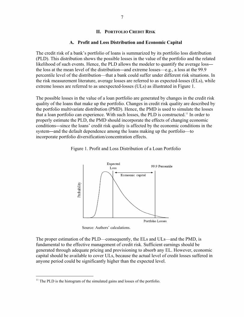
The credit risk of a bank’s portfolio of loans is summarized by its portfolio loss distribution (PLD). This distribution shows the possible losses in the value of the portfolio and the related likelihood of such events. Hence, the PLD allows the modeler to quantify the average loss—the loss at the mean level of the distribution—and extreme losses—e.g., a loss at the 99.9 percentile level of the distribution—that a bank could suffer under different risk situations. In the risk measurement literature, average losses are referred to as expected-losses (ELs), while extreme losses are referred to as unexpected-losses (ULs) as illustrated in Figure 1. The possible losses in the value of a loan portfolio are generated by changes in the credit risk quality of the loans that make up the portfolio. Changes in credit risk quality are described by the portfolio multivariate distribution (PMD). Hence, the PMD is used to simulate the losses that a loan portfolio can experience. With such losses, the PLD is constructed.11 In order to properly estimate the PLD, the PMD should incorporate the effects of changing economic conditions—since the loans’ credit risk quality is affected by the economic conditions in the system—and the default dependence among the loans making up the portfolio—to incorporate portfolio diversification/concentration effects.
Figure 1. Profit and Loss Distribution of a Loan Portfolio
Source: Authors’ calculations. The proper estimation of the PLD—consequently, the ELs and ULs—and the PMD, is fundamental to the effective management of credit risk. Sufficient earnings should be generated through adequate pricing and provisioning to absorb any EL. However, economic capital should be available to cover ULs, because the actual level of credit losses suffered in anyone period could be significantly higher than the expected level.
11 The PLD is the histogram of the simulated gains and losses of the portfolio.

8
The structural approach (SA) is one of the most common approaches to modeling portfolio credit risk, and therefore to estimating PLDs.12 Under the SA, the change in the value of the assets of a borrowing company is related to the change in its credit risk quality.13 The basic premise of this approach is that a borrowing firm’s underlying asset value evolves stochastically over time and default is triggered by a drop in the firm’s asset value below a threshold value, the latter being modeled as a function of the firm’s financial structure. Thus, the likelihood of the firm’s asset value falling below the default-threshold, i.e., defaulting, is summarized by the probability of default (PoD) of the firm (Figure 2).14
Figure 2. The Structural Approach
Source: Authors’ calculations. The distributions behind the stochastic processes driving the firms’ asset values under the SA approach are usually assumed to be parametric.15 For any of these parametric assumptions, 12 Widely known applications of the structural approach include the Credit Metrics framework (Gupton et al, 1997) and the KMV framework (Crosbie and Bohn, 1998).
13 It is assumed that the credit risk quality of a given loan is equivalent to the credit risk quality of the firm requesting the loan. This might not always be the case, since different types of collateral, covenants etc, can make the firm’s and the loan’s credit risk quality differ.
14 The generalization of this approach includes, in addition to the default state, different credit risk quality states (ratings) and thus changes in credit risk quality are also triggered by changes in the firm’s asset value with respect to threshold values.
15 In its most basic version, it is assumed that the firms’ logarithmic asset values are normally distributed (Merton, 1974). The normality assumption has been justified by its simplicity and tractability. From a theoretical point of view, its justification is given by the Central Limit Theorem. However, it has long been observed that market returns exhibit systematic deviations from normality, across virtually all markets. Empirical returns show heavier tails than would be predicted by the normal distribution. Therefore, in most recent versions of the structural approach, alternative parametric distributions have been proposed, including t-distributions, historical simulation, and mixture models. Empirical support for modeling univariate returns with
(continued…)

9
the availability of variables, or proxies, indicating the evolution of the firms’ underlying asset value is of crucial importance for the adequate calibration of the distributions.16
B. Information Restrictions Binding Portfolio Credit Risk Measurement
Although, in recent years, credit risk measurement has been improving rapidly, especially for market-traded instruments, information constraints still impose severe limitations when trying to measure the portfolio credit risk of loans granted to arm’s-length and closely held firms. This is because the approaches that have been developed for the measurement of portfolio credit risk, the SA and the RA, rely on parametric assumptions that, for proper calibration, need data that are nonexistent for these types of firms. It is not possible to observe variables indicating the evolution of the underlying asset value of such firms. Nor, at the portfolio level, is it possible to observe the joint likelihood of credit risk quality changes in the loans making up a portfolio. For arm’s-length and closely held firms, it is usually only possible to observe the default frequencies of loans grouped under different characteristics of the firms (borrowers) to whom the loans have been granted; e.g., economic sector activities or credit-risk quality classes (ratings).17 If the default frequency of a given type of loan is interpreted as the PoD of that type of loan and one assumes that the SA holds, the PoD provides information on one region of the asset value distribution of the firm to whom the loan has been granted; we call this the region of default. The region of default of a specific type of firm can be appreciated in Figure 2 as the region where its asset value (x) is lower than its default threshold (Xd). Accordingly, if the distribution of asset values in Figure 2 is turnaround, the region of default for the firm is defined in Figure 3 as the region where x≥Xd under an assumed distribution. Thus, the PoD of each type of loan in a portfolio represents partial information of the (marginal) asset value distribution of each type of firm to whom the loans of a portfolio have
t-like tails can be found in Danielsson and de Vries (1997) and Hoskin et al (2000). Glasserman et al (2000) present the multivariate modeling framework. Historical simulation for portfolio credit risk is presented by Mina and Xiao (2001) and Butler and Schachter (1998). For mixture models see McLachlan and Basford (1987) and Zangari (1996).
16 The reduced-form approach (RA) represents an alternative to the SA. RA models have been mainly used to model the behavior of credit spreads. This approach treats default as a jump process with exogenous intensity (Duffie and Singleton, 1999). These models rely on variables that are only available for market-traded companies (e.g. bond yield spreads) to calibrate the intensity function for each obligor. A widely known application is the Credit Risk+ framework.
17 For these types of loans, sometimes it is also possible to obtain frequencies of credit risk quality changes. However, for an outsider to the firm (a bank or a regulator) the quality of these statistics at a given point in time is difficult to verify. Therefore, we chose to develop our models assuming the lowest level of data availability.

10
been granted. Using partial information of these marginal distributions, the modelers’ aim is to generate the PMD that describes the joint likelihood of asset value changes of the firms to whom the loans of a portfolio have been granted; equivalently, the PMD that describes the joint likelihood of changes in the credit quality of the loans that make up a portfolio.
Figure 3. The Region of Default
Source: Authors’ calculations.
Undertaking such a task is complicated by the fact that the problem is under-identified. There are infinitely many solutions to such a density and a basis for selecting a particular solution is needed. The traditional route taken is to impose convenient distributional assumptions, representing information that is not available, so that the problem can be analyzed with familiar classical tools. For the specific case of credit risk modeling of arm’s-length and closely held firms, parametric assumptions may not provide an appropriate framework. The lack of adequate data may make it impossible to calibrate the assumed parametric distributions, and these distributions may not be consistent with the analyzed assets’ data-generating processes. If these shortcomings are manifested, erroneous statistical inferences may result and the economic interpretations would be incorrect, undermining banks’ profitability or even threatening their sustainability.
An additional data limitation is that the time series of PoDs are very short, in both developed and developing countries. This lack of adequate data through time represents a significant problem for risk managers who attempt to evaluate the impact of specific macroeconomic and financial events on the credit risk of their respective portfolios. In many models, the number of observations in the time series of PoDs barely exceeds the number of parameters to be estimated. In such situations, although the parameters are determinate, they possess large standard errors, placing a limit on the level of analysis of credit risk through time that can be undertaken by financial institutions.

11
III. PROPOSAL TO IMPROVE PORTFOLIO CREDIT RISK MEASUREMENT
In order to estimate PMDs that incorporate the effects of changing economic conditions, a procedure based on the joint implementation of the CoPoD methodology and the CIMDO methodology has been developed. These methodologies are easily implementable in data constrained environments and improve the measurement of portfolio credit risk. The CoPoD is developed in Segoviano (2006a) and is based on the principle of Maximum Entropy (Jaynes, 1957). The CIMDO is developed in Segoviano (2006b) and is based on applications of the Minimum Cross Entropy approach (Kullback, 1959).18 The CoPoD allows the modeling of PoDs as functions of macroeconomic and financial variables and produces efficient (smaller variance) estimators with few PoD observations. Once the PoDs are modeled, the CIMDO allows inferring PMDs from the estimated PoDs. In comparison to standard portfolio credit risk models, the CIMDO relaxes the reliance on potentially unrealistic statistical assumptions in the measurement of portfolio credit risk. As discussed earlier, this is particularly important for portfolios comprising loans granted to SMEs and non-listed firms. Rather than applying convenient parametric distributional assumptions, representing the information that is not available, the CIMDO defines a selection criterion for choosing one of the infinite number of density specifications that are possible under the under-identified credit risk problem. The CIMDO does not need stock prices, market, or financial variables of individual firms to model the credit risk. Nor is information on the loans’ dependence structure (correlations) needed; it only requires the PoDs of each type of loan making up a portfolio to recover its PMD.
A. The Conditional Probability of Default Methodology
The CoPoD methodology models the empirical frequencies of loan defaults, PoDs, as functions of (identifiable) macroeconomic and financial variables. The detailed development of this methodology is presented in Segoviano (2006a). A summary of the CoPoD is presented in Box 1. PoDs of loans grouped by economic sector (e.g., manufacturing, agriculture, fishing, and tourism) or by risk-rating (e.g., AAA and AA) are usually the only statistic available for modeling the credit risk of SMEs, unlisted and arm’s-length firms. The process of modeling PoDs represents a challenging task, since the time series of PoDs usually contain few observations, thus making OLS estimation imprecise or unfeasible.19
18 A summary of the Maximum and Minimum Cross Entropy approaches is presented in Appendix 1. 19 It is well known that in settings of short time series, OLS estimators possess large variances and can be very sensitive to small changes in the data. These characteristics represent important problems for risk modelers when trying to evaluate the impact of economic shocks in PoDs.

12
Box 1. The Conditional Probability of Default Methodology In this box, a summary of the CoPoD methodology econometric setting is presented. Interested readers in the detailed development may refer to Segoviano (2006a). CoPoD: Rationale Under the Merton (1974) model, a borrower is assumed to default at time T > t, if, at that time, the value of his assets, i
tS , fall below a pre-specified barrier, ita , which is modeled as a function of the borrower's leverage
structure. Therefore, default can be characterized by s(T)≤ ita . Thus, at time t, the PoD at time T is given by
PoDt= ( )i
taΦ , ( 1 )
whereΦ ( ) is the standard normal cumulative distribution function cdf. If we group the PoDs of loans classified under the sectoral activity of the borrower to whom the loans are granted or their risk-rating category in a T-dimensional vector, PoD, each observation in the vector of frequencies of loan defaults PoD represents the empirical measure of PoD for the ith type of borrower at each point in time t. Since each observation in the vector of PoDs is restricted to lie between 0 and 1, we make the following transformation:ai 1−= Φ (PoD), where Φ (.) is the inverse standard normal cdf. We are interested in modeling the PoDs as functions of identifiable macroeconomic and financial developments X, therefore we can formalize the problem as
a X β= + e , ( 2 ) where a is a T-dimensional vector of noisy observations (transformation of the PoDs), X is a known (T x K) matrix of macroeconomic and financial series and β is a K-dimensional vector of unknown coefficients that we are interested in estimating. Consequently, we know X, observe a and wish to determine the unknown and unobservable parameter vector β . CoPoD: Formulation As detailed in Segoviano (2006a), we reformulate the model set in equation (2) as follows. We express our uncertainty aboutβ and e by viewing them as random variables on supports Z and V, respectively; where p(λ ) and w (λ ) represent families of probability density functions for these random variables. Accordingly, the model set in equation (2) can be written in terms of random variables, and the estimation problem is to recover the probability distributions forβ and e; e.g., p(λ ) and w (λ ).
As a result, we treat each kβ as a discrete random variable with a compact support 2≤M< ∞ possible outcomes.
For example if 12, andk kMM z z= represent the plausible extreme values (upper and lower bounds) of kβ .
Therefore, we can express as kβ a convex combination of these two points. That is, there exists [0,1]kp ∈
such that, for 12, (1 )k k k k kMM p z p zβ= = + − . We can do this for each element of β . However, M≥2 may be used to express the parameters in a more general fashion. In this case we also restrict the weights pk to be strictly positive and to sum to 1 for each k. Therefore, we are in a position to rewrite each kβ as a convex
combination of M points. These convex combinations may be expressed in matrix form as β=Zp. We can also reformulate the vector of disturbances, e. Accordingly, we represent our uncertainty about the outcome of the error process by treating each et as a finite and discrete random variable with 2≤J<∞ possible outcomes. We also suppose that there exists a set of error bounds, vt1and vtj, for each et. For example, for J=2, each disturbance may be written as et=wtvt2 + (1-wt) vtJ for [0,1]tw ∈ . However, J≥2 may be used to express the

13
Box 1. The Conditional Probability of Default Methodology (concluded) parameters in a more general fashion. As before, we restrict the weights so as to be strictly positive and to sum to 1 for each t. The T unknown disturbances may be written in matrix form as e=Vw. Using the reparameterized unknowns, β= Zp and e =Vw, we can rewrite the model presented in equation (2) as:
a=XZp+Vw, ( 3 ) This model incorporates the effects of macroeconomic and financial developments into the PoDs at each point in time. It also accounts for possible noise in the data. The information represented by this set of equations is incorporated into the entropy decision rule that is used to recover the distributions p and w. Such information is formulated as a set of moment-consistency constraints that has to be fulfilled by the distributions p and w. The objective of the entropy decision rule is to choose the set of relative frequencies, p and w, that could have been generated in the greatest number of ways consistent with what is known; e.g., the moment-consistency constraints. Thus, following Segoviano (2006a), the probability vectors p and w, are recovered by maximizing the functional:
1 1 1 1
1 1 1 1
1 1 1 1
ln ln
1 1
K M T Jk k t tm m j j
k m t j
T K M Jk k t t
t t tk m m j jt k m j
K M T Jk t
k m j jk m t j
L p p w w
a x z p v w
p T w
λ
θ
= = = =
= = = =
= = = =
⎡ ⎤⎡ ⎤=− − ⎢ ⎥⎢ ⎥⎣ ⎦ ⎣ ⎦⎡ ⎤
+ − −⎢ ⎥⎣ ⎦
⎡ ⎤⎡ ⎤+ − + −⎢ ⎥⎢ ⎥⎣ ⎦ ⎣ ⎦
∑∑ ∑∑
∑ ∑∑ ∑
∑ ∑ ∑ ∑
( 4 )
where Tγ ∈R represents the Lagrange multipliers corresponding to the moment-consistency constraints that
embed the information provided by the data and and Tθ τΚ∈ ∈R R represent the Lagrange multipliers corresponding to the additivity restrictions that are imposed on p and w, since those distributions represent densities; thus, they must add to one. The entropy solution is given by:
1
1 1
ˆexpˆˆ ( )
ˆexp
T kt tk mtk
m M T kt tk mm t
x zp
x z
λλ
λ
=
= =
⎡ ⎤−⎣ ⎦=⎡ ⎤⎡ ⎤−⎢ ⎥⎣ ⎦⎣ ⎦
∑∑ ∑
( 5 )
and by
1
ˆexpˆˆ ( )ˆexp
tt jt
j J tjj
vw
v
λλ
λ=
⎡ ⎤−⎣ ⎦=⎡ ⎤⎡ ⎤−⎣ ⎦⎣ ⎦∑
( 6 )
Once we recover the optimal probability vector p we are in a position to form point estimates of the unknown
parameter vector β as follows β Z p Equally, the optimal probability vector w , may also be used to form point estimates of the unknown disturbance e=V w . Thus, the CoPoD provides a rationale for choosing a particular solution vector p, which is the density that could have been generated in the greatest number of ways consistent with what is known (without imposing arbitrary distributional assumptions). Because we do not want to assert more of the distribution p than is known, we choose the p that is closest to the uniform distribution and also consistent with the available information, expressed as constraints in equation (4). Short time series of PoDs are the norm in most instances. This is because the PoDs of unlisted firms or arm’s-length firms are statistics that are usually recorded with low
14
frequencies (most of the time, annually, quarterly, or monthly). Moreover, PoDs have been recorded from the middle/end of the 1990s in most cases. Although there are exceptions to this norm, even if longer time series exist, it might not be possible to use them if such series belong to economies that have gone through economic structural changes.20 CoPoD improves the measurement of the impact of macroeconomic variables on PoDs and consequently the measurement of loans’ credit risk through time, thereby making a twofold contribution. First, econometrically, it recovers estimators that show greater robustness than OLS estimators in finite sample settings under the mean square error criterion. Second, economically, on the basis of economic theory and empirical evidence, CoPoD incorporates a procedure to select a relevant set of (identifiable) macroeconomic explanatory variables that have an impact on the PoDs. We consider the latter to be a particularly important feature of a model that is to be used in stress testing. This is because if we are interested in making an explicit link between economic shocks and risks and vulnerabilities in financial systems, it is much easier to conduct discussions, negotiations, and make policy recommendations when the results of a risk model can be backed by economic theory and empirical evidence, and when the relevant explanatory variables are identifiable. This approach constitutes a clear improvement over purely statistical or mathematical models that are economically a-theoretical, or models that use underlying nonobservable variables as explanatory variables. CoPoD: Intuition behind efficiency improvements in small sample settings When dealing with time series of PoDs that contain few observations, modeling PoDs as functions of macroeconomic variables represents a challenging task, since OLS estimation becomes imprecise or unfeasible. We have claimed that in these circumstances the CoPoD methodology recovers estimators that show greater robustness than OLS estimators under the MSE criterion. Theoretical proofs, as well as a Monte Carlo experiment, that demonstrate the efficiency gains achieved by CoPoD estimators are presented in Segoviano (2006a). In this section we aim to provide an intuitive explanation of this result. It is well known that for the General Linear Model (GLM), Maximum Likelihood (ML) estimators are equivalent to OLS estimators (under the assumption that the Yi are normally and independently distributed). When ML estimation is computed, first, implicitly, equal weights to each sample observation are assigned. Second, the normal distribution is assumed to be the parametric distributional form that represents the stochastic behavior of the Yi. Then, the unknown parameters are solved by maximizing the probability of observing the Yi, e.g., by maximizing the Yi likelihood function. In order to provide structure to these ideas, we present the analysis developed in Box 2.
20 Common proxies for PoDs are nonperforming loans (NPLs) ratios. Short time series of NPLs are usually common; thus, the CoPoD can be applied exactly in the same way to model NPLs.

15Box 2. Conditional Probability of Default Efficiency
This box presents a heuristic explanation of the robustness of the CoPoD estimators in small sample settings. However, this is intended to be an intuitive exposition. The large and small sample properties of the CoPoD estimators and a Monte Carlo experiment that proves their robustness are presented in Segoviano (2006a). In Appendix 1, we present the Kullback (1959) minimum cross entropy approach (MXED) to recover densities. The MXED objective is to minimize the cross entropy distance between the posterior p distribution and the
prior q distribution. The cross-entropy objective function is defined as [ , ] lnK
kk k
k k
pC p q pkq
⎡ ⎤= ⎢ ⎥
⎣ ⎦∑ . Note that
the MXED can be interpreted as the expectation of a log-likelihood ratio. This interpretation is useful to illustrate the efficiency gains provided by the CoPoD estimation framework. Let 1θ and 2θ be two alternative values of the parameter vector defining two alternative discrete probability distribution characterizations
1( ; )f y θ and 2( ; )f y θ for the distribution of y. The MXED information in 1( ; )f y θ relative to 2( ; )f y θ is given by:
11 2 1
2
( ; )[ ( ; ) , ( ; )] ln ( ; )( ; )y
f yC f y f y f yf y
θθ θ θθ
⎡ ⎤⎡ ⎤= ⎢ ⎥⎢ ⎥
⎣ ⎦⎣ ⎦∑ ( 7 )
1
1
2
( ; )ln( ; )
L yL yθ
θθ
⎡ ⎤⎡ ⎤=Ε ⎢ ⎥⎢ ⎥
⎣ ⎦⎣ ⎦,
where E1[]θ
denotes an expectation taken with respect to the distribution 1( ; )f y θ . It is clear that the MXED
functional in equation (7) can be interpreted as a mean log-likelihood ratio, where averaging is done using weights provided by the distribution 1( ; )f y θ .
If 1 1
2 2
( ; ) ( ; )ln ln( ; ) ( ; )
f y L yf y L y
θ θθ θ
⎡ ⎤ ⎡ ⎤=⎢ ⎥ ⎢ ⎥
⎣ ⎦ ⎣ ⎦ is interpreted as the information in the data outcome y in favor of the
hypothesis 1θ relative to 2θ , then equation (7) can be interpreted as the mean information provided by sample
data in favor of 1θ relative to 2θ under the assumption that 1( ; )f y θ is actually true.
Now, consider the MXED criterion when the distribution 2( ; )f y θ is some discrete distribution p(y) having
discrete and finite support y∈Γ and the distribution 1( ; )f y θ is 1n− ∀ y ∈Γ . In this context, the MXED is given by:
1
1
11[ 1, ] ln
( )
n
i i
nC n pn p y
−
=
⎡ ⎤⎡ ⎤⎢ ⎥⎢ ⎥
= ⎢ ⎥⎢ ⎥⎢ ⎥⎢ ⎥⎢ ⎥⎣ ⎦⎣ ⎦
∑ ( 8 )
1
1ln ( ) ln( )
n
ii
n p n−
=
=− −∑ , ( 9 )
where 1 represents a (nx1) vector of ones so that '1 1 11 ,...,n n n− − −⎡ ⎤= ⎣ ⎦ denotes a discrete uniform distribution,
n is the number of elements in ,Γ p 1 2( , ,..., )np p p= ’ and pi ≡ p(yi). It is evident that minimizing equation (8) is equivalent to maximizing the scaled (by n-1) function ln(pi) in equation (9), equivalently, maximizing the likelihood function in equation (9).

16 Box 2. Conditional Probability of Default Efficiency (concluded)
If we reverse the roles of the distributions the MXED function is defined as:
1
1[ , 1] ln 1
ni
ii
pC p n p
n
−
=
⎡ ⎤⎡ ⎤⎢ ⎥⎢ ⎥
= ⎢ ⎥⎢ ⎥⎢ ⎥⎢ ⎥⎢ ⎥⎣ ⎦⎣ ⎦
∑ (10)
1
ln( ) ln( )n
i ii
p p n=
= +∑ ,
where p = (p1, p2, , pn)’ denotes probability weights on the sample observations. Thus minimizing equation
(10) is equivalent to maximizing 1
ln[ ]n
i ii
p p=
−∑ , which is precisely Shannon’s (1948) entropy measure,
defined in equation (17). Thus, the difference between minimizing equation (8) and equation (10) lies in the calibration of the mean information provided by sample data. In the former case, 1[ 1, ]C n p− , averaging is performed with respect to predata weights n-1for each Yi. Then assuming the uniform distribution to be true, the mean information is interpreted in the context of the expected information in favor of the uniform distribution relative to the postdata estimated probability distribution p. Equivalently, we choose the distribution p(y) that minimizes mean information in favor of the empirical distribution weights, n-1(e.g., assuming that weights n-1 are actually true). This interpretation is consistent with the idea of drawing the distribution p(y) as closely as possible to the uniform distribution, which will concomitantly minimize the expected log-likelihood ratio. Note that this is what we implicitly do when computing ML estimation. From this generic representation, we can see that when we perform standard maximum likelihood estimation, we implicitly give equal weights n-1 to each Yi. Then, given an ex ante fixed (normal) distribution, we choose the distribution’s parameters in a way that the probability of observing the given Yi is as high as possible; e.g., we maximize the likelihood function. In the latter case, 1[ , 1]C p n− e.g., the CoPoD approach, averaging is performed with respect to the postdata probability distribution p; where the p estimates of the probabilities of the Yi, are based on observed data information rather than on fixed predata uniform weights. Assuming that the information contained in the moment-consistency constraints is valid, one would anticipate that the expected log-likelihood ratio is estimated more efficiently in the CoPoD approach because it is calculated with respect to probability weights inferred from data information. Then, assuming the p distribution to be true, the mean information is interpreted in the context of the expected information in favor of the p distribution relative to the predata weights, n-1for each Yi. Equivalently, given an ex ante assumed (fixed) parametric distribution, we adjust its parameters (with information provided by the sample) in such a way that the distribution is maximized. Alternatively, the CoPoD criterion would seem more appealing because: (i) it weights sample observations using different estimates of the probabilities of the Yi, which are based on observed data information rather than on fixed uniform weights and (ii) the distribution of probability weights that is employed is inferred from data information rather than ex ante fixed. Therefore, assuming that the information contained in the moment-consistency constraints is valid, one would anticipate the CoPoD estimators to be more efficient because they are calculated with respect to probability weights inferred from a more efficiently used information base. CoPoD: Selection of explanatory variables The selection of an initial set of macroeconomic variables that are analyzed to determine the significant explanatory variables that define the PoDs’ model specifications is based on an
17
economic hypothesis presented as an integral part of the CoPoD methodology. The initial set of macroeconomic variables is consistent with theoretical arguments and empirical evidence. Economic hypothesis The economic hypothesis that is adopted in the CoPoD methodology implies that fluctuations in key macroeconomic and financial variables have the potential to generate endogenous cycles in credit, economic activity, and asset prices. These cycles, in turn, appear to involve and indeed may amplify financial imbalances, which can place great stress on the financial system. During the upturn of the cycle, banks may increase their lending excessively, in some part, as prices of assets held as collateral increase, and the state of confidence in the system is positive. It is also during this stage that the seeds of financial imbalances are sown and the financial vulnerability (risk) of the economy increases, as do the levels of leverage in the banking system. This hypothesis is consistent with theoretical models with credit constraints and a financial accelerator,21 and theories that emphasize the importance of the incentive structures created under financial liberalization that can exacerbate the intensity of such cycles. The relevant economic theory includes second-generation models in the currency crisis literature, which stress the role of self-fulfilling expectations and herding behavior in determining the intensity of the cycles; models that point out that under financial liberalization the scope for risk-taking is increased; and theories that call attention to the creation of perverse mechanisms, such as moral hazard lending and carry trades, that under financial liberalization can exacerbate banking and currency crises.22 This hypothesis is also consistent with empirical evidence.23 Thus, significant information on systemic vulnerabilities, which have the potential to increase financial risk and thus affect the empirical frequencies of loan defaults experienced by companies in the economy, may be obtained from an analysis of key macroeconomic and financial variables that exhibit regularities when systemic vulnerabilities and macroeconomic imbalances are being created and before they unwind. Equivalently, this hypothesis implies that frequencies of default can be partially explained by lagged values of relevant macroeconomic and financial explanatory variables.24 The initial set of variables that are analyzed is presented in Table 1. 21 See Kiyotaki and Moore (1997).
22 See Obstfeld (1995), Calvo (1998), and Flood and Marion (1999) for the first; see Allen and Gale (1998) for the second; and Dooley (1997) for the third.
23 There is a growing literature documenting this empirical evidence. See Heiskanen (1993), Frankel and Rose (1996), Mishkin (1997), Demirgüc-Kunt and Detragiache (1998), Kaminsky and Reinhart (1999), Kaminsky, Lizondo, and Reinhart (1998), Goldstein, Kaminsky, and Reinhart (2000), Eichengreen and Areta (2000), Reinhart and Tokatlidis (2001), Borio and Lowe (2002), and Goodhart, Hofmann, and Segoviano (2004).
24 Further evidence is presented in Segoviano (2006b). In the latter, the model specifications that were consistent with economic theory, empirical evidence and that showed the best goodness of fit, contained explanatory variables that were lagged values of macroeconomic and financial variables.

18
Table 1. Conditional Probability of Default: Initial Set of Variables
Code Variable Source
HOUP House price index National sources as per detailed documentation and BIS calculations based on national data
SHAPRI Share price index IMF International Financial Statistics
AGGASPRI Aggregate asset price index National sources as per detailed documentation and BIS calculations based on national data
FXDU Nominal foreign exchange IMF International Financial Statistics
REER Real foreign exchange IMF International Financial Statistics
RESER International reserves IMF International Financial Statistics
AVGR Money market interest rate IMF International Financial Statistics
UNEM Unemployment IMF International Financial Statistics
OILP Oil price National sources
MTGR Mortgage bond interest rate National sources
GDP Real GDP IMF International Financial Statistics and OECD
CRE Real aggregate credit (private sector) IMF International Financial Statistics and OECD
CON Consumption aggregate IMF International Financial Statistics
CA Current account balance IMF International Financial Statistics
FDI Foreign direct investment IMF International Financial Statistics
INVE Investment aggregate IMF International Financial Statistics
CON Real consumption Authors’ calculations based on national data
CREOVGDP Ratio of aggregate credit in the financial system to GDP Authors’ calculations based on national data
INVOVGDP Ratio of investment to GDP Authors’ calculations based on national data
CONOVGDP Ratio of consumption to GDP Authors’ calculations based on national data
RECUAOVREINV Ratio of real current account to real investment Authors’ calculations based on national data
M2OVRES Ratio of M2 to international reserves Authors’ calculations based on national data
Difference of long minus LOMISH
Short interest rates Authors’ calculations based on national data
INREVO Realized volatility of money market rates Authors’ calculations based on national data
19
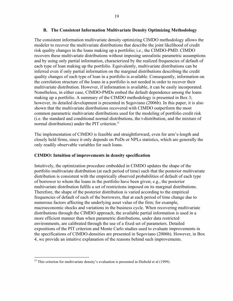
B. The Consistent Information Multivariate Density Optimizing Methodology
The consistent information multivariate density optimizing CIMDO methodology allows the modeler to recover the multivariate distributions that describe the joint likelihood of credit risk quality changes in the loans making up a portfolio; i.e., the CIMDO-PMD. CIMDO recovers these multivariate distributions without imposing unrealistic parametric assumptions and by using only partial information, characterized by the realized frequencies of default of each type of loan making up the portfolio. Equivalently, multivariate distributions can be inferred even if only partial information on the marginal distributions describing the credit quality changes of each type of loan in a portfolio is available. Consequently, information on the correlation structure of the loans in a portfolio is not needed in order to recover their multivariate distribution. However, if information is available, it can be easily incorporated. Nonetheless, in either case, CIMDO-PMDs embed the default dependence among the loans making up a portfolio. A summary of the CIMDO methodology is presented in Box 3; however, its detailed development is presented in Segoviano (2006b). In this paper, it is also shown that the multivariate distributions recovered with CIMDO outperform the most common parametric multivariate distributions used for the modeling of portfolio credit risk (i.e. the standard and conditional normal distributions, the t-distribution, and the mixture of normal distributions) under the PIT criterion.25 The implementation of CIMDO is feasible and straightforward, even for arm’s-length and closely held firms, since it only depends on PoDs or NPLs statistics, which are generally the only readily observable variables for such loans. CIMDO: Intuition of improvements in density specification Intuitively, the optimization procedure embedded in CIMDO updates the shape of the portfolio multivariate distribution (at each period of time) such that the posterior multivariate distribution is consistent with the empirically observed probabilities of default of each type of borrower to whom the loans in the portfolio have been given; e.g., the posterior multivariate distribution fulfils a set of restrictions imposed on its marginal distributions. Therefore, the shape of the posterior distribution is varied according to the empirical frequencies of default of each of the borrowers, that at each period of time change due to numerous factors affecting the underlying asset value of the firm; for example, macroeconomic shocks and variations in the business cycle. When recovering multivariate distributions through the CIMDO approach, the available partial information is used in a more efficient manner than when parametric distributions, under data restricted environments, are calibrated through the use of a fixed set of parameters. Detailed expositions of the PIT criterion and Monte Carlo studies used to evaluate improvements in the specifications of CIMDO-densities are presented in Segoviano (2006b). However, in Box 4, we provide an intuitive explanation of the reasons behind such improvements.
25 This criterion for multivariate density’s evaluation is presented in Diebold et al (1999).
20
Box 3: The Consistent Information Multivariate Density Methodology The detailed formulation of CIMDO is presented in Segoviano (2006b). CIMDO is based on the Kullback (1959) minimum cross-entropy approach (MXED) presented in Appendix 1. For illustration purposes, we focus on a portfolio containing loans given to two different classes of borrowers, whose logarithmic returns are characterized by the random variables x and y, where x,y ∈ɭ i s.t. i=1,..,M.
Therefore, the objective function can now be defined as C[p,q]=∫ ∫p(x,y)ln ( , )( , )
p x yq x y
⎡ ⎤⎢ ⎥⎣ ⎦
dxdy, where q(x,y) the
prior distribution and p(x,y) the posterior distribution ∈ 2R . It is important to point out that the initial hypothesis is taken in accordance with economic intuition (default is triggered by a drop in the firm’s asset value below a threshold value) and with theoretical models (SA) but not necessarily with empirical observations. Thus, the information provided by the frequencies of default of each type of loan making up the portfolio is of prime importance for the recovery of the posterior distribution. In order to incorporate this information into the recovered posterior density, we formulate moment- consistency constraint equations of the form
( ) ( ), ,( , ) , ( , )x y
d d
x yt tx x
p x y dxdy PoD p x y dydx PoDχ χ∞ ∞
= =∫ ∫ ∫ ∫
where ( , )p x y is the posterior multivariate distribution that represents the unknown to be solved. xtPoD and
ytPoD are the empirically observed probabilities of default (PoDs) for each borrower in the portfolio
and ( ) ( ), ,,x y
d dx xχ χ
∞ ∞ are the indicating functions defined with the default thresholds (Figure 3) for each borrower
in the portfolio. In order to ensure that ( , )p x y represents a valid density, the conditions that, ( , )p x y ≥0 and the probability additivity constraint, ∫∫ ( , )p x y dxdy=1, also need to be satisfied. Imposing these constraints on the optimization problem guarantees that the posterior multivariate distribution contains marginal densities that in the region of default, as defined in Figure 3, are equalized to each of the borrowers’ empirically observed probabilities of default. The CIMDO density is recovered by minimizing the functional
[ ], ( , ) ln ( , ) ( , ) ln ( , )L p q p x y p x y dxdy p x y q x y dxdy= −∫ ∫ ∫ ∫ (11)
1 [ , )( , ) x
d
xtx
p x y dxdy PoDλ χ∞
⎡ ⎤+ −⎢ ⎥⎣ ⎦∫ ∫
2 [ , )( , ) y
d
ytx
p x y dydx PoDλ χ∞
⎡ ⎤+ −⎢ ⎥⎣ ⎦∫ ∫
( , ) 1p x y dxdyµ ⎡ ⎤+ −⎣ ⎦∫ ∫
Where 1 2λ λ represent the Lagrange multipliers of the moment-consistency constraints and represents the Lagrange multiplier of the probability additivity constraint. By using the calculus of variations, the optimization procedure is performed. The optimal solution is represented by the following posterior multivariate density as
{ }1 2[ , ) [ , )ˆ ˆˆ ˆ( , ) ( , ) exp 1 ( ) ( )x y
d dx xp x y q x y µ λ χ λ χ
∞ ∞⎡ ⎤= − + + +⎣ ⎦ (12)

21
Box 4: Consistent Information Multivariate Density Optimizing Methodology: Improvements in Density Specification
Analyzing the functional defined in equation (11), it is clear that the consistent multivariate density optimizing methodology recovers the distribution that minimizes the probabilistic divergence; i.e. “entropy distance,” from the prior distribution and that is consistent with the information embedded in the moment-consistency constraints. Thus, out of all the distributions satisfying the moment-consistency constraints, the proposed procedure provides a rationale by which we select the posterior that is closest to the prior, thereby solving the under-identified problem that was faced when trying to determine the unknown multivariate distribution from the partial information provided by the PoDs. The intuition behind this optimization procedure can be understood by analyzing the development of the cross entropy formulation (MXED) in Appendix 1. The MXED objective function presented in equation (20) is an extension of the pure-entropy function in equation (17), which is a monotonic transformation of the multiplicity factor shown in equation (16). The multiplicity factor indicates the number of ways that a particular set of frequencies can be realized (i.e. this set of frequencies corresponds to the frequencies of occurrence attached to specific values of a random variable, Shannon, 1948). Therefore, when maximizing the entropy function subject to a set of constraints, we obtain the set of frequencies (frequency distribution) that can be realized in the greatest number of ways and that is consistent with the constraints (Jaynes, 1957). However, if an initial hypothesis of the process driving the behavior of the stochastic variable can be expressed in the form of a prior distribution, now, in contrast to the maximum entropy pure inverse problem, the problem can be reformulated to minimize the probabilistic divergence between the posterior and the prior. Out of all the distributions of probabilities satisfying the constraints, the solution is the posterior closest to the prior (Kullback, 1959). Although a prior distribution is based on economic intuition and theoretical models, it is usually inconsistent with empirical observations. Thus, using the cross-entropy solution, one solves this inconsistency, reconciling it in the best possible way by recovering the distribution that is closest to the prior but consistent with empirical observations. When we use CIMDO to solve for p(x,y), the problem is converted from one of deductive mathematics to one of inference involving an optimization procedure; e.g., instead of assuming parametric probabilities to characterize information contained in the data, this approach uses the data information to infer values for the unknown probability density. Thus the recovered probability values can be interpreted as inverse probabilities. Using this procedure, we look to make the best possible predictions from the scarce information that we have. This feature of the methodology not only makes implementation simple and straightforward, it also seems to reduce model and parameter risks of the recovered distribution, as indicated by the PIT criterion (Segoviano, 2006b). This is because in order to recover the posterior density, only variables that are directly observable for the type of loans that are the subject of our interest are needed and by construction, the recovered posterior is consistent with the empirically observed probabilities of default. Thus, the proposed methodology represents a more flexible approach to modeling multivariate densities, making use of the limited available information in a more efficient manner.

22
IV. PROPOSED PROCEDURE FOR STRESS TESTING
The proposed stress test procedure involves four steps (Figure 4). (i) The definition of macroeconomic scenarios. These should be extreme but plausible and should be thought to capture the main risks to an economy. The macroeconomic scenarios are usually defined by the mission and the authorities. (ii) The incorporation of macroeconomic shocks into the PoDs of the loans making up the portfolios. The effects of the macroeconomic shocks implied by the previously defined scenarios are incorporated into the probabilities of default of loans grouped by sector or rating. For this purpose, the CoPoD econometric framework is used; thus obtaining CoPoD-PoDs. (iii) The modeling of the portfolios multivariate densities (PMDs). With the use of the CIMDO methodology and the CoPoD-PoDs (as exogenous variables) we recover the PMDs, i.e., the CIMDO-PMDs. (iv) The simulation of portfolios loss distributions (PLDs) and the estimation of their economic capital (EC). The CIMDO-PMD of each bank in the system is used to simulate the possible losses/gains that a bank’s loan portfolio can experience, given its characteristics, e.g., the type of loans held in the portfolio. The losses/gains obtained from this simulation are used to construct the PLD of the portfolio. From this distribution, the EC that a bank should put aside can be determined. This procedure is repeated under each of the macroeconomic scenarios defined in step (i) in order to estimate the EC that a bank should hold—given the riskiness of its portfolio— under different macroeconomic scenarios. The stress testing framework employed allows explicit linkage of macroeconomic shocks to estimation of EC and therefore the evaluation of the banks’ vulnerability under different shocks. It ensures the economic consistency of the estimated risk measurements. We consider these features to be extremely relevant in stress test exercises. This is because if we are interested in making an explicit link from economic shocks to risks and vulnerabilities in financial systems, it is much easier to conduct discussions, negotiations, and make policy recommendations when the results of a risk model can be supported by economic theory and empirical evidence and when the relevant explanatory variables are identifiable. This is a more relevant and practical approach compared with purely statistical or mathematical models that are economically a-theoretical.

23
Figu
re 4
. Stre
ss T
est P
roce
dure
Sim
ulat
ion
Stre
ssed
Ec
onom
ic C
apita
l (V
aR)
Mac
ro
Mod
el
(Aut
horit
ies)
CoP
oD-P
oDs
(Stre
ssed
PoD
s)C
oPoD
CIM
DO
-PM
D
(Stre
ssed
PM
D)
C
IMD
O
-4-2
02
4
-4-2
0
240
0.0
5
0.1
0.1
5
0.2
Mac
ro
Sce
nario
s St
ress
ed
Mac
ro
Varia
bles
Step
1
Step
3
Step
2
Stre
ssed
PLD
Step
4
24
V. STRESS TESTING: EMPIRICAL IMPLEMENTATION IN DENMARK
A. Definition of Macroeconomic Scenarios
On the basis of the current macroeconomic situation and vulnerabilities in the Danish economy, extreme but plausible single factor shocks and macroeconomic scenarios were defined. In all cases, the sizes of the shocks draw from historic information, taking into account a time frame large enough to cover at least an entire economic cycle, or encompassing episodes of financial distress. Economic outlook and vulnerabilities The Danish economy has performed strongly in recent years, and 2005 was no exception. Sound macroeconomic policies, adequate regulatory environments, and flexible labor markets underpin this performance, although temporary factors such as revenue from oil exports and shipping services have further reinforced the positive outcome. After 2000, GDP growth has increased noticeably, reaching 3.0 percent, and continues to expand more rapidly than its potential rate. The unemployment rate has fallen below 4.8 percent, a historical low. Private consumption, exports, and investment are all expanding, and consumer confidence is at its highest level for several years. At the same time, inflation remains low although there are signs that the labor market is becoming increasingly tight, but asset inflation is high. With the economy approaching capacity limits, the immediate challenge is to avoid overheating in the economy. An accommodative monetary policy and rising house prices are two underlying factors that represent a challenge for the authorities (Figure 5). Each provides an added stimulus to private consumption and the overall economy. Monetary policy, however, is constrained because Denmark operates a strict fixed exchange rate link to the euro—which has served Denmark well—so monetary policy is de facto set by the European Central Bank. House prices have grown strongly and added about half a percentage to consumption growth each year via wealth effects and mortgage equity withdrawal. Experience from other small open economies shows that an overheating scenario can then set in very quickly. The recent experience of the Netherlands is one example (OECD, 2006) that could hold some important lessons for Denmark. Therefore, as stated above during discussion of the economic hypothesis, special attention should be given to preventing fluctuations in key macroeconomic and financial variables from becoming endogenous cycles, which have the potential to develop and amplify financial imbalances; thus, placing stress on the financial system.

25
Figure 5. Recent Economic and Financial Developments in Denmark
0
2
4
6
8
10
12
Jan-98 Jan-00 Jan-02 Jan-04 Jan-06
Nominal MCI
Real MCI
Monetary Conditions are accomodative.
0
2
4
6
8
Jan-00 Jul-01 Jan-03 Jul-04 Jan-06
(in percent)
Short-term interest rates follow euro area ...
Denmark
Euro area
0
2
4
6
8
Jan-00 Jul-01 Jan-03 Jul-04 Jan-06
(in percent)
... while long-term ones have fallen lower.
Denmark
Euro area
0
3
6
9
12
15
Jan-00 Jul-01 Jan-03 Jul-04 Jan-06
(12-month change, in percent)
Credit has expanded rapidly ...
Denmark
Euro area
100
150
200
250
300
350
400
96Q1 97Q3 99Q1 00Q3 02Q1 03Q3 05Q1
(Jan 1996 = 100)
... while both shares ...
Stock market indexOMXC20
100
125
150
175
200
225
250
96Q1 99Q1 02Q1 05Q1
(Jan 1996 = 100)
and real estate prices have accelerated.
Nominal House Price Index
Sources: Danmarks Nationalbank; and International Financial Statistics. Recent economic and financial developments in the Danish economy suggest the emergence of risks that could undermine financial stability. Over the last year, the rate of house price increases has been particularly strong, with prices rising at double-digit rates, reaching over 21 percent in the fourth quarter of 2005, the largest increase in nearly 20 years. On the other hand, credit growth has been boosted in parallel, reaching over 20 percent in 2005.
26
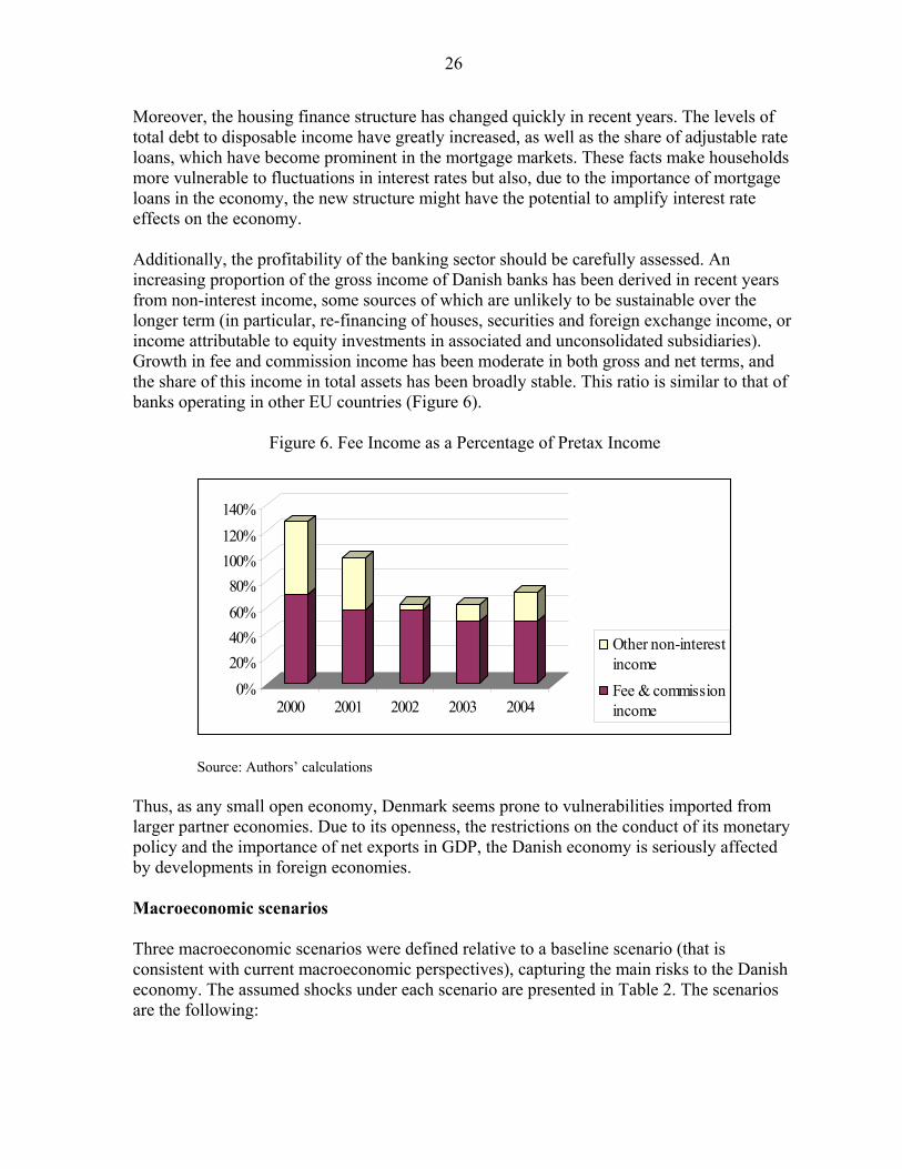
Moreover, the housing finance structure has changed quickly in recent years. The levels of total debt to disposable income have greatly increased, as well as the share of adjustable rate loans, which have become prominent in the mortgage markets. These facts make households more vulnerable to fluctuations in interest rates but also, due to the importance of mortgage loans in the economy, the new structure might have the potential to amplify interest rate effects on the economy. Additionally, the profitability of the banking sector should be carefully assessed. An increasing proportion of the gross income of Danish banks has been derived in recent years from non-interest income, some sources of which are unlikely to be sustainable over the longer term (in particular, re-financing of houses, securities and foreign exchange income, or income attributable to equity investments in associated and unconsolidated subsidiaries). Growth in fee and commission income has been moderate in both gross and net terms, and the share of this income in total assets has been broadly stable. This ratio is similar to that of banks operating in other EU countries (Figure 6).
Figure 6. Fee Income as a Percentage of Pretax Income
0%20%40%60%80%
100%120%140%
2000 2001 2002 2003 2004
Other non-interestincomeFee & commissionincome
Source: Authors’ calculations Thus, as any small open economy, Denmark seems prone to vulnerabilities imported from larger partner economies. Due to its openness, the restrictions on the conduct of its monetary policy and the importance of net exports in GDP, the Danish economy is seriously affected by developments in foreign economies. Macroeconomic scenarios Three macroeconomic scenarios were defined relative to a baseline scenario (that is consistent with current macroeconomic perspectives), capturing the main risks to the Danish economy. The assumed shocks under each scenario are presented in Table 2. The scenarios are the following:

27
Scenario 1: Boom-bust in real estate prices and credit A low interest rate environment has increased the value of collateralizable assets (stocks and real estate). As the borrowing capacity of borrowers depends on the value of their collateralizable assets, higher asset values have contributed to higher lending, which in turn has further fueled economic activity and asset prices. The increased value of assets has increased wealth and thus boosted consumption. Higher consumption has increased aggregate demand and decreased unemployment, with further knock-on effects on asset prices, competitiveness, and economic activity. In this way, the levels of indebtedness in the economy have increased quickly. Eventually, decreases in asset returns—resulting from the sharp increase in asset prices and high levels of indebtedness in the economy—can make economic agents revise their expectations about asset prices and the boom can turn into a bust. Asset prices then start falling and credit growth decreases, suppressing economic activity. Expectations of wealth decrease, consumption falls, aggregate demand falls, GDP falls, and unemployment increases. Depressed collateral prices, higher unemployment and decreasing GDP have a negative impact on banks’ assets, increasing the proportion of non-performing loans. Scenario 2: Foreign shock due to a correction in U.S. imbalances Investors around the world become nervous of global imbalances and withdraw their assets, looking for a “safe haven” in Europe. This results in a reduction of European net foreign investment (NFI). A downward shift in European NFI reduces the demand for loans and therefore reduces the equilibrium interest rate. The reduced level of NFI in Europe reduces the supply of euros in the market for foreign exchange; therefore, the euro appreciates. The Danish krone, pegged to the euro, appreciates against the U.S. dollar and other currencies as well, leading to a loss of competitiveness and lower demand for Danish goods. The trade balance deteriorates, GDP falls, and unemployment rises in Denmark. There is a shift in expectations, negatively affecting private consumption and depressing economic activity further. These effects have a negative impact on banks’ non-performing loans, increasing banks’ losses. Scenario 3: Boom-bust in real estate prices and credit plus an increase in European interest rates The background leading up to this scenario is similar to that described in scenario 1 above, i.e., a boom in asset prices and credit. However, in this scenario, we also assume that the continuation of high oil prices increases inflationary pressures in Europe, prompting the European Central Bank to increase interest rates. The Danmarks National Bank (DNB) follows suit and increases the policy interest rate.

28
Tabl
e 2.
Mac
roec
onom
ic S
cena
rios:
Per
cent
age
Dev
iatio
ns fr
om B
asel
ine
B
asel
ine
Scen
ario
1
Scen
ario
2
Scen
ario
3
Var
iabl
e
2006
20
07
2008
20
06
2007
20
08
2006
20
07
2008
20
06
2007
20
08
GD
P %
y/y
2.
4 2.
2 2.
2 -1
.8
-5
-6.8
-1
.4
-3.2
-4
.1
-2.4
-6
.7
-9.2
Une
mpl
oym
ent*
5.
1 5
5 0.
5 2.
2 3.
8 0.
6 2
3.2
0.7
2.9
5.1
Con
sum
ptio
n %
y/y
2.
5 2.
2 2.
2 -2
.8
-6.9
-9
.1
0.4
-0.5
-1
.2
-3.5
-8
.8
-11.
7 H
ouse
pric
e in
dex
% y
/y
7 3
3 -7
.2
-17.
8 -2
7 -0
.6
-2.9
-5
.5
-15.
6 -2
9.8
-41.
9 In
vest
men
t % y
/y
5.9
4 4
-5.7
-1
2.6
-17.
1 -1
.8
-4.9
-7
.7
-8
-19.
5 -2
6.5
Expo
rts %
y/y
4.
6 5.
5 5.
5 -2
.4
-3.4
-3
.1
-5.9
-8
.3
-8.6
-3
.3
-3.8
-3
.1
Man
ufac
turin
g ou
tput
% y
/y
3.5
3.2
3.2
-3.5
-9
.7
-12.
9 -3
.6
-7.9
-9
.9
-4.6
-1
3 -1
7.5
Con
sum
er p
rice
% y
/y
2.1
1.9
1.9
-0.1
-0
.4
-0.8
-2
-3
.1
-4
0.2
0 -0
.4
Hou
rly w
age
% y
/y
3.7
3.8
3.8
-0.1
-0
.9
-2.7
-0
.3
-1.5
-3
.2
-0.1
-1
.1
-3.5
O
il pr
ice
$/ba
rrel
56
.4
56.4
56
.4
0 0
0 0
0 0
30
30
30
DK
K/U
SD
638
638
638
0 0
0 -2
9 -2
9 -2
9 0
0 0
Mon
ey m
kt in
tere
st ra
te %
poi
nts
3.9
3.9
3.9
0 0
0 0
0 0
2.5
2.5
2.5
Dis
coun
t rat
e %
poi
nts
2.2
2.2
2.2
0 0
0 0
0 0
2.5
2.5
2.5
Shar
e pr
ice
inde
x %
y/y
8
5 5
-0.7
-6
.5
-11.
5 -1
.9
-9.6
-1
4.6
-23.
7 -3
1.6
-30.
8 C
redi
t (pr
ivat
e se
ctor
) % y
/y
8 5
5 -1
,5
-7,0
-1
4,2
0 -1
-2
.7
-1.8
-9
.5
-19.
5
* Pe
rcen
t of l
abor
forc
e na
tiona
l def
initi
on
Th
e sh
ocks
are
repo
rted
as p
erce
ntag
e de
viat
ions
from
the
base
line
scen
ario
(BLS
); th
us, n
eed
to b
e in
terp
rete
d w
ith c
autio
n. F
or e
xam
ple,
a sh
ock
to G
DP
in 2
008
unde
r Sce
nario
3 is
equ
al to
-9.2
per
cent
from
the
BSL
in 2
008.
How
ever
, thi
s sho
ck c
orre
spon
ds to
-2.4
per
cent
from
the
BSL
leve
l in
2005
. Thi
s re
sult
is e
qual
to th
e ac
cum
ulat
ed p
erce
ntag
e in
crea
se in
GD
P un
der t
he B
SL fr
om 2
005
to 2
008
(6.8
per
cent
) min
us th
e pe
rcen
tage
dev
iatio
n fr
om th
e B
SL
in 2
008
(-9.
2 pe
rcen
t).

29
The reassessment of asset values is reinforced by higher interest rates and higher debt servicing, making the boom turn into a bust. As in scenario 1, but only more so, asset prices start falling, consumption decreases, aggregate demand contracts, GDP falls, credit growth decreases, and unemployment increases. Higher interest rates, depressed collateral prices, higher unemployment, and decreasing GDP have a negative impact on banks’ assets and non-performing loans.
B. Necessary Data for Models’ Implementation
In this exercise, we had access to two data sets. In one data set, the loan books of the five largest banks were aggregated by economic sectors.26 For each of these sectors, we had annual observations of nonperforming loan ratios (NPLs)27 from 1991 to 2004 (14 observations) and the percentage loan exposure to each economic sector. The second data set comprised information of loans grouped by risk-rating classifications (RRs).28 For each of these RRs, we had annual observations of empirical frequencies of default29 from 1996 to 2003 (8 observations) and the percentage loan exposures to each RR category. Both variables, NPLs and frequencies of default, appeared to be adequate proxies for PoDs. Therefore, initially, we developed our analysis using both data sets. However, since we were interested on capturing in the best possible way the effects of the business cycle (and therefore, macroeconomic shocks), we decided to base our estimations on the variable that comprised the longest time series. Thus, all the results that are reported from now on in this section are derived using NPLs as proxies for PoDs. Note that the time series that was available and used was very small in statistical terms (14 observations). Note also that information of the dependence structure (correlations) of the borrowers’ PoDs was nonexistent and stock prices or any other market risk indicator of the borrowers was unknown. This certainly represents a highly restricted data set that would make impossible the proper calibration of standard credit risk models.30 However, this data set was enough to properly implement the CoPoD and CIMDO (Table 3).
26 The economic sectors were: public sector, agriculture, fisheries, manufacturing, building, trade, transport, finance and insurance, property administration and households.
27 The NPLs were defined as the nonperforming loan exposure in a given sector over the total loan exposure in the sector.
28 The RRs are based on the DNB failure-rate model described in the DNB Financial Stability Report (2005).
29 The empirical frequencies of default were defined as the number of loans that went into default in a given RR over the total number of loans in the RR category.
30 In Segoviano (2006b), we discuss in detail the data requirements that are necessary for the proper calibration of standard credit risk models.
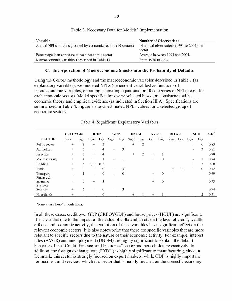
30
Table 3. Necessary Data for Models’ Implementation
Variable Number of Observations Annual NPLs of loans grouped by economic sectors (10 sectors)
14 annual observations (1991 to 2004) per sector
Percentage loan exposure to each economic sector Average between 1991 and 2004. Macroeconomic variables (described in Table 1) From 1970 to 2004.
C. Incorporation of Macroeconomic Shocks into the Probability of Defaults
Using the CoPoD methodology and the macroeconomic variables described in Table 1 (as explanatory variables), we modeled NPLs (dependent variables) as functions of macroeconomic variables, obtaining estimating equations for 10 categories of NPLs (e.g., for each economic sector). Model specifications were selected based on consistency with economic theory and empirical evidence (as indicated in Section III.A). Specifications are summarized in Table 4. Figure 7 shows estimated NPLs values for a selected group of economic sectors.
Table 4. Significant Explanatory Variables
CREOVGDP HOUP GDP UNEM AVGR MTGR FXDU A-R2
SECTOR Sign Lag Sign Lag Sign Lag Sign Lag Sign Lag Sign Lag Sign Lag Public sector + 3 + 2 + 2 - 0 0.83 Agriculture + 5 + 4 - 3 - 3 0.81 Fisheries + 5 + 4 + 2 + 1 0.78 Manufacturing + 4 + 1 - 1 + 0 - 2 0.74 Building + 5 - , + 0, 5 - 3 0.68 Trade + 4 - 0 - 3 + 0 - 0 0.72 Transport - 1 - 0 - 0 + 0 0.69 Finance & insurance - 0 + 3 + 0 0.73 Business Services + 6 - 0 - 3 0.74 Households + 4 - 0 + 1 + 1 - 2 0.71
Source: Authors’ calculations. In all these cases, credit over GDP (CREOVGDP) and house prices (HOUP) are significant. It is clear that due to the impact of the value of collateral assets on the level of credit, wealth effects, and economic activity, the evolution of these variables has a significant effect on the relevant economic sectors. It is also noteworthy that there are specific variables that are more relevant to specific sectors due to the nature of their economic activity. For example, interest rates (AVGR) and unemployment (UNEM) are highly significant to explain the default behavior of the “Credit, Finance, and Insurance” sector and households, respectively. In addition, the foreign exchange rate (FXDU) is highly significant to manufacturing, since in Denmark, this sector is strongly focused on export markets, while GDP is highly important for business and services, which is a sector that is mainly focused on the domestic economy.
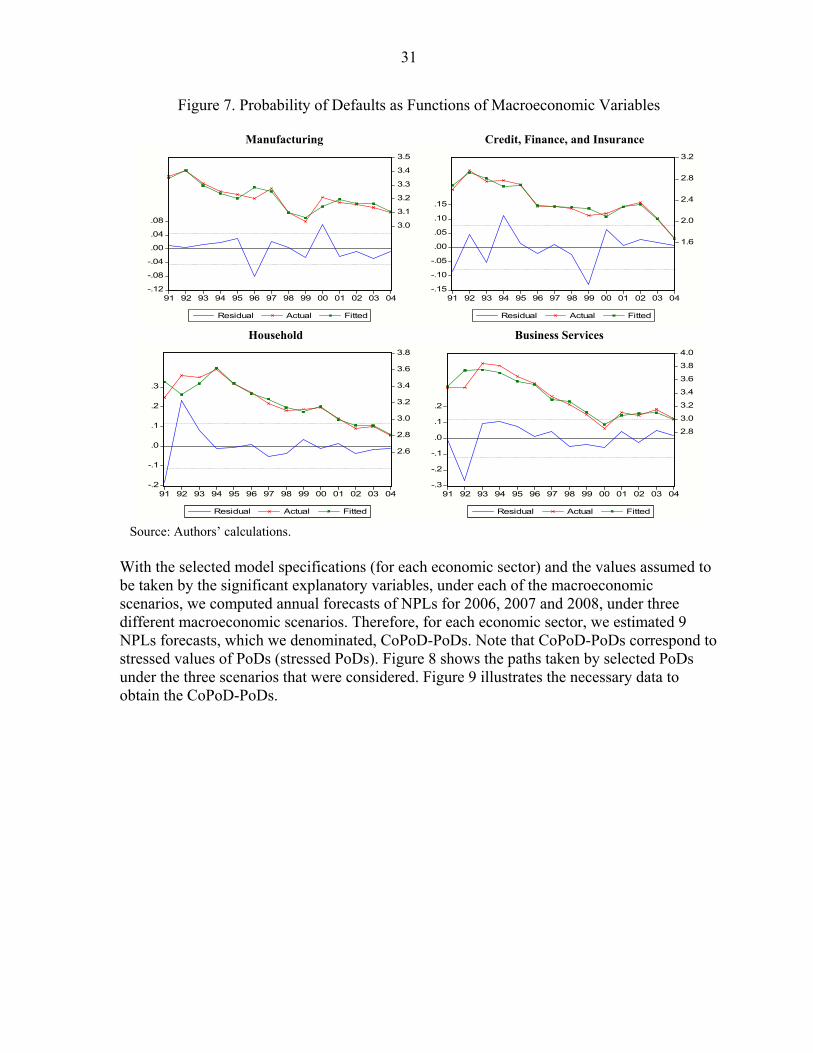
31
Figure 7. Probability of Defaults as Functions of Macroeconomic Variables
Manufacturing Credit, Finance, and Insurance
Household Business Services
Source: Authors’ calculations. With the selected model specifications (for each economic sector) and the values assumed to be taken by the significant explanatory variables, under each of the macroeconomic scenarios, we computed annual forecasts of NPLs for 2006, 2007 and 2008, under three different macroeconomic scenarios. Therefore, for each economic sector, we estimated 9 NPLs forecasts, which we denominated, CoPoD-PoDs. Note that CoPoD-PoDs correspond to stressed values of PoDs (stressed PoDs). Figure 8 shows the paths taken by selected PoDs under the three scenarios that were considered. Figure 9 illustrates the necessary data to obtain the CoPoD-PoDs.
-.3
-.2
-.1
.0
.1
.2
2.8
3.0
3.2
3.4
3.6
3.8
4.0
91 92 93 94 95 96 97 98 99 00 01 02 03 04
Residual Actual Fitted
-.2
-.1
.0
.1
.2
.3
2.6
2.8
3.0
3.2
3.4
3.6
3.8
91 92 93 94 95 96 97 98 99 00 01 02 03 04
Residual Actual Fitted
-.15
-.10
-.05
.00
.05
.10
.15
1.6
2.0
2.4
2.8
3.2
91 92 93 94 95 96 97 98 99 00 01 02 03 04
Residual Actual Fitted
-.12
-.08
-.04
.00
.04
.08 3.0
3.1
3.2
3.3
3.4
3.5
91 92 93 94 95 96 97 98 99 00 01 02 03 04
Residual Actual Fitted
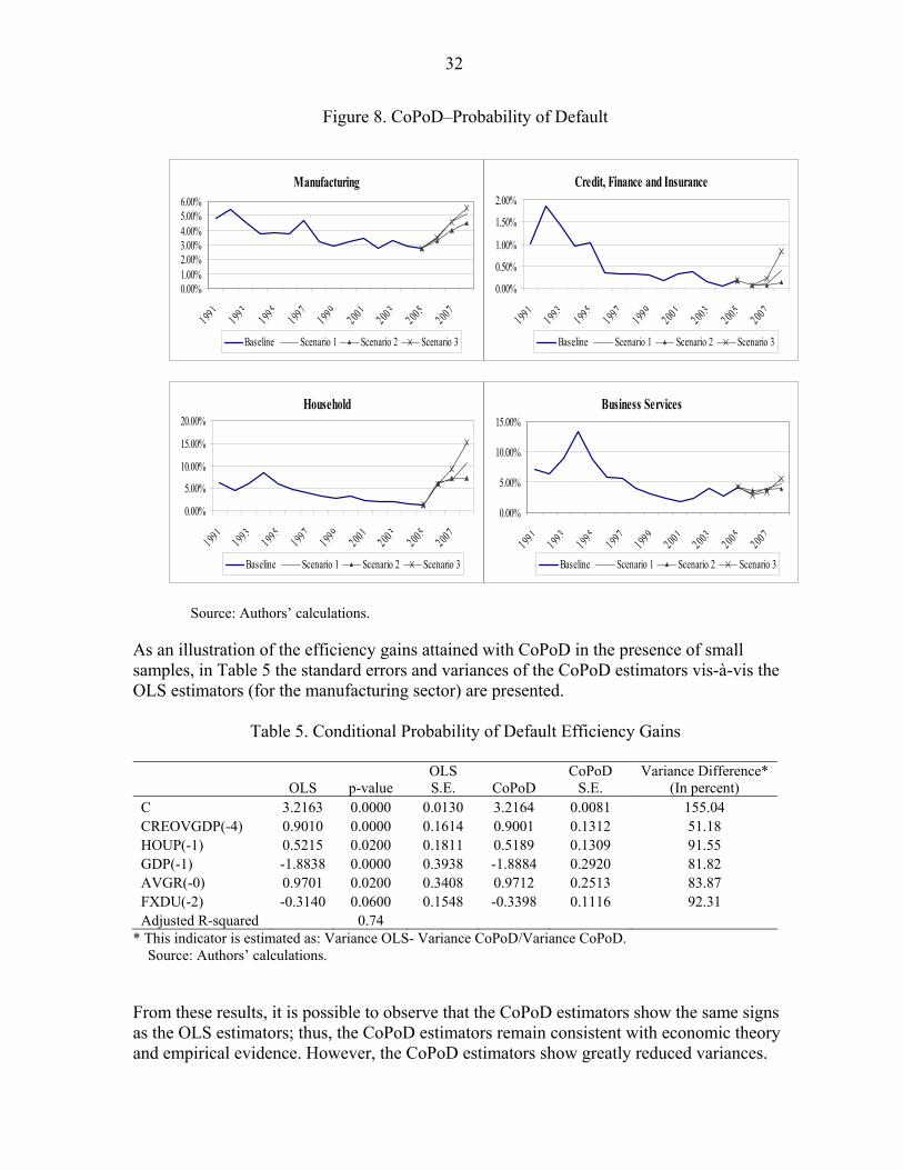
32
Figure 8. CoPoD–Probability of Default
Source: Authors’ calculations.
As an illustration of the efficiency gains attained with CoPoD in the presence of small samples, in Table 5 the standard errors and variances of the CoPoD estimators vis-à-vis the OLS estimators (for the manufacturing sector) are presented.
Table 5. Conditional Probability of Default Efficiency Gains
OLS p-value OLS S.E. CoPoD
CoPoD S.E.
Variance Difference* (In percent)
C 3.2163 0.0000 0.0130 3.2164 0.0081 155.04 CREOVGDP(-4) 0.9010 0.0000 0.1614 0.9001 0.1312 51.18 HOUP(-1) 0.5215 0.0200 0.1811 0.5189 0.1309 91.55 GDP(-1) -1.8838 0.0000 0.3938 -1.8884 0.2920 81.82 AVGR(-0) 0.9701 0.0200 0.3408 0.9712 0.2513 83.87 FXDU(-2) -0.3140 0.0600 0.1548 -0.3398 0.1116 92.31 Adjusted R-squared 0.74
* This indicator is estimated as: Variance OLS- Variance CoPoD/Variance CoPoD. Source: Authors’ calculations.
From these results, it is possible to observe that the CoPoD estimators show the same signs as the OLS estimators; thus, the CoPoD estimators remain consistent with economic theory and empirical evidence. However, the CoPoD estimators show greatly reduced variances.
Manufacturing
0.00%1.00%2.00%3.00%4.00%5.00%6.00%
19911993
19951997
19992001
20032005
2007
Baseline Scenario 1 Scenario 2 Scenario 3
Credit, Finance and Insurance
0.00%
0.50%
1.00%
1.50%
2.00%
19911993
19951997
19992001
20032005
2007
Baseline Scenario 1 Scenario 2 Scenario 3
Household
0.00%
5.00%
10.00%
15.00%
20.00%
19911993
19951997
19992001
20032005
2007
Baseline Scenario 1 Scenario 2 Scenario 3
Business Services
0.00%
5.00%
10.00%
15.00%
19911993
19951997
19992001
20032005
2007
Baseline Scenario 1 Scenario 2 Scenario 3

33
Figure 9. Necessary Data to Incorporate Macroeconomic Shocks into PoDs and PMDs
Subscripts denote time period; e.g., t1,...t14 and forecasts; e.g., f1,..f3. Superscripts denote economic sector; e.g., s1 and s10 correspond to the public and household sectors respectively.
D. Modeling of the Portfolio Multivariate Density
The CIMDO recovers PMDs period by period. It requires PoDs of each type of loan comprising the loan portfolio at each period of time. Therefore, in order to recover PMDs for 2006, 2007 and 2008, under each of the three scenarios, we used the estimated CoPoD-PoDs of each economic sector. The recovered PMDs describe the joint likelihood of changes in the credit risk quality of the loans that make up banks’ portfolios. As indicated in Box 3, the CIMDO-PMD is recovered by minimizing a function of the form described in equation (11). For example, with the 2007 CoPoD-PoDs (stressed PoDs) of each economic sector under scenario 3 (Table 6), moment-consistency constrains were formulated as indicated in Box 3. Consequently, the CIMDO multivariate density in 2007 under scenario 3, corresponding to the analyzed portfolio was recovered by minimizing the following functional:
L[p,q] = ∫..∫p(x1,..,x10) ln p(x1,..,x10) dx1, ..,dx10 -∫..∫ p(x1,..,x10) ln q(x1, .., x10) dx1, .., dx10 ( 13 )
Public sector + ( ) 11 1 10 1 10[ , ).. ,.., ,.., .0055x
dxp x x dx dxλ χ
∞⎡ ⎤−⎢ ⎥⎣ ⎦∫ ∫
Agriculture + ( )2[ , )
2 1 10 1 10.. ,.., ,.., .0490xxd
p x x dx dxλ χ∞
⎡ ⎤−⎢ ⎥⎣ ⎦∫ ∫
Fisheries + ( )3[ , )
3 1 10 1 10.. ,.., ,.., .1059xxd
p x x dx dxλ χ∞
⎡ ⎤−⎢ ⎥⎣ ⎦∫ ∫
Manufacturing + ( )4[ , )
4 1 10 1 10.. ,.., ,.., .0351xxd
p x x dx dxλ χ∞
⎡ ⎤−⎢ ⎥⎣ ⎦∫ ∫
Building + ( ) 55 1 10 1 10[ , ).. ,.., ,.., .0516
xdx
p x x dx dxλ χ∞
⎡ ⎤−⎢ ⎥⎣ ⎦∫ ∫
34
Trade + ( ) 66 1 10 1 10[ , ).. ,.., ,.., .0495x
dxp x x dx dxλ χ
∞⎡ ⎤−⎢ ⎥⎣ ⎦∫ ∫
Transport + ( ) 77 1 10 1 10[ , ).. ,.., ,.., .0287x
dxp x x dx dxλ χ
∞⎡ ⎤−⎢ ⎥⎣ ⎦∫ ∫
Finance + ( ) 88 1 10 1 10[ , ).. ,.., ,.., .0006x
dxp x x dx dxλ χ
∞⎡ ⎤−⎢ ⎥⎣ ⎦∫ ∫
Property + ( )9[ , )
9 1 10 1 10.. ,.., ,.., .0282xxd
p x x dx dxλ χ∞
⎡ ⎤−⎢ ⎥⎣ ⎦∫ ∫
Household + ( )10[ , )
10 1 10 1 10.. ,.., ,.., .0582xxd
p x x dx dxλ χ∞
⎡ ⎤−⎢ ⎥⎣ ⎦∫ ∫
( )1 10 1 10,.., ,.., 1p x x dx dxµ ⎡ ⎤+ −⎣ ⎦∫ ∫
where, 1 10,..,λ λ represent the Lagrange multipliers of the moment-consistency constraints and represents the Lagrange multiplier of the probability additivity constraint.31 The optimal solution is represented by a posterior multivariate density of the form:
{ }1 101 10 1 10 1 2[ , ) [ , )ˆ ˆˆ ˆ( ,.., ) ( ,.., ) exp 1 ( ) ... ( )x x
d dx xp x x q x x µ λ χ λ χ
∞ ∞⎡ ⎤= − + + + +⎣ ⎦ (14 )
Table 6. CoPoD–Probability of Defaults in 2007: Scenario 3
Sector 2007 Public sector 0.0055 Agriculture 0.0490 Fisheries 0.1059 Manufacturing 0.0351 Building 0.0516 Trade 0.0495 Transport 0.0287 Finance & insurance 0.0006 Property administration 0.0282 Households 0.0582
Source: Authors’ calculations.
E. Simulation of Portfolio Loss Distribution and Estimation of Economic Capital
The expected losses (ELs) of the analyzed portfolio under each scenario were estimated. ELs are defined as: EL = PoD x Exposure x Loss Given Default. For this purpose, CoPoD-PoDs (stressed PoDs) for each economic sector, under each scenario, were used. Information on LGDs was not available. As a result, the Basel II guidelines were followed by setting this 31 Like all optimization problems, the Lagrange multipliers reflect the change in the objective function’s value as a result of a marginal change in the constraint set.
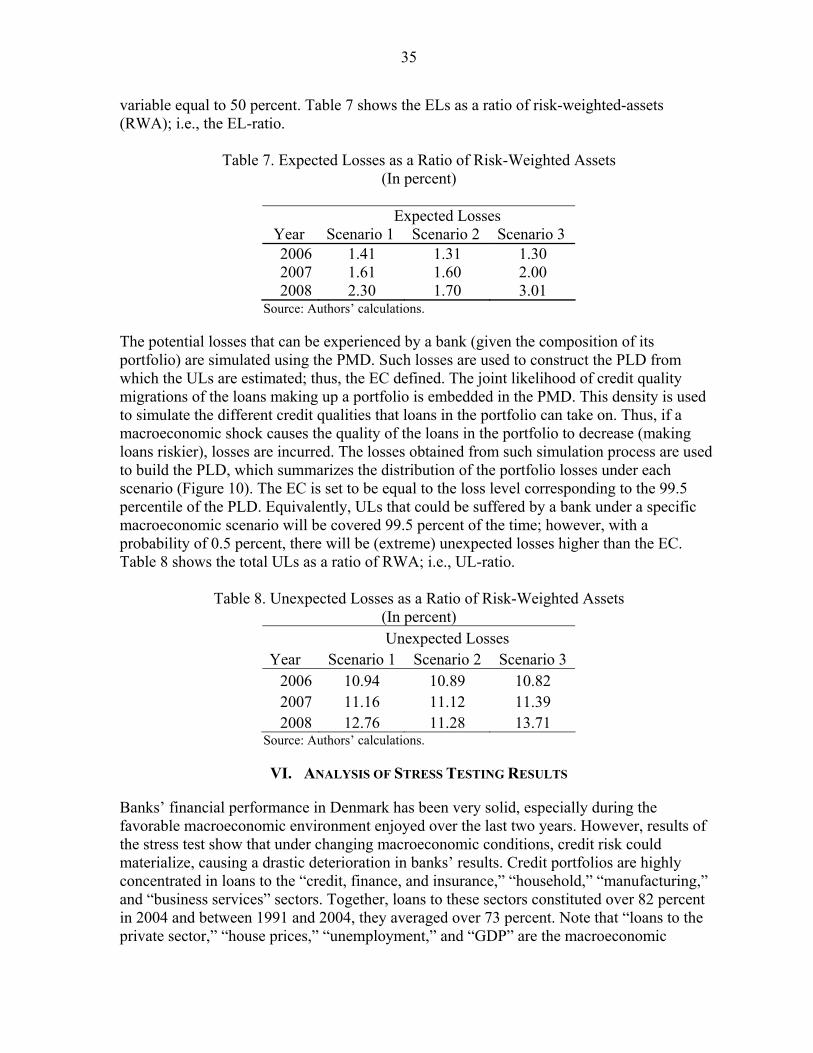
35
variable equal to 50 percent. Table 7 shows the ELs as a ratio of risk-weighted-assets (RWA); i.e., the EL-ratio.
Table 7. Expected Losses as a Ratio of Risk-Weighted Assets (In percent)
Expected Losses Year Scenario 1 Scenario 2 Scenario 3
2006 1.41 1.31 1.30 2007 1.61 1.60 2.00 2008 2.30 1.70 3.01
Source: Authors’ calculations.
The potential losses that can be experienced by a bank (given the composition of its portfolio) are simulated using the PMD. Such losses are used to construct the PLD from which the ULs are estimated; thus, the EC defined. The joint likelihood of credit quality migrations of the loans making up a portfolio is embedded in the PMD. This density is used to simulate the different credit qualities that loans in the portfolio can take on. Thus, if a macroeconomic shock causes the quality of the loans in the portfolio to decrease (making loans riskier), losses are incurred. The losses obtained from such simulation process are used to build the PLD, which summarizes the distribution of the portfolio losses under each scenario (Figure 10). The EC is set to be equal to the loss level corresponding to the 99.5 percentile of the PLD. Equivalently, ULs that could be suffered by a bank under a specific macroeconomic scenario will be covered 99.5 percent of the time; however, with a probability of 0.5 percent, there will be (extreme) unexpected losses higher than the EC. Table 8 shows the total ULs as a ratio of RWA; i.e., UL-ratio.
Table 8. Unexpected Losses as a Ratio of Risk-Weighted Assets (In percent)
Unexpected Losses Year Scenario 1 Scenario 2 Scenario 3
2006 10.94 10.89 10.82 2007 11.16 11.12 11.39 2008 12.76 11.28 13.71
Source: Authors’ calculations.
VI. ANALYSIS OF STRESS TESTING RESULTS
Banks’ financial performance in Denmark has been very solid, especially during the favorable macroeconomic environment enjoyed over the last two years. However, results of the stress test show that under changing macroeconomic conditions, credit risk could materialize, causing a drastic deterioration in banks’ results. Credit portfolios are highly concentrated in loans to the “credit, finance, and insurance,” “household,” “manufacturing,” and “business services” sectors. Together, loans to these sectors constituted over 82 percent in 2004 and between 1991 and 2004, they averaged over 73 percent. Note that “loans to the private sector,” “house prices,” “unemployment,” and “GDP” are the macroeconomic

36
variables that deteriorate faster under the assumed scenarios (Table 2). Deterioration is especially drastic under scenario 3 (followed by scenarios 1 and 2 respectively). These are also the variables that are significant in explaining the default behavior of the sectors to which the banks are more exposed. These effects are captured in the forecasts of the sectors’ PoDs and passed on to the estimated ELs and ULs (Tables 7 and 8).
Figure 10. Profit and Loss Distribution Under the Three Macroeconomic Scenarios
Unexpected Losses
Losses
Freq
uenc
y
SC3SC2SC1
Source: Authors’ calculations.
A buffer large enough to absorb ELs should be generated through adequate pricing and provisioning. Thus, the expected loss Buffer (EL-buffer) was defined as the ratio of pre-tax income plus provisions to RWA. The capital adequacy ratio (CAR) represents the buffer to cover ULs, since the realized level of credit losses experienced under a specific shock could be significantly higher than the expected level. The EL-buffer and the CAR constitute the banking institutions’ total buffer to withstand losses. Overall, the Danish banking institutions’ total buffer as a ratio of RWA has fallen from 2004, and this trend is likely to continue. The reduction in the total buffer is the result of a fall in accumulated provisions and lower solvency ratios, both in absolute levels and as a ratio of RWA. The new IAS/IFRS accounting standards, effective from January 2005 have had a big impact on the EL-buffer via large reductions in provisions. This is seen in Table 9, where the total buffer and its components are presented. Note that from 2004, pre-tax income increased; however, the increase in pretax income was lower than the decrease in provisions.

37
Table 9. Expected Loss-Buffer and Capital Adequacy Ratio Item 2000 2001 2002 2003 2004 Total provisions + pre-tax income 14,799.00 19,314.00 19,057.00 23,551.00 22,485.00 Total capital (capital adequacy) 110,460.47 117,205.30 122,495.97 125,752.22 126,958.58 Total risk-weighted assets 1,135,287.00 1,141,915.00 1,174,840.00 1,168,680.00 1,243,096.00 In percent El-buffer/risk-weighted assets 1.30 1.69 1.62 2.02 1.81 Capital adequacy ratio 9.73 10.26 10.43 10.76 10.21
Source: Authors’ calculations.
Under the current regulatory guidelines and the Basel II proposal, a minimum CAR of 8 percent should always be kept in order to guarantee the regular operations and solvency of a bank. In order to check for this requirement to be fulfilled, we estimated the CAR after the shocks (CAR-S). The decrease that the CAR can suffer after the shocks (CAR-decrease) is defined as the difference between the UL-ratio under each scenario minus the CAR at the end of 2004 (i.e., 10.21 percent). Results are presented in Table 10.
Table 10. CAR-Decrease (In percent)
CAR-decrease Year Scenario 1 Scenario 2 Scenario 3 2006 -0.72 -0.68 -0.61 2007 -0.95 -0.91 -1.17 2008 -2.55 -1.07 -3.50
Source: Authors’ calculations.
The CAR adjusted after the shocks (CAR-S) is estimated as the difference between the CAR at the end of 2004 minus the CAR-decrease. Results are presented in Table 11. From this table we see that the required minimum CAR of 8 percent would be bridged under scenarios 1 and 3 in 2008. In these situations, the solvency of the analyzed banks would be threatened.
Table 11. CAR-S
(In percent) CAR-S
Year Scenario 1 Scenario 2 Scenario 3 2006 9.49 9.54 9.60 2007 9.26 9.31 9.04 2008 7.66 9.14 6.71
Source: Authors’ calculations.
Individual institutions could suffer from much higher losses than those estimated in the stress test. The results presented here represent the results of the “average effect” of the shocks to a group of banks. However, the effects of the shocks are likely to be worse for specific banks.
38
Unfortunately, individual banks’ portfolio credit risk was not able to be assessed due to the use of bank-grouped data. The credit portfolios of other bank groups seem to be riskier, and therefore, the impact of the assumed shocks on those banks’ CAR might probably be higher. The stress test did not include smaller banks; however, the exposure of lending to agriculture and fisheries is the highest among those banks. Some of these banks have grown rapidly. During the challenging times in the late 1980s and early 1990s, it was typically the banks that had grown fastest that also experienced the largest losses. Thus, it is very likely that the potential losses (ELs and ULs) of the assumed shocks might be larger among smaller banks. The effects of shocks to unemployment and interest rates might be larger than they appeared. Lending by banking institutions to households has increased significantly during recent years. In January 2005, the annual growth rate exceeded 20 percent. Growth in this sector has mainly been attributable to the introduction of adjustable-rate bank mortgage loans to homeowners as an alternative to traditional capital-market financing via mortgage-credit institutions. The introduction of mortgage-credit loans with an option to defer amortization has had a significant impact on the composition of loan portfolios. The total debt of households continued to rise at a higher rate than their disposable income; thus, the burden on households has increased. However, low interest rates in recent periods have temporarily neutralized the budget impact of the growing indebtedness. Nonetheless, all these factors will likely make households more vulnerable to fluctuations in interest rates and unemployment. The increase in PoDs, ELs and ULs is consistent across the scenarios (Scenario 3 is the most severe, followed by Scenarios 1 and 2) and over time (the cumulative effects of the macroeconomic shocks over the three-year horizon are reflected in the increasing PoDs, ELs and ULs over the three-year period). These results indicate that credit risk could materialize quickly, if the accelerated and acute increase in house prices and levels of leverage in the economy developed into macroeconomic imbalances, leading to a boom-bust in real estate prices and credit. Moreover, results clearly indicate that current developments in the market, which seem to increase the vulnerability of households to interest rate fluctuations, as well as foreign shocks (as indicated by scenario 3), could reinforce the stress to the banking system. The macroeconomic shocks that were considered (and as a result, the simulated increases in PoDs, ELs, and ULs) may be extreme; but they are plausible. Thus, credit risk clearly remains a major risk factor for the Danish banking system.
VII. CONCLUSIONS
The information requirements (presented in Table 3) necessary for the implementation of the CoPoD and the CIMDO methodologies are less stringent than the information requirements necessary for the proper calibration and implementation of standard credit risk methodologies; therefore their implementation is feasible and straightforward, even under the data constraints that usually bind portfolio credit risk modeling. The CoPoD methodology is designed to recover robust estimators in settings of short time series, incorporating the effects of changing macroeconomic and financial developments into PoDs. The CIMDO methodology recovers portfolio multivariate distributions (PMDs),

39
avoiding reliance on possibly unrealistic statistical assumptions in settings of partial information. CIMDO can be implemented using CoPoD-PoDs; thus, recovering PMDs that also reflect the impact of changing economic conditions. Consequently, if CIMDO-PMDs are used to simulate the profit and loss distributions (PLDs) of bank portfolios and therefore, estimate their economic capital (EC), these EC estimations will embed the effect of changing economic conditions. As a result, the joint implementation of CoPoD and CIMDO provides a useful tool that leads to earlier recognition of banks’ risks as macroeconomic conditions change, making a contribution to the challenging task of portfolio credit risk measurement through time. Moreover, if the joint implementation of the CoPoD and CIMDO methodologies is performed within the framework of stress testing, it becomes possible to quantify the impact of pre-specified macroeconomic shocks on banking systems’ estimates of EC and therefore, quantify the systems’ resilience to specific shocks. Equivalently, this course of action allows us to identify explicit links between economic shocks and risks and vulnerabilities in financial systems. The risk measurements produced by these methodologies are consistent with economic theory and empirical evidence. We consider these features to be extremely relevant in the stress test exercises performed as part of the FSAPs. This is because it is much easier to conduct discussions, negotiations, and make policy recommendations when the results of a risk model can be backed by economic theory and empirical evidence.
40
Appendix 1: Entropy in a Nutshell Given nonexperimental data generation processes (DGP) in economics and finance, and the corresponding data available for applied econometric analysis, economists face the problem of how to make predictions for the population or how to construct an image of it, using the information at hand. Unfortunately, in many cases, the models that economists use for analysis contain unknowns that are unobservable and indeed are not accessible to direct measurement. Consequently, in order to recover the unknown parameters, representing the economic system of interest, economists are faced with an inverse problem that can be formalized as follows. Our interest focuses on the unknown and unobservable frequencies p=(p1, p2,...,pk) that represent the data generating process. However, it is the outcome of an economic variable y, what is observable. Thus, in order to recover p, the indirect measurements on the observable y must be used. Equivalently, from partial information y, we try to define p. In this context, consider the following finite, discrete, linear, problem:
y=Xp (15) where y=(y1, y2,...,yT)’ is a T dimensional vector of observations (data), p is an unobservable K dimensional vector of frequencies and X is a known (T x (K>T)) non invertible matrix. Thus, out of all the probability distributions that satisfy equation (15) and fulfill the
conditions 1kk
p =∑ and pk ≥ 0 we are asked to recover or choose unambiguous probabilities
pk. Given this specification, the information contained in equation (15) does not appear adequate to determine the unknown probabilities p. That is because the number of data points are less than the number of unknowns. In its present form the problem appears under-specified; e.g., the problem is ill-posed, and the basis for assigning a probability is, at this point, unresolved. In these circumstances, creative assumptions are usually employed to induce a well-posed problem that is amenable to solution. However, the imposition of inconsistent assumptions may lead to erroneous interpretations and conclusions. Because usually we must cope with partial-incomplete information and ill-posed inverse problems, we would like to use a principle or formalism that provides us with the “best” conclusions possible based on the data available. In looking for such a principle, or formalism, two requirements appear essential (Jaynes, 1984). We know something but we do not know everything or perhaps not enough to proceed in a traditional way and we do not want to claim any more or any less than we know. These are the guidelines on which the entropy principle is based. The entropy formalism seeks to make the “best” predictions possible from the information that is available and provides a basis for transforming the latter into a distribution of probabilities describing our state of knowledge.

41
Entropy: Modeling foundations The “entropy of the distribution of probabilities” is an axiomatic method used by Shannon (1948) to define a unique function to measure the uncertainty of a collection of events.32 In developing this approach, Shannon (1948) supposed that an experiment with N trials (repetitions) was carried out. This experiment had K possible outcomes (states). He assumed that N1, N2, ....., NK represented the number of times that each outcome occurs in the experiment of length N, where ∑Nk=N, Nk ≥0, and k=1, 2, ..., K. In this setting there are N trials and each trial has K possible outcomes; therefore, there are KN conceivable outcomes in the sequence of N trials. Of these, a particular set of frequencies,
pk= kNN
or Nk = Npk for k= 1,2, ...,K
can be realized in a given number of ways as measured by the multiplicity factor (possible permutations). Thus, the number of ways that a particular set of N_{k} is realized, can be represented by the multinomial coefficient:
W = 1 2
!! !... !k
NNp Np Np
= !!k k
NN∏
or its monotonic function
lnW = lnN! – 1
lnK
kk
N=∑ ! (16)
Shannon (1948) manipulated equation (16), as presented in Segoviano (2006b), to obtain the Shannon (1948) entropy measure, which is defined as
H(p) = -1
K
kk
p=∑ ln kp , (17)
where kp ln kp = 0 for ln kp = 0. Jaynes (1957) proposed to make use of the entropy concept to choose an unknown distribution of probabilities when only partial information is available. He proposed to maximize the function presented in equation (17), subject to the limited available data, in order to obtain the probability vector p that can be realized in the greatest number of ways consistent with the known data.
32 The origins of the entropy concept go back to the XIXth century with the work developed by Boltzman and continued subsequently by Maxwell, Gibbs, Bernoulli and Laplace.

42
The rationale provided by Jaynes (1957) for choosing a particular solution, i.e., probability vector p from partial information, is known as the Principle of Maximum Entropy (MED). Let
L = – K
kk
p∑ ln kp + 1
T
tt
λ=∑ )(
K
t k kk
y p ft x⎡ ⎤−⎢ ⎥⎣ ⎦∑ +µ 1
K
kk
p⎡ ⎤−⎢ ⎥⎣ ⎦∑ , (18)
be the Lagrange function. Then, the problem of maximum entropy is to maximize L. In this function, the information contained in the data has been formalized in 1≤ t ≤T
moment-consistency constraints of the form 1
( )K
k t k tk
p f x y=
=∑ . These moment-consistency-
constraints are formulated with T functions {f1 (x), f2 (x), ...., f T (x)} representing the information contained in the data and with a set of observations (averages or aggregates) {y1(x), y2 (x), ..., yT (x)} that are consistent with the distribution of probabilities {p1, p2,..., pk}.
In this function, the additivity restriction 1
K
kk
p=∑ =1 has to be fulfilled as well, since p
represents a probability distribution. Note also that tλ represents the Lagrange multiplier of each of the 1≤ t ≤T moment-consistency constraints and represents the Lagrange multiplier of the probability additivity constraint. Using the method of Lagrange multipliers, the Maximum Entropy solution is given by:
ˆ kp = ( )
1 1
1
ˆexpK T
t t kk t
f xλ= =
⎡ ⎤−⎢ ⎥⎣ ⎦∑ ∑
exp ( )1
ˆT
t t kt
f xλ=
⎡ ⎤⎢ ⎥⎣ ⎦∑ (19)
An extension to the rationale provided by Jaynes is the minimum cross entropy distribution (MXED) developed by Kullback (1959). Under the MXED, it is assumed that, in addition to the T moment constraints, some form of conceptual knowledge exists about the properties of the system and that this knowledge can be expressed in the form of a prior probability vector q. In contrast to the MED pure inverse problem framework, the objective may be reformulated as being to minimize the cross entropy distance between the posterior p and the prior q. The cross-entropy objective function is defined as follows:
C [ ],k kp q = K
kk
p∑ ln k
k
pq
⎡ ⎤⎢ ⎥⎣ ⎦
(20)
subject to T moment-consistency constraints ( )1
K
k t kk
p f x=∑ and the additivity restriction
1
K
kk
p=∑ .

43
Consequently, the probability vector p may be recovered by minimizing the Lagrangian function:
L =
K
kk
p∑ ln k
k
pq
⎡ ⎤⎢ ⎥⎣ ⎦
+ 1
T
tt
λ=∑ ( )
K
t k t kk
y p f x⎡ ⎤−⎢ ⎥⎣ ⎦∑ +
1K
kk
pµ⎡ ⎤−⎢ ⎥⎣ ⎦∑
(21)
where tλ and µ represent Lagrange multipliers. Using the method of Lagrange multipliers, the optimal solution to the cross-entropy problem is
ˆ kp =
( )1 1
ˆexp
kK T
k t t kk t
q
q f xλ= =
⎡ ⎤⎢ ⎥⎣ ⎦
∑ ∑exp ( )
1
K
t t kt
f xλ=
⎡ ⎤⎢ ⎥⎣ ⎦∑
(22)
Shannon’s entropy measure E (pk), presented in equation (17), can be interpreted as a measure of the degree of uncertainty in the distribution of probabilities, representing the extent to which the distribution is concentrated on specific points as opposed to being dispersed over many points. E (pk) takes its maximum value lnK, when the distribution is maximally dispersed and thus uniformly distributed on the range of the distribution, in other
words, when p1 = p2 = ... = pk = 1K
. E (pk) takes its minimum value 0, when the distribution
is maximally informative in that p degenerates on one particular xk value, in other words, 1kp = and pj = 0, k j∀ ≠
The objective of maximizing E (pk) in the absence of any constraints, other than the
additivity restriction 1
K
kk
p=∑ = 1, can be interpreted as choosing pk to be the maximally
uniform distribution. This is because, as mentioned above, E (pk) takes its maximum value
when p1 = p2 = ... = pk = 1K
.
However, in the presence of T moment constraints, as suggested by Jaynes, the objective can be interpreted as choosing the pk’ s to be as maximally uninformative as the moment constraints allow. This objective is consistent with the goal of not wanting to assert more of the distribution pk, than is known. In other words, irrelevant information is “minimized out.” When, in addition to the T moment constraints, supplementary information in the form of a prior probability is incorporated into the optimization framework, the Kullback cross entropy framework recovers the density that could have been generated in the greatest number of
44
ways consistent with these constraints and that has the smallest entropic distance from the prior distribution. The entropic distance between pk and qk is not a metric distance33 but it does satisfy C ,k kp q⎡ ⎤⎣ ⎦ = 0 for pk = qk and C ,k kp q⎡ ⎤⎣ ⎦ > 0, whenever pk ≠ qk . Note that the definition of
C ,k kp q⎡ ⎤⎣ ⎦ does not contain a negative sign, so cross entropy is minimized rather than maximized. Note also that equation (22) reduces to equation (19) when q(x) is constant, i.e., a uniform distribution indicating no prior information about X.
33 This is because C[p(x),q(x)]≠C[q(x),p(x)], however, for our objective, this property is not particularly important because the prior distribution is taken to be fixed in estimation problems. Our interest centers on choosing the posterior distribution that solves the moment equations and that is as close as possible to the prior distribution.
45
References Allen, F., and D. Gale, 1998, “Bubbles and Crises,” The Economic Journal, Vol. 110. ———, 1999, “Bubbles, Crises, and Policy,” Oxford Review of Economic Policy, Vol. 15,
No. 3, pp. 9–18. Altman, E., A. Elizondo, and Miguel Segoviano, 2002, “Medicion Integral del Riesgo de
Credito,” edited Limusa, Mexico. Basel Committee on Banking Supervision, 1988, “International Convergence of Capital
Measurement and Capital Standards,” Basel, July 1988.
Basel Committee on Banking Supervision, 1988, “New Basel Capital Accord,” Basel, January 2001. Berger, A., and G. Udell, 1990, “Collateral, Loan Quality, and Bank Risk,” Journal of
Monetary Economics, Vol. 25, pp. 21–42. ———, 2003, “The Institutional Memory Hypothesis and the Procyclicality of Bank
Lending Behavior,” Bank for International Settlements Working Paper 125. Bernanke, B., and M. Gertler, 1989, “Agency Costs, Collateral, and Business Fluctuations,”
American Economic Review, Vol. 79, pp. 14–31. ———, and S. Gilchrist, 1998, The Financial Accelerator in a Quantitative Business Cycle
Framework,” NBER Working Paper No. 6455. ———, and S. Gilchrist, 1999, “The Financial Accelerator in a Quantitative Business Cycle
Framework,” in Handbook of Macroeconomics, edited by J.B. Taylor and M. Woodford,Vol. 1C, pp. 1341–93.
Black, F., and M. Scholes, 1973, “The Pricing of Options and Corporate Liabilities,” Journal
of Political Economy, Vol. 81, 637–59. Bank for International Settlements, 1999, “The Monetary and Regulatory Implications of
Changes in the Banking Industry,” Bank for International Settlements Conference Papers No.7.
———, 2001, 71st Annual Report. Borio, C., and W. Fritz, 1995, “The Response of Short-Term Bank Lending Rates to Policy
Rates: A Cross-Country Perspective,” Bank for International Settlements Working Paper No. 27.

46
Borio, C., N. Kennedy, and S. Prowse, 1994, “Exploring Aggregate Asset Price Fluctuations Across Countries: Measurement, Determinants and Monetary Policy Implications,” Bank for International Settlements Economic Paper 40.
Borio, C., and P. Lowe, 2002, “Asset Prices, Financial and Monetary Stability: Exploring the
Nexus,” BIS Working Paper 114. Butler, J., and B. Schachter, 1998, “Estimating Value-at-Risk with a Precision Measure by
Combining Kernel Estimation with Historical Simulation,” Review of Derivatives Research Vol. 1, pp. 371–90.
Calvo, G., 1998, “Varieties of Capital-Market Crises,” edited by G. Calvo and M. King, in
The Debt Burden and its Consequences for Monetary Policy (New York: McMillan Press).
Caprio, G., and D. Klingebiel, 1996, “Bank Insolvency: Cross-Country Experiences,”
(Washington: World Bank).
Cihak, M., 2006, “How Do Central Banks Write on Financial Stability,” IMF Working Paper 06/163, (Washington, International Monetary Fund). Crosbie, P., and J. Bohn, 1998, “Modeling Default Risk,” KMV LLC. Danielsson, J. and C. G. de Vries, 1997, “Tail Index and Quantile Estimation with Very High
Frequency Data,” Journal of Economics and Finance, Vol. 4, pp. 241–57. Demirgüc-Kunt, A., and E. Detriagiache, 1998, “The Determinants of Banking Crises:
Evidence from Developing and Developed Countries,” Staff Papers, International Monetary Fund, Vol. 45, No. 1.
———, 1999, “Financial Liberalization and Financial Fragility,” edited by B. Pleskovic and
J. Stiglitz in Proceedings of the World Bank Annual Conference on Development Economics.
———, 2005, “Cross-Country Empirical Evidence of Systemic Banking Distress: A
Survey,” IMF Working Paper 05/96 (Washington: International Monetary Fund). Diebold, F., T. Gunther, and A. Tay, 1998, “Evaluating Density Forecasts with Applications
to Financial Risk Management,” International Economic Review, Vol. 39, pp. 863– 83.
Diebold, F., J. Hahn, and A. Tay, 1999, “Multivariate Density Forecast Evaluation and
Calibration in Financial Risk Management: High-Frequency Returns on Foreign Exchange,” The Review of Economics and Statistics, Vol. 81(4), pp. 661–73.
Dooley, M., 1997, “A Model of Crises in Emerging Markets,” NBER, Working Paper 6300.

47
Drees, B., and C. Pazarbasioglu, 1998, “The Nordic Banking Crises: Pitfalls in Financial
Liberalization?” IMF Occasional Paper No. 161( Washington: International Monetary Fund).
Duffie, J. D., and K. J. Singleton, 1999, “Modelling Term Structures of Defaultable Bonds,”
Review of Financial Studies Vol. 12, pp. 687–720. Eichengreen, B., and C. Areta, 2000, “Banking Crises in Emerging Markets: Presumptions
and Evidence,” Center for International and Development Economics Research Paper, C00-115.
———, and M. Bordo, 2003, “Crises Now and Then: What Lessons From the Last
Era of Financial Globalization,” Edited by P. Mizen, Chapter 3 in Monetary History, Exchange Rates, and Financial Markets; Essays in honor of Charles Goodhart, Vol. 2, pp. 52–91 (Cheltenham: Edward Elgar).
Flood, R., and N. Marion, 1999, “Perspectives on the Recent Currency Crisis Literature,”
International Journal of Finance and Economics, Vol. 4, 1, pp. 1–26. Frankel, J., and A. Rose, 1996, “Currency Crashes in Emerging Markets: An Empirical
Treatment,” Journal of International Economics, Vol. 41, pp. 351–66. Glasserman, P., P. Heidelberger, and P. Shahabuddin, 2000, “Portfolio Value-at-Risk with
Heavy-Tailed Risk Factors,” Money, Economics, and Finance Working Paper (New York: Columbia Business School, Columbia University.).
Goldstein, M., G. Kaminsky, and C. Reinhart, 2000, “Assessing Financial Vulnerability: An
Early Warning System for Emerging Markets,” Institute for International Economics, Washington DC.
Goodhart, Charles, 1995, “Price Stability and Financial Fragility,” edited by K. Sawamoto,
Z. Nakajima, and H. Taguchi in Financial Stability in a Changing Environment, St. Martin’s Press.
———, and Boris Hofmann, 2003, “Deflation, Credit, and Asset Prices,” in P. Siklos and R. Burdekin, The Anatomy of Deflation, Cambridge University Press. ———, and Miguel Segoviano, 2004, “Bank Regulation and
Macroeconomic Fluctuations,” Oxford Review of Economic Policy, Vol. 20, No. 4, pp. 591–615.
Goodhart, Charles, and Miguel Segoviano, 2004, “Basel and Procyclicality: A Comparison
of the Standardized and IRB Approaches to an Improved Credit Risk Method,” London School of Economics, Financial Markets Group, Discussion Paper 524.

48
Gupton, M., C. Finger, and M. Bhatia, 1997, “Credit Metrics Technical Document,” Morgan Guaranty Trust Company, Risk Management Research.
Heiskanen, R., 1993, “The Banking Crisis in the Nordic Countries,” Kansallis Economic
Review, Vol. 2, pp. 13–19. Hodrick, R., and E. Prescott, 1980, “Post-War U.S. Business Cycles: An Empirical
Investigation,” Discussion Paper 451, Carnegie-Mellon University. Hofmann, B., 2001, “The Determinants of Private Sector Credit in Industrialized Countries:
Do Property Prices Matter?” BIS Working Paper No. 108.
Hoskin, J.R.M., G. Bonti, and D. Siegel, 2000, “Beyond the Lognormal,” Risk, 13, No. 5 (May), pp. 59–62.
Jaynes, E., 1957, “Information Theory and Statistical Mechanics,” Physics Review Vol. 106,
pp. 620–30. _____, 1984, “Prior Information and Ambiguity in Inverse Problems,” Edited by D.W.
McLaughlin in Inverse Problems, pp.151–66, SIAM Proceedings, American Mathematical Society, Providence, Rhode Island.
Judge, G., and A. Golan, 1992, “Recovering Information in the Case of Ill-Posed Inverse
Problems with Noise,” University of California Berkeley. Kaminsky, G., S. Lizondo, and C. Reinhart, 1998, “Leading Indicators of Currency Crises,”
Staff Papers, International Monetary Fund, Vol. 5 (January), pp. 1–48. Kaminsky, G., and C. Reinhart, 1996, “Banking and Balance of Payments Crises: Models
and Evidence,” Board of Governors of the Federal Reserve Working Paper (Washington: Board of Governor of the Federal Reserve).
———,, 1999, “The Twin Crisis: The Causes of Banking and Balance
of Payments Problems,” American Economic Review, Vol. 89, pp. 473–500. Kaminsky, G., and S. Schmukler, 2003, “Short-Run Pain, Long-Run Gain: The Effects of
Financial Liberalization,” NBER Working Paper 9787. Kiyotaki, N., and J. Moore, 1997, “Credit Cycles,” Journal of Political Economy, Vol. 105,
pp. 211–48.
Knight, M., and J. Santaella, 1997, “Economic Determinants of IMF\ Financial Arrangements,” Journal of Development Economics, Vol. 54, pp. 405–36.
Krugman, P., 1979, “A Model of Balance of Payments Crises,” Journal of Money, Credit,
and Banking, Vol. II(3), pp. 311–25.

49
Kullback, J., 1959, Information Theory and Statistics, (New York: John Wiley). Kullback, S., and R. Leibler, 1951, “On Information and Sufficiency,” Annals of
Mathematical Statistics, Vol. 22, 79–86.
McLachlan, G., and K. Basford, 1987, “Mixture Models: Inference and Applications to Clustering, Marcel Dekker,” New York and Basel.
McKinnon, R., and H. Pill, 1996, “Credible Liberalizations and International Capital Flows:
The Over Borrowing Syndrome,” edited by T. Ito and A. Krueger in Financial Deregulation and Integration in East Asia, pp. 7–45 (Chicago: University of Chicago Press).
Merton, R., 1974, “On the Pricing of Corporate Debt: The Risk Structure of Interest Rates,”
The Journal of Finance, Vol. 29, pp. 449–70.
Mina, J., and Y. Xiao, 2001, “Return to RiskMetrics: The Evolution of a Standard,” RiskMetrics.
Minsky, H., 1982, “Can It Happen Again?” in Essays on Instability and Finance, M.E.
Sharpe. Mishkin, F., 1997, “Understanding Financial Crises: A Developing Country Perspective,”
edited by Michael Bruno and Boris Pleskovic in Annual World Bank Conference on Development Economics 1996, Washington, DC, International Bank for Reconstruction and Development, 29-61.
Obstfeld, M., 1995, “Models of Currency Crises with Self-Fulfilling Features,” NBER
Working Paper 5285 (Cambridge, Massachusetts: MIT Press). ———, and K. Rogoff, 1995, “The Mirage of Fixed Exchange Rates,” NBER Working
Paper 5191 (Cambridge, Massachusetts: MIT Press). OECD, 2006, “2006 Economic Review, Denmark,” Economic and Development Review
Committee, (Paris). Pukelsheim, F., 1994, “The Three Sigma Rule,” American Statistician, Vol. 48(4), pp. 88–91. Reinhart, C., and I. Tokatlidis, 2001, “Before and After Financial Liberalization,” University
of Maryland, (unpublished). Saurina, J., and C. Trucharte, 2004, “The Impact of Basel II on Lending to Small and
Medium-Sized Firms: A Regulatory Policy Assessment Based on Spanish Credit Register Data,” Journal of Financial Services Research, Vol. 26:2, pp. 121–144.

50
Segoviano, Miguel, 2004, “A System for Measuring Credit Risk When Only Limited Data is Available,” Credit Risk International, London, October 2004.
———, 2006a, “The Conditional Probability of Default Methodology,” Financial Markets
Group, London School of Economics, Discussion Paper 558. ———, 2006b, “The Consistent Information Multivariate Density Optimizing
Methodology,” Financial Markets Group, London School of Economics, Discussion Paper 557.
Segoviano, Miguel, and P. Lowe, 2002, “Internal Ratings, the Business Cycle and Capital
Requirements: Some Evidence from an Emerging Market Economy,” BIS Working Paper 117, LSE/FMG discussion paper 428.
Shannon, C., 1948, “A Mathematical Theory of Communication,” Bell System, Technical Journal, Vol. 27, pp. 379–423.
Vassalou, M., and Y. Xing, 2002, “Default Risk in Equity Returns,” Columbia University
Working Paper. Zangari, P., 1996, “An Improved Methodology for Measuring VaR,” RiskMetrics Monitor,
2nd Quarter, pp.7–25.