portfolio credit risk - risklab risklab
TRANSCRIPT


TheGoodrich-Rabobankswap:1983
5.5 million (11% fixed) Once a year
(LIBOR – x) % Semiannual
5.5 million Once a year
(LIBOR – y) % Semiannual
11%annualLIBOR+0.5%(Semi)
BelgiandentistsU.S.SavingsBanks
MorganGuaranteeTrust
Rabobank
AAAratedB.F.Goodrich
BBB-rated
Swap Swap

Reviewofbasicconcepts
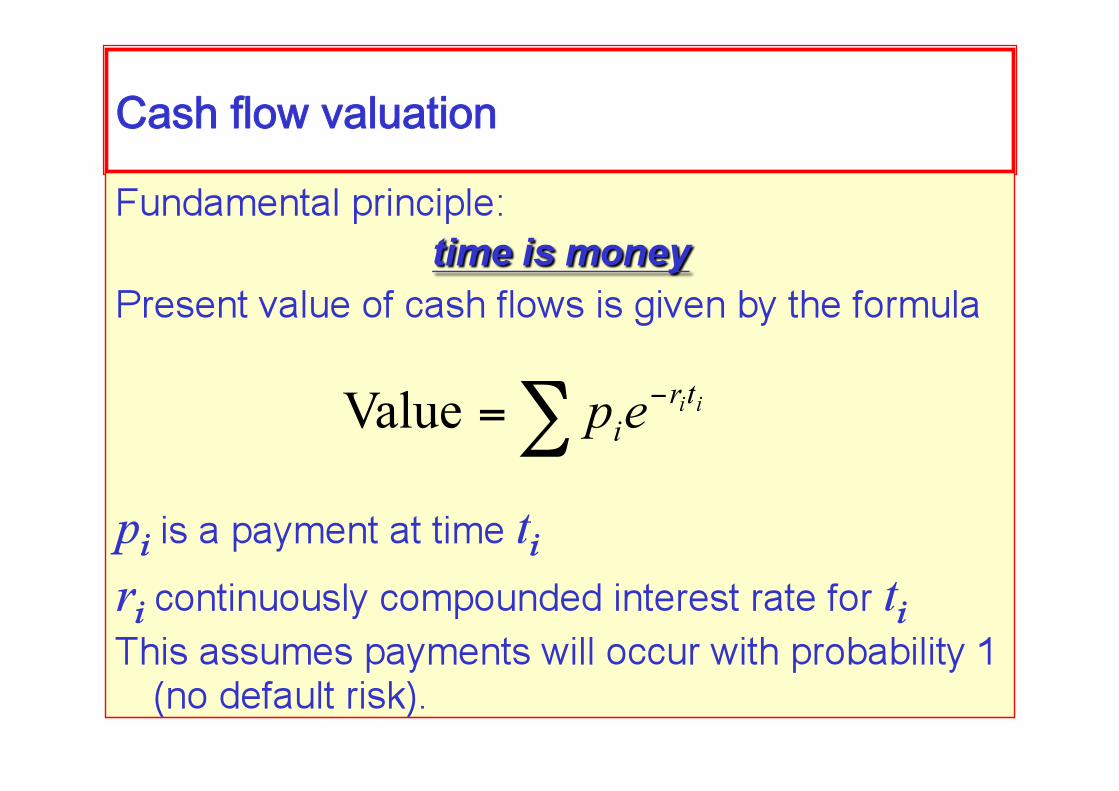
Cashflowvaluation

Creditpremium
The discounted value of cash flows, when there is probability of default, is given by
qi denotes the probability that the counter-party is solvent at time ti
Thelargerthedefaultrisk(qsmall),thesmalleritsvalue.
Thehigherthecreditrisk(qsmall),thehigherthepayments,topreservethesamepresentvalue

Thecreditspread
Since , we can write
the loan is now valued as
Default-prone interest rate increases.

Firstmodel:twocreditstates
What is the credit spread? Assume only 2 possible credit states: solvency and default
Assume the probability of solvency in a fixed period (one year, for example), conditional on solvency at the
beginning of the period, is given by a fixed amount: q
According to this model, we have
which gives rise to a constant credit spread:

ThegeneralMarkovmodel
In other words, when the default process follows a Markov chain,
the credit spread is constant, and equals
Solvency Default
Solvency q 1 - q Default 0 1
Goodrich-Morganswap
The fixed rate loan

G-RBCreditMetricsanalysis:setup
The leg to consider for Credit Risk is the one between JPMorgan and BF Goodrich
Cashflows of the leg (in million USD): 0.125 upfront 5.5 per yr, during 8 years
Assume: constant spread h = 180 bpi 2 state transition probabilities matrix

G-RBCreditMetrics:expectedcashflows
Since Expected[cashflows] = ($cashflows) * Prob{non_default}
Then E[cashflows] = .125 + Sum( 5.5 * P{nondefault @ each year})
But at the same time E[cashflow] =

G-RBCreditMetrics:probabilityofdefault
Under our assumptions: P {non-default} = exp(-h) = exp(-.018) = .98216 constant for each year
The 2 state matrix: BBB D
BBB .9822 .0178
D 0 1

G-RBCreditMetrics:computecashflows
Inputs P{default of BBB corp.} = 1.8%;
1-exp(0.018)=0.9822 The gvmnt zero curve for August 1983 was r = (.08850,.09297,.09656,.0987855,.10550, .104355,.11770,.118676) for years (1,2,3,4,5,6,7,8)
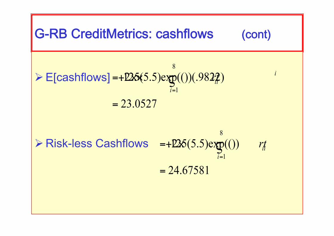
G-RBCreditMetrics:cashflows (cont)
E[cashflows]
Risk-less Cashflows

G-RBCreditMetrics:Expectedlosses
Therefore E[loss] = 1 – ( E[cashflows] / Non-Risk Cashflow) = .065776
i.e. the proportional expected loss is around 6.58% of USD 24.67581 million
Or roughly E[loss] = 1.623 (USD million)

Non-constantspreads
Adefault/no-defaultmodel
(suchasCreditRisk+)
leadstoconstantspreads,unlessprobabilitiesvarywith
time
Inordertofitnon-constantspreads,andbeabletofitthemodeltomarketobservations,oneneedstoassumeeither:
• Time-varyingdefaultprobabilities• Multi-ratingsystems(suchascredit-metrics)
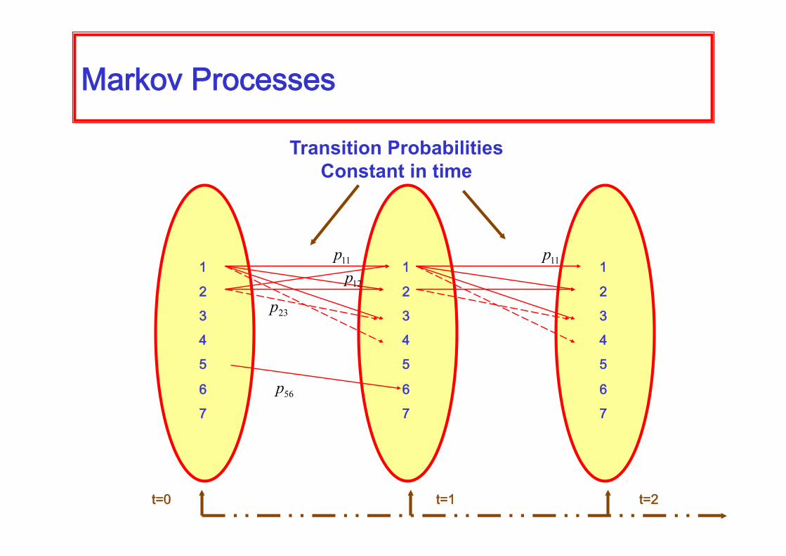
MarkovProcesses
1
2
3
4
5
6
7
1
2
3
4
5
6
7
1
2
3
4
5
6
7
Transition Probabilities Constant in time
t=0 t=1 t=2

Transitionprobabilities
Conditional probabilities, which give rise to a matrix with n credit states,
… … …
:
:
: :
… …
Pij = cond prob of changing from state i to state j

Creditratingagencies
There are corporations whose business is to rate the credit quality of corporations, governments, and also of specific debt issues.
The main ones are: Moody’s Investors Service, Standard & Poor’s, Fitch IBCA, Duff and Phelps Credit Rating Co

StandardandPoor’sMarkovmodel
AAA AA A BBB BB B CCC D
AAA 0.9081 0.0833 0.0068 0.0006 0.0012 0.0000 0.0000 0.0000
AA 0.0070 0.9065 0.0779 0.0064 0.0006 0.0014 0.0002 0.0000
A 0.0009 0.0227 0.9105 0.0552 0.0074 0.0026 0.0001 0.0006
BBB 0.0002 0.0033 0.0595 0.8693 0.0530 0.0117 0.0012 0.0018
BB 0.0003 0.0014 0.0067 0.0773 0.8053 0.0884 0.0100 0.0106
B 0.0000 0.0011 0.0024 0.0043 0.0648 0.8346 0.0407 0.0520
CCC 0.0022 0.0000 0.0022 0.0130 0.0238 0.1124 0.6486 0.1979
D 0 0 0 0 0 0 0 1

Longtermtransitionprobabilities
Transition probability between state i and state j, in two time steps, is given by
In other word, if we denote by A the one-step conditional probability matrix, the two-step transition probability matrix is given by
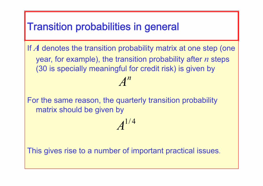
Transitionprobabilitiesingeneral
If A denotes the transition probability matrix at one step (one year, for example), the transition probability after n steps (30 is specially meaningful for credit risk) is given by
For the same reason, the quarterly transition probability matrix should be given by
This gives rise to a number of important practical issues.
CreditLoss

CreditExposure It is the maximum loss that a
portfolio can experience at any time in the future, taken with a certain confidence level.
Evolutionofthemark-to-marketofa20-monthswapExposure(99%)
Exposure(95%)

RecoveryRate–LossGivenDefault
When default occurs, a portion of the value of the portfolio can usually be recovered. Because of this, a recovery rate is always considered when evaluating credit losses. It represents the percentage value which we expect to recover, given default.
Loss-given-default is the percentage we expect to lose when default occurs:
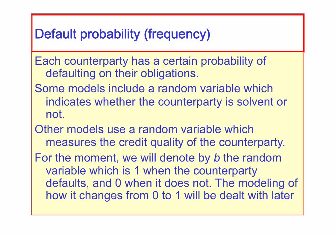
Defaultprobability(frequency)
Each counterparty has a certain probability of defaulting on their obligations.
Some models include a random variable which indicates whether the counterparty is solvent or not.
Other models use a random variable which measures the credit quality of the counterparty.
For the moment, we will denote by b the random variable which is 1 when the counterparty defaults, and 0 when it does not. The modeling of how it changes from 0 to 1 will be dealt with later

Measuringthedistributionofcreditlosses
For an instrument or portfolio with only one counterparty, we define:
Credit Loss = b x Credit Exposure x LGD
Randomvariable:
Dependsonthecreditqualityofthecounterparty
Number:
Dependsonthemarketriskoftheintrumentorportfolio
Number:
Usually,thisnumberisauniversalconstant(55%),butmorerefinedmodelsrelateittothemarketandthecounterparty

Measuringthedistributionofcreditlosses(2)
For a portfolio with several counter-parties, we define:
Credit Loss = (b x Credit Exposure x LGD)
Randomvariable:
Normallydifferentfordifferentcounterparties
Number:
Normallydifferentfordifferentportfolios,samefor
thesameportfolios
Number:
Usually,thisnumberisauniversalconstant(55%),butmorerefinedmodelsrelateittothemarketandthecounterparty
Σ i i i
i

NetReplacementValue
The traditional approach to measuring credit risk is to consider only the net replacement value
NRV = (Credit Exposures)
This is a rough statistic, which measures the amount that would be lost if all counter-parties default at the same time, and at the time when all portfolios are worth most, and with no recovery rate.
Σ i
i
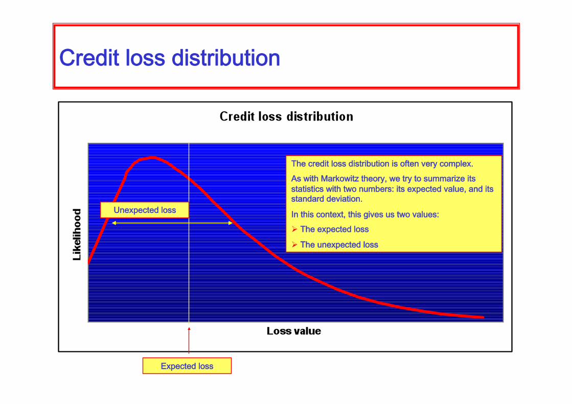
Creditlossdistribution
Expectedloss
Unexpectedloss
Thecreditlossdistributionisoftenverycomplex.
AswithMarkowitztheory,wetrytosummarizeitsstatisticswithtwonumbers:itsexpectedvalue,anditsstandarddeviation.
Inthiscontext,thisgivesustwovalues: Theexpectedloss
Theunexpectedloss

CreditVaR/WorstCreditLoss
Worst Credit Loss represents the credit loss which will not be exceeded with some level of confidence, over a certain time horizon.
A 95%-WCL of $5M on a certain portfolio means that the probability of losing more than $5M in that particular portfolio is exactly 5%.
CVaR represents the credit loss which will not be exceeded in excess of the expected credit loss, with some level of confidence over a certain time horizon:
A daily CVaR of $5M on a certain portfolio, with 95% means that the probability of losing more than the expected loss plus $5M in one day in that particular portfolio is exactly 5%.

Usingcreditriskmeasurementsintrading Marginal contribution to risk When considering a new instrument to be traded as part of a certain
book, one needs to take into account the impact of the new deal in the credit risk profile at the time the deal is considered. An increase of risk exposure should lead to a higher premium or to a deal not being authorized. A decrease in risk exposure could lead to a more competitive price for the deal.
Remuneration of capital Imagine a deal with an Expected Loss of $1M, and an unexpected loss
of $5M. The bank may impose a credit reserve equal to $5M, to make up for potential losses due to default; this capital which is immobilized will require remuneration; because of this, the price of any credit-prone contract should equal
Price = Expected Loss + (portion) Unexpected loss
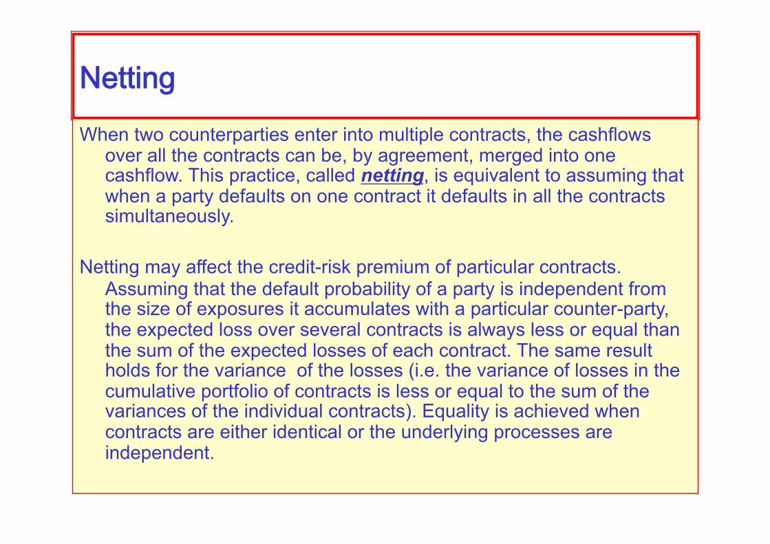
NettingWhen two counterparties enter into multiple contracts, the cashflows
over all the contracts can be, by agreement, merged into one cashflow. This practice, called netting, is equivalent to assuming that when a party defaults on one contract it defaults in all the contracts simultaneously.
Netting may affect the credit-risk premium of particular contracts. Assuming that the default probability of a party is independent from the size of exposures it accumulates with a particular counter-party, the expected loss over several contracts is always less or equal than the sum of the expected losses of each contract. The same result holds for the variance of the losses (i.e. the variance of losses in the cumulative portfolio of contracts is less or equal to the sum of the variances of the individual contracts). Equality is achieved when contracts are either identical or the underlying processes are independent.
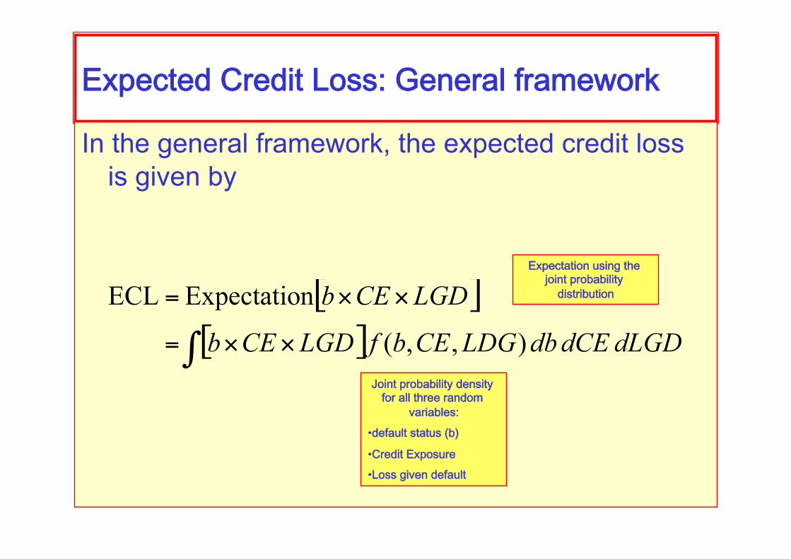
ExpectedCreditLoss:Generalframework
In the general framework, the expected credit loss is given by
Expectationusingthejointprobabilitydistribution
Jointprobabilitydensityforallthreerandom
variables:
• defaultstatus(b)
• CreditExposure• Lossgivendefault
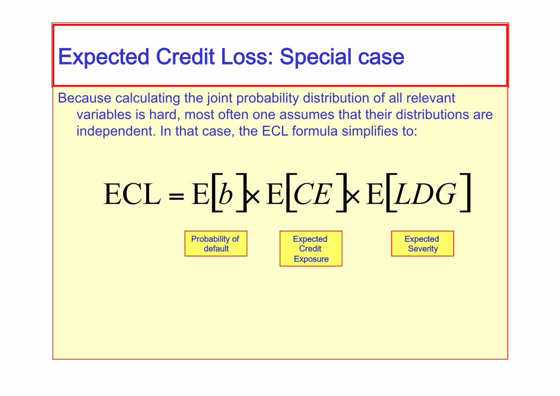
ExpectedCreditLoss:SpecialcaseBecause calculating the joint probability distribution of all relevant
variables is hard, most often one assumes that their distributions are independent. In that case, the ECL formula simplifies to:
Probabilityofdefault
ExpectedCreditExposure
ExpectedSeverity

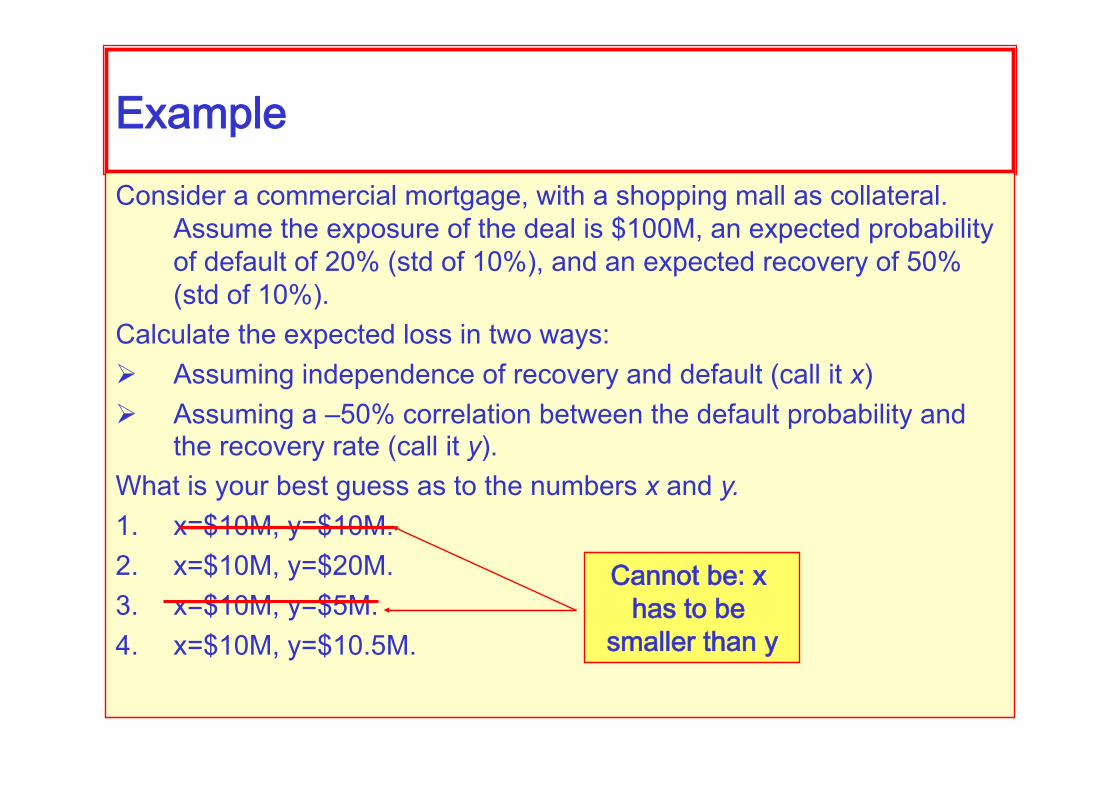
ExampleConsider a commercial mortgage, with a shopping mall as collateral.
Assume the exposure of the deal is $100M, an expected probability of default of 20% (std of 10%), and an expected recovery of 50% (std of 10%).
Calculate the expected loss in two ways: Assuming independence of recovery and default (call it x) Assuming a –50% correlation between the default probability and
the recovery rate (call it y). What is your best guess as to the numbers x and y. 1. x=$10M, y=$10M. 2. x=$10M, y=$20M. 3. x=$10M, y=$5M. 4. x=$10M, y=$10.5M.
Cannotbe:xhastobesmallerthany

Tree-basedmodel
0
1
-1 -1
1
0

Correlatingdefaultandrecovery
Assume two equally likely future credit states, given by default probabilities of 30% and 10%.
Assume two equally likely future recovery rates, given by 60% and 40%.
With a –50% correlation between them, the expected loss is
EL = $100M x (0.375x0.6x0.3 + 0.375x0.4x0.1 + 0.125x0.4x0.3 + 0.125x0.6x0.1) = $100M x (0.0825 + 0.0225) = $10.5M
Probabilitiescalibratedtostatedcorrelations

Goodrich-RabobankExample
Consider the swap between Goodrich and MGT. Assume a total exposure averaging $10M (50% std), a default rate averaging 10% (3% std), fixed recovery (50%).
Calculate the expected loss in two ways Assuming independence of exposure and default (call it
x) Assuming a –50% correlation between the default
probability and the exposure (call it y). What is your best guess as to the numbers x and y. 1. x=$500,000, y=$460,000. 2. x=$500,000, y=$1M. 3. x=$500,000, y=$500,000. 4. x=$500,000, y=$250,000.

Goodrich-RabobankExample
Consider the swap between Goodrich and MGT. Assume a total exposure averaging $10M (50% std), a default rate averaging 10% (3% std), fixed recovery (50%).
Calculate the expected loss in two says Assuming independence of exposure and default (call it
x) Assuming a –50% correlation between the default
probability and the exposure (call it y). What is your best guess as to the numbers x and y. 1. x=$500,000, y=$450,000. 2. x=$500,000, y=$1M. 3. x=$500,000, y=$500,000. 4. x=$500,000, y=$250,000.
Cannotbe:xhastobelarger
thany

Correlatingdefaultandexposure
Assume two equally likely future credit states, given by default probabilities of 13% and 7%.
Assume two equally likely exposures, given by $15M and $5M.
With a –50% correlation between them, the expected loss is
EL = 0.5 x (0.125x$15Mx0.13 + 0.125x$5Mx0.07 + 0.375x$15Mx0.07 + 0.375x$5Mx0.13) = 0.5 x ($0.24M + $0.04 + $0.40M + $0.24M) = $460,000

Example23-2:FRMExam1998Question39
“Calculate the 1 yr expected loss of a $100M portfolio comprising 10 B-rated issuers. Assume that the 1-year probability of default of each issuer is 6% and the recovery rate for each issuer in the event of default is 40%.”

Example23-2:FRMExam1998Question39
“Calculate the 1 yr expected loss of a $100M portfolio comprising 10 B-rated issuers. Assume that the 1-year probability of default of each issuer is 6% and the recovery rate for each issuer in the event of default is 40%.”
0.06 x $100M x 0.6 = $3.6M

Variationofexample23-2.
“Calculate the 1 yr unexpected loss of a $100M portfolio comprising 10 B-rated issuers. Assume that the 1-year probability of default of each issuer is 6% and the recovery rate for each issuer in the event of default is 40%.
Assume, also, that the correlation between the issuers is
1. 100% (i.e., they are all the same issuer) 2. 50% (they are in the same sector) 3. 0% (they are independent, perhaps because
they are in different sectors)”

Solution
1. The loss distribution is a random variable with two states: default (loss of $60M, after recovery), and no default (loss of 0). The expectation is $3.6M. The variance is
0.06 * ($60M-$3.6M)2 + 0.94 * (0-$3.6M)2 = 200($M)2
The unexpected loss is therefore
sqrt(200) = $14M.

Solution
2. The loss distribution is a sum of 10 random variables Xi, each with two states: default (loss of $6M, after recovery), and no default (loss of 0). The expectation of each of them is $0.36M. The variance of each is (as before) 2. The variance of their sum is
Solution
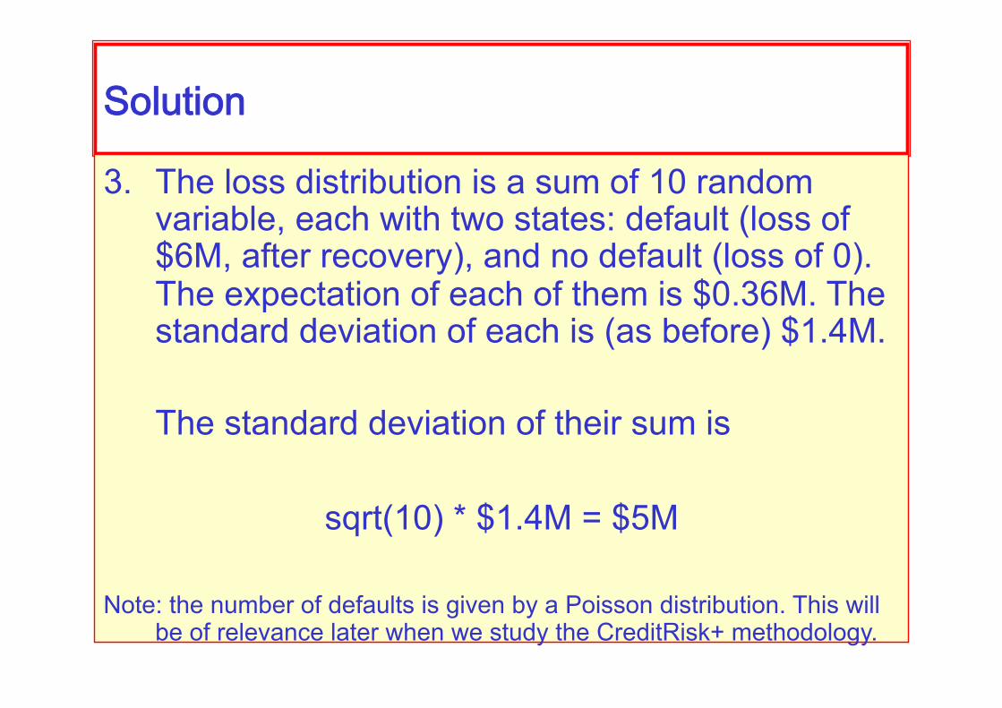
3. The loss distribution is a sum of 10 random variable, each with two states: default (loss of $6M, after recovery), and no default (loss of 0). The expectation of each of them is $0.36M. The standard deviation of each is (as before) $1.4M.
The standard deviation of their sum is
sqrt(10) * $1.4M = $5M
Note: the number of defaults is given by a Poisson distribution. This will be of relevance later when we study the CreditRisk+ methodology.
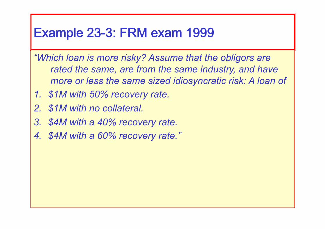
Example23-3:FRMexam1999
“Which loan is more risky? Assume that the obligors are rated the same, are from the same industry, and have more or less the same sized idiosyncratic risk: A loan of
1. $1M with 50% recovery rate. 2. $1M with no collateral. 3. $4M with a 40% recovery rate. 4. $4M with a 60% recovery rate.”

Example23-3:FRMexam1999“Which loan is more risky? Assume that the obligors are rated the same,
are from the same industry, and have more or less the same sized idiosyncratic risk: A loan of
1. $1M with 50% recovery rate. 2. $1M with no collateral. 3. $4M with a 40% recovery rate. 4. $4M with a 60% recovery rate.”
The expected exposures times expected LGD are: 1. $500,000 2. $1M 3. $2.4M. Riskiest. 4. $1.6M

Example23-4:FRMExam1999.
“Which of the following conditions results in a higher probability of default?
1. The maturity of the transaction is longer 2. The counterparty is more creditworthy 3. The price of the bond, or underlying security in the case
of a derivative, is less volatile. 4. Both 1 and 2.”

Example23-4:FRMExam1999.“Which of the following conditions results in a higher probability of
default? 1. The maturity of the transaction is longer 2. The counterparty is more creditworthy 3. The price of the bond, or underlying security in the case of a
derivative, is less volatile. 4. Both 1 and 2.”
Answer 1. True 2. False, it should be “less”, nor “more” 3. The volatility affects (perharps) the value of the portfolio, and hence
exposure, but not the probability of default (*)

Expectedlossoverthelifeoftheasset
Expected and unexpected losses must take into account, not just a static picture of the exposure to one cash flow, but the variation over time of the exposures, default probabilities, and express all that in today’s currency.
This is done as follows: the PV ECL is given by

Expectedloss:anapproximation
Rewrite:
Eachisreplacedbyanamountindependentoftime:theiraverage
Eachnumberchangeswithtime
Note:inthebook,theterm(1-f)isassumedtobeindependentoftime.Insomesituations,suchascommercialmortgages,thiswillunderestimatethecreditrisk.

Aswap

Theportfolio
5 year swap BBB counterparty $100M notional 6% annual interest rate (discount factor) 45% recovery rate Annual periods

Summary

CalculationforaBond
Aworked-outexample

Asimplebond
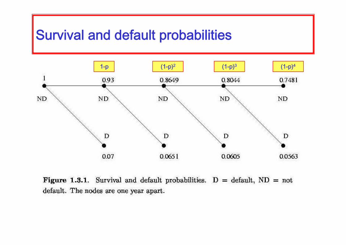
Survivalanddefaultprobabilities
1-p (1-p)2 (1-p)3 (1-p)4

Expectedlosscalculation
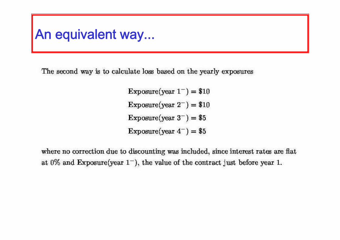
Anequivalentway...

...continued

Theunexpectedloss
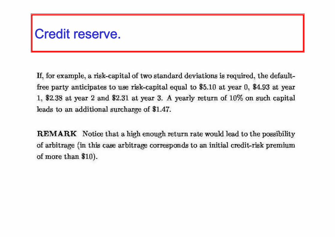
Creditreserve.

CreditVaR
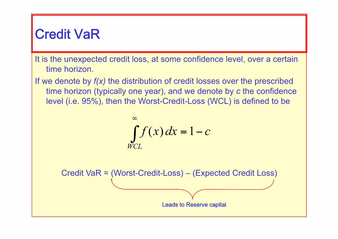
It is the unexpected credit loss, at some confidence level, over a certain time horizon.
If we denote by f(x) the distribution of credit losses over the prescribed time horizon (typically one year), and we denote by c the confidence level (i.e. 95%), then the Worst-Credit-Loss (WCL) is defined to be
Credit VaR = (Worst-Credit-Loss) – (Expected Credit Loss)
CreditVaR
LeadstoReservecapital

Example23-5:FRMexam1998
A risk analyst is trying to estimate the Credit VaR for a risky bond. The Credit VaR is defined as the maximum unexpected loss at a confidence level of 99.9% over a one month horizon. Assume that the bond is valued at $1M one month forward, and the one year cumulative default probability is 2% for this bond, what is your estimate of the Credit VaR for this bond assuming no recovery? 1. $20,000 2. 1,682 3. 998,318 4. 0
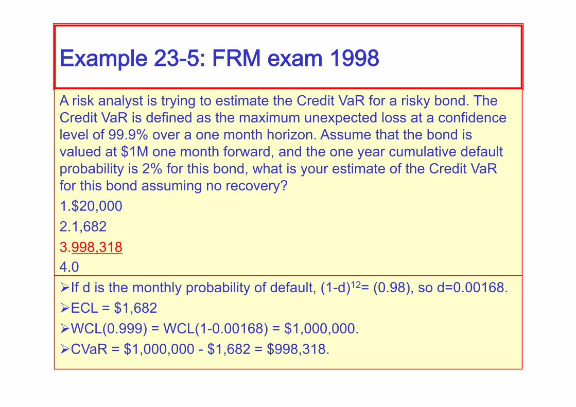
Example23-5:FRMexam1998A risk analyst is trying to estimate the Credit VaR for a risky bond. The Credit VaR is defined as the maximum unexpected loss at a confidence level of 99.9% over a one month horizon. Assume that the bond is valued at $1M one month forward, and the one year cumulative default probability is 2% for this bond, what is your estimate of the Credit VaR for this bond assuming no recovery? 1. $20,000 2. 1,682 3. 998,318 4. 0 If d is the monthly probability of default, (1-d)12= (0.98), so d=0.00168. ECL = $1,682 WCL(0.999) = WCL(1-0.00168) = $1,000,000. CVaR = $1,000,000 - $1,682 = $998,318.
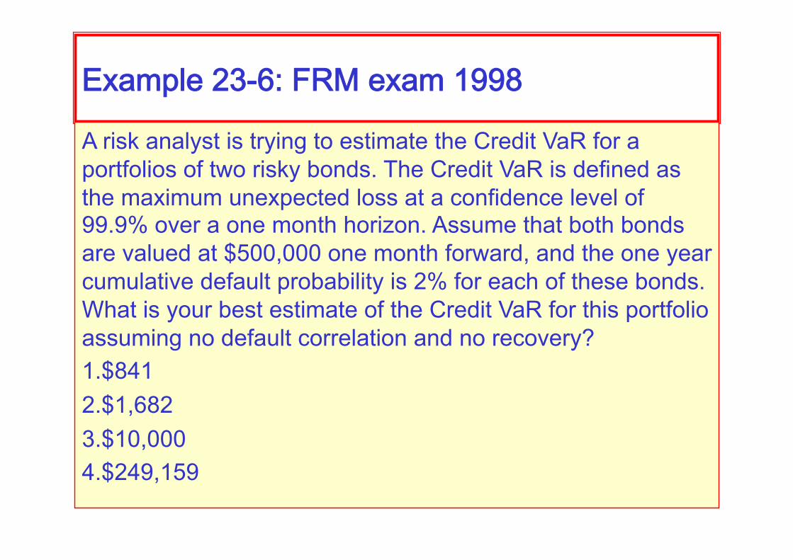
Example23-6:FRMexam1998
A risk analyst is trying to estimate the Credit VaR for a portfolios of two risky bonds. The Credit VaR is defined as the maximum unexpected loss at a confidence level of 99.9% over a one month horizon. Assume that both bonds are valued at $500,000 one month forward, and the one year cumulative default probability is 2% for each of these bonds. What is your best estimate of the Credit VaR for this portfolio assuming no default correlation and no recovery? 1. $841 2. $1,682 3. $10,000 4. $249,159
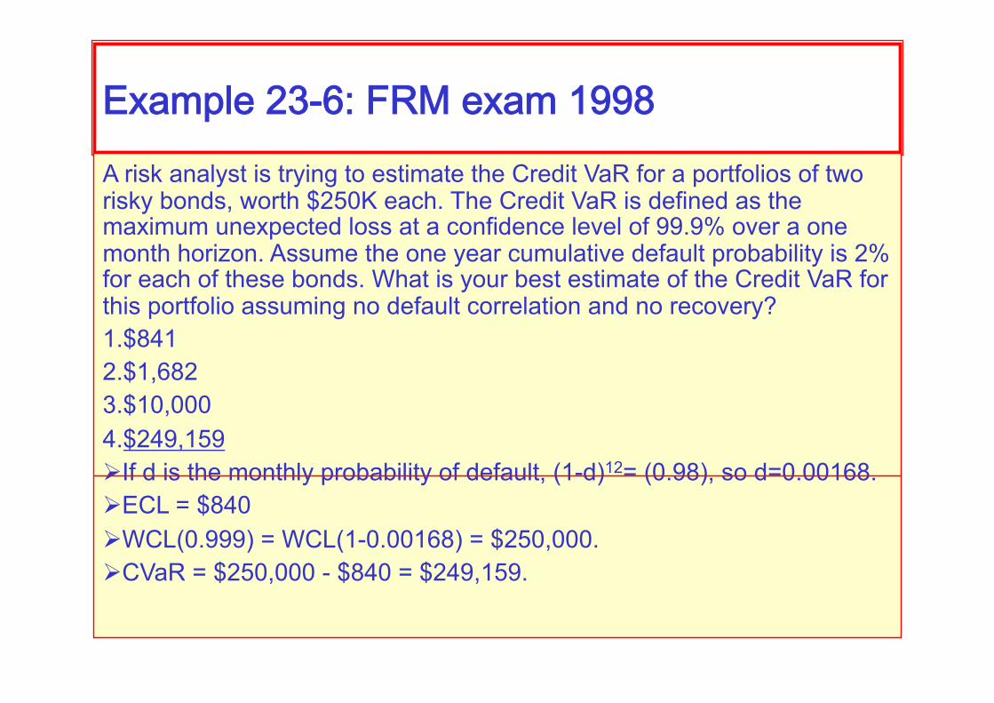
Example23-6:FRMexam1998A risk analyst is trying to estimate the Credit VaR for a portfolios of two risky bonds, worth $250K each. The Credit VaR is defined as the maximum unexpected loss at a confidence level of 99.9% over a one month horizon. Assume the one year cumulative default probability is 2% for each of these bonds. What is your best estimate of the Credit VaR for this portfolio assuming no default correlation and no recovery? 1. $841 2. $1,682 3. $10,000 4. $249,159 If d is the monthly probability of default, (1-d)12= (0.98), so d=0.00168. ECL = $840 WCL(0.999) = WCL(1-0.00168) = $250,000. CVaR = $250,000 - $840 = $249,159.

Solutionto23-6
As before, the monthly
d=0.00168
Default Probability Loss pxL
2 bonds d2=0.00000282 $500,000 $1.4
1 bond 2d(1-d)=0.00336 $250,000 $839.7
0 bonds (1-d)2=0.9966 0 0
The 99.9 loss quantile is about
$500,000 WCL=$250,000
EL=$839.70
CVaR=$250,000-$839.70
=249,159

Exercise
Credit VaR
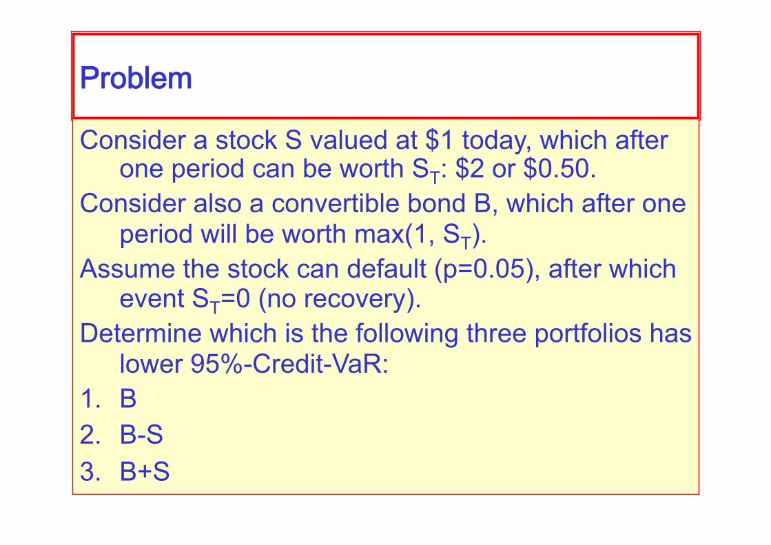
Problem
Consider a stock S valued at $1 today, which after one period can be worth ST: $2 or $0.50.
Consider also a convertible bond B, which after one period will be worth max(1, ST).
Assume the stock can default (p=0.05), after which event ST=0 (no recovery).
Determine which is the following three portfolios has lower 95%-Credit-VaR:
1. B 2. B-S 3. B+S

Goodrich
Calculating credit exposure

CreditVaR
Credit Exposure How much one can lose due to counterparty
default max( Swap Valuet , 0 )
CreditVaR
99% Credit VaR Sort losses and take the 99’th percentile

ExpectedShortfall
Expected Loss given 99% VaR Take the average of the exposure greater than
99% percentile.

Simulation
Monte Carlo simulation 10,000 simulations Simulate
Interest Rates Credit Spreads

InterestRates
Black-Karasinski Model
Tenor Init. IR Mean Vol 0.5yrs 8.18% 7.99% 5.98%
10yrs 10.56% 8.93% 5.64%
Est. from Bonds

Spreads
Vasicek Model
Tenor Init. IR Mean Vol 5yrs 2.4% 2.546% 0.535%

Algorithm
IR-Spread Choleski Decomposition Sample from Normal distribution Interest Rate-Spread Corr
1 0.9458 0.53
1 0.53
1 Corr of 6mo and 10yr rate
Est. from Bond Data
Corr of spread to 5yr IR
Est. from New Car Sales and
Bond rates 71-83

Algorithm
Iterate the Black-Karasinski Calculate the Value of the Swap as the difference
of the values of Non-Defaultable Fixed and Floating Bonds
After 10,000 calculate the credit VaR and the expected shortfall

Simulation:CreditExposure

Simulation:ExpectedShortfall

Creditmodels

PortfolioCreditRiskModels
CreditMetrics JPMorgan
CreditRisk+ Credit Suisse
KMV KMV
CreditPortfolioView McKinsey
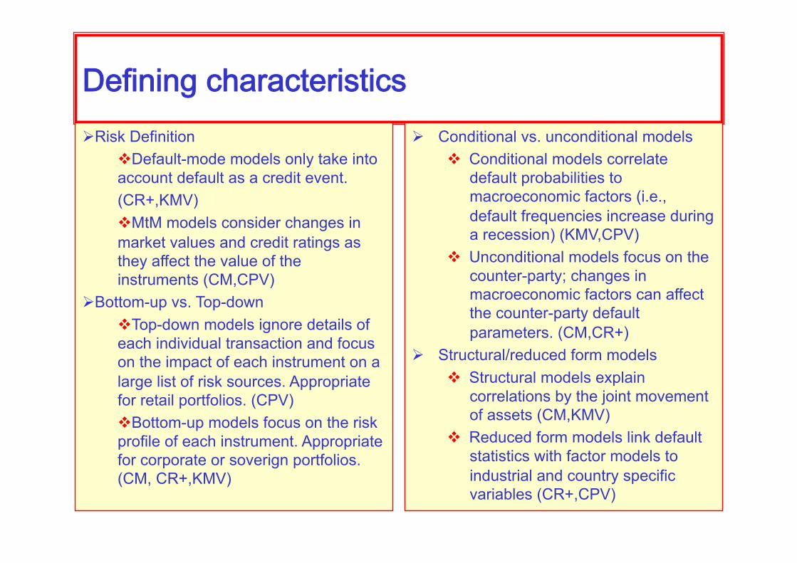
Definingcharacteristics Risk Definition
Default-mode models only take into account default as a credit event. (CR+,KMV) MtM models consider changes in market values and credit ratings as they affect the value of the instruments (CM,CPV)
Bottom-up vs. Top-down Top-down models ignore details of each individual transaction and focus on the impact of each instrument on a large list of risk sources. Appropriate for retail portfolios. (CPV) Bottom-up models focus on the risk profile of each instrument. Appropriate for corporate or soverign portfolios. (CM, CR+,KMV)
Conditional vs. unconditional models Conditional models correlate
default probabilities to macroeconomic factors (i.e., default frequencies increase during a recession) (KMV,CPV)
Unconditional models focus on the counter-party; changes in macroeconomic factors can affect the counter-party default parameters. (CM,CR+)
Structural/reduced form models Structural models explain
correlations by the joint movement of assets (CM,KMV)
Reduced form models link default statistics with factor models to industrial and country specific variables (CR+,CPV)

CreditMetrics Credit risk is driven by movements in bond ratings Analyses the effect of movements in risk factors to the exposure of
each instrument in the portfolio (instrument exposure sensitivity) Credit events are “rating downgrades”, obtained through a matrix of
migration probabilities. Each instrument is valued using the credit spread for each rating
class. Recovery rates are obtained from historical similarities. Correlations between defaults are inferred from equity prices,
assigning each obligor to a combination of 152 indices (factor decomposition)
All this information is used to simulate future credit losses. It does not integrate market and credit risk.
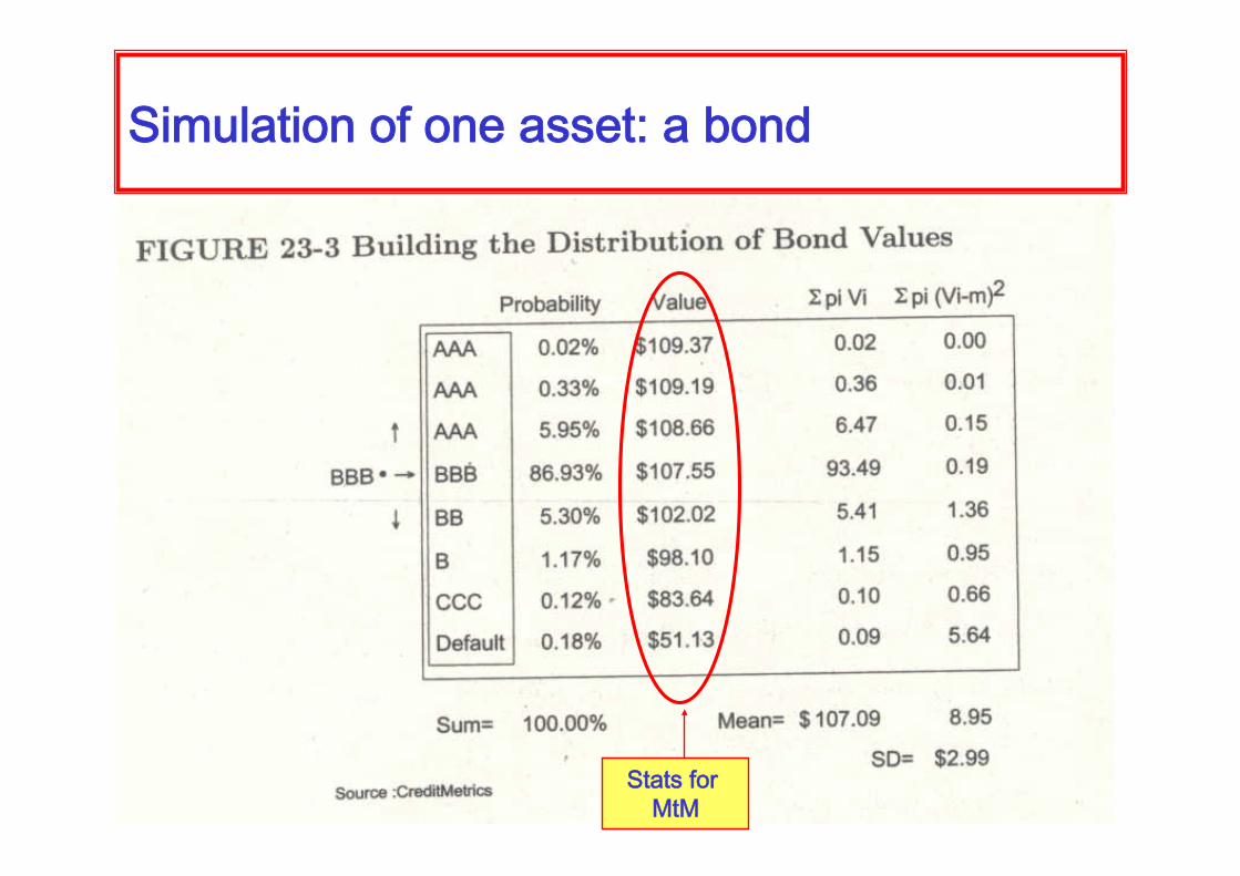
Simulationofoneasset:abond
StatsforMtM

Simulationofoneasset:abond
StatsforMtM
99% CVaR [$11 , $24]
2σ $6
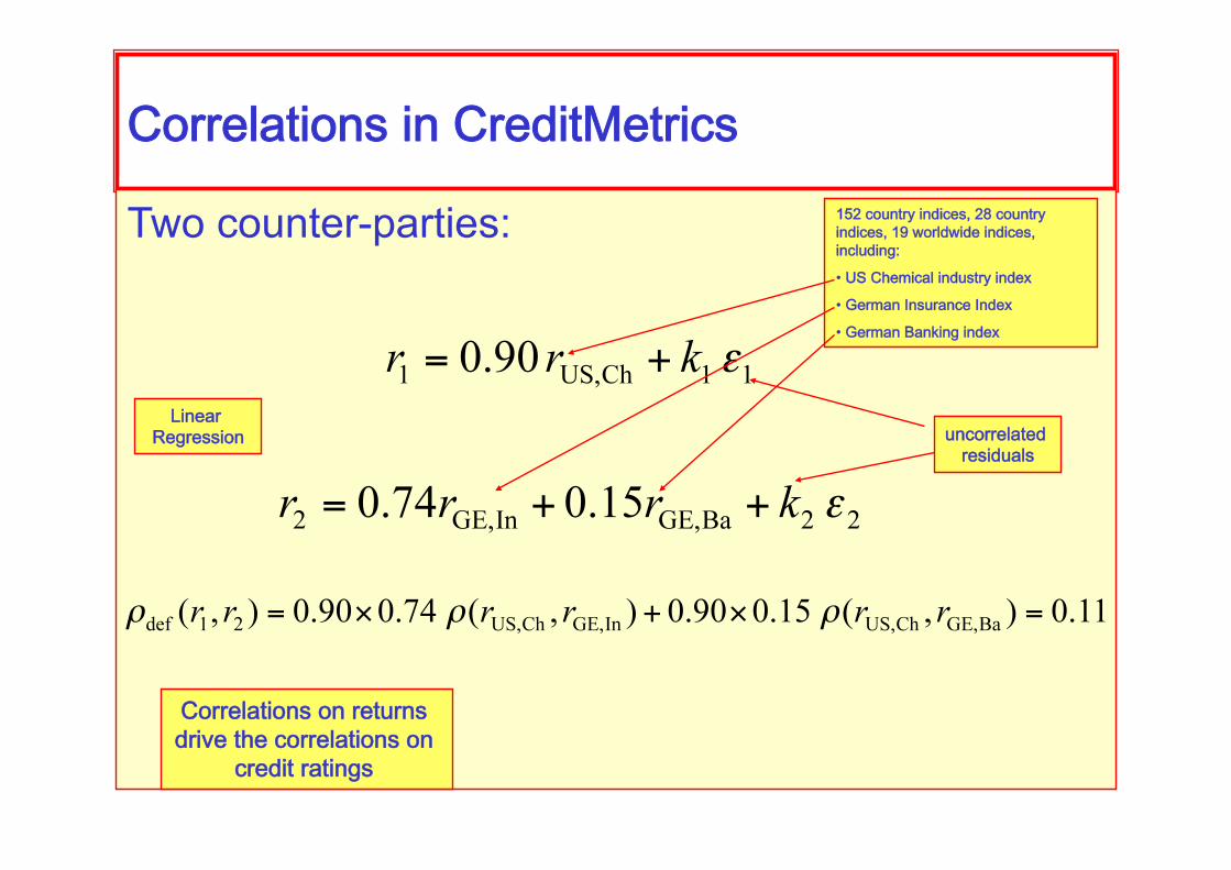
CorrelationsinCreditMetrics
Two counter-parties:
LinearRegression
152countryindices,28countryindices,19worldwideindices,including:
• USChemicalindustryindex• GermanInsuranceIndex• GermanBankingindex
uncorrelatedresiduals
Correlationsonreturnsdrivethecorrelationson
creditratings

Simulationofmorethanoneasset
Consider a portfolio consisting of m counterparties, and a total of n possible credit states.
We need to simulate a total of nm states; their multivariate distribution is given by their marginal distributions (as before) and the correlations given by the regression model.
To obtain accurate results, since many of these states have low probabilities, large simulations are often needed.
It does not integrate market and credit risk: losses are assumed to be due to credit events alone: for example, Swaps’ exposures are taken to be their expected exposures. Bonds are valued using today’s forward curve and current credit
spreads for generated future credit ratings.
Exercise
Pricing the Goodrich swap using the Credit Metrics framework

ThefullswapIf we consider the full swap, we need to consider the default process b
and the interest rate process r. The random variable that describes losses is given by
If we assume the credit process and the market process are independent, we get
This will overstimate the risk in the case that the default process and the market process are negatively correlated.

TheMonteCarloapproach
Correlation on market variables drive correlations of default events:
Then,
and
is calculated with Monte-Carlo techniques.

TheCreditMetricsApproach
Assume a 1 year time horizon, and that we wish to calculate the loss statistics for that time horizon.
Assume credit ratings with transition probabilities from BBB given by
andspreadsgivenby
AAA 25
AA 40
A 100
BBB 180
BB 250
B 320
CCC 500
Default
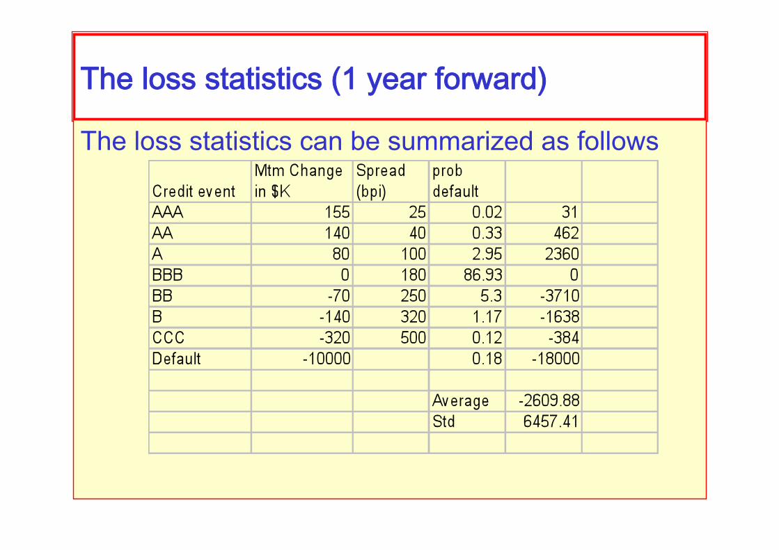
Thelossstatistics(1yearforward)
The loss statistics can be summarized as follows

Lossstatsoverthelifeoftheasset
Expected exposures, and exposure quantiles (in the case of this swap) will generally decrease over the life of the asset. They are pure market variables, which can be calculated with monte carlo methods.
Probability of default, and the probability of other credit downgrades, increase over the live of the asset. They are calculated, either with transition probability matrices, or with default probability estimations (Merton’s model, for instance)
Discount factors will also decrease with time, and are given by the discount curve.

Pricingthedeal
Assume the ECL=$50,000, and UCL=$200,000.
GR swap bps $K
Capital at Risk (UL, or CVAR) 200
Cost of capital is (15-8=7%)
Required net income (8 years) 112
Tax (40%) 75
Pretax net income 187
Operating costs 100
Credit Provision (ECL) 50
Hedging costs 0.50
Required revenue 0.50 327
CreditRisk+ Uses only two states of the world: default/no-default. But allows the default probability to vary with time. As we saw in the
review, if one considers only default/no-default states, the default probability must change with time to allow the credit spread to vary (otherwise, the spread is constant, and does not fit observed spreads)
Defaults are Poisson draws with the specified varying default probabilities.
Allows for correlations using a sector approach, much like CreditMetrics. However, it divides counter-parties into homogeneous sectors within which obligors share the same systematic risk factors.
Severity is modeled as a function of the asset; assets are divided into severity bands.
It is an analytic approach, providing quick solutions for the distribution of credit losses.
No uncertainty over market exposures.

CreditRisk+:introductoryconsiderationsIf we have a number of counter-parties A, each with a probability of
default given by a fixed PA, which can all be different, then the individual probability generating function is given by
If defaults are independent of each other, the generating function of all counter-parties is
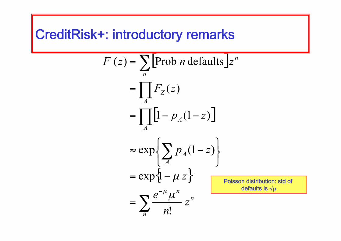
CreditRisk+:introductoryremarks
Poissondistribution:stdofdefaultsisõ

Thecaseforstochasticdefaultrates
Statistics from 1970 to 1996 Raiting Average default
probability (%) Standard deviation (%)
Aaa 0 0
Aa 0.03 0.01
A 0.1 0
Baa 0.12 0.3
Ba 1.36 1.3
B 7.27 5
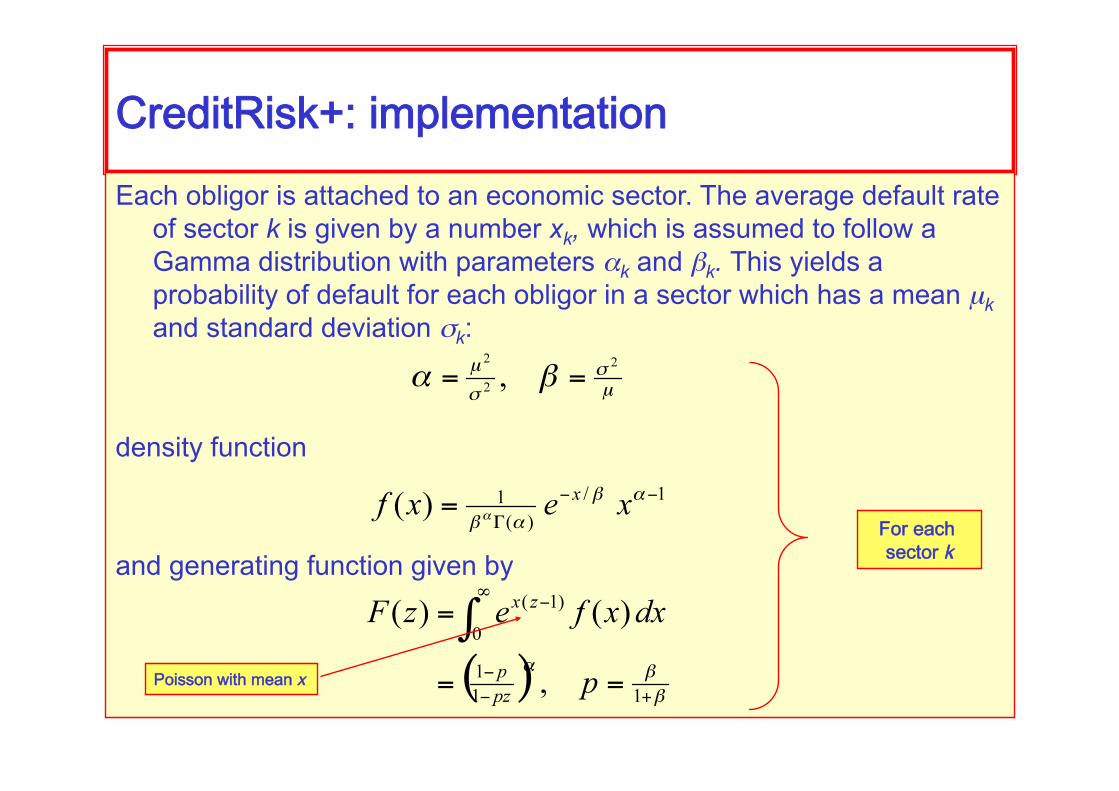
CreditRisk+:implementationEach obligor is attached to an economic sector. The average default rate
of sector k is given by a number xk, which is assumed to follow a Gamma distribution with parameters αk and βk. This yields a probability of default for each obligor in a sector which has a mean µk and standard deviation σk:
density function
and generating function given by Foreachsectork
Poissonwithmeanx

CreditRisk+
According to this, the probability of n defaults is given by the n’th term in the power series expansion of the generating function
Probabilityofndefaults
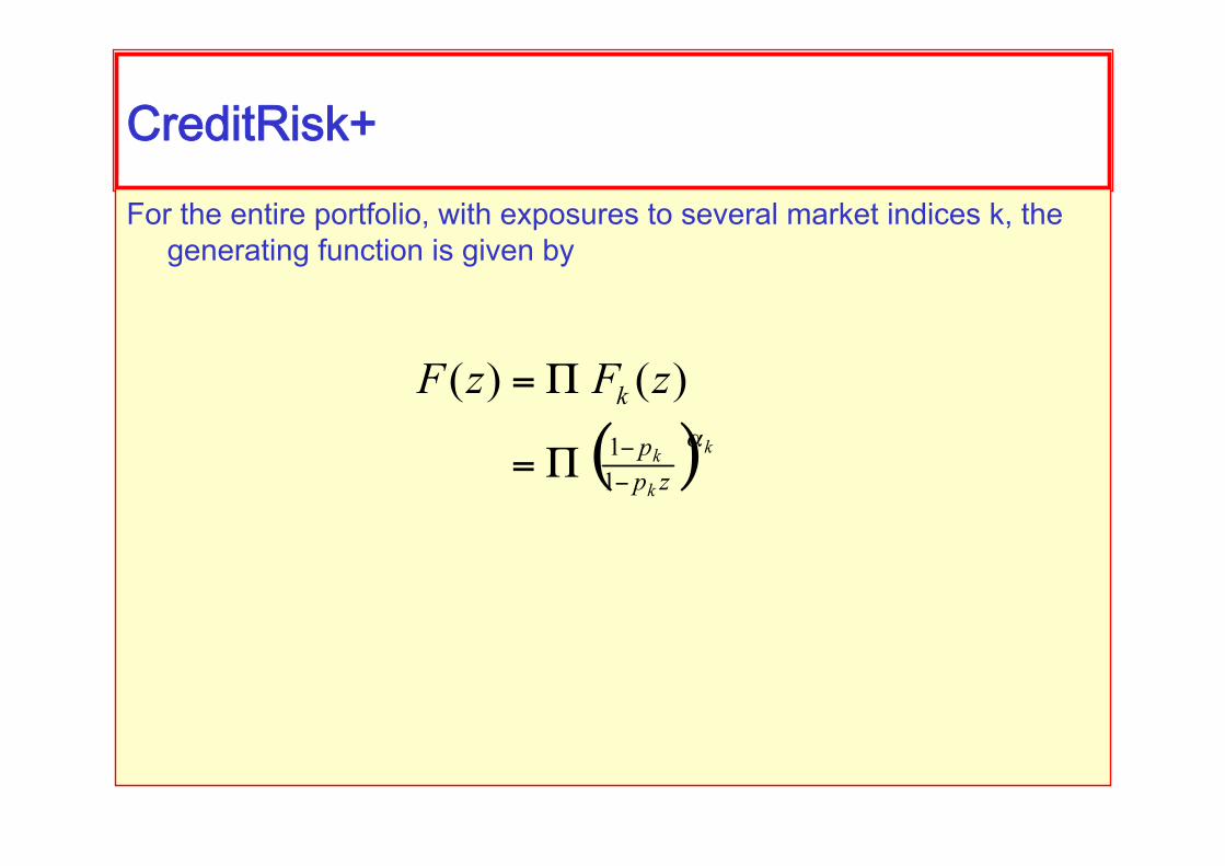
CreditRisk+For the entire portfolio, with exposures to several market indices k, the
generating function is given by
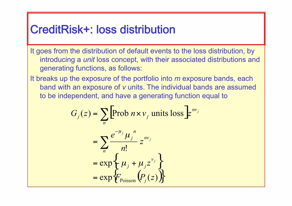
CreditRisk+:lossdistributionIt goes from the distribution of default events to the loss distribution, by
introducing a unit loss concept, with their associated distributions and generating functions, as follows:
It breaks up the exposure of the portfolio into m exposure bands, each band with an exposure of v units. The individual bands are assumed to be independent, and have a generating function equal to

CreditRisk+For the entire portfolio, with exposures to several market indices k, and
all exposure bands represented by levels j, we have a final explicit expression given by
KMVandtheMertonModel

TheMertonModel
Merton (1974) introduced the view that equity value is a call option on the value of the assets of the firm, with a strike price equal to the firm’s debt.
In particular, the stock price embodies a forecast of the firm’s default proabilities, in the same way that an option embodies an implied forecast of the option being exercised.
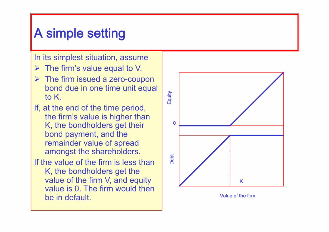
AsimplesettingIn its simplest situation, assume The firm’s value equal to V. The firm issued a zero-coupon
bond due in one time unit equal to K.
If, at the end of the time period, the firm’s value is higher than K, the bondholders get their bond payment, and the remainder value of spread amongst the shareholders.
If the value of the firm is less than K, the bondholders get the value of the firm V, and equity value is 0. The firm would then be in default. Valueofthefirm
K
Debt
0
Equity

Equityvaluesandoptionprices
In our simple example before, stock value at expiration is
Since the firm’s value equals equity plus bonds, we have that the value of the bond is
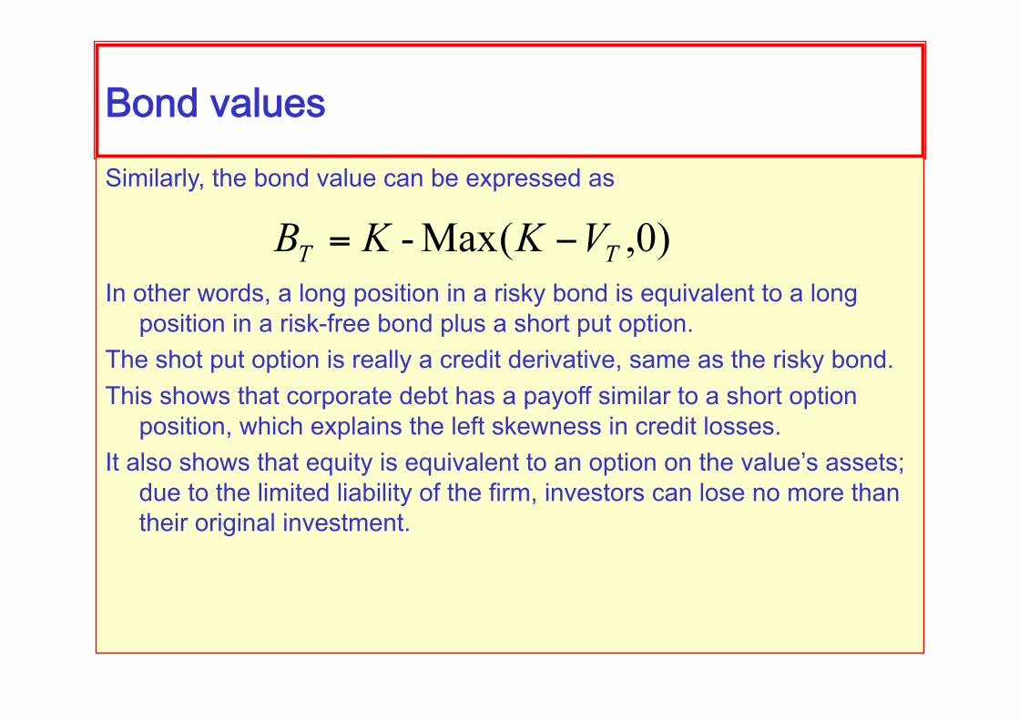
BondvaluesSimilarly, the bond value can be expressed as
In other words, a long position in a risky bond is equivalent to a long position in a risk-free bond plus a short put option.
The shot put option is really a credit derivative, same as the risky bond. This shows that corporate debt has a payoff similar to a short option
position, which explains the left skewness in credit losses. It also shows that equity is equivalent to an option on the value’s assets;
due to the limited liability of the firm, investors can lose no more than their original investment.

PricingequityWe assume the firm’s value follows a geometric brownian motion
process
If we assume no transaction costs (including bankruptcy costs)
Since stock price is the value of the option on the firm’s assets, we can price it with the Black-Scholes methodology, obtaining
with Leverage:Debt/Valueratio Assetvolatility

AssetvolatilityIn practice, only equity volatility is observed, not asset volatility, which we
must derive as follows: The hedge ratio
yields a relationship between the stochastic differential equations for S and V, from where we get
and
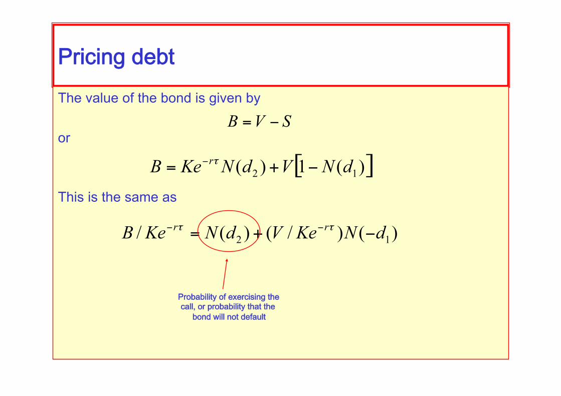
PricingdebtThe value of the bond is given by
or
This is the same as
Probabilityofexercisingthecall,orprobabilitythatthebondwillnotdefault

CreditLossThe expected credit loss is the value of the risk-free bond minus the risky
bond:
This is the same as
ECL=prob x Exposure x Loss-Given-Default
Probabilityofnotexercisingthecall,orprobabilitythatthebondwilldefault
PVofexpectedvalueofthefirmincaseofdefaultPVoffacevalueofthe
bond

Advantages
Relies on equity prices, not bond prices: more companies have stock prices than bond issues.
Correlations among equity prices can generate correlations among default probabilities, which would be otherwise impossible to measure.
It generates movements in EDP that can lead to credit ratings.

Disadvantages
Cannot be used for counterparties without traded stock (governments, for example)
Relies on a static model for the firm’s capital and risk structure: the debt level is assumed to be constant over the time
horizon. The extension to the case where debt matures are
different points in time is not obvious. The firm could take on operations that will increase stock
price but also its volatility, which may lead to increased credit spread; this is in apparent contradiction with its basic premise, which is that higher equity prices should be reflected in lower credit spreads.
KMV
KMV was a firm founded by Kealhofer, McQuown and Vasicek, (sold recently to Moody’s), which was a vendor of default frequencies for 29,000 companies in 40 different countries. Much of what they do is unknown.
Their method is based on Merton’s model: the value of equity is viewed as a call option on the value of the firm’s assets
Basic model inputs are: Value of the liabilities (calculated as liabilities (<1 year)
plus one half of long term debt) Stock value volatility Assets

Basicterms

BasicformulaMarketValueof
Assets
MarketValueofLiabilities
maturingattimet
Anapproximation

Example
Consider a firm with: $100M Assets $80M liabilities volatility of $10M (annualized) Distance from default is calculated as
Default probability is then 0.023 (using a gaussian)
Exercise

TheMertonModel
Consider a firm with total asset worth $100, and asset volatility equal to 20%.
The risk free rate is 10% with continuous compounding.
Time horizon is 1 year. Leverage is 90% (i.e., debt-to-equity ratio 900%) Find: The value of the credit spread. The risk neutral probability of default Calculate the PV of the expected loss.

CreditSpread
A leverage of 0.9 implies that
which says that K=99.46. Using Black-Scholes, we get that the call option is
worth S=$13.59. The bond price is then
for a yield of
or a credit spread of 4.07%.

OptionCalculation
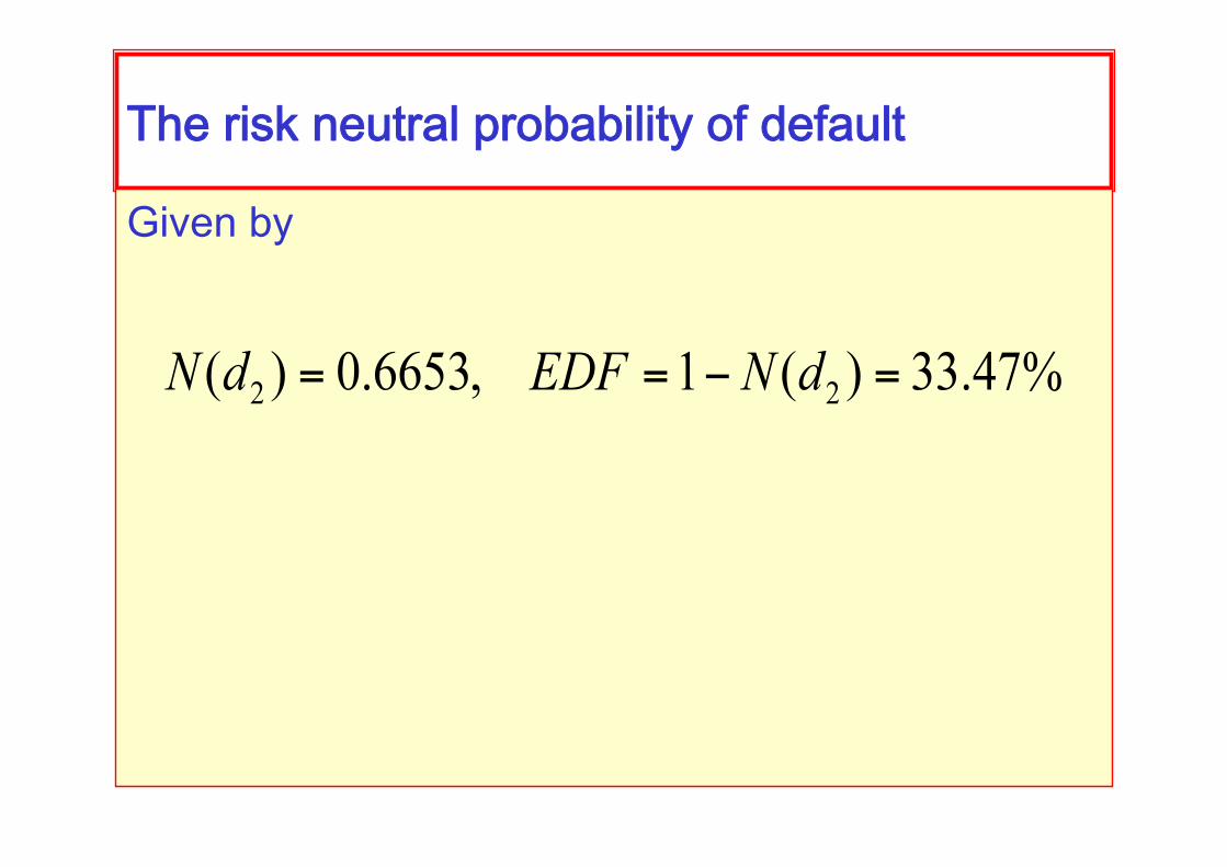
Theriskneutralprobabilityofdefault
Given by

Expectedloss
It is given by

Additionalconsiderations
Variations on the same problem: If debt-to-equity ratio is 233%, the spread is
0.36% If debt-to-equity ratio is 100%, the spread is about
0. In other words, the model fails to reproduce
realistic, observed credit spreads.

Exercise
Calibrating the asset volatility
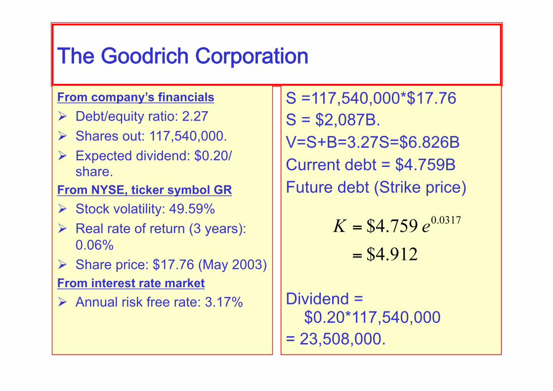
TheGoodrichCorporationFrom company’s financials Debt/equity ratio: 2.27 Shares out: 117,540,000. Expected dividend: $0.20/
share. From NYSE, ticker symbol GR Stock volatility: 49.59% Real rate of return (3 years):
0.06% Share price: $17.76 (May 2003) From interest rate market Annual risk free rate: 3.17%
S =117,540,000*$17.76 S = $2,087B. V=S+B=3.27S=$6.826B Current debt = $4.759B Future debt (Strike price)
Dividend = $0.20*117,540,000
= 23,508,000.

Bootstrappingassetvolatility
Slightlyhigh
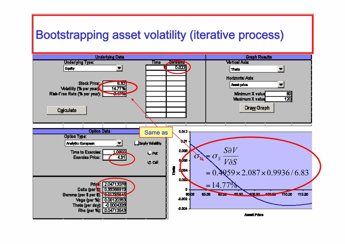
Bootstrappingassetvolatility(iterativeprocess)
Sameas
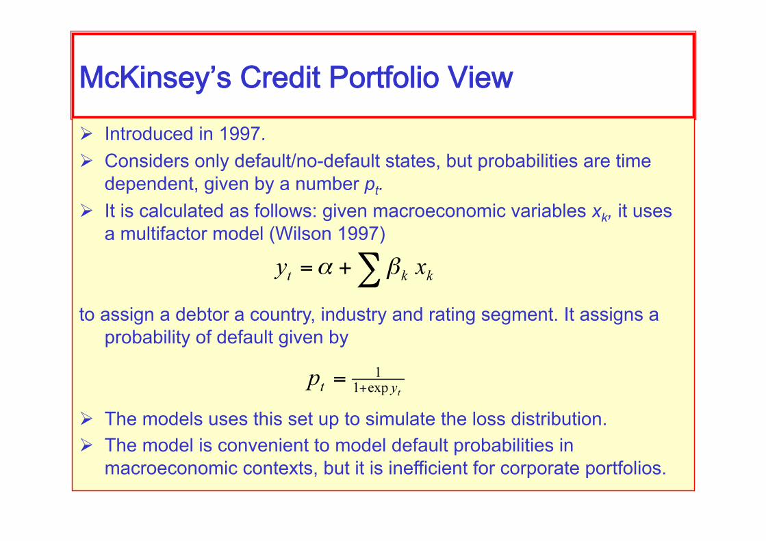
McKinsey’sCreditPortfolioView Introduced in 1997. Considers only default/no-default states, but probabilities are time
dependent, given by a number pt. It is calculated as follows: given macroeconomic variables xk, it uses
a multifactor model (Wilson 1997)
to assign a debtor a country, industry and rating segment. It assigns a
probability of default given by
The models uses this set up to simulate the loss distribution. The model is convenient to model default probabilities in
macroeconomic contexts, but it is inefficient for corporate portfolios.

Comparativestudy1 year horizon, 99% confidence Three models:
CM, CR+, Basel (8% deposit of loan notional)
Three portfolios, $66.3B total exposure each A: high credit
quality, diversified (500 names)
B: High credit, concentrated (100 names)
C: Low credit, diversified (500)
Assuming 0 correlations A B C
CM 777 2093 1989
CR+ 789 2020 2074
Basel 5304 5304 5304
Assuming correlations
CM 2264 2941 11436
CR+ 1638 2574 10000
Basel 5304 5304 5304
Higherdiscrepancybetweenmodels
Modelsarefairly
consistent
Correlationsincreasecreditrisk

Example23-7:FRMExam1999Which of the following is used to estimate the probability of default for a
firm in the KMV model? I. Historical probability of default based on the credit rating of the
firm (KMV have a method to assign a rating to the firm if unrated) II. Stock price volatility III. The book value of the firm’s equity IV. The market value of the firm’s equity V. The book value of the firm’s debt VI. The market value of the firm’s debt
a) I only b) II, IV and V c) II, III, VI d) VI only

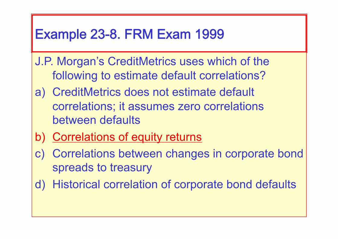
Example23-8.FRMExam1999
J.P. Morgan’s CreditMetrics uses which of the following to estimate default correlations?
a) CreditMetrics does not estimate default correlations; it assumes zero correlations between defaults
b) Correlations of equity returns c) Correlations between changes in corporate bond
spreads to treasury d) Historical correlation of corporate bond defaults

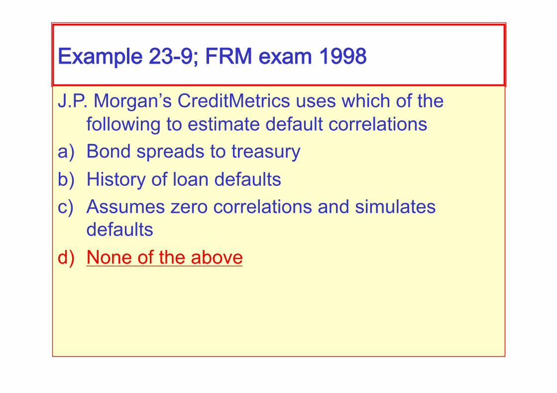
Example23-9;FRMexam1998
J.P. Morgan’s CreditMetrics uses which of the following to estimate default correlations
a) Bond spreads to treasury b) History of loan defaults c) Assumes zero correlations and simulates
defaults d) None of the above
Example23-9;FRMexam1998
J.P. Morgan’s CreditMetrics uses which of the following to estimate default correlations
a) Bond spreads to treasury b) History of loan defaults c) Assumes zero correlations and simulates
defaults d) None of the above
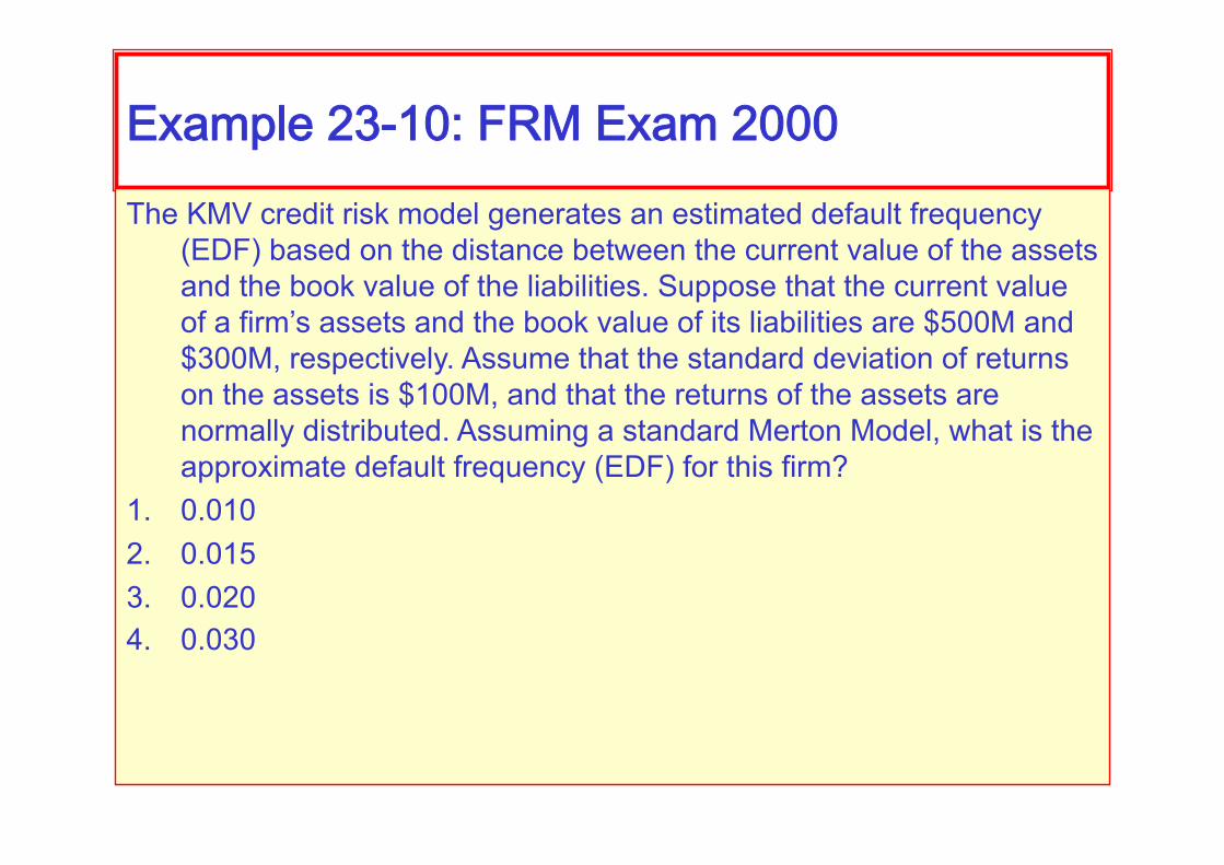
Example23-10:FRMExam2000The KMV credit risk model generates an estimated default frequency
(EDF) based on the distance between the current value of the assets and the book value of the liabilities. Suppose that the current value of a firm’s assets and the book value of its liabilities are $500M and $300M, respectively. Assume that the standard deviation of returns on the assets is $100M, and that the returns of the assets are normally distributed. Assuming a standard Merton Model, what is the approximate default frequency (EDF) for this firm?
1. 0.010 2. 0.015 3. 0.020 4. 0.030

Example23-10:FRMExam2000The KMV credit risk model generates an estimated default frequency (EDF)
based on the distance between the current value of the assets and the book value of the liabilities. Suppose that the current value of a firm’s assets and the book value of its liabilities are $500M and $300M, respectively. Assume that the standard deviation of returns on the assets is $100M, and that the returns of the assets are normally distributed. Assuming a standard Merton Model, what is the approximate default frequency (EDF) for this firm?
1. 0.010 2. 0.015 3. 0.020 4. 0.030
Distance from default is calculated as
Default probability is then 0.023 (using a gaussian)

Example23-11:FRMExam2000
Which one of the following statements regarding credit risk models is MOST correct?
1. The CreditRisk+ model decomposes all the instruments by their exposure and assesses the effect of movements in risk factors on the distribution of potential exposure.
2. The CreditMetrics model provides a quick analytical solution to the distribution of credit losses with minimal data input.
3. The KMV model requires the historical probability of default based on the credit rating of the firm.
4. The CreditPortfolioView (McKinsey) model conditions the default rate on the state of the economy.
CR+assumesfixedexposures

Example23-11:FRMExam2000
Which one of the following statements regarding credit risk models is MOST correct?
1. The CreditRisk+ model decomposes all the instruments by their exposure and assesses the effect of movements in risk factors on the distribution of potential exposure.
2. The CreditMetrics model provides a quick analytical solution to the distribution of credit losses with minimal data input.
3. The KMV model requires the historical probability of default based on the credit rating of the firm.
4. The CreditPortfolioView (McKinsey) model conditions the default rate on the state of the economy.
CMisasimulation

Example23-11:FRMExam2000
Which one of the following statements regarding credit risk models is MOST correct?
1. The CreditRisk+ model decomposes all the instruments by their exposure and assesses the effect of movements in risk factors on the distribution of potential exposure.
2. The CreditMetrics model provides a quick analytical solution to the distribution of credit losses with minimal data input.
3. The KMV model requires the historical probability of default based on the credit rating of the firm.
4. The CreditPortfolioView (McKinsey) model conditions the default rate on the state of the economy.
KMVusesthecurrentstockprice