Portfolio measurement, CAPM and APT

Susan ThomasIGIDR, Bombay

18 September, 2017

Goals

I Portfolio performance measuresI Factor models

Portfolio performance measurement

I A portfolio is defined as:I The total value of the portfolio.I The assets held in the portfolio.I The weight of each asset in the portfolio, wi .

I There are infinite ~w – how is performance measured?

Elements of performance evaluation framework

I The weights are optimised to deliver minimum σr for agiven E(r). (Markowitz)Insight: performance must include both E(rp) and σp.

I If E(rp) is the reward for holding only systematic risk, notunsystematic risk, thenInsight: Use βp ∗ σM as the risk measure.

I The one-fund separation theory suggests that efficientportfolios are a weighted average of E(rf ) and E(rM).Insight: performance of your choice of portfolio mustbenchmark against these.

I Returns on all alternative portfolios must be calculated tobe directly comparable.Insight: annualise returns, use the same method ofcompounding, the same currency units of value, includedividend payouts.

Questions of performance evaluation

1. What is a single measure that we use to compare theperformance of the portfolio?

2. What is the benchmark portfolio?3. What is the measure that captures whether the selected

portfolio performed “well” relevant to “the relevantbenchmark”?

4. Is the measure sufficient to differentiate between “actual”ability and “luck”?

Portfolio performance measures

I Sharpe’s ratio.I Treynor’s measure.I Jenson’s AlphaI Information RatioI Tracking ErrorI M2 measure

Mean-variance measures of performance, Sharpe’smeasure

I Sharpe’s measure:(r̄p − r̄f )

σp

I Returns is adjusted for the risk-free rate.I Risk is total risk of the portfolio returns. (Question: is this σ

of rp or (rp − rf )?)I It is an ordinal measure: it ranks different portfolios by their

return-risk performance.I The higher the Sharpe’s measure, the higher it’s rank in

performance.

Treynor’s measure

I Treynor’s measure:(r̄p − r̄f )

βp

I Returns is adjusted for the risk-free rate.I Risk is systemic risk of the portfolio returns. (Question: do

we have to worry about the rp vs. (rp − rf ) issue here?)I Higher Treynor’s measure→ higher the portfolio

performance ranking.

Jensen’s alpha

I Jensen’s measure:

αp = r̄p − r̄f − βp ∗ (r̄p − r̄f ))

I Here, the focus is on “excess returns”.Net of the returns predicted by the systemic risk of theportfolio, does this portfolio have more than zero returns?

I The larger the Jensen’s measure (also called the Alpha ofthe portfolio), the higher the rank in the portfolioperformance.

Information Ratio

I Information Ratio:αp

σ(ep)

I αp is Jensen’s measure for the portfolio.I σep is called the “tracking error” of the portfolio.I The larger the Information Ratio, the higher the rank in the

portfolio performance.

Tracking errorI Tracking Error (TE) is a measure of how well the portfolio

adheres to it’s stated scheme of investment.I TE measures how much the returns of the managed

portfolio “tracks” the returns of the stated benchmarkportfolio.

I Typically, all managed portfolios attract an investor set bystating the target portfolio allocation across differentassets: this is called the “stated scheme”.

I Example, “liquid funds” would be invested in short-termfixed income securities/fixed deposits.

I Example, “growth funds” would be invested in equity withhigh capital appreciation, rather than steady dividendpayouts.

I Example, “index funds” invest only in the stocks of theindex, and in the correct proportion.

I For a “well-managed portfolio”, TE is very small.I For any portfolio, TE can never be zero.

M2 measure

I The M2 measure helps to more directly compare thedifference between portfolio performance than the ranking.

I M2 is measured in two steps:1. Calculate σp, and adjust rp by the ratio:

A = σbenchmark/σp

Example: if σp = 3 ∗ σbenchmark, then r̂p,t = rp,t/32. Then, the performance measure is:

M2 = r̂p − rbenchmark

HW: calculate performance measures

Portfolio, P Market, Mr̄ 35% 28%β 1.2 1.0σ 42% 30%σep 18% 0%

I What is the Sharpe’s, Treynor, Jenson, Information Ratiomeasures for Portfolio P?

I Does P outperform the market using any of thesemeasures – if so, by which measure does P outperform?

Summarising performance measures

I Sharpe’s measure: (r̄p−r̄f )σp

I Treynor’s measure: (r̄p−r̄f )βp

I Jenson’s Alpha: αp = r̄p − r̄f − βp ∗ (r̄p − r̄f ))

I Information Ratio: αpσ(ep)

I M2 measure: M2 = r̂p − rbenchmark where r̂p is returnsadjusted for the ratio σbenchmark/σp

I A measure is used in different situations as portfolioperformance.What to use, where and when?

When performance is measured for the wholeinvestment

I If the portfolio being evaluated is the whole investment,then Sharpe’s measure is the best measure.

I Here, all that matters is whether the E(r) is commensuratewith the total expected risk of the investment portfolio.

When performance is measured for a part of theinvestment portfolio

I Question: what is the correct allocation of fresh funds tothe portfolio?

I Assumption: the full portfolio is well diversified, and hasonly systemic risk.In that case, the risk of the total investment is likely to bethe market index.

I Here, the best measure is Treynor’s measure.It identifies excess return for higher systematic risk.

A portfolio held with a index fund

I An index fund (equivalent to the one-fund of the one-fundseparation theorem) is optimally diversified.

I If fresh funds have to be allocated to any portfolio, then thenew portfolio must provide αp > 0.

I This must be adjusted for the risk of the portfolio over theindex risk.

I The measure to use here is the information ratio: αp/σep

Example of the above case: partial indexation

I A fund broadly tracks the index fund, but outperforms theindex. How can this happen?

I Two cases:I ‘Closet indexation’ - 80% in index, 20% is actively managed.I ‘Index+ funds’ - basically an index fund, some stocklending,

some index arbitrage, to juice up returns.I IR is a very useful measure here:

How much do you outperform, per unit TE incurred?

HW: Using measures

I Indian indexes: Nifty, Nifty Junior, CMIE CospiI Overseas: S&P 500, FTSE-100I An internationally diversified portfolio: 20% in India, 60% in

the US, 20% in the UK.

Compute and compare their Sharpe’s ratio. Sounds easy?

Implementation problems

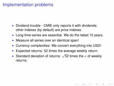
I Dividend trouble - CMIE only reports it with dividends;other indexes (by default) are price indexes.

I Long time-series are essential. We do the latest 10 years.I Measure all series over an identical span!I Currency complexities: We convert everything into USD!I Expected returns: 52 times the average weekly return.I Standard deviation of returns:

√52 times the σ of weekly

returns.

Sharpe’s ratio of some portfolios, 2008

Mean SD SRNifty 14.69 26.30 0.56

Junior 19.55 31.83 0.61COSPI 20.18 27.02 0.75

S&P 500 5.35 16.87 0.32FTSE-100 4.66 16.33 0.29Intnl divn 6.99 15.06 0.46

HW: What was the actual average performance of theseindexes in the following five year period?

Factor models

Statistical vs. theoryI Factor models are statistical models.I Problem: There exists n assets, i = 1,2, . . . ,n. Find a

single factor, f , such that

ri = ai + bi f + εi

E(εi) = 0E(εi , f ) = 0

I This factor is common to all the assets.I The factor affects the price of one asset through its mean,

variance and covariance with other assets:

E(ri) = ai + biE(f )

σ2i = b2

i σ2f + σ2

εi

σij = bibjσ2f where

bi = cov(ri , f )/σ2f

I The factor weight differs for different assets.

Example: CAPM as the first single factor model

I CAPM is a single factor model with excess returns on themarket portfolio as the factor:

E(ri − rf ) = βiE(rM − rf )

I Here, the single factor is identified as the market portfolio.The above formula is sometimes called the single indexmarket model (SIMM) or the market model.

I The single factor is supposed to be the SML marketportfolio m.Implementation: use the market index as the marketportfolio.

I Roll, 1977: criticism of small changes in the market returns

From CAPM to factor modelsI CAPM has a single factor – for “systematic risk” – common

across all stocks.Everything else is stock specific or unsystematic.

I Empirical observation: single factors capture a relativelysmall fraction of σr .Example: in the best case, market returns captures upto35% of σp.

I Observation 1: covariance between assets tend to behigher.Covariance between portfolios are much higher.

I Observation 2: covariance tends to be clustered.For example, returns of stocks from a given industry havea greater covariance than with stocks from other industries.

I Can we exploit these observations to get a better pricingmodel?Solution: Multi-factor models.

From CAPM to factor modelsI CAPM has a single factor – for “systematic risk” – common

across all stocks.Everything else is stock specific or unsystematic.

I Empirical observation: single factors capture a relativelysmall fraction of σr .Example: in the best case, market returns captures upto35% of σp.

I Observation 1: covariance between assets tend to behigher.Covariance between portfolios are much higher.

I Observation 2: covariance tends to be clustered.For example, returns of stocks from a given industry havea greater covariance than with stocks from other industries.

I Can we exploit these observations to get a better pricingmodel?Solution: Multi-factor models.

Multi-factor models

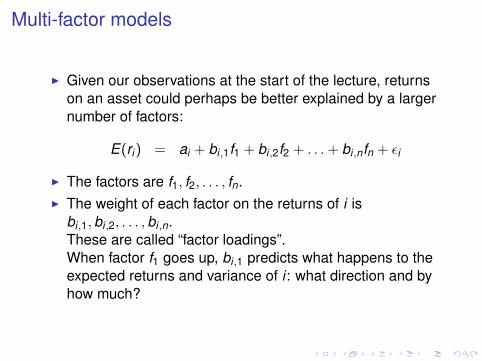
I Given our observations at the start of the lecture, returnson an asset could perhaps be better explained by a largernumber of factors:

E(ri) = ai + bi,1f1 + bi,2f2 + . . .+ bi,nfn + εi

I The factors are f1, f2, . . . , fn.I The weight of each factor on the returns of i is

bi,1,bi,2, . . . ,bi,n.These are called “factor loadings”.When factor f1 goes up, bi,1 predicts what happens to theexpected returns and variance of i : what direction and byhow much?

The econometric approach to factor models

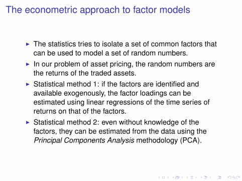
I The statistics tries to isolate a set of common factors thatcan be used to model a set of random numbers.

I In our problem of asset pricing, the random numbers arethe returns of the traded assets.

I Statistical method 1: if the factors are identified andavailable exogenously, the factor loadings can beestimated using linear regressions of the time series ofreturns on that of the factors.

I Statistical method 2: even without knowledge of thefactors, they can be estimated from the data using thePrincipal Components Analysis methodology (PCA).

The econometric approach to factor models

I The statistics tries to isolate a set of common factors thatcan be used to model a set of random numbers.

I In our problem of asset pricing, the random numbers arethe returns of the traded assets.

I Statistical method 1: if the factors are identified andavailable exogenously, the factor loadings can beestimated using linear regressions of the time series ofreturns on that of the factors.

I Statistical method 2: even without knowledge of thefactors, they can be estimated from the data using thePrincipal Components Analysis methodology (PCA).

The PCA approach

I In a system which are highly correlated, there is likely to bea small set of independant sources of variation, which canbe explained by a few principal components.

I PCA is based on the analysis of the eigenvalues andeigenvectors of the variance–covariance matrix of returns,where

1. The first PC explains the greatest amount of the variation,the second explains the next greatest amount, etc.

2. Each PC is independent of each other.

Arbitrage Pricing Theory (APT) – an operationalmulti-factor model

I APT was developed by Stephen Ross, 1976:

ri = ai + bi,1f1 + bi,2f2 + bi,3f3 + . . .+ bi,nfn

I The factors f1, f2, . . . , fn described the asset returnsperfectly.The uncertainty in E(ri) is only due to the uncertainty inEf1, f2, . . . , fn.

I APT states that if there are k assets, and that k > n, thereare constants λ0, λ1, λ2, . . . , λn such that

r̄i = λ0 + bi,1λ1 + bi,2λ2 + bi,3λ3 + . . .+ bi,nλn

APT assumptions

I The assumptions of APT are that investors prefer largerreturns to less, given certain returns. It does not requirethe risk-preference assumptions of the CAPM.

I It assumes that a very large set of assets, k is very large,and that every asset i is different from another.

I It should be possible to construct portfolios of any set ofassets such that the portfolio has

1. zero risk, and2. zero net investment

In this case, the return on this portfolio should be therisk-free rate, rf .

I When you solve for the asset returns using this framework,you arrive at the APT.

Factors in APT

I The theory says nothing about what the factors are, norhow to find them.Therefore, the APT models are fully flexible, and can varywidely from implementation to implementation.

I The first implementation of the APT was a model wherethe factors are “derived” from the data directly. It was amodel with five selected factors. The factor with the largest“importance” was identified to be the market portfolio.

I The typical implementation of APT has between three to15 factors.

Factors in APT

I The theory says nothing about what the factors are, norhow to find them.Therefore, the APT models are fully flexible, and can varywidely from implementation to implementation.

I The first implementation of the APT was a model wherethe factors are “derived” from the data directly. It was amodel with five selected factors. The factor with the largest“importance” was identified to be the market portfolio.

I The typical implementation of APT has between three to15 factors.

Factors in APT

I The theory says nothing about what the factors are, norhow to find them.Therefore, the APT models are fully flexible, and can varywidely from implementation to implementation.

I The first implementation of the APT was a model wherethe factors are “derived” from the data directly. It was amodel with five selected factors. The factor with the largest“importance” was identified to be the market portfolio.

I The typical implementation of APT has between three to15 factors.

What factors are to be used?

I Exogenous factors: typically macro–economic variableslike interest rates, exchange rates, GDP growth, etc.

I Factors specific to the sample set: industry factors,financial and accounting data

I Factors estimated from the sample set itself: There aretechniques like factor analysis, principle componentanalysis that derive factors that are weighted averages ofthe data itself (ie, returns and/or linear/non–linear functionsof returns).Problem: These factors are typically treated asblack–boxes, and cannot be linked back to an economicvariable without effort. This becomes a problem whenthese models are to be used for prediction.

Homework: Data constraints on estimating assetpricing models

I Leunberger, pages 212–222.

References

I Applied Multivariate Statistical Analysis, by Johnson andWichern: A good book to study PCA.

I Fama, French, Booth and Sinquefield, 1993: Expandingthe CAPM into a three factor model in a Financial AnalystsJournal paper.

I Ross, 1976: The seminal paper on APT in Journal ofEconomic Theory.

I Connor, 1984: The paper in Journal of Economic Theorythat worked out a form for the APT model.

References (contd.)

I Roll and Ross (1979, Journal of Finance), Chen, Roll andRoss (1986, Journal of Business), Lehman and Modest(1988, Journal of Financial Economics): Empiricalimplementations of the APT.

I Shanken (1982, Journal of Finance): The seminal paperon testing APT.

I Dybvig and Ross (1985, Journal of Finance): A theoreticalpaper on the testability of CAPM vs. APT.