portfolio selection under model uncertainty selection under model uncertainty 3 only partial moment...
TRANSCRIPT
manuscript No.(will be inserted by the editor)
Portfolio Selection under Model Uncertainty:
A Penalized Moment-Based Optimization Approach
Jonathan Y. Li · Roy H. Kwon
Received: date / Accepted: date
Abstract We present a new approach that enables investors to seek a reason-ably robust policy for portfolio selection in the presence of rare but high-impactrealization of moment uncertainty. In practice, portfolio managers face diffcultyin seeking a balance between relying on their knowledge of a reference financialmodel and taking into account possible ambiguity of the model. Based on the con-cept of Distributionally Robust Optimization (DRO), we introduce a new penaltyframework that provides investors flexibility to define prior reference models us-ing moment information and accounts for model ambiguity in terms of “extreme”moment uncertainty. We show that in our approach a globally-optimal portfo-lio can in general be obtained in a computationally tractable manner. We alsoshow that for a wide range of specifications our proposed model can be recastas semidefinite programs. Computational experiments show that our penalizedmoment-based approach outperforms classical DRO approaches in terms of bothaverage and downside-risk performance using historical data.
Keywords Portfolio selection · Model uncertainty · Distributionally robustoptimization · Penalty method
1 Introduction
Modern portfolio theory sheds light on the relationship between risk and returnover available assets, guiding investors to evaluate and achieve more efficient assetallocations. The theory requires specification of a model, e.g. a distribution of re-turns or moments of a distribution. To avoid any ambiguity, from here on “model”refers to the probability measure or moments that characterizes the stochasticnature of a financial market. In practice, practitioners cannot ensure the correct
Jonathan Y. Li · Roy H. KwonDepartment of Mechanical and Industrial Engineering, University of Toronto, 5 King’s CollegeRoad, Toronto, Ont., Canada M5S 3G8E-mail: [email protected]
Roy H. KwonE-mail: [email protected]

2 Jonathan Y. Li, Roy H. Kwon
choice of model due to the complex nature of model determination and validation.Thus, the need arises to take into account additional levels of uncertainty: modeluncertainty, also known as model “ambiguity”. Ellsberg [14] has also found thatdecision makers in fact hold aversion attitudes toward the ambiguity of models.As a classical example, even with lower expected return, investors have higherpreference for investments that are geographically closer due to their better un-derstanding of the return distribution. This finding implies that investors tend topay an additional ambiguity premium, if possible, in investing. Therefore, portfo-lio selection models that do not take into account this ambiguity-aversion attitudemay be unacceptable to such investors.
The classical maxmin approaches pioneered by Gilboa and Schmeidler [15] ac-count for investors’ ambiguity-aversion attitude by allowing investors to maximizethe expected utility of terminal wealth, while minimizing over a set of ambiguitymeasures. In practice, there exists some difficulty in implementing such an ap-proach. For example, in many cases, portfolio managers have particular views ofmarket movements based on their own expertise. They often quantify those viewsin terms of some models consistent with their confidence level for the markets andpursue returns based on the models. We may call such models “reference” models.The classical maxmin approach may generate portfolios that are too conservativefor an investor with some reference models, especially if the set of uncertain orambiguous models are much larger than the set of reference models. As a conse-quence, the performance of the portfolio generated using maxmin approach maybe fully unacceptable since it will not conform with the view of an investor withhis/her reference models.
Recent research of Anderson, Hansen, and Sargent [1], Uppal and Wang [31],and Maenhout [24] introduce a penalized maxmin framework that further incor-porates the information of a reference model into the classical maxmin setting. Tobe specific, a penalty function which measures discrepancy between probabilitymeasures is introduced to give weight (penalty) to each possible alternative modelaccording to its “deviation” from a prior reference model. Typically, the further analternative model is from the reference model, the larger the weight (penalty) it isassigned. Including such a penalty function into Gilboa and Schmeidler’s maxminformulation implicitly gives preference to the ambiguity measures closer to theinvestor’s reference measures, when minimizing over a set of possible measures.Based on the framework, managers are able to seek a balance between relying ontheir knowledge of a reference model and taking into account possible ambiguityof the model. In such a way, investors do not need to forgo all the potential gainassociated with their reference model while retaining a certain degree of aversiontowards ambiguity.
Classical penalized approaches assume that investors have some prior knowl-edge of the form of return distribution for a reference model. However, in prac-tice, one rarely has full distributional information of asset returns. As statedin Popescu [28], it is found that most reliable data comprise of only first andsecond order moments. Popescu further highlighted the fact that in RiskMetrics(www.riskmetrics.com) only covariance data are available. Aside from the aboveissue, even when probability distributions are given, they are typically under re-strictive forms, e.g. normality, which weakens robustness of solutions.
Recently, there is a growing body of research, so-called Distributionally RobustOptimization (DRO), that focus on stochastic optimization problems for which
Portfolio Selection under Model Uncertainty 3
only partial moment information of underlying probability measure is available.For example, El Ghaoui, Oks, and Oustry [13] considered a portfolio selectionproblem that minimizes worst-case value-at-risk of portfolios when only the meanand covariance information is available. Popescu [28] considered a wide range ofutility functions and studied the problem of maximizing expected utility of port-folios, given only mean and covariance values. Closer to the theme of this paperare the works of Natarajan, Sim, and Uichanco [26] and of Delage and Ye [12].In both papers, a piecewise linear concave utility function is considered; thoughin the latter paper emphasis is put on structuring an ellipsoidal set of mean vec-tors and a conic set of covariance matrices. Most DRO approaches are developedwith the purpose of achieving a computational tractable model so that they areapplicable to real world large-scale problems. Aside from the moment-based DROapproaches, several other facets of constructing a robust portfolio based on limitedstatistical information can also be found in Goldfarb and Iyengar [16], Tutuncuand Koenig [30], Calafiore [9], and Zhu and Fukushima [34].
In Delage and Ye [12], investors are allowed to describe their prior knowledgeof the financial market in terms of mean and covariance of the underlying distribu-tion. They further take into account the model ambiguity specifically in terms ofthe uncertainty of the mean and covariance. In their computational experiments,based on a simple statistical analysis Delage and Ye constructed a high-percentileconfidence region revolving around a pair of sampled mean and covariance. Theyfound that the respective performance is superior to the performance of the portfo-lio solved by an approach using a fixed pair of mean and covariance only. However,what remains to be investigated is the effect of the extreme values of moments thatfall outside the region on the overall portfolio performance. Due to its extreme-ness, moments at tail percentile may significantly change the portfolio selection.In addition, these “outliers” become ever non-negligible in modern portfolio riskmanagement as several severe losses in recent financial markets are due to thoserarely-happened events. Unfortunately, a “fixed-bound” DRO approach, like De-lage and Ye’s, may not provide a satisfactory solution since there is no clear ruleto decide a bound within this tail percentile. If including all “physically possi-ble” realizations of moments into the uncertainty set, one would obtain an overly“pessimistic” solution. Alternatively, if one specifies the uncertainty set based onhis/her confidence region of mean and covariance, this may leave investors fullyunguarded if the realized mean and covariance fall outside the uncertainty set. Inshort, any fixed bound can turn out to give a overly-conservative solution or asolution vulnerable to worst case scenarios.
The limitations of using a bounded set to describe uncertainty have also beenaddressed in the context of robust optimization (RO), in which no distributionalinformation is given except supports and performance is evaluated based solelyon the worst possible instance. Although the settings between DRO and RO aresomehow different, users of RO face similar difficulty of deciding an appropriatebound particularly for the extreme cases. To tackle this, Ben-Tal, Boyd, and Ne-mirovski [5] suggest a comprehensive robust approach that treats differently theinstances that fall into a “normal” range and the instances that fall outside of it.To be specific, for the instances within the “normal” region they treat the problemas a standard robust problem; for the instances outside the “normal” region theyconsider evaluating the problem based on a weighted-performance that furtheraccounts for the deviation of the instance from the “normal” range.
4 Jonathan Y. Li, Roy H. Kwon
Inspired by Ben-Tal, Boyd, and Nemirovski’s approach, we consider in thispaper an analogues scheme for overcoming difficulty within a DRO framework, e.g.Delage and Ye [12]. For the case that moments take values within the confidenceregion, a portfolio should be evaluated based on its worst-case performance so thatthe solution is robust with respect to likely outcomes that fall within the region. Forthe case that moments take values outside the confidence region, since evaluationbased on its worst-case performance can be overly-conservative, a portfolio shouldbe instead evaluated based on a weighted-performance that further accounts formoment deviation from the confidence region. To achieve a tractable model for thissetting, we employ two main theories of optimization that are commonly used inDRO approaches, duality theory and convex/semidefinite programming (see, Ben-Tal and Nemirovski [3]). There are three main steps in developing our approach.First, we apply the methodology of DRO to construct a portfolio selection modelfor which the moment uncertainty is specified by a bounded convex set. Then, wedesign a new penalty function that measures discrepancy between moments in andoutside the set. Finally, we incorporate such a penalty function into the portfolioselection model.
As a result, our method can be viewed as an extension of the classical penalizedminimax approaches, where the reference measure is replaced by the confidenceregion of reference moments and alternative measures are replaced by alternativemoments. Besides the possible modeling benefit, one other advantage of our penal-ized moment-based approach is its tractability, as a penalized distribution-basedapproach typically results in a computationally overwhelming optimization prob-lem unless some strong assumptions are made, e.g. normality, or discrete randomreturns (e.g. [9]). Without these assumptions, a sampling-based approximation istypically required to evaluate an integral with respect to a reference distributionfor a distribution-based approach. This could lead to a extremely large-scale prob-lem. In contrast, our problem is moment-based and thus is expected to be freefrom such a challenge. In this paper, we provide two computationally tractablemethods for solving the problem. The first method is developed using the famousellipsoid method well suited for a general convex formulation, and the second oneis based on semidefinite programming reformulations and state-of-art semidefiniteprogramming algorithms.
After submission of this article, we became aware of the work of Ben-Tal,Bertismas, and Brown [2], who addressed a similar issue of model ambiguity andconsidered also a penalized approach to tackle the issue of conservatism. A majordifference between their approach and ours is that they consider to penalize al-ternative models based on their distance to a reference distribution while in ourapproach we do not assume investors to have prior knowledge of a reference distri-bution and penalize alternative models instead based on the distance of moments.As addressed earlier, such a moment-based setting allows for additional modelingpower and maximizes the tractability of the resulting problem. Another main mo-tivation of our consideration of moment setting is that moments, e.g. mean andvariance, are usually more tangible quantity to practitioners and often easier forthem to express their perspective of market movements (see, e.g. [8]). Moreover,our methodology can in fact be carried over to the cases when the only interest-ing quantity to differentiate models is their respective expected value performance(see, e.g. [11]).
Portfolio Selection under Model Uncertainty 5
To examine the strength of our approach, we further specialize the penalizedproblem based on the portfolio selection model in Delage and Ye [12], and compareit with the approaches in [12] and [28], and with a sampled-based approach. Fromthe computational experiments on real-market data, we find that in most cases ourapproach outperforms other approaches and results in more risk-return efficientportfolio. We also find that the improvement of the performance becomes moresubstantial as the market becomes more volatile.
The structure of this paper is as follows. In section 2, we present a new pe-nalized distributionally robust approach which does not rely on full distributionalinformation and requires only the first two moments. In section 3, we provide so-lution methods for solving the problem and further specialize the problem to aparticular class of convex problems, i.e. semidefinite programming problems. Wethen consider variations and extensions of the problem such as frontier generation,incorporation of alternative moment structures, and extension to factor models insection 4. Finally, a numerical study is presented in section 5.
2 A Penalized Distributionally-Robust-Optimization Model
Throughout this paper, we consider a single-period portfolio optimization problem
infx∈X
EQ[G(wTx)], (1)
where Q denotes the probability measure of random returns w. For technical rea-sons, we consider the probability measure Q associated with measurable space(ℜn,B).1 An investor intends to optimize his/her overall wealth wTx accordingto a certain convex measure function G, where x ∈ ℜn is a wealth allocation vec-tor assigned over n assets associated with the vector of random returns w ∈ ℜn.The allocation vector x is subject to a convex feasible set X ⊆ ℜn, which is typi-cally specified by some real-life constraints, e.g. budget and short-sales restrictions.This formulation encompasses both the case of maximizing the utility of a portfolioand the case of minimizing a risk measure represented by a convex nondecreasingdisutility function. Without loss of generality, we uniformly adopt a minimizationnotation.
2.1 Motivation
In the classical penalized minmax framework, an investor is uncertain about theexact distributional form of the probability measure Q, and the information he/shecan provide about Q is that it belongs to a certain set Q. Occasionally, among allthe measures in the set Q the investor could have a particularly strong preferencefor a specific measure P and holds an aversion attitude towards other measuresin the set Q. In such cases, it is reasonable to treat the measure P as a referencemeasure and consider the following penalized minimax problem instead of (1)
infx∈X
supQ∈Q
{EQ[G(wTx)]− k · H(Q| P)}, (2)
1 B is Borel σ−algebra on ℜn.

6 Jonathan Y. Li, Roy H. Kwon
where H is a penalty function that satisfies
Q = P ⇔ H(Q| P) = 0,
Q = P ⇔ H(Q| P) > 0,
and the parameter k helps to adjust the level of penalty. The inner maximization(supQ∈Q) in (2) evaluates the worst-possible expectation value that reflects aninvestor’s aversion attitude towards the ambiguity of Q, while the penalty functionH adjusts the level of aversion towards each Q further based on its correspondenceto P. Typically, the magnitude of the penalty value is positively correlated withthe discrepancy between Q and P, and therefore the further Q is from P the lesslikely it is to be chosen for evaluating the expectation. This in essence leads toless-conservative portfolio selection.
In this section, we refine the above penalized concept into a moment-basedframework so that the requirement of a complete probability description can berelieved. Instead of using a single measure P, in the new framework an investorcan specify his/her preference measures via a set of first two moments (µc, Σc) ={(µi, Σi) | i ∈ C}, which can also be treated as the investor’s confidence region ofmoments. From here on, the notation Q(· ; µ,Σ) denotes a probability measureQ associated with mean µ and covariance Σ. The set Q that comprises all theambiguous measures Q shall be replaced by a set (µs, Σs) = {(µi, Σi) | i ∈ S}that comprises all pairs of ambiguous moments (µ,Σ) (of Q). Thus, if µ ∈ ℜd
and Σ ∈ ℜd×d then both the sets (µc, Σc) and (µs, Σs) are subsets of the spaceℜd × ℜd×d. Note that the confidence region of moments (µc, Σc) can be either asingleton or an uncountable set. Now, we reformulate the problem in terms of themoment-based framework
infx∈X
sup(µ,Σ)∈(µs,Σs),Q(· ; µ,Σ)
{EQ(· ; µ,Σ)[G(wTx)]− Pk( µ,Σ | µc, Σc )}.
In the above formulation, the function Pk is a newly-introduced function thatmeasures the discrepancy between a pair of moments (µ,Σ) and the set of momentsspecified in the confidence region (µc, Σc). We call such discrepancy as “momentsdiscrepancy” throughout the paper. Analogous to the function H, the function Pk
is assumed to satisfy the following property
(µ,Σ) ∈ (µc, Σc) ⇔ Pk( µ,Σ | µc, Σc ) = 0,
(µ,Σ) /∈ (µc, Σc) ⇔ Pk( µ,Σ | µc, Σc ) > 0.
Similarly, the magnitude of the functional Pk(·) is assumed to be positively cor-related with the moments discrepancy. Thus, the larger the moments discrepancybetween (µ,Σ) and (µc, Σc) is, the less likely it is for the measure Q(· ; µ,Σ)to be chosen for evaluating the expectation. From a modeling perspective, themoment-based problem provides a comprehensive treatment for an investor hold-ing different conservative attitudes towards the following three ranges within which(µ,Σ) possibly takes values:
– When the candidate mean and covariance (µ,Σ) stays within the confidenceregion (µc, Σc), the problem recovers the standard minmax setting. In otherwords, when an investor is certain about some realizations of moments, he/shenaturally holds strictly conservative attitude and pursues only robust perfor-mance of portfolio selection.
Portfolio Selection under Model Uncertainty 7
– When (µ,Σ) /∈ (µc, Σc) but is in the set (µs, Σs), this represents an “ambigu-ity” region that an investor seeks a balance between relying on his/her priorknowledge and properly hedging the risk of model uncertainty, where (µs, Σs)contains all “physically possible” realizations of moments. In this region, us-ing a standard minmax setting can lead to an impractical solution. Instead,the moment-based problem helps an investor to decide appropriate conserva-tiveness based on the possible performance deterioration resulting from each(µ,Σ) /∈ (µc, Σc). This leads to a less-conservative setting.
– When (µ,Σ) /∈ (µs, Σs), the moments are in a region with no “physically possi-ble” realizations. Therefore, the trading strategy is optimized without takinginto account this scenario when evaluating its worst-case performance. An in-vestor holds no conservative attitude for this region.
2.2 A Penalized Distributionally-Robust-Optimization Model
In this section, we further specialize the moment-based problem by refining thestructure of the penalty function Pk. We first consider two separate distance func-tions dµ : ℜd × ℜd → ℜ+, dΣ : ℜd×d × ℜd×d → ℜ+ that are used to measurethe deviation of (µ,Σ) from the confidence region (µc, Σc). Specifically, we de-fine dµ(µ, µc) := infν∈µc ||µ − ν|| and dΣ(Σ,Σc) := infσ∈Σc
||Σ − σ|| as distancefunctions, where the notation || · || denotes a norm that satisfies the propertiesof positive homogeneity and of subadditivity. From here on, for tractability weassume that the sets µc and Σc are closed, bounded and convex. In some cases,it can be useful to have the penalty function Pk depend non-linearly on the mo-ments discrepancy, and we assume only that Pk is jointly convex with respect todµ(µ, µc) and dΣ(Σ,Σc).
To implement the overall problem in a tractable manner, we now propose thefollowing penalized distributionally robust optimization model
(Pp) minx∈X
maxγ,µ,Σ,Q(· ; µ,Σ)
∫G(wTx)dQ(w)− rk(γ)
subject to infν∈µc
||µ− ν|| ≤ γ1 (3)
infσ∈Σc
||Σ − σ|| ≤ γ2 (4)
0 ≤ γ ≤ a. (5)
In the above model, the penalty function Pk is implemented using an alternativeconvex penalty function rk together with the constraints (3) and (4). The variableγ denotes the vector (γ1, γ2). The variables γ1, γ2 are introduced to bound themean-covariance discrepancy. The function rk is assumed to satisfy the propertiesof a norm and used to measure the magnitude of the vector γ and thus translatethe moments discrepancy into penalty. The constraint (5) provides a hard boundon γ and models the “physically possible” region (µs, Σs).
Our last two refinements of the model (Pp) are as follows. First, the objectivefunction G is assumed to be a piecewise-linear convex function
G(z) := maxj=1,...,J
{ajz + bj}.
8 Jonathan Y. Li, Roy H. Kwon
This general piecewise linear structure provides investors the flexibility to maxi-mize a piecewise linear utility function by setting aj = −cj and bj = −dj giventhe utility function u(z) := minj=1,...,J{cjz+dj}. This structure can also be easilyextended to model the popular CVaR risk measure and a more general optimizedcertainty equivalent (OCE) risk measure (see Natarajan, Sim, and Uichanco [26]).
Furthermore, the penalty function rk(γ) is assumed to admit the form
rk(γ) :=I∑
i=1
kiri(γ), ki ≥ 0, (6)
where each ri is a convex norm function. In this form, the penalty parameter k isexpanded from a scalar to a vector. This expansion allows for a more flexible way toadjust investors’ aversion towards model ambiguity based on particular structuresof (γ1, γ2). Thus, the index k in rk(·) should correspond to a vector (k1, ..., kI)at right-hand-side of (6). In addition, k2 > k1 means that k2i > k1i , i = 1, ..., I.We now consider how an investor may adjust his/her ambiguity-aversion attitudeusing (6) in the following example.
Example 1 Consider the penalized problem (Pp) with rk(γ) = k1γ1 + k2γ2 +k3||γ||2. By setting k3 = 0, ambiguity of mean and covariance can only be adjustedindependently. As an example, a risk-management oriented investor can be lesssensitive towards the ambiguity of mean and thus tends to increase the value ofk1; he however may hesitate to increase the value of k2 due to the concern ofunexpected volatility. On the other hand, a return-driven investor may do so inan opposite way. When k3 = 0, ambiguity of mean and covariance can be bothadjusted independently and dependently. Thus, for an investor who thinks thechance that both mean and covariance will fall outside the confidence region issmall, increasing k3 value serves the need.
Remark 1 Classical penalized approaches based on a relative entropy penalty func-tion can in fact be viewed as a special instance of our moment-based approach whenthe standard assumption of normality is made. The relevant discussion is providedin the appendix.
3 Solution Method and Computational Tractability
In this section, we first provide a general solution method based solely on theconvexity of the confidence region (µc, Σc). Later, we assume that the set (µc, Σc)is a conic set and focus on reformulating the problem (Pp) as a semidefinite pro-gramming problem.
3.1 Solutions via a General Convex Programming Approach
The goal of this section is to obtain a globally-optimal solution for the problem(Pp) in a computationally tractable manner. To help the discussion, we define firstthe following two functions
F(x, γ) := maxµ,Σ,Q(· ; µ,Σ)
{∫
G(wTx)dQ(w) | (3) ∼ (5)}, (7)
Portfolio Selection under Model Uncertainty 9
Sk(x, γ) := F(x, γ)− rk(γ).
Thus, Sk(x, γ) denotes the optimal value of (Pp), given k, x, γ. The solutionmethod is developed based on two observations. First, given fixed k, x, the func-tional Sk(x, γ) is concave with respect to γ. This concavity observation togetherwith the convexity of the feasible region X (of the wealth allocation vector x)allows us to reformulate the problem by exchanging the minx∈X and the maxγ ;thus, we can reformulate the problem (Pp) as follows
(Pν) max0≤γ≤a
ν(γ)− rk(γ),
where
ν(γ) := minx∈X
{ maxµ,Σ,Q(· ; µ,Σ)
{∫
G(wTx)dQ(w) | (3) ∼ (5)}}. (8)
In addition, the concavity observation also gives us the certificate that a localsearch method is sufficient to find a globally optimal γ∗ if ν(γ) can be evaluatedfor any γ. Our second observation is that given a fixed γ, there exists a computa-tionally tractable approach to solve the dual problem of the right-hand-side opti-mization problem in (8) and strong duality holds for the right-hand-side problem.That is, for fixed γ the functional ν(γ) can be efficiently evaluated. Combiningthese two observations, a direct search method (see Kolda, Lewis, and Torczon[20]) can be applied to solve (Pν). For such a two-dimensional problem with box-type of constraints, a straightforward approach that leads to global convergenceis to examine the steps along x, y-coordinate directions. If there exists a feasibleand improved direction, new iterate is updated; otherwise, bisect the four possi-ble steps and examine them again. Although a direct search method may not beas efficient as a derivative-based optimization method, the problem (Pν) shall besmall and simple enough to be tractable using such a method. Furthermore, ifonly the bound γ∗ = max(γ1, γ2) is of interest to penalize, the problem (Pν) thatunifies the bound γ1 = γ2 can be solved in polynomial time using a binary searchalgorithm (e.g., Chen and Sim [10]).
Up to now, we have only stated the two observations as a fact but have notjustified their validity. The first observation is proven in the Theorem 1, whichhinges heavily on the following lemma.
Lemma 1 Given that the distance functions dµ(·, µc), dΣ(·, Σc) are convex, letQα(· ; µα, Σα) (resp. Qβ(· ; µβ , Σβ)) denotes a probability measure that satisfiesdµ(µα, µc) ≤ αµ (resp. dµ(µβ , µc) ≤ βµ) for some αµ(resp. βµ) and dΣ(Σα, Σc) ≤αΣ (resp. dΣ(Σβ , Σc) ≤ βΣ) for some αΣ(resp. βΣ). Then, there exists a prob-ability measure Qη(· ; µη, Ση) = λQα + (1 − λ)Qβ that satisfies dµ(µη, µc) ≤ ηµ
and dΣ(Ση, Σc) ≤ ηΣ, where
(ηµηΣ
)= λ
(αµ
αΣ
)+ (1− λ)
(βµβΣ
)and 0 ≤ λ ≤ 1.
Proof See appendix.
Theorem 1 Given that the penalty function rk(γ) is convex over γ and k, x arefixed, the functional Sk(x, γ) is concave with respect to γ.
Proof See appendix.
10 Jonathan Y. Li, Roy H. Kwon
Next, we validate the second observation that there exists a computationallytractable method to evaluate ν(γ) for each given γ. We resort to an ellipsoidmethod which is applicable to a general class of convex optimization problemsbased on the equivalence of convex set separation and convex optimization. Specif-ically, Grotschel, Lovasz, and Schrijver [18] showed that for a convex optimizationproblem with a linear objective function and a convex feasible region C, giventhat the set of optimal solutions is nonempty the problem can be solved using anellipsoid method in polynomial time if and only if the following procedure can beimplemented in polynomial time: for an arbitrary point c, check whether c ∈ Cand if not, generate a hyperplane that separates c from C. As an application ofGrotschel, Lovasz, and Schrijver’s result, Theorem 2 below shows the tractabilityof evaluating ν(γ). The theorem requires only the following mild assumptions:
– The set X (resp. µc,Σc) is nonempty, convex and compact (closed and bounded).– Let N (·) := || · || denotes the chosen norm in the distance function dµ, dΣ .
Evaluation of N (·) and a sub-gradient ∇N (·) can be provided in polynomialtime.
– There exists an oracle that can verify for any x(resp. ν, σ) if x(resp. ν, σ) isfeasible with respect to the set X (resp. µc, Σc) or provide a hyperplane thatseparates x(resp. ν, σ) from the feasible set in polynomial time.
Theorem 2 For any given γ, under the above assumptions, the optimal value ofν(γ) is finite and the evaluation of ν(γ) can be done in polynomial time.
Proof Given that G(z) := maxj=1,...,J{ajz + bj}, using duality theory for infinitelinear programming the optimization problem associated with ν(γ) in (8) can bereformulated as follows (cf., Theorem 2.1 in [26])
ν(γ) := infx∈X ,r,q,y,s,ξ≥0
r + q (9)
subject to r ≥ aj(µTx) + bj + a2jy + ajs ∀ µ ∈ Sµ, ∀ j = 1, ..., J
4yq ≥ ξ2 + s2, y ≥ 0
ξ2 ≥ xTΣx ∀ Σ ∈ SΣ ,
where Sµ := {µ | dµ(µ, µc) ≤ γ1} and SΣ := {Σ ≽ 0 | dΣ(Σ,Σc) ≤ γ2}. Now, weshow that a separation approach can be applied to the above problem in polyno-mial time. First, hyperplanes ξ ≥ 0, y ≥ 0 can be generated. Then, by reformulat-ing the second and the third constraints as
g2(ξ, s, y, q) :=√ξ2 + s2 + (y − q)2 − (y + q) ≤ 0,
√xTΣx− ξ ≤ 0,
we can find that the feasible set of (x, r, q, y, s, ξ) is convex for any µ ∈ Sµ andΣ ∈ SΣ . For the second constraint, it is straightforward to verify if a assignmentv∗ := (x∗, r∗, q∗, y∗, s∗, ξ∗) is feasible, i.e. g2(ξ
∗, s∗, y∗, q∗) ≤ 0, or generate a validseparation hyperplane based on the convexity of the feasible set:
∇ξg2(v∗)(ξ−ξ∗)+∇sg2(v
∗)(s−s∗)+∇yg2(v∗)(y−y∗)+∇qg2(v
∗)(q−q∗)+g2(v∗) ≤ 0.
Portfolio Selection under Model Uncertainty 11
For the first constraint, feasibility can be checked for each j-constraint by solvingthe optimization problem
ϕj := supµ∈Sµ
aj(µTx∗) + bj + a2jy
∗ + ajs∗ − r∗.
The above problem can be equivalently reformulated as
supµ,ν
aj(µTx∗) + bj + a2jy
∗ + ajs∗ − r∗ : ||µ− ν|| ≤ γ1, ν ∈ µc (10)
by dropping the (infν) in the original distance function. Under the assumptionthat the evaluation of the chosen norm || · || and its sub-gradient can be providedin polynomial time and the existence of an oracle with respect to µc, we canapply the oracle for an infeasible ν∗ /∈ µc, and/or we generate a hyperplane for aninfeasible (µ∗, ν∗)
∇Nµ(µ∗, ν∗)(µ− µ∗) +∇νN (µ∗, ν∗)(ν − ν∗) +N (µ∗, ν∗) ≤ γ1
in polynomial time. Verification of feasibility is straightforward. In addition, sincethe set µc is compact and γ1 is finite, the set of optimal solutions for (10) is non-empty given that at least one feasible solution {µ, ν | µ = ν, ν ∈ µc} exists. Thus,we can conclude that ϕj can be evaluated in polynomial time. Then, if ϕj ≤ 0,feasibility of (r∗, x∗, y∗, s∗) is verified; if ϕj > 0 for some optimal µ∗, then generatethe hyperplane
ajµ∗Tx+ a2jy + ajs− r ≤ −bj .
Similarly, for the third constraint, feasibility can be checked by solving the opti-mization problem
ρ := supΣ∈SΣ
(x∗)TΣx∗. (11)
The polynomial solvability of (11) and its non-empty set of optimal solutions canbe justified in a similar way to the first constraint except the constraint Σ ≽ 0. Toverify the feasibility of the constraint Σ ≽ 0, a polynomial QR algorithm can beapplied. If there is any negative eigenvalue, one may choose the lowest eigenvalueto construct a separation hyperplane. As a result, if ρ ≤ (ξ∗)2, feasibility of (ξ∗, x∗)is verified; if ρ > (ξ∗)2 for some optimal Σ∗, the hyperplane
(x∗)TΣ∗x−√(x∗)TΣ∗x∗ξ ≤ 0
can be generated.Finally, to see that the optimal value of ν(γ) is finite, it suffices to show that
for any x ∈ X , the optimal value of the optimization problem (9) is finite. Considernow the original formulation of ν(γ) defined in (8). Given a pair of feasible µ,Σ,one can always construct a probability measure Q, e.g. normal distribution, havingµ and Σ as its mean and covariance. This implies that ν(γ) is bounded below andthus its optimal value is finite. Since the sets X ,Sµ,SΣ are nonempty and compact,the feasible set of (9) can be easily shown to be nonempty. Thus, we can concludealso that the set of optimal solutions of (9) is nonempty.
Hence, given that the separation problem can be solved in polynomial time,for any fixed γ, the evaluation of ν(γ) can be done in polynomial time. �
12 Jonathan Y. Li, Roy H. Kwon
3.2 Solutions via a Conic Programming Approach
In this section, we reformulate the problem (Pp) as a semidefinite programmingproblem (SDP) by further assuming that the confidence region (µc, Σc) is semidef-inite representable (SDr). A convex set X ⊂ ℜn is called semidefinite representable(SDr) if it can be expressed as {x ∈ X , ∃t | A(x t)−B ≽ 0}.2 In addition, we alsoassume that both the norm function used in the discrepancy measurement and thepenalty functions are SDr; that is, the respective epigraph of each function is a SDrset. Based on SDP reformulations, further efficiency of solving (Pp) can be gainedusing polynomial-time interior-point methods. A wide class of SDr functions canbe found in Ben-Tal and Nemirovski [3]. Reader interested in a review of SDP isreferred to, for example, Nesterov and Nemirovski [27], Vandenberghe and Boyd[32], or Wolkowicz, Saigal, and Vandenberghe [33].
Throughout the rest of this paper, Sm (resp. Sm+ ) denotes the space of square
m×m matrices (resp. positive semidefinite matrices). The binary operator • de-notes the Frobenius inner product. We first consider the general case that theconfidence region µc (resp. Σc) is an uncountable but bounded set, which isparameterized by a sampled mean vector µ0 (resp. a sampled covariance Σ0).We further consider matrix Σ as the centered second moment matrix, i.e. Σ :=E[(w − µ0)(w − µ0)
T ], and assume that Σ ≻ 0. This overall setting allows one toexploit the information of sampled mean and covariance. In Theorem 3 below, weprovide a fairly general method to generate SDP reformulations to the problem(Pp). We first maximize with respect to Q(· ; µ,Σ) and then maximize with re-spect to (µ,Σ) within the feasible region. Such a strategy provides a flexible SDPreformulation, which would be extended in Section 4. Before showing the mainreformulation, the following lemma is presented to facilitate the reformulation of(Pp) to a SDP problem.
Lemma 2 Consider the problem
psup = supQ
∫S
ψ(ζ)dQ(ζ)
subject to
∫S
E(ζ)dQ(ζ) = E0,∫S
dQ(ζ) = 1,
where Q is a set of non-negative measures on the measurable space (ℜn,B), ψ :ℜn → ℜ and E : ℜn → Sm are continuous. By defining the Lagrangian functionas
L(Q, Λe, λ0) =
∫S
ψ(ζ)dQ(ζ) + Λe • (E0 −∫S
E(ζ)dQ(ζ))
+λ0(1−∫S
dQ(ζ)),
where λ0 ∈ ℜ and Λe ∈ Sm, the dual problem can be written as
dsup = infλ0,Λe
λ0 + Λe • E0 : λ0 + Λe • E(ζ) ≥ ψ(ζ), ∀ζ ∈ S
= infΛe
supζ∈S
ψ(ζ)− Λe • E(ζ) + Λe • E0.
2 A more complete description allows additional variables to be introduced in the formula-tion; for ease of exposition, we omit those cases.

Portfolio Selection under Model Uncertainty 13
Then strong duality holds, i.e. psup = dsup, if E0 ∈ int(E∗), where
E∗ := {∫S
E(ζ)dP(ζ) | P ∈ M},
and M denotes the set of non-negative measures.
Proof The first dual formulation and the strong duality result are applicationsof duality theory for conic linear problems (cf. Shapiro [29]). The second dualformulation can be obtained by reformulating the constraint of the first dual for-mulation into an equivalent optimization problem and eliminating variable λ by adirect substitution. �
Theorem 3 Assume that the confidence region (µc, Σc), the norm measurement|| · ||, and the penalty function ri(γ) are SDr. Also, suppose that the confidenceregion is uncountable. Then, the SDP reformulation of the problem (Pp) can begenerated using the following problem that is equivalent to (Pp)
minx∈X ,λ,Λ,r,s
r + s− Λ • µ0µT0
subject to (Ps) ≤ r(Λ 1
2 (λ− 2Λµ0 + ajx)12 (λ− 2Λµ0 + ajx) s+ bj
)≽ 0, j = 1, ..., J,
where (Ps) denotes the following problem
max0≤γ≤a,t,µ,Σ,ν,σ
λTµ+ Λ •Σ − kT t
subject to ||µ− ν|| ≤ γ1, ||Σ − σ|| ≤ γ2, ν ∈ µc, σ ∈ Σc, ri(γ) ≤ ti, i = 1, ..., I.
Proof To ease the exposition of the proof, we first define two sets S1(γ1) andS2(γ2)
S1(γ1) := {µ′ | infν∈µc
||µ′ − ν|| ≤ γ1}, S2(γ2) := {Σ′ | infσ∈Σc
||Σ′ − σ|| ≤ γ2}.
Given that µ := E[w] and Σ := E[(w − µ0)(w − µ0)T ], the problem (Pp) can be
reformulated as the following semi-infinite linear problem
minx∈X
max0≤γ≤a,µ∈S1(γ1),Σ∈S2(γ2)
maxQ
∫G(wTx)dQ(w)− rk(γ1, γ2)
s.t.
∫dQ(w) = 1,
∫wdQ(w) = µ,∫
wwT − wµT0 − µ0w
T dQ(w) = Σ − µ0µT0 .
Using Lemma 2, we thus have
minx∈X
max0≤γ≤a,µ∈S1(γ1),Σ∈S2(γ2)
minλ,Λ
maxw
−rk(γ1, γ2) + {G(wTx) + λT (µ− w) +
Λ • (Σ − µ0µT0 − wwT + wµT
0 + µ0wT ) }.
Since Σ ≻ 0, the interior condition holds and thus the strong duality holds forthe above dual problem. Note that the inner maximization problem with respect
14 Jonathan Y. Li, Roy H. Kwon
to w can be formulated as a problem of the form: maxj=1,...,J maxw{−wTΛw +pTj w + qj}, for some pj and qj . Thus, it is easy to see that for a problem withfinite optimal value, Λ ≽ 0 must hold. Given that the operator maxw preservesconvexity, the overall problem is convex w.r.t. λ,Λ and is concave w.r.t. γ, µ,Σ.Applying Sion’s minimax theorem, we can exchange max0≤γ≤a,µ∈S1(γ1),Σ∈S2(γ2)
and minλ,Λ≽0 and have an equivalent problem. By some algebraic manipulationand addition of variables r, s, the problem can be reformulated as
minx∈X ,λ,Λ,r,s
r + s− Λ • µ0µT0
subject to max0≤γ≤a,µ∈S1(γ1),Σ∈S2(γ2)
λTµ+ Λ •Σ − rk(γ1, γ2) ≤ r
G(wTx) + wT (−λ+ 2Λµ0)− Λ • wwT ≤ s, Λ ≽ 0 ∀w ∈ ℜn.
The second constraint (by expanding G(wTx))
Λ • wwT + wT (λ− 2Λµ0 + ajx) + s+ bj ≥ 0 ∀w ∈ ℜn, j = 1, ...J
can be reformulated as(Λ 1
2 (λ− 2Λµ0 + ajx)12 (λ− 2Λµ0 + ajx) s+ bj
)≽ 0, j = 1, ...J
using Schur’s complement. For the first constraint, the left-hand side can be re-expressed as
max0≤γ≤a,t,µ,Σ
λTµ+Λ •Σ − kT t : infν∈µc
||µ− ν|| ≤ γ1, infσ∈Σc
||Σ − σ|| ≤ γ2, ri(γ) ≤ ti,
i = 1, ..., I, and it is equivalent to
max0≤γ≤a,t,µ,Σ,ν,σ
λTµ+ Λ •Σ − kT t
subject to ||µ− ν|| ≤ γ1, ||Σ − σ|| ≤ γ2, ν ∈ µc, σ ∈ Σc, ri(γ) ≤ ti, i = 1, ..., I.
Given that ∃(γ∗, t∗, µ∗, Σ∗, ν∗, σ∗) that satisfies the Slater condition, which iseasily verified, by applying strong duality theory of SDP and dropping the min-imization operator of the dual, the constraint is SDr. Thus, the overall problemcan be reformulated as a semidefinite programming problem. �
Remark 2 The dual problem of (Ps) has a particularly useful structure that thepenalty parameter k is placed at constraints in a form of (. . . ) ≥ −k, where (. . . )denote the terms that linearly depends on dual variables. Such dependency allowsfor setting parameter k as additional variable. Thus, if the upper bound of originalobjective function is τ , one may replace the objective function by τ + κ(k), whereκ is a user-defined function. Similar discussion can also be found in Ben-Tal, Boyd,and Nemirovski [5].
Remark 3 When the confidence region µc (resp. Σc) is only a singleton, the re-formulation can be simplified. In that case, the distance measurement (inf || · ||)reduces to the norm measurement (|| · ||), and the constraints (3) and (4) can bedirectly formulated as semi-infinite conic constraints. Lemma 2 can be extendedto account for the problem with semi-infinite conic constraints (cf. [29]), and therest of reformulation follows closely the result of Theorem 3.

Portfolio Selection under Model Uncertainty 15
The focus so far has been on deriving a general class of efficiently solvable SDPformulations for the problem. Except for the SDr property, no additional structurehas been imposed on the norm measurement || · ||, the confidence region (µc, Σc),and the penalty function rk. One natural choice of || · || for the discrepancy µ −µc(Σ−Σc) is suggested by following the connection between moments discrepancyand KL- divergence (see appendix), specifically,
(µ− ν)Tσ−1(µ− ν) ≤ γ1 (12)
−γ2Σd ≼ Σ − σ ≼ γ2Σd, (13)
i.e. the ellpsoidal norm || · ||σ−1 (in (12)) and the spectral norm of a matrix (in(13)), where Σd ≽ 0. For defining a confidence region, Delage and Ye [12] considermean and covariance to be bounded as follows
(ν − µ0)TΣ−1
0 (ν − µ0) ≤ ρ1 (14)
θ3Σ0 ≼ σ ≼ θ2Σ0, (15)
where σ = E[(w−µ0)(w−µ0)T ]. This structure turns out to be identical with our
choice of measurements for moments discrepancy by setting θ2 := (1 + ρ2), θ3 :=(1 − ρ2). Thus, combining (12), (13), (14), and (15) provides a coherent way tospecialize the result of Theorem 3. We provide a SDP reformulation for (Pp)associated with the penalty function rk(γ) := k1γ1+k2γ2+k3||γ||2 in the followingCorollary 1.
Corollary 1 Given that the penalty function is defined as rk(γ) := k1γ1+k2γ2+k3||γ||2, and the constraints associated with variables µ,Σ, ν, σ in (Ps) (Theorem3) are replaced by (12),(13),(14) and (15), the problem (Pp) can be reformulatedas
(PJ) minx∈X ,λ,Λ,r,s,y1,2,ζ1,2,S1,...,4,l1,2
r + s− Λ • µ0µT0
subject to
(Λ 1
2 (λ− 2Λµ0 + ajx)12 (λ− 2Λµ0 + ajx) s+ bj
)≽ 0
a1y1 + a2y2 + ρ1ζ2 + µT0 λ+Σ0 • S2
−θ3(Σ0 • S3) + θ2(Σ0 • S4) ≤ r
l1 + ζ1 ≤ y1 + k1 (16)
l2 +Σd • Λ ≤ y2 + k2 (17)√l21 + l22 ≤ k3
S4 − S1 − S3 − Λ ≽ 0(S1 −λ
2
−λ2 ζ1
)≽ 0(
S2 −λ2
−λ2 ζ2
)≽ 0
S3 ≽ 0, S4 ≽ 0, y1, y2 ≥ 0,
where j = 1, ..., J , a = (a1, a2), and the constraint√l21 + l22 ≤ k3 is also SDr.
16 Jonathan Y. Li, Roy H. Kwon
Proof The objective function and the first constraint can be derived from Theorem3. Only the sub-problem (Ps) in Theorem 3 needs to be further reformulated withrespect to the penalty function rk(γ) := k1γ1+k2γ2+k3||γ||2 and the constraints(12),(13),(14) and (15); that is, we need to reformulate the problem
maxγ,t,µ,Σ,ν,σ
λTµ+ Λ •Σ − k1γ1 − k2γ2 − k3t ≤ r (18)
subject to (µ− ν)Tσ−1(µ− ν) ≤ γ1, −γ2Σd ≼ Σ − σ ≼ γ2Σd,
(ν − µ0)TΣ−1
0 (ν − µ0) ≤ ρ1, θ3Σ0 ≼ σ ≼ θ2Σ0,
||γ||2 ≤ t, 0 ≤ γ ≤ a.
We can first replace the variable Σ by (σ + γ2Σd) since the optimal value can
always be attained by such a replacement. To see why, let us first assume that theoptimal solution (γ∗, t∗, µ∗, Σ∗, ν∗, σ∗) instead satisfies Σ∗ ≺ σ∗ + γ∗2Σ
d, and letc denotes the respective optimal value. Now, Λ ≽ 0 together with the constraintΣ − σ ≼ γ2Σ
d implies that
c ≤ λTµ∗ + Λ • (σ∗ + γ∗2Σd)− k1γ
∗1 − k2γ
∗2 − k3t
∗.
This implies that an alternative solution (γ∗, t∗, µ∗, Σ∗∗, ν∗, σ∗), where Σ∗∗ =σ∗ + γ∗2Σ
d, must also be optimal.Then, by reformulating constraints associated with µ, ν as SDP constraints
using the Schur complement lemma and the constraint ||γ||2 ≤ t as a SOCPconstraint (see, Ben-Tal and Nemirovski [3]), the problem can be reformulated as
maxγ,t,µ,ν,σ
λTµ+ Λ • (σ + γ2Σd)− k1γ1 − k2γ2 − k3t
subject to
(σ µ− ν
µ− ν γ1
)≽ 0,(
Σ0 ν − µ0
ν − µ0 ρ1
)≽ 0,
θ3Σ0 ≼ σ ≼ θ2Σ0,
||(γ1γ2
)||2 ≤ t, 0 ≤ γ1 ≤ a1, 0 ≤ γ2 ≤ a2.
As a result, we can derive the dual problem using conic duality theory and obtainthe problem (PJ). �
Numerical examples of (PJ) are provided in the section 5. Its practical valueis also verified in a real world application.
Remark 4 It is worth noting that by solving the reformulated problem (PJ) thedual optimal solutions associated with the constraints (16) and (17) in (PJ) areexactly the optimal γ1 and γ2 in the original problem, which should be clearby following our derivation in the proof carefully. This allows one to apply thesensitivity analysis result of SDP (Goldfarb and Scheinberg [17]) to study theimpact of the perturbation of penalty parameter k on γ1 and γ2, which couldbe difficult to study using a penalized distribution-based approach (e.g. [2]). Inaddition, it should also be clear that by setting k1 = k2 = k3 = 0 in (PJ), theoptimal y1 and y2 give the values of penalty parameters that lead to γ1 = a1 andγ2 = a2 in the original problem. This fact will be used later in our computationalexperiment.

Portfolio Selection under Model Uncertainty 17
4 Variations and Extensions
In this section, we examine variations and extensions on the problem (Pp). Mostof the work throughout the following sections are based on or closely related toTheorem 3. In particular, in Section 4.2 and 4.3, we show that the problem (Pp)can be easily extended to the case of more flexible moment structures and to thecase of a factor model by modifying the sub-problem (Ps) in Theorem 3
max0≤γ≤a,t,µ,Σ,ν,σ
λTµ+ Λ •Σ − kT t
subject to ||µ− ν|| ≤ γ1, ||Σ − σ|| ≤ γ2, ν ∈ µc, σ ∈ Σc, ri(γ) ≤ ti, i = 1, ..., I.
As a result, these models can also be efficiently solvable via a conic programmingapproach.
4.1 Efficient Frontier with respect to Model Uncertainty
We start this section by the following observation of the problem (Pp).
Theorem 4 Suppose that (xki , γki) denotes the optimal solution for the problem(Pp) associated with a penalty vector ki. Given an increasing sequence of penaltyvectors {ki}∞i=1, γki is monotonically decreasing for a fixed xki . Furthermore, thesequence {F(xki , γki)} is also monotonically decreasing, where
F(x, γ) := maxµ,Σ,Q(· ; µ,Σ)
{∫
G(wTx)dQ(w) | (3) ∼ (5)}.
Proof See appendix.
This implies that an investor can increase the penalty parameter k to seekhigher expected utility of his/her portfolio (for the reference model) with the costof more risk exposure with respect to moments uncertainty. This also indicatesa natural trade-off between model-risk and expected utility. Such a trade-off hasactually been depicted in the Figure 2. Since we solve the problem optimally,we may view this optimal trade-off as an efficient frontier with respect to modeluncertainty. In the classical mean-variance model, to determine the entire efficientfrontier one can either maximize risk-adjusted expected return for each possiblevalue of the risk-aversion parameter, or maximize expected return subject to anupper bound on the variance for each possible bound value. In this section, wewill generate an efficient frontier in a manner that is similar to generating efficientfrontier in the mean-variance problem.
Other than solving a sequence of parameterized penalized problems, an alter-native way is to first convert the penalty function into constraint form and thensolve sequentially by parameterizing the constraint. In particular, we consider theproblem
(Pc) minx∈X
maxγ,µ,Σ,Q(· ; µ,Σ) {∫
G(wTx)dQ(w) | (3) ∼ (5)}
subject to ri(γ) ≤ bi, i = 1, ...I,
18 Jonathan Y. Li, Roy H. Kwon
where bi is used to parameterize the constraint. In the following theorem, we showthat the problem (Pp) and (Pc) generate an identical frontier by perturbing theirrespective parameters. The proof follows straightforwardly from the optimalityconditions of nonlinear programming, and the details are in the appendix.
Theorem 5 The following two problems provide an identical set of optimal solu-tions. That is, given that x∗, γ∗ is an optimal solution for some k∗i , i = 1, ..., I, inthe first problem, there exists b∗i , i = 1, ..., I, such that x∗, γ∗ is also optimal forthe second problem, and vice versa.
minx∈X
maxγ≤a
{F(x, γ)−I∑
i=1
kiri(γ), ki ≥ 0},
minx∈X
maxγ≤a
{F(x, γ) | ri(γ) ≤ bi, i = 1, ..., I},
where F(x, γ) := {maxµ,Σ,Q(· ; µ,Σ)
∫G(wTx)dQ(w) | (3) ∼ (5)}.
Intuitively, the constraint form of the penalized function can be interpretedas the “budget” constraint that allows for the ambiguity. This budget conceptis analogous to the “budget of uncertainty” idea recently addressed in Ben-Taland Nemirovski [4], Bertsimas and Sim [7]. While the “budget of uncertainty” isintroduced to specify allowable uncertainty by adjusting the range of uncertaintysupports, in our approach the “budget of ambiguity” specifies allowable ambiguityby adjusting the range of moments deviations. It is worth noting that in Hansenand Sargent [19], they consider a similar investigation of the relation between apenalized problem with entropic penalty function and the problem of taking thepenalty function as a constraint but under a continuous-time stochastic controlframework.
The following theorem shows that the problem (Pc) can also be reformulatedas a SDP problem under the same condition required for (Pp) and be used togenerate the efficient frontier efficiently.
Theorem 6 The problem (Pc) can be solved efficiently as a SDP under the SDrassumptions in Theorem 3. The SDP reformulation can be generated using thesame reformulation in Theorem 3 except replacing (Ps) by
max0≤γ≤a,µ,Σ,ν,σ
λTµ+ Λ •Σ
subject to ||µ− ν|| ≤ γ1, ||Σ − σ|| ≤ γ2, ν ∈ µc, σ ∈ Σc, ri(γ) ≤ bi, i = 1, ...I.
Proof The proof follows straightforwardly as in Theorem 3. �
4.2 Variations of Moment Uncertainty Structures
The sub-problem (Ps) can accommodate a wide class of moment uncertainty struc-tures, including those considered in Tutuncu and Koenig [30], Goldfarb and Iyen-gar [16], Natarajan, Sim, and Uichanco [26], and Delage and Ye [12]. In this sec-tion, we highlight some useful variations that provide additional flexibility in thestructure of moment uncertainty.
Portfolio Selection under Model Uncertainty 19
Affine Parametric Uncertainty In (Ps) the mean vector µ (resp. second momentmatrix Σ) is assumed to be directly perturbed and is subject to each respectiveSDr constraint. Alternatively, we can achieve a more flexible setting by instead as-suming µ and Σ to be affinely dependent on a set of perturbation vectors {ζi} andrequiring the set to be SDr. This follows closely to the typical affine-parametric-uncertainty structure widely adopted in robust optimization literature. To be spe-cific, µ,Σ can be expressed in terms of ν, σ as follows
µ = ν +∑i
ζ′iµi, {ζ′i} ∈ Uµ,
Σ = σ +∑j
ζ′′j Σj , {ζ′′j } ∈ UΣ ,
where µi, Σj are user-specified parameters, and Uµ,UΣ are SDr sets. Clearly, theoriginal moment structure can be viewed as a special instance of the above expres-sion. To incorporate this moment structure, we can modify the problem (Ps) asfollows and still retain its SDr property
max0≤γ≤a,t,ν,σ,ζ′
i,ζ′′j
λT (ν +∑i
ζ′iµi) + Λ • (σ +∑j
ζ′′j Σj)− kT t
subject to ||ζ′|| ≤ γ1, ||ζ′′|| ≤ γ2, ν ∈ µc, σ ∈ Σc, ri(γ) ≤ ti, i = 1, ..., I.
Applying the above formulation, one can for example further consider the case thatthe perturbation vectors ζ are subject to a “cardinality constrained uncertaintyset” (see, Bertismas and Sim [7]), e.g.,
−1 ≤ ζ′i ≤ 1,∑i
|ζ′i| ≤ γ1.
This perturbation structure particularly allows moment discrepancy to be definedas maximum number of parameters that can deviate from ν, σ.
Partitioned Moments The framework we consider so far relies only on mean andcovariance information. While the use of mean/covariance information only helpsto remove possible bias from particular choice of distribution, the frameworkmay be criticized by overlooking possible distributional skewness. In Natarajan,Sim, and Uichanco [26], partitioned statistics information of random return isexploited to capture skewness behavior. In summary, the random return w is par-titioned into its positive and negative parts (w+, w−), where w+
i = max{wi, 0} andw−
i = min{wi, 0}. Then, the triple (µ+, µ−, Σp) is called the partitioned statisticsinformation of w if it satisfies
µ+ = EQ[w+], µ− = EQ[w
−], Σp = EQ[
(w+ − µ+
0
w− − µ−0
)(w+ − µ+
0
w− − µ−0
)T
],
where µ+0 , µ
−0 are partitioned sampled means. By modifying the objective func-
tion accordingly, i.e. wTx = (w+)Tx − (w−)Tx, incorporating such a partitionedmoment structure into (Ps) is straightforward as shown in the following theorem.We however note that the reformulation problem provides only the upper boundof the optimal value as it is necessary to relax the support condition associatedwith (w+, w−) in order to apply Theorem 3 to generate a tractable problem.
20 Jonathan Y. Li, Roy H. Kwon
Theorem 7 Given that the confidence region of partitioned mean and second mo-ment matrix (µ+
c , µ−c , Σ
pc ) are uncountable convex sets, consider the problem (Pp)
in which candidate measures are associated with partitioned moments µ+ := E[w+],
µ− := E[w−], and Σp =
(Σ11 Σ12
Σ12 Σ22
). Then, the SDP reformulation of the problem
that provides the upper bound of (Pp) can be generated using the following problem
minx∈X ,r,s,λ+,λ−,Λ11,Λ12,Λ22
r + s− Λ11 • µ+0 (µ
+0 )
T − 2Λ12 • µ+0 (µ
−0 )T − Λ22 • µ−
0 (µ−0 )T
subject to (∗), (∗∗),
where (∗) denotes the following constraint
max (λ+)Tµ+ + (λ−)Tµ− + Λ11 •Σ11 + 2 · Λ12 •Σ12 + Λ22 •Σ22 − kT t ≤ r
subject to ||(µ+
µ−
)−
(ν+
ν−
)|| ≤ γ1, ||
(Σ11 Σ12
Σ12 Σ22
)−
(σ11 σ12σ12 σ22
)|| ≤ γ2(
ν+
ν−
)∈(µ+c
µ−c
),
(σ11 σ12σ12 σ22
)∈ Σp
c , 0 ≤ γ ≤ a, ri(γ) ≤ ti, i = 1, ..., I,
where γ1, γ2, t, µ+, µ−, Σ11, Σ12, Σ22, ν
+, ν−, σ11, σ12, σ22 are decision variables,and (∗∗) denotes the following positive semidefinite constraint(
Λ11 Λ12
Λ12 Λ22
)12 (· · · )
12 (· · · ) s+ bj
≽ 0, j = 1, ..., J,
where (· · · ) is replaced by the vector
(λ+ − 2Λ11µ+0 − 2Λ12µ
−0 + ajx, λ
− − 2Λ22µ−0 − 2Λ12µ
+0 − ajx),
given that the penalty function ri(·) and the norm measurement for moments dis-crepancy are SDr.
4.3 Extensions to Factor Models
Up to now, we have assumed either a pair of reference mean and covariance or aconfidence region of possible mean and covariance values among assets are readilyavailable. In some cases, this assumption may pose difficulty when the number ofunderlying assets becomes large. Fortunately, the behavior of the random returnscan often be captured by a fewer number of major sources of randomness (see,Luenberger [23]). In these cases, a factor model that corresponds directly to thosemajor sources (factors) is commonly used. For example, Goldfarb and Iyengar [16],and El Ghaoui, Oks, and Oustry [13] considered robust factor models and relevantapplications.
In a similar vein, we show that our penalized problem can be further extendedto the case of a factor model. Consider a factor model of the return vector wdefined as follows
w = Vf + ϵ,
where f ∈ ℜm is a vector of m factors, V is a factor loading matrix, and ϵ is avector of residual returns with zero mean and covariance D. Let µf denote the
Portfolio Selection under Model Uncertainty 21
mean vector of f . The mean µ of the random return w is thus expressed as µ = Vµf .For re-expressing the second moment matrix Σ, one has to decide whether or notto keep the information of a sampled mean µ0. Since the estimation of a sampledmean is not a difficult task, and including such information does not add muchcomplexity to the problem, we keep the information and find a vector µ′
0 thatapproximately satisfies µ0 ≈ Vµ′
0. Thus, by further defining a second momentmatrix of f as Σf := E[(f − µ′
0)(f − µ′0)
T ], the matrix Σ can alternatively beexpressed as Σ ≈ VΣfVT +D.
Given fixed V and D, one straightforward way to extend our model is to modifythe problem (Ps) as follows
maxγ,t,µ,Σ,ν,σ,µf ,Σf
λTµ+ Λ •Σ − kT t
subject to ||µ− ν|| ≤ γ1, ||Σ − σ|| ≤ γ2
ν = Vµf , σ = VΣfVT +Dµf ∈ F1, Σf ∈ F2, 0 ≤ γ ≤ a, ri(γ) ≤ ti, i = 1, ..., I,
where F1, F2 are SDr sets that correspond to the confidence regions of factorsmoments. The model can also be viewed as a penalty-based extension of the factormodel considered in El Ghaoui, Oks, and Oustry [13]. We should note that in theabove model the deviation of factor moments from the respective confidence regionF1, F2 may not be effectively taken into account. Alternatively, one may considerreplacing the first two constraints in the above model by
µ = Vµ′f , Σ = VΣ′
fVT +D,||µ′
f − µf || ≤ γ1, ||Σ′f −Σf || ≤ γ2,
where µ′f , Σ
′f are new variables that correspond directly to the ambiguous fac-
tor moments. Thus, the formulation directly penalizes the discrepancy of factormoments.
5 Computational Experiments
In this section, we provide numerical examples to illustrate the performance of ourpenalized approach. In particular, we consider the problem (PJ) and examine itsperformance by comparing to the approaches of Popescu [28], Delage and Ye [12],and a sample-based approach. Except the sample-based approach, which evaluatesexpectation using empirical distribution constructed from sample data, the othertwo approaches are both DRO approaches that evaluate expectation based on theworst-possible distribution subject to certain constraints on the first two moments.In Popescu [28], the mean µ and the covariance Σ are assumed to be equal to thesampled mean and covariance, while in Delage and Ye [12] µ, Σ are assumed tobe bounded within a confidence region revolving around a pair of sampled meanand covariance. The objective of these computational experiments is to contrastthe performance of “fixed-bound” DRO approaches with the penalized problem(PJ) which “endogenously” determines the bound on moments according to thelevel of deterioration in worst-case performance. In Sections 5.1, we first illustratethe effect of varying penalty parameter k in (PJ) on optimal portfolio compositionand the associated trade-offs. In Sections 5.2, we compare the performance of ourapproach with the other three approaches using real market data.
22 Jonathan Y. Li, Roy H. Kwon
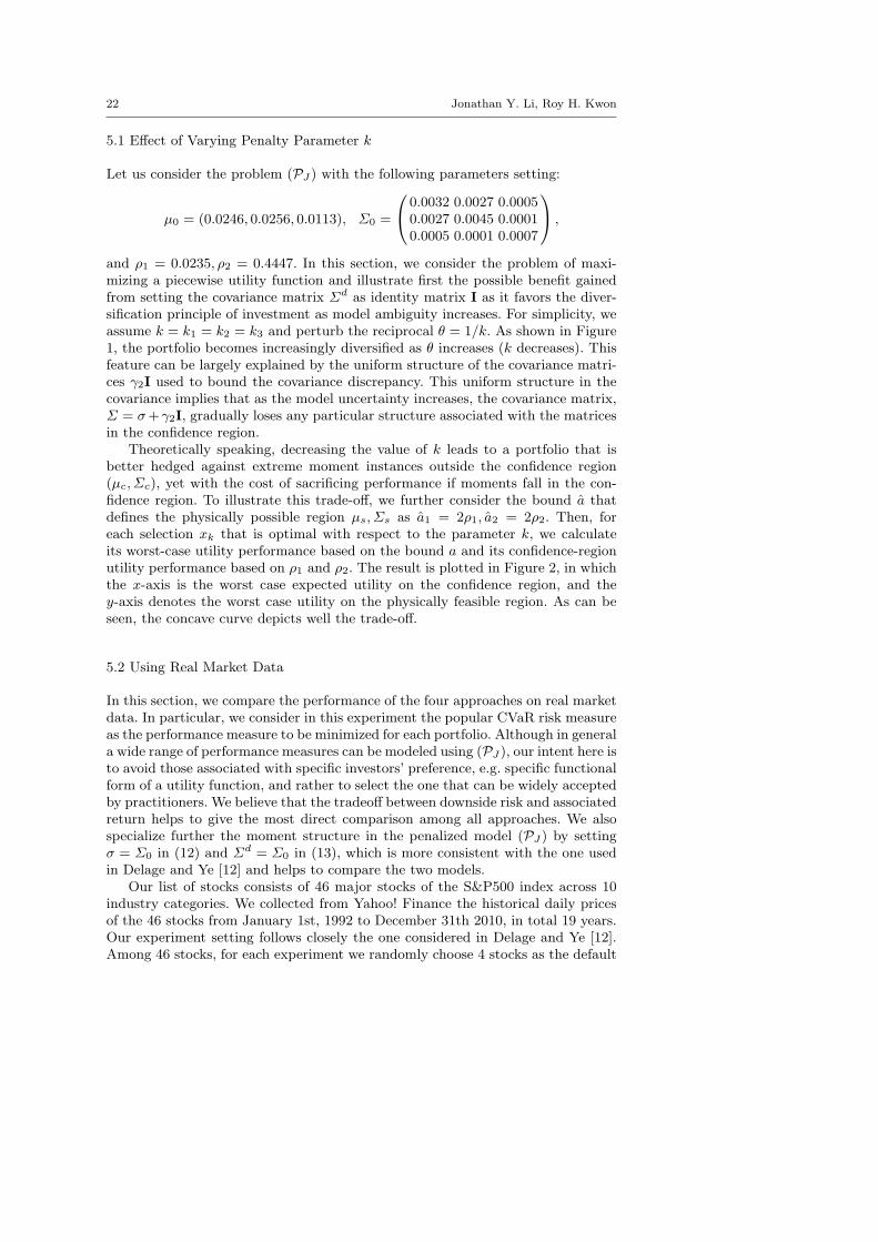
5.1 Effect of Varying Penalty Parameter k
Let us consider the problem (PJ) with the following parameters setting:
µ0 = (0.0246, 0.0256, 0.0113), Σ0 =
0.0032 0.0027 0.00050.0027 0.0045 0.00010.0005 0.0001 0.0007
,
and ρ1 = 0.0235, ρ2 = 0.4447. In this section, we consider the problem of maxi-mizing a piecewise utility function and illustrate first the possible benefit gainedfrom setting the covariance matrix Σd as identity matrix I as it favors the diver-sification principle of investment as model ambiguity increases. For simplicity, weassume k = k1 = k2 = k3 and perturb the reciprocal θ = 1/k. As shown in Figure1, the portfolio becomes increasingly diversified as θ increases (k decreases). Thisfeature can be largely explained by the uniform structure of the covariance matri-ces γ2I used to bound the covariance discrepancy. This uniform structure in thecovariance implies that as the model uncertainty increases, the covariance matrix,Σ = σ+γ2I, gradually loses any particular structure associated with the matricesin the confidence region.
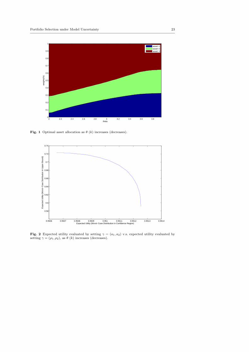
Theoretically speaking, decreasing the value of k leads to a portfolio that isbetter hedged against extreme moment instances outside the confidence region(µc, Σc), yet with the cost of sacrificing performance if moments fall in the con-fidence region. To illustrate this trade-off, we further consider the bound a thatdefines the physically possible region µs, Σs as a1 = 2ρ1, a2 = 2ρ2. Then, foreach selection xk that is optimal with respect to the parameter k, we calculateits worst-case utility performance based on the bound a and its confidence-regionutility performance based on ρ1 and ρ2. The result is plotted in Figure 2, in whichthe x-axis is the worst case expected utility on the confidence region, and they-axis denotes the worst case utility on the physically feasible region. As can beseen, the concave curve depicts well the trade-off.
5.2 Using Real Market Data
In this section, we compare the performance of the four approaches on real marketdata. In particular, we consider in this experiment the popular CVaR risk measureas the performance measure to be minimized for each portfolio. Although in generala wide range of performance measures can be modeled using (PJ), our intent here isto avoid those associated with specific investors’ preference, e.g. specific functionalform of a utility function, and rather to select the one that can be widely acceptedby practitioners. We believe that the tradeoff between downside risk and associatedreturn helps to give the most direct comparison among all approaches. We alsospecialize further the moment structure in the penalized model (PJ) by settingσ = Σ0 in (12) and Σd = Σ0 in (13), which is more consistent with the one usedin Delage and Ye [12] and helps to compare the two models.
Our list of stocks consists of 46 major stocks of the S&P500 index across 10industry categories. We collected from Yahoo! Finance the historical daily pricesof the 46 stocks from January 1st, 1992 to December 31th 2010, in total 19 years.Our experiment setting follows closely the one considered in Delage and Ye [12].Among 46 stocks, for each experiment we randomly choose 4 stocks as the default
Portfolio Selection under Model Uncertainty 23
2 2.2 2.4 2.6 2.8 3 3.2 3.4 3.6 3.80
0.1
0.2
0.3
0.4
0.5
0.6
0.7
0.8
0.9
1
theta
wei
ghts
(%)
asset−1asset−2asset−3
Fig. 1 Optimal asset allocation as θ (k) increases (decreases).
0.9506 0.9507 0.9508 0.9509 0.951 0.9511 0.9512 0.9513 0.9514
0.58
0.6
0.62
0.64
0.66
0.68
0.7
0.72
0.74
Expected Utility (Worst−Case Distribution in Confidence Region)
Exp
ecte
d U
tility
(W
orst
−C
ase
Dis
trib
utio
n in
Upp
er B
ound
)
Fig. 2 Expected utility evaluated by setting γ = (a1, a2) v.s. expected utility evaluated bysetting γ = (ρ1, ρ2), as θ (k) increases (decreases).
24 Jonathan Y. Li, Roy H. Kwon
portfolio and then rebalance the portfolio every 15 days. At each time of con-structing/rebalancing a portfolio, the prior 30-days daily data is used to estimatesampled mean and covariance. As Delage and Ye has shown that their approachoutperforms other approaches under such a setting, our hope is to carry over theirhigh quality result to this experiment and compare it with our penalized approach.Our choice of time period to examine the performance of each approach is inspiredby the choices in Goldfarb and Iyengar [16], where the time period January 1997– December 2000 is chosen, and in Delage and Ye [12], where the time period2001 – 2007 is chosen. To further cover the most recent financial crisis, the entiretime period that we consider to evaluate the performance is from January 1997 toDecember 2010. The dataset for the time period January 1992 – December 1996was used for initial parameter estimation.
We assume in this experiment that investors hold strictly conservative attitudesand pursue only robust performance when the moments are realized within 90%confidence region. To estimate the parameters ρ1 and ρ2 that correspond to the90% confidence region, we apply similar statistical analysis as the one used inDelage and Ye [12]. It is however difficult to determine the “right” amount ofdata that gives the “best” estimation of ρ1 and ρ2. To mitigate possible bias dueto the choice of the amount of data, in addition to the initial estimation basedon the data from January 1992 to December 1996 another re-estimation basedon the data from January 1992 to December 2003 is further performed in themiddle of the rebalancing period, i.e. January 2004. Thus, in our later analysisthe portfolio performance of the first 7-years period (1997-2003) will be presentedseparately from the latter 7-years period (2004-2010). The estimation of ρ1 andρ2 with respect to the 90% confidence region are given as follows
ρ1−90% = 0.1816, ρ2−90% = 3.7356, (1992− 1996)
ρ1−90% = 0.1860, ρ2−90% = 4.3827, (1992− 2003).
In addition to parameters ρ1 and ρ2, penalty parameters k1, k2, k3 are alsorequired to be estimated for our model (PJ). Various approaches may be consid-ered to estimate the penalty parameters. For example, one may attempt to findthose values which generally lead to superior portfolio performance by solving(PJ) repeatedly based on some historical data. However, this additional calibra-tion procedure, which may (or may not) give unfair advantages over classical DROapproaches, may hinder us to provide a consistent comparison and weaken the il-lustration of the benefit accrued solely from the bounds that are endogenouslygenerated from our penalized approach. As an alternative approach, in this ex-periment we generate the penalty parameters by the following procedure. At thetime that we estimate ρ1−90% and ρ2−90%, we additionally estimate another setof parameters ρ1−99% and ρ2−99% that corresponds to a 99%-confidence region:
ρ1−99% = 0.3779, ρ2−99% = 9.3773 (1992− 1996)
ρ1−99% = 0.4161, ρ2−99% = 12.1698 (1992− 2003).
We assume that the penalty parameters are calibrated in a way that the optimalportfolio generated by model (PJ) with a 90% confidence region is identical to theone generated by Delage and Ye’s model with a 99% confidence region at the timeof parameter estimation. Following Remark 4, we can compute the value of the

Portfolio Selection under Model Uncertainty 25
penalty parameters by solving (PJ), where the difference a1 = ρ1−99% − ρ1−90%
and a2 = ρ2−99%−ρ2−90% is set as the upper bound of γ1, γ2 and k1 = k2 = k3 = 0.This overall estimation procedure will help compare fairly the following three mod-els: Delage and Ye’s model with parameters ρ = (ρ1−90%, ρ2−90%) (denoted byDY-90), with parameters ρ = (ρ1−99%, ρ2−99%) (denoted by DY-99), and our pe-nalized model (PJ) with parameters ρ = (ρ1−90%, ρ2−90%) and penalty parametersestimated by a1, a2 (denoted by LK-90). Note that as the sampled mean and co-variance are re-estimated at each rebalancing point, DY-90 and DY-99 have ρ1, ρ2unchanged; that is, the fixed bounds remain the same while LK-90 instead keepsits penalty parameters unchanged.
In addition to the above three models, the performance of Popescu’ model (de-noted by P), and a sample-based approach (denoted by SB) will also be compared.The comparison in terms of average (avg.), geometric mean (geo.) and CVaR mea-sures of various quantiles δ among all models for the time periods 1997-2003 and2004-2010 are given in Table 1 and Table 2. Various CVaR measures are providedto ensure the consistency of the performance in terms of downside risk. As theeconomy has experienced a dramatic change before and after the 2008 financialcrisis, we further provide the comparison for the time periods 2004-2007 and 2007-2010, which are separately given in Table 3 and Table 4. As shown in the tables,among 300 experiments LK-90 exhibits overall superior performance among allthe models except having lower mean and geometric mean than the P and the SPmodel during 2004-2007. For that time period, it appears that even though theP and the SP model still expose to higher downside risk than other approaches,they enjoy the most advantage of upward trend of the market and achieve bet-ter average return. One possible reason for this is that the market for the timeperiod 2004-2007 is less volatile (compared with other time periods), for whicha sample-based approach can possibly benefit the most from using only sampledata. On the other hand, in all other time periods Delage and Ye’s and our penal-ized approach not only perform better than the P and the SP approach in termsof CVaR values, where the improvement can go up to 5∼10% for δ = 1, but alsoachieve superior average performance, where the improvement can go up to around0.3%. This overall superior performance is also carried over to the comparison oflong-term performance; for example, the average yearly return is also improved upto 3∼10% by using Delage and Ye’s model or our penalized model. This verifiesthe importance of taking moment uncertainty into account in real-life portfolioselection, which helps to achieve more efficient portfolios.
Table 1 Comparison of different approaches in the period: 1997/01-2003/12
avg. geo. δ = 0.01 δ = 0.1 δ = 1 δ = 5 δ = 10 yr. ret.P 1.0043 1.0014 0.4375 0.6631 0.7553 0.8321 0.8662 1.0685
DY-90 1.0062 1.0046 0.6931 0.733 0.7986 0.8721 0.9000 1.0931DY-99 1.007 1.0053 0.6908 0.7328 0.8002 0.8752 0.9027 1.1042LK-90 1.0073 1.0056 0.6911 0.7328 0.8005 0.8762 0.9036 1.1087
SP 1.0043 1.0008 0.4375 0.5577 0.7301 0.8168 0.8535 1.0703
By comparing the performance of DY-90, DY-99 and LK-90, we can first seethat LK-90 has a clear advantage over DY-90. Since DY-99 also outperforms DY-90, this verifies the intuition that if there is any additional gain by increasing the

26 Jonathan Y. Li, Roy H. Kwon
Table 2 Comparison of different approaches in the period: 2004/01-2010/12
avg. geo. δ = 0.01 δ = 0.1 δ = 1 δ = 5 δ = 10 yr. ret.P 1.0042 1.0018 0.5634 0.5799 0.7233 0.8297 0.8723 1.0597
DY-90 1.004 1.0027 0.6219 0.6835 0.7717 0.8676 0.9046 1.0642DY-99 1.0044 1.0032 0.6314 0.6878 0.7772 0.8739 0.9098 1.0718LK-90 1.0047 1.0036 0.6417 0.6918 0.7803 0.8763 0.9115 1.0772
SP 1.0043 1.0013 0.5634 0.5786 0.6992 0.8158 0.8605 1.0599
Table 3 Comparison of different approaches in the period: 2004/01-2007/06
avg. geo. δ = 0.01 δ = 0.1 δ = 1 δ = 5 δ = 10 yr. ret.P 1.0091 1.0081 0.8142 0.8411 0.8686 0.9101 0.9292 1.0597
DY-90 1.0074 1.0069 0.8784 0.8955 0.92 0.9421 0.9529 1.0642DY-99 1.0073 1.0069 0.8743 0.8955 0.9246 0.9459 0.956 1.0718LK-90 1.0073 1.0069 0.8737 0.8963 0.9251 0.9461 0.956 1.0772
SP 1.0095 1.0083 0.782 0.8245 0.861 0.9019 0.9218 1.0599
Table 4 Comparison of different approaches in the period: 2007/06-2010/12
avg. geo. δ = 0.01 δ = 0.1 δ = 1 δ = 5 δ = 10 yr. ret.P 0.9994 0.9957 0.5634 0.5634 0.6776 0.7847 0.8334 0.901
DY-90 1.0008 0.9987 0.6142 0.6675 0.7366 0.8265 0.8689 0.9545DY-99 1.0016 0.9996 0.6253 0.674 0.7429 0.8325 0.8752 0.9716LK-90 1.0022 1.0003 0.6199 0.677 0.7479 0.8357 0.8776 0.9826
SP 0.9991 0.9946 0.5634 0.5634 0.6563 0.7671 0.819 0.887
fixed bound of the confidence region, our penalized approach can as well effectivelybenefit from such a gain. To explain the reason why DY-99 outperforms DY-90 is not easy as we have discussed earlier that deciding appropriate bounds ishighly non-trivial. What can however be intriguing is that in most cases LK-90outperforms DY-99 in terms of both average return and downside risk performance.Although the improvement is not as substantial as it is on other models, whichis actually plausible as we enforce the consistency of the initial setting betweenDY-99 and LK-90, we believe that this overall superior performance does reflectthe benefit from using a penalized approach, which endogenously determines thebound at each rebalancing point according to the level of deterioration in worst-case performance. Furthermore, as shown in Table 2, the improvement of the CVaRvalue can still go up to 1.5% while the improvement of average return is 0.03%.Another important observation is that in the time period 2007-2010, where themarket is most volatile, the improvement of LK-90 over DY-99 is most substantialin terms of average return, and the improvement of average yearly return is asmuch as the improvement of DY-99 over DY-90. By contrasting the improvementof LK-90 over DY-99 between the time periods 2004-2007 and 2007-2010, we findthat the more volatile the market is, the more one can possibly benefit from usingour penalized approach.
In Figure 3 - 6 we have also provided the average evolution of cumulative wealthfor each model for time periods 1997-2003, 2004-2010, 2004-2007, and 2007-2010.Note that in all figures the evolution of a unit price of the S&P500 index hasalso been provided for reference purpose. As seen, for the time period 1997-2003,the P and the SP model show their vulnerability in a constantly volatile marketand their associated cumulative wealth dropped greatly as the market crashed
Portfolio Selection under Model Uncertainty 27
around 2001-2002, whereas DY-90, DY-99 and LK-90 have much better downsiderisk performance. One can also observe the strength of the penalized model LK-90compared with DY-90 and DY-99: its greater wealth is cumulated by consistentlyproviding more stable performance in a volatile market. Similar observation canalso be found in the time period 2004-2010. This comparison contrasts further a“fixed-bound” approach with our “endogenous bound” approach. The overall com-putational results support well the idea that the penalized problem (PJ) whichendogenously decides the bound of moments based on the level of deteriorationin worst-case performance, improves the overall performance. In addition, the his-togram of terminal wealth for each model provided in Figure 7, 8, 9 and 10 alsofurther verifies the overall superior long-term performance of LK-90.
6 Conclusion and Future Work
In this paper, we consider a single-period portfolio selection problem and addressthe difficulty of providing a “reasonably” robust policy in the presence of a par-ticular type of model ambiguity: moment uncertainty. We propose a penalizedmoment-based framework that integrates the classical DRO approaches with theidea of comprehensive robust optimization. While the classical DRO approachesfocus on ensuring the solution is robust against a bounded set of moment vec-tors, our integrated approach provides additional level of robustness when therealized moments fall outside the set. Under some mild conditions, the penalizedmoment-based problem turns out to be computationally tractable for a wide rangeof specifications. Computational experiments were conducted, where we specializethe penalized problem to the portfolio selection model in Delage and Ye [12] andfind promising performance of our approach using historical data. In most cases,our penalized moment-based approach achieves better performance in terms ofthe average return and CVaR downside risk measure. We also find that the im-provement of performance becomes more substantial as the market becomes morevolatile. This highlights the potential benefit of endogenously achieving bounds formoment uncertainty using our penalized approach. We have also provided a fewpractical extensions of the problem. The practical performance of those extensionsremains to be examined, and we will leave those examinations for our future work.
A Appendix
A.1 Connection with KL-divergence
Consider KL-divergence of two multivariate normal distributions N (µ,Σ), N0(µ0, Σ0) whichcan be calculated as follows. Note that Kullback-Leibler (KL) divergence is the quantity thata relative entropy function measures the discrepancy between two distributions (see, e.g. Kull-back [21] and Kullback and Leibler [22])
DKL(N||N0) :=1
2( loge(
detΣ0
detΣ) +Σ−1
0 •Σ + (µ− µ0)TΣ−1
0 (µ− µ0)−N ).
The formula indicates that under an ellipsoidal norm scaled by Σ−10 the discrepancy between
two mean vectors directly implies the magnitude of KL-divergence. Next, for a fixed Σ0, byderiving the derivative of the function DKL(N||N0) along the direction ∆Σ at any given Σ, one

28 Jonathan Y. Li, Roy H. Kwon
can find DDKL(N||N0)[∆Σ] = 12( ∆Σ • (Σ−1
0 − Σ−1) ).3 This implies that the discrepancy ofcovariance eigenvalues is positively correlated with the magnitude of KL-divergence. Hence, inthe case of normal distribution, the preference order given according to moment discrepancycoincides with the order given according to distribution discrepancy measured in terms ofKL-divergence.
A.2 Proofs
A.2.1 Proof of Lemma 1:
Given that dµ (resp. dΣ) is a convex function, by definition the epigraph Sµ := {(µ, t) | dµ(µ, µc) ≤t} (resp. SΣ := {(Σ, s) | dΣ(Σ,Σc) ≤ s}) is a convex set. Since (µα, αµ), (µβ , βµ) ∈ Sµ and(Σα, αΣ), (Σβ , βΣ) ∈ SΣ , the following holds for any 0 ≤ λ1 ≤ 1, 0 ≤ λ2 ≤ 1 according to theproperty of a convex set
λ1(µα, αµ) + (1− λ1)(µβ , βµ) ∈ Sµ
λ2(Σα, αΣ) + (1− λ2)(Σβ , βΣ) ∈ SΣ .
Thus, given that
(ηµηΣ
)= λ
(αµ
αΣ
)+ (1− λ)
(βµ
βΣ
)and 0 ≤ λ ≤ 1, the above implies that
∃µη , Ση such that µη = λµα + (1− λ)µβ and Ση = λΣα + (1− λ)Σβ also satisfy
dµ(µη , µc) ≤ ηµ, dΣ(Ση , Σc) ≤ ηΣ
by setting λ1 = λ2 = λ. Finally, it is trivial to see that the probability measure λQα+(1−λ)Qβ
indeed satisfies
EλQα+(1−λ)Qβ[X] = λEQα [X] + (1− λ)EQβ
[X],
where X is a random variable. This completes the proof. �
A.2.2 Proof of Theorem 1:
It suffices to show that for a fixed x the function F(x, γ) in (7) is concave with respect to γ dueto induced concavity of −rk(γ). Let us consider the functional λF(x, γα) + (1 − λ)F(x, γβ).Let
Q′α(β) := arg max
Q∈{Q(· ; µ,Σ) : dµ,dΣ≤γα(β)}
∫G(wT x)dQ(w),
where we abbreviate the notation dµ(µ, µc) and dΣ(Σ,Σc) as dµ dΣ . Then,
λF(x, γα) + (1− λ)F(x, γβ) =
∫G(wT x)d(λQ′
α + (1− λ)Q′β)(w). (19)
Lemma 1 gives us that there exists Q′η ∈ {Q(· ; µ,Σ) : dµ, dΣ ≤ λγα + (1− λ)γβ} such that
Q′η = λQ′
α + (1− λ)Q′β .
Suppose that Q′′η = argmaxQ∈{Q(· ; µ,Σ) : dµ,dΣ≤λγα+(1−λ)γβ}
∫G(wT x)dQ(w). It follows
that
(19) =
∫G(wT x)dQ′
η(w) ≤∫
G(wT x)dQ′′η (w) = F(x, λγα + (1− λ)γβ).
This shows the concavity of F(x, γ) with respect to γ. �
3 Df(x)[∆x] denotes the derivative of a mapping f : ℜn → ℜm at a point x.
Portfolio Selection under Model Uncertainty 29
A.2.3 Proof of Theorem 4:
To show that γki is monotonically decreasing as ki increases, it suffices to discuss the case ofincreasing a univariate kij . Suppose that k1j and k2j are fixed such that k1j < k2j . Let γk1 be the
optimal γ w.r.t. k1j and γk2 be the optimal γ w.r.t. k2j . By definition, the following inequalities
hold
F(x, γk1 )− k1j · rj(γk1 ) ≥ F(x, γk2 )− k1j · rj(γk2 )
F(x, γk2 )− k2j · rj(γk2 ) ≥ F(x, γk1 )− k2j · rj(γk1 ).
By adding the first inequality to the second inequality, we obtain (k1j −k2j )(rj(γk2 )−rj(γk1 )) ≥0. k1j < k2j implies that rj(γk1 ) ≥ rj(γk2 ). Since rj(γ) ≥ 0 and that rj(γ) is non-decreasing,
we attain γk2 ≤ γk1 . For the case of two vectors k1 < k2 one can increase each entry of k1 ata time and finally attain k2. Since at each step γ is monotonically decreasing, γk2 ≤ γk1 stillholds for k1 < k2. This also implies that F(x, γk2 ) ≤ F(x, γk1 ) for a fixed x.
Now, consider the relation between F(xk1 , γk1 ) and F(xk2 , γk2 ), where xk1 and xk2 arerespective optimal solutions with respect to k1 and k2. Based on the above result, the inequalityF(xk1 , γk2 ) ≤ F(xk1 , γk1 ) holds. In addition, since xk2 is the minimizer with respect to k2,the inequality F(xk2 , γk2 ) ≤ F(xk1 , γk2 ) must hold as well. Then, these two inequalities implythat F(xk2 , γk2 ) ≤ F(xk1 , γk1 ) �
A.2.4 Proof of Theorem 5:
It suffices to prove that for a fixed x, if γ∗ is an optimal solution for the inner optimizationproblem of the first problem with parameter k∗, there exists a b∗ for the second problem suchthat γ∗ is also optimal for its inner optimization problem given x. Based on the optimalitycondition of convex optimization problems (see, e.g. Bertsekas [6]), for γ∗ to be an optimalsolution of the first problem it is required that
F(x, γ∗)−I∑
i=1
kiri(γ∗)−
∑j
λj(γ∗j − aj) ≥ F(x, γ)−
I∑i=1
kiri(γ)−∑j
λj(γj − aj),∀γ,
and λj(γ∗j − aj) = 0, λj ≥ 0. Similarly, for γ∗ to be an optimal solution of the second problem,
it is required that
F(x, γ∗)−I∑
i=1
ρi(ri(γ∗)−bi)−
∑j
vj(γ∗j −aj) ≥ F(x, γ)−
I∑i=1
ρi(ri(γ)−bi)−∑j
vj(γj−aj),∀γ,
and ρi(ri(γ∗)− bi) = 0, vj(γ
∗j − aj) = 0, ρi, vj ≥ 0. This optimality condition is equivalent to
F(x, γ∗)−I∑
i=1
ρiri(γ∗)−
∑j
vj(γ∗j − aj) ≥ F(x, γ)−
I∑i=1
ρiri(γ)−∑j
vj(γj − aj),∀γ,
and ρi(ri(γ∗) − bi) = 0, vj(γ
∗j − aj) = 0, ρi, vj ≥ 0. Then, if γ∗, λj is a solution of the first
system, γ∗, λj is also a solution for the second system with bi = ri(γ∗), vj = λj , and ρi = ki.
For the other direction, if γ∗, ρi, vj is a solution for the second system, then γ∗, ρi, vj is alsoa solution for the first system with ki = ρi, λj = vj . �
Acknowledgements The authors gratefully acknowledge Natural Sciences and EngineeringResearch Council of Canada (NSERC) for financial support of this research and Michael J.Kim for valuable discussions to improve the initial draft.

30 Jonathan Y. Li, Roy H. Kwon
References
1. Anderson, E. W., Hansen L. P., Sargent T. J.: Robustness, detection and the price of risk.(2000)
2. Ben-Tal, A., Bertsimas D., Brown D. B.: A soft robust model for optimization under am-biguity. Oper. Res. 58(4), 1220–1234 (2010)
3. Ben-Tal, A., Nemirovski A.: Lectures on Modern Convex Optimization: Analysis, Algo-rithms, and Engineering Applications, MPS/SIAM Series on Optimization. SIAM, Philadel-phia, PA. (2001)
4. Ben-Tal, A., Nemirovski A.: Robust optimization - methodology and applications. Math.Program., Ser. B 92(3), 453–480 (2002)
5. Ben-Tal, A., Boyd S., Nemirovski A.: Extending scope of robust optimization: compre-hensive robust counterparts of uncertain problems. Math. Program., Ser. B 107(1), 63–89(2006)
6. Bertsekas, D.: Nonlinear Programming, 2nd ed. Athena Scientific, Belmont, MA. (1999)7. Bertsimas, D., Sim M.: The price of robustness. Oper. Res. 52(1), 35–53 (2004)8. Black, F., Litterman R.: Global portfolio optimization. Finan. Anal. J., 28–43 (1992)9. Calafiore G.: Ambiguous risk measures and optimal robust portfolios. SIAM J. Optim.18(3), 853–877 (2007)
10. Chen, W., Sim M.: Goal-driven optimization. Oper. Res. 57(2), 342–357 (2009)11. Cont R.: Model uncertainty and its impact on the pricing of derivative instruments. Math.Finan. 16, 519–547 (2006)
12. Delage, E., Ye Y.: Distributionally robust optimization under moment uncertainty withapplication to data-driven problems. Oper. Res. 58(3), 595–612 (2010)
13. El Ghaoui, L., Oks M., Oustry. F.: Worst-case value-at-risk and robust portfolio optimiza-tion: a conic programming approach. Oper. Res. 51(3), 543–556 (2003)
14. Ellsberg, D.: Risk, ambiguity, and the savage axioms. Quart. J. Econ. 75(4), 643–669(1961)
15. Gilboa, I., Schmeidler D.: Maxmin expected utility with a non-unique prior. J. Math.Econ. 18(2), 141–153 (1989)
16. Goldfarb, D., Iyengar G.: Robust portfolio selection problems. Math. Oper. Res. 28(1),1–38 (2003)
17. Goldfarb, D., Scheinberg, K.: On parametric semidefinite programming. Appl. Numer.Math. 29(3), 361–377 (1999)
18. Grotschel, M., Lovasz L., Schrijver A.: The ellipsoid method and its consequences incombinatorial optimization. Combinatorica 1(2), 169–197 (1981)
19. Hansen, L., Sargent T.: Robust control and model uncertainty. Amer. Econ. Rev. 91(2),60–66 (2001)
20. Kolda, T. G., Lewis R. M., Torczon V.: Optimization by direct search: new perspectiveson some classical and modern methods. SIAM Rev. 45(3), 385–482 (2003)
21. Kullback, S.: Information Theory and Statistics. John Wiley and Sons, New York (1959)22. Kullback, S., Leibler R. A.: On information and sufficiency. Ann. Math. Statist. 22(1),79–86 (1951)
23. Luenberger D. G.: Investment Science. Oxford University Press, Oxford, U.K. (1999)24. Maenhout P. J.: Robust portfolio rules and asset pricing. Rev. Finan. Stud. 17(4), 951–983(2004)
25. Natarajan, K., Pachamanova D., Sim M.: Incorporating asymmetric distributional infor-mation in robust value-at-risk optimization. Manage. Sci. 54(3), 573–585 (2008)
26. Natarajan, K., Sim M., Uichanco J.: Tractable robust expected utility and risk models forporfolio optimization. Math. Finan. 20(4), 695-731.
27. Nesterov, Y., Nemirovski A.: Interior Point Polynomial Methods in Convex Programming:Theory and Applications. SIAM, Philadelphia, PA. (1994)
28. Popescu, I.: Robust mean-covariance solutions for stochastic optimization. Oper. Res.55(1), 98–112 (2007)
29. Shapiro, A.: On duality theory of conic linear problems. In: Goberna, M. A., Lopez M. A.(eds.) Semi-Infinite Programming: Recent Advances, pp. 135–165. Kluwer Academic Pub-lishers (2001)
30. Tutuncu R. H., Koenig M.: Robust asset allocation. Ann. Oper. Res. 132, 157–187 (2004)31. Uppal, R., Wang T.: Model misspecification and under-diversification. J. Finan. 58(6),2465–2486 (2003)
32. Vandenberghe, L., Boyd. S.: Semidefinite programming. SIAM Rev. 38(1), 49–95 (1996)

Portfolio Selection under Model Uncertainty 31
33. Wolkowicz, H., Saigal R., Vandenberghe L., eds: Handbook of Semidefinite Programmingand Applications. Kluwer Academic Publishers (2000)
34. Zhu, S. S., Fukushima M.: Worst-case conditional value-at-risk with application to robustportfolio management. Oper. Res. 57(5), 1155–1168 (2009)

32 Jonathan Y. Li, Roy H. Kwon
0 20 40 60 80 100 120
1
1.2
1.4
1.6
1.8
2
2.2
15 days/unit
Cum
ulat
ive
Wea
lth (
$)Jan. 1997 − Dec. 2003
PDY−90DY−99LK−90SPS&P500
Fig. 3 Cumulative wealth for the time period: 1997/01-2003/12.
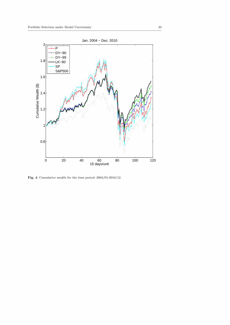
Portfolio Selection under Model Uncertainty 33
0 20 40 60 80 100 120
0.8
1
1.2
1.4
1.6
1.8
2
15 days/unit
Cum
ulat
ive
Wea
lth (
$)Jan. 2004 − Dec. 2010
PDY−90DY−99LK−90SPS&P500
Fig. 4 Cumulative wealth for the time period: 2004/01-2010/12.
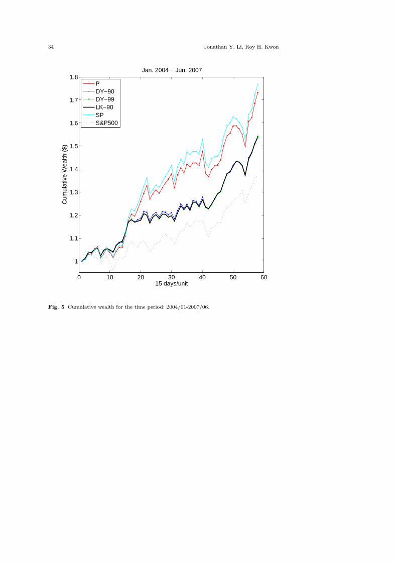
34 Jonathan Y. Li, Roy H. Kwon
0 10 20 30 40 50 60
1
1.1
1.2
1.3
1.4
1.5
1.6
1.7
1.8
15 days/unit
Cum
ulat
ive
Wea
lth (
$)Jan. 2004 − Jun. 2007
PDY−90DY−99LK−90SPS&P500
Fig. 5 Cumulative wealth for the time period: 2004/01-2007/06.
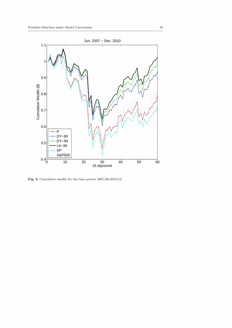
Portfolio Selection under Model Uncertainty 35
0 10 20 30 40 50 600.4
0.5
0.6
0.7
0.8
0.9
1
1.1
15 days/unit
Cum
ulat
ive
Wea
lth (
$)Jun. 2007 − Dec. 2010
PDY−90DY−99LK−90SPS&P500
Fig. 6 Cumulative wealth for the time period: 2007/06-2010/12.

36 Jonathan Y. Li, Roy H. Kwon
0 1 2 3 4 5 6 70
20
40
60
80
100
120
140
Cumulative Wealth ($)
Fre
quen
cy
Histogram of Jan. 1997 − Dec. 2003
PDY−90DY−99LK−90SP
Fig. 7 Histogram of terminal wealth for all approaches in the period 1997/01-2003/12.
0 1 2 3 4 50
20
40
60
80
100
120
140
160
180
Cumulative Wealth ($)
Fre
quen
cy
Histogram of Jan. 2004 − Dec. 2010
PDY−90DY−99LK−90SP
Fig. 8 Histogram of terminal wealth for all approaches in the period 2004/01-2010/12.
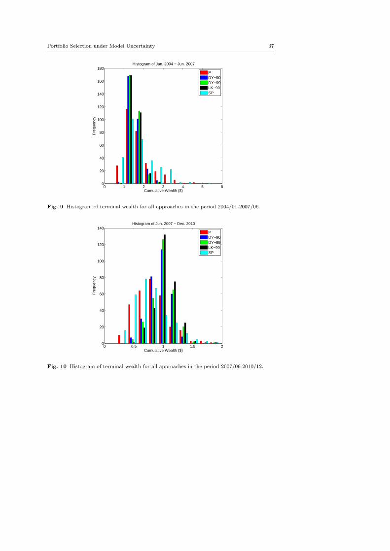
Portfolio Selection under Model Uncertainty 37
0 1 2 3 4 5 60
20
40
60
80
100
120
140
160
180
Cumulative Wealth ($)
Fre
quen
cy
Histogram of Jan. 2004 − Jun. 2007
PDY−90DY−99LK−90SP
Fig. 9 Histogram of terminal wealth for all approaches in the period 2004/01-2007/06.
0 0.5 1 1.5 20
20
40
60
80
100
120
140
Cumulative Wealth ($)
Fre
quen
cy
Histogram of Jun. 2007 − Dec. 2010
PDY−90DY−99LK−90SP
Fig. 10 Histogram of terminal wealth for all approaches in the period 2007/06-2010/12.