portfolio selection with higher moments - duke's fuqua ...charvey/research/... · portfolio...

Portfolio Selection with Higher Moments | 589

Campbell R. Harvey, John C. Liechty, Merrill W. Liechty, and Peter Müller, “Portfolio Selection With Higher Moments,” pp. 1–41. Copyright © Campbell R. Harvey. Permission to reprint granted by the author.

Portfolio Selection with Higher Moments

By Campbell R. Harvey, John C. Liechty, Merrill W. Liechty, and Peter Müller*

ABSTRACT

We propose a method for optimal portfolio selection using a Bayesian decision theoretic framework that addresses two major shortcom-ings of the Markowitz approach: the ability to handle higher moments and estimation error. We employ the skew normal distribution which has many attractive features for modeling mul-tivariate returns. Our results suggest that it is important to incorporate higher order moments in portfolio selection. Further, our comparison to other methods where parameter uncertainty is either ignored or accommodated in an ad hoc way, shows that our approach leads to higher expected utility than the resampling methods that are common in the practice of fi nance.

Keywords: Bayesian decision problem, multivariate skew-ness, parameter uncertainty, optimal portfolios, utility function maximization.

* Campbell R. Harvery is J. Paul Sticht Professor of International Business, Fuqua School of Business, Duke University, Durham NC 27708 and Research Associate, National Bureau of Economic Research, Cambridge, MA 02138 (E-mail: [email protected]). John C. Liechty is Assistant Professor, Department of Marketing, Smeal College of Business, and Department of Statistics, Pennsylvania State University, University Park, PA 16803 (E-mail: [email protected]). Merrill W. Liechty is Assistant Professor, Department of Decision Sciences, LeBow College of Business, Drexel University, Philadelphia, PA 19104 (E-mail: [email protected]). Peter Müller is Professor, Department of Biostatistics, Th e University of Texas M. D. Anderson Cancer Center, Houston, TX 77030 (E-mail: [email protected]). We appreciate the comments of Philippe Jorion, Harry Markowitz, Haim Lévy, Michael Brandt, Chris Adcock and Karl Shutes.

1. INTRODUCTION

M arkowitz (1952a) provides the foundation for the current theory of asset allocation. He describes the task of asset “allocation as

having two stages. Th e fi rst stage “starts with observation and experience and ends with beliefs about the future performances of available securities.” Th e second stage “starts with the relevant beliefs … and ends with the selec-tion of a portfolio.” Although Markowitz only deals with the second stage, he suggests that the fi rst stage should be based on a “probabilistic” model. However, in the usual implementation of Markowitz’s second stage, we are as-sumed to know with certainty the inputs from the fi rst stage, i.e. the exact means, variances and covariances. Th is paper introduces a method for addressing both stages.

In a less well known part of Markowitz (1952a, p.91), he details a condition whereby mean-variance effi cient portfolios will not be optimal—when an investor’s util-ity is a function of mean, variance, and skewness. While Markowitz did not work out the optimal portfolio selection in the presence of skewness and other higher moments, we do. We develop a framework for optimal portfolio selection in the presence of higher order moments and parameter uncertainty.

Several authors have proposed advances to optimal portfolio selection methods. Some address the empirical evidence of higher moments; Athayde and Flôres (2003, 2004) and Adcock (2002) give methods for determining higher dimensional ‘effi cient frontiers’, but they remain in the certainty equivalence framework (assuming exact knowledge of the inputs) for selecting an optimal portfolio. Like the standard effi cient frontier approach, these ap-proaches have the advantage that for a large class of utility functions, the task of selecting an optimal portfolio reduces to the task of selecting a point on the high dimensional ‘effi cient frontiers’. Other three moment optimization

590 | Applied Financial Economics

methods include using negative semi-variance in place of variance (see Markowitz 1959 and Markowitz, Todd, Xu, and Yamane 1993). A similar measure of downside risk is incorporated by Feiring, Wong, Poon, and Chan (1994), and Konno, Shirakawa, and Yamazaki (1993) who use an approximation to the lower semi-third moment in their Mean-Absolute Deviation-Skewness portfolio model. Th ese methods rest on the assumption that an investor’s expected utility is reasonably approximated by inserting estimates of the moments of an assumed sampling model.

A number of researchers have shown that mean-vari-ance effi cient portfolios, based on estimates and ignoring parameter uncertainty, are highly sensitive to perturbations of these estimates. Jobson, Korkie and Ratti (1979) and Jobson and Korkie (1980) detail these problems and suggest the use of shrinkage estimators. Th is ‘estimation risk’ comes from both choosing poor probability models and from ignoring parameter uncertainty, maintaining the assumption that expected utility can be evaluated by substituting point estimates of sampling moments in the utility function.

Others have ignored higher moments, but address the issue of estimation risk. Frost and Savarino (1986, 1988) show that constraining portfolio weights, by restricting the action space during the optimization, reduces estimation error. Jorion (1992) proposes a resampling method aimed at estimation error. Using a Bayesian approach, Britten-Jones (2002) proposes placing informative prior densities directly on the portfolio weights. Others propose methods that address both stages of the allocation task and select a portfolio that optimizes an expected utility function given a probability model. From the Bayesian perspective, Jorion (1986) use a shrinkage approach while Treynor and Black (1973) advocate the use of investors’ views in combina-tion with historical data. Kandel and Stambaugh (1996) examine predictability of stock returns when allocating between stocks and cash by a risk-averse Bayesian investor. (See also Johannes, Polson, and Stroud 2002 who examine the market timing relationship to performance of optimal portfolios using a model with correlation between volatil-ity and returns in a Bayesian portfolio selection setting.) Zellner and Chetty (1965), Klein and Bawa (1976) and Brown (1978) emphasize using a predictive probability model (highlighting that an investor’s utility should be given in terms of future returns and not parameters from a sampling distribution). Pástor and Stambaugh (2000) study the implications of diff erent pricing models on

optimal portfolios, updating prior beliefs based on sample evidence. Pástor (2000) and Black and Litterman (1992) propose using asset pricing models to provide informative prior distributions for future returns. Pástor and Stambaugh (1999) show that the model used is less important than correctly accounting for parameter uncertainty in pricing assets.

In an attempt to maintain the decision simplicity as-sociated with the effi cient frontier and still accommodate parameter uncertainty, Michaud (1998) proposes a sam-pling based method for estimating a ‘resampled effi cient frontier’ (see Scherer 2002 for further discussion). While this new frontier may off er some insight, using it to select an optimal portfolio implicitly assumes that the investor has abandoned the maximum expected utility framework. In addition, Jensen’s inequality dictates that the resampled effi cient frontier is in fact suboptimal. Polson and Tew (2000) argue for the use of posterior predictive moments instead of point estimates for mean and variance of an as-sumed sampling model. Th eir setup comes closest to the framework that we propose in this paper. Using posterior predictive moments, they accommodate parameter uncer-tainty. We follow their setup in our discussion in Section 3.1.1.

Our approach advances previous methods by address-ing both higher moments and estimation risk in a coherent Bayesian framework. As part of our “stage one” approach (i.e., incorporating observation and experience), we specify a Bayesian probability model for the joint distribution of the asset returns, and discuss prior distributions. As for “stage two”, the Bayesian methodology provides a straight-forward framework to calculate and maximize expected utilities based on predicted returns. Th is leads to optimal portfolio weights in the second stage which overcome the problems associated with estimation risk. We empirically investigate the impact of simplifying the asset allocation task. For two illustrative data sets, we demonstrate the dif-ference in expected utility that results from ignoring higher moments and using a sampling distribution, with point estimates substituted for the un know parameter, instead of a predictive distribution. In addition, we demonstrate the loss in expected utility (explained by Jensen’s inequality) from using the popular approach proposed by Michaud (1998). Markowitz and Usmen (2003) take a similar ap-proach to us for comparing Bayesian methods to Michaud’s (1998) approach, but they use diff use priors.


Our paper is organized as follows. In the second section we discuss the importance of higher moments and provide the setting for portfolio selection and Bayesian statistics in fi nance. We discuss suitable probability models for portfolios and detail our proposed framework. In the third section, we show how to optimize portfolio selection based on utility functions in the face of parameter uncertainty us-ing Bayesian methods. Section four empirically compares diff erent methods and approaches to portfolio selection. Some concluding remarks are off ered in the fi nal section. Th e appendix contains some additional results and proofs.

2. HIGHER MOMENTS AND BAYESIAN MODELS

A prerequisite to the use of the Markowitz framework is either that the relevant distribution of asset returns be normally distributed or that utility is only a function of the fi rst two moments. But it is well known that many fi nancial returns are not normally distributed. Studying a single asset at a time, empirical evidence suggests that asset returns typically have heavier tails than implied by the normal assumption and are often not symmetric, see Kon (1984), Mills (1995), Peiro (1999) and Premaratne and Bera (2002). Also we argue that the relevant probability model is the posterior predictive distribution, which in general is not normal, not even under an assumed normal sampling model.

Th e approach proposed in our paper is closely related to the use of the Omega function introduced and discussed in Cascon, Keating and Shadwick (2003). Th ey argue that point estimates of mean and variance of an assumed sam-pling distribution are insuffi cient summaries of the avail-able information of future returns. Instead they advocate the use of a summary function, which they call “Omega”, that represents all the relevant information contained within the observed data. We agree with the premise that a full probabilistic description of relevant uncertainties of future returns is needed. Instead of the Omega function, we base our approach on a traditional Bayesian decision theoretic framework which allows us to formally account for parameter uncertainty. Otherwise the rationale of the two methods is the same. Th e formalisms are diff erent.

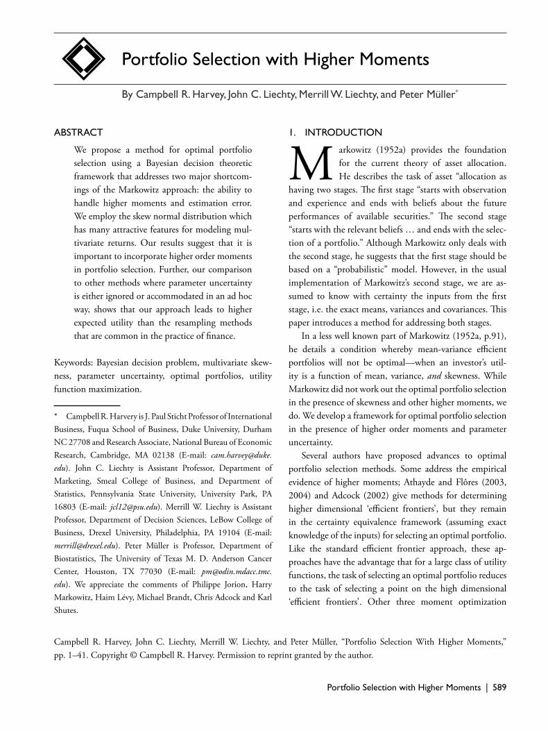
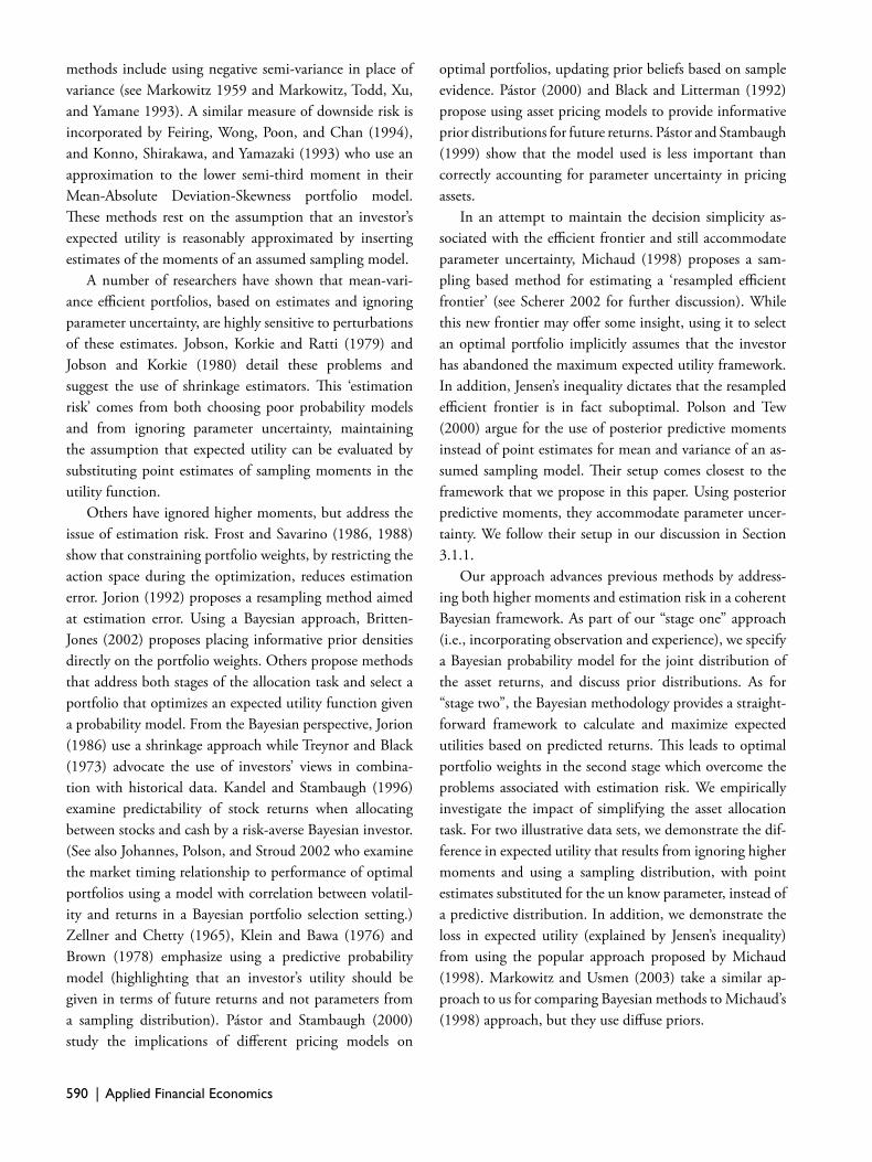
Our investigation of multiple assets builds on these empirical fi ndings and indicates that the existence of ‘co-skewness’, which can be interpreted as correlated extremes, is often hidden when assets are considered one at a time. To illustrate, Figure 1 contains the kernel density estimate

and normal distribution for the marginal daily returns of two stocks (Cisco Systems and General Electric from April 1996 to March 2002) and Figure 2 contains a bivariate normal approximation of their joint returns. While the marginal summaries in Figure 1 suggest almost no devia-tion from the normality assumption, the joint summary appears to exhibit a degree of coskewness, suggesting that skewness may have a larger impact on the distribution of a portfolio than previously anticipated.

2.1 Economic Importance

Markowitz’s intuition for maximizing the mean while minimizing the variance of a portfolio comes from the idea that the investor prefers higher expected returns and lower risk. Extending this concept further, most agree that ceteris paribus investors prefer a high probability of an extreme event in the positive direction over a high probability of an extreme event in the negative direction. From a theoretical perspective, Markowitz (1952b) and Arrow (1971) argue that desirable utility functions should exhibit decreasing absolute risk aversion, implying that investors should have preference for positively skewed asset returns. (Also see the discussion in Roy 1952.) Experimental evidence of prefer-ence for positively skewed returns has been established by Sortino and Price (1994) and Sortino and Forsey (1996) for example. Lévy and Sarnat (1984) fi nd a strong preference for positive skewness in the study of mutual funds. Harvey and Siddique (2000a,b) introduce an asset pricing model that incorporates conditional skewness, and show that an investor may be willing to accept a negative expected return in the presence of high positive skewness.

An aversion towards negatively skewed returns sum-marizes the basic intuition that many investors are will-ing to trade some of their average return for a decreased chance that they will experience a large reduction in their wealth, which could signifi cantly reduce their level of consumption. Some researchers have attempted to address aversion to negative returns in the asset allocation problem by abandoning variance as a measure of risk and defi ning a ‘downside’ risk that is based only on negative returns. Th ese attempts to separate “good” and “bad” variance can be formalized in a consistent framework by using utility functions and probability models that account for higher moments.

While skewness will be important to a large class of investors and is evident in the historical returns of the


underlying assets and portfolios, the question remains; how infl uential is skewness in terms of fi nding optimal portfolio weights? Cremers, Kritzman, and Page (2004) argue that only under certain utility is it worthwhile to consider skew-ness in portfolio selection. However, it is our experience that any utility function approximated by a third order Taylor’s expansion can lead to more informatively selected portfolio weights if skewness is not ignored.

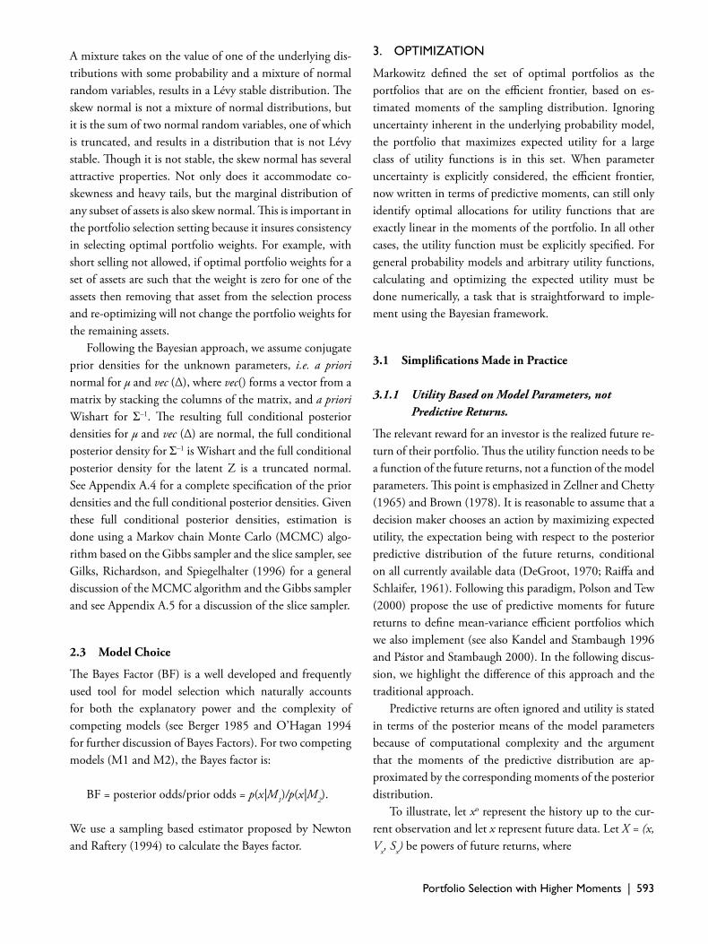
To illustrate, consider the impact of skewness on the empirical distribution of a collection of two-stock portfo-lios. For each portfolio, the mean is identical to the linear combination of the stock means and the variance is less than the combination of the stock variances, see Figure 3 for an illustration using three, two-stock portfolios. Unlike the variance, there is no guarantee that the portfolio skewness will be larger or smaller than the linear combination of the stock skewness, and in practice we observe a wide variety of behavior. Th is suggests that the mean-variance optimal criteria will lead to sub-optimal portfolios in the presence of skewness. To accommodate higher-order moments in the asset allocation task, we must introduce an appropriate probability model. After providing an overview of possible approaches, we formally state a model and discuss model choice tools.

2.2 Probability Models for Higher Moments

Th ough it is a simplifi cation of reality, a model can be informative about complicated systems. While the multi-variate normal distribution has several attractive properties for modeling a portfolio, there is considerable evidence that portfolio returns are non-normal. Th ere are a number of alternative models that include higher moments. Th e multivariate Student t-distribution is good for fat tailed data, but does not allow for asymmetry. Th e non-central multivariate t-distribution also has fat tails and, in addi-tion, is skewed. However, the skewness is linked directly to the location parameter and is, therefore, somewhat infl ex-ible. Th e log-normal distribution has been used to model asset returns, but its skewness is a function of the mean and variance, not a separate skewness parameter.

Azzalini and Dalla Valle (1996) propose a multivariate skew normal distribution that is based on the product of a multivariate normal probability density function (pdf ) and univariate normal cumulative distribution function (cdf ). Th is is generalized into a class of multivariate skew ellipti-cal distributions by Branco and Dey (2001), and improved

upon by Sahu, Branco and Dey (2003) by using a multi-variate cdf instead of univariate cdf, adding more fl exibility, which often results in better fi tting models. Because of the importance of coskewness in asset returns, we start with the multivariate skew normal probability model presented in Sahu et al. (2003) and off er a generalization of their model.

Th e multivariate skew normal can be viewed as a mix-ture of an unrestricted multivariate normal density and a truncated, latent multivariate normal density, or

X = μ +ΔZ + є, (1)

where μ and Δ are an unknown parameter vector and matrix respectively, ϵ is a normally distributed error vec-tor with a zero mean and covariance Σ, and Z is a vector of latent random variables. Z comes from a multivariate normal with mean 0 and an identity covariance matrix and is restricted to be non-negative, or

(2)where I{•} is the indicator function and Zj is the jth element of Z. In Sahu et al. (2003), Δ is restricted to being a diagonal matrix, which accommodates skewness, but does not allow for coskewness. We generalize the Sahu et al. (2003) model to allow Δ to be an unrestricted random matrix resulting in a modifi ed density and moment generating function, see Appendix A.1 for details.

As with other versions of the skew normal model, this model has the desirable property that marginal distribu-tions of subsets of skew normal variables are skew normal (see Sahu et al. 2003 for a proof ). Unlike the multivariate normal density, linear combinations of variables from a multivariate skewed normal density are not skew normal. Th is does not, however, restrict us from calculating mo-ments of linear combinations with respect to the model parameters, see Appendix A.2 for the formula for the fi rst three moments.

Even though they can be written as the sum of a normal and a truncated normal random variable, neither the skew normal of Azzalini and Dalla Valle (1996) nor Sahu et al. (2003) are Lévy stable distributions. Th e skew normal can be generalized as a stable distribution (see Appendix A.3).

While the skew normal is similar in concept to a mixture of normal random variables, it is fundamentally diff erent.


A mixture takes on the value of one of the underlying dis-tributions with some probability and a mixture of normal random variables, results in a Lévy stable distribution. Th e skew normal is not a mixture of normal distributions, but it is the sum of two normal random variables, one of which is truncated, and results in a distribution that is not Lévy stable. Th ough it is not stable, the skew normal has several attractive properties. Not only does it accommodate co-skewness and heavy tails, but the marginal distribution of any subset of assets is also skew normal. Th is is important in the portfolio selection setting because it insures consistency in selecting optimal portfolio weights. For example, with short selling not allowed, if optimal portfolio weights for a set of assets are such that the weight is zero for one of the assets then removing that asset from the selection process and re-optimizing will not change the portfolio weights for the remaining assets.

Following the Bayesian approach, we assume conjugate prior densities for the unknown parameters, i.e. a priori normal for μ and vec (Δ), where vec() forms a vector from a matrix by stacking the columns of the matrix, and a priori Wishart for Σ–1. Th e resulting full conditional posterior densities for μ and vec (Δ) are normal, the full conditional posterior density for Σ–1 is Wishart and the full conditional posterior density for the latent Z is a truncated normal. See Appendix A.4 for a complete specifi cation of the prior densities and the full conditional posterior densities. Given these full conditional posterior densities, estimation is done using a Markov chain Monte Carlo (MCMC) algo-rithm based on the Gibbs sampler and the slice sampler, see Gilks, Richardson, and Spiegelhalter (1996) for a general discussion of the MCMC algorithm and the Gibbs sampler and see Appendix A.5 for a discussion of the slice sampler.

2.3 Model Choice

Th e Bayes Factor (BF) is a well developed and frequently used tool for model selection which naturally accounts for both the explanatory power and the complexity of competing models (see Berger 1985 and O’Hagan 1994 for further discussion of Bayes Factors). For two competing models (M1 and M2), the Bayes factor is:

BF = posterior odds/prior odds = p(x|M1)/p(x|M2).

We use a sampling based estimator proposed by Newton and Raftery (1994) to calculate the Bayes factor.

3. OPTIMIZATION

Markowitz defi ned the set of optimal portfolios as the portfolios that are on the effi cient frontier, based on es-timated moments of the sampling distribution. Ignoring uncertainty inherent in the underlying probability model, the portfolio that maximizes expected utility for a large class of utility functions is in this set. When parameter uncertainty is explicitly considered, the effi cient frontier, now written in terms of predictive moments, can still only identify optimal allocations for utility functions that are exactly linear in the moments of the portfolio. In all other cases, the utility function must be explicitly specifi ed. For general probability models and arbitrary utility functions, calculating and optimizing the expected utility must be done numerically, a task that is straightforward to imple-ment using the Bayesian framework.

3.1 Simplifi cations Made in Practice

3.1.1 Utility Based on Model Parameters, not Predictive Returns.

Th e relevant reward for an investor is the realized future re-turn of their portfolio. Th us the utility function needs to be a function of the future returns, not a function of the model parameters. Th is point is emphasized in Zellner and Chetty (1965) and Brown (1978). It is reasonable to assume that a decision maker chooses an action by maximizing expected utility, the expectation being with respect to the posterior predictive distribution of the future returns, conditional on all currently available data (DeGroot, 1970; Raiff a and Schlaifer, 1961). Following this paradigm, Polson and Tew (2000) propose the use of predictive moments for future returns to defi ne mean-variance effi cient portfolios which we also implement (see also Kandel and Stambaugh 1996 and Pástor and Stambaugh 2000). In the following discus-sion, we highlight the diff erence of this approach and the traditional approach.

Predictive returns are often ignored and utility is stated in terms of the posterior means of the model parameters because of computational complexity and the argument that the moments of the predictive distribution are ap-proximated by the corresponding moments of the posterior distribution.

To illustrate, let xo represent the history up to the cur-rent observation and let x represent future data. Let X = (x, Vx, Sx) be powers of future returns, where


is the predictive mean given xo, Vx = (x – mp)(x –mp)׳, and Sx = Vx (x –mp)׳. Assuming that utility is a third-order polynomial of future returns, predictive utility is given by

(3)where λ and γ determine the impact of predictive variance and skewness. Expected utility, becomes

where θp = (mp, Vp, Sp) are the predictive moments of x. We refer to utility function (3) as a linear utility function. Utility is linear in the sense that upred is linear in the predic-tive summaries X, and thus EUpred is linear in the predictive moments θp.

Often a function involving sampling moments corre-sponding to the predictive moments in (4) is used instead of actual future returns to defi ne utility. Assuming an i.i.d. sampling xt ~ pθ(xt) for returns at time t, let θ = (m, V, S) denote the moments of pθ and defi ne a utility function:

(5)See Appendix A.1 for the formulas under the skew normal model. Th e expected utility, becomes

(6)where m ,V and S are the posterior means of θ. Note that the expectation in (6) “plugs in” the expectation of the parameters, ignoring the contribution of parameter un-certainty to the expected utility function. (Kan and Zhou (2004) provide a thorough discussion of the diff erence of plug-in and Bayes estimator of the optimal decision under the parameter based utility (5). Th eir discussion highlights the diff erence between a proper Bayes rule, defi ned as the decision that maximizes expected utility, versus a rule that plugs in the Bayes estimate for the weights or the parameters in the sampling distribution.) Th e nature of this approxi-mation is highlighted by considering the relationship with

the predictive moments in (4). In fact, it is straightforward to show that the predictive mean equals the posterior mean and that the predictive variance and skewness equal the posterior means of V and S plus additional terms, or

Polson and Tew (2000, proposition 1) highlight the implication of the diff erence between Vp and V for mean-variance effi cient portfolios. Substituting this into (4) gives an alternative form that is composed of EUparam(ω) plus other terms.

For linear utility functions, stating utility in terms of the probability model parameters implicitly assumes that the predictive variance and skewness are approximately equal to the posterior expectation of m, V , and S, an assump-tion which often fails in practice. Formally, using (m, V , S) in place of the predictive moments ignores the second and third line in the expression above. Our approach uses the predictive moments, capturing that extra information when maximizing the expected utility.

3.1.2 Maximize Something Other Th an Expected Utility.

Given that utility functions can be diffi cult to integrate, various approximations are often used. Th e simplest ap-proximation is to use a fi rst-order Taylor’s approximation (see Novshek 1993) about the expected predictive sum-maries, or assume

For linear utility functions this approximation is exact, as in (3) and (4). Th e Taylor’ approximation removes any


parameter uncertainty and leads directly to the certainty equivalence optimization framework, substituting predic-tive moments. It is easy to see that combining the Taylor’s approximation and the much stronger assumption that the posterior moments approximately equal predictive moments leads to a frequently used ‘two-time removed’ approximation of the expected utility of future returns, or

In an attempt to maintain the fl exibility of the effi cient frontier optimization framework but still accommodate parameter uncertainty, Michaud (1998) proposes an op-timization approach that switches the order of integration (averaging) and optimization. Th e maximum expected utility framework optimizes the expected utility of future returns; the certainty equivalence framework optimizes the utility of expected future returns, (i.e., substituting poste-rior predictive moments in the utility function). Michaud (1998) proposes creating a ‘resampled frontier’ by repeat-edly maximizing the utility for a draw from a probability distribution and then averaging the optimal weights that result from each optimization. While the approach could be viewed in terms of predictive returns, the sampling guidelines are arbitrary and could signifi cantly impact the results. Given, that the main interest is to account for parameter uncertainty, we consider a modifi ed algorithm where parameter draws from a posterior density are used in place of the predictive moment summaries. To be explicit, assuming a utility of parameters, the essential steps of the algorithm are as follows. For a family of utility functions (uparam,1, …, uparam,K), perform the following steps.

1. For each utility function (e.g. uparam,k), generate n draws from a posterior density

2. For each fi nd weight that maximizes

3. For each utility function, let defi ne the optimal portfolio.

By Jensen’s inequality if ,then for a large class of utility functions

(7)

Further if maximizes , then

for all . From (7), clearly

or results in a sub-optimal portfolio in terms of ex-pected utility maximization. Stated in practical terms, on average, Michaud’s approach ‘leaves money on the table’.

3.1.3 Ignore Skewness.

Although evidence of skewness and other higher moments in fi nancial data are abundant, it is common for skewness to be ignored entirely in practice. Typically skewness is ignored both in the sampling models and in the assumed utility functions. In order to illustrate the impact of ignor-ing skewness, Figure 4 shows the empirical summary of the distribution of possible portfolios for four equity securities (Cisco Systems, General Electric, Sun Microsystems, and Lucent Technologies). Th e mean-variance summary imme-diately leads to Markowitz’s initial insight, but the relation-ship between mean, variance and skewness demonstrates that Markowitz’s two-moment approach off ers no guidance for making eff ective trade off s between mean, variance and skewness. Using the certainty equivalence framework and a linear utility of the fi rst three empirical moments, or

where me, Ve, Se are the empirical mean, variance and skew-ness, Figure 5 contrasts the optimal portfolios that result from assuming an investor only has an aversion to variance (λ = 0.5, γ = 0) and has both an aversion to variance and a preference for positive skewness (λ = 0.5, γ = 0.5).

When skewness is considered, the optimal portfolio is pushed further up the effi cient frontier signifying that for the same level of risk aversion, an investor can get a higher return if they include skewness in the decision process. In this case, the positive skewness of the portfolio eff ectively reduces the portfolio risk.

3.2 Bayesian Optimization Methods

Bayesian methods off er a natural framework for both, the evaluation of expectations and the optimization of expect-ed utilities for an arbitrary utility function, with respect to an arbitrarily complicated probability model. Given


an appropriate Markov chain Monte Carlo (MCMC) estimation routine, it is straightforward and computation-ally trivial to generate draws from the posterior predictive density, or to draw by computer simulation

and then evaluate the predictive summaries Xi. Given a set of n draws, the expected utility for an arbitrary utility function can be estimated as an ergodic average, or

Th e approximate expected utility can then be optimized numerically using a number of diff erent approaches. One attractive algorithm is the Metropolis-Hastings (MH) algorithm. MH simulation is widely used for posterior simulation. But the same algorithm can be exploited for expected utility optimization. When used for formal op-timization, it is known as simulated annealing. Stopping short of simulated annealing, we use the MH algorithm to explore the expected utility function, f(ω) = E[U(ω)], as a function of the weights. Asymptotic properties of the MH chain lead to portfolio weights ω being generated with frequencies proportional to EU(ω). Th at is, promis-ing portfolio weights with high expected utility are visited more often, as desired. See, for example, Gilks et al. (1996) and Meyn and Tweedie (1993) for a discussion of the MH algorithm. Intuitively, this Markov chain can be viewed as a type of ‘random walk’ with a drift in the direction of larger values of the target function. When the MH algorithm is used as a tool for performing statistical inference, the target density is typically a posterior probability density; however, this need not be the case. As long as the target function is non-negative and integrable, the MH can be used to numerically explore any target function. Not only has the MH been shown to be very eff ective for searching high dimensional spaces, its irreducible property ensures, that if a global maximum exists the MH algorithm will eventually escape from any local maximum and visit the global maximum.

In order to use the MH function, we need to ensure that our expected utility is nonnegative and integrable. For the linear utility functions, integrability over the space of possible portfolios, where the portfolios are restricted to the unit simplex (i.e. we do not allow short selling), is easily established. We modify the utility function so that

it is a non-negative function by subtracting the minimum expected utility, or the target function becomes

4. OPTIMAL PORTFOLIOS IN PRACTICE

In theory, simplifi cations of the complete asset allocation task will result in a sub-optimal portfolio selection. In order to assess the impact that results from some of these simplifi cations in practice, we consider three diff erent optimization approaches for two data sets using a family of linear utility functions. In particular, we consider the utility functions given in (3) and (5), which have expected utilities given in terms of the predictive posterior and pos-terior moments respectively, see (4) and (6). We consider a number of potential probability models and select the best model. Using results from both the multivariate normal model and the best higher moment model, we numerically determine the optimal portfolio based on the predictive returns, the parameter values and using Michaud’s (1998) non-utility maximization approach. We contrast the per-formance of each optimal portfolio in terms of expected predictive utility using the best model.

4.1 Data Description

We consider two sets of returns. Th e fi rst set comes from four equity securities. Th e second set comes from a broad-based portfolio of domestic and international equities and fi xed income.

First we consider daily returns from April 1996 to March 2002 on four equity securities consisting of General Electric, Lucent Technologies, Cisco Systems, and Sun Microsystems. Th ese stocks are from the technology sec-tor, and are chosen to illustrate portfolio selection among closely related assets.

We also try to select securities that match the asset allo-cation choices facing individuals. To do so we consider the weekly returns from January 1989 to June 2002 on four equity portfolios: Russell 1000 (large capitalization stocks), Russell 2000 (smaller capitalization stocks), Morgan Stanley Capital International (MSCI) EAFE (non-U.S. developed markets), and MSCI EMF (emerging market equities that are available to international investors). We consider three fi xed income portfolios: government bonds, corporate bonds, and mortgage backed bonds. Each of


Table 1. Evaluating the Distributional Representation of Four Equity Securities and global asset allocation benchmarks

Model choice results for analysis of the daily stock returns of General Electric, Lucent Technologies, Cisco Systems, and Sun Microsystems from April 1996 to March 2002. And also for weekly benchmark indices from January 1989 to June 2002 (Lehman Brothers government bonds, LB corporate bonds, and LB mortgage bonds, MSCI EAFE (non-U.S. developed market equity), MSCI EMF (emerging market free investments), Russell 1000 (large cap), and Russell 2000 (small cap)). Th e four models that are used are the multivariate normal (MV-Normal), the multivariate skew normal of Azzalini and Dalla Valle (1996) with a diagonal Δ matrix (MVS-Normal D-Δ), and the multivariate skew normal of Sahu et al. (2003) with both a diagonal and full Δ matrix (MVS-Normal F-Δ). Maximum log likelihood values are used to compute Bayes factors between the multivariate normal model and all of the other models and is reported on the log scale. Th e model with the highest Bayes factor best fi ts the data. Sahu et al. (2003) diagonal Δ model fi ts best overall.

a. Four equity securities

b. Global asset allocation benchmarks


these fi xed income return series are from Lehman Brothers and form the three major subcomponents of the popular Lehman aggregate index.

4.2 Model Choice and Select Summary Statistics

To determine which skew normal model best fi t the respective data sets, we compute Bayes factors for the multivariate normal model, the skew normal model pro-posed by Azzalini and Dalla Valle (1996) with a diagonal Δ matrix, and the skew normal model proposed by Sahu et al. (2003) with both a diagonal and our modifi ed full Δ matrix. Th e results for the technology stocks shows that the skew normal models with a diagonal Δ outperform the other models, with the Sahu et al. (2003) model fi tting best. Th e skew normal model with the full Δ, however, per-forms better than the others in the case of the benchmark indices (see Table 1). Th e model with the full Δ accom-modates coskewness, which could be viewed as correlated extremes, better than the model with the diagonal Δ. Th is suggests that portfolios of highly related stocks may have less coskewness than portfolios of highly diversifi ed global summaries.

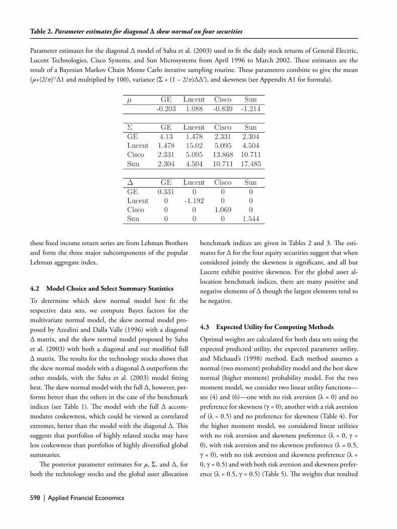
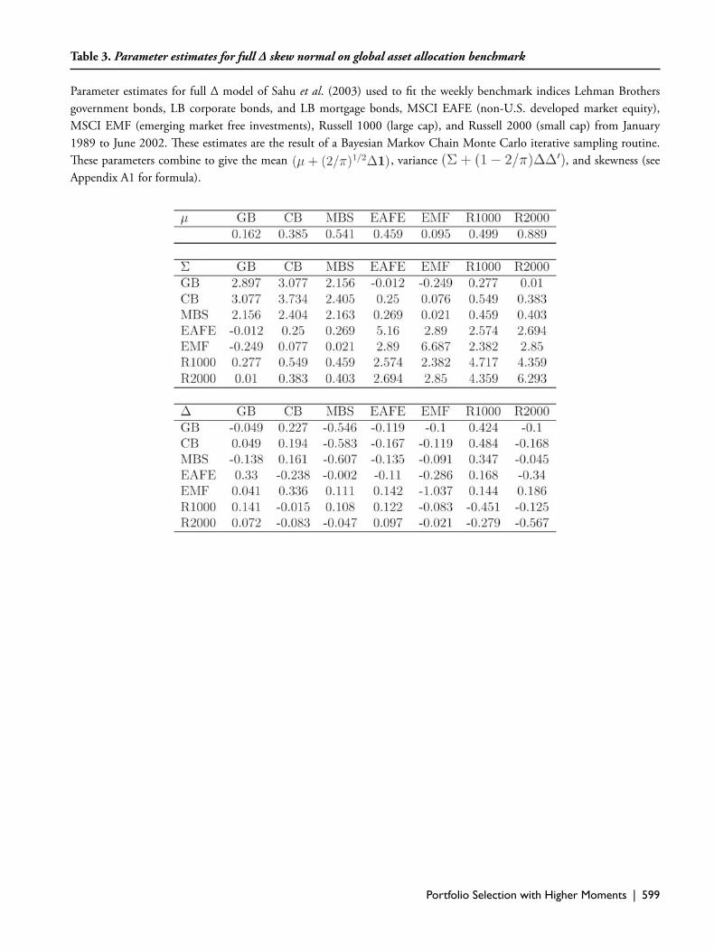
Th e posterior parameter estimates for μ, Σ, and Δ, for both the technology stocks and the global asset allocation

benchmark indices are given in Tables 2 and 3. Th e esti-mates for Δ for the four equity securities suggest that when considered jointly the skewness is signifi cant, and all but Lucent exhibit positive skewness. For the global asset al-location benchmark indices, there are many positive and negative elements of Δ though the largest elements tend to be negative.

4.3 Expected Utility for Competing Methods

Optimal weights are calculated for both data sets using the expected predicted utility, the expected parameter utility, and Michaud’s (1998) method. Each method assumes a normal (two moment) probability model and the best skew normal (higher moment) probability model. For the two moment model, we consider two linear utility functions— see (4) and (6)—one with no risk aversion (λ = 0) and no preference for skewness (γ = 0); another with a risk aversion of (λ = 0.5) and no preference for skewness (Table 4). For the higher moment model, we considered linear utilities with no risk aversion and skewness preference (λ = 0, γ = 0), with risk aversion and no skewness preference (λ = 0.5, γ = 0), with no risk aversion and skewness preference (λ = 0, γ = 0.5) and with both risk aversion and skewness prefer-ence (λ = 0.5, γ = 0.5) (Table 5). Th e weights that resulted

Table 2. Parameter estimates for diagonal Δ skew normal on four securities

Parameter estimates for the diagonal Δ model of Sahu et al. (2003) used to fi t the daily stock returns of General Electric, Lucent Technologies, Cisco Systems, and Sun Microsystems from April 1996 to March 2002. Th ese estimates are the result of a Bayesian Markov Chain Monte Carlo iterative sampling routine. Th ese parameters combine to give the mean (μ+(2/π)½ Δ1 and multiplied by 100), variance (Σ + (1 – 2/π)ΔΔ’), and skewness (see Appendix A1 for formula).


Table 3. Parameter estimates for full Δ skew normal on global asset allocation benchmark

Parameter estimates for full Δ model of Sahu et al. (2003) used to fi t the weekly benchmark indices Lehman Brothers government bonds, LB corporate bonds, and LB mortgage bonds, MSCI EAFE (non-U.S. developed market equity), MSCI EMF (emerging market free investments), Russell 1000 (large cap), and Russell 2000 (small cap) from January 1989 to June 2002. Th ese estimates are the result of a Bayesian Markov Chain Monte Carlo iterative sampling routine. Th ese parameters combine to give the mean , variance , and skewness (see Appendix A1 for formula).


Table 4. Two and three moment optimization for four equity securities

Th is table contains predictive utilities for the weights that maximize utility as a linear function of the two and three moments of the multivariate normal model by three diff erent methods for daily stock returns of General Electric, Lucent Technologies, Cisco Systems, and Sun Microsystems from April 1996 to March 2002. Th e fi rst method is based on predic-tive or future values of the portfolio (results in ωi,pred where the i represents the number of moments in the model), the second is based on the posterior parameter estimates (ωi,param), and the third is the method proposed by Michaud (ωi,Michaud). Th e weights that are found by each method are ranked by the three moment predictive utility they produce (i.e E[u3,pred(ω)] = ω′mp – λω′Vpω + γ ω′Spω ω,where the 3 signifi es that the utility function is linear in the fi rst three moments of the skew normal model, and mp, Vp, and Sp are the predictive mean, variance and skewness) for varying values of λ and γ. Th e highest utility obtained signifi es the method that is best for portfolio selection according to the investor’s preferences. For each combination of λ and γ, ωi,pred gives the highest expected utility.

a. Two moments

b. Th ree moments


Table 5. Two and three moment optimization for global asset allocation benchmark indices

Predictive utilities for the weights that maximize utility as a linear function of the two and three moments of the multi-variate normal model by three diff erent methods for weekly benchmark indices Lehman Brothers government bonds, LB corporate bonds, and LB mortgage bonds, MSCI EAFE (non–U.S. developed market equity), MSCI EMF (emerging market free investments), Russell 1000 (large cap), and Russell 2000 (small cap) from January 1989 to June 2002. Th e fi rst method is based on predictive or future values of the portfolio (results in ωi,pred where the i represents the number of moments in the model), the second is based on the posterior parameter estimates (ωi,param), and the third is the method proposed by Michaud (ωi,Michaud). Th e weights that are found by each method are ranked by the three moment predictive utility they produce (i.e E[u3,pred(ω)] = ω′mp - λ ω′Vp ω + γ ω′Sp ω ω, where the 3 signifi es that the utility function is linear in the fi rst three moments of the skew normal, and mp, Vp, and Sp are the predictive mean, variance and skewness) for varying values of λ and γ. Th e highest utility obtained signifi es the method that is best for portfolio selection according to the investor’s preferences. For each combination of λ and γ, ωi,pred gives the highest expected utility.

a. Two moments

b. Th ree moments


from each optimization were then used to calculate the expected predictive utility.

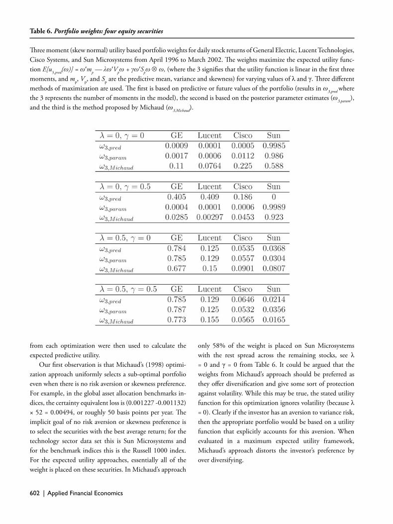
Our fi rst observation is that Michaud’s (1998) optimi-zation approach uniformly selects a sub-optimal portfolio even when there is no risk aversion or skewness preference. For example, in the global asset allocation benchmarks in-dices, the certainty equivalent loss is (0.001227 -0.001132) × 52 = 0.00494, or roughly 50 basis points per year. Th e implicit goal of no risk aversion or skewness preference is to select the securities with the best average return; for the technology sector data set this is Sun Microsystems and for the benchmark indices this is the Russell 1000 index. For the expected utility approaches, essentially all of the weight is placed on these securities. In Michaud’s approach

only 58% of the weight is placed on Sun Microsystems with the rest spread across the remaining stocks, see λ = 0 and γ = 0 from Table 6. It could be argued that the weights from Michaud’s approach should be preferred as they off er diversifi cation and give some sort of protection against volatility. While this may be true, the stated utility function for this optimization ignores volatility (because λ = 0). Clearly if the investor has an aversion to variance risk, then the appropriate portfolio would be based on a utility function that explicitly accounts for this aversion. When evaluated in a maximum expected utility framework, Michaud’s approach distorts the investor’s preference by over diversifying.

Table 6. Portfolio weights: four equity securities

Th ree moment (skew normal) utility based portfolio weights for daily stock returns of General Electric, Lucent Technologies, Cisco Systems, and Sun Microsystems from April 1996 to March 2002. Th e weights maximize the expected utility func-tion E[u3,pred(ω)] = ω′mp — λω′Vpω + γω′Spω ω, (where the 3 signifi es that the utility function is linear in the fi rst three moments, and mp, Vp, and Sp are the predictive mean, variance and skewness) for varying values of λ and γ. Th ree diff erent methods of maximization are used. Th e fi rst is based on predictive or future values of the portfolio (results in ω3,pred where the 3 represents the number of moments in the model), the second is based on the posterior parameter estimates (ω3,param), and the third is the method proposed by Michaud (ω3,Michaud).


Not surprisingly, when there is only preference for skewness, the predictive optimization approach outper-forms the parameter approach, e.g. λ = 0, γ = 0.5 in Table 4. Th is diff erence illustrates the fact that the predictive vari-ance and skewness are only approximated by the estimates of the variance and skewness based on posterior parameter values, see Section 3.1. In the case of the technology stocks, with λ = 0 and γ = 0.5, the parameter optimization ap-proach places almost all of the portfolio weight on Sun Microsystems, but in light of predictive skewness the predictive approach distributes almost all of the weight on the three other stocks, see Table 6.

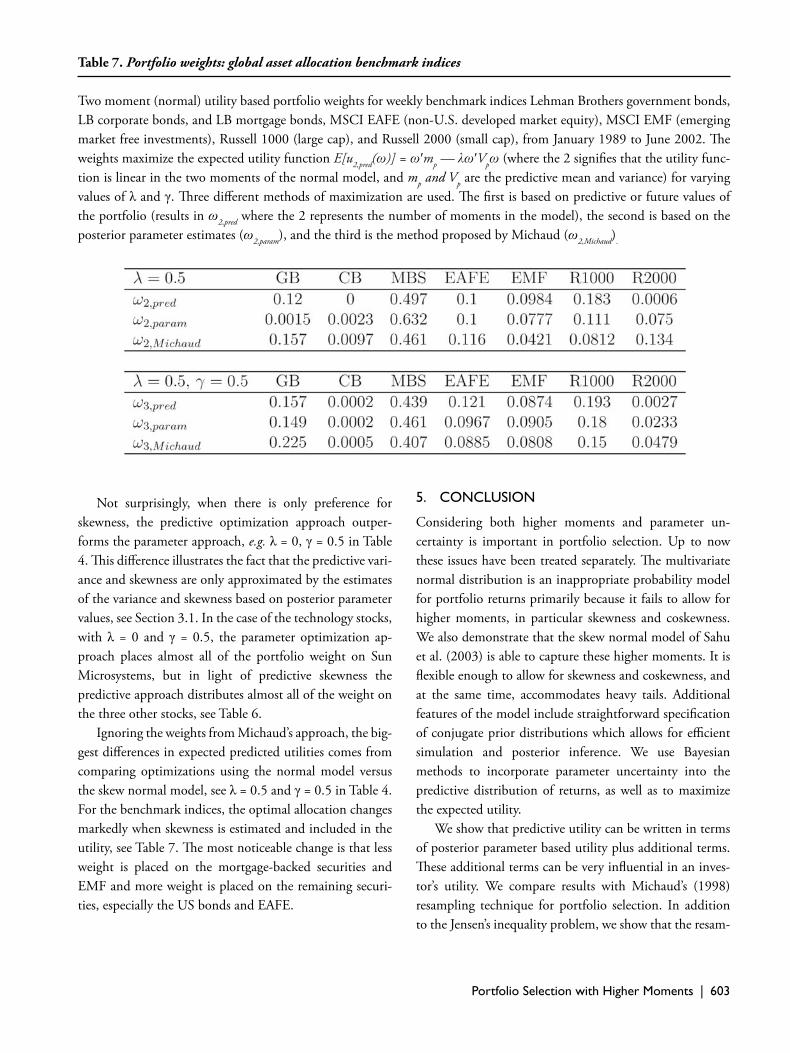
Ignoring the weights from Michaud’s approach, the big-gest diff erences in expected predicted utilities comes from comparing optimizations using the normal model versus the skew normal model, see λ = 0.5 and γ = 0.5 in Table 4. For the benchmark indices, the optimal allocation changes markedly when skewness is estimated and included in the utility, see Table 7. Th e most noticeable change is that less weight is placed on the mortgage-backed securities and EMF and more weight is placed on the remaining securi-ties, especially the US bonds and EAFE.

5. CONCLUSION

Considering both higher moments and parameter un-certainty is important in portfolio selection. Up to now these issues have been treated separately. Th e multivariate normal distribution is an inappropriate probability model for portfolio returns primarily because it fails to allow for higher moments, in particular skewness and coskewness. We also demonstrate that the skew normal model of Sahu et al. (2003) is able to capture these higher moments. It is fl exible enough to allow for skewness and coskewness, and at the same time, accommodates heavy tails. Additional features of the model include straightforward specifi cation of conjugate prior distributions which allows for effi cient simulation and posterior inference. We use Bayesian methods to incorporate parameter uncertainty into the predictive distribution of returns, as well as to maximize the expected utility.

We show that predictive utility can be written in terms of posterior parameter based utility plus additional terms. Th ese additional terms can be very infl uential in an inves-tor’s utility. We compare results with Michaud’s (1998) resampling technique for portfolio selection. In addition to the Jensen’s inequality problem, we show that the resam-

Table 7. Portfolio weights: global asset allocation benchmark indices

Two moment (normal) utility based portfolio weights for weekly benchmark indices Lehman Brothers government bonds, LB corporate bonds, and LB mortgage bonds, MSCI EAFE (non-U.S. developed market equity), MSCI EMF (emerging market free investments), Russell 1000 (large cap), and Russell 2000 (small cap), from January 1989 to June 2002. Th e weights maximize the expected utility function E[u2,pred(ω)] = ω′mp — λω′Vpω (where the 2 signifi es that the utility func-tion is linear in the two moments of the normal model, and mp and Vp are the predictive mean and variance) for varying values of λ and γ. Th ree diff erent methods of maximization are used. Th e fi rst is based on predictive or future values of the portfolio (results in ω2,pred where the 2 represents the number of moments in the model), the second is based on the posterior parameter estimates (ω2,param), and the third is the method proposed by Michaud (ω2,Michaud).


pling approach is outside the effi cient utility maximization framework.

While we believe that we have made progress on two important issues in portfolio selection, there are at least three limitations to our approach. First, our information is restricted to past returns. Th at is, investors make decisions based on past returns and do not use other conditioning information such as economic variables that tell us about the state of the economy. Second, our exercise is an ‘in-sample’ portfolio selection. We have not applied our method to out-of sample portfolio allocation. Finally, the portfolio choice problem we examine is a static one. Th ere is a growing literature that considers the more challenging dynamic asset allocation problem that allows for portfolio weights to change with investment horizon, labor income and other economic variables.

We believe that it is possible to make progress in future research on the fi rst two limitations. In addition, we are interested in using revealed market preferences to deter-mine whether ‘the market’ empirically exhibits preference for skewness. As a fi rst step, we plan to use the observed market weights for a benchmark equity index and use the predictive utility function (3) to determine the implied market λ and γ. Finally, we intend to consider modifi ca-tions to (3) that allow for asymmetric preferences over positive and negative skewness.

REFERENCES

Adcock, C. J. (2002), “Asset Pricing and Portfolio Selec-tion Based on the Multivariate Skew-Student Distri-bution,” paper presented at the Non-linear Asset Pricing Workshop, April, Paris.

Arrow, K. J. (1971), “Essays in the Th eory of Risk-Bear-ing,” Chicago: Markham Publishing Co.

Athayde, G. M. de, and Flores, R. G. Jr. (2003), “Advances in Portfolio Construction and Implementation”, Satch-ell and Scowcroft, eds.

—— (2004), “Finding a maximum skewness portfolio–a general solution to three moments portfolio choice,” Journal of Economic Dynamics and Control, vol. 28, is-sue 7, 1335–1352.

Azzalini, A., and Dalla Valle, A. (1996), “Th e Multivariate Skew-Normal Distribution,” Biometrika, 83, 715–726.

Berger, J. (1985), “Statistical Decision Th eory and Bayes-ian Analysis,” New York, NY: Springer Veralg .

Black, F., and Litterman, R. (1992), “Global portfolio optimization,” Financial Analysts Journal, September-October 1992.

Branco, M. D., and Dey, D. K. (2001), “A General Class of Multivariate Skew-Elliptical Distributions,” Journal of Multivariate Analysis, 79, 99–113.

Britten-Jones, M. (2002), “Portfolio optimization and Bayesian regression,” Unpublished working paper, Lon-don Business School.

Brown, S. J. (1978), “Th e portfolio choice problem: Com-parison of certainty equivalent and optimal Bayes port-folios,” Communications in Statistics: Simulation and Computation B7, 321–334.

Cascon, A., Keating, C., and Shadwick, W. F. (2003), “Th e Omega Function,” working paper.

Cremers, J-H., Kritzman, M., and Page, S. (2004), “Port-folio Formation with Higher Moments and Plausible Utility,” Working paper.

Damien, P. S., Wakefi eld, J., and Walker, G. (1999), “Gibbs Sampling For Bayesian Nonconjugate and Hi-erarchical Models Using Auxilliary Variables,” Journal of Royal Statistical Society, Ser. B, 61, Part 2, 331-344.

DeGroot, M. H. (1970), “Optimal Statistical Decisions,” New York: McGraw-Hill.

Feiring, B. R., Wong, W., Poon, M., and Chan, Y. C. (1994), “Portfolio Selection in Downside Risk Optimi-zation Approach: Application to the Hong Kong Stock Market,” International Journal of Systems Science, 25, 1921–1929.

Frost, P. A., and Savarino, J. E. (1986), “An Empirical Bayes Approach to Effi cient Portfolio Selection,” Jour-nal of Financial and Quantitative Analysis, 21, No. 3, 293–305.

—— (1988), “For better performance; Constrain portfolio weights,” Journal of Portfolio Management, 14, 29–34

Gilks, W. R., Richardson, S., and Spiegelhalter, D. J. (1996), “Markov Chain Monte Carlo in Practice,” Chapman and Hall, London.

Harvey, C. R., and Siddique, A. (2000a), “Conditional Skewness in Asset Pricing Tests,” Journal of Finance, 55, 1263–1295

—— (2000b), “Time-Varying Conditional Skewness and the Market Risk Premium,” Research in Banking and Fi-nance, 1, 27–60.

Jobson, J. D., Korkie, B., and Ratti, V. (1979), “Improved estimation for Markowitz portfolios using James-Stein type estimators,” Proceedings of the American Statistical


Association, Business and Economic Statistics Section, 279–284.

Jobson, J. D., and Korkie, B. (1980), “Estimation of Mar-kowitz effi cient portfolios,” Journal of the American Sta-tistical Association 75, 544–554.

Johannes, M., Polson, N., and Stroud, J. (2002), “Sequen-tial Optimal Portfolio Performance: Market and Vola-tility Timing,” Unpublished working paper.

Jorion, P. (1992), “Portfolio Optimization in Practice,” Fi-nancial Analysts Journal, January/February 68–74.

—— (1986), “Bayes-Stein Estimation of Portfolio Analy-sis,” Journal of Financial and Quantitative Analysis, 21, 279–292.

Kan, R., and Zhou, G. (2004), “Optimal Estimation for Economic Gains: Portfolio Choice with Parameter Un-certainty,” Working paper, Washington University, St. Louis.

Kandel, S., and Stambaugh, R. F. (1996), “On the predict-ability of stock returns: An asset allocation perspective,” Journal of Finance, 51, 2, 385–424.

Klein, R. W., and Bawa, V. (1976), “Th e eff ect of estima-tion risk on optimal portfolio choice,” Journal of Finan-cial Economics, 3, 215–231.

Kon, S. (1984), “Models of Stock Returns - a Compari-son,” Journal of Finance, 39, 147–165.

Konno, H., Shirakawa, H., and Yamazaki, H. (1993), “A Mean-Absolute Deviation-Skewness Portfolio Opti-mization Model,” Annals of Operations Research, 45, 205–220.

Lévy, H., and Sarnat, M. (1984), “Portfolio and Invest-ment Selection: Th eory and Practice,” Prentice Hall International.

Markowitz, H., (1952a), “Portfolio Selection,” Journal of Finance, 7, 77–91.

—— (1952b), “Th e Utility of Wealth,” Journal of Political Economy 152–158.

—— (1959), “Portfolio Selection: Effi cient Diversifi cation of Investments,” Second Edition. Malden: Blackwell.

Markowitz, H., and Usmen, N. (2003), “Resampled Fron-tiers vs Diff use Bayes: An Experiment,” Journal of In-vestment Management, 1,4, 9–25

Markowitz, H., Todd, P., Xu, G., and Yamane, Y. (1993), “Computation of Mean-Semivariance Effi cient Sets by the Critical Line Algorithm,” Annals of Operations Re-search, 45, 307–317.

Michaud, R. (1998), “Effi cient Asset Management,” Cam-bridge: Harvard Business School Press.

Mills, T. C. (1995), “Modelling Skewness and Kurtosis in the London Stock Exchange FT-SE Index Return Dis-tributions,” Th e Statistician, 44(3), 323–332.

Meyn, S. P., and Tweedie, R. L. (1993), “Markov Chains and Stochastic Stability,” Springer-Verlag.

Newton, M. A., and Raftery, A. E. (1994), “Approximate Bayesian inference by the weighted likelihood boot-strap (with discussion),” Journal of the Royal Statistical Society, Series B 56, 3-48.

Novshek, W. (1993), “Mathematics for Economists,” Aca-demic Press New York

O’Hagan, A. (1994), “Kendall’s Advanced Th eory of Sta-tistics: Volume 2B Bayesian Inference,” NewYork, NY: John Wiley and Sons.

Pástor, L. (2000), “Portfolio selection and asset pricing models,” Journal of Finance, 55, 179–223.

Pástor, L., and Stambaugh, R. F. (2000), “Comparing asset pricing models: An investment perspective,” Journal of Financial Economics, 56, 335–381.

—— (1999), “Costs of equity capital and model mispric-ing,” Journal of Finance, 54, 67–121.

Peiro, A. (1999), “Skewness in Financial Returns,” Journal of Banking and Finance, 23, 847–862.

Polson, N.G., and Tew, B.V. (2000), “Bayesian Portfolio Selection: An Empirical Analysis of the S&P 500 Index 1970-1996,” Journal of Business and Economic Statistics, 18, 2, 164–73.

Premaratne, G., and Tay, A. S. (2002), “How Should We Interpret Evidence of Time Varying Conditional Skew-ness?,” National University of Singapore.

Raiff a, H., and Schlaifer, R. (1961), “Applied Statistical Decision Th eory,” Cambridge: Harvard University Press.

Roy, A. D. (1952), “Safety First and the Holding of As-sets,” Econometrica 20, 431–449.

Sahu, S. K., Branco, M. D., and Dey, D. K. (2003), “A New Class of Multivariate Skew Distributions with Ap-plications to Bayesian Regression Models,” Canadian Journal of Statistics.

Scherer, B. (2002), “Portfolio Resampling: Review and Critique,” Financial Analysts Journal, Vo l .58, No. 6.

Sortino, F. A., and Forsey, H. J. (1996), “On the Use and Misuse of Downside Risk,” Journal of Portfolio Manage-ment, 22, 35–42.

Sortino, F. A., and Price, L. N. (1994), “Performance Mea-surement in a Downside Risk Framework,” Journal of Investing, Vol. 3, No. 3, 50–58.


Treynor, J. L., and Black, F. (1973), “How to use security analysis to improve portfolio selection,” Journal of Busi-ness, January, 66-88.

Zellner, A., and Chetty, V. K. (1965), “Prediction and deci-sion problems in regression models from the Bayesian point of view,” Journal of the American Statistical Asso-ciation, 60, 608-616.


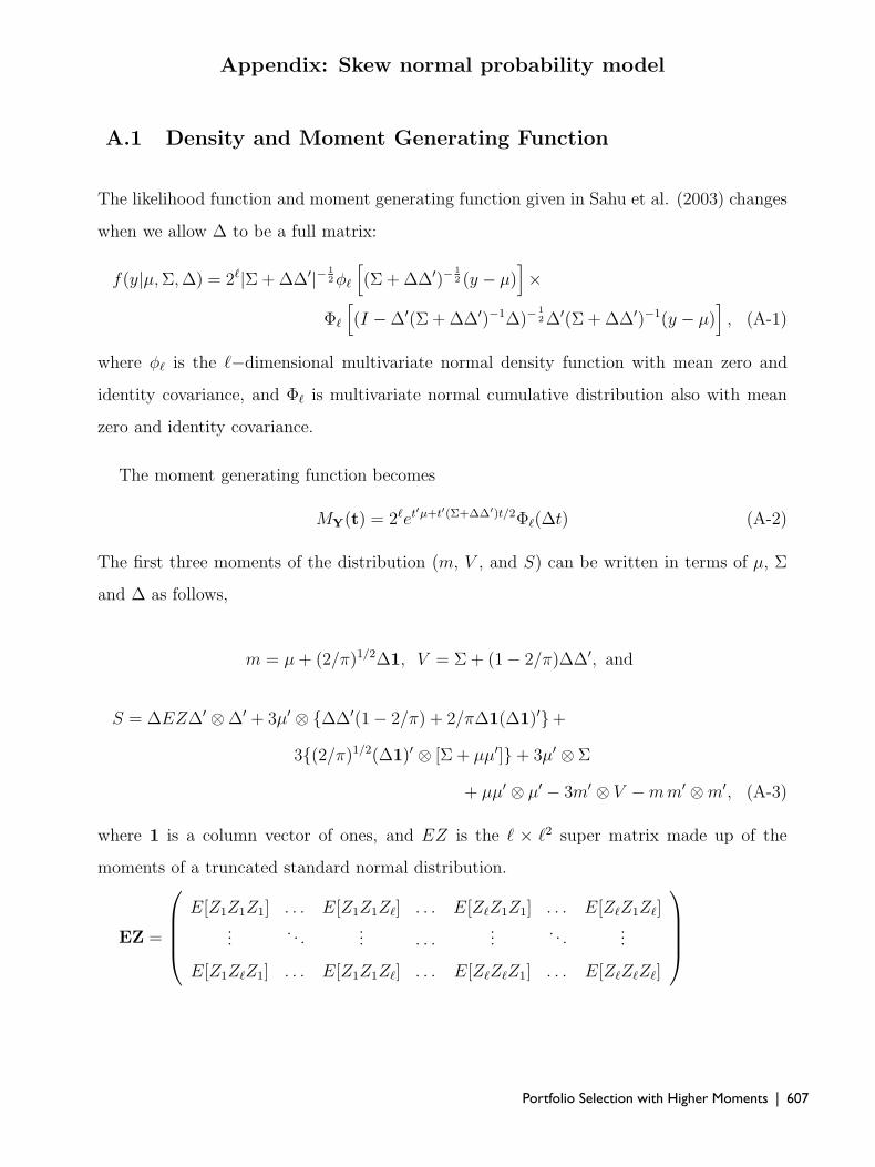
Appendix: Skew normal probability model

A.1 Density and Moment Generating Function

The likelihood function and moment generating function given in Sahu et al. (2003) changes

when we allow Δ to be a full matrix:

f(y|μ, Σ, Δ) = 2�|Σ + ΔΔ′|− 12 φ�

[(Σ + ΔΔ′)−

12 (y − μ)

]×

Φ�

[(I − Δ′(Σ + ΔΔ′)−1Δ)−

12 Δ′(Σ + ΔΔ′)−1(y − μ)

], (A-1)

where φ� is the �−dimensional multivariate normal density function with mean zero and

identity covariance, and Φ� is multivariate normal cumulative distribution also with mean

zero and identity covariance.

The moment generating function becomes

MY(t) = 2�et′μ+t′(Σ+ΔΔ′)t/2Φ�(Δt) (A-2)

The first three moments of the distribution (m, V , and S) can be written in terms of μ, Σ

and Δ as follows,

m = μ + (2/π)1/2Δ1, V = Σ + (1 − 2/π)ΔΔ′, and

S = ΔEZΔ′ ⊗ Δ′ + 3μ′ ⊗ {ΔΔ′(1 − 2/π) + 2/πΔ1(Δ1)′}+

3{(2/π)1/2(Δ1)′ ⊗ [Σ + μμ′]} + 3μ′ ⊗ Σ

+ μμ′ ⊗ μ′ − 3m′ ⊗ V − m m′ ⊗ m′, (A-3)

where 1 is a column vector of ones, and EZ is the � × �2 super matrix made up of the

moments of a truncated standard normal distribution.

EZ =

⎛⎜⎜⎜⎝

E[Z1Z1Z1] . . . E[Z1Z1Z�] . . . E[Z�Z1Z1] . . . E[Z�Z1Z�]...

. . .... . . .

.... . .

...

E[Z1Z�Z1] . . . E[Z1Z1Z�] . . . E[Z�Z�Z1] . . . E[Z�Z�Z�]

⎞⎟⎟⎟⎠


Where E[Zi] =√

2/π, E[Z2i ] = 1, and E[Z3

i ] =√

8/π. Since the Zi’s are independent,

E[Z2i Zj] = E[Z2

i ]E[Zj ] =√

2/π, and E[ZiZjZk] = E[Zi]E[Zj ]E[Zk] = (2/π)3/2 for any i, j,

and k.

A.2 First Three Moments of a Linear Combination

Assume X ∼ SN(μ, Σ, Δ) and a set of constant portfolio weights ω = (ω1, . . . , ω�)′, the first

three moments of ω′X are as follows

E(ω′X) = ω′m

V ar(ω′X) = ω′ V ω

Skew(ω′X) = ω′ S ω ⊗ ω,

where m, V and S are given above.

A.3 Levy Stable Skew Normal

When there is a Zi for each observation xi, the moment generating function readily shows

that the skew normal distributions of Sahu et al. (2003) and Azzalini and Dalla Valle (1996)

are not Levy stable. If, however, the latent variables Z are restricted to be time invariant,

i.e. a single Z for all of the observations, then both models are Levy stable. In addition, the

Azzalini and Dalla Valle (1996) model maintains the property that the distribution of the

portfolio is also skew normal.


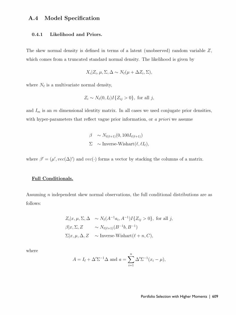
A.4 Model Specification

0.4.1 Likelihood and Priors.

The skew normal density is defined in terms of a latent (unobserved) random variable Z,

which comes from a truncated standard normal density. The likelihood is given by

Xi|Zi, μ, Σ, Δ ∼ N�(μ + ΔZi, Σ),

where N� is a multivariate normal density,

Zi ∼ N�(0, I�)I{Zij > 0}, for all j,

and Im is an m dimensional identity matrix. In all cases we used conjugate prior densities,

with hyper-parameters that reflect vague prior information, or a priori we assume

β ∼ N�(�+1)(0, 100I�(�+1))

Σ ∼ Inverse-Wishart(�, �I�),

where β ′ = (μ′, vec(Δ)′) and vec(·) forms a vector by stacking the columns of a matrix.

Full Conditionals.

Assuming n independent skew normal observations, the full conditional distributions are as

follows:

Zi|x, μ, Σ, Δ ∼ N�(A−1ai, A

−1)I{Zij > 0}, for all j,

β|x, Σ, Z ∼ N�(�+1)(B−1b, B−1)

Σ|x, μ, Δ, Z ∼ Inverse-Wishart(� + n, C),

where

A = I� + Δ′Σ−1Δ and a =n∑

i=1

Δ′Σ−1(xi − μ),


B =

n∑i=1

y′iΣ−1yi +

1

100I�(�+1) and b =

n∑i=1

yiΣ−1xi,

C =

n∑i=1

(xi − (μ + ΔZi))(xi − (μ + ΔZi))′ + �I�,

where yi = (I�, Z′i ⊗ I�).

A.5 Estimation Using the Slice Sampler

The slice sampler introduces an auxiliary variable, which we will call u, in such a way that

the draws from both the desired variable and the auxiliary variable can be obtained by

drawing from appropriate uniform densities, for more details see Damien, Wakefield, and

Walker (1999). To illustrate, assume that we want to sample from the following density,

f (x) ∝ exp

{− 1

2σ2(x − μ)2

}I {x ≥ 0} , (A-4)

where I{·} is an indicator function. We proceed by introducing an auxiliary variable u and

form the following joint density,

f (x, u) ∝ I

{u ≤ exp

{− 1

2σ2(x − μ)2

}I {x ≥ 0}

}. (A-5)

It is easy to see that based on (A-5), the marginal density of x is given by (A-4) and that

the conditional density of u given x is a uniform density, or

f (u|x) ∝ I

{u ≤ exp

{− 1

2σ2(x − μ)2

}}.

With a little more work, it is straightforward to see that the conditional density of x given

u is also uniform, or

f (x|u) ∝ I{

max(0, μ −

√−2σ2log(u)

)≤ x ≤ μ +

√−2σ2log(u)

}.

Samples from x can then be easily obtained by iteratively sampling from u conditional on x

and then from x conditional on u.


Density Estimate for Cisco

-0.2 -0.1 0.0 0.1 0.2 0.3

02

46

810

Density Estimate for GE

-0.10 -0.05 0.0 0.05 0.10 0.15

05

1015

20

Figure 1: This figure contains univariate estimates for Cisco Systems and General Electricdaily stock returns from April 1996 to March 2002. The solid lines represents the kernel den-sity estimate, while the dotted lines are the normal density with sample mean and variance.In one dimension the normal distribution closely matches the returns for these two stocks.


-0.10 -0.05 0.00 0.05 0.10

General Electric

-0.1

0.0

0.1

0.2

Cis

co S

yste

ms

Normal

Figure 2: This figure contains a bivariate normal estimate for Cisco Systems and GeneralElectric daily stock returns from April 1996 to March 2002. The plot is a bivariate nor-mal with sample mean and covariance. The scatter points are the actual data. Unlikein one dimension, in two dimensions the normal distribution does not closely match thesejoint returns. The actual returns exhibit coskewness and much fatter tails than the normalapproximation.


w

Mean:

GE

vs.

Luce

nt

0.0 0.2 0.4 0.6 0.8 1.0

0.0

004

0.0

007

w

Mean:

Sun v

s. C

isco

0.0 0.2 0.4 0.6 0.8 1.0

0.0

0140

0.0

0150

w

Mean:

GE

vs.

Cis

co

0.0 0.2 0.4 0.6 0.8 1.0

0.0

010

0.0

013

w

Variance

: G

E v

s. L

uce

nt

0.0 0.2 0.4 0.6 0.8 1.0

0.0

20

0.0

30

w

Variance

: S

un v

s. C

isco

0.0 0.2 0.4 0.6 0.8 1.0

0.0

34

0.0

37

w

Variance

: G

E v

s. C

isco

0.0 0.2 0.4 0.6 0.8 1.0

0.0

20

0.0

30

w

Ske

wness

: G

E v

s. L

uce

nt

0.0 0.2 0.4 0.6 0.8 1.0

-0.8

-0.2

0.2

w

Ske

wness

: S

un v

s. C

isco

0.0 0.2 0.4 0.6 0.8 1.0

0.6

80.7

20.7

6

w

Ske

wness

: G

E v

s. C

isco

0.0 0.2 0.4 0.6 0.8 1.0

0.4

50.5

50.6

5

Skewness:

Variance:

Mean:

Figure 3: This figure contains plots of the mean, variance and skewness of portfolios con-sisting of two assets. Daily returns from April 1996 to March 2002 for General Electric andLucent Technologies, Sun Microsystems and Cisco Systems, and General Electric and CiscoSystems are considered. The top row has the mean of the portfolio (equal to the linearcombination of the asset means) as the weight of the first asset varies from 0 to 1. Thesolid line in the plots in the second row represents the linear combination of the variancesof the assets, while the dotted line represents the variance of portfolios (variance of linearcombination). The variance of the portfolio is alway less or equal to the variance of thelinear combination. The solid line in the third row of plots is the linear combination ofthe skewness of the two assets in the portfolio, and the dotted line is the skewness of theportfolio. The skewness of the portfolio does not dominate, nor is dominated by the linearcombination of the skewness. Selecting a portfolio based solely on minimum variance couldlead to a portfolio with minimum skewness as well (see GE vs. Cisco).


Figure 4: This figure shows the space of possible portfolios based on historical parameterestimates from the daily returns of General Electric, Lucent Technologies, Cisco Systems,and Sun Microsystems from April 1996 to March 2002. The top left plot is the mean-standard deviation space, the top right plot is the mean verses the cubed-root of skewness.The bottom left plot is the standard deviation verses the cubed-root of skewness, and thebottom right plot is a three dimensional plot of the mean, standard deviation and cubed-root of skewness. In all plots that contain the skewness there is a sparse region where theskewness is zero.


Figure 5: This figure shows the mean-variance space of possible portfolios based on his-torical parameter estimates from the daily returns of General Electric, Lucent Technolo-gies, Cisco Systems, and Sun Microsystems from April 1996 to March 2002. The port-folios are shaded according to the utility associated with each. In the left plot the util-ity function is E[upred(ω)] = ω′mp − 0.5 ω′ Vp ω, which is a linear function of the firsttwo moments. The maximum utility is obtained by a portfolio on the frontier and ismarked by a ‘+’. The plot on the right is shaded according the the utility functionE[upred(ω)] = ω′mp − 0.5 ω′ Vp ω + 0.5 ω′ Sp ω ⊗ ω, which is a linear function of the firstthree moments. The maximum utility is obtained by a portfolio on the frontier and ismarked by a ‘+’.

About the Author | 617

About the Author

P rofessor Sharath M. Sury is the Dean’s Executive Professor of Finance at Santa Clara University and an Adjunct Professor of Economics at the University of California, where he teaches investment theory, corporate fi nance, and applied portfolio management. He

is the recipient of numerous teaching awards, including the DePaul University’s Seiden Award (awarded to the top member of the adjunct faculty) and Santa Clara University’s ACE Outstanding Faculty Award.

Professor Sury is also the founder and Chairman of the Board of the Santa Clara Initiative for Financial Innovation & Risk Management (SCIFIRM)—a forum that brings together the most innovative scholars in fi nance to solve problems in risk management; and serves as an Executive Advisory Board Member of the University of California’s proposed School of Management in Silicon Valley, the Arditti Center for Risk Management in Chicago, and the UCSC Center for International Economics.

In addition, Professor Sury has served as a trusted adviser to some of the nation’s wealthiest fam-ily groups and private organizations. Prior to retiring from the investment management industry, Professor Sury organized and led a nationally ranked multi-billion dollar wealth management fi rm (according to Wealth Manager Magazine, Financial Advisor Magazine, and the Bloomberg Wealth Manager Survey) and a highly respected institutional broker dealer organization. Over the years, his professional investment R&D teams—comprised of researchers with Ph.D.’s and other advanced degrees—have developed state-of-the-art techniques and strategies for client-optimized portfolio management.

In the 1990s, he also built and led one of the most successful and fastest growing wealth man-agement practices as a Vice President at Goldman, Sachs & Co., where he advised a niche group of ultra-wealthy clients representing several billion dollars in investment assets spanning equities, fi xed income, and alternative investments. During his tenure at Goldman Sachs, Professor Sury also taught several classes of incoming Goldman Sachs Financial Analysts on topics ranging from portfolio analysis to fi nancial accounting.

As an internationally recognized expert in the fi elds of portfolio theory and risk budgeting, Professor Sury is a frequently invited speaker at various prominent venues, including for the AIMR-CFA Institute, Opal Investment Summits, Financial Research Associates, FinanceIQ, ME Wealth Management Summits, Terrapin Private Banking Global India (Chair), the University of Chicago, DePaul University, and Santa Clara University. His research on the optimal integration of traditional and alternative (hedge fund) investments has been featured in a number of international presentations and his published metric, “Th e Alpha Cost Index (ACI),” is widely hailed as a technique for assessing the value of active managers.

Professor Sury had previously served in special advisory and enforcement capacities for both Federal/local government agencies and also held highly technical positions with International


Business Machines Corp. (IBM), Lockheed Missiles & Space Co. (C3I & SSD), and the MCC R&D Consortium. For his achievements in these roles, he has been highlighted in the media and awarded a variety of honors, among them the prestigious IBM Austin Excellence Award, Lockheed’s Space Systems Division Commendation, and the SCC District Attorney’s Letter for serving in one of the nation’s fi rst high technology crime/economic crime units.

Professor Sury received his MBA (High Honors) in Finance & Statistics from the University of Chicago, Graduate School of Business. He received his undergraduate degree in Economics (High Honors and Phi Beta Kappa) from the University of California, where he also held teach-ing assistantships in Macroeconomic Th eory & Statistical Analysis. In 2003, Professor Sury was featured in Crain’s Chicago Business “40 Under 40: Chicago’s Rising Stars,” for his professional accomplishments.

On a personal note, Professor Sury enjoys giving back to the community, through such eff orts as Junior Achievement, Habitat for Humanity, Starlight Starbright Children’s Foundation, and the South Shore Drill Team. He has also served on the Board of Directors of the Medical Research Institute Council of Children’s Memorial Hospital, and the Chicago GSB CEO Roundtable. Based in part on his experience in law enforcement (criminal investigation), he currently serves on the Santa Clara Co. Sheriff ’s Advisory Board and the Executive Committee of the San Jose Police Offi cer Association’s Charitable Foundation.

portfolio selection with higher moments - duke's fuqua ...charvey/research/... · portfolio...

Documents