Clemson UniversityTigerPrints

All Theses Theses

5-2011

POSE ESTIMATION FOR ROBOTICDISASSEMBLY USING RANSAC WITH LINEFEATURESShyam sundar Aswadha narayananClemson University, an.shyamsundar@yahoo.com

Follow this and additional works at: https://tigerprints.clemson.edu/all_theses

Part of the Robotics Commons

This Thesis is brought to you for free and open access by the Theses at TigerPrints. It has been accepted for inclusion in All Theses by an authorizedadministrator of TigerPrints. For more information, please contact kokeefe@clemson.edu.

Recommended CitationAswadha narayanan, Shyam sundar, "POSE ESTIMATION FOR ROBOTIC DISASSEMBLY USING RANSAC WITH LINEFEATURES" (2011). All Theses. 1126.https://tigerprints.clemson.edu/all_theses/1126

POSE ESTIMATIO FOR ROBOTIC DISASSEMBLY USIG RASAC WITH LIE

FEATURES

A Thesis

Presented to

the Graduate School of

Clemson University

In Partial Fulfillment

of the Requirements for the Degree

Master of Science

Electrical Engineering

by

Aswadha Narayanan Shyam Sundar

May 2011

Accepted by:

Dr. Richard E. Groff, Committee Chair

Dr. Stanley T. Birchfield

Dr. Dennis E. Stevenson

ii

ABSTRACT

In this thesis, a new technique to recognize and estimate the pose of a given 3-D object

from a single real image provided known prior knowledge of its approximate structure is

proposed. Metrics to evaluate the correctness of a calculated pose are presented and analyzed.

The traditional and the more recent approaches used in solving this problem are explored and the

various methodologies adopted are discussed.

The first step in disassembling a given assembly from its image is to recognize the

attitude and translation of each of its constituent components – a fundamental problem which is

being addressed in this work. The proposed algorithm does not depend on uniquely identifiable

3D model surface features for its operation – this makes it ideally suited for object recognition

for assemblies. The algorithm works well even for low-resolution occluded object images taken

under variable illumination conditions and heavy shadows and performs markedly better when

these factors are removed.

The algorithm uses a combination of various computer vision concepts such as

segmentation, corner detection and camera calibration, and subsequently adopts a line-based

object pose estimation technique (originally based on the RANSAC algorithm) to settle on the

best pose estimate. The novelty of the proposed technique lies in the specific way in which the

poses are evaluated in the RANSAC-like algorithm. In particular, line-based pose evaluation is

adopted where the line chamfer image is used to evaluate the error distance between the

projected model line and the image edges. The correctness of the computed pose is determined

iii

based on the number of line matches computed using this error distance. As opposed to the

RANSAC algorithm where the search process is pseudo-random, we do an exhaustive pose

search instead. Techniques to reduce the search space by a large amount are discussed and

implemented.

The algorithm was used to estimate the pose of 28 objects in 22 images, where some

images contain multiple objects. The algorithm has been found to work with a 3-D mismatch

error of less than 2.5cm in 90% of the cases and less than 1cm error in 53% of the cases in the

dataset used.

iv

DEDICATION

To my mom who laid the very foundation of my education

To my dad who helped me build on it

v

ACKNOWLEDGEMENTS

I like view this work as a crystallized version of numerous ideas inspired by a lot of

people around me, directly and indirectly; wittingly and unwittingly. It just wouldn’t have

become what it is now without their help and encouragement.

First of all, I thank my advisor, Dr. Richard Groff for the gargantuan amount of time and

effort he has taken in walking me through this long journey involving multitudes of equations,

algorithms and programming techniques. In retrospect, the work would have remained just

another unfulfilled effort without his crucial inputs.

I must thank my friends, particularly Vinay Gidla, Vidya Murali, Harshwardhan Karve,

Aditya Sriram, Varun Prabhu and Nivedhitha Giri who provided fuel for extremely insightful

discussions on topics ranging from Human psychology, Robotics, Artificial Intelligence and

Theology which has had its own impact on my way of thinking, and consequently my research

work. I must also thank them for putting up with my occasional bouts of insanity while I used to

be engrossed in solving a sub-problem towards this work, which I have come to accept as an

endemic part of a graduate student research life.

Most importantly, I thank my parents, especially my mom who goaded me to never give

up on any problem, be it research or otherwise and provided me all the moral support I acutely

required over this long and arduous journey. It was she who instilled in me the belief that every

vi

problem has a definite solution and that one could find it by looking for it hard enough. I know

that I cannot repay even a fraction of what I really owe her.

vii

TABLE OF CONTENTS

Page

TITLE PAGE……………………………………………………………………………………...i

ABSTRACT…………………………………………………………………………………........ii

DEDICATION……………………………………………………………………………….......iv

ACKNOWLEDGEMENTS………………………………………………………………………v

LIST OF FIGURES……………………………………………………………………………..viii

CHAPTER

I. INTRODUCTION…………………………………………………………….……....1

I. THE PROBLEM AND MOTIVATION……….………….…………………..1

II. LITERATURE SURVEY…………….……………………………………….6

II. THE RANSAC WITH LINE FEATURES ALGORITHM…………....……..….…..14

I. BACKGROUND…………………………………………………………….14

I. PERSPECTIVE TRANSFORMATION…………………………………....14

II. POSE ESTIMATION WITH KNOWN CORRESPONDENCES….…..…..19

III. IMAGE PROCESSING AND 3D MODELING………..…….……………30

II. ALGORITHM……………………………………………………..….….…..34

III. RESULTS AND DISCUSSION…………………………….………..…….………..42

I. DATA USED AND METHODOLOGIES…………..………………..……..42

II. RESULTS………………………………,…..……………………………….45

III. DISCUSSION……………………………………………..……….……..….49

IV. CONCLUSIONS AND FUTURE WORK………………………..…….……….…..55

V. REFERENCES….…………..………………………………………………….…....59

viii

LIST OF FIGURES

Figure Page

2.1 Pinhole camera model…………………………………………………………...15

2.2 Representation of the various coordinate systems………………………………16

2.3 Camera coordinate system………………………………………………………17

2.4 Rotation and translation of a triangle in space…………………………………..20

2.5 Perspective three-point problem………………………………………………...22

2.6 Representation of a 3D model………………………………………………......32

2.7 Segmented object…………………………………………………………….….35

2.8 Edge image………………………………………………………………….…..36

2.9 Chamfer edge image……………………………………………………….........36

2.10 Prominent corners in the segmented region…………………………….….........37

2.11 Computing Average and Total Line Mismatch Error………………….….…….39

2.12 Global and local ratios used in the algorithm…..…………………………....…..41

ix

List of Figures (Continued)

Figure Page

3.1 True and estimated poses of the red cuboid ….…………………………………...47

3.2 True and estimated poses of the green cuboid .…………………………………...48

3.3 3D Mismatch Error Performance plot…………….…………………………….…48

3.4 Translation Mismatch Error Performance plot……………………………………49

1

CHAPTER ONE

INTRODUCTION

1.1 THE PROBLEM AND MOTIVATION

Much progress has been made in the process of automating assembly processes in the

manufacturing industry. In contrast, the reverse process of automated disassembly is currently

plagued by numerous practical difficulties and remains an unsolved real-world problem.

Products that go through the disassembly process are most likely to be recycled and one could

generally expect random deformations in them. Thus, any algorithm that is tailored for

disassembly must be robust to minor object deformations.

Robotic disassembly of used products is increasingly relevant due to legal requirements

placed upon manufacturers to recycle their products. However, disassembly of end-of-life

products has traditionally been a manual process owing to the numerous technical difficulties

associated with it. The deformed shape of waste products constitutes a common obstacle and

poses a considerable challenge to the application of robotic arms in this process. A natural

consequence of the difficulties associated with this process has been the adoption of recycling

methodologies without any kind of inbuilt intelligence. Such recycling techniques usually

involve the use of shredders, smelters and similar equipment that “blindly” convert a bunch of

scrap into a heterogeneous mass of recycled material, losing much of the potential initial worth

of the products.

2

In addition to this, a task like recycling of electronic waste usually entails dealing with

toxic, hazardous substances. These factors combined with the persistent need for manual labor in

this industry leads to a situation where the cost of recycling a used product often exceeds the cost

of manufacturing a new, similar product. Extensive studies on the associated cost analysis have

been done earlier by Yuksel and Baylakoglu [1]. In a nutshell, their study concluded that a

specific, optimized disassembly plan for a given product would be economically feasible. Our

work essentially constitutes an attempt to help generalize the disassembly process for any given

assembly. We will proceed to discuss the various traditional approaches adopted towards solving

the disassembly problem and subsequently transition to the discussion on pose estimation in the

following few paragraphs.

The earliest approaches which aimed to solve the disassembly problem were almost

exclusively based on Maximum Likelihood estimation (ML estimation) and Maximum a

posteriori Probability estimation (MAP estimation), and have been used to estimate the relative

positions of parts in a known assembly using an image. A typical ML approach is by Sanderson

[2], where the assemblability of a set of assembly components in a configuration is explored in

terms of ML-based constraint clearance in their vicinity. This measure of assemblability was

incorporated into an AND/OR graph described by Mello and Sanderson [3] to make a decision

on the sequence of steps for the disassembly procedure for an object with known construction.

The more noise-robust MAP estimate can be looked at as a variant of the Maximum

Likelihood estimate in the sense that here we make use of a known a posteriori object probability

distribution along with the data used for maximum likelihood estimation. Tretter [4] had earlier

3

used a fast multi-scale technique to compute the Sequential MAP (SMAP) of the unknown

position, scale factor and 2-D rotation for each subassembly. This technique affords additional

accuracy over the MAP estimate owing to the search through multiple resolution levels. The

drawback with the estimation techniques is that they are extremely application-specific in terms

of their success and prior knowledge of the associated assembly structure is needed for reliable

pose estimation.

It is imperative to have a good way of representing assemblies prior to thinking about

their disassembly. Sagerer [5] had proposed the use of context free grammars to represent

assemblies. The core idea behind this representation is the reusability of the mating properties of

the subassemblies. Each assembly can be looked at as a valid sentence constructed using certain

predefined rules. These rules are a direct consequence of the configuration of the subassemblies.

Valid sentences (an assembly, in this case) are a byproduct of substitution of a given rule in other

rules in myriad ways. This is explained through a specific example in [6].

As noted earlier, there are well developed techniques to represent assemblies in terms of

their subassemblies. Mello and Tretter’s work [3][4] on assemblability and assembly inspection

shows that if the components and configuration of an assembly are known beforehand, the

problem of optimal disassembly breaks down into a simple graph search. There are standard

techniques such as the Ant Colony optimization which is used for evaluating the sequence of

disassembly operations with an aim of arriving at the most optimal solution and has been

described by Shan [7].

4

However, these techniques can be applied to a practical assembly at hand for an

automated disassembly process only if the individual subassemblies are first recognized and their

poses computed. This would mean that one could then, for instance, construct the AND/OR

assembly graph using these poses straightaway and proceed to using the Ant-colony optimization

algorithm mentioned earlier. In other words, to actuate the process of disassembly of a real

assembly given its image, one needs to first find out the location and orientation of each of the

assembly components in order for a robot to be able to take them apart.

As mentioned earlier, most assembly objects in line for recycling need not necessarily, in

practice, conform to the exact dimensions as specified by the prior object attribute information.

Pose estimation can be looked at as an Artificial Intelligence problem, the solution for which

seeks to emulate human intelligence in recognizing the position and orientation of a given object

placed amidst a cluster of connected/disconnected objects in a scene with numerous visual

constraints enumerated earlier.

Pose-estimation is an essential and a fundamental step that one must take prior to any

disassembly process planning. This is because pose-estimation helps reveal some information

about how the assembly components are oriented or interconnected in space and could

potentially help generate directions on how to actuate the disassembly process using robotic arms

or an equivalent actuator. A general disassembly algorithm is fundamentally more complex than

a generic assembly algorithm. This is because a disassembly process generally may take place in

a less structured environment without much a priori information about the constituent assembly

object components. While there has been a significant amount of work done in designing a

5

disassembly plan [3] given a graph composed of nodes of connected components, such

information might not be known in advance.

The object pose estimation problem is a partially unsolved problem with limited success

on a real image. In this research work, an algorithm that would reliably estimate the true pose of

a given object with known 3D configuration from a single image with high accuracy under

variable lighting conditions and object occlusions is proposed.

In this thesis the problem of pose estimation of known objects from a single real image

without having any prior information about known point or edge correspondences is solved.

Given the 3-D model of a specific object represented using its corners and faces we can reliably

estimate the true rotation and translation of this object in the given image despite the presence of

shadows, variable lighting conditions and occlusions. In this work, the methodologies discussed

are generally suited for a typical connected/disconnected assembly or its components. We also

present and analyze two metrics, one discrete and another continuous, each of which give an

estimate of the correctness of the calculated pose.

This thesis is organized into 5 major chapters in the following order: Introduction, The

RANSAC with Line Features, Results and Discussion, Conclusions and Future work, and

References. The first chapter, Introduction, is organized into two subdivisions: the first

describing the problem solved and the motivation behind and the second containing the literature

review involved in this research. The second chapter is divided into two parts. The first part

gives the necessary background for understanding the subsequent material in the Algorithm

6

subsection. Owing to the complex, abstract nature of pose estimation, we further divide this part

into three subdivisions: perspective transformation, pose estimation with known correspondences

and image processing and 3D modeling. The second part of the chapter on Theory, describes the

algorithm and its implementation. The third chapter presents the results and draws a contrast on

the strengths and weakness of the proposed algorithm. The penultimate chapter discusses the

potential improvements to the proposed algorithm and gives a direction for future research. The

final chapter enumerates the references used over the course of this work.

1.2 LITERATURE SURVEY

Pose estimation is the process of determining the rotation and translation of 3-D object

representation in an image with respect to a given coordinate system. Pose estimation usually

involves matching the 3-D object features onto the corresponding 2-D image features. Given the

correspondences between object and image features, rotation and translation can be computed.

However, these correspondences cannot be easily determined given just the 3-D model and the

object image and remains an unsolved problem in case of images with featureless assemblies

thus far.

Pose estimation using known correspondences is a thoroughly studied problem. The

solution to a fundamentally important solved problem within pose estimation is the Perspective

three-point problem (also known as the P3P problem) which gives us a way to solve the pose

estimation problem with known correspondences. The POSIT (Pose from Orthography and

Scaling with iterations) algorithm by Dementhon [8] utilizes known correspondences for

7

determining the object rotation and translation matrices. This algorithm first uses the POS (Pose

from Orthography) for estimating the rotation and translation matrices given a set of known

correspondences. The POSIT algorithm constitutes an improvement over the POS algorithm in

that it first utilizes the POS algorithm to obtain a deterministic solution for a good initial guess of

the pose. Subsequently, an iterative procedure to refine the obtained pose is proposed. This

algorithm, in addition to being computationally efficient, is claimed to be relatively robust to

both noise and errors in correspondence set.

Dementhon subsequently proposed an iterative algorithm called the SoftPOSIT algorithm

[9] which did not require known correspondences to match a set of 3-D model points to image

points. The SoftPOSIT algorithm alternately estimates the correspondence probabilities given the

current pose and then estimates the pose given the correspondences. This algorithm takes a set of

3-D model points and another set of 2-D image points as parameters. Note that the sets may be of

different sizes. The principal idea behind this iterative algorithm is to use a doubly stochastic

matrix, the entries of which signify correspondence weights in terms of probability densities,

over subsequent iterations to refine the point matches. This matrix is utilized in a proposed

metric to minimize the error between the set of 3-D points projected onto the image plane and

the set of corresponding 2-D image points. Later work by Dementhon utilizing line features

rather than corner features [9] [10] has been shown to produce results that are more robust to

noise. This is expected as line features contain more information than point features.

Another prominent correspondenceless pose estimation technique is the Gravitational

Pose Estimation Algorithm (GPE Algorithm) by Ugurdag [11]. This algorithm utilizes the

8

distance between the rays shooting out from the camera focus and passing through the object

features (which are taken to be corners in this algorithm’s implementation) and the image

features visible in the given object image. The idea behind the formulation of this algorithm is to

utilize appropriate force vectors from the image points that would make the object at an arbitrary

initial pose converge to its correct location using an iterative process. In each iteration, the force

vectors that act on the 3-D model points is successively refined based on the distance between

the object rays and the image features. The algorithm is assumed to have converged and

terminates when the change in pose metric between successive refinements is below a predefined

threshold. A metric based on the rays and the image points is proposed and its performance is

evaluated.

The RANSAC algorithm proposed by Fischler and Bolles [12] is by far the most relevant

piece of research that meshes most closely with our work. The RANSAC algorithm in a single

pass, assigns three random correspondences between 3-D object features (usually corners) and

the image points. The resulting correspondence problem is then solved to obtain the associated

object model point depths using the solution for the Perspective three-point problem, also known

as the P3P problem. This solution is then translated to the corresponding rotation and translation

matrices. It is to be noted that the P3P problem may have more than one valid solution. This will

be discussed again in a greater depth in the chapter 2. There has been a scarcity of robust metrics

tested on real data that could be interfaced to the RANSAC algorithm to test the goodness of an

estimated pose. This is exactly where our work fits into the bigger picture. We utilize the

solution to the P3P problem for each set of possible 3-D model to 2-D image three-point

correspondences and deterministically calculate the pose of the object. The estimated pose is

9

now projected onto the image plane and its appropriateness for the image at hand is evaluated

using an object-edge based metric which will be proposed in the next chapter.

The SoftPOSIT algorithm utilizing only the point features has been found to work well

only on synthetic images when the initial guesses are relatively close. When the object’s initial

pose is kept at an arbitrary location in the presence of stray points, the algorithm converges to a

false pose most of the time. The SoftPOSIT algorithm using lines is relatively more robust to the

presence of false features. However, this algorithm requires a good initial guess for a given pose

hypothesis in order for it to converge to the true object position. To overcome this problem, this

algorithm utilizes a large number of poses and applies the iterative convergence algorithm to

each of the cases. The best fit among the converged poses is the one that minimizes a predefined

objective function. However, this algorithm has been tested only using accurate 3-D models and

images with sharp, distinct features. Even under such circumstances, the resulting average pose

estimation error computed is found to average about 20-30 degree rotation from the original

pose.

The Gravitational Pose estimation suffers from similar disadvantages. The GPE, like the

SoftPOSIT needs a decent initial guess for guaranteed convergence to the right pose. Further,

this algorithm has been only tested on 2-D scenes viewed in 3-D and without the presence of

additional noise.

The RANSAC algorithm, in its current state requires to be interfaced with techniques

from computer vision and a good metric for estimating and measuring the goodness of a pose.

10

The proposed RANSAC-based algorithm works in conjunction with both line features and a

plethora of Computer Vision techniques. We realize that this two-pronged approach is absolutely

essential to recognizing the true object pose from real images taken under heavy clutter,

occlusions and heavily varying lighting conditions. Further, this approach would enable us to

detect the pose of the object in the image even if its 3-D model is does not match exactly with the

actual object model in the image.

The fundamental difference between the line-based SoftPOSIT algorithm and the

RANSAC-based algorithm we propose lies in the area of application. The line-based SoftPOSIT

algorithm, by its very formulation, is more suited to pose estimation in a natural, cluttered scene.

On the other hand, we try and solve the pose estimation problem for assemblies. This makes the

two algorithms very different from each other as each is designed and optimized for the

application it was intended for and would be inappropriate for direct comparison. SoftPOSIT

with lines is more suited to scenes with an abundance of line features while our algorithm is

adapted for images with very few features present. Though theoretically our algorithm would

give results that are comparable or better than SoftPOSIT owing to its reliance on an exhaustive

search, a major drawback would be the high computation time involved.

The other pose estimation techniques that have been proposed earlier are the genetic

algorithm based EvoPose and approaches based on Neural Networks and Lookup tables.

There has been much prior work done on Genetic Algorithm based pose estimation.

Toyama’s work on Model based pose estimation [13] involved searching for the most probable

11

poses through a six-dimensional space where the best one of the lot was picked using a fitness

criterion. Kayanuma [14] had used a 3-D object model with features to determine the object pose

through a single image. The pose search is done using a genetic algorithm and the number of

model-image feature matches determines the fitness of the pose.

Another notable genetic algorithm based technique is the EvoPose [15]. The EvoPose is

similar in operation to Toyama’s method in that it searches through a six-parameter space;

however, the EvoPose relies solely on points rather than edges.

Neural Network approaches have been used in the past by Langley [22] for estimating the

pose of a Fixtureless assembly. However the results obtained using this approach is contingent

on the presence of a sufficient number of surface features and an appropriate training data set,

and has been found only moderately successful against simple assemblies.

Another computer-vision based approach for pose estimation is to have a huge dataset of

an object with known poses. The camera image at hand is then compared with each of these

images. The database image with the best match is singled out in the process and its pose is read

from the lookup table. An example of related work is by Rother [16] who used 3-D shape priors

to estimate the image appearance by projecting them down on the image plane and then

computing probability of image match. While this approach could guarantee good results without

much real-time computation, the necessity of having a large database for each object in a variety

of different environments rules out the use of such an approach in a practical scenario.

12

David Lowe’s seminal paper on SIFT [17] (Scale Invariant Feature Transform) is an

interesting place to begin work on pose estimation. The work provides us an extremely robust

way to recognize known 2-D objects in a cluttered scene containing them. Each feature is

uniquely identified using local gradient information represented in a 128-bit format. The image

features chosen are image points with distinct gradient vectors. This makes them invariant to

rotation, translation and scaling. The drawback with this technique is that it cannot be adapted

for objects with few, poor feature descriptors. Moreover, the SIFT algorithm was originally

designed to operate only on 2-D object features.

The SIFT features are relevant to pose estimation because they provide a way to obtain

scale and rotation invariant image features. They are particularly useful when the object under

consideration has plenty of distinct identifiable surface features. In such cases, the object’s pose

can be computed using pose estimation techniques utilizing known correspondences.

This technique could be extended to 3-D objects by having a picture of each face of the

object and recognizing them separately. Ambiguity arises when we have a general, rounded

object whose faces are not clearly defined. Savarese’s work [18] utilizes this idea and gets the

SIFT features of the “parts” (or faces, in the paper) of a given 3-D object. The faces are

recognized separately and a homography matrix to transform the priori images to match the

rotated images in the scene is computed. The object is viewed as a connected graph of the

images.

13

Correspondence-based pose estimation could be a viable research direction to proceed on

provided the 3-D object model has a sufficient number of distinct features that could be readily

identified from its 2-D image. This process will most likely be subject to correspondence errors

in case of a real image. To overcome this problem, Haralick [19] proposed a pose estimation

technique using known correspondences that would be robust for up to thirty percent of

correspondence mismatches. This is in contrast to the least-squares based solution provided

earlier, where such situational errors give rise to meaningless solutions. As stated earlier, this

doesn’t prove particularly useful in our work as we deal with images having a paucity of feature

points.

14

CHAPTER TWO

THE RANSAC WITH LINE FEATURES ALGORITHM

2.1 BACKGROUND

2.1.1 PERSPECTIVE PROJECTION

The process of capturing the image of a 3D model is essentially a linear mapping of the

3D model points in the world onto a 2D image plane. This transformation, also known as

perspective projection is crucial for understanding pose estimation.

For real images shot in practical scenes, a common approximate model is the pinhole

camera model, which models the camera as a perspective projection. This model describes the

mathematical relationship between observed 3D point in the scene and the corresponding 2D

image point. In this model, the camera aperture is assumed to be a single point with multiple rays

converging on it from various directions. An inverted image of the scene is formed on the plane

containing the camera focus. Equivalently, one could think of the rays converging directly at the

camera focus, with the image being formed at the plane passing through the aperture. The

perpendicular distance of this plane from the focus is equal to the focal length of the camera.

15

Figure 2.1: Pinhole camera model

In Figure 2.1, I is the point of intersection of the ray OR with the image plane. The focal

length is f and the observed model point is R.

By triangle similarity of triangles OIP and ORL,

xu=f

z and

yv=f

z

Thus, we see that the intersection coordinates are just the scaled versions of the normalized

world coordinates. This leads us to the principal idea behind camera calibration.

For mapping a 3-D model observed using an image captured using a pinhole camera onto

the corresponding 2-D image plane, one of the first steps one must take is to calibrate the

camera. Camera calibration matrix describes the transformation between the 3-D points

measured in the camera coordinate system and the 2-D coordinates using the image coordinate

system.

16

Figure 2.2 shows the different coordinate systems we use in camera calibration. Oc is

origin of the camera coordinate system. Its corresponding Z-axis, Zc is perpendicular to the

image plane and passes through the principal point of the image, (u0, v0). Xc and Yc are chosen

parallel to the image coordinate axis Xi and Yi as shown in the figure. Xo, Yo and Zo refer to the

object coordinate system which is assumed to be attached to the object at hand. They are useful

for expressing object dimensions in a more lucid fashion.

Figure 2.2: Representation of the various coordinate systems

Ow is the center of the world coordinate system with axes Xw , Yw and Zw. It is sometimes

used since it is more natural to think about the rotation and translation of an object with respect

to a fixed world coordinate system that is usually somewhere in the vicinity of the object as

opposed to the camera coordinate system. This is because the camera coordinate system changes

for different camera views and would not, consequently, provide a standard reference frame.

17

The camera calibration matrix, C, relates the 3-D model point, [Xi Yi Zi]T, measured with

respect to the camera coordinate system with a point on the ray [xi yi zi]T starting from the camera

focus and passing through the object model point whose position is measured with respect to the

camera coordinate system with the image coordinate metric.

0

00

0 0 1

i u i

i v i

i i

x u X

y v Y

z Z

α γα

=

(2.1)

Equation 2.1 represents perspective projection of the 3-D model point onto the image plane. Camera

calibration is the process of finding the perspective projection matrix (or camera calibration matrix) for a

specific camera.

Figure 2.3: Camera coordinate system

18

Here, ∝u is the scaling factor along the X-axis and ∝v is the scaling factor along the Y-

axis. γ is the image skew factor and [u0 v0]T is the principal point and generally lies at the

geometric center of the image. This point specifies the translation of the intersection point

between Zc and the image plane with respect to the image coordinate system. If [u0 v0]T were

made equal to [0 0]T, it would imply that all the image coordinate measurements were made from

the image coordinate system with an origin translated to the center of the image.

For a normal camera without distortions, the skew factor γ is generally negligible and can

be taken to be 0. ∝u and ∝v are generally in practice, equal to the focal length of the pinhole

camera (A generalization which we do not assume in our case) and can be thought of the pixel

scaling factors along the X and Y axes respectively. The equation 2.1 then becomes:

0

0

0

0

0 0 1

i u i

i v i

i i

x u X

y v Y

z Z

αα

=

(2.2)

Since [xi yi zi]T represents a point along a ray with coordinates measured with respect to

the camera coordinates in image coordinate metric, we could obtain the actual image coordinates

as measured from the screen by normalizing this vector, that is dividing xi, yi and zi by zi.

The actual image coordinates of the point is [xi/zi yi/zi 1]T.

Put briefly, camera calibration is the process of finding the characteristic transformation

matrix that transforms 3-D object points into the corresponding image points. One of the most

popular techniques for calibrating a given camera is Zhang’s method [20]. The camera

19

calibration matrix when multiplied with the 3-D object coordinates results in a point along the

ray passing through the camera focus and the 3-D object point. On normalizing the output vector

by dividing each element in the vector by the Z-value, we can get the actual image point.

Basically, camera calibration is a tool to directly transform the points on the rays passing

through the image into the 3-D object points and vice-versa. This implies that if we associate

three image feature points with corresponding object points, we could find out the angle

subtended at the focus by each pair of the feature points. The angle subtended by any two object

model points at the camera focus is computed as the cosine inverse of the dot-product of the

vectors shooting out from the focus in the directions of the model points. Due to the image point

and 3-D object point association, we know the true distances between the selected image feature

points. Thus, the problem of pose estimation reduces to solving the perspective three-point

problem which we shall discuss soon.

2.1.2 POSE ESTIMATION USING KNOWN CORRESPONDENCES

There are several methods of estimating the object pose, given correspondences between

image points and points two of which will be presented here. The first method is based on the

solution to the P3P problem. The P3P solution is used in the RANSAC algorithm while the

second method used in computing the “true” pose of objects in the data set in Chapter 3.

We will now discuss the pose estimation using the solution to the perspective three-point

problem. The various coordinate systems have already been described using Figures 2.2 and 2.3.

20

We now look at the problem of mapping a model triangle, originally in 3-D space at a known

position and orientation into another an observed location through a rotation and translation.

Figure 2.4 shows the triangle ABC initially present in 3-D model being rotated and

translated to a position to match with the visible triangle in the image. When this rotation and

translation for a particular triangle in the 3-D model is found to match well with a triangle seen

in image, we can take that rotation and translation to be the pose of the object visible in the

image computed with respect to the camera coordinate system. In general, a good matching

criterion would be that all the visible corner feature points that are present in the 3-D model be

regenerated using the pose transformation matrix which ideally matches with the image corner

features.

Figure 2.4: Rotation and translation of a triangle in space

21

The rotation and transformation of the triangle described earlier is found using the

solution to the perspective three-point problem, or simply, the P3P problem. Let us now look at

its problem statement and solution in greater detail.

Assume we are looking at a triangle of known dimensions using a pinhole camera. In our

problem, we look at the 3-D object as being made up of triangles, one of which is under current

consideration. As discussed earlier, camera calibration helps compute the angle subtended to the

focus by the 3-D object points visible in the image as corner features.

The perspective 3-point problem deals with the problem of finding out the actual

distances from the focus to each of the object points represented by the triangle provided the

triangle dimensions and the angle subtended at the focus is known. Once these distances are

known, we can compute the rotation and translation of this triangle on the object with respect to

a predefined initial position with respect to the camera focus assumed originally. The perspective

three-point problem can have a maximum of eight real solutions, out of which a maximum of

four can be positive. This solution is presented in the appendix of [12].

Figure 2.5 shows the diagram describing the perspective three-point problem. O is the

focus of the camera looking at the triangle ABC with sides Rab, Rac and Rbc. The points A, B and

C have the depths a, b, c with angles between OA, OB and OC rays shooting from the camera

represented as θ1, θ2 and θ3.

22

Figure 2.5: Perspective three-point problem

By cosine formula,

2 2 212 cos( )abR a b ab θ= + −

2 2 222 cos( )acR a c ac θ= + −

2 2 232 cos( )bcR b c bc θ= + −

Let us now define variables K1, K2, G0, G1, G2, G3 and G4 as follows:

2

12

ab

ac

RK

R=

2

22

bc

ab

RK

R=

23

2 24 1 2 1 2 1 2 3( ) 4 cos ( )G K K K K K K θ= − − −

3 1 2 1 2 2 1 1 1 3 1 2 2 1 2

2 1 3

4( ) (1 )cos( ) 4 cos( )[( . ) cos( )

2 cos( ) cos( )]

G K K K K K K K K K K K

K

θ θ θθ θ

= − − − + + − +

22 2 1 1 1 2 1 2 1 2 1 2

2 21 1 2 3 2 1 2 2 1 1 2 3

[2 (1 ) cos( )] 2[ ][ ]

4 [( ) cos ( ) (1 ) cos ( ) 2 (1 )cos( )cos( )cos( )]

G K K K K K K K K K K

K K K K K K K

θ

θ θ θ θ θ

= − + + − − − +

− + − − +

1 1 2 1 2 2 1 1 1 1 2 1 2 2 3

21 2 1 2

4( ) (1 )cos( ) 4 [( )cos( )cos( )

2 cos( ) cos ( )]

G K K K K K K K K K K K

K K

θ θ θ

θ θ

= + − − + − + +

2 2 20 1 2 1 2 1 2 2( ) 4 cos ( )G K K K K K K θ= + − −

The solution to the P3P problem is obtained from the roots of the following quartic equation:

4 3 24 3 2 1 0 0G x G x G x G x G+ + + + =

Now,

212 cos( ) 1

abRa

x x θ=

− +

.b a x=

2 22

2 22

cos( ) cos ( )acR a

ya

θ θ−

= ± +

.c y a=

The a, b and c values must be verified by the cosine equations we started out with before

they can be accepted. There can be a maximum of 8 real solutions and a maximum of 4 positive

real roots.

24

The direct solution of the 3-point perspective problem yields distances rather than the

rotation and translation matrices for the pose of an object. The distances can be transformed into

the rotation and translation matrices using as follows.

Let P1, P2 and P3 be the three model points chosen from the 3-D object model initially

placed at the camera focus. The distances of the three feature points from the camera focus are

detected assuming the feature points in the image correspond to the model points. Since the

vectors from O to A, B and C are known (From the camera calibration matrix formula discussed

earlier), the 3-D position of the feature points are also known. Let us represent them by variables

P1’, P2’ and P3’.

Let us now define matrices M1 and M2 containing vectors describing the triangle object

coordinate system as follows:

[ ]1 2 1 3 1 2 1 3 1( ) ( ) ( ) ( )M P P P P P P P P= − − − × −

[ ]22 2 1 3 1 1 3 1( ' ') ( ' ') ( ' ') ( ' ')M P P P P P P P P= − − − × −

The approximate rotation matrix, Rapprox is obtained using the following equations:

2 . 1approxM R M=

12 1approxR M M −=

Rapprox is now subjected to singular value decomposition and is forced into a true rotation matrix

of determinant equal to 1 using the following two equations. If the determinant of the resulting

matrix is found to be -1 instead, the matrix is subject to scalar multiplication by -1 to make the

determinant equal to 1. Now, the rotation matrix, Rapprox is calculated as a product of the

orthogonal matrices U and VT:

25

TapproxU V RΣ =

TapproxR UV=

The corresponding translation is found using the traditional pose-transformation formula, where

P is a general point from the original pose and P’ is the transformed point after rotation and

translation:

'0 1 1

R T PP

=

1 1 1'T P RP= −

2 2 2'T P RP= −

3 3 3'T P RP= −

The translation, which must ideally have T1=T2=T3, is now subject to error minimization by

taking the average of the three vectors T1, T2 and T3.

1 2 3

3

T T TT

+ +=

We will now discuss the second pose estimation technique using sets of known

correspondences mentioned in the beginning of this section. It would be quite useful to discuss

the mathematics behind the computation of pose given a set of 3-D object points with respect to

a known world coordinate and the corresponding 2-D image points. This technique is used for

refining the estimated pose and obtaining the true pose by superimposing the estimated pose over

the image of the object under consideration. This pose estimation technique differs slightly from

the P3P pose estimation technique. In the P3P pose estimation technique, we have known

correspondences between just three model points and three image features. In contrast, in this

26

pose estimation technique, we have known correspondences between at least six image points

which are chosen manually and the associated object model points. In other words, we do not

depend on the features detected by the corner detector, on the contrary, we hand-pick the image

points corresponding to the object corners. An outline of this technique is described in [9].

Let Xi, Yi and Zi be the 3-D model coordinates with respect to the camera coordinate

system and xi and yi be the corresponding image coordinates of depth s. The relationship between

the two can be expressed as:

0

0

0 0

0 0

1 0 0 1 01

i

i u

i

i v

i

s

Xx u

Yy v

Z

αα

=

If Xi, Yi and Zi are in terms of the object coordinate system, the object rotation and

translation with respect to the camera coordinate system is given by:

1 1

0

2 2

0

3 3

0 0

0 0

1 0 0 1 01 1

i

i u

i

i v

i

s

r t Xx u

r t Yy v

r t Z

αα

=

⊙

(2.3)

Here, r1, r2 and r3 are the horizontal rows of the rotation matrix and t1, t2 and t3 are the

scalar values present in the translation vector.

27

Thus,

1

3 32

3

R x

r

R r

r

= ∈

and,

1

3 12

3

R x

t

t t

t

= ∈

From equation 2.3, multiplying by the inverse of the camera calibration matrix, C, on both sides,

we get:

[ ]1 1

3 1

1 3 11

1

i

i

i

i xix

Xx

R t YsC y C C

Z

− −

=

⊙⊙

Multiplying the inverse of the camera calibration matrix with the image coordinates yields a 3D

point [xi’ yi’ zi’]T along the ray that emanates from the camera focus and passes through the 3D

object corner:

1

'

'

' 1

i i

i i

i

x x

y C y

z

−

=

(2.4)

Note that point [xi’ yi’ zi’]T has units based on the camera coordinate system while point [xi yi]

T is

in image coordinate system and with values typically measured in pixels.

For 3D object model points rotated and translated from the camera focus to somewhere out in

space by an appropriate rotation and translation matrix, the equation becomes:

[ ]'

'

'1

i

i

i

i

i

i

Xx

Ys y R t

Zz

=

28

Expanding and rewriting the first two entries in the matrix on the left, we get:

1 1'

i

i i

i

X

sx r Y t

Z

= +

(2.5)

2 2'

i

i i

i

X

sy r Y t

Z

= +

(2.6)

The depth can be obtained directly from equation 2.3:

3 3

i

i

i

X

s r Y t

Z

= +

(2.7)

Combining equations 2.5, 2.6 and 2.7,

3 3 1 1' ' 0

i i

i i i i

i i

X X

r Y x t x r Y t

Z Z

+ − − =

(2.8)

3 3 1 2' ' 0

i i

i i i i

i i

X X

r Y y t y r Y t

Z Z

+ − − =

(2.9)

Let us now define a column vector, Q, containing 12 elements – the entries of the rotation and

the translation matrices as:

1

2

3

1

2

3

'

'

'

r

r

rQ

t

t

t

=

29

And another matrix J:

0 0 0 ' ' ' 1 0 '

0 0 0 ' ' ' 0 1 '

i i i i i i i i i i

i i i i i i i i i i

X Y Z X x Y y Z x xJ

X Y Z X y Y y Z y y

− − − − = − − − −

⋮ ⋮ ⋮

⋮ ⋮ ⋮

We notice that we could rewrite equations 2.8 and 2.9 in matrix form as:

2 12#JQ ×= ⊙

Here, N is the number of 3D-2D point correspondences given to us. The J matrix contains

2N rows and 12 columns. Since we have the 3D and 2D point correspondences and points

themselves, we could construct the J matrix as described above. We must be careful to use the

[xi’ yi’]T values rather than [xi yi] in the matrix. [xi’ yi’] is obtained from [xi yi] as given by

equation 2.4.

To solve for the best non-trivial solution for Q, we use the singular value decomposition

(SVD) technique on matrix J: UΣVTJ = . The best solution for Q is the last column of the V

matrix, as it minimizes the norm of the matrix JQ. Values for the rotation and translation

matrices are now extracted from Q.

The obtained rotation matrix �R is again subjected to singular value decomposition to obtain its

U, ∑ and V matrices:

� TR U V= Σ

This matrix is forced to give an orthogonal matrix ��R by multiplying U and V

T matrices:

�� TR UV=

30

If the ��R matrix is found to have a determinant equal to -1, each element in the matrix is

multiplied with -1 to force the determinant to be 1. Thus, we now obtain a true orthogonal

rotation matrix satisfying:

�� ��T T

R R RR I= =

The associated translation matrix is given by:

��

�

1

2

3

t R

t tR

t

=

ɵ

These steps constitute the solution for pose estimation using known correspondences.

2.1.3 IMAGE PROCESSING AND 3D MODELING

This section describes the different image processing concepts used by the proposed

algorithm. The algorithm uses a corner detector, an edge chamfer image and incorporates a

color-based segmentation algorithm. This section also presents an overview of the representation

of the 3D object model in the algorithm and associated rotation formulae.

The proposed algorithm uses corners as image feature points. Some of the corners

detected in the image will most probably correspond to the true object corners which are also the

3D model points. There is always a question of detecting the best and the most probable corners

in a given image. Xiao and Yung [21] proposed an adaptive algorithm to detect corners based on

the local and global curvature properties of the image edges. The edges are detected using the

conventional canny edge detector.

31

The distance of the projected lines from the image lines is computed using the chamfer

distance image generated from the edge image. The distance data from chamfer images is

directly used in the error metric proposed in the algorithm. A chamfer edge image can be thought

of as a lookup table generated from a binary edge image that contains the distance at each pixel

to the nearest edge. A pre-computed chamfer edge image helps reduce the computation time in

the algorithm we are about to propose. There are three different kinds of norms used

prominently: 1-norm (Also known as the Manhattan distance), 2-norm or the Euclidean which

we use and the infinite norm (or the Chessboard distance).

We estimate the pose of the model to lie largely in the segmented region of the image that

separates the object from its background. Segmenting out the desired object in the image is

particularly useful in avoiding a lot of potential false positives in pose estimation, in addition to

decreasing the computation time. In our case, we assume that objects in the image can be one of

the following three colors: red, green and yellow.

A reliable way to segment out the different objects based on color is to use the ratio of the

color channels. For example, the red object in the image would have a ratio of red to green and

red to blue considerably higher at the image pixels that represent the object. Similarly, the green

object in the image would have a higher ratio of green to red and green to blue channels. The

segmentation of the yellow object is slightly different. It is common knowledge that the yellow

color is made up of an equal combination of the red and green components with no blue ideally.

If the red and green channels are of comparable intensity and the ratios of red-blue and green-

blue is comparatively high, we may classify the pixel to be on the yellow object in the image.

32

The segmented out region is dilated by a small amount to make sure that the edges of the

object which contain the most relevant corners are not left out of consideration. Analyzing the

clustered patches of segmented regions using connected components gives us a way to identify

multiple physically well-separated similar objects in the same image.

Prior to pose estimation of an object, one needs a reasonably general method to represent

a 3D object. This aids the process of projecting the model onto the image plane and computing

the set of visible edges used in the algorithm.

A 3-D convex polyhedron can be looked at as a set of surfaces, each of which is

characterized by a set of vertices. The vertices are ordered so that the application of the right-

hand thumb rule to the ordered vertices will result in a vector that is parallel to the outward

surface normal. The advantage of using this representation is the easy way it provides in

determining whether a surface is visible in the image or not. The normal of a visible surface

when projected onto the image will have a negative-Z component as it faces the camera. The

camera coordinate system chosen is just as described earlier in camera calibration.

Figure 2.6: Representation of a 3D model

33

The cuboid shown in Figure 2.6 can be represented by two matrices: One matrix holding

the set of all the vertices with each column holding vertex coordinates and another holding the

set of ordered vertices of each surface in successive rows. The set of vertices for this cuboid is

given by V={1,2,3,4,5,6,7,8} while the set of surfaces is given by: S={(1,3,4,2), (2,4,8,6),

(5,7,3,1), (5,1,2,6), (3,7,8,4), (6,8,7,5)}.

A general polyhedron made up of polygons, in particular, have certain interesting

properties that make them an ideal place to start formulating an algorithm for general pose

estimation. To begin with, we can be sure that for any perspective camera view of the object, we

can see at least one surface of the object fully provided the object is fully covered by the image.

If we were to pick out any three vertices of a convex polyhedron, there is always a camera view

that exists that can capture all three vertices simultaneously. These principles are indirectly used

in the algorithm we will be formulating in the next section.

Another formula worth noting would be the Rodrigues’ rotation formula. According to

this theorem, any rotation matrix can be expressed as a rotation about a particular vector, h and is

given by the formulaɵhR e θ= .

Equivalently the rotation matrix can be expressed as,

ɵ sin( ) ( ' ).(1 cos( ))R I h hh Iθ θ= + + − −

Here,

1

2

3

h

h h

h

=

34

And,

ɵ

0 3 2

3 0 1

2 1 0

h h

h h h

h h

− = − −

2.2 ALGORITHM

The proposed RANSAC-like algorithm, in a given loop iteration, hypothesizes

correspondences between a triplet of model points and another triplet of detected image corner

feature points. Over time, the algorithm exhausts all such possible hypotheses and settles on a

best pose of this population which is then output. The implementation of this algorithm takes

object model and its image as parameters and estimates the pose of the object using just this

information without any knowledge of point correspondences. It must be noted that this

technique explodes rapidly when the number of corner points is large. However, in the

experiments done here, a number of techniques are used in parallel to offset this problem. This is

in contrast to a conventional RANSAC implementation where a fixed number of poses is

selected at random to overcome this problem. Two metrics, one discrete and another continuous

to evaluate the suitability of each of the poses is presented and evaluated against the real image.

The metrics proposed are based on two parameters: 1.) Average visible line mismatch error 2.)

Total mismatch error for all the visible lines.

This RANSAC-like line-based algorithm is novel not because of the exhaustive pose

search adopted, but rather because of the specific way of evaluating each pose. The proposed

algorithm uses data from the chamfer image constructed using image edge information in the

35

metrics to estimate the correctness of a pose. The data read off the chamfer image corresponding

to the visible lines gives an idea of how close the projected line is actually present in the image.

This is the primary contributor to the mathematical soundness of the algorithm. Additional

techniques employed by the algorithm include color-based object segmentation and local/global

ratios which eliminate potential false positives.

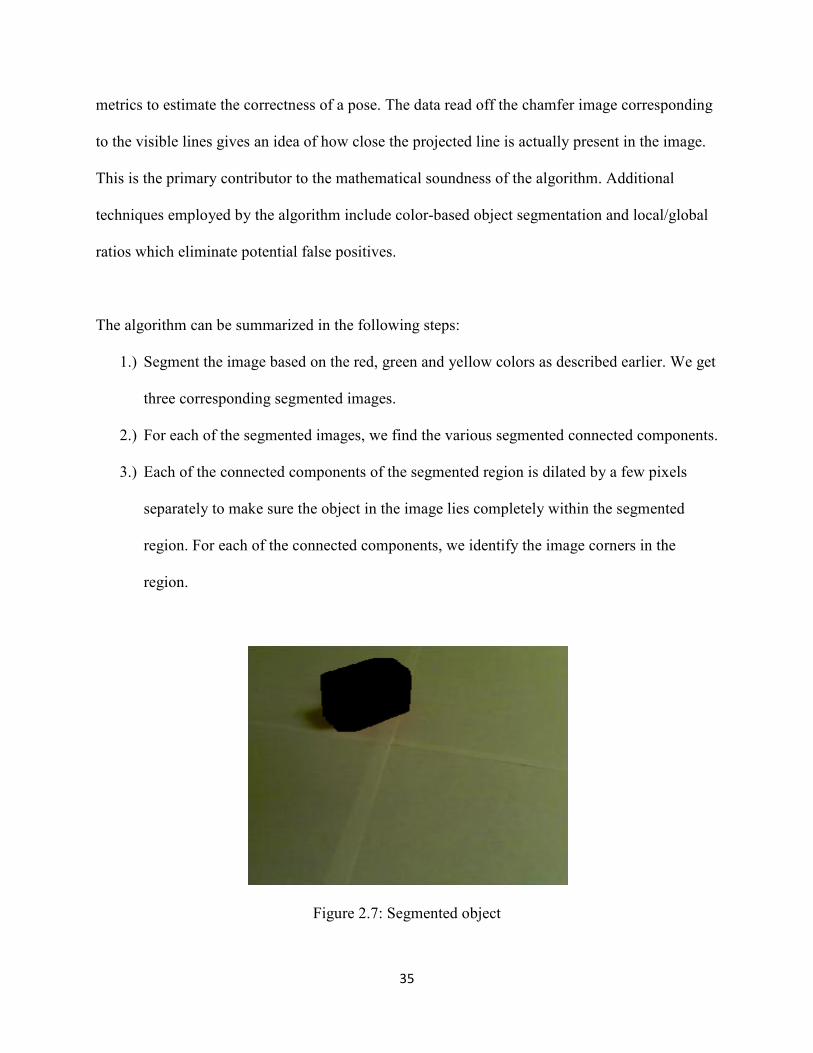
The algorithm can be summarized in the following steps:

1.) Segment the image based on the red, green and yellow colors as described earlier. We get

three corresponding segmented images.

2.) For each of the segmented images, we find the various segmented connected components.

3.) Each of the connected components of the segmented region is dilated by a few pixels

separately to make sure the object in the image lies completely within the segmented

region. For each of the connected components, we identify the image corners in the

region.

Figure 2.7: Segmented object

36

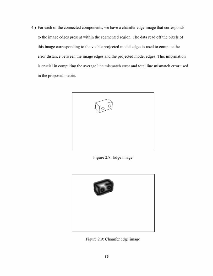
4.) For each of the connected components, we have a chamfer edge image that corresponds

to the image edges present within the segmented region. The data read off the pixels of

this image corresponding to the visible projected model edges is used to compute the

error distance between the image edges and the projected model edges. This information

is crucial in computing the average line mismatch error and total line mismatch error used

in the proposed metric.

Figure 2.8: Edge image

Figure 2.9: Chamfer edge image

37

5.) In our database, we have a set of 3-D object models which are present in the image. We

try and fit each of the models to each of the connected components of the segmented

region of image successively.

6.) To do this, we pick out all permutations of three image corner-point sets and associate

them with the corners of each of the unique triangles that make up the 3-D model.

Figure 2.10: Prominent corners in the segmented region

7.) For each such association, we get a perspective three-point problem with multiple

solutions.

8.) Each of the solutions is translated into the appropriate rotation and translation matrices.

9.) The rotation and translation matrices combined with the camera calibration matrix helps

find the get the positions of the new 3-D coordinates and project them onto the image

plane.

10.) Since the new 3-D model pose is known, the sets of visible edges can be computed.

These edges are now compared against the edge-based chamfer distance image. The

38

visibility of each of the surfaces is calculated by computing the surface normal of each

of the surfaces with ordered vertices after projection onto the image plane. If the surface

normal has a negative Z component, we say that the surface faces the camera and is

hence visible. In this process, care must be taken to make sure that all the projected

vertices lie within the image boundaries. If any of the vertices overshoot these

boundaries, the pose can be directly discarded.

11.) Now we compute the average pixel mismatch error for each of the visible lines. If the

average pixel error for a line is below a predefined threshold, we consider that line a

match.

12.) We also compute the total mismatch error for all the matched lines.

13.) The discrete metric ranks the poses in a lexicographical order, with the poses with

higher line matches and then lower total mismatch error for all the visible given a higher

priority. Thus, the pose with the minimum total line mismatch error among the poses

with the maximum number of line matches is considered the best estimate.

14.) The continuous metric, on the other hand, is formulated as a summation of a function of

average line mismatch error and total mismatch error for each of the lines. This gives us

a single number whose magnitude gives a quantitative representation of the

appropriateness of the pose.

39

Elimination of false positives:

For each of the object 3-D poses projected onto the image plane, we define two ratios and

make sure they are above a predefined threshold:

1.) Global ratio: Ratio of the area of the convex hull of the projected model and the

segmented out region.

2.) Local ratio: Ratio of the area of the intersection of segmented region and the convex hull

and the area of the convex hull itself.

Optionally, we might employ a constraint on the translation vector to make sure the object’s

estimated pose does not go any further beyond a predefined value.

Figure 2.11: Computing Average and Total Line Mismatch Error

Let Ai be the average mismatch error and Ti be the total mismatch error for line i. The

average mismatch error of line i is defined as the average value of the pixels in the chamfer

image that correspond to the ith

visible model line projected onto the image plane. The total

mismatch error of line i is defined as the total value of the pixels in the chamfer image that

correspond to the ith

visible model line projected onto the image plane.

40

The average and total mismatch error for red line 1 shown in Figure 2.11 is lesser than

that of line 2 due to a better match with the darker regions of the chamfer image.

Let the mismatch threshold be Tm. Let the total number of visible lines be N. The

continuous metric Mc is defined by the equation:

1

i

#A

c i

i

M T e=

= −∑

A pose with a higher value of Mc is said to be a better pose estimate.

For evaluating the discrete metric, we consider two parameters:

1.) Count – it refers to the number of visible lines with an average mismatch error lesser than

or equal to Tm.

2.) Total – it refers to the sum of the mismatch error of all the visible lines which have an

average mismatch error lesser than or equal to Tm.

The possible poses are arranged in a lexicographical order with the poses arranged in

order of decreasing “count” values. Among the poses with equal values of “count”, the poses are

rearranged in the order of increasing “total” values. Thus, the poses with the highest value of

= Sum of all corresponding pixel valuesiT

Sum of all corresponding pixel values

Total number of line pixelsiA =

41

“count” are considered to be the better poses. Among them the pose with the least value of

“total” is taken to be the best pose.

Figure 2.12: Global and Local ratios used in the algorithm

In Figure 2.11, the ellipse represents the segmented out region while the rectangle

represents the convex hull of the pose of the 3-D object projected onto the image plane.

The global ratio, GR is defined as:

Area of yellow region + Area of green regionGR

Area of red region + Area of yellow region=

The local ratio, LR is defined as:

Area of yellow regionLR

Area of red region + Area of yellow region=

42

CHAPTER THREE

RESULTS AND DISCUSSION

3.1 DATA USED AND METHODOLOGIES

The experiment can be summarized as follows. A USB web camera was mounted on a

camera stand and was positioned to look down at different assembly scenes. The images of the

assemblies were then stored in a standard format; the jpeg image format was used in this

experiment. A measure of the true pose of the assembly components was done manually - this

will be described later in this section. The images were fed as a parameter to the algorithm

implemented in Matlab to produce the estimated poses of the assembly objects.

The images of the object were taken under typical uneven home illumination conditions

under an overhead CFL light source. The objects used were Screw Blocks with rounded corners

and holes with little or no surface texture information. The camera used was a Logitech C250

webcam which can afford a maximum resolution of 640x480. We use a more typical webcam

resolution of 320x240 in our experiments to put to test the strength of the algorithm. The

webcam was fixed in a camera stand of height of about 20 cm with an angle of descent of about

45 degrees.

About 22 images of the Lego blocks were taken under varying lighting conditions and a

variety of poses. 17 of these images included the red Lego cuboid in the actual image, 13

included the green Lego cube and 17 included stray yellow cube(s) for providing clutter and

43

noise which is precisely the conditions under which the algorithm is designed to work robustly.

The cuboid used was of the dimensions 6x3x3cm while the cube was of the dimensions

3x3x3cm.

The algorithm was implemented in Matlab version R2007 under the Windows Vista

(Service pack 1) operating system. The OpenCV 2.0 implementation for camera calibration was

used to get the camera calibration matrix while the Matlab corner detector implementation by He

and Yung was used to detect the prominent corners in the images.

Implementation details:

Prominent Matlab function routines developed:

1.) CheckBlob.m: This function is the top-level function which calls all the other functions.

This function takes the image file, 3D object model, and threshold parameters for

segmented image dilation, corner detector thresholds and discrete metric threshold.

2.) SegmentCC.m: It is called by CheckBlob.m recursively to return the discrete connected

components of blobs of each color separately by calling the function implemented in

Segment.m file.

3.) Controlpointgen.m: This function generates the set of unique triplets of 3-D model points

(Which we call control point sets) which by themselves are enough to exhaustively

search the entire possible pose mapping from the object model to 2D image points for a

symmetric object like a cube or a cuboid.

44

4.) P3P_solve.m: This function solves the Perspective 3-point pose estimation problem

mentioned earlier and returns the depths of the image points.

5.) RT.m: This function converts the solution to the P3P problem into the corresponding

rotation and translation matrices.

6.) Edge_distance_compare_match.m: It takes the chamfer edge distance image of the edge

image, the projected image points, the set of visible lines for the estimated pose and the

threshold for computing the discrete metric. It returns a measure of pose suitability

computed both using the discrete and the continuous metrics discussed earlier.

7.) Convhullparea.m: This function computes the Local and Global ratios described earlier.

It takes the projected image model points and the segmented image as parameters.

We use two threshold values for generating the corners and the corresponding edges

using the corner detector. The first threshold which is used for obtaining the set of corners is

made moderately high so that only the prominent image corners are chosen. The second

threshold which is used for specifying the percentage of edges detected is made low so that a

sufficiently high amount of edge information is used for pose estimation. This approach

increases the reliability of the pose estimated while maintaining relatively low pose computation

times.

The true pose of the object was estimated by carefully selecting the corresponding image

points for the visible 3-D model points and solving the pose estimation problem with known

correspondences discussed earlier. Further pose refinement was done using a GUI developed for

fine-tuning pose estimates through close visual inspection. This could have been done in an

45

alternate way: by physically measuring the rotation and translation with respect to a world

coordinate system. Physical measurements are not, in practice, completely error free and the

measurements might prove quite unrepeatable in cases where we might need to come back to a

particular exact test setup in the future for additional measurements. Since we would be fine-

tuning these estimates through close visual inspection using the Matlab GUI developed for this

purpose anyway, one might argue that there would be little difference between the two estimates.

The values of the standard tuning parameters used in the algorithm implementation are:

Global ratio: 50 percent

Local Ratio: 50 percent

Extent of dilation of segmented region: 15 pixels

Discrete metric threshold: 2 pixels

Translation constraint: 40 cm from camera focus

Threshold used to detect prominent corners: 0.5

Threshold used to detect prominent edges: 0.1

3.2 RESULTS

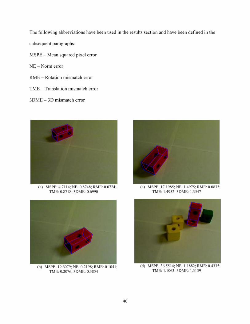
This section presents the typical results got from the program run. The blue lines

represent the measured pose, which is also assumed to be the true pose of the object. The red

lines are obtained by plotting the 3D model on the image plane using the best pose computed

during the program run.

46

The following abbreviations have been used in the results section and have been defined in the

subsequent paragraphs:

MSPE – Mean squared pixel error

NE – Norm error

RME – Rotation mismatch error

TME – Translation mismatch error

3DME – 3D mismatch error

(a) MSPE: 4.7114; NE: 0.8748; RME: 0.0724;

TME: 0.8718; 3DME: 0.6990

(b) MSPE: 19.6079; NE: 0.2198; RME: 0.1041;

TME: 0.2076; 3DME: 0.3854

(c) MSPE: 17.1985; NE: 1.4975; RME: 0.0833;

TME: 1.4952; 3DME: 1.3547

(d) MSPE: 36.5514; NE: 1.1882; RME: 0.4335;

TME: 1.1063; 3DME: 1.3139

47

(e) MSPE: 64.1339; NE: 0.7009; RME: 0.1870;

TME: 0.6768; 3DME: 0.6475

(f) MSPE: 338.306; NE: 1.8328; RME: 0.8299;

TME: 1.7586; 3DME: 2.2175

(g) MSPE: 18.0037; NE: 0.7518; RME: 0.0524;

TME: 0.7500; 3DME: 0.8114

Figure 3.1 (a-g) – True and estimated poses of the red cuboid

(a) MSPE: 0.7773; NE: 0.5490; RME: 0.6323;

TME: 0.0390; 3DME: 0.6323

(b) MSPE: 16.8409; NE: 0.5464; RME: 0.0780;

TME: 0.5408; 3DME: 0.5263

48

(c) MSPE: 74.9824; NE: 2.3954; RME: 1.5019;

TME: 2.3715; 3DME: 2.0771

Figure 3.2 (a-c) – True and estimated poses of the green cuboid

Figure 3.3: 3D Mismatch Error Performance plot

49

Figure 3.4: Translation Mismatch Error Performance plot

3.3 DISCUSSION

The performance plot shown in Figure 3.3 summarizes the accuracy of the algorithm

which was tested on a 22-image dataset with 28 assembly component poses considered. As

observed from the graph, the algorithm works with a 3D mismatch error of less than 2.5cm error

in 90% of the cases (Groups 1 and 2 together) and less than 1cm error in 53% of the cases

(Group 1).

The proposed algorithm works quite well in cases in relatively uniform lighting

conditions where the corner features appear more distinct. In cases where the features are

50

indiscernible owing to poor lighting, occlusions due to surrounding objects or the actual pose of

the object itself with few surfaces visible, the detected pose, as is evident from the images is less

accurate. As evinced by the results, the algorithm works pretty well for well-lit objects much of

which is visible in the image. The algorithm is hampered in a few cases owing to the presence of

heavy shadows by the surrounding objects which affect the estimated orientation of the target

object.

The strength of the algorithm lies in its ability to work despite all these conditions and

give a result that is not off from the true one by a large margin. The segmentation approaches

make sure that the object translation is close enough to the true one. The discrete line-match

based metric tries to make sure that most of the object edges are matched as closely as possible

making the estimate as close as possible to the true one. The continuous metric is found to be

more prone to errors compared to the discrete metric in converging to the true pose of the object.

The reason for this could be attributed to the nature of the continuous metric which is designed to

take the global metrics into consideration much more than the local metrics. This is in sharp

contrast with the discrete metric which gives a higher preference to local matching thresholds.

The discrete metric has been found to give consistently better results compared to the

continuous metric. Thus, we take the pose computed by the discrete metric as the final output of

the implementation and list the match computed by the continuous metric along for reference.

To adapt this algorithm for a disassembly process, a good approach would be to find out

the subassemblies with the best metric and try removing them from the assembly first as their

51

pose is more reliable. This process is repeated until there are no more subassemblies left in the

scene.

The results presented in the previous section illustrate the typical outputs generated by

the algorithm implementation. The mean squared pixel error is defined as the average of the

squared distances between the corresponding projected image model points and the image points.

The norm error refers to the minimum norm of the difference of the measured object pose and

the estimated poses (with all the possible poses generated by equivalent local rotations

considered).

The norm error gives a better picture of the actual difference in poses as it works for an

N-dimensional space (In our case, N=3). On the other hand, Mean square pixel error is highly

sensitive to slight changes in local orientation of the object and comparatively static to

translation, especially along the Z-axis.

The drawback with the norm error is that it does not distinguish between the rotation and

translation mismatches. To present a clearer picture, we compute and present these mismatch

values separately. The translation mismatch is defined as the norm of the difference between the

vectors TM and TC. The rotation mismatch, on the other hand, is defined as the norm of the

matrix 1[ . ]I RM RC −− , or equivalently, norm of the matrix 1[ . ]I RC RM −− . Here, RM and TM

are the rotation and translation matrices obtained from the actual measurement and are assumed

to represent the true pose of the object. RC and TC are the rotation and translation matrices

computed during the program run and represent the estimated object pose. Since the norm error

52

involves computing the norm of the matrix containing difference of both the rotation and

translation vectors, it is hard to intuitively understand the physical significance of its

mathematical value.

The most natural choice of error measurement metric would be the 3D mismatch error

metric. This metric is defined as the average 3D distance error between the corresponding

corners of the true and the estimated object poses. This metric, unlike the others, is quite intuitive

as it gives us a way to visualize the mismatch errors between the poses in 3D space. It is for this

reason that this error metric is preferred over the others for the Mismatch error-Population plot.

The performance plot gives the relation between the percentages of population with the

corresponding 3D error metric below a given value. As mentioned before, in ninety percent of

the cases, the 3D error was less than 2.5cm on an average; and in fifty three percent of the cases,

the 3D error was less than 1cm. Close observation of the plot gives rise to the hypothesis of the

existence of three discrete groups of object images, each having a distinct range of error. Further

investigation reveals that group 1, with the lowest error; consists primarily of the cases where the

object remains relatively unaffected by occlusions or shadows. Group 2, on the other hand, is

moderately affected by both occlusions and shadows, while in cases in group 3, are severely

occluded and subject to heavy shadows. This suggests a clear metric-based demarcation between

the various cases considered.

The adopted exhaustive search technique, on a higher level looks computationally

expensive making its implementation appear infeasible for any practical application. This is

53

particularly true in our case where we iterate through each of the connected components of each

color segmented out and subsequently try matching every model in the database to the target

region. On closer observation, we realize this problem has a huge search space that can easily be

reduced to a much smaller one. This is evident from the practical implementation of the

algorithm, where the search is done in typically less than 3 minutes for the given images. Thus,

the drawback of having a high computation order and time is partly offset by filtering out the

majority of possible poses which turn out to be false positives for the most part using specific

techniques incorporated in the algorithm which have been discussed earlier.

The algorithm primarily derives its reasonably reliable performance from the fact that

reliable, repeatable color-based segmentation can be performed on objects with most of the false

positives can be done away with using the Global and Local ratios discussed earlier. We further

reduce the computational time by using specific triplets of 3-D model points which are chosen in

such a way that at least one valid mapping between a triplet and an identified set of three valid

object image corner features exist. In other words, this set of triplets is sufficient to generate all

the possible valid poses while simultaneously eliminating any pose redundancies along the way.

In addition to this, feeding two appropriate thresholds to the corner detector, one kept low to just

get a set of corner points that have at least three valid object corners for pose estimation, and

another kept high to get a sufficient number of edges to enhance reliability of the estimated pose.

Since we iterate through the corners alone, the computation time is considerably reduced. While

these approaches do not change the order of computation as such, but the overall number of

iterations that one has to take to come up with a reasonable pose estimate is considerably

reduced.

54

The algorithm, in its current state, places a greater focus on arriving at a more reliable

solution rather than an optimal, computationally less expensive solution and consequentially

takes a disproportionate amount of time for utility in a fast-paced, real time scenario. We will

proceed to discuss how this handicap could be potentially eliminated in the next chapter.

55

CHAPTER FOUR

CONCLUSIONS AND FUTURE WORK

The results obtained indicate that the algorithm is reasonably suited for toy problems

involving disassembly of small assemblies with few features. The experiments performed were

in a largely structured environment under relatively uneven illumination conditions and moderate

occlusions. However, the proposed algorithm can be expected to work in most cases even in an

unstructured environment, provided reliable segmentation is achieved.

A major source of error in results produced by the algorithm arises from the modules

used to detect the corners and edges. The 3D object is modeled as a set of edges forming faces

with sharp corners. The actual object model, on the other hand, possesses rounded corners which

are often not detected by the corner detector used. The algorithm remains relatively resistant to

this weakness since it requires just three true object corners be detected in the image with

negligible error. Much of this drawback with corner detection could be overcome if we

employed an alternate approach where edge detection is based on regions with similar local

color/texture rather than on local gradients. Once we have a reliable method to detect edges, the

problem of obtaining reliable corners will be a natural consequence. This approach would enable

us to have a reliable pose estimate even when similar-looking objects are stacked together in the

image. However, this implies we cannot employ this technique on a largely texture-free object.

Since most real-world assemblies can be assumed to have surface-texture in some form, this idea

might be useful to consider.

56

Another notable weakness with the algorithm implementation stems from the color-based

segmentation technique. While the color-based segmentation technique is extremely reliable for

uniformly colored objects, problems arise when similar colored objects are placed very closely

and their dilated segmented regions in the image overlap. This calls for an intelligent, content-

aware segmentation technique.

The algorithm has been found to produce a higher pose-estimate error in cases where

heavy shadows are predominant, leading to false edges. As discussed earlier, while one might

argue that this problem could be eliminated using color/texture-based edge detection to arrive at

a set of true edges, we also could view this problem a little differently. High pose estimate errors

arise when the number of line matches is high owing to multiple object model line matches on

the same image line. To offset this, we could potentially introduce a constraint where 3D object

model edges which map a little too close on the image plane be appropriately penalized. Again,

the drawback with this approach is that such cases are quite possible in real images and errors

may arise in certain cases due to the penalization itself.

The algorithm, at present, works well for objects with corners (both sharp and rounded)

and well defined sides. However, the algorithm is not expected to work on a surface devoid any

noticeable corners and straight edges. This could be viewed as a drawback in for an algorithm

like this as and can be largely expected to fail while attempting to find a solution for the pose of

a smooth object like a sphere or an ellipsoid in an image given an approximate 3-D model

constructed using a Delaunay triangulation. Approximating a rounded object usually entails

having a large number of object model vertices. Thus, even if at least three false corners are

57

detected on the smooth object, they could still be used to determine the object pose. An

implementation that requires permutations of all the possible corner points in the model would be

highly impractical and would lead to very high implementation runtime. It is imperative that an

alternate formal approach to deal with such cases be formulated to obtain an algorithm that

works on a bigger class of objects.

An alternate approach would be to have an automated technique to map features on 3D

objects onto an image plane and find out the appropriate correspondences between the synthetic

and the real images. This is closely related to the method discussed in literature survey section

where a given database is searched for the best matching pose. Unfortunately, such an approach

would not be feasible for objects with little or no identifiable visual surface features - much like

the ones we have tested our algorithm on. Also, we now have an additional correspondence-

determination problem at hand.

To overcome the problem of pose estimation of occluded objects, one could first find out

the poses of objects with the highest metric in 3-D space. The poses of objects with a lower

metric could subsequently be corrected based on the poses we place a greater trust on (The poses

with a higher metric).

Looking at the problem of occlusion with the disassembly process in perspective, we can

expect this to pose an insignificant practical impediment to the real problem we are trying to

solve. This is because we can build a system that would actuate the removal of objects in the

58

order of their decreasing metric. This would subsequently ensure the visibility of the once-

occluded objects leading to the dismantling of the entire assembly over time.

A second look at the algorithm would reveal that the search process is really independent

of the previous state that was evaluated. This implies that the whole algorithm could be

parallelized and made to run in real-time using a cluster of GPU-enhanced machines. This

arrangement would be another step in building a machine to emulate the human brain in figuring

out the best way in taking apart a given assembly without much delay.

Concurrently, one could adopt a line-based version of an iterative algorithm like the

SoftPOSIT. Starting out with initial random pose guesses from every local region of the camera

view volume and letting them converge independently would result in a population of potentially

viable poses. Each of these poses could then be subject to evaluation using the techniques

discussed in this thesis.

59

CHAPTER FIVE

REFERENCES

[1] T. Yuksel and I. Baylakoglu, "Recycling of Electrical and Electronic Equipment,

Benchmarking of Disassembly Methods and Cost Analysis," in Electronics & the

Environment, Proceedings of the 2007 IEEE International Symposium on, 2007, pp. 222-

226.

[2] A.C. Sanderson, "Assemblability based on maximum likelihood configuration of

tolerances," Robotics and Automation, IEEE Transactions on, vol. 15, no. 3, pp. 568-572

1999.

[3] L.S. Homem de Mello and A.C. Sanderson, "AND/OR graph representation of assembly

plans," Robotics and Automation, IEEE Transactions on, vol. 6, no. 2, pp. 188-199 1990.

[4] K.W. Khawaja, D. Tretter, A.A. Maciejewski and C.A. Bouman, "Automated assembly

inspection using a multiscale algorithm trained," in Robotics and Automation, 1994.

Proceedings., 1994 IEEE International Conference on, 1994, pp. 3530-3536 vol.4.

[5] C. Bauckhage, S. Kronenberg, F. Kummert and G. Sagerer, "Grammars and discourse

theory to describe and recognize mechanical assemblies," in Joint IAPR International

Workshops SSPR 2000 and SPR 2000, 2000, pp. 173-82.

60

[6] C. Bauckhage, F. Kummert and G. Sagerer, "A structural framework for assembly modeling

and recognition," Computer Analysis of Images and Patterns, Proceedings, vol. 2756, pp.

49-56 2003.

[7] Hongbo Shan, Shuxia Li, Jing Huang, Zhimin Gao and Wei Li, "Ant Colony Optimization

Algorithm-Based Disassembly Sequence Planning," in Mechatronics and Automation, 2007.

ICMA 2007. International Conference on, 2007, pp. 867-872.

[8] D.F. Dementhon and L.S. Davis, "Model-based object pose in 25 lines of code,"

International Journal of Computer Vision, vol. 15, no. 1-2, pp. 123-41, 06 1995.

[9] P. David, D. DeMenthon, R. Duraiswami and H. Samet, "Simultaneous pose and

correspondence determination using line features," in Computer Vision and Pattern

Recognition, 2003. Proceedings. 2003 IEEE Computer Society Conference on, 2003, pp. II-

424-II-431 vol.2.

[10] P. David and D. DeMenthon, "Object recognition in high clutter images using line

features," in Computer Vision, 2005. ICCV 2005. Tenth IEEE International Conference on,

2005, pp. 1581-1588 Vol. 2.

[11] H.F. Ugurdag, S. Goren and F. Canbay, "Correspondenceless Pose Estimation from a single

2D image using classical mechanics," in Computer and Information Sciences, 2008. ISCIS

'08. 23rd International Symposium on, 2008, pp. 1-6.

61

[12] M.A. Fischler and R.C. Bolles, "Random sample consensus: A paradigm for model fitting

with applications to image analysis and automated cartography," Commun ACM, vol. 24, no.

6, pp. 381-95, 06 1981.

[13] F. Toyama, K. Shoji and J. Miyamichi, "Model-based pose estimation using genetic

algorithm," in Pattern Recognition, 1998. Proceedings. Fourteenth International

Conference on, 1998, pp. 198-201 vol.1.

[14] M. Kayanuma and M. Hagiwara, "A new method to detect object and estimate the position

and the orientation from an image using a 3-D model having feature points," in Systems,

Man, and Cybernetics, 1999. IEEE SMC '99 Conference Proceedings. 1999 IEEE

International Conference on, 1999, pp. 931-936 vol.4.

[15] C. Rossi, M. Abderrahim and J.C. Diaz, "EvoPose: a model-based pose estimation

algorithm with correspondences determination," in Mechatronics and Automation, 2005

IEEE International Conference, 2005, pp. 1551-1556 Vol. 3.

[16] D. Rother and G. Sapiro, "Seeing 3D objects in a single 2D image," in Computer Vision,

2009 IEEE 12th International Conference on, 2009, pp. 1819-1826.

[17] D.G. Lowe, "Object recognition from local scale-invariant features," in Computer Vision,

1999. The Proceedings of the Seventh IEEE International Conference on, 1999, pp. 1150-

1157 vol.2.

62

[18] S. Savarese and Li Fei-Fei, "3D generic object categorization, localization and pose

estimation," in Computer Vision, 2007. ICCV 2007. IEEE 11th International Conference on,

2007, pp. 1-8.

[19] R.M. Haralick and Joo Hyonam, "2D-3D pose estimation," in Pattern Recognition, 1988.,

9th International Conference on, 1988, pp. 385-391 vol.1.

[20] Zhengyou Zhang, "Flexible camera calibration by viewing a plane from unknown

orientations," in Computer Vision, 1999. The Proceedings of the Seventh IEEE International

Conference on, 1999, pp. 666-673 vol.1.

[21] C.H. Xiao and N.H.C. Yung, "Corner detector based on global and local curvature

properties," Optical Engineering, vol. 47, no. 5, pp. 057008-1, 05 2008.

[22] C.S. Langley and G.M.T. D'Eleuterio, "Neural network-based pose estimation for

fixtureless assembly," in Computational Intelligence in Robotics and Automation, 2001.

Proceedings 2001 IEEE International Symposium on, 2001, pp. 248-253.