Colby CollegeDigital Commons @ Colby

Honors Theses Student Research

2006

Position tracking and motion prediction usingFuzzy LogicPatrick RodjitoColby College

Follow this and additional works at: http://digitalcommons.colby.edu/honorsthesesColby College theses are protected by copyright. They may be viewed or downloaded from this sitefor the purposes of research and scholarship. Reproduction or distribution for commercial purposesis prohibited without written permission of the author.

This Honors Thesis is brought to you for free and open access by the Student Research at Digital Commons @ Colby. It has been accepted for inclusionin Honors Theses by an authorized administrator of Digital Commons @ Colby. For more information, please contact mfkelly@colby.edu.

Recommended CitationRodjito, Patrick, "Position tracking and motion prediction using Fuzzy Logic" (2006). Honors Theses.Paper 520.http://digitalcommons.colby.edu/honorstheses/520

Position Tracking and Motion Prediction Using Fuzzy Logic

Patrick Rodjito

Honors Thesis Department of Computer Science

Advisors:

Randolph M. Jones, Department of Computer Science Joseph E. Atkins, Department of Psychology

Colby College Spring 2006

II

Acknowledgments This project would not have happened if not for Prof. Joseph E. Atkins, who came up with the idea a year prior to the start of the project. Since then, Joe spent countless hours working closely with us on the project. The success of the position tracking methodology that is currently in place is a direct result of Joe’s contribution to the project. It would not have been possible if not for Prof. Randolph M. Jones who approved of the project and undertook the role of project manager and mentor. Randy contributed greatly to the writing produced from our yearlong research. We are also grateful to Prof. Dale J. Skrien, our thesis reader, and Prof. Clare Bates Congdon who aided us in the final editing process. Many thanks to the five Science students, Nico Mwai, Tomas Vorobjov, Mao Zheng, Andreea V. Olea, and Timothy D. Monahan who participated in the experiments, and to Michael E. Dieffenbach, who provided his expertise in designing and conducting our psychology experiments.

III

IV

Table of Contents Preface-------------------------------------------------------------------------------VII Chapter 1: Introduction--------------------------------------------------------------1 1.1 Brief History of Fuzzy Logic----------------------------------------------------------------1 1.2 Introduction to Fuzzy Inference Systems--------------------------------------------------2 1.3 Project Goals-----------------------------------------------------------------------------------4 Chapter 2: Case Studies-------------------------------------------------------------5 2.1 Related Work on Fuzzy Logic--------------------------------------------------------------5 2.1.1 Case Study I: Small Engine Control -----------------------------------------------------------6 2.1.2 Case Study II: Robot Head Visual Tracking---------------------------------------------------10 2.1.3 Case Study III: Motion Tracking and Prediction----------------------------------------------14 2.1.4 Case Study IV: Urban Canyon Vehicle Navigation-------------------------------------------18 2.2 Comparison of Case Studies---------------------------------------------------------------- 23 Chapter 3: Hardware and Software-----------------------------------------------25 3.1 Worktable-------------------------------------------------------------------------------------25 3.2 Computer--------------------------------------------------------------------------------------25 3.3 Camera---------------------------------------------------------------------------------------- 25 3.4 Matlab----------------------------------------------------------------------------------------- 26 Chapter 4: Image Acquisition and Processing-----------------------------------27 4.1 Object Pattern---------------------------------------------------------------------------------27 4.2 Image Acquisition and Pre-Processing----------------------------------------------------27 4.3 Object Hunting with Linear Filtering------------------------------------------------------28 4.4 Weeding out Aliases-------------------------------------------------------------------------29 4.5 Stat Array--------------------------------------------------------------------------------------30 Chapter 5: Position Tracking Fuzzy Logic System-----------------------------33 5.1 Expert Knowledge---------------------------------------------------------------------------33 5.1.1 Analysis of Object Energies-------------------------------------------------------------------- 33 5.1.2 Measuring Human Performance----------------------------------------------------------------35 5.2 Direction Inference System-----------------------------------------------------------------35 5.2.1 Fuzzification---------------------------------------------------------------------------------------36 5.2.2 Rule Base-------------------------------------------------------------------------------------------37 5.2.3 Defuzzification-------------------------------------------------------------------------------------39 5.3 Object Rotation------------------------------------------------------------------------------- 40 5.4 ID Fuzzy Inference System------------------------------------------------------------------40 5.4.1 Fuzzification----------------------------------------------------------------------------------------41 5.4.2 Rule Base--------------------------------------------------------------------------------------------42 5.4.3 Defuzzification-------------------------------------------------------------------------------------42 5.5 Evaluations and Conclusions----------------------------------------------------------------43

V

Chapter 6: Tuning-------------------------------------------------------------------47 6.1 Direction FIS Version History (Version 1 through 4.1)---------------------------------47 6.2 ANFIS------------------------------------------------------------------------------------------53 Chapter 7: Project Conclusions and Future Work------------------------------55 7.1 Conclusion-------------------------------------------------------------------------------------55 7.2 Future Work-----------------------------------------------------------------------------------56 Bibliography-------------------------------------------------------------------------57 Appendix: Code Listings-----------------------------------------------------------59

VI

Preface Humans find it difficult sometimes to make out objects that are captured using a low- resolution camera. This is probably because the images are fuzzy. Nevertheless, the human brain will try to make up for the incomplete or imprecise information by guessing or generalizing. Using a computer to analyze data that is imperfect and noisy is probably a computationally expensive process, if it’s done by conventional means. However, an inference system that mimics the way human handles incomplete information may be able to arrive at reasonably good answers using fewer computations. Such a system is faster than its conventional counterpart, as it does not require as many data points to arrive at an answer, and cheaper to build, as its supporting equipments (in this case the camera) can have lower precisions. Fuzzy logic (FL) is a highly debated topic among mathematicians. Some mathematicians think that FL does not really qualify as something new and is actually no different than probability theory, while others belief that it brings nothing to the table that standard binary logic has not. However, many fought for the notion that FL and standard logic complement each other, and only upon both can all scientific thought, probabilistic or precise be built. FL is the implementation of one’s logic and understanding of this imprecise, subjective, human world and made very real the possibility of an AI whose ability to adapt can rival ours. It is no wonder that many industrialists and scientists embraced FL as a solution to complex problems despite the denouncement of their peers. FL is already used in some home appliances and subway systems and it’s just a matter of time for FL to become ubiquitous. Unlike with traditional, computationally expensive algorithms, with FL one does not have to own a fast computer or very precise measuring instruments to get good results. At lower costs, FL provides a simple way to arrive at a definite conclusion based upon vague, ambiguous, imprecise, noisy, or missing input information. This is a facet of AI that appears to resemble human intuition in an important way: the ability to make quick and urgent judgment calls, on the spot, without the need to be absolutely certain of the input. The benefit brought by a low-cost solution like FL to mankind is widespread, as not only researchers of high caliber but also everyone can benefit from it. In the pages to come, we will delve, as deeply as the diagrams and expositions will allow, into the implementation of a fuzzy system designed for the purpose of tracking and predicting the motion of light-colored objects on dark background. Before that, however, is a brief history and introduction to FL.

VII

Chapter 1: Introduction 1.1 Brief History of Fuzzy Logic As Plato once indicated, there was a third region beyond true and false where opposites are "tumbled about." In the 20 centuryth , Jan Lukasiewicz proposed a three-valued logic (true, possible, false). [3]

In 1965, a renowned mathematician, Lofti A. Zadeh, of University of California at Berkeley proposed Fuzzy Logic (FL) in a paper detailing the mathematics of fuzzy sets theory [1,10]. Zadeh further elaborated on his ideas in a 1973 paper that introduced the concept of fuzzy variables that belong to a fuzzy set. An industrial application of fuzzy systems soon followed—a cement kiln in Denmark, which came online in 1975 [1]. Although FL was had its origin in America, American and European scientists regarded the theory as non-mathematical and childlike, and it never gained wide acceptance. [14]

Lofti Asker Zadeh Source: [14] In Japan, interest in fuzzy logic was sparked by Seiji Yasunobu and Soji Miyamoto of Hitachi, who, in the year 1985, demonstrated the supremacy of fuzzy control systems in managing acceleration, braking, and stopping of trains in Sendai railway. Two years later, during an international meeting in Tokyo, Takeshi Yamakawa carried out an inverted pendulum* experiment using a set of simple FL chip, where he mounted a wineglass containing a mouse on top of the pendulum. As a direct result of the demonstration, FL became popular in Japan for various industrial and consumer applications. In 1988, 48 Japanese companies established the Laboratory for International Fuzzy Engineering (LIFE). Today, Japanese products that use fuzzy logic range from washing machines to auto focus cameras and industrial air conditioners. [1]

* The “inverted pendulum” experiment is a classic control problem in which a vehicle, or a cart, moves back and forth to try and keep a pole mounted on top of it upright, and widely used as a benchmark for control algorithms such as neural networks and genetic algorithm [14]

1

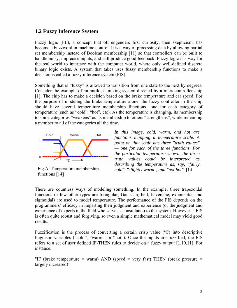
1.2 Fuzzy Inference System Fuzzy logic (FL), a concept that oft engenders first curiosity, then skepticism, has become a buzzword in machine control. It is a way of processing data by allowing partial set membership instead of Boolean membership [11] so that controllers can be built to handle noisy, imprecise inputs, and still produce good feedback. Fuzzy logic is a way for the real world to interface with the computer world, where only well-defined discrete binary logic exists. A system that takes uses fuzzy membership functions to make a decision is called a fuzzy inference system (FIS). Something that is “fuzzy” is allowed to transition from one state to the next by degrees. Consider the example of an antilock braking system directed by a microcontroller chip [1]. The chip has to make a decision based on the brake temperature and car speed. For the purpose of modeling the brake temperature alone, the fuzzy controller in the chip should have several temperature membership functions—one for each category of temperature (such as “cold”, “hot”, etc). As the temperature is changing, its membership to some categories “weakens” as its membership to others “strengthens”, while remaining a member to all of the categories all the time.

In this image, cold, warm, and hot are functions mapping a temperature scale. A point on that scale has three "truth values" — one for each of the three functions. For the particular temperature shown, the three truth values could be interpreted as describing the temperature as, say, "fairly cold", "slightly warm", and "not hot". [14]

Fig A. Temperature membership functions [14]

There are countless ways of modeling something. In the example, three trapezoidal functions (a few other types are triangular, Gaussian, bell, haversine, exponential and sigmoidal) are used to model temperature. The performance of the FIS depends on the programmers’ efficacy in imparting their judgment and experience (or the judgment and experience of experts in the field who serve as consultants) to the system. However, a FIS is often quite robust and forgiving, so even a simple mathematical model may yield good results. Fuzzification is the process of converting a certain crisp value (ºC) into descriptive linguistic variables (“cold”, “warm”, or “hot”). Once the inputs are fuzzified, the FIS refers to a set of user defined IF-THEN rules to decide on a fuzzy output [1,10,11]. For instance: "IF (brake temperature = warm) AND (speed = very fast) THEN (break pressure = largely increased)”

2

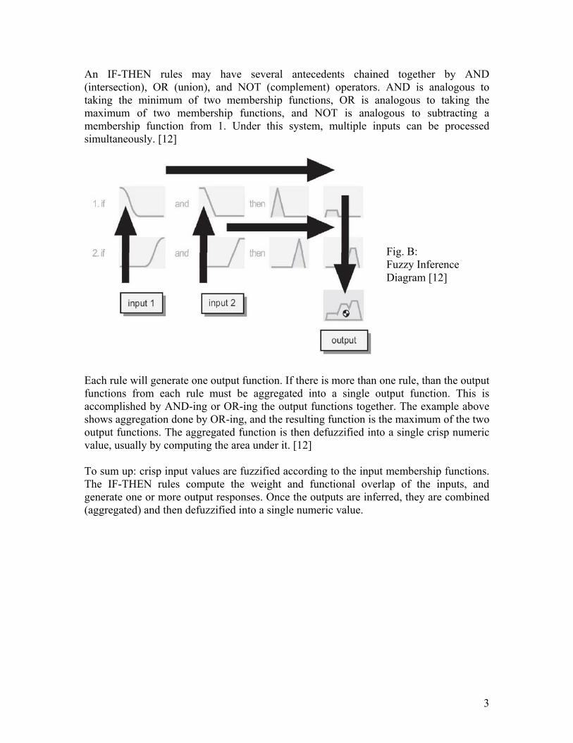
An IF-THEN rules may have several antecedents chained together by AND (intersection), OR (union), and NOT (complement) operators. AND is analogous to taking the minimum of two membership functions, OR is analogous to taking the maximum of two membership functions, and NOT is analogous to subtracting a membership function from 1. Under this system, multiple inputs can be processed simultaneously. [12]

Fig. B: Fuzzy Inference Diagram [12]

Each rule will generate one output function. If there is more than one rule, than the output functions from each rule must be aggregated into a single output function. This is accomplished by AND-ing or OR-ing the output functions together. The example above shows aggregation done by OR-ing, and the resulting function is the maximum of the two output functions. The aggregated function is then defuzzified into a single crisp numeric value, usually by computing the area under it. [12] To sum up: crisp input values are fuzzified according to the input membership functions. The IF-THEN rules compute the weight and functional overlap of the inputs, and generate one or more output responses. Once the outputs are inferred, they are combined (aggregated) and then defuzzified into a single numeric value.

3

1.3 Project Goals With the increasing need for flexibility and adaptivity in computerized systems, the application of fuzzy expert systems is becoming increasingly commonplace in today’s industry [1]. Fuzzy logic expert systems often improve performance by allowing knowledge to generalize without requiring the knowledge engineer to anticipate all possible situations. Thus, for many types of applications, “soft computing” such as Fuzzy logic can incur lower overhead in terms of representing and engineering task knowledge [6]. Our project investigates the application of a fuzzy expert system to position tracking. Previous research showed that Fuzzy Logic could be used to track the motion of a brightly colored object against a dark background, with relatively low development and run-time costs. The system we are developing identifies and tracks multiple objects using unique identification patterns against a dark background. This paper describes the Fuzzy Inference Systems (FIS) for tracking such objects. An essential step to obtaining the fuzzy inputs for the position tracking FIS is to use correlation [13] to obtain the centers of mass of the objects in the image captured using a web camera. Correlation also provides good fuzzy inputs for recognizing object patterns and determining orientation. We investigated various FIS for position tracking in order to identify their strengths and weaknesses. To perform this work, we are using the Matlab fuzzy logic toolkit, which is a simple and flexible tool for designing FIS.

4

Chapter 2: Case Studies 2.1 Related Work on Fuzzy Logic In this chapter, we will take a look at four case studies of control systems using fuzzy logic. These case studies aim to compare various fuzzy inference systems (FIS) by showcasing the fuzzification method, the rule base, and the defuzzification method of each of them. At the end of every case study, we present an analysis of the paper, which usually consists of conjectures about why certain methods are used. The primary purpose of the case studies is to study the techniques that can be used in designing a position tracking FIS.

The second most important goal of the case studies is to give the reader some idea of the contributions that have been made in the relatively young field of fuzzy logic, and some of the great many industrial applications thus far. Although only four of the fuzzy scientific papers we studied are presented, all of them are unique except for the fact that fuzzy logic is central to them all. Unfortunately, certain parts of the case studies are very technical at times. Parts that do not pertain to fuzzy logic are summarized as much as possible so that the reader may focus on just the essential fuzzy logic components. In our Comparison of Case Studies, we will compare the fuzzification, rule base and defuzzification of each case study, and discuss the methodologies that can be adapted for our purposes.

5

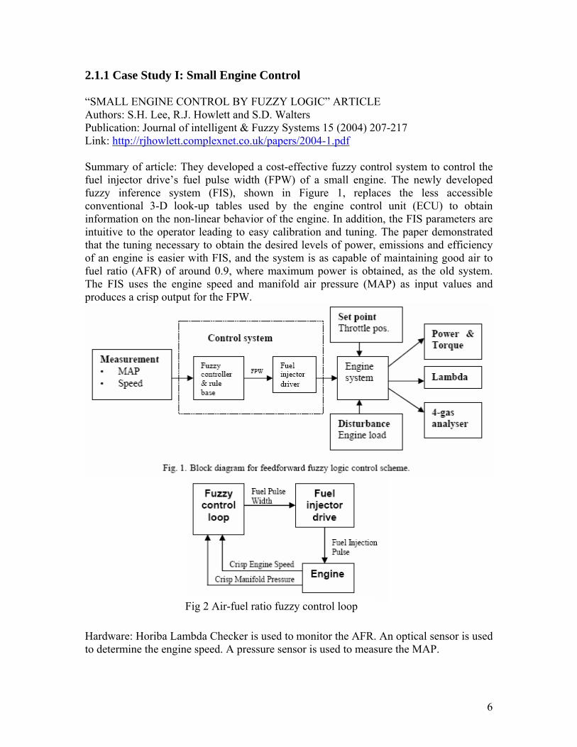
2.1.1 Case Study I: Small Engine Control “SMALL ENGINE CONTROL BY FUZZY LOGIC” ARTICLE Authors: S.H. Lee, R.J. Howlett and S.D. Walters Publication: Journal of intelligent & Fuzzy Systems 15 (2004) 207-217 Link: http://rjhowlett.complexnet.co.uk/papers/2004-1.pdf Summary of article: They developed a cost-effective fuzzy control system to control the fuel injector drive’s fuel pulse width (FPW) of a small engine. The newly developed fuzzy inference system (FIS), shown in Figure 1, replaces the less accessible conventional 3-D look-up tables used by the engine control unit (ECU) to obtain information on the non-linear behavior of the engine. In addition, the FIS parameters are intuitive to the operator leading to easy calibration and tuning. The paper demonstrated that the tuning necessary to obtain the desired levels of power, emissions and efficiency of an engine is easier with FIS, and the system is as capable of maintaining good air to fuel ratio (AFR) of around 0.9, where maximum power is obtained, as the old system. The FIS uses the engine speed and manifold air pressure (MAP) as input values and produces a crisp output for the FPW.

Fig 2 Air-fuel ratio fuzzy control loop Hardware: Horiba Lambda Checker is used to monitor the AFR. An optical sensor is used to determine the engine speed. A pressure sensor is used to measure the MAP.

6

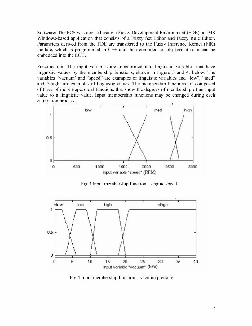
Software: The FCS was devised using a Fuzzy Development Environment (FDE), an MS Windows-based application that consists of a Fuzzy Set Editor and Fuzzy Rule Editor. Parameters derived from the FDE are transferred to the Fuzzy Inference Kernel (FIK) module, which is programmed in C++ and then compiled to .obj format so it can be embedded into the ECU. Fuzzification: The input variables are transformed into linguistic variables that have linguistic values by the membership functions, shown in Figure 3 and 4, below. The variables “vacuum’ and “speed” are examples of linguistic variables and “low”, “med” and “vhigh” are examples of linguistic values. The membership functions are composed of three of more trapezoidal functions that show the degrees of membership of an input value to a linguistic value. Input membership functions may be changed during each calibration process.

Fig 3 Input membership function – engine speed

Fig 4 Input membership function – vacuum pressure

7

Rule Base: The rule base in table 1 shown below has undergone experimental refinement and optimization. Still, the rule base may get changed during future calibration.

Defuzzification: A singleton output membership function is used when the range of valid output values is not continuous. Although the functions are straight lines, there are more than four possible outputs. The combination of different degrees of membership can produce an output other than 142, 143, 143.3, 143.4 and 144.

Table 1: Fuzzy Rule Base

Fig 5 Output membership function – FPW (ms)

Analysis of article: The membership functions for fuzzification of input values are trapezoidal in shape. Perhaps popularity of the trapezoidal shape is second only to the triangular ones. The latter is often employed because it ensures that only one value will attain the highest degree of affinity to a set. With the triangular functions, on the other hand, a set may have multiple values with a degree of membership of 1. Note: degrees of affinity to a membership function are rated from 0 to 1. Consider a FIS tasked with determining the orientation of an object based on the density of the object’s patterns using a ranking system and three membership functions called “high rank”, “mid rank”, and “low rank”. One can argue that since the highest rank is clearly 1, there should only one be value with a degree of membership of 1 to “high rank”, namely rank 1. Therefore using a triangular shape function is most appropriate in this case. After all, it’s a very commonly used shape by FIS designers. It is understandable that one should come to such a conclusion, but there is merit in selecting

8

the trapezoidal shape as well. The strength of fuzzy logic comes from its capacity for error tolerance, and triangular functions are not necessarily the most forgiving. The lens of our web cam is not wide enough to prevent distortion at the sides and more seriously, at the corners. A good error tolerance will help prevent the system from getting confused. For the defuzzification of directions, a trapezoidal or Bell-shaped or any membership function that plateaus will not be appropriate, as say the direction “NE”, has a corresponding value of precisely 45 degree and should be the only value with a degree of affinity of 1. An acute triangular shaped function will better reflect this membership instead of the more accepting trapezoidal shape. Perhaps a Gaussian curve is even more accurate since the climb to the top is not linear. Back to the case study at hand, the defuzzification used in this paper is of Sugeno type, normally used for linear systems or for system with constant outputs [12]. The author must believe that only a handful of values are valid as fuel pulse width: 142 ms, 143.25 ms, 143.4 ms, and 143.44 ms, and which one gets selected to drive the fuel injector depends on the description of the output: “vsmall”, “small”, “med”, “large” or “vlarge” respectively.

9

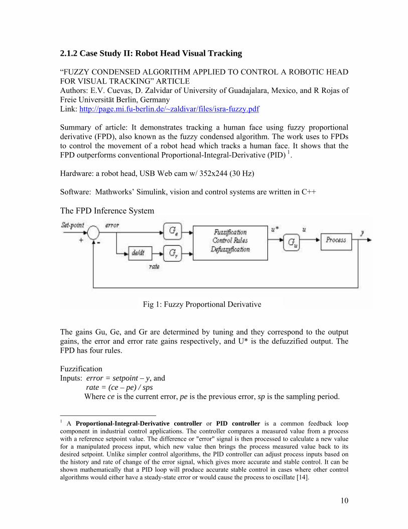
2.1.2 Case Study II: Robot Head Visual Tracking “FUZZY CONDENSED ALGORITHM APPLIED TO CONTROL A ROBOTIC HEAD FOR VISUAL TRACKING” ARTICLE Authors: E.V. Cuevas, D. Zalvidar of University of Guadajalara, Mexico, and R Rojas of Freie Universität Berlin, Germany Link: http://page.mi.fu-berlin.de/~zaldivar/files/isra-fuzzy.pdf Summary of article: It demonstrates tracking a human face using fuzzy proportional derivative (FPD), also known as the fuzzy condensed algorithm. The work uses to FPDs to control the movement of a robot head which tracks a human face. It shows that the FPD outperforms conventional Proportional-Integral-Derivative (PID) 1. Hardware: a robot head, USB Web cam w/ 352x244 (30 Hz) Software: Mathworks’ Simulink, vision and control systems are written in C++ The FPD Inference System

Fig 1: Fuzzy Proportional Derivative The gains Gu, Ge, and Gr are determined by tuning and they correspond to the output gains, the error and error rate gains respectively, and U* is the defuzzified output. The FPD has four rules. Fuzzification Inputs: error = setpoint – y, and rate = (ce – pe) / sps Where ce is the current error, pe is the previous error, sp is the sampling period.

1 A Proportional-Integral-Derivative controller or PID controller is a common feedback loop component in industrial control applications. The controller compares a measured value from a process with a reference setpoint value. The difference or "error" signal is then processed to calculate a new value for a manipulated process input, which new value then brings the process measured value back to its desired setpoint. Unlike simpler control algorithms, the PID controller can adjust process inputs based on the history and rate of change of the error signal, which gives more accurate and stable control. It can be shown mathematically that a PID loop will produce accurate stable control in cases where other control algorithms would either have a steady-state error or would cause the process to oscillate [14].

10

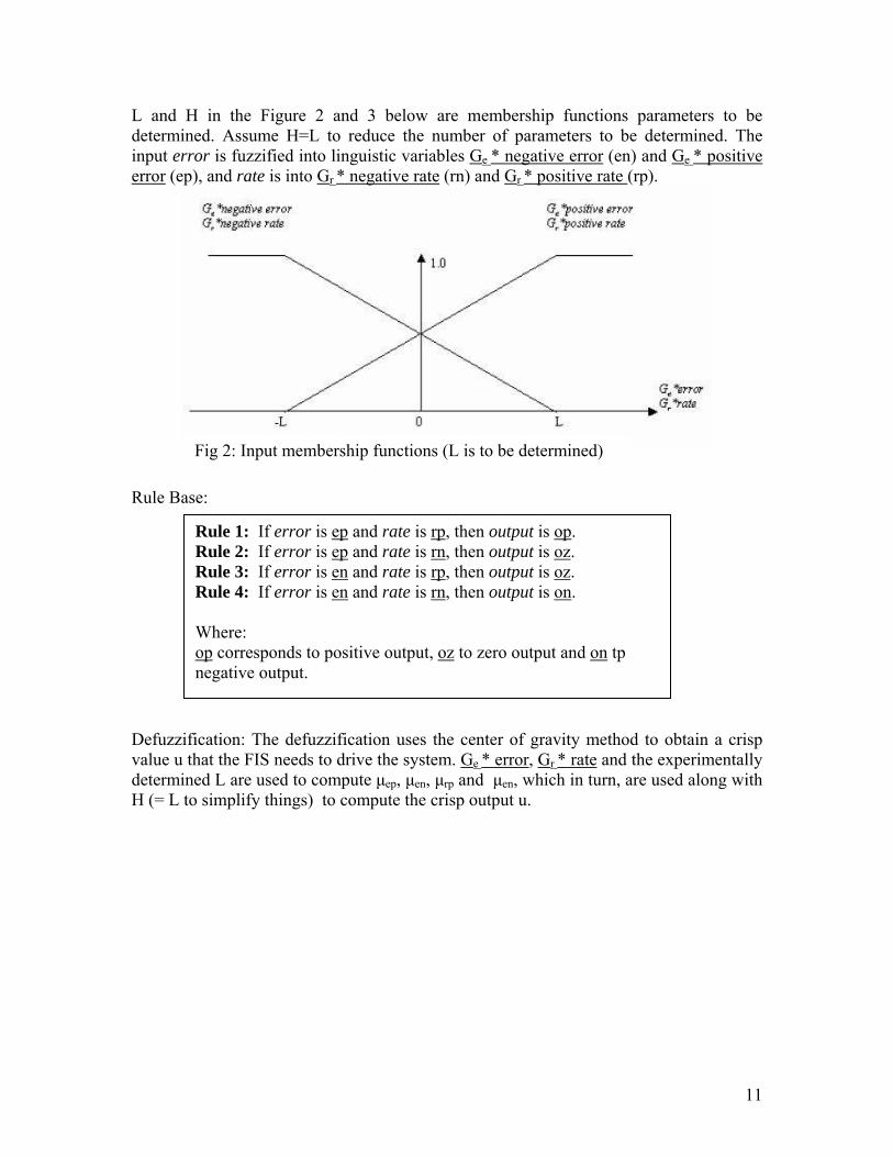
L and H in the Figure 2 and 3 below are membership functions parameters to be determined. Assume H=L to reduce the number of parameters to be determined. The input error is fuzzified into linguistic variables Ge * negative error (en) and Ge * positive error (ep), and rate is into Gr * negative rate (rn) and Gr * positive rate (rp).

Fig 2: Input membership functions (L is to be determined) Rule Base:

Rule 1: If error is ep and rate is rp, then output is op. Rule 2: If error is ep and rate is rn, then output is oz. Rule 3: If error is en and rate is rp, then output is oz. Rule 4: If error is en and rate is rn, then output is on. Where: op corresponds to positive output, oz to zero output and on tp negative output.

Defuzzification: The defuzzification uses the center of gravity method to obtain a crisp value u that the FIS needs to drive the system. Ge * error, Gr * rate and the experimentally determined L are used to compute μep, μen, μrp and μen, which in turn, are used along with H (= L to simplify things) to compute the crisp output u.

11

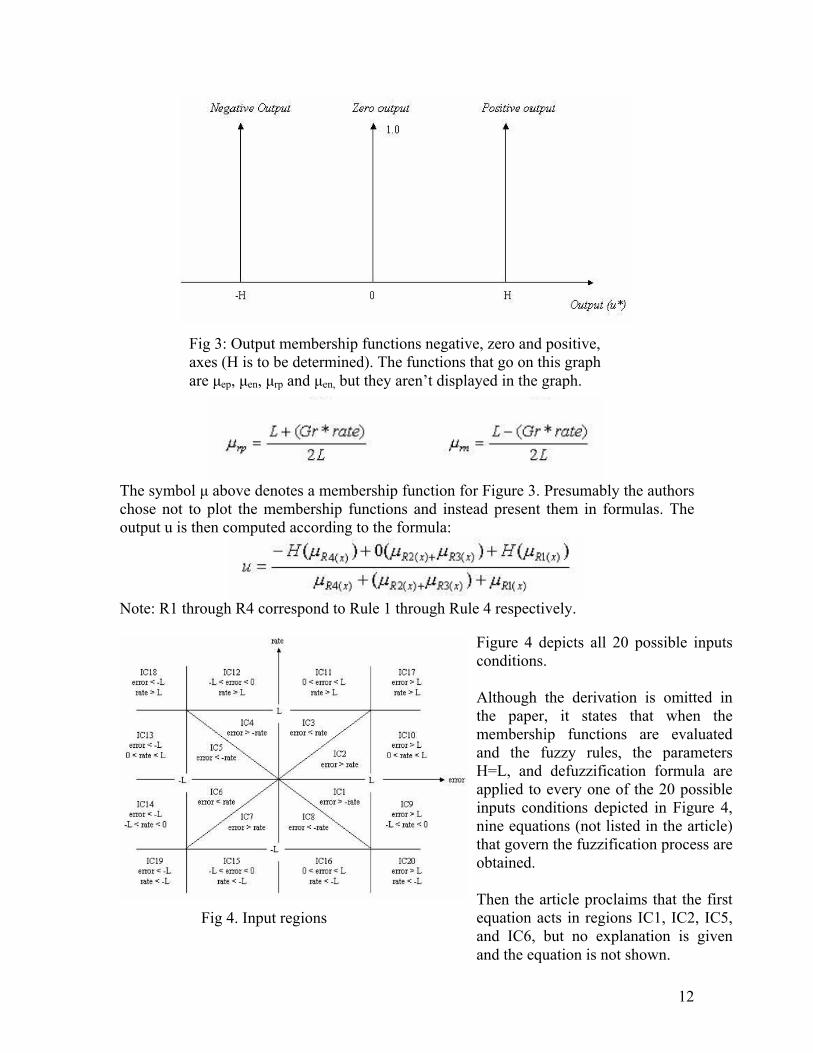
Fig 3: Output membership functions negative, zero and positive, axes (H is to be determined). The functions that go on this graph are μep, μen, μrp and μen, but they aren’t displayed in the graph.

The symbol μ above denotes a membership function for Figure 3. Presumably the authors chose not to plot the membership functions and instead present them in formulas. The output u is then computed according to the formula:

Note: R1 through R4 correspond to Rule 1 through Rule 4 respectively.

Fig 4. Input regions

12

Figure 4 depicts all 20 possible inputs conditions. Although the derivation is omitted in the paper, it states that when the membership functions are evaluated and the fuzzy rules, the parameters H=L, and defuzzification formula are applied to every one of the 20 possible inputs conditions depicted in Figure 4, nine equations (not listed in the article) that govern the fuzzification process are obtained. Then the article proclaims that the first equation acts in regions IC1, IC2, IC5, and IC6, but no explanation is given and the equation is not shown.

With the design of the FIS completed, Matlab’s Simulink is then used to implement the system.

Fig. 5 Tracking System implemented in Simulink Analysis of article: The inputs fuzzification membership functions are all trapezoidal. The exposition of the defuzzification process is very convoluted, making it difficult to extract the essence. Simply put, the defuzzification technique used is the center of gravity method, a method that reflects the location and shape of the fuzzy sets concurrently [9]. The paper is noteworthy for its demonstration of FPD as another viable fuzzy inference system and implementing a system in Simulink, a tool in Matlab that provides the users with a graphical interface for drawing the schematic of a process and running simulations. The fuzzy logic toolkit is designed to work seamlessly with Simulink; a FIS designed using the fuzzy logic toolkit can be directly embedded into a Simulink program [12]. The FPD is deemed useful by the authors for error detection and correction, and is very applicable to experiments with multiple sessions where errors may accumulate quickly.

13

2.1.3 Case Study III: Motion Tracking and Prediction “MOTION TRACKING AND PREDICTION SYSTEM UTILIZING IMAGE PROCESSING AND ARTIFICIAL INTELLIGENCE TECHNIQUE” Authors: K.B. How and K.B. See of Monash University, Malaysia Publication: http://digital.ni.com/worldwide/singapore.nsf/web/all/3838108CC968A0DB8625703D004ADAA5 Summary of Article: It designs a planar motion tracking and prediction system for a bright color object on dark background. The paper details the image acquisition and processing steps taken before any FIS is done. The paper concludes that fuzzy logic can be used for motion tracking and prediction. Hardware: USB webcam (30 fps, banding filter frequency 60 Hz), P4 2.0 Ghz PC w/ 512 RAM, toy vehicle with 150 mm/s speed. Software: LabVIEW 7.1, Creative Webcam Live Pro, NI-USB, NI-IMAQ Vision 7.1, PID Control Toolset Since our project, to a large extent, is also an exploration of image acquisition and processing, these aspects of the article are shown below for closer examination along with the fuzzy algorithms.

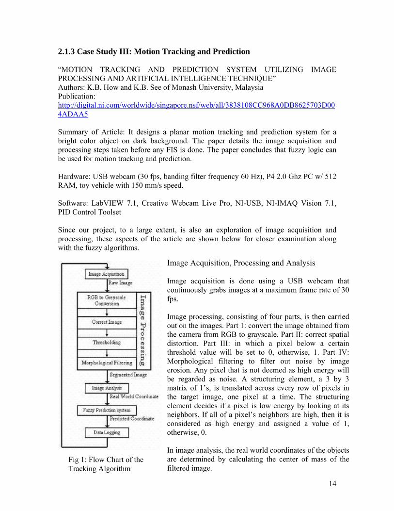
Image Acquisition, Processing and Analysis Image acquisition is done using a USB webcam that continuously grabs images at a maximum frame rate of 30 fps. Image processing, consisting of four parts, is then carried out on the images. Part 1: convert the image obtained from the camera from RGB to grayscale. Part II: correct spatial distortion. Part III: in which a pixel below a certain threshold value will be set to 0, otherwise, 1. Part IV: Morphological filtering to filter out noise by image erosion. Any pixel that is not deemed as high energy will be regarded as noise. A structuring element, a 3 by 3 matrix of 1’s, is translated across every row of pixels in the target image, one pixel at a time. The structuring element decides if a pixel is low energy by looking at its neighbors. If all of a pixel’s neighbors are high, then it is considered as high energy and assigned a value of 1, otherwise, 0. In image analysis, the real world coordinates of the objects are determined by calculating the center of mass of the filtered image.

14

Fig 1: Flow Chart of the Tracking Algorithm

Image Analysis using two cascaded fuzzy logic controllers The problem is broken up into two parts, each with a FIS of its own. Both FISs are “Mamdani” type and use equally positioned triangular membership functions and equally weighted rules. The inference method used is Min-Max. FIS I: Coarse Motion Prediction. This FIS obtains a coarse estimation of the motion of the object being tracked. Fuzzification: Angle (A) and the Angle Difference (dA) are inputs. A is fuzzified into S, m, or B, while dA is fuzzified into –B, -S, Z, +S, or +B. These italicized symbols represent linguistic variables such as “Big movement to the right” and “Small movement to the left”. The negative and positive presumably represent “left” and “right” respectively. Rule Base: The relationship between the inputs, the angle and angle difference, and the outputs, the magnitude and direction of the predicted move of the object, is summarized in Table 1. For example, if A is B and dA is +B, then predicted displacement is –M, or in other words, if the object has been moving very dynamically (as characterized by large A and dA), then there is going to be more object movement between the current image and the next.

Table 1: Rules for FIS I

Defuzzification: Not yet, as FIS II needs fuzzy inputs anyway. It is a waste of time to defuzzify the result now only to fuzzify it again in the next step. Therefore, there is no crisp output at this point. Note: it is erroneous to think of the output in its current state as only one linguistic variable as the output has some degree of affinity to all of the output membership functions, –L, -M, Z, +M, +L, at the same time. Instead think of each output as possessing of an array of degrees of affinity, but some maybe zero. FIS II: Fine Motion Prediction. To accomplish fine motion prediction, FIS II, shown in Table 2, provides a means for error correction. To this end, FIS II uses the output from the first and the error from the last session as inputs to produce the amount of fine step as output.

15

Fuzzification: Predicted magnitude of motion (Δc) and prediction error (ex) as inputs. Δc is still a fuzzy aggregate and no need further fuzzification. On the other hand, ex has to be fuzzified into linguistic variables –B, -S, Z, +S, +B. Rule Base: Summarized in Table 2. For example, if the prediction error is towards left, the prediction should be more towards right.

Table 2: Rules for FIS II Defuzzification: The center of gravity method, also known as the center of area method—a terminology preferred by some as stuff in the computer has no real mass. Data Logging When the tracking algorithm is executed, all data will be stored into an array temporarily. Upon termination of the tracking algorithm, these arrays will be written to a text-file. Through out the tracking algorithm, the real world x and y coordinates, predicted x and y coordinates, and timing of each frame are logged for evaluation of the system performance. Analysis of article: As this research is similar in some regard to what we are doing, there is much of the set-up that provides useful insight. We both use bright objects on darker background and cheap USB webcams. A big difference is in the choice of software. Our choice, Matlab fuzzy logic toolkit, allows for quick customization of fuzzy inference system and this affords us experimentation that would not be otherwise possible. Furthermore, Matlab is more readily available to us than LabVIEW. LabView and Matlab Fuzzy Logic Toolkit are both graphical tools designed for use by programmers and non-programmers alike.

16

While the location of each object in the article is computed using the weighted averages of its center of mass, this will not suffice for tracking multiple objects with complex identification patterns like ours. Instead of using weighted averages, we shall build a FIS for determining the direction an object is facing and its identity. The paper uses cascaded FIS and makes the FIS design process less of a headache as the problem is broken down to more manageable parts. The first FIS shown in the paper computes the future object location. The second adjusts for error. This brings to mind the two-part nature of our project: the position tracking part and the identification part, so our system can certainly benefit from a two-FIS dynamic of this sort. Implementing a cascaded FIS simply means using the output of one FIS as inputs to the next. So the result from the FIS for computing object direction is not the final result, instead it drives the second FIS that computes the object’s id—the ultimate output.

17

2.1.4 Case Study IV: Urban Canyon Vehicle Navigation “MAP MATCHING ALGORITHM FOR VEHICHLE NAVIGATION SYSTEM IN URBAN CANYONS” ARTICLE Authors: S. Syed and M.E. Canon of University of Calgary, Canada Publication: Presented at ION National Technical Meeting, San Diego 2004 Link: http://plan.geomatics.ucalgary.ca/papers/04ntmsalman_footers.pdf Summary of article: They developed a high-tolerant map-matching algorithm using fuzzy logic (FL), a widely noted soft computational method with inherent tolerance for imprecise input. In vehicle navigation, map matching is used to constraint the position of a vehicle on the road network map. The FL map-matching algorithm will work hand in hand with High Sensitivity Global Positioning System (HSGPS), which has errors that are difficult to model when operating in urban canyons location due to various interference effects. FL will generate precise output from the noisy navigation input obtained from the HSGPS. The paper concludes that the reliability of the algorithm using FL far exceeds that of a conventional algorithm based on geometric approach. It shows that FL is a low cost solution to navigational map matching and details the two fuzzy inference systems (FIS) used.

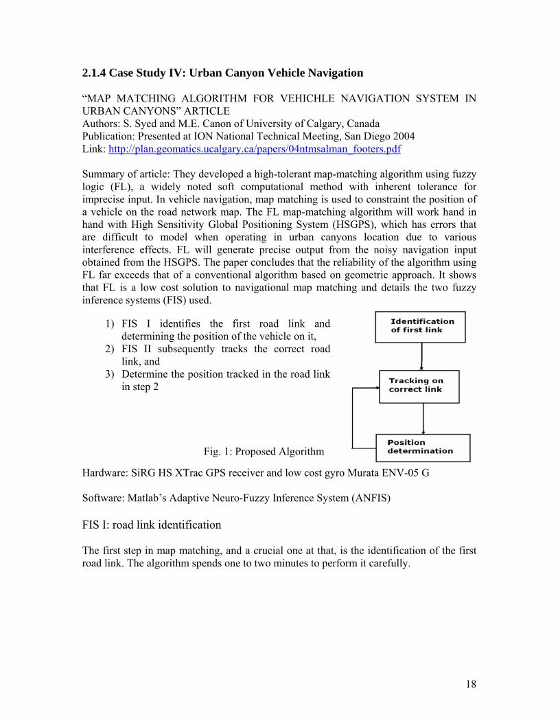
1) FIS I identifies the first road link and determining the position of the vehicle on it,

2) FIS II subsequently tracks the correct road link, and

3) Determine the position tracked in the road link in step 2

Hardware: SiRG HS XTrac GPS receiver and low cost gyro Murata ENV-05 G

Fig. 1: Proposed Algorithm

Software: Matlab’s Adaptive Neuro-Fuzzy Inference System (ANFIS) FIS I: road link identification The first step in map matching, and a crucial one at that, is the identification of the first road link. The algorithm spends one to two minutes to perform it carefully.

18

Membership functions

Fig 2: FIS for first road link identification (simplified)

Fuzzy Inputs: a) Distance of the position output from the

links b) Velocity direction with respect to road

links c) Heading change (obtained from the gyro) d) Time (obtained from GPS)

Fuzzy Sets:

1) Nominal heading change 2) Belongingness to a close link set 3) Similarity of velocity direction and link

orientation 4) Large number of epochs

19

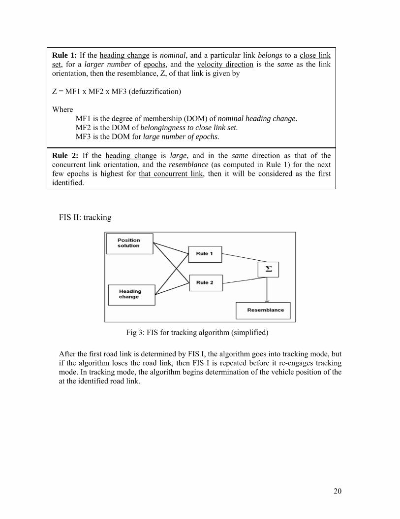
Rule 2: If the heading change is large, and in the same direction as that of the concurrent link orientation, and the resemblance (as computed in Rule 1) for the next few epochs is highest for that concurrent link, then it will be considered as the first identified.

Rule 1: If the heading change is nominal, and a particular link belongs to a close link set, for a larger number of epochs, and the velocity direction is the same as the link orientation, then the resemblance, Z, of that link is given by Z = MF1 x MF2 x MF3 (defuzzification) Where MF1 is the degree of membership (DOM) of nominal heading change. MF2 is the DOM of belongingness to close link set. MF3 is the DOM for large number of epochs.

FIS II: tracking

Fig 3: FIS for tracking algorithm (simplified) After the first road link is determined by FIS I, the algorithm goes into tracking mode, but if the algorithm loses the road link, then FIS I is repeated before it re-engages tracking mode. In tracking mode, the algorithm begins determination of the vehicle position of the at the identified road link.

20

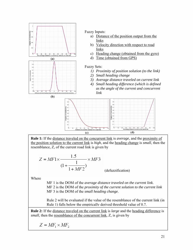
Fuzzy Inputs: a) Distance of the position output from the

links b) Velocity direction with respect to road

links c) Heading change (obtained from the gyro) d) Time (obtained from GPS)

Fuzzy Sets:

1) Proximity of position solution (to the link) 2) Small heading change 3) Average distance traveled on current link 4) Small heading difference (which is defined

as the angle of the current and concurrent link

Rule 2: If the distance traveled on the current link is large and the heading difference is small, then the resemblance of the concurrent link, Z, is given by

Rule 1: If the distance traveled on the concurrent link is average, and the proximity of the position solution to the current link is high, and the heading change is small, then the resemblance, Z, of the current road link is given by

Where MF 1 is the DOM of the average distance traveled on the current link. MF 2 is the DOM of the proximity of the current solution to the current link MF 3 is the DOM of the small heading change.

Rule 2 will be evaluated if the value of the resemblance of the current link (in Rule 1) falls below the empirically derived threshold value of 0.7.

(defuzzification)

21

Analysis of article: ANFIS uses Takagi-Sugeno-Kang, or simply Sugeno, fuzzy rules. Sugeno-type FIS is the same as Mamdani in all regard except that the Sugeno output membership function is either linear or constant [12]. Matlab ANFIS comprises of four parts: the first two are fuzzification and predicate rules, the third is Sugeno rule, and the last is defuzzification using weighted global output [8]. However, the methodology used in the article differs on two counts: the output Z (resemblance) does not appear to be linear and the defuzzification is done using proprietary formulas instead of the weighted global output. Nonetheless, ANFIS’ backpropagation and least square optimization technique are used for the optimization of membership functions. Backpropagation modifies the initially chosen membership functions while the least mean square algorithm determines the coefficients of the linear output functions [8]. It seems advantageous to follow in this article’s footsteps and employ Matlab’s ANFIS for the motion tracking and prediction system, especially since the initial build was already done using Matlab fuzzy toolkit and it is designed to work seamlessly with ANFIS. A possible barrier to using ANFIS is the fact that the output membership function must be Sugeno-type. Also note worthy is the fact that the second FIS in the article has two rule bases, which it selects depending on the situation. Such dual-mode design is very handy and may be adapted for our purposes.

22

2.2 Comparison of Case Studies Case Study 1: Small Engine Control by Fuzzy Logic Case Study 2: Fuzzy Condensed Algorithm Applied to Control a Robotic Head for Visual Tracking Case Study 3: Motion Tracking and Prediction System Utilizing Image Processing and Artificial Intelligence Technique Case Study 4: Fuzzy logic based map matching algorithm for vehicle navigation system in urban canyons

Table of Methodology Fuzzification Fuzzy Inference

System Defuzzification

CS 1: SMALL ENGINE CONTROL

Mamdani, Trapezoidal MFs

Mamdani Singleton

CS 2: ROBOT HEAD Mamdani Mamdani, Fuzzy Proportional Derivative

Centroid

CS 3: MOTION TRACKING & PREDICTION SYSTEM

Mamdani, equally positioned triangular MFs

Mamdani, Cascaded “Min-Max” FIS, equally-weighted rules

Centroid

CS 4: VEHICLE NAVIGATION

Mamdani, a variety of MFs (Gaussian, step, sigmoid, linear)

Sugeno, Adaptive Neuro Fuzzy Inference System

Custom formula

THIS PROJECT Mamdani Mamdani, Cascaded Adaptive Neuro Fuzzy Inference System

Centroid

Learning from past research provides some insight into the different paths once can take in the design of a fuzzy inference system (FIS). The case studies have shown us various membership function shapes. We selected trapezoidal, Gaussian and triangular for our purposes. Either trapezoidal or Bell function is appropriate when a specific degree of affinity has a wide range. The trapezoidal function can be replaced by any function that plateaus, such as the latter. The Gaussian and triangular shapes are appropriate when there is only one maximum degree of affinity. There is more to discuss here, such as what parameters to use, which will be discussed later. Case studies 2 and 3 have shown us that Adaptive Neuro Fuzzy Inference System (ANFIS) and Fuzzy Proportional Derivative (FPD) are useful for optimization. Our experimentation with ANFIS will be shown in the later chapters detailing various

23

optimization attempts. Unfortunately, we will not have the time to explore FPD at great length. Cascading smaller FIS, as in case study 3, is an alternative to having a single, bigger FIS. We would rather break a problem down into several parts and tackle each part separately. Due to the difficulties involved in transferring a fuzzy variable from one FIS to the next, it has to be defuzzified first and then fuzzified again. The choice between Mamdani and Sugeno type FIS depends on the type of inputs. Mamdani is more suited for intuitive, human inputs while Sugeno works well with linear inputs [12] like those for the PID control in case study 2. The Sugeno type is a more computationally efficient system that lends itself well to the use of adaptive models [12], such as the ANFIS that is shown in case study 4, but it’s also a more compact system that imposes a lot of constraints on the FIS. In light of all of this, we decided to use Mamdani-type whenever possible. Unfortunately, we have not been able to learn much about rule drafting from the case studies; they don’t discuss how they came up with the rule base since it would be a long discussion. Rule drafting is a difficult process that requires an expert knowledge of the real world system being modeled, which in our case means knowing the appearance of bright objects on dark background in various orientations and degrees of distortion. Defuzzification is a tricky process that requires much thought and experimentation. The difficulty is in coming up with a formula or function that translates the outcome of the rules into one or more crisp values. The decision to use a centroid (CoG) method or a weighted global output method has to be made and the defuzzification MFs have to be designed from scratch just like the fuzzification MFs. For centroid defuzzification, the output is obtained by integrating across the MFs [12]. The centroid method is usually essential for Mamdani-type systems, unless single-spikes, a.k.a. singletons, MFs are used [12] as in case study 1. For Sugeno-type systems, the commonly used defuzzification method is the weighted global output method, which involves taking the weighted average of a few data points [12]. Suffice it to say for now that during the defuzzification of our FISs, weighted global output is used for Sugeno-type FIS and centroid is used for Mamdani-type FIS. Fortunately, field testing is not something that we have to worry about. Instead, we test our system in the lab by using our own test suites. Case study 2 described using Mathwork’s Simulink in detail. Simulink is a great tool for the purpose of simulating a FIS coded using Matlab.

24

Chapter 3: Hardware and Software In order to acquire data on the objects, we took pictures of them using a web cam. This required fixed lighting and camera angle. To facilitate this, a worktable is built that has an overhead frame where the lights and camera are installed. The camera is hooked up to a computer where the images are processed and analyzed. Our lab computer is rather backwards but we make do. We programmed the image acquisition, processing and the fuzzy expert systems using Matlab with three specialized toolboxes that will soon be explained in greater details. 3.1 Worktable Dimension: 2.3 x 1.2 m Height: 1 m from the floor to table surface 1.3 m from the table surface to the table ceiling The ceiling has three lights: two at the sides and one right at the center near the camera. The table surface is covered with gray carpet to reduce light reflection. 3.2 Computer Specifications: Pentium Celeron 2.2 GHz, 256 MB RAM, Windows XP The lab computer is rather inadequate for this project as the recommended requirement for running Matlab is a Pentium III processor with 512 MB RAM. Although the one of the goals of our project is to simplify a position tracking problem using fuzzy logic so our solution can run on slower computers, the image acquisition and processing are very computationally expensive. Nevertheless, we have accomplished much using it. Instead of feeding a video into the system, as we originally intended, the system processes one image at a time. 3.3 Camera Model: Creative Live! Ultra Specifications: Wide angle lens, 1.3 Mega Pixels, 640 x 480 resolutions video at 30 fps We purchased an economical, wide-angle web camera for the project to intentionally introduce the problem of noise. The camera is positioned directly above the center of the worktable. The wide angle is necessary for capturing the entire table surface. Although the camera captures video up to 30 fps, the limited processing speed of the lab computer only enables us to capture video at approximately 20 fps.

25

3.4 Matlab The image acquisition software provided by Creative is very good, but we chose to use Matlab’s Image Acquisition Toolbox to write our own routine. This allows us to make certain adjustments to the images as we see fit. After the images are acquired successfully and ready for processing, we use the Image Processing Toolbox to perform linear filtering on them. Again, we wrote a routine to handle the task. Finally, when we have sufficient data from each image, we use the Fuzzy Logic Toolbox to help us ascertain the directions the objects in the image are facing and their IDs. All this will be discussed in further details in the next few chapters.

26

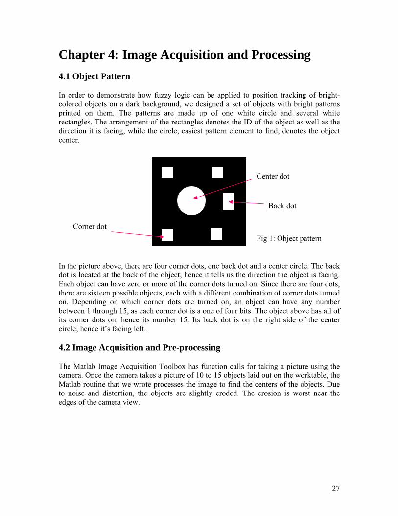
Chapter 4: Image Acquisition and Processing 4.1 Object Pattern In order to demonstrate how fuzzy logic can be applied to position tracking of bright-colored objects on a dark background, we designed a set of objects with bright patterns printed on them. The patterns are made up of one white circle and several white rectangles. The arrangement of the rectangles denotes the ID of the object as well as the direction it is facing, while the circle, easiest pattern element to find, denotes the object center.

Center dot

Back dot

Corner dot Fig 1: Object pattern

In the picture above, there are four corner dots, one back dot and a center circle. The back dot is located at the back of the object; hence it tells us the direction the object is facing. Each object can have zero or more of the corner dots turned on. Since there are four dots, there are sixteen possible objects, each with a different combination of corner dots turned on. Depending on which corner dots are turned on, an object can have any number between 1 through 15, as each corner dot is a one of four bits. The object above has all of its corner dots on; hence its number 15. Its back dot is on the right side of the center circle; hence it’s facing left. 4.2 Image Acquisition and Pre-processing The Matlab Image Acquisition Toolbox has function calls for taking a picture using the camera. Once the camera takes a picture of 10 to 15 objects laid out on the worktable, the Matlab routine that we wrote processes the image to find the centers of the objects. Due to noise and distortion, the objects are slightly eroded. The erosion is worst near the edges of the camera view.

27

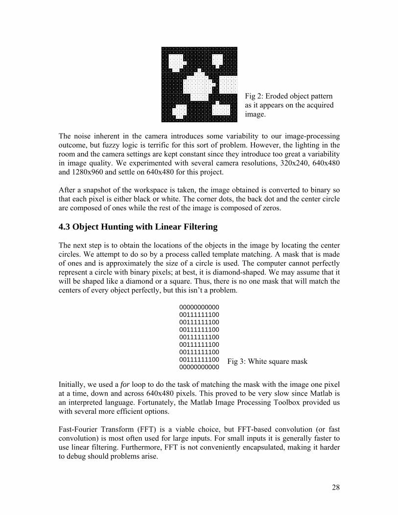
Fig 2: Eroded object pattern as it appears on the acquired image.

The noise inherent in the camera introduces some variability to our image-processing outcome, but fuzzy logic is terrific for this sort of problem. However, the lighting in the room and the camera settings are kept constant since they introduce too great a variability in image quality. We experimented with several camera resolutions, 320x240, 640x480 and 1280x960 and settle on 640x480 for this project. After a snapshot of the workspace is taken, the image obtained is converted to binary so that each pixel is either black or white. The corner dots, the back dot and the center circle are composed of ones while the rest of the image is composed of zeros. 4.3 Object Hunting with Linear Filtering The next step is to obtain the locations of the objects in the image by locating the center circles. We attempt to do so by a process called template matching. A mask that is made of ones and is approximately the size of a circle is used. The computer cannot perfectly represent a circle with binary pixels; at best, it is diamond-shaped. We may assume that it will be shaped like a diamond or a square. Thus, there is no one mask that will match the centers of every object perfectly, but this isn’t a problem.

00000000000 00111111100 00111111100 00111111100 00111111100 00111111100 00111111100

Fig 3: White square mask 00111111100 00000000000

Initially, we used a for loop to do the task of matching the mask with the image one pixel at a time, down and across 640x480 pixels. This proved to be very slow since Matlab is an interpreted language. Fortunately, the Matlab Image Processing Toolbox provided us with several more efficient options.

Fast-Fourier Transform (FFT) is a viable choice, but FFT-based convolution (or fast convolution) is most often used for large inputs. For small inputs it is generally faster to use linear filtering. Furthermore, FFT is not conveniently encapsulated, making it harder to debug should problems arise.

28

Linear filtering is a technique for enhancing an image. It can be used for template matching. The image processing toolbox has functions that can perform linear filtering using either correlation or convolution. Convolution will rotate the mask 180 degrees but correlation will keep it the same. It actually doesn’t matter for the mask shown in Figure 3, but we picked correlation to avoid complications should we decide to change the mask. 4.4 Weeding Out Aliases After we carried out linear filtering, an energy map of the image is obtained. Unlike the original, the energy map will not show binary pixels as pixels change gradually from low to high energy, depending one their neighbors. The energy map contains the information that we need to locate the object center. The center of the object has the highest value on the energy map, so by finding the highest value on the map, we have also found the object center.

Fig 5: The appearance of an object on the energy map.

If we compare the original image to the energy map, we will see that at the location of an object in the original image, the energy map will have a clump of energy at the same location. If the mask is well designed, the location of the highest energy in a cluster of energy is the location of an object center in the original image. Thus, we have to find the local maxima of the energy map to find all the object centers in the original image. However, the presence of noise complicates matters. Even noise that is one pixel big is its own local maximum. Thus we need to set a threshold to weed out potential false positives. It’s difficult to determine the right threshold value for the entire energy map since the distortion due to the camera is non-uniform. Objects further from the center of the table tend to be more eroded and appear weaker on the energy map even though they are actual objects, not noise. Consequently, the threshold value cannot be set too high. The goal is to have one positive match per object. No more, certainly no less. To achieve this, we combined all of the method discussed in the above. First, we experimentally determined a threshold value to eliminate small energy clusters. Next we find the local

29

maxima of the remaining clusters of energy. Finally, we use a for loop to go through the high energy pixels and take only one from each group of high pixels (because if they are grouped together then they are probably from the same object), thus obtaining one high energy pixel per object. 4.5 Stat Array The next step involves predicting the motion of the objects as this will help reduce the search space of subsequent position tracking. Although the process above determined where the object centers are, we still do not have all of the information we need for motion prediction. That requires knowledge the object’s orientation. Hence, we have to look for the back dot. To make the best of the energy map, we will use it to help us find the back dot. The energy map was originally designed to help us locate the center dot, so we need to make a few modifications. The back dot is in close proximity with the center. Since we already know the center of each object, we only need to do a little work to find the back dot. Or so we thought. Finding the back dot is not easy because it’s not very different from a corner dot. We have to use fuzzy logic to help us, but first we need to come up with a set of inputs to the fuzzy inference system. From the distribution of energy in an energy map, we can the orientation and the ID of the corresponding object. The distribution is summarized by the stat array, which is a 3x3 matrix of the energy map nine regional means. If we compute the differences between opposite ends of the center region of the stat array, meaning if we find the difference between the upper left region and the lower right, upper right and lower left region, upper middle and lower middle, and center left and center right region, we will have four numbers that could help us pinpoint the direction the object is facing. These four are the major slopes. One of the goals of this project is to build a fuzzy logic system that takes as few inputs as possible. This ensures that the system is as efficient and as computationally inexpensive as it can be. We have reduced the data from 21x21 (441 values) to just four.

Lower right

Lower left

Upper right

Upper left

Center right

True center

Center left

Upper middle

Lower middle

Fig 6: Stat array of an object (each cell contains the regional mean)

Going back to Figure 5, one should perceive a circle at the center and several rectangles surrounding it. Some objects energy patterns, like this one, are easier to interpret than others. Whether one can successfully guess how the original looks like from an energy

30

map depends on the quality of the original image and how confusing the dot arrangement is. Image erosion that occurs during image acquisition is non-uniform across an object and since we rely on the proportion of the object elements in the original image to guide us, the severity of the distortion will directly affect the accuracy of our guesses. Our example so far is an easy one because its orientation is fairly obvious; the back dot is obvious: it’s the dot that has no dot on the other side of the center circle. In other words, the largest major slope is much bigger than the other three. However, many objects are not that simple. Figure 7 depicts the energy map of object number 3 facing down. For this object, it’s not as easy as before to tell which energy cluster belongs to the back dot. One may observe that the upper left region is the second strongest and therefore that must be the back dot. Although in theory, we could simply normalize the energy levels of the region to pinpoint the back dot, the distortion caused by our web camera deprives us of such an easy solution.

Fig 7: The energy map of object no. 3 facing down.

Using correlation, we know where the object is but we still do not know its orientation and ID. The regional means computed and stored in the stat array should have been sufficient for identifying the object number and orientation, but the problem is confounded by distortion caused by the camera. We have described how we acquired and processed images containing object patterns. More importantly, we have shown how the data that we got is reduced to only four numbers per object. Next, we will describe how we applied the fuzzy logic techniques, introduced in the preceding chapters, to ascertain the orientation and ID of each object.

31

32

Chapter 5: Position Tracking Fuzzy Logic System 5.1 Expert Knowledge A challenging stage in the design of a fuzzy logic expert system involves imbuing human expertise onto a set of rules to be fed to the fuzzy logic system. In industries, this is done by interviewing experts or bringing them in as consultants. However, the uniqueness of our problem means that we can solicit advice from very few people, if any. In the hopes that we ourselves become sufficiently expert at position tracking, we performed careful analysis the object energy data and conducted a study of people with science background to find out how they interpret the data and what rules they would come up with. 5.1.1 Analysis of Object Energies The previous chapter details how the rectangles and circle show up on an energy map and how this map is broken up into nine regions. Using the stat array, the fuzzy logic system should be able to know what object it is and what direction it is facing just like a human expert could, based on rules that govern the energy pattern of 15 different objects in 16 possible orientations. Just as the stat array is a summary of the energy pattern of an object, the major slopes are a summary of the stat array. Studying how different objects and orientations affect the major slopes will help us create the rule base that will let us discern an object’s ID and direction from its energy map.

0.059 0.044

0.034 0.063

0.099 0.139 0.034

0.032

0.047

Fig 1: Stat Array of Object 15 facing left with bleed over from the center dot.

The above stat array shows the region means of object 15 facing left. Object 15 has four corner dots, one back dot located in middle right region, and a center circle. Although there are no dots in the upper center, middle left and lower center regions, the energy at those regions is as high as the corner regions. Thus, it is difficult to tell from the stat array above whether or not the corner regions have dots. It turns out that there is a significant energy bleed over particularly from the center region with the large circle to other regions. Furthermore, the bleed over only occurs between adjacent regions. Therefore, the presence of the large center circle in the center region affects only the upper middle, middle left, middle right and lower center regions causing them to be as high as the corner regions. Since the purpose of the center dot is to help find the object, it has now outlived its usefulness and can be removed so as to reduce bleed over. Figure 2 shows the same object with the center dot removed.

33

0.058 0.043

0.033 0.062

0.082 0.021 0.016

0.024 0.035

Fig 2: Stat Array of Object 15 facing left with center dot removed.

With the center dot removed, the corner regions have higher energies than the side regions for the most part (the upper right region contains a dot but for some reason it’s dimmer than usual). The four major slopes may now computed in the following way:

Lower right (LR)

Lower center (LC)

Lower left (LL)

Middle right (MR)

Middle Center (MC)

Middle left (ML)

Upper right (UR)

Upper center (UC)

Upper left (UL)

Fig 3: Computing the four major slopes removed.

Major Slopes Computation ML-MR = 0.016 – 0.082 ≈ -0.07 UC-LC = 0.024 – 0.035 ≈ -0.01 UL-LR = 0.062 – 0.058 ≈ -0.00 UR-LL = 0.033 – 0.043 ≈ -0.01 The major slopes are then normalized to reduce the effect of uneven lighting and distortion across the worktable. This is also done so that the range of values of inputs to the fuzzy inference system is more or less constant across objects. Normalized Major Slopes ML-MR = -1.00 UC-LC = -0.18 UL-LR = 0.07 UR-LL = -0.14 From the study of major slopes of all the objects (1-15) in various orientations, we created a set of guidelines for determining the object orientation. For example, if UC-LC is small in magnitude and ML-MR is a big negative value, then the back dot is most likely in the middle right region and therefore the object is facing leftwards.

34

5.1.2 Measuring Human Performance To further our understanding of the problem, we conducted a study where human subjects with Science or Mathematics background will try to solve the problems described above. The objective is two-fold: To anticipate the difficulties that the fuzzy expert system may encounter and to learn new ideas by observing how others deduce the orientation and ID of an object from its energy map. We obtained five test subjects and conducted two experiments over the course of two weeks. The first experiment aimed to measure the their ability at guessing the direction and ID of objects from energy maps (441 data points per object), and also acquaint them with fuzzy logic and the problem at hand. To do so, we selected 16 relatively straightforward object patterns for them to analyze individually in one hour. The subjects are instructed to write or draw how they think each object looks like (how many corner dots are on and how it is oriented) and list the rules that their conclusions are based on. They were also to rate each question on a scale of 1 through 10 to collectively sum up the uncertainty in their answer and the difficulty of the question, so if an energy map is very difficult to interpret and they’re unsure of their answer, then it should be given a high rating. The second experiment aimed to measure their ability to perform the same task but using the stat array (9 data points per object), and a few of the object patterns we selected for this are relatively more baffling than before. A summary of the results of the experiments will be shown at the end of this chapter. 5.2 Direction Fuzzy Inference System Once we became experts in discerning objects’ orientation and ID, we proceeded to design the fuzzy inference system that will do just that. The first step was to decide what the inputs to the system would be. The four major slopes are suitable as inputs because they can tell you the location of the back dot. The output is obvious: the direction the object is facing, but how it should be represented in the system requires careful consideration. The output cannot be represented as degrees because the resulting function is not circular and the system will break. At times, the direction of the object cannot be precisely determined. Should the need to average two or more likely directions arise, the system may not produce the correct output. For example, if system thinks that NW (315º) and NE (45º) are the two likely directions, the inference system then deduces that the correct direction is S (180º) instead of N (0º) because S (180º) is the average of the two. Therefore, we use eight direction vectors to represent the output instead. To resolve this problem, we developed a novel resultant vector defuzzification method. In this approach, each possible answer is considered to be a vector and the final answer is the calculated resultant vector. The heart of this project, the fuzzy inference system, will be explained in three parts: the fuzzification, rule base and the defuzzification.

35

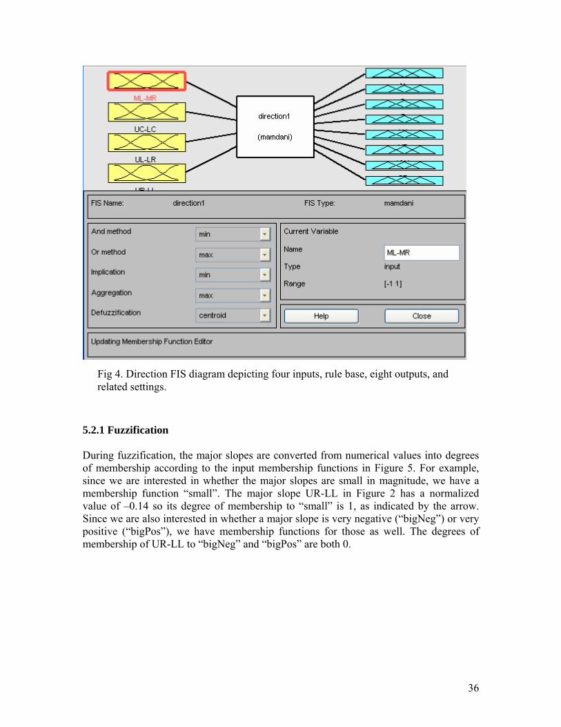
Fig 4. Direction FIS diagram depicting four inputs, rule base, eight outputs, and

related settings. 5.2.1 Fuzzification During fuzzification, the major slopes are converted from numerical values into degrees of membership according to the input membership functions in Figure 5. For example, since we are interested in whether the major slopes are small in magnitude, we have a membership function “small”. The major slope UR-LL in Figure 2 has a normalized value of –0.14 so its degree of membership to “small” is 1, as indicated by the arrow. Since we are also interested in whether a major slope is very negative (“bigNeg”) or very positive (“bigPos”), we have membership functions for those as well. The degrees of membership of UR-LL to “bigNeg” and “bigPos” are both 0.

36

Fig 5. Membership functions for input fuzzification; Y-axis: degree of membership; X-axis: crisp input

Choosing the type of membership functions is difficult because the options are limitless. The membership functions above are selected because they are best suit the task at hand. For the “small” membership function, a Gaussian-Bell curve is selected because smoothness and symmetry are required to realistically model the change in the degree of membership to said property. The “bigNeg” and “bigPos”, on the other hand, are high on one side only so the two polynomial based curves, Z and S (both named because of their shapes), are used instead. Sigmoidal functions can be also be used here with similar effects. After we selected the shapes, we picked a reasonable set of parameters so we could proceed with the design of the rest of the inference system. The parameters of the membership functions determine which values are strong members so they have to be set correctly. However, only when the FIS as a whole is completed could the testing and tuning of the parameters begin proper. 5.2.2 Rule Base After the inputs are fuzzified, we apply the following rules:

1. If (ML-MR is small), (UC-LC is big neg), and (UL-LR is not big neg) then (E is high and everything else is not high). (Weight: 1)

2. If (ML-MR is big pos) and (UC-LC is small) then (S is high and everything else is not high). (Weight: 1)

3. If (UL-LR is small) and (UR-LL is big neg) then (output1 is SE), (output2 is S). (Weight: 1)

4. If (UL-LR is big pos), (UR-LL is small) and (ML-MR is not big neg) then (SW is high and everything else is not high). (Weight: 1)

5. If (ML-MR is big neg), (UC-LC is small), (UR-LL is not big neg), and (UL-LR is not big pos) then (N is high and everything else is not high). (Weight: 1)

6. If (UL-LR is small), (UR-LL is big pos) and (ML-MR is not big pos) then (NW is high and everything else is not high). (Weight: 1)

7. If (UL-LR is big neg), (UR-LL is small) and (ML-MR is not big pos) then (NE is high and everything else is not high). (Weight: 1)

37

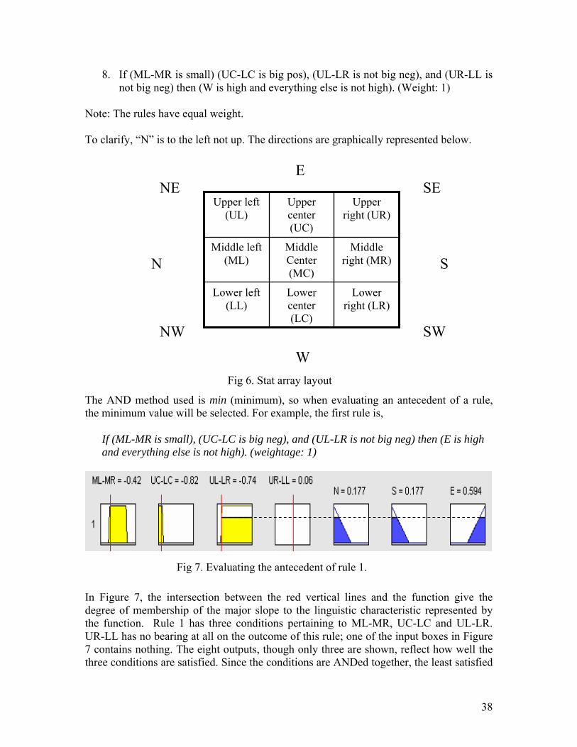
8. If (ML-MR is small) (UC-LC is big pos), (UL-LR is not big neg), and (UR-LL is not big neg) then (W is high and everything else is not high). (Weight: 1)

Note: The rules have equal weight. To clarify, “N” is to the left not up. The directions are graphically represented below. The AND method used is min (minimum), so when evaluating an antecedent of a rule, the minimum value will be selected. For example, the first rule is,

If (ML-MR is small), (UC-LC is big neg), and (UL-LR is not big neg) then (E is high and everything else is not high). (weightage: 1)

Lower right (LR)

Lower center (LC)

Lower left (LL)

Middle right (MR)

Middle Center (MC)

Middle left (ML)

Upper right (UR)

Upper center (UC)

Upper left (UL)

N S

E

W

SW

NE SE

NW

Fig 6. Stat array layout

Fig 7. Evaluating the antecedent of rule 1. In Figure 7, the intersection between the red vertical lines and the function give the degree of membership of the major slope to the linguistic characteristic represented by the function. Rule 1 has three conditions pertaining to ML-MR, UC-LC and UL-LR. UR-LL has no bearing at all on the outcome of this rule; one of the input boxes in Figure 7 contains nothing. The eight outputs, though only three are shown, reflect how well the three conditions are satisfied. Since the conditions are ANDed together, the least satisfied

38

condition governs all of the outputs, as indicated by the dotted line. The implication method used is also min (minimum) and it determines how antecedent affects the consequent, or outputs. The min implication method will truncate the output sets as depicted above. The same steps are performed on the rest of the rules. Then the rules are combined in the aggregation process, in which the truncated output functions returned by the implication process of each rule, all sixty-four of them (eight per rule), are combined into eight output fuzzy sets. The max aggregate method is used so the outputs are merely stacked on each other.

Fig 8. Aggregation of output fuzzy sets

Aggregation Results

5.2.3 Defuzzification

The final part of the fuzzy inference system converts the fuzzy result into eight direction vectors. Actually, the previous section has already outlined the defuzzification process step-by-step, from the implication to the aggregation stage. The result is the magnitudes of the direction vectors that if added together will produce the direction that the object is facing. These magnitudes are located at the top of Figure 8 next to their corresponding direction vector. Note that these magnitudes are crisp not fuzzy values. Since much of the defuzzification process has been explained, this section focuses on the membership functions used. The eight fuzzy outputs will be converted to crisp values in accordance with the three triangular membership functions, “low”, “med” and “high” in Figure 9.

39

Fig 9. Membership functions for output defuzzification; Y-axis: degree of membership; X-axis: crisp output

Figure 8 shows a combination of major slopes that satisfies rule 1 almost completely, and rule 7 just a little. So the consequence of rule 1 is asserted, but not those of the other rules. The consequence of rule 1 is: E (East) is “high” and all the rest are “low”. The fact that the consequence of rule 1 is asserted is reflected by the large amount of shaded area, denoted in blue, under the “high” function for the East direction vector and under the “low” function for the other direction vectors. The consequence of rule 7 is: NE is high and the rest are “low”. Since rule 7 is only satisfied to a small degree, the amount of blue under the “high” function for the NE direction vector and under the “low” function for the other direction vectors is small. As mentioned above, the aggregation process stacks the outputs together. So the aggregated E direction vector has some blue under the “low” function and a large amount of blue under the “high” function. The final defuzzification step is to compute the center of mass of the total shaded area under the “high” and “low” functions. This produces the crisp input E = 0.594 displayed at the top of Figure 8. The other direction vectors are computed the same way. 5.3 Object Rotation The purpose of object rotation is to make the task of identifying the object simpler. The idea is to rotate an object so that it faces leftward or north (0º), and then identify which of its corner dots are on. This is doable since the object orientation is already known in terms of direction vectors. The direction vectors are added together and then converted to degrees, and this is how much the object is rotated. 5.4 ID Fuzzy Inference System Fuzzy logic is employed once more to determine which dots are on. The inference system takes in the outward slopes, the slopes from the object center to the four corners plus the

40

back of the object in Figure 10, and outputs five crisp values that denote how strong the corner dots and the back dot are on. The outward slopes are computed using the original stat array, the one with the center dot. We could simply measure the energy level of a region to decide whether or not an outer dot is present, but in order to eliminate the effect of uneven distortion and pixel erosion across the worktable we need the difference between the center region and that region. Granted, the distortion across an object is a little uneven, but it’s relatively minor.

Lower right (LR)

Lower center (LC)

Lower left (LL)

Middle right (MR)

Middle Center (MC)

Middle left (ML)

Upper right (UR)

Upper center (UC)

Upper left (UL)

Fig 10: Computing the outward slopes

The four corner dots are a binary representation of the ID of the object: UL is one, LL is two, UR is four and LR is eight. The corner dots are added together to obtain the ID, which is between one through fifteen. Aside from the corner dots, the inference system is also responsible for checking for the back dot. The stronger it detects the back dot, the higher confidence it has with the ID it computes. If the back dot is not detected at all, then it’s safe to assume that the direction vectors were wrong. 5.4.1 Fuzzification The five outward slopes are fuzzified using just one trapezoidal membership function, “low”. A simple trapezoidal shape suffices because the slope between the center dot and an outer dot is quite regular; a cut off point for the slope value that differentiates the presence or absence of an outer dot can be determined.

Fig 10. Input membership functions for fuzzifying outward slopes; Y-axis: degree of membership; X-axis: crisp input

41

5.4.2 Rule Base As before, after the inputs are fuzzified they are fed into the rule base, which is as follows:

1. If (MC-MR is low) then (backdot is on) (Weight: 1) 2. If (MC-MR is not low) then (backdot is not on) (Weight: 1) 3. If (MC-LR is low) then (topleftdot is on) (Weight: 1) 4. If (MC-LR is not low) then (topleftdot is not on) (Weight: 1) 5. If (MC-UR is low) then (toprightdot is on) (Weight: 1) 6. If (MC-UR is not low) then (toprightdot is not on) (Weight: 1) 7. If (MC-LL is low) then (lowerleftdot is on) (Weight: 1) 8. If (MC-LL is not low) then (lowerleftdot is not on) (Weight: 1) 9. If (MC-UL is low) then (upperleftdot is on) (Weight: 1) 10. If (MC-UL is not low) then (upperleftdot is not on) (Weight: 1)

5.4.3 Defuzzification The visibility of the corner dots is variable depending on the lighting and distortion. The degree of membership of a dot to “on” is converted into a crisp value using the linear function below.

Fig 11. Output membership function for defuzzification of dot

strength; Y-axis: degree of membership; X-axis: crisp output A threshold value for deciding whether a dot is on or off based on its crisp value is determined empirically. If the crisp value is below the threshold then the dot is not on; the region contains no dot. Once all of the dots are found, their corner indices are added together to produce an ID between 1 through 15. The corner indices are as follows:

42

Lower right (8)

Lower left (2)

Back dot Center dot

Upper right (4)

Upper left (1)

Fig 12: ID Calculation using corner indices

Obtaining the ID is the last step of the position tracking of objects in the worktable. With the IDs and orientation, the program proceeds to motion prediction. 5.5 Evaluations and Conclusions The position tracking system is tested on more than 500 test objects with known orientations and IDs. The testing is done using a test suite program, which runs the position tracking system using the test objects as inputs and computes the accuracy of the system. Among the test objects, there are an equal number of objects of every direction and ID. This is important for reducing bias in the statistics. The break down of test objects is as follows: By orientation: Primary directions (N, S, E, W): 128 Secondary directions (NE, NW, SE, SW): 128 Tertiary directions (NNE, ENE, ESE, SSE, SSW, WSW, WNW, NNW): 256 By ID: ID “0” through “16” has 32 objects each. Recall that the ID is determined by the corner dots arrangement of the object. In the test suite, there are 32 objects of the every corner dots arrangement, but these objects are oriented differently. Object orientation is classified into three categories: primary, secondary and tertiary. Primary directions are North, South, East, and West. Secondary directions are North East, North West, South East and South West. Tertiary directions are directions that bisect neighboring primary and secondary directions; these are North North East, East North East, East South East, South South East, South South West, West South West, West North West, and North North West. The three categories of directions are evaluated separately. The summary of the performance is shown below: Primary Direction: 86% Primary ID: 70% Secondary Direction: 55% Secondary ID: 54% Tertiary Direction: 75% Tertiary ID: 36%

43

When the test objects are facing one of the primary directions, the system outputs the right direction 86% of the time and the correct ID 70% of the time. These results are much higher than those of secondary and tertiary directions. The system is only right about half the time for secondary directions and 75% of the time for tertiary ones. This is due to the fact that the stat array does not lend itself well to non-primary objects. The dots that make up object patterns fall nicely into the nine regions only when the dot is facing a primary direction. Otherwise a dot is sometimes divided between two or more regions, making it very difficult to find. We conclude that the stat array is not good enough for computing secondary and tertiary directions. However, the 86% accuracy for primary direction is good enough for motion tracking purposes. This will be explained in greater detailed in subsequent sections. Regardless of the object orientation and ID, though most notably for tertiary directions, the system is generally more successful at guessing the orientation than ID. The accuracy for tertiary ID is less than half of the accuracy for tertiary direction. The significant difference in accuracy is not due to the difficulty in assessing object IDs. In fact, the FIS for determining object ID is much less complex than that for determining direction. However, since the direction and ID FISs are cascaded—the output of the direction FIS are inputs to the ID FIS—the performance of the ID FIS is rarely better and probably worse than that of the direction FIS. The bias favoring correct directions over correct IDs results from the cascaded FIS structure where directions errors are propagated and become enhanced ID errors. Furthermore, the accuracy of the direction is calculated using a 25 degrees tolerance that boosts its percent accuracy. However, there’s no such tolerance when assessing the correctness of the ID. Our expert system performs well compared to our five test subjects even though it is given only 4 data points while the test subjects were given 441 in the first experiment and 9 in the second. We saw a lower performance on the second experiment where the subjects were given fuzzier data and some of the objects are too baffling for even our system to handle. The summary of the results from both experiments are shown below: Experiment I Primary Direction: 93% Primary ID: 98% Primary Difficulty Rating (average): 2 out of 10 Secondary Direction: 73% Secondary ID: 73% Secondary Difficulty Rating (average): 4 out of 10 Tertiary Direction: N.A. Tertiary ID: N.A. Tertiary Difficulty Rating (average): N.A. Experiment II Primary Direction: 83% Primary ID: 67% Primary Difficulty Rating (average): 6 out of 10 Secondary Direction: 74% Secondary ID: 77% Secondary Difficulty Rating (average): 5 out of 10 Tertiary Direction: 20%

44

Tertiary ID: 20% Tertiary Difficulty Rating (average): 7 out of 10 The test subjects did very well on both tests. However, there is a marked decrease in performance for the second experiment, mostly due to the introduction of a couple of objects facing tertiary directions. Even though the test subjects were given fuzzier data in the second experiment, they did well in guessing objects facing primary and secondary directions. The accuracy of guesses for secondary directions actually increased. Since the data given in the second experiment is much harder to work with, perhaps the subjects have simply become sharper at analyzing such problems by virtue of having done it once before. In retrospect, we should have split the subjects into two groups and have one use the stat array first. Unfortunately, the time given us did not allow further experimentation. The conclusion that we draw from the human experiments is that tertiary directions are the most difficult to see for most. The difficulty ratings indicate that the test subjects agree with us on this point. Judging from the results of the human experiments, our expert system will have difficulties in perceiving tertiary directions as well, and it does. However, the expert system does more poorly for secondary directions than the test subjects. In addition to the rules for the reasons outlined above regarding the stat array, it should also be noted that the rules written by this programmer have room for improvement and, to a certain degree, are responsible for the poor performance at guessing secondary directions. In the experiments, the test subjects wrote down the rules that they used. Some would have augmented our expert system if we only had the time to incorporate them into the rule base. In conclusion, the position tracking expert system is very good for predicting the motion of objects traveling along a primary direction. The system is inadequate at assessing the orientation of objects that face secondary and tertiary directions. The ID computed is not very accurate but can still help reduce the search space for the next position tracking cycle.

45

46

Chapter 6: Tuning and Optimization Our system achieved the level of performance shown in the previous chapter after a semester long tuning and optimization. In this chapter, we will outline the old versions of the position tracking FIS as well as give an overview of the results of our optimization process. We will also show how optimization can be done using ANFIS in theory, though we later concluded that it is incompatible with our methodology. 6.1 Direction FIS Version History (Version 1 through 4.1) The final version of the system comprises of two cascaded FIS. This section details the development history of the more complex of the two: the FIS for direction determination. This section will not describe the FIS for identification, as it does not have an old version to speak of—its initial design works. Although the final version of the system uses one FIS for direction determination, some of the earlier versions use two, so that the system has three FIS total. By degrees, direction determination is simplified into just one FIS. The rule base underwent significant changes over the course of the semester. As we gained experience in writing rules, their effectiveness and capability for determining the direction and ID increased. Some of the earlier versions are capable of determining primary directions, but not secondary and tertiary directions. Additional rules are built into later versions that augmented the system’s capability across the board to such a point as previously described. Another major change that occurred during the optimization phase is the switch from single to eight outputs. The parameters too were modified in every version. Indeed, the primary target of optimization is an optimum set of parameters for each membership function. Parameters optimization, for our purposes, entailed experimenting with the width and slopes of the membership functions. Occasionally, we redid a membership function in favor of an entirely different shape. Version 1 Direction Determination Version 1 comprises of two FISs. FIS I Type: Mamdani Fuzzification 8 Inputs: the outward slopes MC-UL, MC-UC, MC-UR, MC-ML, MC-MR, MC-LL, MC-LR. 3 Triangular MFs, ‘highranking’, ‘midranking’ and ‘lowranking’, for each input. Rule Base

1. If (MC-UL is lowranking) and (MC-LR is not lowranking) then (degree1 is NE), (degree2 is NE). (weightage: 1)

2. If (MC-UC is lowranking) and (MC-LC is not lowranking) then (degree1 is E), (degree2 is E). (1) 3. If (MC-UR is lowranking) and (MC-LL is not lowranking) then (degree1 is SE), (degree2 is SE).

(1) 4. If (MC-ML is lowranking) and (MC-MR is not lowranking) then (degree1 is N), (degree2 is N).

(1) 5. If (MC-MR is lowranking) and (MC-ML is not lowranking) then (degree1 is S), (degree2 is S). (1)

47

6. If (MC-LL is lowranking) and (MC-LR is not lowranking) then (degree1 is NE), (degree2 is NE). (1)

7. If (MC-LC is lowranking) and (MC-UC is not lowranking) then (degree1 is W), (degree2 is W). (1)

8. If (MC-LR is lowranking) and (MC-UL is not lowranking) then (degree1 is NW), (degree2 is NW). (1)

And method: min Implication: min Aggregation: max Defuzzification method: centroid 2 Outputs: 0-360 degrees 8 Gaussian MFs, ‘N’, ‘S’, ‘W’, ‘E’, ‘NE’, ‘NW’, ‘SE’, ‘SW’ FISII Type: Sugeno Fuzzification 2 Inputs: a set of degrees from FIS I 4 Triangular MFs, ‘east’, ‘southeast’, ‘south’ and ‘southwest’, input 1 and 4 Triangular MFs, ‘west’, ‘northwest’, ‘north’ and ‘northeast’, for input 2. Rule Base:

1. If (input1 is E) then (output is E)(1) 2. If (input1 is SE) then (output is SE)(1) 3. If (input1 is S) then (output is S)(1) 4. If (input1 is SW) then (output is SW)(1) 5. If (input2 is W) then (output is W)(1) 6. If (input2 is NW) then (output is NW)(1) 7. If (input2 is N) then (output is N)(1) 8. If (input2 is NE) then (output is NE)(1)

And method: min Implication: min Aggregation: max Defuzzification method: weighted average Output: 0-360 degrees 8 constant MFs, ‘N’, ‘S’, ‘W’, ‘E’, ‘NE’, ‘NW’, ‘SE’, ‘SW’ Version 2Direction Determination Version 2 comprises of two FISs. Essentially version 1 with modified rule base. FIS I Type: Mamdani Fuzzification 8 Inputs: the outward slopes MC-UL, MC-UC, MC-UR, MC-ML, MC-MR, MC-LL, MC-LR. 3 Triangular MFs, ‘highranking’, ‘midranking’ and ‘lowranking’, for each input. Rule Base

1. If (MC-UL is lowranking) and (the others are not highranking) then (degree1 is NE), (degree2 is NE). (weightage: 1)

2. If (MC-UC is lowranking) and (the others are not highranking) then (degree1 is E), (degree2 is E). (1)

3. If (MC-UR is lowranking) and (the others are not highranking) then (degree1 is SE), (degree2 is SE). (1)

4. If (MC-ML is lowranking) and (the others are not highranking) then (degree1 is N), (degree2 is N). (1)

5. If (MC-MR is lowranking) and (the others are not highranking) then (degree1 is S), (degree2 is S). (1)

6. If (MC-LL is lowranking) and (the others are not highranking) then (degree1 is NE), (degree2 is NE). (1)

7. If (MC-LC is lowranking) and (the others are not highranking) then (degree1 is W), (degree2 is W). (1)

8. If (MC-LR is lowranking) and (the others are not highranking) then (degree1 is NW), (degree2 is NW). (1)

48

And method: min Implication: min Aggregation: max Defuzzification method: centroid 2 Outputs: 0-360 degrees 8 Gaussian MFs, ‘N’, ‘S’, ‘W’, ‘E’, ‘NE’, ‘NW’, ‘SE’, ‘SW’ FISII Type: Sugeno Fuzzification 2 Inputs: a set of degrees from FIS I 4 Triangular MFs, ‘east’, ‘southeast’, ‘south’ and ‘southwest’, input 1 and 4 Triangular MFs, ‘west’, ‘northwest’, ‘north’ and ‘northeast’, for input 2. Rule Base:

1. If (input1 is E) then (output is E)(1) 2. If (input1 is SE) then (output is SE)(1) 3. If (input1 is S) then (output is S)(1) 4. If (input1 is SW) then (output is SW)(1) 5. If (input2 is W) then (output is W)(1) 6. If (input2 is NW) then (output is NW)(1) 7. If (input2 is N) then (output is N)(1) 8. If (input2 is NE) then (output is NE)(1)

And method: min Implication: min Aggregation: max Defuzzification method: weighted average Output: 0-360 degrees 8 constant MFs, ‘N’, ‘S’, ‘W’, ‘E’, ‘NE’, ‘NW’, ‘SE’, ‘SW’ Version 3 Direction Determination Version 3 comprises of two FISs. Uses major slopes instead of outward slopes and the number of inputs has been reduced to 4. Rule base is modified accordingly. FIS I Type: Mamdani Fuzzification 4 Inputs: the major slopes ML-MR, UC-LC, UL-LR, UR-LL. 3 Bell-shaped MFs, ‘big negative’, ‘small’ and ‘big positive’, for each input. Rule Base:

1. If (ML-MR is small) and (UC-LC is big neg) then (output1 is E), (output2 is E). (weightage: 1) 2. If (ML-MR is big pos) and (UC-LC is small) then (output1 is S), (output2 is S). (weightage: 1) 3. If (UL-LR is small) and (UR-LL is big neg) then (output1 is SE), (output2 is SE). (weightage: 1) 4. If (UL-LR is big pos) and (UR-LL is small) then (output1 is SW), (output2 is SW). (weightage: 1) 5. If (ML-MR is big neg) and (UC-LC is small) then (output1 is N), (output2 is N). (weightage: 1) 6. If (UL-LR is small) and (UR-LL is big pos) then (output1 is NW), (output2 is NW). (weightage:

1) 7. If (UL-LR is big neg) and (UR-LL is small) then (output1 is NE), (output2 is NE). (weightage: 1) 8. If (ML-MR is small) and (UC-LC is big pos) then (output1 is W), (output2 is W). (weightage: 1)

And method: min Implication: min Aggregation: max Defuzzification method: centroid 2 Outputs: 0-360 degrees 8 Gaussian MFs, ‘N’, ‘S’, ‘W’, ‘E’, ‘NE’, ‘NW’, ‘SE’, ‘SW’ FISII Type: Sugeno Fuzzification 2 Inputs: a set of degrees from FIS I 4 Triangular MFs, ‘east’, ‘southeast’, ‘south’ and ‘southwest’, input 1 and 4 Triangular MFs, ‘west’, ‘northwest’, ‘north’ and ‘northeast’, for input 2. Rule Base:

49

1. If (input1 is E) then (output is E)(1) 2. If (input1 is SE) then (output is SE)(1) 3. If (input1 is S) then (output is S)(1) 4. If (input1 is SW) then (output is SW)(1) 5. If (input2 is W) then (output is W)(1) 6. If (input2 is NW) then (output is NW)(1) 7. If (input2 is N) then (output is N)(1) 8. If (input2 is NE) then (output is NE)(1)

And method: min Implication: min Aggregation: max Defuzzification method: weighted average Output: 0-360 degrees 8 constant MFs, ‘N’, ‘S’, ‘W’, ‘E’, ‘NE’, ‘NW’, ‘SE’, ‘SW’ Version 3.1Direction Determination Version 3.1 comprises of two FISs. Rule Base has been extended from V3. FIS I Type: Mamdani Fuzzification 4 Inputs: the major slopes ML-MR, UC-LC, UL-LR, UR-LL. 3 Bell-shaped MFs, ‘big negative’, ‘small’ and ‘big positive’, for each input. Rule Base:

1. If (ML-MR is small), (UC-LC is big neg), (UR-LL is not big pos), and (UL-LR is not big neg) then (output1 is E), (output2 is E). (weightage: 1)

2. If (ML-MR is big pos), (UC-LC is small), (UR-LL is not big pos), and (UL-LR is not big pos) then (output1 is S), (output2 is S). (weightage: 1)

3. If (UL-LR is small) (UR-LL is big neg) then (output1 is SE), (output2 is SE). (weightage: 1) 4. If (UL-LR is big pos) (UR-LL is small) then (output1 is SW), (output2 is SW). (weightage: 1) 5. If (ML-MR is big neg), (UC-LC is small), (UR-LL is not big neg), and (UL-LR is not big pos)

then (output1 is N), (output2 is N). (weightage: 1) 6. If (UL-LR is small) (UR-LL is big pos) then (output1 is NW), (output2 is NW). (weightage: 1) 7. If (UL-LR is big neg) (UR-LL is small) then (output1 is NE), (output2 is NE). (weightage: 1) 8. If (ML-MR is small) (UC-LC is big pos), (UL-LR is not big neg), and (UR-LL is not big neg) then

(output1 is W), (output2 is W). (weightage: 1) And method: min Implication: min Aggregation: max Defuzzification method: centroid 2 Outputs: 0-360 degrees 8 Gaussian MFs, ‘N’, ‘S’, ‘W’, ‘E’, ‘NE’, ‘NW’, ‘SE’, ‘SW’ FISII Type: Sugeno Fuzzification 2 Inputs: a set of degrees from FIS I 4 Triangular MFs, ‘east’, ‘southeast’, ‘south’ and ‘southwest’, input 1 and 4 Triangular MFs, ‘west’, ‘northwest’, ‘north’ and ‘northeast’, for input 2. Rule Base:

1. If (input1 is E) then (output is E)(1) 2. If (input1 is SE) then (output is SE)(1) 3. If (input1 is S) then (output is S)(1) 4. If (input1 is SW) then (output is SW)(1) 5. If (input2 is W) then (output is W)(1) 6. If (input2 is NW) then (output is NW)(1) 7. If (input2 is N) then (output is N)(1) 8. If (input2 is NE) then (output is NE)(1)

And method: min Implication: min

50

Aggregation: max Defuzzification method: weighted average Output: 0-360 degrees 8 constant MFs, ‘N’, ‘S’, ‘W’, ‘E’, ‘NE’, ‘NW’, ‘SE’, ‘SW’ Version 3.2Direction Determination Version 3.2 comprises of two FISs. Rule Base has been extended from V3.1. “small” MF is widened. Rule base outputs are modified. FIS I Type: Mamdani Fuzzification 4 Inputs: the major slopes ML-MR, UC-LC, UL-LR, UR-LL. 3 Bell-shaped MFs, ‘big negative’, ‘small’ and ‘big positive’, for each input. Rule Base:

1. If (ML-MR is small), (UC-LC is big neg), (UR-LL is not big pos), and (UL-LR is not big neg) then (output1 is E), (output2 is S). (weightage: 1)

2. If (ML-MR is big pos), (UC-LC is small), (UR-LL is not big pos), and (UL-LR is not big pos) then (output1 is S), (output2 is S). (weightage: 1)

3. If (UL-LR is small) and (UR-LL is big neg) then (output1 is SE), (output2 is S). (weightage: 1) 4. If (UL-LR is big pos), (UR-LL is small) and (ML-MR is not big neg) then (output1 is SW),

(output2 is S). (weightage: 1) 5. If (ML-MR is big neg), (UC-LC is small), (UR-LL is not big neg), and (UL-LR is not big pos)

then (output1 is N), (output2 is N). (weightage: 1) 6. If (UL-LR is small), (UR-LL is big pos) and (ML-MR is not big pos) then (output1 is N), (output2

is NW). (weightage: 1) 7. If (UL-LR is big neg), (UR-LL is small) and (ML-MR is not big pos) then (output1 is N), (output2

is NE). (weightage: 1) 8. If (ML-MR is small) (UC-LC is big pos), (UL-LR is not big neg), and (UR-LL is not big neg) then

(output1 is N), (output2 is W). (weightage: 1) And method: min Implication: min Aggregation: max Defuzzification method: centroid 2 Outputs: 0-360 degrees 8 Gaussian MFs, ‘N’, ‘S’, ‘W’, ‘E’, ‘NE’, ‘NW’, ‘SE’, ‘SW’ FISII Type: Sugeno Fuzzification 2 Inputs: a set of degrees from FIS I 4 Triangular MFs, ‘east’, ‘southeast’, ‘south’ and ‘southwest’, input 1 and 4 Triangular MFs, ‘west’, ‘northwest’, ‘north’ and ‘northeast’, for input 2. Rule Base:

1. If (input1 is E) then (output is E)(1) 2. If (input1 is SE) then (output is SE)(1) 3. If (input1 is S) then (output is S)(1) 4. If (input1 is SW) then (output is SW)(1) 5. If (input2 is W) then (output is W)(1) 6. If (input2 is NW) then (output is NW)(1) 7. If (input2 is N) then (output is N)(1) 8. If (input2 is NE) then (output is NE)(1)

And method: min Implication: min Aggregation: max Defuzzification method: weighted average Output: 0-360 degrees 8 constant MFs, ‘N’, ‘S’, ‘W’, ‘E’, ‘NE’, ‘NW’, ‘SE’, ‘SW’

51

Version 4 Direction Determination Version 4. The number of outputs of FIS I is increased. Inputs have wider ‘big positive’ and ‘big negative’ membership functions. FIS II is changed to Mamdani type. FIS I Type: Mamdani Fuzzification 4 Inputs: the major slopes ML-MR, UC-LC, UL-LR, UR-LL. 3 Bell-shaped MFs, ‘big negative’, ‘small’ and ‘big positive’, for each input. Rule Base:

1. If (ML-MR is small), (UC-LC is big neg), (UR-LL is not big pos), and (UL-LR is not big neg) then (E is high and everything else is not high). (weightage: 1)

2. If (ML-MR is big pos), (UC-LC is small), (UR-LL is not big pos), and (UL-LR is not big pos) then (S is high and everything else is not high). (weightage: 1)

3. If (UL-LR is small) and (UR-LL is big neg) then (output1 is SE), (output2 is S). (weightage: 1) 4. If (UL-LR is big pos), (UR-LL is small) and (ML-MR is not big neg) then (SW is high and

everything else is not high). (weightage: 1) 5. If (ML-MR is big neg), (UC-LC is small), (UR-LL is not big neg), and (UL-LR is not big pos)

then (N is high and everything else is not high). (weightage: 1) 6. If (UL-LR is small), (UR-LL is big pos) and (ML-MR is not big pos) then (NW is high and

everything else is not high). (weightage: 1) 7. If (UL-LR is big neg), (UR-LL is small) and (ML-MR is not big pos) then (NE is high and

everything else is not high). (weightage: 1) 8. If (ML-MR is small) (UC-LC is big pos), (UL-LR is not big neg), and (UR-LL is not big neg) then

(W is high and everything else is not high). (weightage: 1) And method: min Implication: min Aggregation: max Defuzzification method: centroid 8 Outputs---one for each direction. 3 triangular MFs, ‘low’, ‘medium’ and ‘high’ for each output. FISII Type: Mamdani Fuzzification 8 Inputs which comes from FIS I 3 Trapezoidal MFs ‘low, ‘middle’, and ‘high’ for each input. Rule Base:

1. If (N is high) and (NW is not high) then (output is N1)(1) 2. If (S is high) then (output is S)(1) 3. If (E is high) then (output is E)(1) 4. If (W is high) then (output is W)(1) 5. If (NE is high) then (output is NE)(1) 6. If (NW is high) then (output is NW)(1) 7. If (SE is high) then (output is SE)(1) 8. If (SW is high) then (output is SW)(1) 9. If (N is high) and (NW is high) then (output is N2)(1)

And method: min Implication: min Aggregation: max Defuzzification method: centroid Output: 0-360 degrees 9 Gaussian MFs, ‘N1’, ‘NE’, ‘E’, ‘SE’, ‘S’, ‘SW’, ‘W’, ‘NW’, and ‘N2’. Version 4.1 Direction Determination Version 4.1, single FIS version. Simplified Rule Base with some of the conditions from version 4 removed. FIS II is removed. FIS I Type: Mamdani Fuzzification

52

4 Inputs: the major slopes ML-MR, UC-LC, UL-LR, UR-LL. 1 Z-shaped, 1 S-shaped, and 1 Bell-shaped MFs for every input. Rule Base:

9. If (ML-MR is small), (UC-LC is big neg), and (UL-LR is not big neg) then (E is high and everything else is not high). (weightage: 1)

10. If (ML-MR is big pos) and (UC-LC is small) then (S is high and everything else is not high). (weightage: 1)

11. If (UL-LR is small) and (UR-LL is big neg) then (output1 is SE), (output2 is S). (weightage: 1) 12. If (UL-LR is big pos), (UR-LL is small) and (ML-MR is not big neg) then (SW is high and

everything else is not high). (weightage: 1) 13. If (ML-MR is big neg), (UC-LC is small), (UR-LL is not big neg), and (UL-LR is not big pos)

then (N is high and everything else is not high). (weightage: 1) 14. If (UL-LR is small), (UR-LL is big pos) and (ML-MR is not big pos) then (NW is high and

everything else is not high). (weightage: 1) 15. If (UL-LR is big neg), (UR-LL is small) and (ML-MR is not big pos) then (NE is high and

everything else is not high). (weightage: 1) 16. If (ML-MR is small) (UC-LC is big pos), (UL-LR is not big neg), and (UR-LL is not big neg) then

(W is high and everything else is not high). (weightage: 1) And method: min Implication: min Aggregation: max Defuzzification method: centroid 8 Outputs---one for each direction. 3 triangular MFs, ‘low’, ‘medium’ and ‘high’ for each output. 6.2 ANFIS Rather than choosing the parameters associated with a given membership function manually, the so-called adaptive-neuro learning techniques incorporated into the Fuzzy Logic Toolbox can be used to generate the optimum set of parameters and rules [12]. This FIS design technique is called the Adaptive-Neuro Fuzzy Inference System (ANFIS). ANFIS has to be supplied with the number of membership functions, and their shapes, used in the FIS before it can optimize the membership function parameters and the rules that govern the output. ANFIS also requires training, checking and testing data. Training data and checking data both contain input/output data pairs of the target system to be modeled. The training data is used during the optimization process, while the checking data is used to prevent over-training. We trained an ANFIS to recognize left-facing object patterns and reused much of the settings from the FIS we designed in the previous chapter. Fig 1. Left-facing

object patterns

53

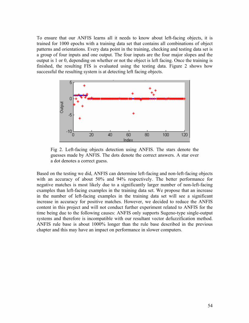
To ensure that our ANFIS learns all it needs to know about left-facing objects, it is trained for 1000 epochs with a training data set that contains all combinations of object patterns and orientations. Every data point in the training, checking and testing data set is a group of four inputs and one output. The four inputs are the four major slopes and the output is 1 or 0, depending on whether or not the object is left facing. Once the training is finished, the resulting FIS is evaluated using the testing data. Figure 2 shows how successful the resulting system is at detecting left facing objects.

Fig 2. Left-facing objects detection using ANFIS. The stars denote the guesses made by ANFIS. The dots denote the correct answers. A star over a dot denotes a correct guess.

Based on the testing we did, ANFIS can determine left-facing and non-left-facing objects with an accuracy of about 50% and 94% respectively. The better performance for negative matches is most likely due to a significantly larger number of non-left-facing examples than left-facing examples in the training data set. We propose that an increase in the number of left-facing examples in the training data set will see a significant increase in accuracy for positive matches. However, we decided to reduce the ANFIS content in this project and will not conduct further experiment related to ANFIS for the time being due to the following causes: ANFIS only supports Sugeno-type single-output systems and therefore is incompatible with our resultant vector defuzzification method. ANFIS rule base is about 1000% longer than the rule base described in the previous chapter and this may have an impact on performance in slower computers.

54

Chapter 7: Project Conclusions and Future Work 7.1 Conclusions Fuzzy Logic is currently used widely in industries all over the globe, notably in Japan. Research on fuzzy logic is often industry-driven, making a project like ours even more special. Our case studies show that fuzzy logic has been applied to motion tracking systems and strengthen our conviction that this is a feasible, albeit challenging, undertaking. Building a fuzzy logic expert system is a challenging task on multiple levels. The designer has to possess expert knowledge of the task at hand or work with someone who does. Not to mention the supporting infrastructure of this project, the worktable, the object identification system, the image acquisition and processing systems, etc, were non-existent and had to be built from scratch. Collecting data with image acquisition software for an extended period helps build our intuition as to how perfectly good data become fuzzy due to the introduction of noise in various stages of the image acquisition process. Only with this knowledge were we able to utilize fuzzy logic to solve the problem. This project is also challenging due to the great number of possible solutions to the problem—a yearlong research merely touched the tip of the iceberg. After much experimentation, we concluded that an efficient design would be to split the system into two cascaded systems: the first computes the object heading and the second, the ID. In order for the cascading inference system to work, the output of the first must be defuzzified and refuzzified into the second, and this is facilitated by the novel resultant vector defuzzification method we developed. We found that Mamdani-type fuzzy inference systems are most compatible with our methodology because it allows multiple fuzzy outputs. The fuzzy logic toolkit, as implemented in Matlab, gives the designer a myriad of membership functions to choose from. The toolkit allows us to change the inference and aggregation methods as well as customize our own methods should we find the built-in ones lacking. Due to time constraints, however, all of these options are yet unexplored. Fortunately, we found that the provided triangular-shaped and bell-shaped membership functions serve our purposes just fine. Indeed, the real task is coming up with the optimal set of parameters to use, which we accomplish through laborious analysis of hard data produced by the image processing stage. As we were exploring other ways to tune the system, we experimented with ANFIS. Our assessment of ANFIS as an optimization tool is that although it has great potential, it is incompatible with our methodology as it only generates Sugeno-type single-output inference systems. Judging from the results we obtained and outlined in the preceding chapter, we propose that fuzzy logic can be applied to position tracking and motion. The system that we built using fuzzy logic managed to guess correctly 86% of primary directions, 55% of secondary directions and 75% of tertiary directions. Although a formal statistical analysis is yet to be performed, we predict that these scores are high enough to not be the result of

55

chance and that this constitutes a trend: the more optimized the set of rules and membership functions are, the more robust the system. We believe that our success is the result of meticulous tuning and optimization that were halted as the semester draws to a close; with further work, our system will become an even more effectual fuzzy expert system. 7.2 Future Work Due to the difficulties that we faced in designing the image acquisition and processing systems, we are unable to complete the development of the fuzzy control system for motion prediction. After an object’s heading and ID have been determined, the system should compute the velocity and acceleration of an object by comparing the object’s position in several consecutive video frames. This is an important aspect to the project that is still pending. As we believe that the system can be further optimized, neuro-adaptive learning techniques is one of the things we should explore further. Perhaps there is a way to incorporate fuzzy logic into neuro-adaptive learning without being constrained to single output FIS. We should also explore other FIS designs. Perhaps the system should be broken up into three smaller systems that specialize in one direction category. Designing the rules for those systems would have been simpler. We propose that a small number of parallel neuro-adaptive systems that use the resultant-vector defuzzification outputs we came up with, would be able to significantly outperform our current FIS.

56

Bibliography 1 G Goebel, An Introduction to Fuzzy Control Systems v1.0.5, 2005 2 K B How and K B See, Motion tracking and Prediction System Utilizing Image Processing and Artificial Intelligence Technique, 2005 3 R Kay, Computerworld, Sidebar: The history of fuzzy logic, Russell Kay, 2004 4 E V Cuevas, D Zalfidar and R Rojas, Fuzzy condensed algorithm applied to control a robotic head for visual tracking, 2004 5 S H Lee, R J Howlett and S D Walters, Small Engine Control by Fuzzy Logic, 2004 6 S Syed and M E Cannon, Fuzzy Logic Based-Map Matching Algorithm for Vehicle Navigation System in Urban Canyons, 2004 7 Matlab Image Acquisition Toolbox User’s Guide Version 1, 2003 8 N Kasabov, Evolving Neuro-Fuzzy Inference Systems, 2002 9 Z H Huang and Q Shen, A New Fuzzy Interpolative Reasoning Method Based On Center of Gravity, 2002 10 M Mukaidono, Fuzzy Logic for Beginners, 2001 11 S D Kaehler, Fuzzy Logic – An Introduction, 1998 12 Matlab Fuzzy Logic Toolbox User’s Guide Version 2, 1995 13 Matlab Image Processing Toolbox User’s Guide Version 5, 1993 14 Wikipedia, www.wikipedia.org

57

58

Appendix: Code Listings %procfileimage.m %Loads an image containing objects from file and computes the direction and id of the objects function procfileimage(imFileName) %read from file image = imread(strcat(imFileName,'.jpg')); %convert to binary image image = im2bw(image); %create array A A = createa(image); %find all object centers in array A [highEnergyA, centerI, centerJ] = findcenter(A); %computes the direction and id of the object [regionMean regionCount primSec major normedPrimSec slopeRanked majorNormed degree confidence dots] = procdata(image,A,highEnergyA,centerI,centerJ); id = computeid(dots); %datalogging %print mean and count statistics printstats(regionMean,regionCount,centerI,centerJ,imFileName) %print slopes between regions printslope(primSec,major,normedPrimSec,majorNormed,slopeRanked,centerI,centerJ,imFileName) %print direction and confidence printdir(degree,confidence,centerI,centerJ,imFileName) %print id and confidence printid(dots,id,centerI,centerJ,imFileName); %debugging %imtool(strcat(imFileName, '.jpg')); %end of file

59

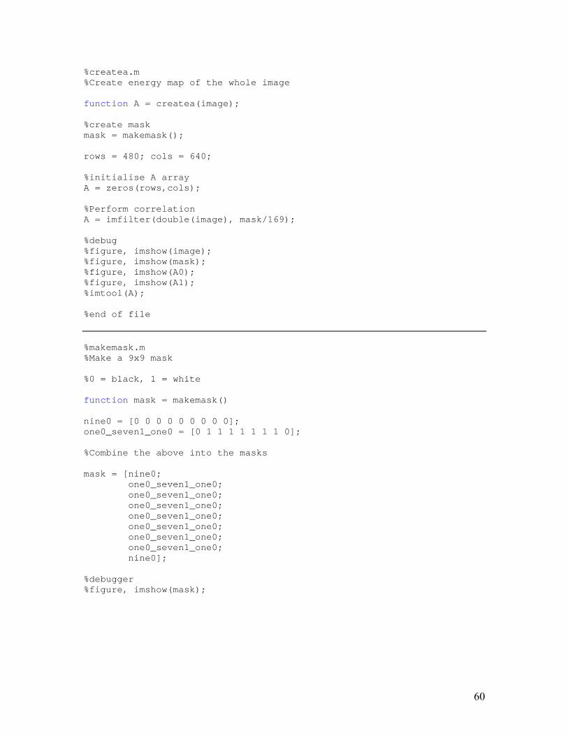
%createa.m %Create energy map of the whole image function A = createa(image); %create mask mask = makemask(); rows = 480; cols = 640; %initialise A array A = zeros(rows,cols); %Perform correlation A = imfilter(double(image), mask/169); %debug %figure, imshow(image); %figure, imshow(mask); %figure, imshow(A0); %figure, imshow(A1); %imtool(A); %end of file %makemask.m %Make a 9x9 mask %0 = black, 1 = white function mask = makemask() nine0 = [0 0 0 0 0 0 0 0 0]; one0_seven1_one0 = [0 1 1 1 1 1 1 1 0]; %Combine the above into the masks mask = [nine0; one0_seven1_one0; one0_seven1_one0; one0_seven1_one0; one0_seven1_one0; one0_seven1_one0; one0_seven1_one0; one0_seven1_one0; nine0]; %debugger %figure, imshow(mask);

60

%findcenter.m %Finding the center of objects in the energy map function [highEnergyA, centerI, centerJ] = findcenter(A) %variables %threshold = 0.78; threshold = 0.1; offset = 20;%should be equal to object's dimension offset2 = 10;%should be equal to object center rectangle dim rows = 480; cols = 640; trueObjCtr = zeros(rows,cols); centerI = 0; centerJ = 0; highEnergyA = A.*(A>threshold); objCtrA = imregionalmax(highEnergyA); [potentialI, potentialJ] = find(objCtrA); %Removing object center aliases trueObjCtr(potentialI(1), potentialJ(1)) = 1; centerI(1) = potentialI(1); centerJ(1) = potentialJ(1); for i = 2:length(potentialI), insert = 1; for j = 1:length(centerI) if(abs(potentialI(i)-centerI(j)) < offset) if(abs(potentialJ(i)-centerJ(j)) < offset) insert = 0; if(highEnergyA(potentialI(i),potentialJ(i)) >

highEnergyA(centerI(j), centerJ(j))) trueObjCtr(centerI(j), centerJ(j)) = 0; centerI(j) = potentialI(i); centerJ(j) =

potentialJ(i); trueObjCtr(potentialI(i), potentialJ(i)) = 1; break end end end end if(insert == 1) trueObjCtr(potentialI(i), potentialJ(i)) = 1; next = length(centerI)+1; centerI(next) = potentialI(i); centerJ(next) = potentialJ(i); end end %debugging purposes % imtool(A); % imtool(highEnergyA); % imtool(objCtrA); % imtool(trueObjCtr); % for i = 1:length(centerI) % figure,imshow(B(:,:,i)) % end %end of file

61

%procdata.m %Computes the direction and dots that are on in every object in the image function [regionMean regionCount primSec major normedPrimSec slopeRanked majorNormed degree confidence dots] = procdata(image,A,highEnergyA,centerI,centerJ) bdim = 21; offset = 10; B = zeros(bdim,bdim,length(centerI));% B is not a B matrix, but an array of B matrices %iterate through the clusters and record cluster data for i = 1:length(centerI) %Key %B(:,:,i) is the filtered B cluster %C(:,:,i) is the original B cluster %D(:,:,i) the original B cluster with most of center dot removed %E(:,:,i) is the filtered B cluster with center for removed %BNormed(:,:,i) is the normalized filtered B cluster centerRow = centerI(i); centerCol = centerJ(i); %shift the dots away from the edge of the image [B(:,:,i) C(:,:,i)] = correctc(A,image,centerRow,centerCol,offset); %normalization of B highestB = max(max(B(:,:,i))); BNormed(:,:) = B(:,:,i)*1/highestB; %Remove the center dot to reduce bleed over D(:,:,i) = C(:,:,i); D(8:14,8:14,i) = zeros(7); %redo FFT on D(:,:,i) mask = makemask(); E(:,:,i) = imfilter(double(D(:,:,i)), mask/169); %locate the backdot (non-fuzzy method) % [backDotEnergy backDotCol] = max(max(E(:,:,i))); % [backDotEnergy backDotRow] = max(max(E(:,:,i)')); %Statistical analysis of the cluster [regionMean(:,i) regionCount(:,i) regionMax] = computestats(E(:,:,i)); [regionMax2 regionBIndex] = max(regionMax); %compute various slopes [primSec(:,i) major(:,i) normedPrimSec(:,i) slopeRanked(:,i) majorNormed(:,i)] = computeslopes(regionMean(:,i)); %Start using fuzzy logic

62

%***************************Old Versions****************************** %DIRECTION FIS V2 %degree2 = evalfis([slopeRanked(1) slopeRanked(2) slopeRanked(3) %slopeRanked(4) slopeRanked(5) slopeRanked(6) slopeRanked(7) slopeRanked(8)], readfis('direction1')); %DIRECION FIS V3 %degree2 = evalfis([majorNormed(1) majorNormed(2) majorNormed(3) majorNormed(4)], readfis('direction1')); %degree = evalfis([degree2(1) degree2(2) degree2(3) degree2(4)degree2(5) degree2(6) degree2(7) degree2(8)], readfis('direction2')); %************************End of Old Versions************************** %************************DIRECTION FIS V4***************************** degree2 = evalfis([majorNormed(1,i) majorNormed(2,i) majorNormed(3,i) majorNormed(4,i)], readfis('direction1')); [degree(i) confidence(i)] = computedirvec(degree2); rotatedImage = imrotate(B(:,:,i),degree(i),'nearest','crop'); [regionMean2 regionCount2] = computenineregion2(rotatedImage); idSlopeNormed = computestats2(regionMean2); dots(:,i) = evalfis([idSlopeNormed(5) idSlopeNormed(8) idSlopeNormed(3) idSlopeNormed(6) idSlopeNormed(1)], readfis('id')); %************************End of FIS V4******************************** %debug % imtool(B(:,:,i)); % imtool(BNormed(:,:,i)); % imtool(C(:,:,i)); % imtool(D(:,:,i)); % imtool(E(:,:,i)); % imwrite(B(:,:,i),strcat('B_',int2str(i),'.jpg')); % imwrite(C(:,:,i),strcat('C_',int2str(i),'.jpg')); %ANFIS %datalog(i,:) = [majorNormed(1,i) majorNormed(2,i) majorNormed(3,i) majorNormed(4,i) 1]; %datalog2(i,:) = [majorNormed(1,i) majorNormed(2,i) majorNormed(3,i) majorNormed(4,i) 0]; end %data logging for ANFIS %save SouthEast_CH.dat datalog; %save SouthEast_CH2.dat datalog2; %end of file

63

%computestats.m %Takes an energy map of an object, divides it into nine regions and returns the %mean and other statistics. function [regionMean regionCount regionMax] = computestats(image1) %divide image1 into regions region(:,:,1) = image1(1:7, 1:7); region(:,:,2) = image1(1:7, 8:14); region(:,:,3) = image1(1:7, 15:21); region(:,:,4) = image1(8:14, 1:7); region(:,:,5) = image1(8:14, 8:14); region(:,:,6) = image1(8:14, 15:21); region(:,:,7) = image1(15:21, 1:7); region(:,:,8) = image1(15:21, 8:14); region(:,:,9) = image1(15:21, 15:21); %Compute the number of pixels in a region regionSize = length(region(:,:,1)).^2; %works only for a square region %Get the mean, count and max for each region %There are nine regions for i = 1:9 regionMean(i) = mean(mean(region(:,:,i))); regionCount(i) = length(find(region(:,:,i)>0))/regionSize; regionMax(i) = max(max(region(:,:,i))); end %ignore the max of the center region regionMax(5) = 0; %end of file %computeslopes.m %Computes the major and other slopes function [primSec, major, normedPrimSec, slopeRanked, majorNormed] = computeslopes(regionMean) %compute slopes primSec(1) = regionMean(5)-regionMean(1); primSec(2) = regionMean(5)-regionMean(2); primSec(3) = regionMean(5)-regionMean(3); primSec(4) = regionMean(5)-regionMean(4); primSec(5) = regionMean(5)-regionMean(6); primSec(6) = regionMean(5)-regionMean(7); primSec(7) = regionMean(5)-regionMean(8); primSec(8) = regionMean(5)-regionMean(9); major(1) = regionMean(4)-regionMean(6); major(2) = regionMean(2)-regionMean(8); major(3) = regionMean(1)-regionMean(9); major(4) = regionMean(3)-regionMean(7); %normalize primary and secondary slopes normalizer = abs(primSec(1));

64

for i = 2:8 if(abs(primSec(i)) > normalizer) normalizer = abs(primSec(i)); end end %just in case it's a null pic check if normalizer is 0 %if so set it to 1; if(normalizer == 0) normalizer = 1; end for i = 1:8 normedPrimSec(i) = primSec(i)/normalizer; end %compute unsigned major slope for i = 1:4 majorUnsig(i) = abs(major(i)); end %normalize major slopes normalizer = majorUnsig(1); for i = 2:4 if(majorUnsig(i) > normalizer) normalizer = majorUnsig(i); end end %just in case it's a null pic check if normalizer is 0 %if so set it to 1; if(normalizer == 0) normalizer = 1; end for i = 1:4 majorNormed(i) = najor(i)/normalizer; end %initialize slopeRanked slopeRanked = zeros(length(normedPrimSec),1); %rank the slopes from smallest to largest %note: the smallest slope should be the center-backdot slope slope_sorted = sort(normedPrimSec); for i = 1:length(slope_sorted) for j = 1:length(normedPrimSec) if(normedPrimSec(j) == slope_sorted(i) && slopeRanked(j) == 0) slopeRanked(j) = i; end end end %end of file

65

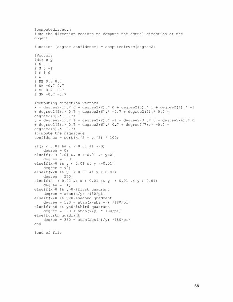
%computedirvec.m %Use the direction vectors to compute the actual direction of the object function [degree confidence] = computedirvec(degree2) %Vectors %dir x y % N 0 1 % S 0 -1 % E 1 0 % W -1 0 % NE 0.7 0.7 % NW -0.7 0.7 % SE 0.7 -0.7 % SW -0.7 -0.7 %computing direction vectors x = degree2(1).* 0 + degree2(2).* 0 + degree2(3).* 1 + degree2(4).* -1 + degree2(5).* 0.7 + degree2(6).* -0.7 + degree2(7).* 0.7 + degree2(8).* -0.7; y = degree2(1).* 1 + degree2(2).* -1 + degree2(3).* 0 + degree2(4).* 0 + degree2(5).* 0.7 + degree2(6).* 0.7 + degree2(7).* -0.7 + degree2(8).* -0.7; %compute the magnitude confidence = sqrt(x.^2 + y.^2) * 100; if(x < 0.01 && x >-0.01 && y>0) degree = 0; elseif(x < 0.01 && x >-0.01 && y<0) degree = 180; elseif(x>0 && y < 0.01 && y >-0.01) degree = 90; elseif(x<0 && y < 0.01 && y >-0.01) degree = 270; elseif(x < 0.01 && x >-0.01 && y < 0.01 && y >-0.01) degree = -1; elseif(x>0 && y>0)%first quadrant degree = atan(x/y) *180/pi; elseif(x>0 && y<0)%second quadrant degree = 180 - atan(x/abs(y)) *180/pi; elseif(x<0 && y<0)%third quadrant degree = 180 + atan(x/y) * 180/pi; else%fourth quadrant degree = 360 - atan(abs(x)/y) *180/pi; end %end of file

66

%computenineregion2.m %Takes an energy map and returns 9 regions function [regionMean regionCount] = computenineregion2(B) region(:,:,1) = B(1:7, 1:7); region(:,:,2) = B(1:7, 8:14); region(:,:,3) = B(1:7, 15:21); region(:,:,4) = B(8:14, 1:7); region(:,:,5) = B(8:14, 8:14); region(:,:,6) = B(8:14, 15:21); region(:,:,7) = B(15:21, 1:7); region(:,:,8) = B(15:21, 8:14); region(:,:,9) = B(15:21, 15:21); regionSize = length(region(:,:,1)).^2; for i = 1:9 regionMean(i) = mean(mean(region(:,:,i))); regionCount(i) = length(find(region(:,:,i)>0))/regionSize; end %end of file %computestats2.m %Compute the normalized slopes function slopeNormed = computestats2(regionMean) %compute slopes primSec(1) = regionMean(5)-regionMean(1); primSec(2) = regionMean(5)-regionMean(2); primSec(3) = regionMean(5)-regionMean(3); primSec(4) = regionMean(5)-regionMean(4); primSec(5) = regionMean(5)-regionMean(6); primSec(6) = regionMean(5)-regionMean(7); primSec(7) = regionMean(5)-regionMean(8); primSec(8) = regionMean(5)-regionMean(9); %normalize primary and secondary slopes normalizer = primSec(1); for i = 2:8 if(primSec(i) > normalizer) normalizer = primSec(i); end end for i = 1:8 slopeNormed(i) = primSec(i)/normalizer; end %end of file

67

%printstats.m %print the stats of the nine regions of the energy map function printstats(regionMean,regionCount,centerI,centerJ,imFileName) fid = fopen(strcat('sts_', imFileName, '.txt'),'w'); fprintf(fid,strcat('#',imFileName,'\n')); fprintf(fid, 'no. row col _UL__ _UC__ _UR__ _ML__ _MC__ _MR__ _LL__ _LC__ _LR__ _ULC_ _UCC_ _URC_ _MLC_ _MCC_ _MRC_ _LLC_ _LCC_ _LRC_\n'); for i=1:length(centerI) fprintf(fid, '%3d %3d %3d ',i,centerI(i),centerJ(i)); fprintf(fid, '%5.3f %5.3f %5.3f ',regionMean(1,i), regionMean(2,i), regionMean(3,i)); fprintf(fid, '%5.3f %5.3f %5.3f ',regionMean(4,i), regionMean(5,i), regionMean(6,i)); fprintf(fid, '%5.3f %5.3f %5.3f ',regionMean(7,i), regionMean(8,i), regionMean(9,i)); fprintf(fid, '%5.3f %5.3f %5.3f ',regionCount(1,i), regionCount(2,i), regionCount(3,i)); fprintf(fid, '%5.3f %5.3f %5.3f ',regionCount(4,i), regionCount(5,i), regionCount(6,i)); fprintf(fid, '%5.3f %5.3f %5.3f \n',regionCount(7,i), regionCount(8,i), regionCount(9,i)); end fclose(fid); %end of file %printslope.m %Print the computed slopes function printslope(primSec,major,slopeNormed,majorNormed,slopeRanked,centerI,centerJ,imFileName) fid = fopen(strcat('grad_', imFileName, '.txt'), 'w'); fprintf(fid, strcat('#',imFileName,'\n')); fprintf(fid, 'no. row col MC-UL MC-UC MC-UR MC-ML MC-MR MC-LL MC-LC MC-LR ML-MR UC-LC UL-LR UR-LL\n'); for i=1:length(centerI) %print slopes fprintf(fid, '%3d %3d %3d ',i,centerI(i),centerJ(i)); fprintf(fid, '%5.2f %5.2f ',primSec(1,i),primSec(2,i)); fprintf(fid, '%5.2f %5.2f ',primSec(3,i),primSec(4,i)); fprintf(fid, '%5.2f %5.2f ',primSec(5,i),primSec(6,i)); fprintf(fid, '%5.2f %5.2f ',primSec(7,i),primSec(8,i)); fprintf(fid, '%5.2f %5.2f ',major(1,i),major(2,i)); fprintf(fid, '%5.2f %5.2f\n',major(3,i),major(4,i)); %print normalized slopes fprintf(fid, '%3d %3d %3d ',i,centerI(i),centerJ(i));

68

fprintf(fid, '%5.2f %5.2f ',slopeNormed(1,i),slopeNormed(2,i)); fprintf(fid, '%5.2f %5.2f ',slopeNormed(3,i),slopeNormed(4,i)); fprintf(fid, '%5.2f %5.2f ',slopeNormed(5,i),slopeNormed(6,i)); fprintf(fid, '%5.2f %5.2f ',slopeNormed(7,i),slopeNormed(8,i)); fprintf(fid, '%5.2f %5.2f ',majorNormed(1,i) ,majorNormed(2,i)); fprintf(fid, '%5.2f %5.2f normalized\n',majorNormed(3,i) ,majorNormed(4,i)); %print according to rank fprintf(fid, '%3d %3d %3d ',i,centerI(i),centerJ(i)); fprintf(fid, '%5.2f %5.2f ',slopeRanked(1,i),slopeRanked(2,i)); fprintf(fid, '%5.2f %5.2f ',slopeRanked(3,i),slopeRanked(4,i)); fprintf(fid, '%5.2f %5.2f ',slopeRanked(5,i),slopeRanked(6,i)); fprintf(fid, '%5.2f %5.2f ranked\n',slopeRanked(7,i),slopeRanked(8,i)); end fclose(fid); %end of file

%printdir.m %Print the computed directions of the objects function printdir(degree, confidence, centerI, centerJ, imFileName) fid = fopen(strcat('dir_', imFileName, '.txt'), 'w'); fprintf(fid, strcat('#',imFileName,'\n')); fprintf(fid, 'no. row col dir con\n'); for i = 1:size(degree,2) fprintf(fid, '%3d %3d %3d %3d %3d \n', i, centerI(i), centerJ(i), cast(degree(i),'uint32'), cast(confidence(i),'uint32')); end fclose(fid); %end of file

%printid.m %Print the computed IDs of the objects function printid(dots,id,centerI,centerJ,imFileName) fid = fopen(strcat('id_', imFileName, '.txt'), 'w'); fprintf(fid, strcat('#',imFileName,'\n')); fprintf(fid, 'no. row col _con_ LRDot URDot LLDot ULDot id\n'); for i=1:length(centerI) fprintf(fid, '%3d %3d %3d ',i,centerI(i),centerJ(i)); fprintf(fid, '%5.3f %5.3f %5.3f %5.3f %5.3f %2d \n',dots(1,i), dots(2,i), dots(3,i), dots(4,i) , dots(5,i), id(i)); end fclose(fid); %end of file

69

%procnewimage.m %Similar to procfileimage.m but obtains the image from camera instead of %reading from file function procnewimage(imFileName) %camera initialization vid = camsetup(); aMean = 0; while(aMean == 0) image = grabframe(vid); aMean = mean(mean(image)); end imwrite(image, strcat(imFileName,'.jpg')); A = createa(image); [highEnergyA, centerI, centerJ] = findcenter(A); [regionMean regionCount primSec major normedPrimSec slopeRanked majorNormed degree confidence dots] = procdata(imFileName,image,A,highEnergyA,centerI,centerJ); %datalogging %print mean and count statistics printstats(regionMean,regionCount,centerI,centerJ,imFileName) %print slopes between regions printslope(primSec,major,slopeNormed,majorNormed,slopeRanked,centerI,centerJ,imFileName) %print direction and confidence printdir(degree,confidence,centerI,centerJ,imFileName) %print id and confidence printid(dots,centerI,centerJ,imFileName); %debugging %imtool(strcat(imFileName, '.jpg')); %end of file

70

%camsetup.m %Define camera settings function vid = camsetup() vid = videoinput('winvideo',1,'RGB24_640x480'); src = getselectedsource(vid); set(src, 'ExposureMode', 'manual'); set(src, 'Exposure', 72); set(src, 'Brightness', 48); set(src, 'Contrast', 20); set(src, 'Sharpness', 73); set(src, 'Gamma', 58); %end of file

%grabframe.m %Captures a snapshot of the worktable function bw_image = grabframe(vid) %image grabbing start(vid); data = getdata(vid,5); stop(vid); image = data(:,:,:,5); %image processing northcut = 30; southcut = 30; eastcut = 30; westcut = 30; bw_image = zeros(480,640); image = image(eastcut:480-westcut, northcut:640-southcut); bw_image(eastcut:480-westcut, northcut:640-southcut) = im2bw(image,0.4); %end of file %takepic.m %Take a picture of the worktable and saves it function takepic(imFileName) %camera initialization vid = camsetup(); aMean = 0; while(aMean == 0) image = grabframe(vid); aMean = mean(mean(image)); end imwrite(image, strcat(imFileName,'.jpg')); %end of file

71

%testsuite.m %Evaluates the accuracy of the direction and ID FIS function testsuite load TSImagesB load TSKeyB %Guide: %key(a,b,c) %a = object index (1-16 since 0 is included). %b = 1 is degree, b = 2 is id. %c = image index (1-32). %result(d,e,f) %d = object index (1-16 since 0 is included). %e = 1 is degree, b = 2 is id. %f = image index (1-32). %COMPUTE RESULTS for i = 1:32 % if(i==19) %debug mode [result(:,1,i) result(:,2,i)] = procimage(testImage(:,:,i)); % end end %COMPUTE ACCURACY tolerance = 25; %plus minus tolerance primaryCnt = 0; %iterate through the images for i = 1:32 % if(i == 19) degCorrect = 0; idCorrect = 0; %iterate through the objects in an image for j = 1:16 if(result(j,1,i) >= key(j,1,i)-tolerance && result(j,1,i)

<= key(j,1,i)+tolerance) degCorrect = degCorrect + 1; end if(result(j,2,i) == key(j,2,i)) idCorrect = idCorrect + 1; end end accuracy(1,i) = degCorrect/16*100; accuracy(2,i) = idCorrect/16*100; % end end fid = fopen('V41.txt','w'); fprintf(fid, 'no dir id \n');

72

primDirAcc = 0; primIdAcc = 0; secDirAcc = 0; secIdAcc = 0; terDirAcc = 0; terIdAcc = 0; for i=1:32 fprintf(fid, '%2d %3.0f %2.0f \n',i,accuracy(1,i),accuracy(2,i)); %compute summary if(i==1 || i==2 || i==3 || i==4 || i==9 || i==10 || i==11 || i==12) primDirAcc = primDirAcc + accuracy(1,i); primIdAcc = primIdAcc + accuracy(2,i); elseif(i==5 || i==6 || i==7 || i==8 || i==13 || i==14 || i==15 || i==16) secDirAcc = secDirAcc + accuracy(1,i); secIdAcc = secIdAcc + accuracy(2,i); else terDirAcc = terDirAcc + accuracy(1,i); terIdAcc = terIdAcc + accuracy(2,i); end end fprintf(fid, 'Summary\n'); fprintf(fid, 'Primary Direction: %2.0f\n', primDirAcc/8); fprintf(fid, 'Primary ID: %2.0f\n', primIdAcc/8); fprintf(fid, 'Secondary Direction: %2.0f\n', secDirAcc/8); fprintf(fid, 'Secondary ID: %2.0f\n', secIdAcc/8); fprintf(fid, 'Tertiary Direction: %2.0f\n', terDirAcc/16); fprintf(fid, 'Tertiary Direction: %2.0f\n', terIdAcc/16); fclose(fid); %end of file

73